Embed Size (px)
Citation preview
ENG1091
Mathematics for Engineering
Lecture notes
Clayton Campus2014 Campus
Australia Malaysia South Africa Italy India monash.edu/science

School of Mathematical Sciences Monash University
Contents
1. Vectors in 3-dimensions 3
1.1 Introduction . . . . . . . . . . . . . . . . . . . . . . . . . . . . . . . . . . . 4
1.1.1 Notation . . . . . . . . . . . . . . . . . . . . . . . . . . . . . . . . . 4
1.1.2 Algebraic properties . . . . . . . . . . . . . . . . . . . . . . . . . . 4
1.2 Vector Dot Product . . . . . . . . . . . . . . . . . . . . . . . . . . . . . . . 5
1.2.1 Unit Vectors . . . . . . . . . . . . . . . . . . . . . . . . . . . . . . . 6
1.3 Vector Cross Product . . . . . . . . . . . . . . . . . . . . . . . . . . . . . . 7
1.3.1 Interpreting the cross product . . . . . . . . . . . . . . . . . . . . . 7
1.3.2 Right Hand Thumb rule . . . . . . . . . . . . . . . . . . . . . . . . 8
1.4 Scalar and Vector projections . . . . . . . . . . . . . . . . . . . . . . . . . 9
1.4.1 Scalar Projections . . . . . . . . . . . . . . . . . . . . . . . . . . . . 9
1.4.2 Vector Projection . . . . . . . . . . . . . . . . . . . . . . . . . . . . 9
2. Three-Dimensional Euclidean Geometry. Lines. 11
2.1 Lines in 3-dimensional space . . . . . . . . . . . . . . . . . . . . . . . . . . 12
2.2 Vector equation of a line . . . . . . . . . . . . . . . . . . . . . . . . . . . . 13
3. Three-Dimensional Euclidean Geometry. Planes. 14
3.1 Planes in 3-dimensional space . . . . . . . . . . . . . . . . . . . . . . . . . 15
3.1.1 Constructing the equation of a plane . . . . . . . . . . . . . . . . . 15
3.1.2 Parametric equations for a plane . . . . . . . . . . . . . . . . . . . 16
3.2 Vector equation of a plane . . . . . . . . . . . . . . . . . . . . . . . . . . . 17
4. Linear systems of equations 19
4.1 Examples of Linear Systems . . . . . . . . . . . . . . . . . . . . . . . . . . 20
4.1.1 Bags of coins . . . . . . . . . . . . . . . . . . . . . . . . . . . . . . 20
4.1.2 Silly puzzles . . . . . . . . . . . . . . . . . . . . . . . . . . . . . . . 20
4.1.3 Intersections of planes . . . . . . . . . . . . . . . . . . . . . . . . . 20
4.2 A standard strategy . . . . . . . . . . . . . . . . . . . . . . . . . . . . . . 21
4.3 Lines and planes . . . . . . . . . . . . . . . . . . . . . . . . . . . . . . . . 22
5. Gaussian Elimination 25
5.1 Gaussian elimination and back-substitution . . . . . . . . . . . . . . . . . 26
5.2 Gaussian elimination . . . . . . . . . . . . . . . . . . . . . . . . . . . . . . 26
26-Jul-2014 2
School of Mathematical Sciences Monash University
5.2.1 Gaussian elimination strategy . . . . . . . . . . . . . . . . . . . . . 27
5.3 Exceptions . . . . . . . . . . . . . . . . . . . . . . . . . . . . . . . . . . . . 27
6. Matrices 29
6.1 Matrices . . . . . . . . . . . . . . . . . . . . . . . . . . . . . . . . . . . . . 30
6.1.1 Notation . . . . . . . . . . . . . . . . . . . . . . . . . . . . . . . . . 31
6.1.2 Operations on matrices . . . . . . . . . . . . . . . . . . . . . . . . . 31
6.1.3 Some special matrices . . . . . . . . . . . . . . . . . . . . . . . . . 32
6.1.4 Properties of matrices . . . . . . . . . . . . . . . . . . . . . . . . . 32
6.1.5 Notation . . . . . . . . . . . . . . . . . . . . . . . . . . . . . . . . . 33
7. Inverses of Square Matrices. 34
7.1 Matrix Inverse . . . . . . . . . . . . . . . . . . . . . . . . . . . . . . . . . 35
7.1.1 Inverse by Gaussian elimination . . . . . . . . . . . . . . . . . . . . 35
7.2 Determinants . . . . . . . . . . . . . . . . . . . . . . . . . . . . . . . . . . 36
7.2.1 Notation . . . . . . . . . . . . . . . . . . . . . . . . . . . . . . . . . 36
7.3 Inverse using determinants . . . . . . . . . . . . . . . . . . . . . . . . . . . 37
7.4 Vector Cross Products . . . . . . . . . . . . . . . . . . . . . . . . . . . . . 38
8. Eigenvalues and eigenvectors. 39
8.1 Introduction . . . . . . . . . . . . . . . . . . . . . . . . . . . . . . . . . . . 40
8.2 Eigenvalues . . . . . . . . . . . . . . . . . . . . . . . . . . . . . . . . . . . 41
8.3 Decomposing Symmetric matrices . . . . . . . . . . . . . . . . . . . . . . . 44
8.4 Matrix inverse . . . . . . . . . . . . . . . . . . . . . . . . . . . . . . . . . . 46
8.5 The Cayley-Hamilton theorem: Not examinable . . . . . . . . . . . . . . . 47
9. Hyperbolic functions 49
9.1 Hyperbolic functions . . . . . . . . . . . . . . . . . . . . . . . . . . . . . . 50
9.1.1 Hyperbolic functions . . . . . . . . . . . . . . . . . . . . . . . . . . 51
9.1.2 More hyperbolic functions . . . . . . . . . . . . . . . . . . . . . . . 52
9.2 Special functions: not examinable . . . . . . . . . . . . . . . . . . . . . . . 53
10. Integration 55
10.1 Integration : Revision . . . . . . . . . . . . . . . . . . . . . . . . . . . . . 56
10.1.1 Some basic integrals . . . . . . . . . . . . . . . . . . . . . . . . . . 57
10.1.2 Substitution . . . . . . . . . . . . . . . . . . . . . . . . . . . . . . 57
26-Jul-2014 3
School of Mathematical Sciences Monash University
10.2 Integration by parts . . . . . . . . . . . . . . . . . . . . . . . . . . . . . . 57
11. Improper integrals 60
11.1 Improper Integrals . . . . . . . . . . . . . . . . . . . . . . . . . . . . . . . 61
11.1.1 A standard strategy . . . . . . . . . . . . . . . . . . . . . . . . . . 61
12. Comparison test for convergence 65
12.1 Comparison Test for Improper Integrals . . . . . . . . . . . . . . . . . . . 66
12.2 The General Strategy . . . . . . . . . . . . . . . . . . . . . . . . . . . . . 68
13. Introduction to sequences and series. 70
13.1 Definitions . . . . . . . . . . . . . . . . . . . . . . . . . . . . . . . . . . . 71
13.1.1 Notation . . . . . . . . . . . . . . . . . . . . . . . . . . . . . . . . 71
13.1.2 Partial sums . . . . . . . . . . . . . . . . . . . . . . . . . . . . . . 71
13.1.3 Arithmetic series . . . . . . . . . . . . . . . . . . . . . . . . . . . . 72
13.1.4 Fibonacci sequence . . . . . . . . . . . . . . . . . . . . . . . . . . 72
13.1.5 Geometric series . . . . . . . . . . . . . . . . . . . . . . . . . . . . 73
13.1.6 Compound Interest . . . . . . . . . . . . . . . . . . . . . . . . . . 73
14. Convergence of series. 75
14.1 Infinite series . . . . . . . . . . . . . . . . . . . . . . . . . . . . . . . . . . 76
14.1.1 Convergence and divergence . . . . . . . . . . . . . . . . . . . . . 76
14.2 Tests for convergence . . . . . . . . . . . . . . . . . . . . . . . . . . . . . 76
14.2.1 Zero tail? . . . . . . . . . . . . . . . . . . . . . . . . . . . . . . . . 76
14.2.2 The Comparison test . . . . . . . . . . . . . . . . . . . . . . . . . 76
15. Integral and ratio tests. 78
15.1 The Integral Test . . . . . . . . . . . . . . . . . . . . . . . . . . . . . . . 80
15.2 The Ratio test . . . . . . . . . . . . . . . . . . . . . . . . . . . . . . . . . 81
16. Comparison test, alternating series. 83
16.1 Alternating series . . . . . . . . . . . . . . . . . . . . . . . . . . . . . . . 84
16.2 Non-positive infinite series . . . . . . . . . . . . . . . . . . . . . . . . . . 85
16.3 Re-ordering an infinite series . . . . . . . . . . . . . . . . . . . . . . . . . 85
17. Power series 87
17.1 Simple power series . . . . . . . . . . . . . . . . . . . . . . . . . . . . . . 88
26-Jul-2014 4

School of Mathematical Sciences Monash University
17.2 The general power series . . . . . . . . . . . . . . . . . . . . . . . . . . . 88
17.3 Examples of Power Series . . . . . . . . . . . . . . . . . . . . . . . . . . . 89
17.4 Maclaurin Series . . . . . . . . . . . . . . . . . . . . . . . . . . . . . . . . 89
17.5 Taylor Series . . . . . . . . . . . . . . . . . . . . . . . . . . . . . . . . . . 90
17.6 Uniqueness . . . . . . . . . . . . . . . . . . . . . . . . . . . . . . . . . . . 91
18. Radius of convergence 93
18.1 Radius of convergence . . . . . . . . . . . . . . . . . . . . . . . . . . . . . 94
18.2 Computing the Radius of Convergence . . . . . . . . . . . . . . . . . . . 94
18.3 Some theorems . . . . . . . . . . . . . . . . . . . . . . . . . . . . . . . . . 95
19. Function Approximation using Taylor Series 96
19.1 Motivation . . . . . . . . . . . . . . . . . . . . . . . . . . . . . . . . . . . 97
19.2 Taylor polynomials . . . . . . . . . . . . . . . . . . . . . . . . . . . . . . 97
19.3 Accuracy . . . . . . . . . . . . . . . . . . . . . . . . . . . . . . . . . . . . 100
19.4 Using Taylor series to calculate limits . . . . . . . . . . . . . . . . . . . . 102
19.5 l’Hopital’s rule. . . . . . . . . . . . . . . . . . . . . . . . . . . . . . . . . 103
20. Remainder term for Taylor series. 106
20.1 Motivation . . . . . . . . . . . . . . . . . . . . . . . . . . . . . . . . . . . 107
20.2 Integration by parts and Taylor series . . . . . . . . . . . . . . . . . . . . 107
21. Introduction to ODEs 111
21.1 Motivation . . . . . . . . . . . . . . . . . . . . . . . . . . . . . . . . . . . 112
21.2 Definitions . . . . . . . . . . . . . . . . . . . . . . . . . . . . . . . . . . . 112
21.3 Solution strategies . . . . . . . . . . . . . . . . . . . . . . . . . . . . . . . 113
21.4 General and particular solutions . . . . . . . . . . . . . . . . . . . . . . . 115
22. Separable first order ODEs. 116
22.1 Separable equations . . . . . . . . . . . . . . . . . . . . . . . . . . . . . . 117
22.2 First order linear ODEs . . . . . . . . . . . . . . . . . . . . . . . . . . . . 118
22.2.1 Solving the homogeneous ODE . . . . . . . . . . . . . . . . . . . . 120
22.2.2 Finding a particular solution . . . . . . . . . . . . . . . . . . . . . 121
23. The integrating factor. 122
23.1 The Integrating Factor . . . . . . . . . . . . . . . . . . . . . . . . . . . . 123
26-Jul-2014 5

School of Mathematical Sciences Monash University
24. Homogeneous Second order ODEs. 125
24.1 Second order linear ODEs . . . . . . . . . . . . . . . . . . . . . . . . . . 126
24.2 Homogeneous equations . . . . . . . . . . . . . . . . . . . . . . . . . . . . 126
25. Non-Homogeneous Second order ODEs. 131
25.1 Non-homogeneous equations . . . . . . . . . . . . . . . . . . . . . . . . . 132
25.2 Undetermined coefficients . . . . . . . . . . . . . . . . . . . . . . . . . . . 133
25.3 Exceptions . . . . . . . . . . . . . . . . . . . . . . . . . . . . . . . . . . . 134
26. Coupled systems of ODEs 135
26.1 Motivation . . . . . . . . . . . . . . . . . . . . . . . . . . . . . . . . . . . 136
26.2 First method: differentiation . . . . . . . . . . . . . . . . . . . . . . . . . 136
26.3 Second method: eigenvectors and eigenvalues . . . . . . . . . . . . . . . . 138
27. Applications of Differential Equations 141
27.1 Applications of ODEs . . . . . . . . . . . . . . . . . . . . . . . . . . . . . 142
27.2 Newton’s law of cooling . . . . . . . . . . . . . . . . . . . . . . . . . . . . 142
27.3 Pollution in swimming pools . . . . . . . . . . . . . . . . . . . . . . . . . 143
27.4 Newtonian mechanics . . . . . . . . . . . . . . . . . . . . . . . . . . . . . 144
28. Functions of Several Variables 147
28.1 Introduction . . . . . . . . . . . . . . . . . . . . . . . . . . . . . . . . . . 148
28.2 Definition . . . . . . . . . . . . . . . . . . . . . . . . . . . . . . . . . . . 148
28.3 Notation . . . . . . . . . . . . . . . . . . . . . . . . . . . . . . . . . . . . 148
28.4 Surfaces . . . . . . . . . . . . . . . . . . . . . . . . . . . . . . . . . . . . 149
28.5 Alternative forms . . . . . . . . . . . . . . . . . . . . . . . . . . . . . . . 152
29. Partial derivatives 154
29.1 First derivatives . . . . . . . . . . . . . . . . . . . . . . . . . . . . . . . . 155
29.2 Higher derivatives . . . . . . . . . . . . . . . . . . . . . . . . . . . . . . . 156
29.3 Notation . . . . . . . . . . . . . . . . . . . . . . . . . . . . . . . . . . . . 157
29.4 Exceptions : when derivatives do not exist . . . . . . . . . . . . . . . . . 158
30. Chain Rule, Gradient and Directional derivatives 160
30.1 The Chain Rule . . . . . . . . . . . . . . . . . . . . . . . . . . . . . . . . 161
30.2 Gradient and Directional Derivative . . . . . . . . . . . . . . . . . . . . . 163
26-Jul-2014 6

School of Mathematical Sciences Monash University
31. Tangent planes and linear approximations 166
31.1 Tangent planes . . . . . . . . . . . . . . . . . . . . . . . . . . . . . . . . . 167
31.2 Linear Approximations . . . . . . . . . . . . . . . . . . . . . . . . . . . . 168
32. Maxima and minima 170
32.1 Maxima and minima . . . . . . . . . . . . . . . . . . . . . . . . . . . . . 171
32.2 Local extrema . . . . . . . . . . . . . . . . . . . . . . . . . . . . . . . . . 172
32.3 Notation . . . . . . . . . . . . . . . . . . . . . . . . . . . . . . . . . . . . 173
32.4 Maxima, Minima or Saddle point? . . . . . . . . . . . . . . . . . . . . . . 173
26-Jul-2014 7
SCHOOL OF MATHEMATICAL SCIENCES
ENG1091
Mathematics for Engineering
1. Vectors in 3-dimensions

School of Mathematical Sciences Monash University
1.1 Introduction
These can be defined in (at least) two ways, algebraically as objects like
v˜
= (1, 7, 3)
u˜
= (2,−1, 4)
or geometrically as arrows in space.
How can we be sure that these two definitions actually describe the same object? Equally,how do we convert from one form to the other? That is, given (1, 2, 7) how do we drawthe arrow and likewise, given the arrow how do we extract the numbers (1, 2, 7)?
Suppose we are give two points P and Q. Suppose also that we find the change incoordinates from P to Q is (say) (1, 2, 7). We could also draw an arrow from P to Q.Thus we have two ways of recording the path from P to Q, either as the numbers (1, 2, 7)or the arrow.
Suppose now that we have another pair of points R and S and further that we find thechange in coordinates to be (1, 2, 7). Again, we can join the points with an arrow. Thisarrow will have the same direction and length as that for P to Q.
In both cases, the displacement, from start to finish, is represented by either the numbers(1, 2, 7) or the arrow – thus we can use either form to represent the vector. Note that thismeans that a vector does not live at any one place in space – it can be moved anywhereprovided its length and direction are unchanged.
To extract the numbers (1, 2, 7) given just the arrow simply place the arrow somewherein the x, y, z space, and the measure the change in coordinates from tail to tip of thevector. Equally, to draw the vector given the numbers (1, 2, 7) is easy – choose (0, 0, 0)as the tail then the point (1, 2, 7) is the tip.
1.1.1 Notation
The components of a vector are just the numbers we use to describe the vector. In theabove, the components of v
˜are 1,2 and 7.
Another very very common way to write a vector, such as v˜
= (1, 7, 3) for example, isv˜
= 1 i˜
+ 7j
˜+ 3k
˜. The three vectors i
˜, j
˜, k˜
are a simple way to remind us that thethree numbers in v
˜= (1, 7, 3) refer to directions parallel to the three coordinate axes
(with i˜
parallel to the x-axis, j
˜parallel to the y-axis and k
˜parallel to the z-axis).
In this way we can always write down any 3-dimensional vector as a linear combinationof the i
˜, j
˜, k˜
and thus these vectors are also known as basis vectors.
1.1.2 Algebraic properties
What rules must we observe in playing with vectors?
26-Jul-2014 9

School of Mathematical Sciences Monash University
I Equalityv˜
= w˜
only when the arrows for v˜
and w˜
are identical.
I StretchingThe vector λv
˜is parallel to v
˜but is stretched by a factor λ.
I AdditionTo add two vectors v
˜and w
˜arrange the two so that they are tip to tail. Then
v˜
+ w˜
is the vector that starts at the first tail and ends at the second tip.
Example 1.1
Express each of the above rules in terms of the components of vectors (i.e. in terms ofnumbers like (1, 2, 7) and (a, b, c)).
Example 1.2
Given v˜
= (3, 4, 2) and w˜
= (1, 2, 3) compute v˜
+ w˜
and 2v˜
+ 7w˜
.
Example 1.3
Given v˜
= (1, 2, 7) draw v˜
, 2v˜
and −v˜
.
Example 1.4
Given v˜
= (1, 2, 7) and w˜
= (3, 4, 5) draw and compute v˜− w˜
.
1.2 Vector Dot Product
How do we multiply vectors? We have already seen one form, stretching, v˜→ λv
˜. This
is called scalar multiplication.
Here is another form. Let v˜
= (vx, vy, vz) and w˜
= (wx, wy, wz) be a pair of vectors thenwe define the dot product v
˜· w˜
by
v˜· w˜
= vxwx + vywy + vzwz
Example 1.5
Let v˜
= (1, 2, 7) and w˜
= (−1, 3, 4). Compute v˜· v˜
, w˜· w˜
and v˜· w˜
What do we observe?
I v˜· w˜
is a single number not a vector
I v˜· w˜
= w˜· v˜
I (λv˜
) · w˜
= λ(v˜· w˜
)
I (a˜
+ b˜
) · v˜
= a˜· v˜
+ b˜· v˜
The last two cases display what we call linearity.
26-Jul-2014 10

School of Mathematical Sciences Monash University
Example 1.6 : Length of a vector
Let v˜
= (1, 2, 7). Compute the distance from (0, 0, 0) to (1, 2, 7). Compare this with√v˜· v˜
.
We can now show thatv˜· w˜
= |v||w| cos θ
where
|v| = the length of v˜
=(v2x + v2
y + v2z
)1/2
|w| = the length of w˜
=(w2x + w2
y + w2z
)1/2
and θ is the angle between the two vectors.
How do we prove this? Simple start with v˜− w˜
and compute its length,
|v − w|2 = (v˜− w˜
) · (v˜− w˜
)
= v˜· v˜− v˜· w˜− w˜· v˜
+ w˜· w˜
= |v|2 + |w|2 − 2v˜· w˜
and from the Cosine Rule for triangles we know
|v − w|2 = |v|2 + |w|2 − 2|v||w| cos θ
Thus we havev˜· w˜
= |v||w| cos θ
This gives us a convenient way to compute the angle between any pair of vectors. Ifwe find cos θ = 0 then we say that v
˜and w
˜are orthogonal (sometimes also called
perpendicular).
Thus v˜
and w˜
are orthogonal when v˜· w˜
= 0 (provided neither v˜
nor w˜
are zero).
Example 1.7
Find the angle between the vectors v˜
= (2, 7, 1) and w˜
= (3, 4,−2)
1.2.1 Unit Vectors
A vector is said to be a unit vector if its length is one. That is, v˜
is a unit vector whenv˜· v˜
= 1.
26-Jul-2014 11

School of Mathematical Sciences Monash University
1.3 Vector Cross Product
This is another way to multiply vectors. Start with v˜
= (vx, vy, vz) and w˜
= (wx, wy, wz).Then we define the cross product v
˜× w˜
by
v˜× w˜
= (vywz − vzwy, vzwx − vxwz, vxwy − vywx)
From this definition we observe
I v˜× w˜
is a vector
I v˜× w˜
= −w˜× v˜
I v˜× v˜
= 0˜
I (λv˜
)× w˜
= λ(v˜× w˜
)
I (a˜
+ b˜
)× v˜
= a˜× v˜
+ b˜× v˜
I (v˜× w˜
) · v˜
= (v˜× w˜
) · w˜
= 0˜
Example 1.8
Verify all of the above.
Example 1.9
Given v˜
= (1, 2, 7) and w˜
= (−2, 3, 5) compute v˜×w˜
, and its dot product with each ofv˜
and w˜
.
1.3.1 Interpreting the cross product
We know that v˜× w˜
is a vector and we know how to compute it. But can we describethis vector? First we need a vector, so let’s assume that v
˜×w˜6= 0˜
. Then what can wesay about the direction and length of v
˜× w˜
?
The first thing we should note is that the cross product is a vector which is orthogonalto both of the original vectors. Thus v
˜× w˜
is a vector that is orthogonal to v˜
and tow˜
. This fact follows from the definition of the cross product.
Thus we must havev˜× w˜
= λn˜
where n˜
is a unit vector orthogonal to both v˜
and w˜
and λ is some unknown number(at this stage).
How do we construct n˜
and λ? Let’s do it!
26-Jul-2014 12

School of Mathematical Sciences Monash University
1.3.2 Right Hand Thumb rule
For any choice of v˜
and w˜
you can see that there are two choices for n˜
– one points inthe opposite direction to the other. Which one do we choose? It’s up to us to make ahard rule. This is it. Place your right hand palm so that your fingers curl over from v
˜to w˜
. Your thumb then points in the direction of v˜× w˜
.
Now for λ, we will show that
|v˜× w˜| = λ = |v||w| sin θ
How? First we build a triangle from v˜
and w˜
and then compute the cross product foreach pair of vectors
v˜× w˜
= λθn˜
(v˜− w˜
)× v˜
= λφn˜
(v˜− w˜
)× w˜
= λρn˜
(one λ for each of the three vertices). We need to compute each λ.
Now since (βv˜
) × w˜
= β(v˜× w˜
) for any number β we must have λθ in v˜× w˜
= λθn˜proportional to |v||w|, likewise for the other λ’s. Thus
λθ = |v||w|αθλφ = |v||v − w|αφλρ = |w||v − w|αρ
where each α depends only on the angle between the two vectors on which it was built(i.e. αφ depends only on the angle φ between v
˜and v
˜− w˜
).
But we also have v˜×w˜
= (v˜−w˜
)× v˜
= (v˜−w˜
)×w˜
which implies that λθ = λφ = λρwhich in turn gives us
αθ|v − w| =
αφ|w| =
αρ|v|
(We’re in the home straight...)
But we also have the Sine Rule for triangles
sin θ
|v − w| =sinφ
|w| =sin ρ
|v|and so
αθ = k sin θ, αφ = k sinφ, αρ = k sin ρ
where k is a pure number that does not depend on any of the angles nor on any oflengths of the edges – the value of k is the same for every triangle. We can choose atrivial case to compute k, simply put v
˜= (1, 0, 0) and w
˜= (0, 1, 0). Then we find k = 1.
It’s been a merry ride but we’ve found that
|v˜× w˜| = |v||w| sin θ
26-Jul-2014 13

School of Mathematical Sciences Monash University
Example 1.10
Show that |v˜× w˜| also equals the area of the parallelogram formed by v
˜and w
˜.
Vector Dot and Cross products
Let v˜
= (vx, vy, vz) and w˜
= (wx, wy, wz). Then the Dot Product of v˜
and w˜
isdefined by
v˜· w˜
= vxwx + vywy + vzvz .
while the Cross Product is defined by
v˜× w˜
= (vywz − vzwy, vzwx − vxwz, vxwy − vywx)
1.4 Scalar and Vector projections
These are like shadows and there are two basic types, scalar and vector projections.
1.4.1 Scalar Projections
This is simply the shadow cast by one vector on another.
Example 1.11
What is the length (i.e. scalar projection) of v˜
= (1, 2, 7) in the direction of the vectorw˜
= (2, 3, 4)?
Scalar projection
The scalar projection, vw, of v˜
in the direction of w˜
is given by
vw =v˜· w˜|w|
1.4.2 Vector Projection
This time we produce a vector shadow with length equal to the scalar projection.
26-Jul-2014 14

School of Mathematical Sciences Monash University
Example 1.12
Find the vector projection of v˜
= (1, 2, 7) in the direction of w˜
= (2, 3, 4)
Vector projection
The vector projection, v˜w, of v
˜in the direction of w
˜is given by
v˜w =
(v˜· w˜|w|2)w˜
Example 1.13
Given v˜
= (1, 2, 7) and w˜
= (2, 3, 4) express v˜
in terms of w˜
and a vector perpendicularto w˜
.
This example shows how a vector may be resolved into its parts parallel and perpendic-ular to another vector.
26-Jul-2014 15

SCHOOL OF MATHEMATICAL SCIENCES
ENG1091
Mathematics for Engineering
2. Three-Dimensional Euclidean Geometry. Lines.
School of Mathematical Sciences Monash University
2.1 Lines in 3-dimensional space
Through any pair of distinct points we can always construct a straight line. These linesare normally drawn to be infinitely long in both directions.
Example 2.1
Find all points on the line joining (2, 4, 0) and (2, 4, 7)
Example 2.2
Find all points on the line joining (2, 0, 0) and (2, 4, 7)
These equations for the line are all of the form
x(t) = a+ pt , y(t) = b+ qt , z(t) = c+ rt
where t is a parameter (it selects each point on the line) and the numbers a, b, c, p, q, rare computed from the coordinates of two points on the line. (There are other ways towrite an equation for a line.)
How do we compute a, b, c, p, q, r? First put t = 0, then x = a, y = b, z = c. That is(a, b, c) are the coordinates of one point on the line and so a, b, c are known. Next, putt = 1, then x = a+ p, y = b+ q, z = c+ r. Take this to be the second point on the line,and thus solve for p, q, r.
A common interpretation is that (a, b, c) are the coordinates of one (any) point on theline and (p, q, r) are the components of a (any) vector parallel to the line.
Example 2.3
Find the equation of the line joining the two points (1, 7, 3) and (2, 0,−3).
Example 2.4
Show that a line may also be expressed as
x− ap
=y − bq
=z − cr
provided p 6= 0, q 6= 0 and r 6= 0. This is known as the Symmetric Form of the equationfor a a straight line.
Example 2.5
In some cases you may find a small problem with the form suggested in the previousexample. What is that problem and how would you deal with it?
Example 2.6
Determine if the line defined by the points (1, 0, 1) and (1, 2, 0) intersects with the linedefined by the points (3,−1, 0) and (1, 2, 5).
26-Jul-2014 17
School of Mathematical Sciences Monash University
Example 2.7
Is the line defined by the points (3, 7,−1) and (2,−2, 1) parallel to the line defined bythe points (1, 4,−1) and (0,−5, 1).
Example 2.8
Is the line defined by the points (3, 7,−1) and (2,−2, 1) parallel to the line defined bythe points (1, 4,−1) and (−2,−23, 5).
2.2 Vector equation of a line
The parametric equations of a line are
x(t) = a+ pt , y(t) = b+ qt z(t) = c+ rt
Note that
(a, b, c) = the vector to one point on the line
(p, q, r) = the vector from the first point to
the second point on the line
= a vector parallel to the line
Let’s put d˜
= (a, b, c), v˜
= (p, q, r) and r˜
(t) = (x(t), y(t), z(t)), then
r˜
(t) = d˜
+ tv˜
This is known as the vector equation of a line.
Example 2.9
Write down the vector equation of the line that passes through the points (1, 2, 7) and(2, 3, 4).
Example 2.10
Write down the vector equation of the line that passes through the points (2, 3, 7) and(4, 1, 2).
Example 2.11
Find the shortest distance between the pair of lines described in the two previous ex-amples. Hint : Find any vector that joins a point from one line to the other and thencompute the scalar projection of this vector onto the vector orthogonal to both lines (ithelps to draw a diagram).
26-Jul-2014 18
SCHOOL OF MATHEMATICAL SCIENCES
ENG1091
Mathematics for Engineering
3. Three-Dimensional Euclidean Geometry. Planes.

School of Mathematical Sciences Monash University
3.1 Planes in 3-dimensional space
A plane in 3-dimensional space is a flat 2-dimensional surface. The standard equationfor a plane in 3-d is
ax+ by + cz = d
where a, b, c and d are some bunch of numbers that identify this plane from all otherplanes. (There are other ways to write an equation for a plane, as we shall see).
Example 3.1
Sketch each of the planes z = 1, y = 3 and x = 1.
3.1.1 Constructing the equation of a plane
A plane is uniquely determined by any three points (provided not all three points arecontained on a line). Recall, that a line is fully determined by any pair of points on theline.
Let’s find the equation of the plane that passes through the three points (1, 0, 0), (0, 3, 0)and (0, 0, 2). Our game is to compute a, b, c and d. We do this by substituting each pointinto the above equation,
1st point a · 1 + b · 0 + c · 0 = d2nd point a · 0 + b · 3 + c · 0 = d3rd point a · 0 + b · 0 + c · 2 = d
Now we have a slight problem, we are trying to compute 4 numbers, a, b, c, d but weonly have 3 equations. We have to make an arbitrary choice for one of the 4 numbersa, b, c, d. Let’s set d = 6. Then we find from the above that a = 6, b = 2 and c = 3.Thus the equation of the plane is
6x+ 2y + 3z = 6
Example 3.2
What equation do you get if you chose d = 1 in the previous example? What happensif you chose d = 0?
Example 3.3
Find an equation of the plane that passes through the three points (−1, 0, 0), (1, 2, 0)and (2,−1, 5).
26-Jul-2014 20
School of Mathematical Sciences Monash University
3.1.2 Parametric equations for a plane
Recall that a line could be written in the parametric form
x(t) = a+ pt
y(t) = b+ qt
z(t) = c+ rt
A line is 1-dimensional so its points can be selected by a single parameter t.
However, a plane is 2-dimensional and so we need two parameters (say u and v) to selecteach point. Thus it’s no surprise that every plane can also be described by the followingequations
x(u, v) = a+ pu+ lv
y(u, v) = b+ qu+mv
z(u, v) = c+ ru+ nv
Now we have 9 parameters a, b, c, p, q, r, l,m and n. These can be computed from thecoordinates of three (distinct) points on the plane. For the first point put (u, v) = (0, 0),the second put (u, v) = (1, 0) and for the final point put (u, v) = (0, 1). Then solve fora through to n (its easy!).
Example 3.4
Find the parametric equations of the plane that passes through the three points (−1, 0, 0),(1, 2, 0) and (2,−1, 5).
Example 3.5
Show that the parametric equations found in the previous example describe exactly thesame plane as found in Example 3.3 (Hint : substitute the answers from Example 3.4into the equation found in Example 3.3).
Example 3.6
Find the parametric equations of the plane that passes through the three points (−1, 2, 1),(1, 2, 3) and (2,−1, 5).
Example 3.7
Repeat the previous example but with points re-arranged as (−1, 2, 1), (2,−1, 5) and(1, 2, 3). You will find that the parametric equations look different yet you know theydescribe the same plane. If you did not know this last fact, how would you prove thatthe two sets of parametric equations describe the same plane?
26-Jul-2014 21

School of Mathematical Sciences Monash University
3.2 Vector equation of a plane
The Cartesian equation for a plane is
ax+ by + cz = d
for some bunch of numbers a, b, c and d. We will now re-express this in a vector form.
Suppose we know one point on the plane, say (x, y, z) = (x, y, z)0, then
ax0 + by0 + cz0 = d
⇒ a(x− x0) + b(y − y0) + c(z − z0) = 0
This is an equivalent form of the above equation.
Now suppose we have two more points on the plane (x, y, z)1 and (x, y, z)2. Then
a(x1 − x0) + b(y1 − y0) + c(z1 − z0) = 0
a(x2 − x0) + b(y2 − y0) + c(z2 − z0) = 0
Put ∆x˜
10 = (x1−x0, y1− y0, z1− z0) and ∆x˜
20 = (x2−x0, y2− y0, z2− z0). Notice thatboth of these vectors lie in the plane and that
(a, b, c) ·∆x˜
10 = (a, b, c) ·∆x˜
20 = 0
What does this tell us? Simply that both vectors are orthogonal to the vector (a, b, c).Thus we must have that
(a, b, c) = the normal vector to the plane
Now let’s put
n˜
= (a, b, c) = the normal vector to the plane
d˜
= (x0, y0, z0) = one (any) point on the plane
r˜
= (x, y, z) = a typical point on the plane
Then we haven˜· (r˜− d˜
) = 0
This is the vector equation of a plane.
Example 3.8
Find the vector equation of the plane that contains the points (1, 2, 7), (2, 3, 4) and(−1, 2, 1).
Example 3.9
Re-express the previous result in the form ax+ by + cz = d.
26-Jul-2014 22
School of Mathematical Sciences Monash University
Example 3.10
Find the shortest distance between the pair of planes 2x+3y−4z = 2 and 4x+6y−8z = 3.
An investment firm is hiring mathematicians. After the first round of in-terviews, three hopeful recent graduates–a pure mathematician, an appliedmathematician, and a graduate in mathematical finance–are asked whatstarting salary they are expecting. The pure mathematician: “Would $30,000be too much?” The applied mathematician: “I think $60,000 would be OK.”The maths finance person: “What about $300,000?” The personnel officer isflabbergasted: “Do you know that we have a graduate in pure mathematicswho is willing to do the same work for a tenth of what you are demanding!?”“Well, I thought of $135,000 for me, $135,000 for you - and $30,000 for thepure mathematician who will do the work.”
26-Jul-2014 23
SCHOOL OF MATHEMATICAL SCIENCES
ENG1091
Mathematics for Engineering
4. Linear systems of equations

School of Mathematical Sciences Monash University
4.1 Examples of Linear Systems
4.1.1 Bags of coins
We have three bags with a mixture of gold, silver and copper coins. We are given thefollowing information
Bag 1 contains 10 gold, 3silver, 1 copper and weighs 60gBag 2 contains 5 gold, 1 silver and 2 copper and weighs 30gBag 3 contains 3 gold, 2silver, 4 copper and weighs 25g
The question is – What are the respective weights of the Gold, Silver and Copper coins?
Let G,S and C denote the weight of each of the gold, silver and copper coins. Then wehave the system of equations
10G + 3S + C = 605G + S + 2C = 303G + 2S + 4C = 25
4.1.2 Silly puzzles
John and Mary’s ages add to 75 years. When John was half his present age John wastwice as old as Mary. How old are they?
We have just two equations,
J + M = 7512J − 2M = 0
4.1.3 Intersections of planes
Its easy to imagine three planes in space. Is it possible that they share one point incommon? Here are the equations for three such planes
3x + 7y − 2z = 06x + 16y − 3z = −13x + 9y + 3z = 3
Can we solve this system for (x, y, z)?
In all of the above examples we need to unscramble the set of linear equations to extractthe unknowns (e.g. G,S,C etc.).
26-Jul-2014 25

School of Mathematical Sciences Monash University
4.2 A standard strategy
We start with the previous example
3x+ 7y − 2z = 0 (1)
6x+ 16y − 3z = −1 (2)
3x+ 9y + 3z = 3 (3)
Suppose by some process we were able to rearrange these equations into the followingform
3x+ 7y − 2z = 0 (1)
2y + z = −1 (2)′
4z = 4 (3)′′
Then we could solve (3)′′ for z
(3)′′ ⇒ 4z = 4 ⇒ z = 1
and then substitute into (2)′ to solve for y
(2)′ ⇒ 2y + 1 = −1 ⇒ y = −1
and substitute into (1) to solve for x
(1) ⇒ 3x− 7− 2 = 0 ⇒ x = 3
The question is : How do we get the modified equations (1), (2)′ and (3)′′ ?
The general trick is to take suitable combinations of the equations so that we can elim-inate various terms. The trick is applied as many times as we need to turn the originalequations into the simple form like (1), (2)′ and (3)′′.
Let’s start with the first pair of the original equations
3x+ 7y − 2z = 0 (1)
6x+ 16y − 3z = −1 (2)
We can eliminate the 6x in equations (2) by replacing equation (2) with (2)− 2(1),
⇒ 0x+ (16− 14)y + (−3 + 4)z = −1 (2)′
⇒ 2y + z = −1 (2)′
Likewise, for the 3x term in equation (3) we replace equation (3) with (3)− (1),
⇒ 2y + 5z = 3 (3)′
26-Jul-2014 26

School of Mathematical Sciences Monash University
At this point our system of equations is
3x+ 7y − 2z = 0 (1)
2y + z = −1 (2)′
2y + 5z = 3 (3)′
The last step is to eliminate the 2y term in the last equation. We do this by replacingequation (3)′ with (3)′ − (2)′
⇒ 4z = 4 (3)′′
So finally we arrive at the system of equations
3x+ 7y − 2z = 0 (1)
2y + z = −1 (2)′
4z = 4 (3)′′
which, as before, we solve to find z = 1, y = −1 and x = 3.
The procedure we just went through is known as a reduction to upper triangular formand we used elementary row operations to do so. We then solved for the unknowns byback substitution.
This procedure is applicable to any system of linear equations (though beware, for somesystems the back substitution method requires special care, we’ll see examples later).
The general strategy is to eliminate all terms below the main diagonal, working columnby column from left to right.
4.3 Lines and planes
In previous lecture we saw how we could construct the equations for lines and planes.Now we can answer some simple questions.
How do we compute the intersection between a line and a plane? Can we be sure thatthey do intersect? And what about the intersection of a pair or more of planes?
The general approach to all of these questions is simply to write down equations for eachof the lines and planes and then to search for a common point (i.e. a consistent solutionto the system of equations).
Example 4.1
Find the intersection of the plane y = 0 with the plane 2x+ 3y − 4z = 1.
Example 4.2
Find the intersection of the line x(t) = 1 + 3t, y(t) = 3− 2t, z(t) = 1− t with the plane2x+ 3y − 4z = 1.
26-Jul-2014 27

School of Mathematical Sciences Monash University
Example 4.3
Find the intersection of the three planes 2x+ 3y − z = 1, x− y = 2 and x = 1
In general, three planes may intersect at a single point or along a common line or evennot at all.
Here are some examples (there are others) of how planes may (or may not) intersect.
No point of intersection
One point of intersection
Intersection in a common line
26-Jul-2014 28

School of Mathematical Sciences Monash University
Example 4.4
What other examples can you draw of intersecting planes?
Three men are in a hot-air balloon. Soon, they find themselves lost in acanyon somewhere. One of the three men says, ”I’ve got an idea. We cancall for help in this canyon and the echo will carry our voices far.”
So he leans over the basket and yells out, ”Helllloooooo! Where are we?”(They hear the echo several times).
15 minutes later, they hear this echoing voice: ”Helllloooooo! You’re lost!!”
One of the men says, ”That must have been a mathematician.” Puzzled,one of the other men asks, ”Why do you say that?” The reply: ”For threereasons.
(1) he took a long time to answer,(2) he was absolutely correct, and(3) his answer was absolutely useless.”
26-Jul-2014 29
SCHOOL OF MATHEMATICAL SCIENCES
ENG1091
Mathematics for Engineering
5. Gaussian Elimination
School of Mathematical Sciences Monash University
5.1 Gaussian elimination and back-substitution
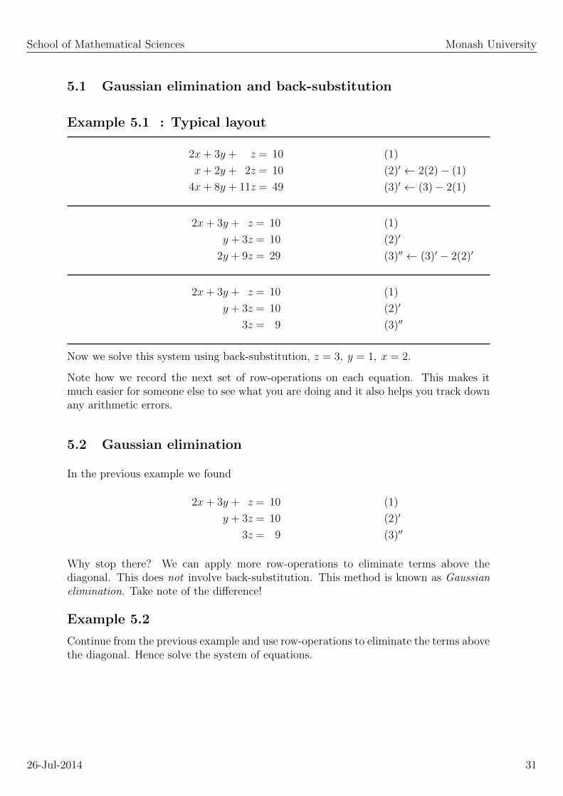
Example 5.1 : Typical layout
2x+ 3y + z = 10
x+ 2y + 2z = 10
4x+ 8y + 11z = 49
(1)
(2)′ ← 2(2)− (1)
(3)′ ← (3)− 2(1)
2x+ 3y + z = 10
y + 3z = 10
2y + 9z = 29
(1)
(2)′
(3)′′ ← (3)′ − 2(2)′
2x+ 3y + z = 10
y + 3z = 10
3z = 9
(1)
(2)′
(3)′′
Now we solve this system using back-substitution, z = 3, y = 1, x = 2.
Note how we record the next set of row-operations on each equation. This makes itmuch easier for someone else to see what you are doing and it also helps you track downany arithmetic errors.
5.2 Gaussian elimination
In the previous example we found
2x+ 3y + z = 10
y + 3z = 10
3z = 9
(1)
(2)′
(3)′′
Why stop there? We can apply more row-operations to eliminate terms above thediagonal. This does not involve back-substitution. This method is known as Gaussianelimination. Take note of the difference!
Example 5.2
Continue from the previous example and use row-operations to eliminate the terms abovethe diagonal. Hence solve the system of equations.
26-Jul-2014 31

School of Mathematical Sciences Monash University
5.2.1 Gaussian elimination strategy
1. Use row-operations to eliminate elements below the diagonal.
2. Use row-operations to eliminate elements above the diagonal.
3. If possible, re-scale each equation so that each diagonal element = 1.
4. The right hand side is now the solution of the system of equations.
If you bail out after step 1 you are doing Gaussian elimination with back-substitution(this is usually the easier option).
5.3 Exceptions
Here are some examples where problems arise.
Example 5.3 : A zero on the diagonal
2x + y + 2z + w = 2
2x + y − z + 2w = 1
x− 2y + z − w = −2
x + 3y − z + 2w = 2
(1)
(2)′ ← (2) − (1)
(3)′ ← 2(3)− (1)
(4)′ ← 2(4)− (1)
2x + y + 2z + w = 2
0y − 3z + w = −1
− 5y + 0z − 3w = −6
+ 5y − 4z + 3w = 2
(1)
(2)′′ ← (3)′
(3)′′ ← (2)′
(4)′
The zero on the diagonal on the second equation is a serious problem, it means we cannot use that row to eliminate the elements below the diagonal term. Hence we swap thesecond row with any other lower row so that we get a non-zero term on the diagonal.Then we proceed as usual. The result is w = 2, z = 1, y = 0 and x = −1.
Example 5.4
Complete the above example.
26-Jul-2014 32
School of Mathematical Sciences Monash University
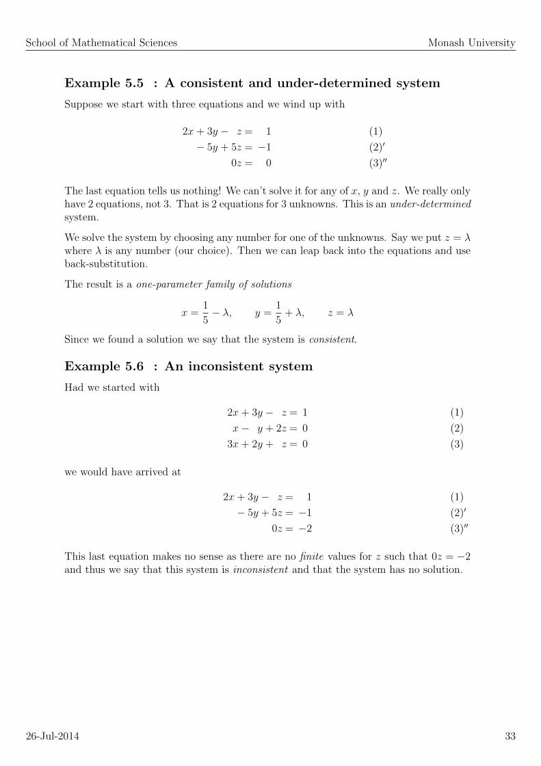
Example 5.5 : A consistent and under-determined system
Suppose we start with three equations and we wind up with
2x + 3y − z = 1
− 5y + 5z = −1
0z = 0
(1)
(2)′
(3)′′
The last equation tells us nothing! We can’t solve it for any of x, y and z. We really onlyhave 2 equations, not 3. That is 2 equations for 3 unknowns. This is an under-determinedsystem.
We solve the system by choosing any number for one of the unknowns. Say we put z = λwhere λ is any number (our choice). Then we can leap back into the equations and useback-substitution.
The result is a one-parameter family of solutions
x =1
5− λ, y =
1
5+ λ, z = λ
Since we found a solution we say that the system is consistent.
Example 5.6 : An inconsistent system
Had we started with
2x + 3y − z = 1
x− y + 2z = 0
3x + 2y + z = 0
(1)
(2)
(3)
we would have arrived at
2x + 3y − z = 1
− 5y + 5z = −1
0z = −2
(1)
(2)′
(3)′′
This last equation makes no sense as there are no finite values for z such that 0z = −2and thus we say that this system is inconsistent and that the system has no solution.
26-Jul-2014 33

SCHOOL OF MATHEMATICAL SCIENCES
ENG1091
Mathematics for Engineering
6. Matrices
School of Mathematical Sciences Monash University
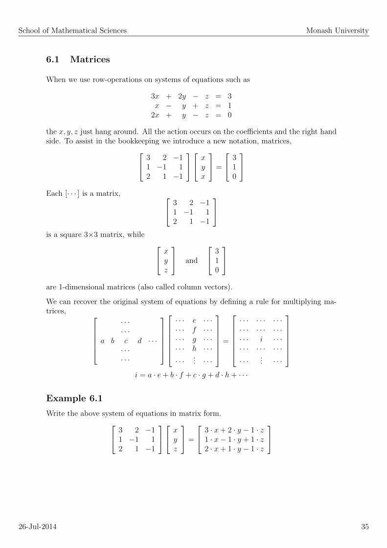
6.1 Matrices
When we use row-operations on systems of equations such as
3x + 2y − z = 3x − y + z = 1
2x + y − z = 0
the x, y, z just hang around. All the action occurs on the coefficients and the right handside. To assist in the bookkeeping we introduce a new notation, matrices, 3 2 −1
1 −1 12 1 −1
xyx
=
310
Each [· · · ] is a matrix, 3 2 −1
1 −1 12 1 −1
is a square 3×3 matrix, while x
yz
and
310
are 1-dimensional matrices (also called column vectors).
We can recover the original system of equations by defining a rule for multiplying ma-trices,
· · ·· · ·
a b c d · · ·· · ·· · ·
· · · e · · ·· · · f · · ·· · · g · · ·· · · h · · ·· · · ... · · ·
=
· · · · · · · · ·· · · · · · · · ·· · · i · · ·· · · · · · · · ·· · · ... · · ·
i = a · e+ b · f + c · g + d · h+ · · ·
Example 6.1
Write the above system of equations in matrix form. 3 2 −11 −1 12 1 −1
xyz
=
3 · x+ 2 · y − 1 · z1 · x− 1 · y + 1 · z2 · x+ 1 · y − 1 · z
26-Jul-2014 35

School of Mathematical Sciences Monash University
Example 6.2
Compute [2 34 1
] [1 70 2
]and
[1 70 2
] [2 34 1
]Note that we can only multiply matrices that fit together. That is, if A and B are a pairof matrices then in order that AB makes sense we must have the number of columns ofA equal to the number of rows of B.
Example 6.3
Does the following make sense?
[2 34 1
] 1 70 24 1
6.1.1 Notation
We use capital letters to represent matrices,
A =
3 2 −11 −1 12 1 −1
, X =
xyx
, B =
310
and our previous system of equations can then be written as
AX = B
Entries within a matrix are denoted by subscripted lowercase letters. Thus for the matrixB above we have b1 = 3, b2 = 1 and b3 = 0 while for the matrix A we have
A =
3 2 −11 −1 12 1 −1
=
a11 a12 a13
a21 a22 a23
a31 a32 a33
aij = the entry in row i and column j of A
To remind us that A is a square matrix with elements aij we sometimes write A = [aij].
6.1.2 Operations on matrices
I Equality :A = B
only when all entries in A equal those in B.
I Addition: Normal addition of corresponding elements.
26-Jul-2014 36

School of Mathematical Sciences Monash University
I Multiplication by a number : λA = λ times each entry of A
I Multiplication of matrices : ? ? ? ? ?
?????
=
?
I Transpose: Flip rows and columns, denoted by [· · · ]T .
[1 2 70 3 4
]T=
1 02 37 4
6.1.3 Some special matrices
I The Identity matrix :
I =
1 0 0 0 · · ·0 1 0 0 · · ·0 0 1 0 · · ·0 0 0 1 · · ·...
......
.... . .
For any square matrix A we have IA = AI = A.
I The Zero matrix : A matrix full of zeroes!
I Symmetric matrices : Any matrix A for which A = AT .
I Skew-symmetric matrices : Any matrix A for which A = −AT . Sometimes alsocalled anti-symmetric.
6.1.4 Properties of matrices
I AB 6= BA
I (AB)C = A(BC)
I (AT )T = A
I (AB)T = BTAT
26-Jul-2014 37

School of Mathematical Sciences Monash University
6.1.5 Notation
For the system of equations
3x + 2y − z = −1x − y + z = 4
2x + y − z = −1
we call 3 2 −11 −1 12 1 −1
the coefficient matrix and 3 2 −1 −1
1 −1 1 42 1 −1 −1
the augmented matrix.
When we do row-operations on a system we are manipulating the augmented matrix.But each incarnation represents a system of equations for the same original values forx, y and z. Thus if A and A′ are two augmented matrices for the same system, then wewrite
A ∼ A′
The squiggle means that even though A and A′ are not the same matrices, they do giveus the same values for x, y and z.
Example 6.4
Solve the system of equations
3x + 2y − z = −1x − y + z = 4
2x + y − z = −1
using matrix notation.
An accountant is someone who is good with numbers but lacks the personalityto be a statistician.
26-Jul-2014 38

SCHOOL OF MATHEMATICAL SCIENCES
ENG1091
Mathematics for Engineering
7. Inverses of Square Matrices.

School of Mathematical Sciences Monash University
7.1 Matrix Inverse
Suppose we have a system of equations[a bc d
] [xy
]=
[uv
]and that we write in the matrix form
AX = B
Can we find another matrix, call it A−1, such that
A−1A = I = the identity matrix
If so, then we have
A−1AX = A−1B ⇒ X = A−1B
Thus we have found the solution of the original system of equations.
For a 2× 2 matrix it is easy to verify that
A−1 =
[a bc d
]−1
=1
ad− bc
[d −b−c a
]
But how do we compute the inverse A−1 for other (square) matrices?
Here is one method.
7.1.1 Inverse by Gaussian elimination
I Use row-operations to reduce A to the identity matrix.
I Apply exactly the same row-operations to a matrix set initially to the identity.
I The final matrix is the inverse of A.
We usually record this process in a large augmented matrix.
I Start with [A|I].
I Apply row operations to obtain [I|A−1]
I Crack open the champagne.
26-Jul-2014 40
School of Mathematical Sciences Monash University
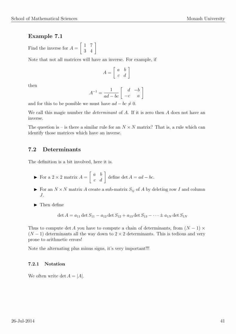
Example 7.1
Find the inverse for A =
[1 73 4
]Note that not all matrices will have an inverse. For example, if
A =
[a bc d
]then
A−1 =1
ad− bc
[d −b−c a
]and for this to be possible we must have ad− bc 6= 0.
We call this magic number the determinant of A. If it is zero then A does not have aninverse.
The question is – is there a similar rule for an N ×N matrix? That is, a rule which canidentify those matrices which have an inverse.
7.2 Determinants
The definition is a bit involved, here it is.
I For a 2× 2 matrix A =
[a bc d
]define detA = ad− bc.
I For an N×N matrix A create a sub-matrix Sij of A by deleting row I and columnJ .
I Then define
detA = a11 detS11 − a12 detS12 + a13 detS13 − · · · ± a1N detS1N
Thus to compute detA you have to compute a chain of determinants, from (N − 1) ×(N − 1) determinants all the way down to 2× 2 determinants. This is tedious and veryprone to arithmetic errors!
Note the alternating plus minus signs, it’s very important!!!
7.2.1 Notation
We often write detA = |A|.
26-Jul-2014 41
School of Mathematical Sciences Monash University
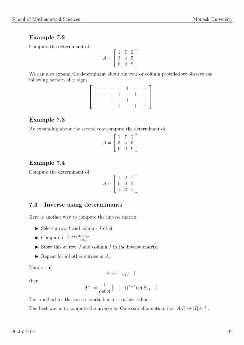
Example 7.2
Compute the determinant of
A =
1 7 23 4 56 0 9
We can also expand the determinant about any row or column provided we observe thefollowing pattern of ± signs.
+ − + − + − · · ·− + − + − + · · ·+ − + − + − · · ·− + − + − + · · ·
Example 7.3
By expanding about the second row compute the determinant of
A =
1 7 23 4 56 0 9
Example 7.4
Compute the determinant of
A =
1 2 70 0 31 2 1
7.3 Inverse using determinants
Here is another way to compute the inverse matrix.
I Select a row I and column J of A.
I Compute (−1)i+j detSIJdetA
I Store this at row J and column I in the inverse matrix.
I Repeat for all other entries in A.
That is , ifA = [ aIJ ]
then
A−1 =1
detA
[(−1)I+J detSJI
]This method for the inverse works but it is rather tedious.
The best way is to compute the inverse by Gaussian elimination, i.e. [A|I]→ [I|A−1].
26-Jul-2014 42
School of Mathematical Sciences Monash University
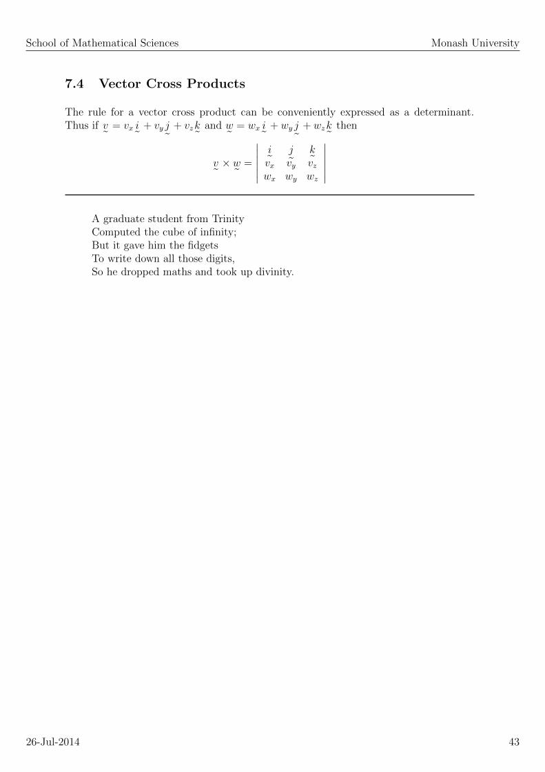
7.4 Vector Cross Products
The rule for a vector cross product can be conveniently expressed as a determinant.Thus if v
˜= vx i
˜+ vy j
˜+ vzk
˜and w
˜= wx i
˜+ wy j
˜+ wzk
˜then
v˜× w˜
=
∣∣∣∣∣∣i˜
j
˜k˜vx vy vz
wx wy wz
∣∣∣∣∣∣A graduate student from TrinityComputed the cube of infinity;But it gave him the fidgetsTo write down all those digits,So he dropped maths and took up divinity.
26-Jul-2014 43

SCHOOL OF MATHEMATICAL SCIENCES
ENG1091
Mathematics for Engineering
8. Eigenvalues and eigenvectors.
School of Mathematical Sciences Monash University
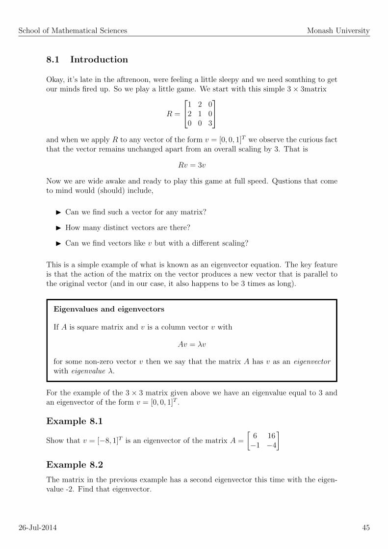
8.1 Introduction
Okay, it’s late in the aftrenoon, were feeling a little sleepy and we need somthing to getour minds fired up. So we play a little game. We start with this simple 3× 3matrix
R =
1 2 02 1 00 0 3
and when we apply R to any vector of the form v = [0, 0, 1]T we observe the curious factthat the vector remains unchanged apart from an overall scaling by 3. That is
Rv = 3v
Now we are wide awake and ready to play this game at full speed. Qustions that cometo mind would (should) include,
I Can we find such a vector for any matrix?
I How many distinct vectors are there?
I Can we find vectors like v but with a different scaling?
This is a simple example of what is known as an eigenvector equation. The key featureis that the action of the matrix on the vector produces a new vector that is parallel tothe original vector (and in our case, it also happens to be 3 times as long).
Eigenvalues and eigenvectors
If A is square matrix and v is a column vector v with
Av = λv
for some non-zero vector v then we say that the matrix A has v as an eigenvectorwith eigenvalue λ.
For the example of the 3 × 3 matrix given above we have an eigenvalue equal to 3 andan eigenvector of the form v = [0, 0, 1]T .
Example 8.1
Show that v = [−8, 1]T is an eigenvector of the matrix A =
[6 16−1 −4
]Example 8.2
The matrix in the previous example has a second eigenvector this time with the eigen-value -2. Find that eigenvector.
26-Jul-2014 45

School of Mathematical Sciences Monash University
Example 8.3
Let v1 and v2 be two eigenvectors of some matrix. Is it possible to choose α and β sothat αv1 + βv2 is also an eigenvector?
Now we can reexpress our earlier questions as follows.
I Does every matrix possess an eigenvector?
I How many eigenvalues can a matrix have?
I How do we compute the eigenvalues?
I Is this just pretty mathematics or is there a point to this game?
Good questions indeed. Let’s see what we make of them. We will start with the issueof constructing the eigenvalues (assuming, for the moment, that they exist).
8.2 Eigenvalues
Our game here is to find the non-zero values of λ, if any, that allows the equation
Av = λv
to have non-zero solutions for v. Take that is given, then re-arrange the equation to
(A− λI) v = 0
where I is the identity matrix (of the same shape as A). Since we are chasing non-zerosolutions for v we must have the determinant of A − λI equal to zero. That is, werequire that 0 = det(A − λI). This is a polynomial equation in λ and is known as thecharacteristic equation for λ.
Characteristic equation
The eigenvalues λ of a matrix A are solutions of the polynomial equation
0 = det(A− λI)
This is called the characteristic equation of A. If A is an N ×N matrix, then thisequation will be a polynomial of degree N in λ. The eigenvalues may in general becomplex numbers.
26-Jul-2014 46
School of Mathematical Sciences Monash University
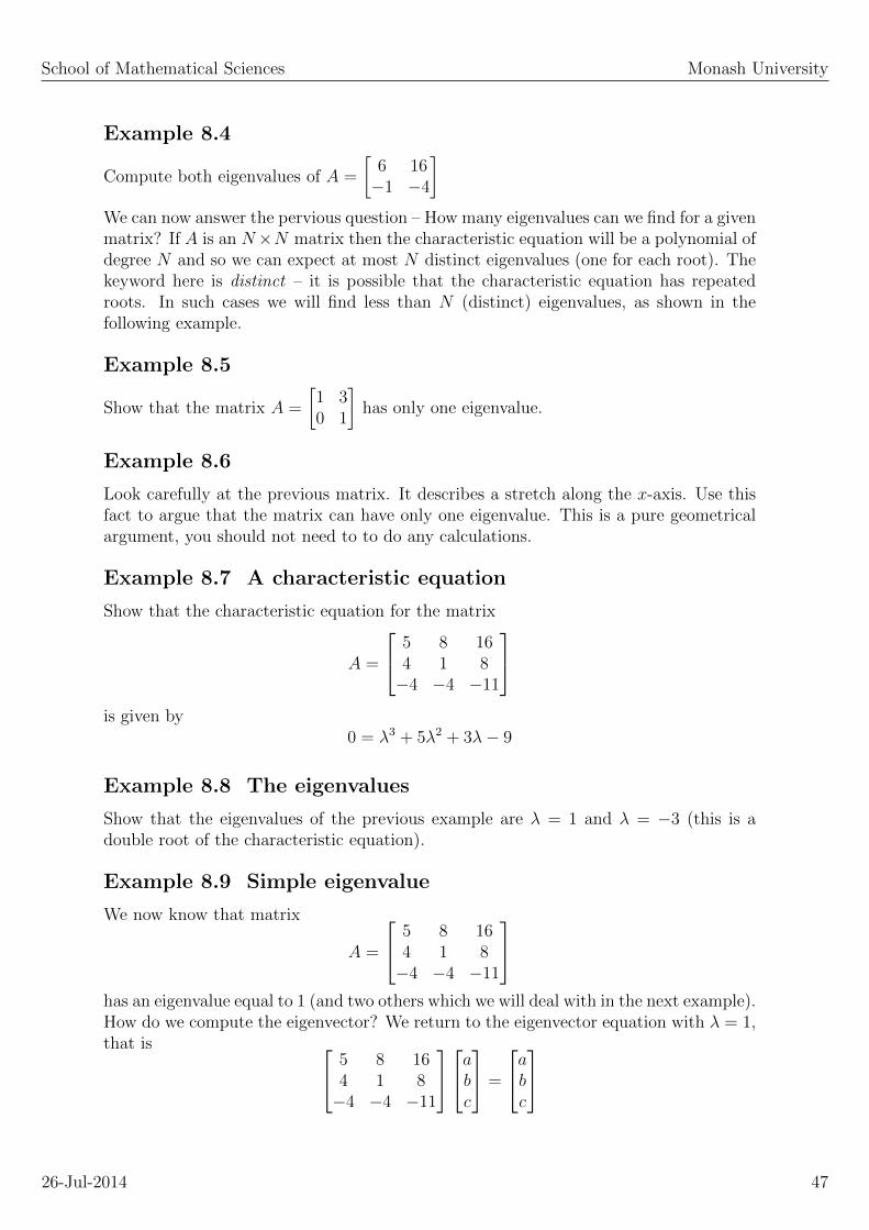
Example 8.4
Compute both eigenvalues of A =
[6 16−1 −4
]We can now answer the pervious question – How many eigenvalues can we find for a givenmatrix? If A is an N×N matrix then the characteristic equation will be a polynomial ofdegree N and so we can expect at most N distinct eigenvalues (one for each root). Thekeyword here is distinct – it is possible that the characteristic equation has repeatedroots. In such cases we will find less than N (distinct) eigenvalues, as shown in thefollowing example.
Example 8.5
Show that the matrix A =
[1 30 1
]has only one eigenvalue.
Example 8.6
Look carefully at the previous matrix. It describes a stretch along the x-axis. Use thisfact to argue that the matrix can have only one eigenvalue. This is a pure geometricalargument, you should not need to to do any calculations.
Example 8.7 A characteristic equation
Show that the characteristic equation for the matrix
A =
5 8 164 1 8−4 −4 −11
is given by
0 = λ3 + 5λ2 + 3λ− 9
Example 8.8 The eigenvalues
Show that the eigenvalues of the previous example are λ = 1 and λ = −3 (this is adouble root of the characteristic equation).
Example 8.9 Simple eigenvalue
We now know that matrix
A =
5 8 164 1 8−4 −4 −11
has an eigenvalue equal to 1 (and two others which we will deal with in the next example).How do we compute the eigenvector? We return to the eigenvector equation with λ = 1,that is 5 8 16
4 1 8−4 −4 −11
abc
=
abc
26-Jul-2014 47
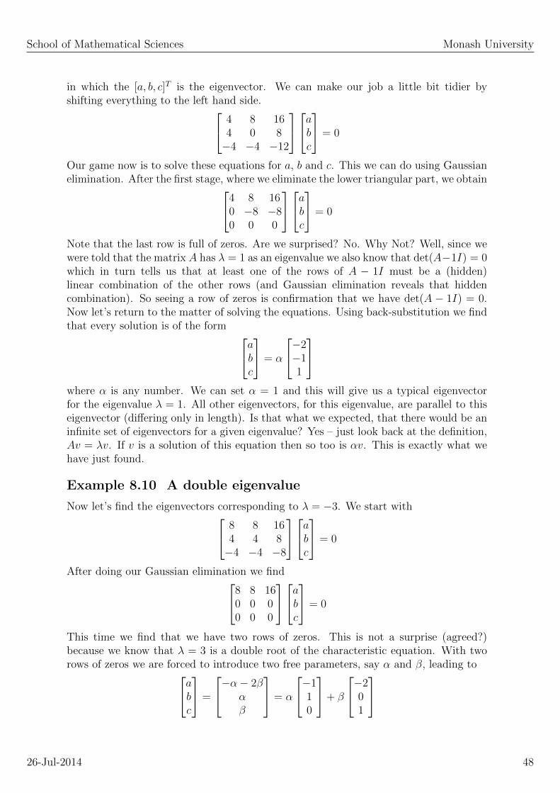
School of Mathematical Sciences Monash University
in which the [a, b, c]T is the eigenvector. We can make our job a little bit tidier byshifting everything to the left hand side. 4 8 16
4 0 8−4 −4 −12
abc
= 0
Our game now is to solve these equations for a, b and c. This we can do using Gaussianelimination. After the first stage, where we eliminate the lower triangular part, we obtain4 8 16
0 −8 −80 0 0
abc
= 0
Note that the last row is full of zeros. Are we surprised? No. Why Not? Well, since wewere told that the matrix A has λ = 1 as an eigenvalue we also know that det(A−1I) = 0which in turn tells us that at least one of the rows of A − 1I must be a (hidden)linear combination of the other rows (and Gaussian elimination reveals that hiddencombination). So seeing a row of zeros is confirmation that we have det(A − 1I) = 0.Now let’s return to the matter of solving the equations. Using back-substitution we findthat every solution is of the form ab
c
= α
−2−11
where α is any number. We can set α = 1 and this will give us a typical eigenvectorfor the eigenvalue λ = 1. All other eigenvectors, for this eigenvalue, are parallel to thiseigenvector (differing only in length). Is that what we expected, that there would be aninfinite set of eigenvectors for a given eigenvalue? Yes – just look back at the definition,Av = λv. If v is a solution of this equation then so too is αv. This is exactly what wehave just found.
Example 8.10 A double eigenvalue
Now let’s find the eigenvectors corresponding to λ = −3. We start with 8 8 164 4 8−4 −4 −8
abc
= 0
After doing our Gaussian elimination we find8 8 160 0 00 0 0
abc
= 0
This time we find that we have two rows of zeros. This is not a surprise (agreed?)because we know that λ = 3 is a double root of the characteristic equation. With tworows of zeros we are forced to introduce two free parameters, say α and β, leading toab
c
=
−α− 2βαβ
= α
−110
+ β
−201
26-Jul-2014 48
School of Mathematical Sciences Monash University
This shows that every eigenvector for λ = −3 is a linear combination of the pair ofvectors [−1, 1, 0]T and [−2, 0, 1]T .
Example 8.11
Show that eigenvectors of the previous example can also be constructed from linearcombinations of [−1, 1, 0]T and [1, 1,−1]T .
8.3 Decomposing Symmetric matrices
Earlier on we asked what is the point of computing eigenvectors and eigenvalues (otherthan pure fun)? Here we will develop some really nice results that follow once we knowthe eigenvalues and eigenvectors. Though many of the results we are about to explorealso apply to general square matrices they are much easier to present (and prove) forreal symmetric matrices that posses a complete set of eigenvalues (i.e. no multiple rootsin the characteristic equation). This restriction is not so severe as to be meaningless formany of the matrices encountered in mathematical physics (and other fields) are oftenof this class.
Real symmetric matrices with complete eigenvalues
If A is an N × N real symmetric matrix with N distinct eigenvalues λi, i =1, 2, 3 · · ·N with corresponding eigenvectors vi, i = 1, 2, 3 · · ·N then
I The eigenvalues are real, λi = λ̄i, i = 1, 2, 3 · · ·N and
I The eigenvectors for distinct eigenvalues are orthogonal, vTi vj = 0, i 6= j.
We will only prove the first of these theorems, the second is left as an example for youto play with (it is not all that hard).
We start by constructing v̄TAv (where the bar over the v means complex conjugation).This is just one number, that is a 1× 1 matrix. Thus it equals its own transpose. So wehave
v̄TAv =(v̄TAv
)Tnow use (BC)T = (CB)T
= (Av)T v̄ and again
= vTAT v̄ but AT = A
= vTAv̄
Now from the definition Av = λv we also have, by taking complex conjugates and notingthat A is real, Av̄ = λ̄v̄. Substitute this into the previous equation to obtain
v̄TAv = vT λ̄v̄ = λ̄vT v̄
26-Jul-2014 49
School of Mathematical Sciences Monash University
But look now at the left hand side. We can manipulate this as follows
v̄TAv = v̄T (Av)
= v̄Tλv
= λv̄Tv
Compare this with our previous equation and you will see that we must have
λv̄Tv = λ̄vT v̄
Finally we notice that vT v̄ = v̄Tv = v21 + v2
2 + v23 · · · v2
N 6= 0. So this leaves just
λ̄ = λ
Our job is done, we have proved that the eigenvalue must be real.
Now here comes a very nice result. We will work with a simple 3 × 3 real symmetricmatrix with 3 distinct eigenvalues simply to make the notation less cluttered than wouldbe the case if we leapt straight into the general N×N case. We will have 3 eigenvalues α,β and γ. The corresponding eigenvectors will be u, v and w. Each eigenvector containsthree numbers, so we will write v = [v1, v2, v3]T etc. We are free to stretch or shrink eacheigenvector so let us assume that they have been scaled so that each is a unit vector,i.e. vTv = 1 etc. Now let’s assemble the three separate eigenvalue equations into onebig matrix equation, like this
A
u1 v1 w1
u2 v2 w2
u3 v3 w3
=
u1 v1 w1
u2 v2 w2
u3 v3 w3
α 0 00 β 00 0 γ
This looks pretty but what can we do with this? Good question. The big trick is that wecan easily (trust me) solve this set of equations for the matrix A. Really? Let’s supposethat the 3 × 3 matrix to the right of A has an inverse. Then we could solve for A bymultiplying by the inverse from the left, to obtain
A =
u1 v1 w1
u2 v2 w2
u3 v3 w3
α 0 00 β 00 0 γ
u1 v1 w1
u2 v2 w2
u3 v3 w3
−1
This is nice, but can we compute the inverse? In fact we already have it, just lookcarefully at this equationu1 u2 u3
v1 v2 v3
w1 w2 w3
u1 v1 w1
u2 v2 w2
u3 v3 w3
=
1 0 00 1 00 0 1
This is just a simple way of stating that the eigenvectors are orthogonal and of unitlength. This also shows that one matrix is the inverse of the other, that isu1 v1 w1
u2 v2 w2
u3 v3 w3
−1
=
u1 u2 u3
v1 v2 v3
w1 w2 w3
26-Jul-2014 50
School of Mathematical Sciences Monash University
Now we have our final result
A =
u1 v1 w1
u2 v2 w2
u3 v3 w3
α 0 00 β 00 0 γ
u1 u2 u3
v1 v2 v3
w1 w2 w3
This shows that any real symmetric 3 × 3 matrix, with three distinct eigenvalues, canbe re-built from its eigenvalues and eigenvectors. This is not only a neat result it is alsoan extremely useful result.
In the following examples we will assume that the matrix A is a real symmetric 3 × 3matrix with three distinct eigenvalues.
Example 8.12
Use the above expansion for A to compute A2, A3, A4 and so on.
Example 8.13
Use the definition of an eigenvalue to show that A2 has an eigenvalue α2, A3 an eigenvalueα3 and so on. How does this compare with the previous example?
Example 8.14
Suppose that λ is an eigenvalue, with corresponding eigenvector v, of any square matrixB. Can you construct an eigenvalue and eigenvector for B−1 (assuming that the inverseexists)?
8.4 Matrix inverse
The past few examples shows, for our general class of real symmetric 3× 3 matrices A,with three distinct eigenvalues, that the powers of A can be written as
An =
u1 v1 w1
u2 v2 w2
u3 v3 w3
αn 0 00 βn 00 0 γn
u1 u2 u3
v1 v2 v3
w1 w2 w3
It is easy to see that this is true for any positive integer n. But it also applies (assumingα, β and γ are non-zero) when n is a negative integer. How can we be so sure? Weknow that A and A−1 share the same eigenvectors. Good. We also know that if α is aneigenvalue of A then 1/α is an eigenvalue of A−1. Finally we note that A−1, like A, is areal symmetric 3 × 3 matrix with three (non-zero) distinct eigenvalues. Since we knowall of its eigenvalues and eigenvectors we can use the eigenvalue expansion to write A−1
as
A−1 =
u1 v1 w1
u2 v2 w2
u3 v3 w3
α−1 0 00 β−1 00 0 γ−1
u1 u2 u3
v1 v2 v3
w1 w2 w3
26-Jul-2014 51

School of Mathematical Sciences Monash University
Which is just what we would have got by putting n = −1 in the previous equation.From here we could compute A−2 = A−1A−1, A−3 = A−1A−2 and so on. In short, wehave proved the above expression for An for any integer n, positive or negative.
The above result (with n = −1) give us yet another way to compute the inverse of A.Isn’t this exciting (and unexpected)?
8.5 The Cayley-Hamilton theorem: Not examinable
What do we know about the three eigenvalues α, β and γ? We know that they aresolutions of the characteristic polynomial
0 = det(A− λI)
which, after some simple algebra, leads to a polynomial of the form
0 = λ3 + b1λ2 + b2λ
1 + b3λ0
where b1, b2 and b3 are some numbers (built from the numbers in A).
Now let’s do something un-expected (expect the un-expected). Let’s replace the numberλ with the 3 × 3 matrix A in the right hand side of the above polynomial. Where weencounter the powers of A we will use what we have learnt above, that we can useexpansions in powers of the eigenvalues. Thus we have
A3 + b1A2 + b2A+ b3I =
u1 v1 w1
u2 v2 w2
u3 v3 w3
α3 0 00 β3 00 0 γ3
u1 u2 u3
v1 v2 v3
w1 w2 w3
+ b1
u1 v1 w1
u2 v2 w2
u3 v3 w3
α2 0 00 β2 00 0 γ2
u1 u2 u3
v1 v2 v3
w1 w2 w3
+ b2
u1 v1 w1
u2 v2 w2
u3 v3 w3
α1 0 00 β1 00 0 γ1
u1 u2 u3
v1 v2 v3
w1 w2 w3
+ b3
u1 v1 w1
u2 v2 w2
u3 v3 w3
α0 0 00 β0 00 0 γ0
u1 u2 u3
v1 v2 v3
w1 w2 w3
We can tidy this up by collecting the eigenvalue terms into one matrix
A3 + b1A2 + b2A+ b3I =
u1 v1 w1
u2 v2 w2
u3 v3 w3
D11 0 00 D22 00 0 D33
u1 u2 u3
v1 v2 v3
w1 w2 w3
where
D11 = α3 + b1α2 + b2α + b3
D22 = β2 + b1β2 + b2β + b3
D33 = γ3 + b1γ2 + b2γ + b3
26-Jul-2014 52
School of Mathematical Sciences Monash University
However we know that each eigenvalue is a solution of the polynomial equation
0 = λ3 + b1λ2 + b2λ+ b3
which means that D11 = D22 = D33 = 0 and thus the middle matrix is in fact the zeromatrix. Thus we have shown that
0 = A3 + b1A2 + b2A+ b3I
This is an example of the Cayley-Hamilton theorem. It is very much un-expected(agreed?).
It has been a long road but the journey was fun (yes it was) and it has lead us to afamous theorem in the theory of matrices, the Cayley-Hamilton theorem. Though wehave demonstrated the theorem for the particular case of real symmetric matrices withdistinct eigenvalues it, the theorem, happens to be true for any square matrix. Provingthat this is so is far from easy but sadly the margins of this textbook are too narrow torecord the proof, you will have to wait until your second year of maths.
The Cayley-Hamilton theorem
Let A be any N ×N matrix. Then define the polynomial P (λ) by
P (λ) = det(A− λI)
where I is the N ×N identity matrix. Then
0 = P (A)
Note that the eigenvalues λ of A are the solutions of
0 = P (λ)
26-Jul-2014 53

SCHOOL OF MATHEMATICAL SCIENCES
ENG1091
Mathematics for Engineering
9. Hyperbolic functions

School of Mathematical Sciences Monash University
9.1 Hyperbolic functions
Do you remember the time when you first encountered the sine and cosine functions?That would have been in early secondary school when you were studying trigonometry.These functions proved very useful when faced with problems to do with triangles. Youmay have been surprised when (many years later) you found that those same functionsalso proved useful when solving some integration problems. Here is a classic example.
Example 9.1 Integration requiring trigonometric functions
Evaluate the following anti-derivative
I =
∫1√
1− x2dx
We will use a substitution, x(u) = sinu, as follows
I =
∫1√
1− x2dx put x = sinu and dx = cosu du
=
∫1
cosucosu du
=
∫du
and thus ∫1√
1− x2dx = sin−1 x
where, for simplicity, we have ignored the usual integration constant.
This example was very simple and contained nothing new. But if we had been given thefollowing integral
I =
∫1√
1 + x2dx
and continued to use a substitution based on simple sine and cosine functions thenwe would find the game to be rather drawn out. As you can easily verify, the correctsubstitution is x(u) = tanu and the integration (ignoring integration constants) leadsto ∫
1√1 + x2
dx = loge
(x+√
1 + x2)
26-Jul-2014 55

School of Mathematical Sciences Monash University
Example 9.2
Verify the above integration.
This situation is not all that satisfactory as it involve a series of tedious substitutionsand takes far more work than the first example. Can we do a better job? Yes, butit involves a trick where we define new functions, known as hyperbolic functions, to doexactly that job.
For the moment we will leave behind the issue of integration and focus on this new classof functions. Later we will return to our integrals to show how easy the job can be.
9.1.1 Hyperbolic functions
The hyperbolic functions are rather easy to define. It all begins with this pair of functionssinhu, known as hyperbolic sine and pronounced either as sinch or shine and coshu,known as hyperbolic cosine and pronounced as cosh. They are defined by
sinhu =1
2
(eu − e−u
)coshu =
1
2
(eu + e−u
)|u| <∞
These functions bare names similar to sin and cos for the simple reason that they shareproperties similar to those of sin and cos (as we will soon see).
The above definitions for sinh and cosh are really all you need to know – everything elseabout hyperbolic functions follows form these two definitions. Of course it does not hurtto commit to memory some of the equations we are about to present.
Here are a few elementary properties of sinh and cosh You can easily verify that
cosh2 u− sinh2 u = 1
d coshu
du= sinhu ,
d sinhu
du= coshu
Here is a more detailed list of properties (which of course you will verify, by using theabove definitions).
Properties of Hyperbolic functions. Pt.1
cosh2 x− sinh2 x = 1
cosh(u+ v) = coshu cosh v + sinhu sinh v
sinh(u− v) = sinhu cosh v − sinh v coshu
2 cosh2 x = 1 + cosh(2x) , 2 sinh2 x = −1 + cosh(2x)
d coshx
dx= sinhx ,
d sinhx
dx= coshx
26-Jul-2014 56

School of Mathematical Sciences Monash University
x
cosh,sinh
cosh(x)
sinh(x)
−3 −2 −1 0 1 2 3
−10
−5
05
10
This looks very pretty and reminds us (well it should remind us) of remarkably similarproperties for the sin and cos functions. Now recall the promise we gave earlier, thatthese hyperbolic functions would make our life with certain integrals much easier. So letus return to the integral from earlier in this chapter. Using the same layout and similarsentences here is how we would complete the integral using our new found friends.
Example 9.3 Integration requiring hyperbolic functions
Evaluate the following anti-derivative
I =
∫1√
1 + x2dx
We will use a substitution, x(u) = sinhu, as follows
I =
∫1√
1 + x2dx put x = sinhu and dx = coshu du
=
∫1
coshucoshu du
=
∫du
and thus ∫1√
1 + x2dx = sinh−1 x
where, for simplicity, we have ignored the usual integration constant.
9.1.2 More hyperbolic functions
You might be wondering if there are hyperbolic equivalents to the familiar trigonometricfunctions tan, cotan, sec and cosec. Good question, and yes, indeed there are equivalents
26-Jul-2014 57

School of Mathematical Sciences Monash University
named tanh, cotanh, sech and cosech. The following table provides some basic facts(which again you should verify).
Properties of Hyperbolic functions. Pt.2
tanhx =sinhx
coshxcotanhx =
coshx
sinhx
sechx =1
coshxcosechx =
1
sinhx
sech2 x− tanh2 x = 1
d tanhx
dx= sech2 x ,
d cotanhx
dx= − cosech2 x
9.2 Special functions: not examinable
In the previous examples we conveniently ignored the integration constants. But weshould not be so flippant, instead we should have written
sinh−1 x = C +
∫ x
0
1√1 + u2
du
Note that the integral on the right hand side vanishes when x = 0 and thus C =sinh−1(0). The good thing is that we know that sinh(0) = 0 and this fact can be usedto properly determine the integration constant, that is C = 0 and thus we have
sinh−1 x =
∫ x
0
1√1 + u2
du
Now we come to an interesting re-interpretation. We could have begun our discussionson hyperbolic sine from this very equation. That is, we could use the right hand sideto define the (inverse) hyperbolic sine. But now you might ask: How do we computea number for sinh−1(0.45)? One method would be to compute an approximation byestimating the area under the curve. A better method is to evaluate the right hand sideusing loge(x +
√1 + x2) as the anti-derivative. Either way it is a bit messy but it does
establish the point, that this integral contains everything we could ever wish to knowabout sinh−1.
What is the point of this discussion? Well it shows how we can turn adversity intoadvantage. Where previously we had a difficult integral (not impossible but difficultnone the less) we invented new functions (the hyperbolic functions) that made suchintegrals trivial. The same idea can be applied to many many more integrals. Forexample, the following integral
erf(x) =2√π
∫ x
0
e−u2
du
26-Jul-2014 58

School of Mathematical Sciences Monash University
defines a special function known as the error function. It is used extensively in statisticsand diffusion problems (such as the flow of heat). For this integral there is no knownanti-derivative and thus values for erf(x) can only be obtained by some other means(e.g., the area under the graph).
Euclid’s fashion tip: When attending Hyperbolic Functions always choose neat andcasual.
26-Jul-2014 59

SCHOOL OF MATHEMATICAL SCIENCES
ENG1091
Mathematics for Engineering
10. Integration

School of Mathematical Sciences Monash University
10.1 Integration : Revision
Computing I =∫f(x)dx is no different from finding the function F (x) such that
dF/dx = f(x).
The function F (x) is called the anti-derivative of f(x). Finding F (x) can be very tricky.
Example 10.1
I =
∫sinx dx
This means find the function F (x) such that
dF (x)
dx= sinx
We know this to be F (x) = − cosx+ C where C is a constant of integration.
Example 10.2
I =
∫sin(3x) dx
For this we use a substitution,
u = 3x , ⇒ du = 3dx , ⇒ dx =du
3
Thus we have
I =
∫sin(3x) dx =
∫(sinu)
(1
3du
)=
1
3
∫sinu du
=1
3(− cosu) + C
Now we flip back to the variable x,
I =
∫sin(3x) dx = −1
3cos(3x) + C
Example 10.3
I =
∫x exp(x2) dx
Choose a substitution that targets the ugly bit in the integral. Thus put u(x) = x2.Then du = 2xdx and xdx = du/2. This gives us
I =
∫1
2exp(u) du =
1
2expu+ C =
1
2exp(x2) + C
26-Jul-2014 61
School of Mathematical Sciences Monash University
10.1.1 Some basic integrals
You must remember the following integrals.∫exp(x) dx = exp(x) + C
∫cos(x) dx = sin(x) + C
∫sin(x) dx = − cos(x) + C
∫xn dx =
1
n+ 1xn+1, n 6= −1
∫1
xdx = log(x) + C
10.1.2 Substitution
If I =∫f(x) dx looks nasty, try changing the variable of integration. That is put
u = u(x) for some chosen function u(x) (usually inspired by some part of f(x)). Thenwe invert the function to find x = x(u) and substitute into the integral.
I =
∫f(x) dx =
∫f(x(u))
dx
dudu
If we have chosen well, then this second integral will be easy to do.
10.2 Integration by parts
This is a very powerful technique based upon the product rule for derivatives.
Recall thatd(fg)
dx= g
df
dx+ f
dg
dx
Now integrate both sides∫d(fg)
dxdx =
∫gdf
dxdx+
∫fdg
dxdx
But integration is the inverse of differentiation, thus we have
fg =
∫gdf
dxdx+
∫fdg
dxdx
26-Jul-2014 62

School of Mathematical Sciences Monash University
which we can re-arrange to ∫fdg
dxdx = fg −
∫gdf
dxdx
Thus we have converted one integral into another. The hope is that the second integralis easier than the first. This will depend on the choices we make for f and dg/dx.
Example 10.4
I =
∫x exp(x) dx
We have to split the integrand x exp(x) into two pieces, f and dg/dx.
Choosef(x) = x ⇒ df
dx= 1
dgdx
= exp(x) ⇒ g(x) = exp(x)
Then
I =
∫x exp(x) dx = fg −
∫gdf
dxdx
= x exp(x)−∫
1 · exp(x) dx
= x exp(x)− exp(x) + C
Example 10.5
I =
∫x cos(x) dx
Choosef(x) = x ⇒ df
dx= 1
dgdx
= cos(x) ⇒ g(x) = sin(x)
and thus
I =
∫x cos(x) dx = x sin(x)−
∫1 · sin(x) dx
= x sin(x) + cos(x) + C
26-Jul-2014 63
School of Mathematical Sciences Monash University
Example 10.6
I =
∫x log(x) dx
Choosef(x) = x ⇒ df
dx= 1
dgdx
= log(x) ⇒ g(x) =???
We don’t know immediately the anti-derivative for log(x), so we try another split. Thistime we choose
f(x) = log(x) ⇒ dfdx
= 1x
dgdx
= x ⇒ g(x) = 12x2
and this leads to
I =
∫x log(x) dx =
1
2x2 log(x)−
∫1
2x2 1
xdx
=1
2x2 log(x)− 1
4x2 + C
Example 10.7
Evaluate
I =
∫log(x)
xdx
Two students were doing a maths test. The answer to the the first questionwas log(1 + x). A weak student copied the answer from a good student,but didn’t want to make it obvious that he was cheating, so he changed theanswer slightly, to timber(1 + x).
26-Jul-2014 64

SCHOOL OF MATHEMATICAL SCIENCES
ENG1091
Mathematics for Engineering
11. Improper integrals

School of Mathematical Sciences Monash University
11.1 Improper Integrals
When a definite integral contains an infinity, either in the integrand or on the limits, wesay that we have an improper integral. All other integrals are proper integrals.
Example 11.1
I =
∫ 1
0
dx√x
, I =
∫ ∞0
dx
1 + x2
I =
∫ 1
−1
dx
x2, I =
∫ π/2
0
tan(x) dx
Because of the infinity we must treat the improper integral with care.
11.1.1 A standard strategy
We construct a related proper integral say I(ε) that depends on a parameter ε. Wechoose I(ε) such that we recover the original integral as a limit, say as ε→ 0.
Example 11.2
I =
∫ 1
0
dx√x
For this we construct a related proper integral
I(ε) =
∫ 1
ε
dx√x
ε > 0
Since this is a proper integral for ε > 0 we can evaluate it directly,
I(ε) =
∫ 1
ε
dx√x
=[2√x]1ε
= 2− 2√ε
Next we evaluate the limit as ε→ 0
limε→0
I(ε) = limε→0
2− 2√ε = 2
As this answer is well defined (i.e. finite and independent of the way the limit is ap-proached) we are justified in defining this to be the value of the improper integral.
I =
∫ 1
0
dx√x
= limε→0
∫ 1
ε
dx√x
= 2
26-Jul-2014 66

School of Mathematical Sciences Monash University
In this case we say we have a convergent improper integral. Had we not got a finiteanswer we would say that we had an divergent improper integral.
Example 11.3
I =
∫ 1
0
dx
x2
This time we choose
I(ε) =
∫ 1
ε
dx
x2ε > 0
which we can easily evaluate
I(ε) =1
ε− 1
and thus
limε→0
I(ε) =∞
This is not finite so this time we say the the improper integral is a divergent improperintegral.
Example 11.4
What do you think of the following calculation? Be warned : the answer is wrong!
I =
∫ 1
−1
dx
x2=
[−1
x
]1
−1
= −2
Example 11.5
I =
∫ 1
−1
dx
x3
This time we have an improper integral because the integrand is singular inside theregion of integration. We create our related proper integral by cutting out the singularpoint. Thus we define two separate proper integrals,
26-Jul-2014 67

School of Mathematical Sciences Monash University
I1(η) =
∫ −η−1
dx
x3dx η > 0
I2(ε) =
∫ 1
ε
dx
x3dx ε > 0
If both I1 and I2 converge (i.e. have finite values) we say that I also converges with thevalue
I = limη→0
I1(η) + limε→0
I2(ε)
But for our case
I1(η) = 1− 1
η2⇒ lim
η→0I1(η) = −∞
I2(ε) = −1 +1
ε2⇒ lim
ε→0I2(ε) = +∞
Thus neither I1 nor I2 converges and thus I is a divergent improper integral.
This may seem easy (it is) but it does require some care as the next example shows.
Example 11.6
Suppose we chose I1 and I2 as before but we set
ε =η√
1 + 2η2⇒ 1
ε2− 1
η2= 2
Then we would find that
I1(η) + I2(ε) =
(1
ε2− 1
η2
)= 2
for all η > 0 and therefore
limη→0
I1 + I2 = 2
But had we chosen
ε = η
26-Jul-2014 68

School of Mathematical Sciences Monash University
we would have found that
limη→0
I1 + I2 = 0
How can this be? The answer is that in computing I1 + I2 we are eventually trying tomake sense of −∞+∞. Depending on how we approach the limit we can get any answerwe like for −∞+∞.
Consequently, when we say that an integral is divergent we mean that either its valueis infinity or that it has no single well defined value.
A father who is very much concerned about his son’s bad grades in mathsdecides to register him at a catholic school. After his first term there, the sonbrings home his report card: He’s getting ”A”s in maths. The father is, ofcourse, pleased, but wants to know: ”Why are your maths grades suddenlyso good?” ”You know”, the son explains, ”the first day when I walked intothe classroom, I instantly that this place means business!” And why was thatinquired the father. ”Dad! they’ve got a guy hanging on the wall and they’venailed him to a plus sign!” exclaimed his son.
26-Jul-2014 69
SCHOOL OF MATHEMATICAL SCIENCES
ENG1091
Mathematics for Engineering
12. Comparison test for convergence

School of Mathematical Sciences Monash University
12.1 Comparison Test for Improper Integrals
Example 12.1
I =
∫ ∞2
e−x2
dx
For this integral we would choose
I(ε) =
∫ ε
2
e−x2
dx
and provided that the limit exists, we would write
I = limε→∞
I(ε)
The trouble is we do not have a simple anti-derivative for e−x2. The trick here is to look
at a simpler (improper) integral for which we can find a simple anti-derivative.
Note that
0 < e−x2
< e−x for 2 < x <∞
Now integrate
0 <
∫ ε
2
e−x2
dx <
∫ ε
2
e−x dx
and the last integral on the right is easy to do (thats one reason why we chose e−x),
0 <
∫ ε
2
e−x2
dx <
∫ ε
2
e−x dx = e−2 − e−ε
Our next step is take the limit as ε→∞
0 < limε→∞
∫ ε
2
e−x2
dx < limε→∞
e−2 − e−ε = e−2
The limit exists and is finite so we have our final answer that I =∫∞
2e−x
2dx is
convergent.
26-Jul-2014 71

School of Mathematical Sciences Monash University
Example 12.2
I =
∫ 1
0
ex
xdx and I(ε) =
∫ 1
ε
ex
xdx
Again we do not have a simple anti-derivative for ex/x so we study a related integral
J =
∫ 1
0
1
xdx and J(ε) =
∫ 1
ε
1
xdx
For each integral the appropriate limit is ε→ 0.
Now we proceed as follows
0 <1
x<ex
xfor 0 < x < 1
⇒ 0 <
∫ 1
ε
1
xdx <
∫ 1
ε
ex
xdx
⇒ 0 < log 1− log ε < I(ε)
Now we take the limit, in this case, ε→ 0,
0 < limε→0
(log 1− log ε) < limε→0
I(ε)
⇒ 0 <∞ < limε→0
I(ε)
Thus we conclude that I =∫ 1
0ex/x dx is divergent.
Example 12.3
I =
∫ 1
0
ex
xdx and I(ε) =
∫ 1
ε
ex
xdx
Suppose (mistakenly) we thought that this integral converged. We might set out toprove this by starting with
0 <ex
x<
3
xfor 0 < x < 1
then we would leap into the now familiar steps,
26-Jul-2014 72

School of Mathematical Sciences Monash University
0 <
∫ 1
ε
ex
xdx <
∫ 1
ε
3
xdx = 3(log 1− log ε)
⇒ 0 < limε→0
∫ 1
ε
ex
xdx < lim
ε→03(log 1− log ε) =∞
⇒ 0 < limε→0
I(ε) <∞
This last line tells us nothing. Though we set out to prove convergence we actuallyproved nothing. Thus either we were wrong in supposing that the integral converged orwe made a bad choice for the test function 3/x. We know from the previous examplethat in fact this integral is divergent.
12.2 The General Strategy
Suppose we have ∫ ∞0
f(x) dx with f(x) > 0
Then we have two cases to consider.
I Test for convergence If you can find c(x) such that
(1) 0 < f(x) < c(x) and(2) limε→∞
∫ ε0c(x) dx is finite.
then I is convergent.
26-Jul-2014 73

School of Mathematical Sciences Monash University
I Test for divergence If you can find d(x) such that
(1) 0 < d(x) < f(x) and(2) limε→∞
∫ ε0d(x) dx =∞.
then I is divergent.
We generally try to choose the test function (c(x) or d(x)) so that it has a simpleanti-derivative.
A strategy similar to the above would apply for integrals like I =∫ 1
0f(x) dx.
Example 12.4
Re-write the above strategy for the case I =∫ 1
0f(x) dx.
A mathematician named KleinThought the Mobius band was divineSaid he: If you glueThe edges of twoYou’ll get a weird bottles like mine.
26-Jul-2014 74

SCHOOL OF MATHEMATICAL SCIENCES
ENG1091
Mathematics for Engineering
13. Introduction to sequences and series.

School of Mathematical Sciences Monash University
13.1 Definitions
I Sequence. A set of numbers such as
1, 12, 1
3, 1
4, 1
5, · · ·
1, −12, 1
3, −1
4, 1
5, · · ·
1, 14, 1
9, 1
16, 1
25, · · ·
Each term in the sequence is often denoted by a subscripted symbol,
an = 1n+1
, n = 0, 1, 2, · · · 123
bn = (−1)n
n+1, n = 0, 1, 2, · · · 666
cn = 1(n+1)2
, n = 0, 1, 2, · · ·∞
The first two sequences have a finite number of terms while the the last sequenceis infinitely long.
I Series. The sum of terms that define a sequence,
1 + 12
+ 13
+ 14
+ 15
+ · · ·+ 1123
1− 12
+ 13− 1
4+ 1
5± · · · − 1
666
1 + 14
+ 19
+ 116
+ 125
+ · · ·+ 1∞
The first two series are finite series while the last is an infinite series.
13.1.1 Notation
I The terms in a sequence are normally counted from zero, that is we have a0, a1, a2, · · ·.
I For an infinite series we usually include just the first three terms, followed by threedots to indicate that there are more terms, then the generic term and finally threemore dots to remind us that its an infinite series. Thus the last example abovewould normally be written as
1 +1
4+
1
9+ · · ·+ 1
n2+ · · ·
13.1.2 Partial sums
Given a sequence defined by an we can form a new sequence by adding together thesuccessive an, that is
Sn = a0 + a1 + a2 + · · ·+ an
26-Jul-2014 76
School of Mathematical Sciences Monash University
Each Sn is a finite sum of numbers. The really interesting question is what happens toSn as n→∞? For example, you might think that the infinite series
1 +1
2+
1
3+ · · ·+ 1
n· · ·
might be finite because the terms in the tail go to zero – but you’d be wrong, this serieshas no finite value (as we shall see in a later example). On the other hand, the infiniteseries
1− 1
2+
1
3± · · ·+ (−1)n+1
n· · ·
does have a well defined finite value. The general approach to understanding which casewe have is to examine the limit of the sequence of partial sums Sn as n→∞. This weshall study in detail soon, but first we’ll play with some preliminary examples.
13.1.3 Arithmetic series
This is about as simple as it gets, each new term in the series differs from the previousterm by a constant number d. Thus if the first term is a0 = a then we have
an = an−1 + d = a+ nd
Sn = a0 + a1 + a2 + · · ·+ an
Its easy to show that
Sn = (n+ 1)a+1
2n(n+ 1)d
Example 13.1
Verify the above formula for Sn.
13.1.4 Fibonacci sequence
In this sequence each new number is generated as the sum of the two previous numbers,for example, 0, 1, 1, 2, 3, 5, 8, 13, 21 · · ·. The general term in the Fibonacci sequence isoften written as Fn, with
Fn = Fn−1 + Fn−2
26-Jul-2014 77
School of Mathematical Sciences Monash University
Example 13.2
Construct the new sequence Gn = Fn/Fn−1. Show that
limn→∞
Gn = (1 +√
5)/2
13.1.5 Geometric series
This is similar to the arithmetic series with the exception that each new term is amultiple of the previous term. Thus we have
an = san−1 = a0sn
Sn = a0 + a1 + a2 + · · ·+ an = a0(1 + s+ s2 + s3 + · · ·+ sn)
For this series we have
Sn =
(n+ 1)a0 : s = 1
(1− sn+1) a0
1− s : s 6= 1
The parameters a0 and s are known as the initial value and common ratio respectively.
Example 13.3
Prove the above formula for Sn.
Example 13.4
Two trains 200 km apart are moving toward each other; each one is going at a speedof 50 km/hr. A fly starting on the front of one of them flies back and forth betweenthem at a rate of 75 km/hr (its fast!). It does this until the trains collide. What is thetotal distance the fly has flown? (No animals were harmed in this example, it’s just ahypothetical example!)
Example 13.5
The previous problem can be solved using an infinite geometric series. Is there another,quicker, way?
13.1.6 Compound Interest
Suppose you have a very generous (or silly) bank manager. Suppose he/she offers you10% compound interest per year on your savings. You start with $ 100 and then you sit
26-Jul-2014 78

School of Mathematical Sciences Monash University
back and do nothing (other than to plough the interest earned back into your accountand watch your savings grow).
How much money will you have after 10 years?
Let Sn be the savings at the end of year n. Then we have
S0 = $100
S1 = S0 + 0.10× S0 = $110
S2 = S1 + 0.10× S1 = $121
S3 = S2 + 0.10× S2 = $133
......
S10 = S9 + 0.10× S9 = $260
Not a bad return for no work in ten years (pity interest rates for savings are not at 10%).
A mathematician organizes a raffle in which the prize is an infinite amount ofmoney paid over an infinite amount of time. Of course, with the promise ofsuch a prize, his tickets sell like hot cake. When the winning ticket is drawn,and the jubilant winner comes to claim his prize, the mathematician explainsthe mode of payment: ”1 dollar now, 1/2 dollar next week, 1/3 dollar theweek after that...”
26-Jul-2014 79

SCHOOL OF MATHEMATICAL SCIENCES
ENG1091
Mathematics for Engineering
14. Convergence of series.

School of Mathematical Sciences Monash University
14.1 Infinite series
The main issue with most infinite series is whether or not the series converges. Ofsecondary importance is what the sum of that series might be, assuming it to be aconvergent series.
14.1.1 Convergence and divergence
Let S = a0 + a1 + a2 + · · · + an + · · · =∑∞
k=0 ak be an infinite series. Let Sn =a0 + a1 + a2 + · · ·+ an be the partial sum for S, then
I Convergence. The infinite series converges when limn→ Sn exists and is finite.
I Divergence. In all other cases we say that the series diverges.
14.2 Tests for convergence
Though the integral test is very powerful it is not the only test that we can apply whentesting an infinite series for convergence. Here are some such tests.
In all cases, we are interested in the behaviour of an and Sn for large values of n. It doesnot really matter what happens for small n, it’s the behaviour of tail that counts.
In all of the following tests we are trying to establish whether the infinite series S =∑∞0 an converges or diverges.
14.2.1 Zero tail?
This is as simple as it gets. If the an do not vanish as n → ∞ then the infinite seriesdiverges. This should be obvious – if the tail does not diminish to zero then we must beadding on a finite term at the end of the series and hence the series can not settle downto one fixed number.
This condition, that an → 0 as n→∞ for the series to converge, is known as a necessarycondition.
Note that this condition tells us nothing about the convergence of the series when an → 0as n→∞.
14.2.2 The Comparison test
Suppose we have two other infinite series, a convergent series C =∑∞
n=0 cn and adivergent series D =
∑∞n=0 dn.
Then we will have
26-Jul-2014 81

School of Mathematical Sciences Monash University
Convergence : When 0 < an < cn for all n > m
Divergence : When 0 < dn < an for all n > m
where m is some (possibly large) number.
Example 14.1
Use the comparison test to show that the infinite series
S =∞∑n=0
1
n2 + n+ 1
is convergent.
Example 14.2
Repeat the previous example, but this time use the integral test.
26-Jul-2014 82

SCHOOL OF MATHEMATICAL SCIENCES
ENG1091
Mathematics for Engineering
15. Integral and ratio tests.
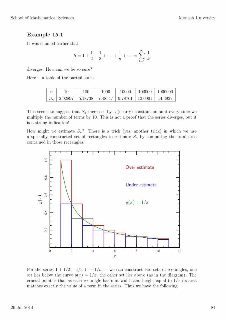
School of Mathematical Sciences Monash University
Example 15.1
It was claimed earlier that
S = 1 +1
2+
1
3+ · · ·+ 1
n+ · · · =
∞∑k=1
1
k
diverges. How can we be so sure?
Here is a table of the partial sums
n 10 100 1000 10000 100000 1000000
Sn 2.92897 5.18738 7.48547 9.78761 12.0901 14.3927
This seems to suggest that Sn increases by a (nearly) constant amount every time wemultiply the number of terms by 10. This is not a proof that the series diverges, but itis a strong indication!
How might we estimate Sn? There is a trick (yes, another trick) in which we usea specially constructed set of rectangles to estimate Sn by computing the total areacontained in those rectangles.
x
y(x)
Over estimate
Under estimate
y(x) = 1/x
0 2 4 6 8 10 12
0.2
0.4
0.6
0.8
1.0
For the series 1 + 1/2 + 1/3 + · · · 1/n · · · we can construct two sets of rectangles, oneset lies below the curve y(x) = 1/x, the other set lies above (as in the diagram). Thecrucial point is that as each rectangle has unit width and height equal to 1/x its areamatches exactly the value of a term in the series. Thus we have the following
26-Jul-2014 84

School of Mathematical Sciences Monash University
Below rectangles : B(n) = 1 + 12
+ 13
+ · · ·+ 1n−1
= Sn−1
Above rectangles : A(n) = 12
+ 13
+ · · ·+ 1n
= Sn − 1
Clearly we also have
B(n) <
∫ n
1
1
xdx < A(n)
but
∫ n
1
1
xdx = log(n)
and thus
Sn − 1 < log(n) < Sn−1
Now we can take the limit as n→∞,
limn→∞
Sn − 1 < limn→∞
log(n) < limn→∞
Sn−1
⇒ limn→∞
Sn − 1 <∞ < limn→∞
Sn−1
The left hand side of this inequality doesn’t tell us much but the right hand side showsclearly that limn→∞ Sn−1 is infinity. That is, the partial sums Sn do not converge andthe original series is divergent.
Note that the series
S = 1 +1
2+
1
3+ · · ·+ 1
n+ · · · =
∞∑k=1
1
k
is known as the Harmonic series.
15.1 The Integral Test
The previous example introduced a very powerful method for deciding if a series con-verges or diverges. The general approach is as follows.
Suppose we have an infinite series
S =∞∑k=0
ak
26-Jul-2014 85

School of Mathematical Sciences Monash University
and that the terms can be computed from a smooth function f(x) with ak = f(k) fork = 0, 1, 2 · · ·. Then
Sn − a0 <
∫ n
0
f(x) dx < Sn−1
We then take the limit as n→∞,
limn→∞
Sn − a0 <
∫ ∞0
f(x) dx < limn→∞
Sn−1
If we can evaluate the improper integral (or at least decide if it converges) then we willbe able to make a decision about the convergence of the infinite series.
I Convergence. If the improper integral converges then the infinite series con-verges.
I Divergence. If the improper integral diverges then so too does the infinite series.
Example 15.2
Show that
S =∞∑k=1
1
k2
is a convergent infinite series.
Example 15.3
For what values of p will the infinite series
S =∞∑k=1
kp
converge?
15.2 The Ratio test
This test first asks you to compute the limit
L = limn→∞
an+1
an
then we have
26-Jul-2014 86
School of Mathematical Sciences Monash University
Convergence : When L < 1
Divergence : When L > 1
Indeterminate : When L = 1
Example 15.4
Show, using the ratio test, that the geometric series S =∑∞
n=0 sn is convergent when
0 < s < 1.
Example 15.5
Show that
S =∞∑n=0
2n
n2 + 1
is a divergent series.
Example 15.6
What does the ratio test tell you about the Harmonic series?
26-Jul-2014 87
SCHOOL OF MATHEMATICAL SCIENCES
ENG1091
Mathematics for Engineering
16. Comparison test, alternating series.
School of Mathematical Sciences Monash University
16.1 Alternating series
So far we have only considered infinite series in which all of the terms were positive. Butthere are many infinite series in which the terms alternate from positive to negative.Here are two examples
S = 1− 1
2+
1
3− 1
4± · · · =
∞∑n=0
(−1)n
n+ 1
S ′ = 1− 1
3!+
1
5!− 1
7!± · · · =
∞∑n=0
(−1)n
(2n+ 1)!
These are known as alternating series. There is one very simple test for the convergenceof an alternating series.
If |an| → 0 as n→∞ then we have
Convergence : When |an+1| < |an| for all n > m
Divergence : In all other cases
where m is some (possibly large) number.
Example 16.1
Use the alternating series test to establish the convergence or otherwise of
S = 1− 1
2+
1
3− 1
4± · · · =
∞∑n=0
(−1)n
n+ 1
Example 16.2
Show that
S = 1− 1
3!+
1
5!− 1
7!± · · · =
∞∑n=0
(−1)n
(2n+ 1)!
is convergent.
Example 16.3
Draw a graph of Sn versus n for a typical alternating series. Study this graph andexplain why the infinite series is convergent when |an+1| < |an|.
26-Jul-2014 89

School of Mathematical Sciences Monash University
16.2 Non-positive infinite series
In general, an infinite series may contain any mix of positive an negative terms. Wehave looked at two classes, one where all the terms are positive and another where theterms alternate in sign.
What should we do with a general series? Given the general series
S =∞∑n=0
an
we construct a related series by taking the absolute value of each term,
S ′ =∞∑n=0
|an|
The mix of positive and negative terms in S actually works in favour of convergence forS. Thus if we can show that S ′ is convergent then we will also have shown that S isconvergent. On the other if we find that S ′ is divergent then we can not say anythingabout S.
Convergence : If S ′ converges, then so to does S
Indeterminate : In all other cases
This type of convergence is known as absolute convergence. If a series is not absolutelyconvergent we say that it is conditionally convergent.
Example 16.4
Show that −S ′ < S < S ′ and hence prove the previous assertion, that S convergeswhenever S ′ converges.
Example 16.5
Show that
S = 1− 1
22+
1
32− 1
42± · · · =
∞∑n=0
(−1)n
(n+ 1)2
converges.
16.3 Re-ordering an infinite series
There is one very useful consequence of absolute convergence.
If a series is absolutely convergent then you may re-order the terms in the infinite seriesin whatever way you like, the series will converge to the same value every time.
26-Jul-2014 90

School of Mathematical Sciences Monash University
Example 16.6
We know that the series
S = 1− 1
2+
1
3− 1
4± · · · =
∞∑n=0
(−1)n
n+ 1
is convergent. But suppose we grouped all the positive terms into one series and the allthe negative into another,
S = (1 +1
3+
1
5+
1
7+ · · · )
− (1
2+
1
4+
1
6+ · · · )
= S+ − S−
The two series S+ and S− can be shown (by comparison with the Harmonic series) todiverge. Thus we would have
S =∞−∞
and the right hand side is meaningless – it can be made to have any value you choose(by taking suitable limits for the partial sums for S+ and S−).
The moral is – do not re-order a conditionally convergent series!
26-Jul-2014 91

SCHOOL OF MATHEMATICAL SCIENCES
ENG1091
Mathematics for Engineering
17. Power series
School of Mathematical Sciences Monash University
17.1 Simple power series
Here are some typical examples of what are known as power series
f(x) = 1 + x+ x2 + x3 + · · ·+ xn + · · ·
g(x) = 1 + x+x2
2!+x3
3!+ · · ·+ xn
n!+ · · ·
h(x) = 1− x2
2!+x4
4!± · · ·+ (−1)n
x2n
(2n)!+ · · ·
Each power series is a function of one variable, in this case x and so they are also referredto as a power series in x.
We might like to ask
I For what values of x does the series converge?
I If the series converges, what value does it converge to?
The first question is a simple extension of the ideas we developed in the previous lectureswith the one exception that the convergence of the series may now depend upon thechoice of x.
The second question is generally much harder to answer. We will find, in the nextlecture, that it is easier to start with a known function and to then build a power seriesthat has the same values as the function (for values of x for which the power seriesconverges). By this method (Taylor series) we will see that the three power series aboveare representations of the functions f(x) = 1/(1− x), g(x) = ex and h(x) = cos(x).
17.2 The general power series
A power series in x around the point x = a is always of the form
a0 + a1(x− a) + a2(x− a)2 + · · ·+ an(x− a)n + · · · =∞∑n=0
an(x− a)n
The point x = a is often said to the be point around which the power series is based.
26-Jul-2014 93
School of Mathematical Sciences Monash University
17.3 Examples of Power Series
In a previous lecture it was claimed that
1
1− x = 1 + x+ x2 + x3 + · · ·+ xn + · · ·
ex = 1 + x+x2
2!+x3
3!+ · · ·+ xn
n!+ · · ·
cos(x) = 1− x2
2!+x4
4!± · · ·+ (−1)n
x2n
(2n)!+ · · ·
Our game today is to develop a method by which such power series can be constructed.
17.4 Maclaurin Series
Suppose we have a function f(x) and suppose we wish to re-express it as a power series.That is, we ask if it is possible to find the coefficients an such that
f(x) = a0 + a1x+ a2x2 + · · ·+ anx
n + · · · =∞∑n=0
anxn
is valid (for values of x for which the series converges).
Let’s just suppose that such an expansion is possible. How might we compute the an?There is a very neat trick which we will use. Note that if we evaluate both sides of theequation at x = 0 we get
f(0) = a0
That’s the first step. Now for a1 we first differentiate both sides of the equation for f(x),then put x = 0. The result is
df
dx
∣∣∣∣x=0
= a1
And we follow the same steps for all subsequent an. Here is summary of the first 4 steps.
f(x) = a0 + a1x+ a2x2 + a3x
3 + · · · ⇒ f(0) = a0
f ′(x) = a1 + 2a2x+ 3a3x2 + · · · ⇒ f ′(0) = a1
f ′′(x) = 2a2 + 6a3x+ · · · ⇒ f ′′(0) = 2a2
f ′′′(x) = 6a3 + · · · ⇒ f ′′′(0) = 6a3
26-Jul-2014 94

School of Mathematical Sciences Monash University
A power series developed in this way is known as a Maclaurin Series Here is a generalformula for computing a Maclaurin series.
Maclaurin Series
Let f(x) be an infinitely differentiable function at x = 0. Then
f(x) = a0 + a1x+ a2x2 + a3x
3 + · · ·+ anxn + · · ·
with
an =1
n!
dnf
dxn
∣∣∣∣x=0
Example 17.1
Compute the Maclaurin series for log(1 + x).
Example 17.2
Compute the Maclaurin series for sin(x).
17.5 Taylor Series
For a Maclaurin series we are required to compute the function and all its derivatives atx = 0. But many functions are singular at x = 0 so what should we do in such cases?
Simple – choose a different point around which to build the power series. Recall thatthe general power series for f(x) is of the form
f(x) = a0 + a1(x− a) + a2(x− a)2 + · · ·+ an(x− a)n + · · · =∞∑n=0
anxn
We can compute the an much as we did in the Maclaurin series with the one exceptionthat now we evaluate the function and its derivatives at x = a.
Taylor Series
Let f(x) be an infinitely differentiable function at x = a. Then
f(x) = a0 + a1(x− a) + a2(x− a)2 + · · ·+ an(x− a)n + · · ·
with
an =1
n!
dnf
dxn
∣∣∣∣x=a
26-Jul-2014 95

School of Mathematical Sciences Monash University
Example 17.3
Compute the Taylor series for log x around x = 1.
Example 17.4
Compute the Taylor series for sin(x) around x = π/2.
17.6 Uniqueness
Is it possible to have two different power series for the one function? That is, is itpossible to have
f(x) = a0 + a1(x− a) + a2(x− a)2 + · · ·+ an(x− a)n + · · ·
andf(x) = b0 + b1(x− a) + b2(x− a)2 + · · ·+ bn(x− a)n + · · ·
where the an and bn are different?
The simple answer is no. The coefficients of a Taylor series are unique.
What is the use of this fact? It means that regardless of how we happen to compute apower series we will always obtain the same results.
Example 17.5
Use the Taylor series
ex = 1 + x+x2
2!+x3
3!+ · · ·+ xn
n!+ · · ·
to compute a power series for e−x. Compare your result with the Taylor series for e−x.
Example 17.6
Show how the Taylor series for 1/(1 − x) can be used to obtain the Taylor series for1/(1− x)2.
If the proof of a theorem is not immediately apparent, it may be because you are tryingthe wrong approach. Below are some effective methods of proof that may aim you inthe right direction.
26-Jul-2014 96
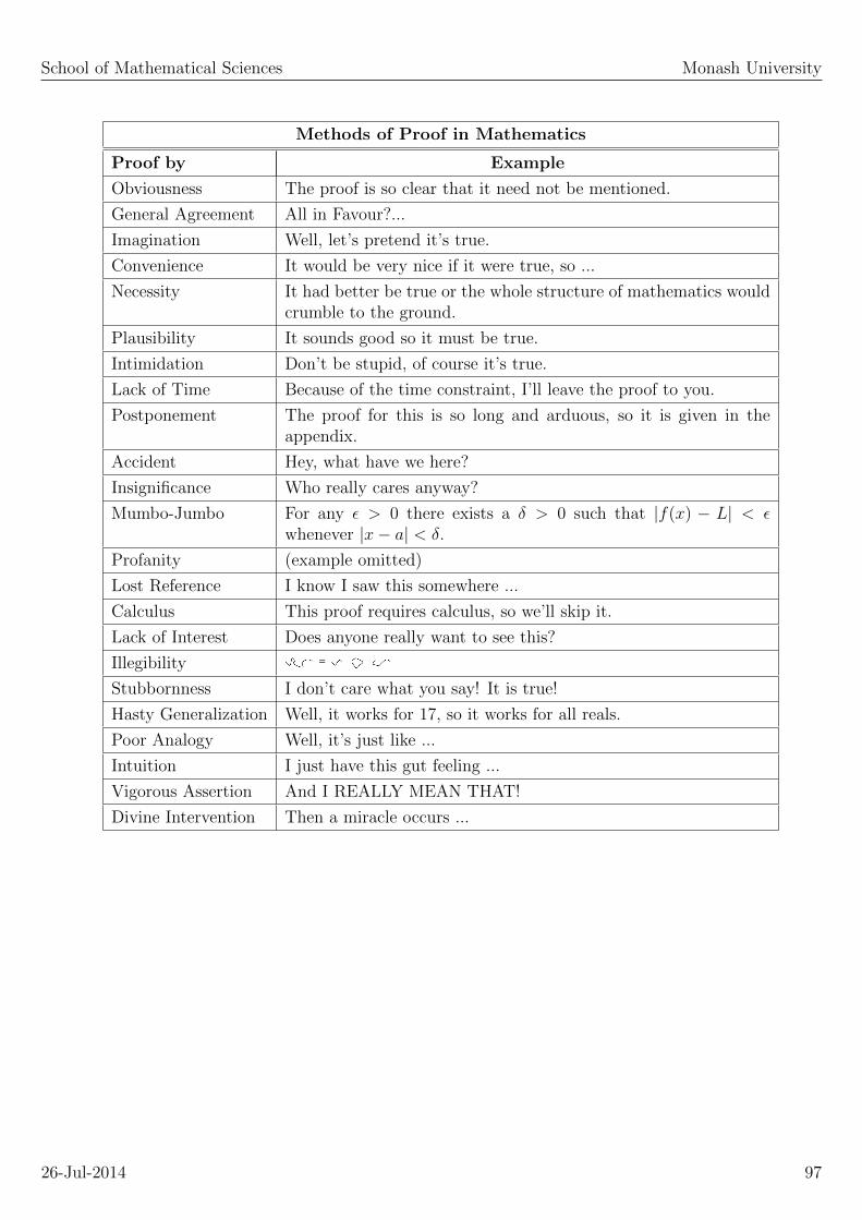
School of Mathematical Sciences Monash University
Methods of Proof in Mathematics
Proof by Example
Obviousness The proof is so clear that it need not be mentioned.
General Agreement All in Favour?...
Imagination Well, let’s pretend it’s true.
Convenience It would be very nice if it were true, so ...
Necessity It had better be true or the whole structure of mathematics wouldcrumble to the ground.
Plausibility It sounds good so it must be true.
Intimidation Don’t be stupid, of course it’s true.
Lack of Time Because of the time constraint, I’ll leave the proof to you.
Postponement The proof for this is so long and arduous, so it is given in theappendix.
Accident Hey, what have we here?
Insignificance Who really cares anyway?
Mumbo-Jumbo For any ε > 0 there exists a δ > 0 such that |f(x) − L| < εwhenever |x− a| < δ.
Profanity (example omitted)
Lost Reference I know I saw this somewhere ...
Calculus This proof requires calculus, so we’ll skip it.
Lack of Interest Does anyone really want to see this?
Illegibility
Stubbornness I don’t care what you say! It is true!
Hasty Generalization Well, it works for 17, so it works for all reals.
Poor Analogy Well, it’s just like ...
Intuition I just have this gut feeling ...
Vigorous Assertion And I REALLY MEAN THAT!
Divine Intervention Then a miracle occurs ...
26-Jul-2014 97

SCHOOL OF MATHEMATICAL SCIENCES
ENG1091
Mathematics for Engineering
18. Radius of convergence

School of Mathematical Sciences Monash University
18.1 Radius of convergence
If a series converges only for x in the interval |x−a| < R, then the radius of convergenceis defined to be R.
Note that it is possible to have R = 0 and even R =∞.
Example 18.1 : Finite radius of convergence
Consider the power series
f(x) = 1 + x+ x2 + x3 + · · ·+ xn + · · · =∞∑n=0
xn
This is the geometric series with common ratio x. We already know that this seriesconverges when |x| < 1 and thus its radius of convergence is 1.
Example 18.2
Use the ratio test to confirm the previous claim.
Example 18.3
Does the series converge for x = 1? Does it converge for x = −1? (These are minordot-the-i-cross-the-t type questions).
Example 18.4 : Infinite radius of convergence
Find the radius of convergence for the series
g(x) = 1 + x+x2
2!+x3
3!+ · · ·+ xn
n!+ · · · =
∞∑n=0
xn
n!
Example 18.5 : Zero radius of convergence
Find the the radius of convergence for the series
Q(x) = 1 + x+ 2!x2 + 3!x3 + · · ·+ n!xn + · · · =∞∑n=0
n!xn
18.2 Computing the Radius of Convergence
To compute the radius of convergence R for a power series of the form∑∞
0 an(x − a)n
you can take either of two approaches
26-Jul-2014 99

School of Mathematical Sciences Monash University
I Direct assault. Use the terms in the power series to define a new series bn =an(x − a)n. Then determine the convergence of
∑∞n=0 bn using any one of the
tests from previous lectures. Note that in this approach the bn must be treated asfunctions of x.
I Use a theorem. If you can compute limn→∞ |an+1|/|an| then this limit will be1/R. Note that this approach does not involve x.
Be careful not to confuse the two approaches!
Example 18.6
Find the radius of convergence for the series
f(x) =∑n=0
(−1)n+1 xn
n
18.3 Some theorems
Each of the following applies for x inside the interval of convergence.
I Absolute convergence. If the power series∑∞
n=0 |an(x − a)n| converges thenso to does
∑∞n=0 an(x− a)n.
I Term by term differentiation. A convergent power series may be differentiatedterm by term and it retains the same radius of convergence.
I Term by term integration. A convergent power series may be integrated termby term and it retains the same radius of convergence.
26-Jul-2014 100
SCHOOL OF MATHEMATICAL SCIENCES
ENG1091
Mathematics for Engineering
19. Function Approximation using Taylor Series
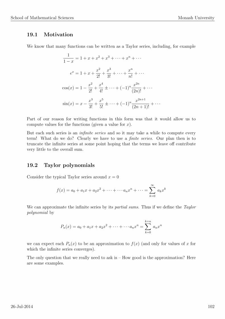
School of Mathematical Sciences Monash University
19.1 Motivation
We know that many functions can be written as a Taylor series, including, for example
1
1− x = 1 + x+ x2 + x3 + · · ·+ xn + · · ·
ex = 1 + x+x2
2!+x3
3!+ · · ·+ xn
n!+ · · ·
cos(x) = 1− x2
2!+x4
4!± · · ·+ (−1)n
x2n
(2n)!+ · · ·
sin(x) = x− x3
3!+x5
5!± · · ·+ (−1)n
x2n+1
(2n+ 1)!+ · · ·
Part of our reason for writing functions in this form was that it would allow us tocompute values for the functions (given a value for x).
But each such series is an infinite series and so it may take a while to compute everyterm! What do we do? Clearly we have to use a finite series. Our plan then is totruncate the infinite series at some point hoping that the terms we leave off contributevery little to the overall sum.
19.2 Taylor polynomials
Consider the typical Taylor series around x = 0
f(x) = a0 + a1x+ a2x2 + · · ·+ · · · anxn + · · · =
∞∑k=0
akxk
We can approximate the infinite series by its partial sums. Thus if we define the Taylorpolynomial by
Pn(x) = a0 + a1x+ a2x2 + · · ·+ · · · anxn =
k=n∑k=0
anxn
we can expect each Pn(x) to be an approximation to f(x) (and only for values of x forwhich the infinite series converges).
The only question that we really need to ask is – How good is the approximation? Hereare some examples.
26-Jul-2014 102

School of Mathematical Sciences Monash University
Example 19.1 : Taylor polynomials for cos(x)
The first four (distinct) Taylor polynomials for cos(x) are
P0(x) = 1
P2(x) = 1− x2
2!
P4(x) = 1− x2
2!+x4
4!
P6(x) = 1− x2
2!+x4
4!− x6
6!
and this is what they look like
x
y
cos(x)
P0(x)
P2(x)
P4(x)
P6(x)
−6 −4 −2 0 2 4 6
−1.0
−0.5
0.0
0.5
1.0
Example 19.2
Why were the other Taylor polynomials P1, P3, P5 not listed?
26-Jul-2014 103

School of Mathematical Sciences Monash University
Example 19.3
Using the above Taylor polynomials, estimate cos(0.1).
We observe that
I All of the approximations are close to cos(x) for x close to zero.
I The worst approximation is P0(x).
I The best approximation is P6(x)
We now ask two interesting questions
I How would we estimate cos(x) using a Taylor series for x = 12 given that P0(x), · · ·P6(x)appear to be very poor approximations near x = 12?
I Can we estimate the size of the error in approximations?
For the first question we have two lines of attack. Since we know that cos(x) is periodicwe can use
cos(12) = cos(12− 2π) = cos(12− 4π) = · · ·
As 12 − 4π is small we can expect that P3(12 − 4π) will be a good approximation tocos(12).
In general we do not have the luxury of having a periodic function and thus we need analternative method.
The second approach is to replace the current Taylor polynomials with a new set builtaround x = 4π. Thus we put a = 4π in a our general formula for the Taylor seriesleading to
P0(x) = 1
P2(x) = 1− (x− 4π)2
2!
P4(x) = 1− (x− 4π)2
2!+
(x− 4π)4
4!
P6(x) = 1− (x− 4π)2
2!+
(x− 4π)4
4!− (x− 4π)6
6!
26-Jul-2014 104
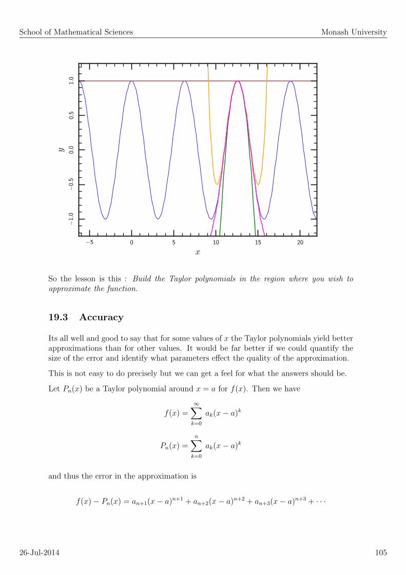
School of Mathematical Sciences Monash University
x
y
−5 0 5 10 15 20
−1.0
−0.5
0.0
0.5
1.0
So the lesson is this : Build the Taylor polynomials in the region where you wish toapproximate the function.
19.3 Accuracy
Its all well and good to say that for some values of x the Taylor polynomials yield betterapproximations than for other values. It would be far better if we could quantify thesize of the error and identify what parameters effect the quality of the approximation.
This is not easy to do precisely but we can get a feel for what the answers should be.
Let Pn(x) be a Taylor polynomial around x = a for f(x). Then we have
f(x) =∞∑k=0
ak(x− a)k
Pn(x) =n∑k=0
ak(x− a)k
and thus the error in the approximation is
f(x)− Pn(x) = an+1(x− a)n+1 + an+2(x− a)n+2 + an+3(x− a)n+3 + · · ·
26-Jul-2014 105

School of Mathematical Sciences Monash University
How do we estimate the right hand side? The usual trick is to assume that each eachterm is much smaller than its predecessor and thus the right hand side is dominated bythe first non-zero term.
Thus we often take
f(x)− Pn(x) ≈ an+1(x− a)n+1 =f (n+1)(a)
(n+ 1)!(x− a)n+1
where f (n+1)(a) is the n−th derivative of f(x) at x = a.
This is still a very loose mathematical argument. We have simply ignored all the remain-ing terms. A better estimate, but harder to justify, is given by the following theorem
Error bound for Taylor polynomials
If Pn(x) is the Taylor polynomial of degree n for the function f(x) in the interval|x− a| < R then the error En is bounded by
En = |f(x)− Pn(x)| < M
(n+ 1)!Rn+1
where M is the maximum value of |f (n+1)(x)| in the interval |x− a| < R.
The upshot of this is that we expect
I The error to be zero for polynomials of degree n or less, and
I The error, for a fixed x, to vary as (x− a)n+1 for varying choices of n.
Example 19.4 : Using the error estimate
Use the error bound to estimate how large the error might be in approximating sin(x)by P3(x) = x− x3/3! for x in the interval −1 < x < 1.
In this case we have R = 1, a = 0 and n = 3. For M we recall that every derivative ofsin is either ± sin or ± cos and thus we can take M = 1. Thus we have
E3 = | sin(x)− P3(x)| < M
(n+ 1)!Rn+1 =
1
4!14 =
1
24
Example 19.5
Use the error bound to estimate how large the error might be in approximating log(1+x)by P3(x) for x in the interval 0 < x < 2. Use a = 1 when computing P3.
26-Jul-2014 106

School of Mathematical Sciences Monash University
19.4 Using Taylor series to calculate limits
In your many and varied journeys in the world of mathematics you may have foundstatements like
1 = limx→0
sin(x)
x
and
1 = limx→1
log(x)
1− xand you may have been inclined to wonder how such statements can be proved (you dolike to know these things don’t you?). Our job in this section is develop a systematicmethod by which such hairy computations can be done with modest effort. But firsta clear warning – the following computations apply only to the troublesomeindeterminate form 0/0 (though it is possible to adapt our methods to cases such as∞/∞, we’ll come back to that later). If the calculation that troubles you is not of theform 0/0 then the following methods will give the wrong answer. Be very careful.
The functions in both of the above examples are of the form f(x)/g(x). Our road tofreedom (from the gloomy prison of 0/0) is to expand f(x) and g(x) as a Taylor seriesaround the point in question. The limits are then easy to apply. Let’s see this in actionfor the first example. Here we have
f(x) = sinx = x− 1
3!x3 +
1
5!x5 + · · ·
g(x) = x
In this case the Taylor series for g(x) was rather easy but that isn’t always the case.Thus we have
f(x)
g(x)=x− 1
3!x3 + 1
5!x5 + · · ·
x
= 1− 1
3!x2 +
1
5!x4 + · · ·
and this can be substituted into our expression for the limit,
limx→0
sin(x)
x= lim
x→01− 1
3!x2 +
1
5!x4 + · · ·
= 1
For our second example we must employ a Taylor series around x = 1. Thus we have
f(x) = log(x) = (x− 1)− 1
2(x− 1)2 +
1
3(x− 1)3 + · · ·
g(x) = 1− x = −(x− 1)1
26-Jul-2014 107

School of Mathematical Sciences Monash University
and so
limx→1
log(x)
1− x = limx→1
(x− 1)− 12(x− 1)2 + 1
3(x− 1)3 + · · ·
−(x− 1)
= limx→1−1 +
1
2(x− 1)− 1
3(x− 1)2 + · · ·
= −1
This is not all that hard, is it? Here is a slightly trickier example,
limx→0
1− cos(x)
sin(x2)=?
Once again we build the appropriate Taylor series (in this case around x = 0),
f(x) = 1− cos(x) =1
2!x2 − 1
4!x4 +
1
6!x6 + · · ·
g(x) = sin(x2) = x2 − 1
3!x6 +
1
5!x8 + · · ·
and so
limx→0
1− cos(x)
sin(x2)= lim
x→0
12!x2 − 1
4!x4 + 1
6!x6 + · · ·
x2 − 13!x6 + 1
5!x8 + · · ·
= limx→0
1
2!− 1
4!x2 +
1
6!x4 + · · ·
=1
2
By now the picture should be clear – a suitable pair of Taylor series can make shortwork of a troublesome 0/0 arising from expressions of the form f(x)/g(x).
19.5 l’Hopital’s rule.
Though the above method works very well it can be a bit tedious. You may have noticedthat our final answers depended only on the leading terms in the Taylor series and yet wecalculated the whole of the Taylor series. This looks like an un-necessary extra burden.Can we achieve the same result but with less effort? Most certainly, and here is how wedo it.
26-Jul-2014 108
School of Mathematical Sciences Monash University
l’Hopital’s rule for the form 0/0
If limx→a f(x) = 0 and limx→a g(x) = 0 then
limx→a
f(x)
g(x)= lim
x→a
f ′(x)
g′(x)
provided the limit exists. This rule can be applied recursively whenever the righthand side leads to 0/0.
Here is an outline of the proof. We start by writing out the Taylor series for f(x) andg(x) around x = a (while noting that f(a) = g(a) = 0)
f(x) = f ′(a)(x− a) +1
2!f ′′(a)(x− a)2 +
1
3!f ′′′(a)(x− a)3 + · · ·
g(x) = g′(a)(x− a) +1
2!g′′(a)(x− a)2 +
1
3!g′′′(a)(x− a)3 + · · ·
then
f(x)
g(x)=f ′(a)(x− a) + 1
2!f ′′(a)(x− a)2 + 1
3!f ′′′(a)(x− a)3 + · · ·
g′(a)(x− a) + 12!g′′(a)(x− a)2 + 1
3!g′′′(a)(x− a)3 + · · ·
=f ′(a) + 1
2!f ′′(a)(x− a) + 1
3!f ′′′(a)(x− a)2 + · · ·
g′(a) + 12!g′′(a)(x− a) + 1
3!g′′′(a)(x− a)2 + · · ·
If we assume that g′(a) 6= 0 then it follows that
limx→a
f(x)
g(x)=f ′(a)
g′(a)
This is not exactly l’Hopital’s rule but it gives you an idea of how it was constructed.With a little more care you can extend this argument to recover the full statement inl’Hopital’s rule (you need to consider cases where g′(a) = 0).
Example 19.6
Use l’Hoptal’s rule to verify the limits that we computed in the three detailed examplesgiven in the previous section.
We mentioned earlier that the tricks of this section could not only help us make sense ofexpressions like 0/0 but also for expressions like ∞/∞. Without going into the proofswe will just state the variation of l’Hopital’s rule for cases such as this – just do it! Yes,you can apply l’Hopital’s rule in the same manner as before. Here it is
26-Jul-2014 109
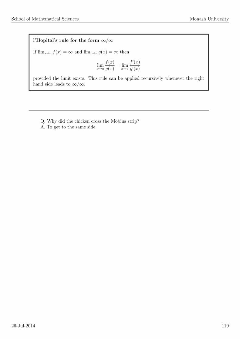
School of Mathematical Sciences Monash University
l’Hopital’s rule for the form ∞/∞
If limx→a f(x) =∞ and limx→a g(x) =∞ then
limx→a
f(x)
g(x)= lim
x→a
f ′(x)
g′(x)
provided the limit exists. This rule can be applied recursively whenever the righthand side leads to ∞/∞.
Q. Why did the chicken cross the Mobius strip?A. To get to the same side.
26-Jul-2014 110

SCHOOL OF MATHEMATICAL SCIENCES
ENG1091
Mathematics for Engineering
20. Remainder term for Taylor series.

School of Mathematical Sciences Monash University
20.1 Motivation
It must be admitted that our approach to developing a power series expansion for func-tions is somewhat cavalier. The weak spot in our analysis is that we have not given theinfinite series due respect. We saw earlier that it is easy to obtain non-sensical results ifwe make (rash) assumptions about the convergence of an infinite series. These are deli-cate areas and we must tread carefully. In this section we will use repeated integrationby parts to uncover each term in the power series. At each stage in the analysis we willbe working only with a finite series thus avoiding the delicate issues of convergence. Asan added bonus we will obtain, almost for free, an estimate of the error in using thefinite series as an approximation to the function. Excited? You should be.
20.2 Integration by parts and Taylor series
To get the ball rolling we will assume that we are given a function f(x) for which allof its derivatives exist in some interval centred on x = 0, say −R < x < R. Thatis, f, f ′, f ′′ etc. are finite for every x in −R < x < R. Now we start with the trivialequation
f(x) = f(0) +
∫ x
0
f ′(u) du
This is nothing more than the familiar rule for definite integrals (more correctly knownas the Fundamental Theorem of Integral Calculus). The integral on the right will nowbe manipulated by way of an integration by parts. To avoid confusion we will write theusual rule for integration by parts in the non-standard form∫
p′(u)q(u) du = p(u)q(u) +
∫−p(u)q′(u) du
For our case we will choose
p′(u) = −1 q(u) = f ′(u)
Now we need to compute p(u), the anti-derivate of p′(u) = −1 and q′(u) the derivativeof q(u). In integration by parts we would not normally include an integration constantwhen computing p(u) from p′(u) but on this occasion we will make a careful choice (thereason will become obvious soon). So we choose
p(u) = −(u− x) q′(u) = f ′′(u)
and this leads to
f(x) = f(0) +[−(u− x)f ′(u)
]u=x
u=0+
∫ x
0
−(u− x)f ′′(u) du
= f(0) + xf ′(0) +
∫ x
0
−(u− x)f ′′(u) du
26-Jul-2014 112
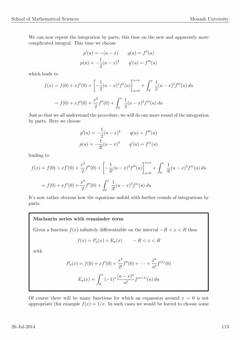
School of Mathematical Sciences Monash University
We can now repeat the integration by parts, this time on the new and apparently morecomplicated integral. This time we choose
p′(u) = −(u− x) q(u) = f ′′(u)
p(u) = −1
2(u− x)2 q′(u) = f ′′′(u)
which leads to
f(x) = f(0) + xf ′(0) +
[−1
2(u− x)2f ′′(u)
]u=x
u=0
+
∫ x
0
1
2(u− x)2f ′′′(u) du
= f(0) + xf ′(0) +x2
2f ′′(0) +
∫ x
0
1
2(u− x)2f ′′′(u) du
Just so that we all understand the procedure, we will do one more round of the integrationby parts. Here we choose
p′(u) = −1
2(u− x)2 q(u) = f ′′′(u)
p(u) = − 1
3!(u− x)3 q′(u) = f iv(u)
leading to
f(x) = f(0) + xf ′(0) +x2
2f ′′(0) +
[− 1
3!(u− x)3f ′′′(u)
]u=x
u=0
+
∫ x
0
1
3!(u− x)3f iv(u) du
= f(0) + xf ′(0) +x2
2f ′′(0) +
∫ x
0
1
3!(u− x)3f iv(u) du
It’s now rather obvious how the equations unfold with further rounds of integrations byparts.
Maclaurin series with remainder term
Given a function f(x) infinitely differentiable on the interval −R < x < R then
f(x) = Pn(x) + En(x) −R < x < R
with
Pn(x) = f(0) + xf ′(0) +x2
2!f ′′(0) + · · ·+ xn
n!f (n)(0)
En(x) =
∫ x
0
(−1)n(u− x)n
n!f (n+1)(u) du
Of course there will be many functions for which an expansion around x = 0 is notappropriate (for example f(x) = 1/x. In such cases we would be forced to choose some
26-Jul-2014 113

School of Mathematical Sciences Monash University
other point (say x = 1 for f(x) = 1/x) on which to build the power series. It is a simplematter to adapt the method just given for the Maclaurin series to this more generalcase. The result is as follows
Taylor series with remainder term
Given a function f(x) infinitely differentiable on the interval −R < x− a < R then
f(x) = Pn(x) + En(x) −R < x− a < R
with
Pn(x) = f(a) + (x− a)f ′(a) +(x− a)2
2!f ′′(a) + · · ·+ (x− a)n
n!f (n)(a)
En(x) =
∫ x
a
(−1)n(u− x)n
n!f (n+1)(u) du
The polynomial Pn(x) is commonly used as an approximation to f(x). The term En(x)is known as the remainder term. Later we shall see how we can use estimates of En(x)to not only provide a bound on the error incurred in using Pn(x) as an approximationto f(x) but also as another tool in deciding if the infinite series converges or diverges.
You might wonder if we have made any progress. We certainly have. No longer mustwe worry about the problems that come with working directly on an infinite series. Atevery stage in our analysis we have just three functions, f(x), a polynomial Pn(x) anda remainder term En(x). Each of these functions can be manipulated using any of thetools of algebra or calculus. This is a good place to be. From this solid foundation wecan carefully recover the infinite series by looking at En(x) in the limit as n→∞.
As an example, consider the function f(x) = ex which we will expand about the pointx = 0. Following the steps given above we would arrive at
ex = Pn(x) + En(x)
with
Pn(x) = 1 +x
1!+x2
2!+x3
3!+ · · ·+ xn
n!
En(x) =
∫ x
0
(−1)n(u− x)n
n!eu du
We can now ask (and answer) two interesting questions
I For a given n, how large might the error be in using Pn(x) as an approximation toex?
I For what values of x will the sequence Pn(x), n = 1, 2, 3, · · · converge?
26-Jul-2014 114

School of Mathematical Sciences Monash University
The answers can be found in a careful study of the remainder term En(x). Let us startwith the first question (how curious). Since ex = Pn(x) + En(x) we see that
|ex − Pn(x)| = |En(x)| =∫ x
0
(u− x)n
n!eu du
It is true that we could, after some effort, evaluate the right hand side to obtain theexact size of the error |ex−Pn(x)| but in most cases this is not easy to do (e.g.. try usingf(x) = ex
2). So the usual approach here is to make some simple assumptions about the
size of the terms in the integral so that we can obtain an equation of the form
|ex − Pn(x)| =∫ x
0
(u− x)n
n!eu du < Mn(x)
for some Mn(x). In this way Mn(x) serves an estimate for the error in using Pn(x) asan approximation for ex. Note that the particular form for Mn(x) will depend on theassumptions we make in simplifying the messy integral, different assumptions will leadto different functions Mn(x). Obviously our interest is finding a good estimate Mn(x).
Okay, enough of the game plan, let’s get back to our example. Since we know that themaximum for ex over the interval −R < x < R is eR we have∫ x
0
(u− x)n
n!eu du <
∫ x
0
(u− x)n
n!eR du
The right hand side is now a trivial integral and we obtain∫ x
0
(u− x)n
n!eu du < eR
xn+1
(n+ 1)!= Mn(x)
Thus we have
|ex − Pn(x)| < eRxn+1
(n+ 1)!
This gives us an answer to our first question. That is, the error in using Pn(x) as anapproximation to ex is no larger than eRxn+1/(n + 1)! for −R < x < R. It is alsogives us the tools needed to answer the second question. Notice that for any fixed x in−R < x < R we have
limn→∞
eRxn+1
(n+ 1)!= 0
In other words,ex = lim
n→∞Pn(x)
for −R < x < R. And as there is no restriction on R we see that we can allow R→∞and still guarantee convergence. In short, we have just shown that the infinite series
1 +x
1!+x2
2!+x3
3!+ · · ·+ xn
n!+ · · ·
converges to ex for any x and the radius of convergence is ∞.
26-Jul-2014 115

SCHOOL OF MATHEMATICAL SCIENCES
ENG1091
Mathematics for Engineering
21. Introduction to ODEs

School of Mathematical Sciences Monash University
21.1 Motivation
The mathematical description of the real world is most commonly expressed in equationsthat involve not just a function f(x) but also some of its derivatives. These equationsare known as ordinary differential equations (commonly abbreviated as ODEs). Hereare some typical examples.
I Newtonian gravity md2r(t)
dt2=−GMm
r2
I Population growthdN(t)
dt= −λN(t)
I Hanging chaind2y(x)
dx2= µ2y(x)
I Electrical currents LdI(t)
dt+RI(t) = E sin(ωt)
The challenge for us is to find the functions that are solutions to these equations. Theproblem is that there is no systematic way to solve an ODE; thus we are forced to lookat a range of strategies. This will be our game for the next few lectures. We will identifybroad classes of ODES and develop particular strategies for each class.
21.2 Definitions
Here are some terms commonly used in discussions on ODEs.
I Order The order of an ODE is the order of the highest derivative in theODE.
I Linear The ODE only contains terms linear in the function and its deriva-tives.
I Non-linear Any ODE that is not a linear ODE.
I Linear homogeneous A linear ODE that allows y = 0 as a solution.
I Dependent variable The solution of the ODE. Usually y.
I Independent variable The variable that the solution of the ODE dependson. Usually x or t.
I Boundary conditions A set of conditions that selects a unique solutionof the ODE. Essential for numerical work.
I Initial value problem An ODE with boundary conditions given at a sin-gle point. Usually found in time dependent prob-lems.
26-Jul-2014 117
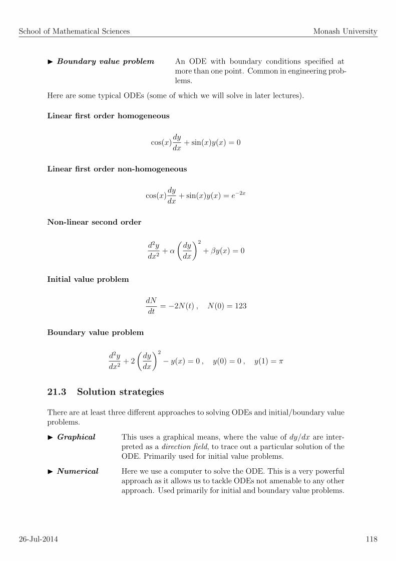
School of Mathematical Sciences Monash University
I Boundary value problem An ODE with boundary conditions specified atmore than one point. Common in engineering prob-lems.
Here are some typical ODEs (some of which we will solve in later lectures).
Linear first order homogeneous
cos(x)dy
dx+ sin(x)y(x) = 0
Linear first order non-homogeneous
cos(x)dy
dx+ sin(x)y(x) = e−2x
Non-linear second order
d2y
dx2+ α
(dy
dx
)2
+ βy(x) = 0
Initial value problem
dN
dt= −2N(t) , N(0) = 123
Boundary value problem
d2y
dx2+ 2
(dy
dx
)2
− y(x) = 0 , y(0) = 0 , y(1) = π
21.3 Solution strategies
There are at least three different approaches to solving ODEs and initial/boundary valueproblems.
I Graphical This uses a graphical means, where the value of dy/dx are inter-preted as a direction field, to trace out a particular solution of theODE. Primarily used for initial value problems.
I Numerical Here we use a computer to solve the ODE. This is a very powerfulapproach as it allows us to tackle ODEs not amenable to any otherapproach. Used primarily for initial and boundary value problems.
26-Jul-2014 118
School of Mathematical Sciences Monash University
I Analytical A full frontal assault with all the mathematical machinery we canmuster. This approach is essential if you need to find the fullgeneral solution of the ODE.
In this unit we will confine our attention to the last strategy, leaving numerical andgraphical methods for another day (no point over indulging on these nice treats).
So let’s get this show on the road with a simple example.
Example 21.1
Find all functions y(x) which obey
0 =dy
dx+ 2x
First we rewrite the ODE asdy
dx= −2x
then we integrate both sides with respect to x∫dy
dxdx = −2
∫x dx
But ∫dy
dxdx =
∫dy = y(x)− C
for any function y(x) and C is an arbitrary constant. Thus we have found
y(x) = C − x2
is a solution of the ODE for any choice of constant C. All solutions of the ODE mustbe of this form (for a suitable choice of C).
Example 21.2
Find all functions y(x) such that
0 =dy
dx+ 2xy
If we proceed as before we might arrive at∫dy
dxdx = −2
∫xy dx
The left hand side is easy to evaluate but the right hand side is problematic – we cannot easily compute its anti-derivative (we don’t yet know y(x)). So we need a differentapproach. This time we shuffle the y onto the left hand side,∫
1
y
dy
dxdx = −2
∫x dx
26-Jul-2014 119
School of Mathematical Sciences Monash University
But ∫1
y
dy
dxdx =
∫1
ydy = −C + log y
thus we findlog y = C − x2 ⇒ y(x) = Ae−x
2
We succeeded in this example because we were able to shuffle all x terms to one side ofthe equation and all y terms to the other. This is an example of a separable equation.We shall meet these equations again in later lectures.
In both of these example we found that one constant of integration popped up. Thismeans that we found not one solution but a whole family, each member having a differentvalue for C. This family of solutions is often called the general solution of the ODE.The role of boundary conditions (if given) is to allow a single member of the family tobe chosen.
21.4 General and particular solutions
Each time we take an anti-derivative, one constant of integration pops up. For a firstorder ODE we will need one anti-derivative and thus one constant of integration. But for,say, a third order equation, we will need to apply three anti-derivatives, each providingone constant of integration. What is the point of this discussion? It is the key to spottingwhen you have found all solutions of the ODE. This is what you need to know.
General solution of an ODE
If y(x) is a solution of an n−th order ODE and if y(x) contains n independentintegration constants then y(x) is the general solution of the ODE. Every solutionof the ODE will be found in this family.
Particular solution of an ODE
If y(x) is a solution of an n−th order ODE and if y(x) contains no free constants,then y(x) is a particular solution of the ODE.
Such solutions usually arise after the boundary conditions have been applied to thegeneral solution.
The great logician Betrand Russell once claimed that he could prove anythingif given that 1+1=1. So one day, some smarty-pants asked him, ”Ok. Provethat you’re the Pope.” He thought for a while and proclaimed, ”I am one.The Pope is one. Therefore, the Pope and I are one.”
26-Jul-2014 120

SCHOOL OF MATHEMATICAL SCIENCES
ENG1091
Mathematics for Engineering
22. Separable first order ODEs.
School of Mathematical Sciences Monash University
22.1 Separable equations
In an earlier example we solved
dy
dx=−xy
by first rearranging the equation so that y appeared only on the left hand side while xappeared only on the right hand side. Thus we found
∫y dy = −
∫x dx
and upon completing the integral for both sides we found
y2(x) = C − x2
This approach is known as separation of variables. It can only be applied to those ODEsthat allow us to shuffle the x and y terms onto separate sides of the ODE.
Separation of variables
If an ODE can be written in the form
dy
dx=f(x)
g(y)
then the ODE is said to be separable and its solution may be found from∫g(y) dy =
∫f(x) dx
Example 22.1
Show that the ODE
exdy
dx− 2y = 1
is separable. Hence solve the ODE.
26-Jul-2014 122

School of Mathematical Sciences Monash University
Example 22.2
Show that
sin(x)dy
dx+ y2 = cos(x)
is not separable.
Example 22.3
The number of bacteria in a colony is believed to grow according to the ODE
dN
dt= −2N
where N(t) is the number of bacteria at time t. Given that N = 20 initially, find N atlater times.
Example 22.4 : Newton’s law of cooling
This is a simple model of how the temperature of a warm body changes with time.
The rate of change of the body’s temperature is proportional to the difference betweenthe ambient and body temperatures. Write down a differential equation that representsthis model and then solve the ODE.
Example 22.5
Use the substitution u(x) = x2 + y(x) to reduce the non-separable ODE
du
dx= 3x− u
x
to a separable ODE. Hence obtain the general solution for u(x).
22.2 First order linear ODEs
This is a class of ODEs of the form
dy
dx+ P (x)y = Q(x)
where P (x) and Q(x) are known functions of x.
We will study two strategies to solve such ODEs.
26-Jul-2014 123

School of Mathematical Sciences Monash University
Example 22.6
Given
dy
dx+
1
xy = 0
find y(x).
For this ODE we have P (x) = 1/x and Q(x) = 0.
Solving this ODE is easy – it’s a separable ODE, thus we have
dy
y= −1
xdx
and after integrating both sides we find
y(x) =C
x
where C is a (modified) constant of integration.
Note that the above ODE has y(x) = 0 as a particular solution.
Whenever a linear ODE has y(x) = 0 as a solution we say that the ODE is homogeneous.
Example 22.7
Show that y(x) = x is a particular solution of
dy
dx+
1
xy = 2
We call it a particular solution because it does not contain an arbitrary constant ofintegration.
This ODE looks very much like the previous example with the one small change thatQ(x) = 2 rather than Q(x) = 0. We can expect that the general solution will be similarto the solution found in the previous example.
26-Jul-2014 124
School of Mathematical Sciences Monash University
Example 22.8
Show that
y(x) =C
x+ x
is the general solution of the ODE in the previous example.
Thus we have solved the ODE by a two step process, first by solving the homogeneousequation and second by finding any particular solution.
Strategy 1 for Linear 1st Order ODEs
Suppose that yh(x) is the general solution of the homogeneous equation
dyhdx
+ P (x)yh = 0
and suppose that yp(x) is any particular solution of
dy
dx+ P (x)y = Q(x)
Then the general solution of the previous ODE is
y(x) = yh(x) + yp(x)
Note, in some books yh(x) is written as yc(x) and is known as the complementary solu-tion.
Though this above procedure sounds easy we still have two problems,
I How do we compute the general solution of the homogeneous ODE?
I How do we obtain a particular solution?
22.2.1 Solving the homogeneous ODE
Setting Q(x) = 0 leads to
dy
dx+ P (x)y = 0
This is separable, thus we have
26-Jul-2014 125
School of Mathematical Sciences Monash University
dy
y= −P (x)dx
which we can integrate, with the result
y(x) = Ce−∫P (x) dx
Remember that this y(x) will be used as yh(x), the homogeneous solution of the non-homogeneous ODE.
Example 22.9
Verify the above solution for y(x)
22.2.2 Finding a particular solution
This usually involves some inspired guess work. The general idea is to look at Q(x)and then guess a class of functions for yp(x) that might be a solution of the ODE. Ifyou include few free parameters you may be able to find a particular solution – anyparticular solution will do.
Pi goes on and on and on ...And e is just as cursedI wonder: Which is largerWhen their digits are reversed?
26-Jul-2014 126

SCHOOL OF MATHEMATICAL SCIENCES
ENG1091
Mathematics for Engineering
23. The integrating factor.
School of Mathematical Sciences Monash University
23.1 The Integrating Factor
Example 23.1 : Easy
Use an inspired guess to find a particular solution of
dy
dx+ 3y = sin(x)
Example 23.2 : Harder
Use an inspired guess to find a particular solution of
dy
dx+ (1 + 3x)y = 3e−x
The main advantage of this method of inspired guessing (better known as the method ofundetermined coefficients) is that it is easy to apply. The main disadvantage is that it isnot systematic – it involves an element of guess work in finding the particular solution.
We need another, better and systematic strategy.
We begin by noticing that for any function I(x),
1
I
d(Iy)
dx=dy
dx+ y
1
I
dI
dx
The right hand side looks similar to the left hand side of our generic first order linearODE. We can make it exactly the same by choosing I(x) such that
P (x) =1
I
dI
dx
This is a separable ODE for I(x), with the particular solution
I(x) = e∫P (x) dx
So why our we doing this? Because once we know I(x) our original ODE may be re-written as
1
I
d(Iy)
dx= Q(x)
We can now integrate this,
26-Jul-2014 128

School of Mathematical Sciences Monash University
d(Iy)
dx= I(x)Q(x)
⇒∫
d(Iy)
dxdx =
∫I(x)Q(x) dx
⇒ I(x)y(x) =
∫I(x)Q(x) dx
⇒ y(x) =1
I(x)
∫I(x)Q(x) dx
The great advantage with this method is that it works every time! No guessing!
The function I(x) is known as the integrating factor.
Strategy 2 for Linear 1st Order ODEs
The general solution ofdy
dx+ P (x)y = Q(x)
is
y(x) =1
I(x)
∫I(x)Q(x) dx
where the integrating factor I(x) is given by
I(x) = e∫P (x) dx
Example 23.3
Find the general solution of
dy
dx+
1
xy = 2
Here we have P (x) = 1/x and Q(x) = 2.
26-Jul-2014 129

SCHOOL OF MATHEMATICAL SCIENCES
ENG1091
Mathematics for Engineering
24. Homogeneous Second order ODEs.
School of Mathematical Sciences Monash University
24.1 Second order linear ODEs
The most general second order linear ODE is
P (x)d2y
dx2+Q(x)
dy
dx+R(x)y = S(x)
Such a beast is not easy to solve. So we are going to make life easy for ourselves byassuming P (x), Q(x), R(x) and S(x) are constants. Thus we will be studying thereduced class of linear second order ODEs of the form
ad2y
dx2+ b
dy
dx+ cy = S(x)
where a, b, and c are constants.
No prizes for guessing that these are called constant coefficient equations.
We will consider two separate cases, the homogeneous equation where S(x) = 0 and thenon-homogeneous equation where S(x) 6= 0.
24.2 Homogeneous equations
Here we are trying to find all functions y(x) that are solutions of
ad2y
dx2+ b
dy
dx+ cy = 0
Let’s take a guess, let’s try
y(x) = eλx
We introduce the parameter λ as something to juggle in the hope that y(x) can be madeto be a solution of the ODE. First we need the derivatives,
y(x) = eλx ⇒ dy
dx= λeλx ⇒ d2y
dx2= λ2eλx
Then we substitute this into the ODE
0 = aλ2eλx + bλeλx + ceλx
⇒ 0 = (aλ2 + bλ+ c)eλx but eλx 6= 0
⇒ 0 = aλ2 + bλ+ c
26-Jul-2014 131

School of Mathematical Sciences Monash University
So we have a quadratic equation for λ, its two solutions are
λ1 =−b+
√b2 − 4ac
2aand λ2 =
−b−√b2 − 4ac
2a
Let’s assume for the moment that λ1 6= λ2 and that they are both real numbers.
What does this all mean? Simply that we have found two distinct solutions of the ODE,
y1(x) = eλ1x and y2(x) = eλ2x
Now we can use two of the properties of the ODE, one, that it is linear and two, that itis homogeneous, to declare that
y(x) = Ay1(x) +By2(x)
is also a solution of the ODE for any choice of constants A and B.
Example 24.1
Prove the previous claim, that y(x) is a solution of the linear homogeneous ODE.
And now comes the great moment of enlightenment – the y(x) just given contains twoarbitrary constants and as the general solution of a second order ODE must contain twoarbitrary constants we now realise that y(x) above is the general solution.
Example 24.2 : Real and distinct roots
Find the general solution of
d2y
dx2+dy
dx− 6y = 0
First we solve the quadratic
λ2 + λ− 6 = 0
for λ. This gives λ1 = 2 and λ2 = −3 and thus
y(x) = Ae2x +Be−3x
is the general solution.
The quadratic equation
26-Jul-2014 132
School of Mathematical Sciences Monash University
aλ2 + bλ+ c = 0
arising from the guess y(x) = eλx is known as the characteristic equation for the ODE.
We have already studied one case where the two roots are real and distinct. Now weshall look at some examples where the roots are neither real nor distinct.
Example 24.3 : Complex roots
Find the general solution of
d2y
dx2− 2
dy
dx+ 5y = 0
First we solve the quadratic
λ2 − 2λ+ 5 = 0
for λ. This gives λ1 = 1− 2i and λ2 = 1 + 2i. These are distinct but they are complex.That’s not a mistake just a venture into slightly unfamiliar territory. The full solutionis still given by
y(x) = Aeλ1x +Beλ2x = Ae(1−2i)x +Be(1+2i)x
This is a perfectly correct mathematical expression and it is the solution of the ODE.However, in cases where the solution of the ODE is to be used in a real-world problem,we would expect y(x) to be a real-valued function of the real variable x. In such caseswe must therefore have both A and B as complex numbers. This is getting a bit messyso it’s common practice to re-write the general solution as follows.
First recall that eiθ = cos θ + i sin θ and thus
e(1−2i)x = ex (cos(2x)− i sin(2x))
e(1+2i)x = ex (cos(2x) + i sin(2x))
and thus our general solution is also
y(x) = ex ((A+B) cos(2x) + (−iA+ iB) sin(2x))
Now A+ B and −iA+ iB are constants so let’s just replace them with a new A and anew B, that is we write
y(x) = ex (A cos(2x) +B sin(2x))
This the general solution of the ODE written in a form suitable for use with real numbers.
26-Jul-2014 133

School of Mathematical Sciences Monash University
Example 24.4 : Equal roots
Find the general solution of
d2y
dx2+ 2
dy
dx+ y = 0
This time we find just one root for λ,
λ1 = λ2 = −1
If we tried to declare that
y(x) = Aeλ1x +Beλ2x = Ae−x +Be−x
was the general solution we would be fooling ourselves. Why? Because in this case thetwo integration constants combine into one
y(x) = Ae−x +Be−x = (A+B)e−x = Ce−x
where C = A + B. We need two independent constants in order to have a generalsolution.
The trick in this case is this. Put
y(x) = (A+Bx)e−x
This does have two independent constants and you can show that this is a solution ofthe ODE for any choice of A and B. Thus it must also be the general solution.
The upshot of all of this is that when solving the general linear second order homogeneousODE we have three cases to consider, real and distinct roots, complex root and equalroots. The recipe to apply in each case is listed in the following table.
26-Jul-2014 134
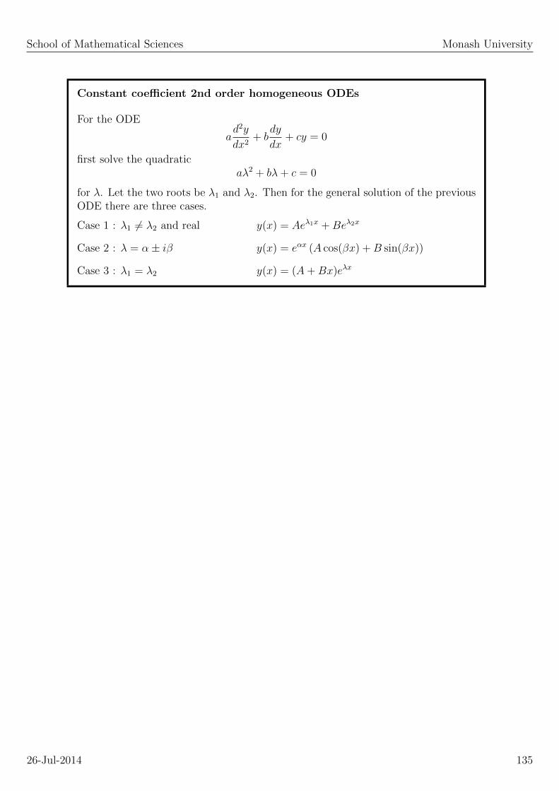
School of Mathematical Sciences Monash University
Constant coefficient 2nd order homogeneous ODEs
For the ODE
ad2y
dx2+ b
dy
dx+ cy = 0
first solve the quadraticaλ2 + bλ+ c = 0
for λ. Let the two roots be λ1 and λ2. Then for the general solution of the previousODE there are three cases.
Case 1 : λ1 6= λ2 and real y(x) = Aeλ1x +Beλ2x
Case 2 : λ = α± iβ y(x) = eαx (A cos(βx) +B sin(βx))
Case 3 : λ1 = λ2 y(x) = (A+Bx)eλx
26-Jul-2014 135

SCHOOL OF MATHEMATICAL SCIENCES
ENG1091
Mathematics for Engineering
25. Non-Homogeneous Second order ODEs.
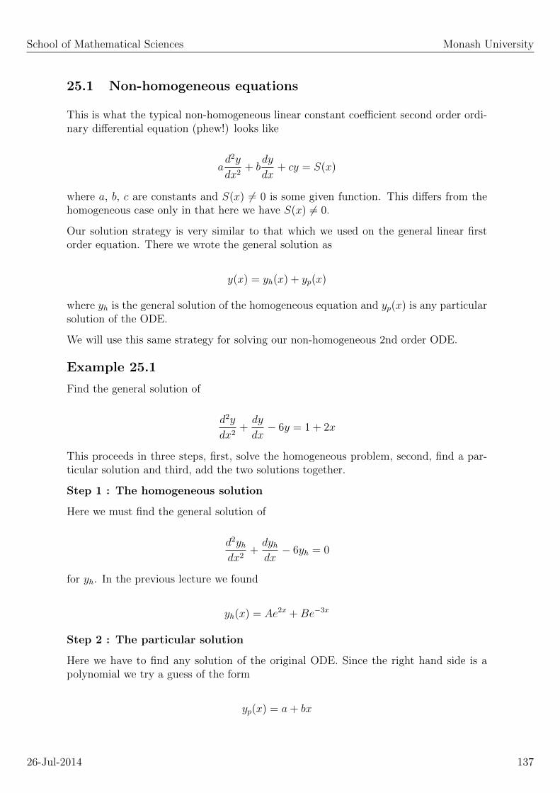
School of Mathematical Sciences Monash University
25.1 Non-homogeneous equations
This is what the typical non-homogeneous linear constant coefficient second order ordi-nary differential equation (phew!) looks like
ad2y
dx2+ b
dy
dx+ cy = S(x)
where a, b, c are constants and S(x) 6= 0 is some given function. This differs from thehomogeneous case only in that here we have S(x) 6= 0.
Our solution strategy is very similar to that which we used on the general linear firstorder equation. There we wrote the general solution as
y(x) = yh(x) + yp(x)
where yh is the general solution of the homogeneous equation and yp(x) is any particularsolution of the ODE.
We will use this same strategy for solving our non-homogeneous 2nd order ODE.
Example 25.1
Find the general solution of
d2y
dx2+dy
dx− 6y = 1 + 2x
This proceeds in three steps, first, solve the homogeneous problem, second, find a par-ticular solution and third, add the two solutions together.
Step 1 : The homogeneous solution
Here we must find the general solution of
d2yhdx2
+dyhdx− 6yh = 0
for yh. In the previous lecture we found
yh(x) = Ae2x +Be−3x
Step 2 : The particular solution
Here we have to find any solution of the original ODE. Since the right hand side is apolynomial we try a guess of the form
yp(x) = a+ bx
26-Jul-2014 137

School of Mathematical Sciences Monash University
where a and b are numbers (which we have to compute).
Substitute this into the left hand side of the ODE and we find
d2(a+ bx)
dx2+d(a+ bx)
dx− 6(a+ bx) = 1 + 2x
⇒ b− 6a− 6bx = 1 + 2x
This must be true for all x and so we must have
b− 6a = 1 and − 6b = 2
from which we get b = −1/3 and a = −2/9 and thus
yp(x) = −2
9− 1
3x
Note finding a particular solution be this guessing method is often called the method ofundetermined coefficients.
Step 3 : The general solution
This is the easy bit
y(x) = yh(x) + yp(x) = Ae2x +Be−3x − 2
9− 1
3x
Our job is done!
25.2 Undetermined coefficients
How do we choose a workable guess for the particular solution? Simply by inspectingthe terms in S(x), the right hand side of the ODE.
Here are some examples,
Guessing a particular solution
S(x) = (a+ bx+ cx2 + · · ·+ dxn)ekx
try yp(x) = (e+ fx+ gx2 + · · ·+ hxn)ekx
S(x) = (a sin(bx) + c cos(bx))ekx
try yp(x) = (c cos(bx) + f sin(bx))ekx
26-Jul-2014 138

School of Mathematical Sciences Monash University
Example 25.2
What guesses would you make for each of the following?
S(x) = 2 + 7x2
S(x) = (sin(2x))e3x
S(x) = 2x+ 3x3 + sin(4x)− 2xe−3x
25.3 Exceptions
Without exception there are always exceptions!
If S(x) contains terms that are solutions of the corresponding homogeneous equationthen in forming the guess for the particular solution you should multiply that term by x(and by x2 if the term corresponded to a repeated root of the characteristic equation).
Example 25.3
Find the general solution for
d2y
dx2+dy
dx− 6y = e2x
The homogeneous solution is
yh(x) = Ae2x +Be−3x
and thus we see that our right hand side contains a piece of the homogeneous solution.The guess for the particular solution would then be
yp(x) = (a+ bx)e2x
Now solve for a and b.
26-Jul-2014 139

SCHOOL OF MATHEMATICAL SCIENCES
ENG1091
Mathematics for Engineering
26. Coupled systems of ODEs
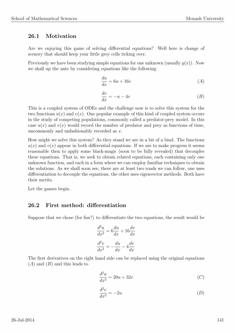
School of Mathematical Sciences Monash University
26.1 Motivation
Are we enjoying this game of solving differential equations? Well here is change ofscenery that should keep your little grey cells ticking over.
Previously we have been studying simple equations for one unknown (usually y(x)). Nowwe shall up the ante by considering equations like the following
du
dx= 6u+ 16v (A)
dv
dx= −u− 4v (B)
This is a coupled system of ODEs and the challenge now is to solve this system for thetwo functions u(x) and v(x). One popular example of this kind of coupled system occursin the study of competing populations, commonly called a predator-prey model. In thiscase u(x) and v(x) would record the number of predator and prey as functions of time,uncommonly and unfashionably recorded as x.
How might we solve this system? As they stand we are in a bit of a bind. The functionsu(x) and v(x) appear in both differential equations. If we are to make progress it seemsreasonable then to apply some black-magic (soon to be fully revealed) that decouplesthese equations. That is, we seek to obtain related equations, each containing only oneunknown function, and each in a form where we can employ familiar techniques to obtainthe solutions. As we shall soon see, there are at least two roads we can follow, one usesdifferentiation to decouple the equations, the other uses eigenvector methods. Both havetheir merits.
Let the games begin.
26.2 First method: differentiation
Suppose that we chose (for fun?) to differentiate the two equations, the result would be
d2u
dx2= 6
du
dx+ 16
dv
dx
d2v
dx2= −du
dx− 4
dv
dx
The first derivatives on the right hand side can be replaced using the original equations(A) and (B) and this leads to
d2u
dx2= 20u+ 32v (C)
d2v
dx2= −2u (D)
26-Jul-2014 141

School of Mathematical Sciences Monash University
It might seem that we are going backwards as we still have a coupled system and, quellehorror, we now have to contend with second derivatives. But there is light at the endof the tunnel. Look carefully at equations (A) and (C) and you will notice that thecombination (C) − 2(A) will eliminate v(x) from the right hand side. Likewise, thecombination (D)− 2(B) will eliminate u(x) from the right hand side. Here is what weget,
(C)− 2(A) ⇒ d2u
dx2− 2
du
dx− 8u = 0 (E)
(D)− 2(B) ⇒ d2v
dx2− 2
dv
dx− 8v = 0 (F )
Now we are happy, we have two equations with one unknown in each equation. Theseequations are easy to solve, namely
u(x) = Ae4x +Be−2x (G)
v(x) = Ce4x +De−2x (H)
We might be tempted to declare that this pair of equations define the full general solutionof the original ODEs. But we have a minor problem. In this so-called general solutionwe have four integration constants, A,B,C and D (not to be confused with the theequation labels). However, we started with just two first order ODEs and so we expectjust two integration constants, not four. Somehow we have to reduce the number ofconstants from four to two. Here is one way to do just that, substitute the solutions (G)and (H) back into the original ODE (A). This leads to
4Ae4x − 2Be−2x = 6(Ae4x +Be−2x
)+ 16
(Ce4x +De−2x
)= (6A+ 16C) e4x + (6B + 16D) e−2x
This must be true for all x, thus we can equate the coefficients of corresponding expo-nential terms leading to
4A = 6A+ 16C ⇒ A = −8C
−2B = 6B + 16D ⇒ B = −2D
Thus we have
u(x) = −8Ce4x − 2De−2x
v(x) = Ce4x +Dd−2x
Example 26.1
Use the solution for u(x) given by (G) to compute v(x) directly from equation (A).
26-Jul-2014 142
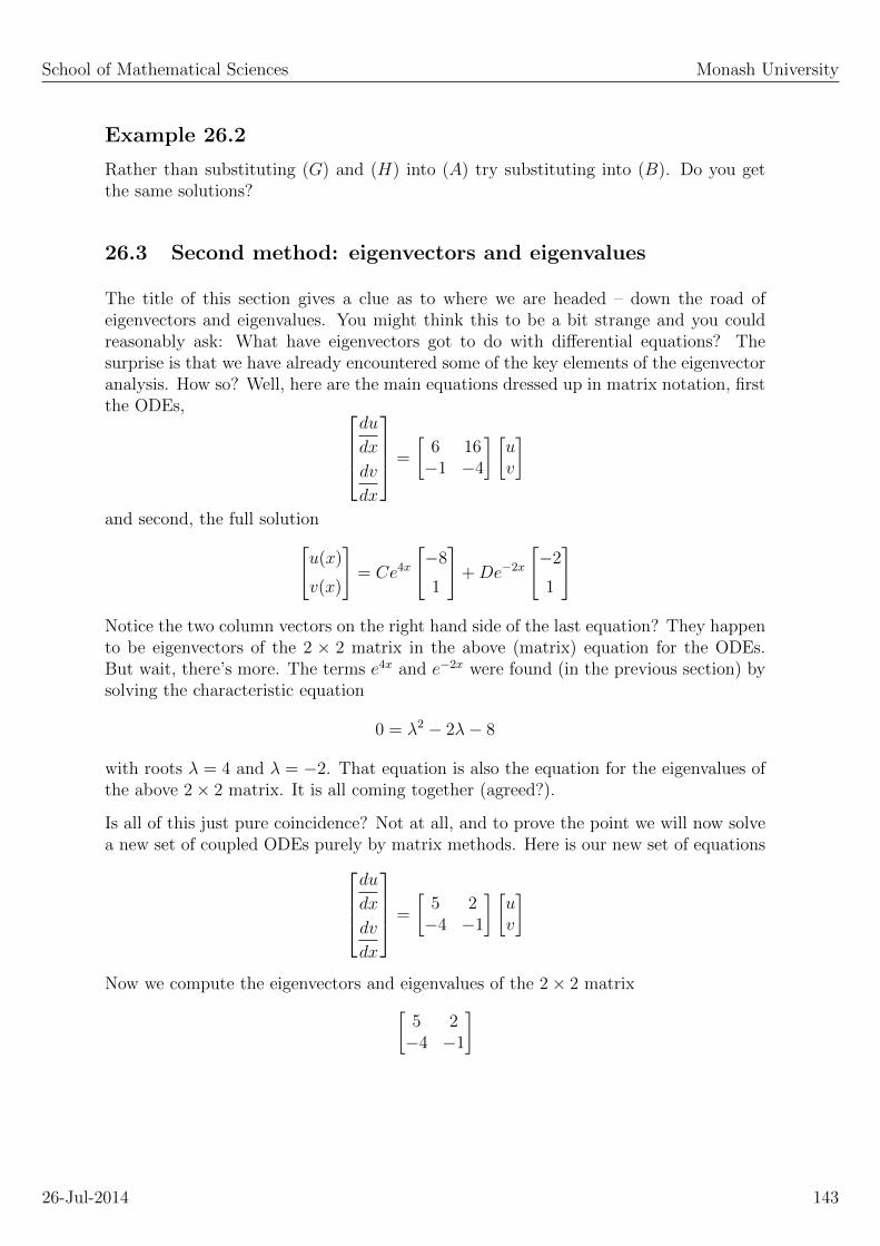
School of Mathematical Sciences Monash University
Example 26.2
Rather than substituting (G) and (H) into (A) try substituting into (B). Do you getthe same solutions?
26.3 Second method: eigenvectors and eigenvalues
The title of this section gives a clue as to where we are headed – down the road ofeigenvectors and eigenvalues. You might think this to be a bit strange and you couldreasonably ask: What have eigenvectors got to do with differential equations? Thesurprise is that we have already encountered some of the key elements of the eigenvectoranalysis. How so? Well, here are the main equations dressed up in matrix notation, firstthe ODEs,
du
dx
dv
dx
=
[6 16−1 −4
] [uv
]
and second, the full solution[u(x)
v(x)
]= Ce4x
[−8
1
]+De−2x
[−2
1
]
Notice the two column vectors on the right hand side of the last equation? They happento be eigenvectors of the 2 × 2 matrix in the above (matrix) equation for the ODEs.But wait, there’s more. The terms e4x and e−2x were found (in the previous section) bysolving the characteristic equation
0 = λ2 − 2λ− 8
with roots λ = 4 and λ = −2. That equation is also the equation for the eigenvalues ofthe above 2× 2 matrix. It is all coming together (agreed?).
Is all of this just pure coincidence? Not at all, and to prove the point we will now solvea new set of coupled ODEs purely by matrix methods. Here is our new set of equations
du
dx
dv
dx
=
[5 2−4 −1
] [uv
]
Now we compute the eigenvectors and eigenvalues of the 2× 2 matrix[5 2−4 −1
]
26-Jul-2014 143
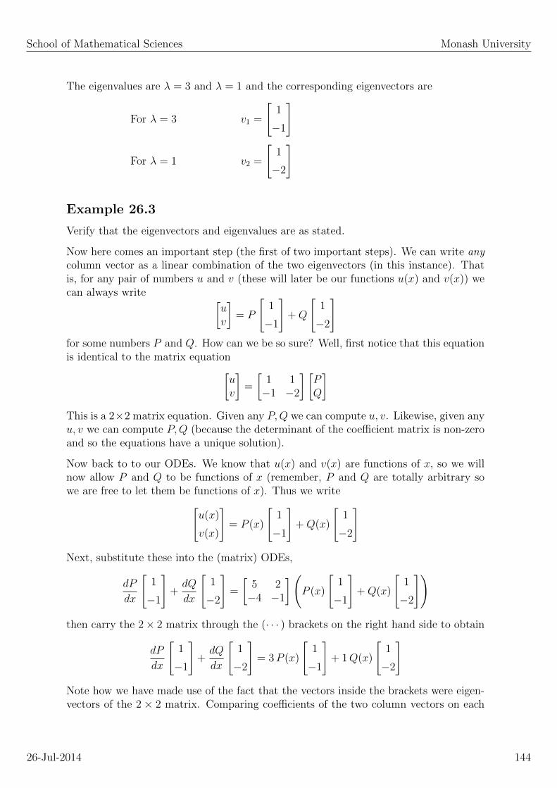
School of Mathematical Sciences Monash University
The eigenvalues are λ = 3 and λ = 1 and the corresponding eigenvectors are
For λ = 3 v1 =
[1
−1
]
For λ = 1 v2 =
[1
−2
]
Example 26.3
Verify that the eigenvectors and eigenvalues are as stated.
Now here comes an important step (the first of two important steps). We can write anycolumn vector as a linear combination of the two eigenvectors (in this instance). Thatis, for any pair of numbers u and v (these will later be our functions u(x) and v(x)) wecan always write [
uv
]= P
[1
−1
]+Q
[1
−2
]for some numbers P and Q. How can we be so sure? Well, first notice that this equationis identical to the matrix equation[
uv
]=
[1 1−1 −2
] [PQ
]This is a 2×2 matrix equation. Given any P,Q we can compute u, v. Likewise, given anyu, v we can compute P,Q (because the determinant of the coefficient matrix is non-zeroand so the equations have a unique solution).
Now back to to our ODEs. We know that u(x) and v(x) are functions of x, so we willnow allow P and Q to be functions of x (remember, P and Q are totally arbitrary sowe are free to let them be functions of x). Thus we write[
u(x)
v(x)
]= P (x)
[1
−1
]+Q(x)
[1
−2
]
Next, substitute these into the (matrix) ODEs,
dP
dx
[1
−1
]+dQ
dx
[1
−2
]=
[5 2−4 −1
](P (x)
[1
−1
]+Q(x)
[1
−2
])
then carry the 2× 2 matrix through the (· · · ) brackets on the right hand side to obtain
dP
dx
[1
−1
]+dQ
dx
[1
−2
]= 3P (x)
[1
−1
]+ 1Q(x)
[1
−2
]Note how we have made use of the fact that the vectors inside the brackets were eigen-vectors of the 2 × 2 matrix. Comparing coefficients of the two column vectors on each
26-Jul-2014 144

School of Mathematical Sciences Monash University
side of this equation (this is the second important step) gives us the following pair ofODEs
dP
dx= 3P and
dQ
dx= Q
This is a good. We now have two simple equations that are easily solved,
P (x) = Ae3x and Q(x) = Bex
where A and B are integration constants. And so finally we have our full solution of thecoupled ODEs [
u(x)
v(x)
]= Ae3x
[1
−1
]+Bex
[1
−2
]
Example 26.4
Look carefully at the last step leading to the ODEs for P (x) and Q(x). Why were weallowed to equate the coefficients of the two column vectors on each side of the equation?You might find it instructive to shuffle all the terms onto one side of the equals sign andthen write those equations as a 2× 2 matrix equation.
Example 26.5
Solve the above ODEs for u(x) and v(x) using the method given in the previous section.Verify that you get the same solution as given above (as you would expect).
It has been a long road. You might wonder why we would take such a long journey whena more direct method (as in the previous section using differentiation and elimination)is available. The answer is that it introduces you to a very powerful technique, the useof eigenvectors as a basis for a vector space, that can greatly simplify the algebraic com-plexity of many problems. This technique is used in many other areas of mathematics,most commonly in linear algebra, but also, as in this case, in solving differential equa-tions. It is also the corner stone of quantum mechanics, the wave function of a systemis a linear combination of eigenfunctions (a variation on the theme of eigenvectors).
26-Jul-2014 145

SCHOOL OF MATHEMATICAL SCIENCES
ENG1091
Mathematics for Engineering
27. Applications of Differential Equations

School of Mathematical Sciences Monash University
27.1 Applications of ODEs
In the past few lectures we studied, in detail, various techniques for solving a widevariety of differential equations. What we did not do is ask why we would want to solvethose equations in the first place. A simple (but rather weak) answer is that it is a niceintellectual challenge. A far better answer is that these ODEs arise naturally in thestudy of a vast array of physical problems, such as population dynamics, the spread ofinfectious diseases, the cooling of warm bodies, the swinging motion of a pendulum andthe motion of planets. In this lecture we shall look at some of these applications.
In each of the following examples we will not spend time computing the solution of theODE – this is left as an exercise for the (lucky) student!
27.2 Newton’s law of cooling
Newton’s law of cooling states that the rate of change of the temperature of a body isdirectly proportional to the temperature difference between the body and its surroundingenvironment. Let the temperature of the body be T and let Ta be that of the surroundingenvironment (the ambient temperature). Then Newton’s law of cooling is expressed inmathematical terms as
dT
dt= −k(T − Ta)
where k is some constant.
This is a simple non-homogeneous first order linear differential equation. Its generalsolution is
T (t) = Ta + Ae−kt
To apply this equation to a specific example we would need information that allows usto assign numerical values to the three parameters, Ta, k, and A.
Example 27.1 : A murder scene
We can use Newton’s law of cooling to estimate the time of death at a murder scene.Suppose the temperature of the body has been measured at 30 deg C. The normal bodytemperature is 37 deg C. So the question is – How long does it take for the body to coolfrom 37 deg C to 30 deg C? To answer this we need values for Ta, k, and A. Supposethe room temperature was 20 deg C and thus Ta = 20. For k we need to draw uponprevious experiments (how?). These show that a body left to cool in a 20 deg C roomwill drop from 37 deg C to 35 deg C in 2 hours. Substitute this into the above equationand we have
26-Jul-2014 147

School of Mathematical Sciences Monash University
T (0) = 37 = 20 + Ae0
T (2) = 35 = 20 + Ae−2k
Two equations in two unknowns, A and k. These are easy to solve, leading to
A = 17 and k =1
2loge
(17
15
)≈ 0.06258
ThusT (t) = 20 + 17e−0.06258t
Now for the time of the murder. Put T (t) = 30 and solve for t,
30 = 20 + 17e−0.06258t ⇒ t = − 1
0.06258loge
(10
17
)≈ 8.5
That is, the murder occurred about 8.5 hours earlier.
27.3 Pollution in swimming pools
Swimming pools should contain just two things – people and pure water. Yet all toooften the water is not pure. One way of cleaning the pool would be to pump in freshwater (at one point in the pool) while extracting the polluted water (at some otherpoint in the pool). Suppose we assume that the pool’s water remains thoroughly mixed(despite one entry and exit point) and that the volume of water remains constant. Canwe predict how the level of pollution changes with time?
Suppose at time t there is y(t) kgs of pollutant in the pool and that the volume of thepool is V litres. Suppose also that pure water is flowing in at the rate ρ litres/min and,since the volume remains constant, the outflow rate is also ρ litres/min.
Now we will set up a differential equation that describes how y(t) changes with time.
Consider a small time interval, from t to t + δt, where δt is a small number. In thatinterval ρδt litres of polluted water was extracted. How much pollutant did this carry?As the water is uniformly mixed we conclude that the density of the pollutant in theextracted water is the same as that in the pool. The density in the pool is y/V kg/Land thus the amount of pollutant carried away was (y/V )(ρδt). In the same small timeinterval no new pollutants were added to the pool. Thus any change in y(t) occurs solelyfrom the flow of pollutants out of the pool. We thus have
y(t+ δt)− y(t) = − yVρδt
26-Jul-2014 148

School of Mathematical Sciences Monash University
This can be reduced to a differential equation by dividing through by δt and then takingthe limit as δt→ 0. The result is
dy
dt= − ρ
Vy
The general solution is
y(t) = y(0)e−ρt/V
Example 27.2
Suppose the water pumps could empty the pool in one day. How long would it take tohalve the level of pollution?
27.4 Newtonian mechanics
The original application of ODEs was made by Newton (at the age of 22 in 1660) in thestudy of how things move. He formulated a set of laws, Newton’s laws of motion, oneof which states that the nett force acting on a body equals the mass of the body timesthe bodies acceleration.
Let F˜
be the force and let r˜
(t) be the position vector of the body. Then the body’svelocity and acceleration are defined by
v˜
(t) =dr
d̃t
a˜
(t) =dv
d̃t=d2 r˜dt2
Then Newton’s (second) law of motion may be written as
md2 r˜dt2 = F
˜If we know the force acting on the object then we can treat this as a second orderODE for the particle’s position r
˜(t). The usual method of solving this ODE is to write
r˜
(t) = x(t) i˜
+ y(t)j
˜+ z(t)k
˜and to re-write the above ODE as three separate ODEs,
one each for x(t), y(t) and z(t).
26-Jul-2014 149

School of Mathematical Sciences Monash University
md2x
dt2= Fx
md2y
dt2= Fy
md2z
dt2= Fz
where Fx, Fy, Fz are the components of the force in the directions of the (x, y, z) axes,F˜
= Fx i˜
+ Fy j
˜+ Fzk
˜.
Example 27.3 : Planetary motion
Newton also put forward a theory of gravitation – that there exists a universal force ofgravity, applicable to every lump of matter in the universe, that states that for any pairof objects the force felt by each object is given by
F =Gm1m2
r2
where m1 and m2 are the (gravitational) masses of the respective bodies, r is the distancebetween the two bodies and G is a constant (known as the Newtonian gravitationalconstant and by experiment is found to be 6.673×10⁻¹¹Nm2/kg2). The force is directedalong the line connecting the two objects.
Consider the motion of the Earth around the Sun. Each body will feel a force of gravityacting to pull the two together. Each body will move due to the action of the forceimposed upon it be the gravitational pull of its partner. However as the Sun is far moremassive than the Earth, the Sun will, to a very good approximation, remain stationarywhile the Earth goes about its business.
We can thus make the reasonable assumptions that
I The Sun does not move.
I The Sun is located at the origin of our coordinate system, x = y = z = 0
I The Earth orbits the Sun in the z = 0 plane.
Let r˜
(t) = x(t) i˜
+ y(t)j
˜be the position vector of the Earth. The force acting on the
Earth due to the gravitational pull of the Sun is then given by
F˜
= −GMm
r2r̂˜
26-Jul-2014 150
School of Mathematical Sciences Monash University
where r̂˜
is a unit vector parallel to r˜
, M is the mass of the Sun and m is the mass ofthe Earth. The minus sign shows that the force if pulling the Earth toward the Sun.The unit vector is easy to compute, r̂
˜= (x i
˜+ y j
˜)/r. Thus we have, finally,
md2x
dt2= −GMm
r2
x
r
md2y
dt2= −GMm
r2
y
r
This is a non-linear coupled system of ODEs – these are not easy to solve, so we resortto (more) simple approximations (in other Maths subjects!).
Example 27.4 : Simple Harmonic Motion
Many physical systems display an oscillatory behaviour, such as a swinging pendulumor a hanging weight attached to a spring. It seems reasonable then to expect the sinean cosine functions to appear in the description of these systems. So what type ofdifferential equation might we expect to see for such oscillatory systems? Simply thoseODEs that have the sine and cosine functions as typical solutions. We saw in previouslectures that the ODE
d2y
dt2= −k2y
has
y(t) = A cos(kt) +B sin(kt)
as its general solution. This the classic example of what is called simple harmonicmotion. Both the swinging pendulum and the weighted spring are described (actuallyapproximated) by the above simple harmonic equation.
26-Jul-2014 151

SCHOOL OF MATHEMATICAL SCIENCES
ENG1091
Mathematics for Engineering
28. Functions of Several Variables

School of Mathematical Sciences Monash University
28.1 Introduction
We are all familiar with simple functions such as y = sin(x). And we all know theanswers (don’t we?) to questions such as
1. What is its domain and the range ?
2. What does it look like as a plot in the xy-plane?
3. What is its derivative?
In this series of lectures we are going to up the ante by exploring similar questions forfunctions similar to z = cos(xy). This is just one example of what we call functionsof several variables. Though we will focus on functions that involve three variables(usually x, y and z) the lessons learnt here will be applicable to functions of any numberof variables.
28.2 Definition
A function f of two variables (x, y) is a single valued mapping of a subset of R2 into asubset of R.
What does this mean? Simply that for any allowed value of x and y we can compute asingle value for f(x, y). In a sense f is a process for converting pairs of numbers (x andy) into a single number f .
The notation R2 means all possible choices of x and y such as all points in the xy-plane.The symbol R denotes all real numbers (for example all points on the real line). Theuse of the word subset in the above definition is simply to remind us that functions havean allowed domain (i.e. a subset of R2) and a corresponding range (i.e. a subset of R).
Notice that we are restricting ourselves to real variables, that is the function’s value andits arguments (x, y) are all real numbers. This game gets very exciting and somewhattricky when we enter the world of complex numbers. Such adventures await you in lateryear mathematics (not surprisingly this area is known as Complex Analysis).
28.3 Notation
Here is a simple function of two variables
f(x, y) = sin(x+ y)
We can choose the domain to be R2 and then the range will be the closed set [−1,+1].Another common way of writing all of this is
f : (x, y) ∈ R2 7→ sin(x+ y) ∈ [−1, 1]
26-Jul-2014 153

School of Mathematical Sciences Monash University
This notation identifies the function as f , the domain as R2, the range as [−1, 1] andmost importantly the rule that (x, y) is mapped to sin(x + y). For this subject we willstick with the former notation.
You should also note that there is nothing sacred about the symbols x, y and f . Weare free to choose what ever symbols takes our fancy, for example we could concoct thefunction
w(u, v) = log(u− v)
Example 28.1
What would be a sensible choice of domain for the previous function?
28.4 Surfaces
A very common application of a function of two variables is to describe a surface in3-dimensional space. How so? you might ask. The idea is that we take the value of thefunction to describe the height of the surface above the xy-plane. If we use standardCartesian coordinates then such a surface could be described by the equation
z = f(x, y)
This surface has a height z units above each point (x, y) in the xy-plane.
The equation z = f(x, y) describes the surface explicitly as a height function over aplane and thus we say that the surface is given in explicit form.
A surface such as z = f(x, y) is also often called the graph of the function f .
Here are some simple examples. A very good exercise is to try to convince yourself thatthe following images are correct (i.e. that they do represent the given equation).
Note that in each of the following r is defined as r = +√
(x2 + y2).
26-Jul-2014 154

School of Mathematical Sciences Monash University
z = x2 + y2
1 = x2 + y2 − z2
z = cos (3πr) exp (−2r2)
26-Jul-2014 155
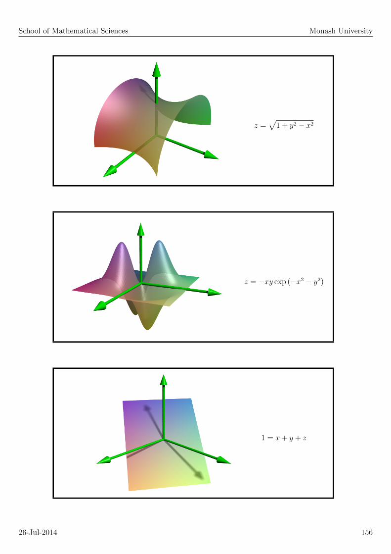
School of Mathematical Sciences Monash University
z =√
1 + y2 − x2
z = −xy exp (−x2 − y2)
1 = x+ y + z
26-Jul-2014 156

School of Mathematical Sciences Monash University
28.5 Alternative forms
We might ask are there any other ways in which we can describe a surface? We shouldbe clear that (in this subject) when we say surface we are talking about a 2-dimensionalsurface in our familiar 3-dimensional space. With that in mind, consider the equation
0 = g(x, y, z)
What do we make of this equation? Well, after some algebra we might be able tore-arrange the above equation into the familiar form
z = f(x, y)
for some function f . In this form we see that we have a surface, and thus the previousequation 0 = g(x, y, z) also describes a surface. When the surface is described by anequation of the form 0 = g(x, y, z) we say that the surface is given in implicit form.
Consider all of the points in R3 (i.e all possible (x, y, z) points). If we now introduce theequation 0 = g(x, y, z) we are forced to consider only those (x, y, z) values that satisfythis constraint. We could do so by, for example, arbitrarily choosing (x, y) and usingthe equation (in the form z = f(x, y) to compute z. Or we could choose say (y, z) anduse the equation 0 = g(x, y, z) to compute x. Which ever road we travel it is clear thatwe are free to choose just two of the (x, y, z) with the third constrained by the equation.
Now consider some simple surface and let’s suppose we are able to drape a sheet of graphpaper over the surface. We can use this graph paper to select individual points on thesurface (well as far as the graph paper covers the surface). Suppose we label the axesof the graph paper by the symbols u and v. Then each point on surface is described bya unique pair of values (u, v). This makes sense – we are dealing with a 2-dimensionalsurface and so we expect we would need 2 numbers ((u, v)) to describe each point on thesurface. The parameters (u, v) are often referred to as (local) coordinates on the surface.
How does this picture fit in with our previous description of a surface, as an equation ofthe form 0 = g(x, y, z)? Pick any point on the surface. This point will have both (x, y, z)and (u, v) coordinates. That means that we can describe the point in terms of either(u, v) or (x, y, z). As we move around the surface all of these coordinates will vary. Sogiven (u, v) we should be able to compute the corresponding (x, y, z) values. That is weshould be able to find functions P (u, v), Q(u, v) and R(u, v) such that
x = P (u, v) y = Q(u, v) z = R(u, v)
The above equations describe the surface in parametric form.
Example 28.2
Identify (i.e. describe) the surface given by the equations
x = 2u+ 3v + 1 y = u− 4v + 2 z = u+ 2v − 1
Hint : Try to combine the three equations into one equation involving x, y and z butnot u and v.
26-Jul-2014 157

School of Mathematical Sciences Monash University
Example 28.3
Describe the surface defined by the equations
x = 3 cos(φ) sin(θ) y = 4 sin(φ) sin(θ) z = 5 cos(θ)
for 0 < φ < 2π and 0 < θ < π
Example 28.4
How would your answer to the previous example change if the domain for θ was 0 < θ <π/2?
Equations for surfaces
A 2-dimensional surface in a 3-dimensional space may be described by any of thefollowing forms.
Explicit z = f(x, y)
Implicit 0 = g(x, y, z)
Parametric x = P (u, v), y = Q(u, v), z = R(u, v)
26-Jul-2014 158
SCHOOL OF MATHEMATICAL SCIENCES
ENG1091
Mathematics for Engineering
29. Partial derivatives

School of Mathematical Sciences Monash University
29.1 First derivatives
We all know and love the familiar definition of a derivative of a function of one variable,
df
dx= lim
∆x→0
f(x+ ∆x)− f(x)
∆x
The natural question to ask is : Is there similar rule for functions of more than onevariable? The answer is yes (surprised?) and we will develop the necessary formulas bya simple generalisation of the above definition.
Okay, let’s suppose we have a simple function, say f(x, y). Suppose for the moment thatwe pick a particular value of y, say y = 3. Then only x is allowed to vary and in effectwe now have a function of just one variable. Thus we can apply the above definition fora derivative which we write as
∂f
∂x= lim
∆x→0
f(x+ ∆x, y)− f(x, y)
∆x
Notice the use of the symbol ∂ rather than d. This is to remind us that in computingthis derivative all other variables are held constant (which in this instance is just y).
Of course we could play the same again but with x held constant, this leads to derivativein y,
∂f
∂y= lim
∆y→0
f(x, y + ∆y)− f(x, y)
∆y
Each of these derivatives, ∂f/∂x and ∂f/∂y are known as partial derivatives of f whilethe derivative of a function of one variable is often called an ordinary derivative.
You might think that we would now need to invent new rules for the (partial) derivativesof products, quotients and so on. But our definition of partial derivatives is built uponthe definition of an ordinary derivative of a function of one variable. Thus all thefamiliar rules carry over without modification. For example, the product rule for partialderivatives is
∂ (fg)
∂x= g
∂f
∂x+ f
∂g
∂x∂ (fg)
∂y= g
∂f
∂y+ f
∂g
∂y
Computing partial derivatives is no more complicated than computing ordinary deriva-tives.
26-Jul-2014 160

School of Mathematical Sciences Monash University
Example 29.1
If f(x, y) = sin(x) cos(y) then
∂f
∂x=
∂ sin(x) cos(y)
∂x
= cos(y)∂ sin(x)
∂x
= cos(y) cos(x)
Example 29.2
If g(x, y, z) = e−x2−y2−z2 then
∂g
∂z=
∂e−x2−y2−z2
∂z
= e−x2−y2−z2 ∂(−x2 − y2 − z2)
∂z
= −2ze−x2−y2−z2
29.2 Higher derivatives
The result of a partial derivative is another function of one or more variables. We are thusat liberty to take another derivative, generating yet another function. Clearly we canrepeat this any number of times (though possibly subject to some technical limitationsas noted below, see Exceptions).
Example 29.3
Let f(x, y) = sin(x) sin(y). Then we can define g(x, y) = ∂f/∂x and h(x, y) = ∂g/∂x.That is
g(x, y) =∂f
∂x=∂(
sin(x) sin(y))
∂x= cos(x) sin(y)
and
h(x, y) =∂g
∂x=∂(
cos(x) sin(y))
∂x= − sin(x) sin(y)
Example 29.4
Continuing from the previous example, compute ∂g/∂y.
26-Jul-2014 161

School of Mathematical Sciences Monash University
29.3 Notation
From the above example we see that h(x, y) was computed as follows
h(x, y) =∂g
∂x=∂
∂x
(∂f
∂x
)This is often written as
h(x, y) =∂2f
∂x2
Now consider the case where we compute h(x, y) by first taking a partial derivative inx then followed by a partial derivative in y, that is
h(x, y) =∂g
∂y=∂
∂y
(∂f
∂x
)and this is normally written as
h(x, y) =∂2f
∂y∂x
Note the order on the bottom line – you should read this from right to left. It tells youthat to take a partial derivative in x then a partial derivative in y.
It’s now a short leap to cases where we might take say 5 partial derivatives, such as
P (x, y) =∂5Q
∂x∂y∂y∂x∂x
Partial derivatives that involve one or more of the independent variables are known asmixed partial derivatives.
Example 29.5
Given f(x, y) = 3x2 + 2xy compute ∂2f/∂x∂y and ∂2f/∂y∂x. Notice anything?
Order of partial derivatives does not matter
If f is a twice-differentiable function, then the order in which its mixed partialderivatives are calculated does not matter. Each ordering will yield the same func-tion. For a function of two variables this means
∂2f
∂x∂y=
∂2f
∂y∂x
This is not immediately obvious but it can be proved (it’s a theorem!) and it is a veryuseful result.
26-Jul-2014 162

School of Mathematical Sciences Monash University
Example 29.6
Use the above theorem to show that
P (x, y) =∂5Q
∂x∂y∂y∂x∂x=
∂5Q
∂y∂y∂x∂x∂x=
∂5Q
∂x∂x∂x∂y∂y
This allows us to simplify our notation, all we need do is record how many of each typeof partial derivative are required, thus the above can be written as
P (x, y) =∂5Q
∂x3∂y2=
∂5Q
∂y2∂x3
29.4 Exceptions : when derivatives do not exist
In earlier lectures we noted that at the very least a function must be continuous if it isto have a meaningful derivative. When we take successive derivatives we may need torevisit the question of continuity for each new function that we create.
If a function fails to be continuous at some point then we most certainly can not takeits derivative at that point.
Example 29.7
Consider the function
f(x) =
{0 −∞ < x < 0
3x2 0 < x <∞
It is easy to see that something interesting might happen at x = 0. Its also not hard tosee that the function is continuous over its whole domain, and thus we can compute itsderivative everywhere, leading to
df(x)
dx=
{0 −∞ < x < 0
6x 0 < x <∞
This too is continuous and we thus attempt to compute its derivative,
d2f(x)
dx2=
{0 −∞ < x < 0
6 0 < x <∞
Now we notice that this second derivative is not continuous at x = 0. We thus can nottake any more derivatives at x = 0. Our chain of differentiation has come to an end.
We began with a continuous function f(x) and we were able to compute only its first twoderivatives over the domain x ∈ R. We say such that the function is twice differentiable
26-Jul-2014 163

School of Mathematical Sciences Monash University
over R. This is also often abbreviated by saying f is C2 over R. The symbol C reminds usthat we are talking about continuity and the superscript 2 tells us how many derivativeswe can apply before we encounter a non-continuous function. The clause ’over R’ justreminds us that the domain of the function is the set of real numbers (−∞,∞).
We should always keep in mind that a function may only posses a finite number ofderivatives before we encounter a discontinuity. The tell-tale signs to watch out for aresharp edges, holes or singularities in the graph of the function.
The Ten Commandments for Students of Mathematics
1. Thou shalt read Thy problem.
2. Whatsoever Thou doest to one side of ye equation, Do ye also to the other.
3. Thou must use Thy ”Common Sense”, else Thou wilt have flagpoles 9,000 metresin height, yea ... even fathers younger than sons.
4. Thou shalt ignore the teachings of false prophets to do work in Thy head.
5. When Thou knowest not, Thou shalt look it up, and if Thy search still elude Thee,Then Thou shalt ask the all-knowing teacher.
6. Thou shalt master each step before putting Thy heavy foot down on the next.
7. Thy correct answer does not prove that Thou hast worked Thy problem correctly.This argument convincest none, least of all, Thy teacher.
8. Thou shalt first see that Thou hast copied Thy problem correctly before bearingfalse witness that the answer book lieth.
9. Thou shalt look back even unto Thy youth and remember Thy arithmetic.
10. Thou shalt learn, speak, write, and listen correctly in the language of mathematics,and verily HD’s and D’s shall follow Thee even unto graduation.
26-Jul-2014 164
SCHOOL OF MATHEMATICAL SCIENCES
ENG1091
Mathematics for Engineering
30. Chain Rule, Gradient and Directional
derivatives

School of Mathematical Sciences Monash University
30.1 The Chain Rule
In a previous lecture we saw how could compute (partial) derivatives of functions ofseveral variables. The trick we employed was to reduce the number of independentvariables to just one (which we did by keeping all but one variable constant). There isanother way in which can achieve this reduction.
Consider a function of two variables f(x, y) and let’s suppose we are given a smoothcurve in the xy-plane. Each point on this curve can be characterised by its distancefrom some arbitrary starting point on the curve. In this way we can imagine that the(x, y) pairs on this curve are given as functions of one variable, let’s call it s. That is,our curve is described by the parametric equations
x = x(s), y = y(s)
for some functions x(s) and y(s). The values of the function f(x, y) on this curve aretherefore given by
f = f(x(s), y(s))
and this is just a function of one variable s. Thus we can compute its derivative df/ds.We will soon see that df/ds can be computed in terms of the partial derivatives.
Example 30.1
Given the curvex(s) = 2s, y(s) = 4s2 − 1 < s < 1
and the functionf(x, y) = 5x− 7y + 2
compute df/ds at s = 0.
Example 30.2
Show that for the curve x(s) = s, y(s) = 2 we get df/ds = ∂f/∂x.
Example 30.3
Show that for the curve x(s) = −1, y(s) = s we get df/ds = ∂f/∂y.
The last two examples show that df/ds is somehow tied to the partial derivatives of f .The exact link will be made clear in a short while (patience!).
What meaning can we assign to this number df/ds? It helps to imagine that we havedrawn a graph of f(x, y) (i.e. as a surface over the xy-plane).
Now draw the curve (x(s), y(s)) in the xy-plane and imagine walking along that curve,let’s call it C. At each point on C, f(s) is the height of the surface above the xy-plane.If you walk a short distance ∆s then the height might change by an amount ∆f . Therate at which the height changes with respect to the distance travelled is then ∆f/∆s.In the limit of infinitesimal distances we recover df/ds. Thus we can interpret df/ds as
26-Jul-2014 166

School of Mathematical Sciences Monash University
measuring the rate of change of f along the curve. This is exactly what we would haveexpected – after all derivatives measure rates-of-change.
The first example above showed how you could compute df/ds by first reducing f to anexplicit function of s. It was also hinted that it is also possible to evaluate df/ds usingpartial derivatives. Let’s now put some paint on the canvas!
Let’s go back to basics. The derivative df/ds could be calculated as
df
ds= lim
∆s→0
f(x(s+ ∆s), y(s+ ∆s))− f(x(s), y(s))
∆s
We will re-write this by adding and subtracting f(x(s), y(s+ ∆s)) just before the minussign. After a little rearranging we get
df
ds= lim
∆s→0
f(x(s+ ∆s), y(s+ ∆s))− f(x(s), y(s+ ∆s))
∆s
+ lim∆s→0
f(x(s), y(s+ ∆s))− f(x(s), y(s))
∆s
Now let’s look at the first limit. If we introduce ∆x = x(s + ∆s) − x(s) then we canwrite
lim∆s→0
f(x(s+ ∆s), y(s+ ∆s))− f(x(s), y(s+ ∆s))
∆s
= lim∆s→0
f(x(s+ ∆s), y(s+ ∆s))− f(x(s), y(s+ ∆s))
∆x
∆x
∆s
=∂f
∂x
dx
ds
We can write a similar equation for the second limit. Combining the two leads us to
df
ds=∂f
∂x
dx
ds+∂f
∂y
dy
ds
This is an extremely useful and important result. It is an example of what is known asthe chain rule for functions of several variables.
The Chain Rule
Let f = f(x, y) be a differentiable function. The chain rule for derivatives of falong a path x = x(s), y = y(s) is
df
ds=∂f
∂x
dx
ds+∂f
∂y
dy
ds
Now that we have a head of steam it’s rather easy to uncover an important extensionof the above result. Suppose the path was obtained by holding some other parameterconstant. That is, imagine that the path x = x(s), y = y(s) arose from some more
26-Jul-2014 167
School of Mathematical Sciences Monash University
complicated expressions such as x = x(s, t), y = y(s, t) with t held constant. How wouldour formula for the chain rule change? Not much other than we would have to keep inmind throughout that t is constant. We encountered this issue once before and that ledto partial rather than ordinary derivatives. Clearly the same change of notation applieshere, and thus we would write
∂f
∂s=∂f
∂x
∂x
∂s+∂f
∂y
∂y
∂s
as the first partial derivative of f with respect to s.
Let’s take stock. We are given a function of two variables f = f(x, y) and we are alsogiven two other functions, also of two variables, x = x(s, t), y = y(s, t). Then ∂f/∂s canbe calculated using the above chain rule.
Of course you could also compute ∂f/∂s directly by substituting x = x(s, t), y = y(s, t)into f(x, y) before taking the partial derivatives. Both approaches will give you exactlythe same answer.
Note that there is nothing special in the choice of symbols, x, y, s or t. You will oftenfind (u, v) used rather than (s, t).
Example 30.4
Given f = f(x, y) and x = 2s + 3t, y = s − 2t compute ∂f/∂t directly and by way ofthe chain rule.
The Chain Rule : Episode 2
Let f = f(x, y) be a differentiable function. If x = x(u, v), y = y(u, v) then
∂f
∂u=∂f
∂x
∂x
∂u+∂f
∂y
∂y
∂u
∂f
∂v=∂f
∂x
∂x
∂v+∂f
∂y
∂y
∂v
30.2 Gradient and Directional Derivative
Given any differentiable function of several variables we can compute each of its firstpartial derivatives. Let’s do something ‘out of the square’. We will assemble these partialderivatives as a vector which we will denote by ∇f . So for a function f(x, y) of twovariables we define
∇f =∂f
∂xi˜
+∂f
∂yj
˜The is known as the gradient of f and is often pronounced grad f.
26-Jul-2014 168

School of Mathematical Sciences Monash University
This may be pretty but what use is it? If we look back at the formula for the chain rulewe see that we can write it out as a vector dot-product,
df
ds=∂f
∂x
dx
ds+∂f
∂y
dy
ds
=
(∂f
∂xi˜
+∂f
∂yj
˜
)·(dx
dsi˜
+dy
dsj
˜
)= (∇f) ·
(dx
dsi˜
+dy
dsj
˜
)
What do we make of the vector on the far right of this equation? Its not hard to seethat it is a tangent vector to the curve (x(s), y(s)). And if we chose the parameter s tobe distance along the curve then we also see that its a unit vector.
Example 30.5
Prove the last pair of statements, that the vector is a tangent vector and that its a unitvector.
It is customary to denote the tangent vector by t˜
(some people prefer u˜
). With theabove definitions we can now re-write the equation for a directional derivative as follows
df
ds= t˜· ∇f
Isn’t that neat? The number that we calculate in this process df/ds is known as thedirectional derivative of f in the direction t
˜.
Yet another variation on the notation is to include the tangent vector as subscript on∇. Thus we also have
df
ds= ∇ t
˜f
Directional derivative
The directional derivative df/ds of a function f in the direction t˜
is given by
df
ds= t˜· ∇f = ∇ t
˜f
where the gradient ∇f is defined by
∇f =∂f
∂xi˜
+∂f
∂yj
˜and t
˜is a unit vector, t
˜· t˜
= 1.
26-Jul-2014 169

School of Mathematical Sciences Monash University
Example 30.6
Given f(x, y) = sin(x) cos(y) compute the directional derivative of f in the directiont˜
= ( i˜
+ j
˜)/√
2.
Example 30.7
Given ∇f = 2x i˜
+ 2y j
˜and x(s) = s cos(0.1), y(s) = s sin(0.1) compute df/ds at s = 1.
Example 30.8
Given f(x, y) = (xy)2 and the vector v˜
= 2 i˜
+ 7j
˜compute the directional derivative at
(1, 1). Hint : Is v˜
a unit vector?
We began this discussion by restricting a function of many variables to be a function ofone variable. We achieved this by choosing a path such as x = x(s), y = y(s). We mightask if the value of df/ds depends on the choice of the path? That is we could imaginemany different paths all sharing the one point, call it P , in common. Amongst thesedifferent paths might we get different answers for df/ds?
This is a very good question. To answer it let’s look at the directional derivative in theform
df
ds= t˜· ∇f
First we note that ∇f depends only on the values of (x, y) at P . It knows nothing aboutthe curves passing through P . That information is contained solely in the vector t
˜.
Thus if a family of curves passing through P share the same t˜
then we most certainlywill get the same value for df/ds for each member of that family. But what class ofcurves share the same t
˜at P? Clearly they are all tangent to each other at P . None of
the curves cross any other curve at P .
At this point we can dispense with the curves and retain just the tangent vector t˜
atP . All that we require to compute df/ds is the direction we wish to head in, t
˜, and the
gradient vector, ∇f , at P . Choose a different t˜
and you will get a different answer fordf/ds. In each case df/ds measures how rapidly f is changing the direction of t
˜.
A biologist, a statistician and a mathematician are on a photo-safari in africa. Theydrive out on the savannah in their jeep, stop and scout the horizon with their binoculars.
The biologist : Look! There’s a herd of zebras! And there, in the middle : A white zebra!It’s fantastic ! There are white zebra’s ! We’ll be famous !
The statistician : It’s not significant. We only know there’s one white zebra.
The mathematician : Actually, we only know there exists a zebra, which is white on oneside.
26-Jul-2014 170
SCHOOL OF MATHEMATICAL SCIENCES
ENG1091
Mathematics for Engineering
31. Tangent planes and linear approximations

School of Mathematical Sciences Monash University
31.1 Tangent planes
For functions of one variable we found that a tangent line provides a useful means ofapproximating the function. It is natural to ask how we might generalise this idea tofunctions of several variables.
Constructing a tangent line for a function of a single variable, f = f(x), is quite simple.Let’s just remind ourselves how we might do this. First we compute the function’s valuef and its gradient df/dx at some chosen point. We then construct a straight line withthese values at the chosen point.
Example 31.1
Construct the tangent line to f = sin(x) at x = π/4.
Notice that the tangent line is a linear function. Not surprisingly, for functions of severalvariables we will be constructing a linear function which shares particular properties withthe original function, in particular the function’s value and gradient at the chosen point.
Let’s be specific. Suppose we have a function f = f(x, y) of two variables and supposewe choose some point, say x = a, y = b. Let’s call this point P . At P we can evaluate fand all the first partial derivatives, ∂f/∂x and ∂f/∂y. Now we want to construct a newfunction, call it f̃ = f̃(x, y), that shares these some numbers at P . What conditions,apart from being linear, do we want to impose on f̃? Clearly we require
f̃p = fp ,
(∂f̃
∂x
)p
=
(∂f
∂x
)p
,
(∂f̃
∂y
)p
=
(∂f
∂y
)p
The subscript P is to remind us to impose these conditions at the point P .
As we want f̃ to be a linear function we could propose a function of the form
f̃(x, y) = C + Ax+By
We would need to carefully choose the numbers A,B,C so that we meet the aboveconditions. However, it is easier (and mathematically equivalent) to choose
f̃(x, y) = C + A(x− a) +B(y − b)
In this form we find
C = fp , A =
(∂f
∂x
)p
, B =
(∂f
∂y
)p
and thus we have
f̃(x, y) = fp + (x− a)
(∂f
∂x
)p
+ (y − b)(∂f
∂y
)p
This describes the tangent plane to the function f = f(x, y) at the point (a, b).
26-Jul-2014 172

School of Mathematical Sciences Monash University
Example 31.2
Prove that A,B,C are as stated.
In terms of ∇f we can write the tangent plane in the following form
f̃(r˜
) = fp + (r˜− r˜p) · (∇f)p
where r˜
= x i˜
+ y j
˜. This is a nice compact formula and it makes the transition to more
variables (x, y, z · · · ) trivial.
Example 31.3
Compute the tangent plane to the function f(x, y) = sin(x) sin(y) at (π/4, π/4).
The Tangent Plane
Let f = f(x, y) be a differentiable function. The tangent plane to f at the point Pis given by
f̃(x, y) = fp + (x− a)
(∂f
∂x
)p
+ (y − b)(∂f
∂y
)p
The tangent plane may be used to approximate f at points close to P .
31.2 Linear Approximations
We have done the hard work now it’s time to enjoy the fruits of our labour. We canuse the tangent plane as a way to estimate the original function in a region close to thechosen point. This is very similar to how we used a tangent line in approximations forfunctions of one variable.
Example 31.4
Use the result of the previous example to estimate sin(x) sin(y) at (5π/16, 5π/16).
Example 31.5
Would it make sense to use the same tangent plane as in the previous example to estimatef(5,−4)?
The bright and curious might now ask two very interesting questions, how large is theerror in the approximation and how can we build better approximations?
The answers to these questions takes us far beyond this subject but here is a very roughguide. Suppose you are estimating f at some point a distance ∆ away from P (that is,∆2 = (x − a)2 + (y − b)2). Then the error, |f(x, y) − f̃(x, y)| will be proportional to∆2. The proportionality factor will depend on the second derivatives of f (after all thisis what we left out in building the tangent plane). The upshot is that the error grows
26-Jul-2014 173

School of Mathematical Sciences Monash University
quickly as you move away from P but also, each time you halve the distance from P youwill reduce the error by a factor of four.
The answer to the second question, are there better approximations than a tangentplane, is most certainly yes. The key idea is to force the approximation to match higherderivatives of the original function. This leads to higher order polynomials in x and y.Such constructions are known as Taylor’s series in many variables. We will revisit thislater in the course but only in the context of functions of a single variable.
26-Jul-2014 174

SCHOOL OF MATHEMATICAL SCIENCES
ENG1091
Mathematics for Engineering
32. Maxima and minima

School of Mathematical Sciences Monash University
32.1 Maxima and minima
Suppose you run a commercial business and that by some means you have formulatedthe following formula for the profit of one of your lines of business
f = f(x, y) = 4− x2 − y2
Clearly the profit f depends on two variables x and y. Sound business practice suggestthat you would like to maximise your profits. In mathematical terms this means find thevalues of (x, y) such that f is a maximum. A simple plot of the graph of f shows us thatthe maximum occurs at (0, 0). For other functions we might not be so lucky and thuswe need some systematic way of computing the points (x, y) at which f is maximised.
You would have met (in previous years) similar problems for the case of a function ofone variable. And form that you may expect that for the present problem we will bemaking a statement about the derivatives of f in order that we have a maximum (i.e.that the derivatives should be zero). Let’s make this precise.
Let’s denote the (as yet unknown) point at which the function is a maximum by P .Now if we have a maximum at this point then moving in any direction from this pointshould see the function decrease. That is the directional derivative must be non-positivein every direction from P , thus we must have
df
ds= t˜· (∇f)p ≤ 0
for every choice of t˜
. Let’s be tricky. Let’s assume (for the moment) that (∇f)p 6= 0then we should be able to compute λ > 0 so that t
˜= λ (∇f)p is a unit vector. If you
now substitute this into the above you will find
λ (∇f)p · (∇f)p ≤ 0
Look carefully at the left hand side. Each term is positive (remember a˜· a˜
is the squaredlength of a vector a
˜) yet the right hand side is either zero or negative. Thus this equation
does not make sense and we have to reject our only assumption, that (∇f)p 6= 0.
We have thus found that if f is to have a maximum at P then we must have
0 = (∇f)p
This is a vector equation and thus each component of ∇f is zero at P , that is
0 =∂f
∂x, and 0 =
∂f
∂yat P
It is from these equations that we would compute the (x, y) coordinates of P .
Of course we could have posed the related question of finding the points at which afunction is minimised. The mathematics would be much the same save for a change inwords (maximum to minimum) and a corresponding change in ± signs. The end resultis the same, the gradient ∇f must vanish at P .
26-Jul-2014 176

School of Mathematical Sciences Monash University
Example 32.1
Find the points at which f = 4− x2 − y2 attains its maximum.
32.2 Local extrema
When we solve the equations0 = (∇f)p
we might get more than one point P . What do we make of these points? Some of themmight correspond to minimums while others might correspond to maximums of f . Doesthis exhaust all possibilities? No, there maybe some points which can not be classifiedas either a minima or a maxima of f . The three options are shown in the followinggraphs.
A typical local minimum
A typical local maximum
26-Jul-2014 177

School of Mathematical Sciences Monash University
A typical saddle point
A typical case might consist of any number of points like the above. It is for this reasonthat each point is referred to as a local maxima or a local minima.
32.3 Notation
Rather than continually having to qualify the point as corresponding to a minimum,maximum or a saddle point of f we commonly lump these into the one term localextrema.
Note when we talk of minima, maxima and extrema we are talking about the (x, y)points at which the function has a local minimum, maximum or extremum respectively.
32.4 Maxima, Minima or Saddle point?
You may recall that for a function of one variable, f = f(x), that its extrema could becharacterised simply be evaluating the sign of the second derivative. There is a similartest that we can apply for functions of two variables that is summarised in the followingbox. Note that this result is not examinable. It is included here to whet your appetitefor the exciting things that await in your later studies in maths (you will be doing morewon’t you?).
26-Jul-2014 178
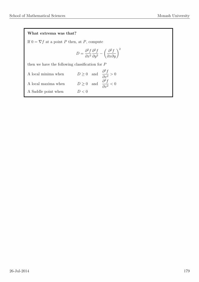
School of Mathematical Sciences Monash University
What extrema was that?
If 0 = ∇f at a point P then, at P , compute
D =∂2f
∂x2
∂2f
∂y2−(∂2f
∂x∂y
)2
then we have the following classification for P
A local minima when D ≥ 0 and∂2f
∂x2> 0
A local maxima when D ≥ 0 and∂2f
∂x2< 0
A Saddle point when D < 0
26-Jul-2014 179

School of Mathematical Sciences Monash University
Laborartory class exercises
Modern Engineering Mathematics, 4th ed.
Glyn James
Topic Exercises Questions
Vectors, Lines & Planes 4.2.8 17-20,23,254.2.10 31-344.3.3 52-55,59,60,62,63
Linear algebra 5.2.3 1,6,75.2.5 11,12,165.2.7 22
Matrices, Determinants & Matrix inverses 5.4.1 58,594.2.12 43-455.3.1 34,35,44
Eigenvalues & Eigenvectors 5.7.3 96,975.7.5 98-100,1025.7.8 105
Hyperbolic Functions 2.7.6 82,848.3.13 37,38
Integration by parts 8.8.4 105-107
Improper integrals 9.2.3 1
Sequences & Series 7.2.3 1,2,4,5,12,137.3.4 19,21,22,247.6.4 41,449.4.4 8-17
Introduction to ODEs 10.3.6 1,210.4.5 3-5
1st Order ODEs 10.5.4 11,13,15,1710.5.6 18,2010.5.11 31-35
2nd Order homogenous ODEs 10.9.2 55-61
2nd Order inhomogenous ODEs 10.9.4 62-65
Multivariable Calculus 9.6.4 37-469.6.6 47,48,50-559.6.8 56-649.6.10 65-72
Maxima & Minima 9.7.3 76,78
26-Jul-2014 180
School of Mathematical Sciences Monash University
Supplementary exercises
The questions on the following pages contain no new material not already covered bythe exercies in James. They are intended for students who want to practice their craftas far as they can (i.e., to do as many questions as possible, well done). These questionsmay also be helpful for students who do not have a copy of James to hand (but makeno mistake: James is an essential book for this unit, you should obtain a copy or leastknow where to find copies in the library).
Please note that the exercises provided by James for Improper Integrals is rather thin(just one question). So you are encouraged to complete the supplementary exercises onImproper Integrals. This will be sufficient study for questions of this kind should theyappear on the final exam.
26-Jul-2014 181
SCHOOL OF MATHEMATICAL SCIENCES
ENG1091
Mathematics for Engineering
Laboratory Class 1
Vectors, dot product, cross product
1. Find all the vectors whose tips and tails are among the three points with coordinates(2,−2, 3), (3, 2, 1) and (0,−1,−4).
2. Let v˜
= (3, 2,−2). How long is −2v˜
. Find a unit vector (a vector of length 1) in thedirection of v
˜.
3. For each pair of vectors given below, calculate the vector dot product and the angle θbetween the vectors.
(a) v˜
= (3, 2,−2) and w˜
= (1,−2,−1)
(b) v˜
= (0,−1, 4) and w˜
= (4, 2,−2)
(c) v˜
= (2, 0, 2) and w˜
= (−3,−2, 0)
4. Given the two vectors v˜
= (cos(θ), sin(θ), 0) and w˜
= (cos(φ), sin(φ), 0), use the dotproduct to derive the trigonometric identity
cos(θ − φ) = cos(θ) cos(φ) + sin(θ) sin(φ).
5. Use the dot product to determine which of the following two vectors are perpendicularto one another: u
˜= (3, 2,−2), v
˜= (1, 2,−2), w
˜= (2,−1, 2).
6. For each pair of vectors given below, calculate the vector cross product. Assuming thatthe vectors define a parallelogram, calculate the area of the parallelogram.
(a) v˜
= (3, 2,−2), w˜
= (1,−2,−1)
(b) v˜
= (0,−1, 4), w˜
= (4, 2,−2)
(c) v˜
= (2, 0, 2), w˜
= (−3,−2, 0)
7. Calculate the volume of the parallelepiped defined by the three vectors u˜
= (3, 2,−2), v˜
=(1, 2,−2), w
˜= (2,−1, 2).
8. Verify that v˜× w˜
= −w˜× v˜
.
School of Mathematical Sciences Monash University
Lines and planes
9. Consider the points (1, 2,−1) and (2, 0, 3).
(a) Find a vector equation of the line through these points in parametric form.
(b) Find the distance between this line and the point (1, 0, 1). (Hint: Use the para-metric form of the equation and the dot product.)
10. Find an equation of the plane that passes through the points (1, 2,−1), (2, 0,−1) and(−1,−1, 0).
11. Consider a plane defined by the equation 3x + 4y − z = 2 and a line defined by thefollowing vector equation (in parametric form)
x(t) = 2− 2t, y(t) = −1 + 3t, z(t) = −t.
(a) Find the point where the line intersects the plane. (Hint: Substitute the parametricform into the equation of the plane.)
(b) Find a normal vector to the plane.
(c) Find the angle at which the line intersects the plane. (Hint: Use the dot product.)
12. Find the distance between the parallel planes defined by the equations 2x−y+ 3z = −4and 2x− y + 3z = 24. (Hint: Use the cross product to construct a line normal to bothplanes, then use problem 11.)
13. Consider two planes defined by the equations 3x+ 4y − z = 2 and −2x+ y + 2z = 6.
(a) Find where the planes intersect the x, y and z axes.
(b) Find normal vectors for the planes.
(c) Find an equation of the line defined by the intersection of these planes. (Hint: Usethe normal vectors to define the direction of the line.)
(d) Find the angle between these two planes.
14. Find the minimum distance between the two lines defined by
x(t) = 1 + t, y(t) = 1− 3t, z(t) = −2 + 2t
andx(s) = 3s, y(s) = 1− 2s, z(s) = 2− s
(Hint: Use scalar projection as demonstrated in the lecture notes. Alternatively, definethe lines within parallel planes and then go back to problem 12.)
26-Jul-2014 183

SCHOOL OF MATHEMATICAL SCIENCES
ENG1091
Mathematics for Engineering
Laboratory Class 1 Solutions
Vectors, dot product, cross product
1. (0, 0, 0) ± (−1,−4, 2) ± (2,−1, 7) ± (3, 3, 5)
2. | − 2v˜| = 2
√17 , v
˜|v˜| = 1√
17(3, 2,−2)
3. (a) v˜· w˜
= 1, θ = arccos(
1√6·17
)≈ 1.4716 radians
(b) v˜· w˜
= −10, θ = arccos(−10√17·24
)≈ 2.0887 radians
(c) v˜· w˜
= −6, θ = arccos(−6√8·13
)≈ 2.1998 radians
4. v˜· w˜
= |v˜||w˜| cos(θ − φ) = 1 · 1 · cos(θ − φ) = cos(θ) cos(φ) + sin(θ) sin(φ)
5. u˜
and w˜
6. (a) v˜× w˜
= (−6, 1,−8) |v˜× w˜| =√
101
(b) v˜× w˜
= (−6, 16, 4) |v˜× w˜| = 2
√77
(c) v˜× w˜
= (4,−6,−4) |v˜× w˜| = 2
√17
7. (u˜× v˜
) · w˜
= 4
8. Yes, it is correct!
Lines and planes
9. (a) x(t) = 1 + t, y(t) = 2− 2t, z(t) = −1 + 4t
(b) 27
√14
10. 2x+ y + 7z = −3
11. (a) (2,−1, 0)
(b) (3, 4,−1)
(c) π2− arccos
(√91
26
)≈ 0.37567 radians

School of Mathematical Sciences Monash University
12.√
56
13. (a) (2/3, 0, 0), (0, 1/2, 0), (0, 0,−2) and (−3, 0, 0), (0, 6, 0), (0, 0, 3)
(b) (3, 4,−1) and (−2, 1, 2)
(c) x(t) = −2 + 9t, y(t) = 2− 4t, z(t) = 11t
(d) arccos(−2
39
√26)≈ 1.835 radians
14.√
3
26-Jul-2014 185
SCHOOL OF MATHEMATICAL SCIENCES
ENG1091
Mathematics for Engineering
Laboratory class 2
Row operations and linear systems
Solve each of the following system of equations using Gaussian elimination with back-substitution. Be sure to record the details of each row-operation (for example, as a noteon each row of the form (2)← 2(2)− 3(1).)
1.J + M = 75J − 4M = 0
2.x + y = 5
2x + 3y = 1
3.x + 2y − z = 6
2x + 5y − z = 13x + 3y − 3z = 4
4.x + 2y − z = 6x + 2y + 2z = 3
2x + 5y − z = 13
5.2x + 3y − z = 4x + y + 3z = 1x + 2y − z = 3
6. Repeat the last two questions, this time using Gaussian elimination (i.e. no back-substitution).
School of Mathematical Sciences Monash University
Under-determined systems
7. Using Gaussian elimination with back-substitution to find all possible solutions for thefollowing system of equations
x + 2y − z = 6x + 3y = 7
2x + 5y − z = 13
8. Find all possible solutions for the system (sic) of equations
x + 2y − z = 6
(Hint : You have one equation but three unknowns. You will need to introduce two freeparameters).
Matrices
9. Evaluate each of the following matrix operations
2
[1 11 −4
]−[
2 −13 1
],
[1 11 −4
] [2 −13 1
],
[1 1 31 −4 2
] 2 −13 11 2
10. Rewrite the equations for questions 1,2 and 3 in matrix form. Hence write down the
coefficient and augmented matrices for questions 1,2 and 3.
11. Repeat the row-operations part of questions 4 and 5 using matrix notation (should beeasy).
Matrix inverses
12. Compute the inverse A−1 of the following matrices
A =
[1 11 −4
]A =
2 3 −11 1 31 2 −1
Verify that A−1A = I and AA−1 = I.
13. Use the result of the previous question to solve the system of equations in questions 1and 5.
26-Jul-2014 187

School of Mathematical Sciences Monash University
Matrix determinants
14. Compute the determinant for the coefficient matrices in questions 7 and 8. What doyou observe?
15. For the matrix
A =
2 3 −11 1 31 2 −1
compute the determinant twice, first by expanding about the top row and second byexpanding about the second column.
16. Given
A =
[1 11 −4
], B =
[2 −13 1
]compute det(A), det(B) and det(AB). Verify that det(AB) = det(A) det(B).
26-Jul-2014 188
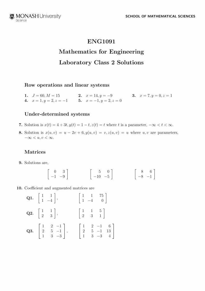
SCHOOL OF MATHEMATICAL SCIENCES
ENG1091
Mathematics for Engineering
Laboratory Class 2 Solutions
Row operations and linear systems
1. J = 60,M = 15 2. x = 14, y = −9 3. x = 7, y = 0, z = 14. x = 1, y = 2, z = −1 5. x = −1, y = 2, z = 0
Under-determined systems
7. Solution is x(t) = 4 + 3t, y(t) = 1− t, z(t) = t where t is a parameter, −∞ < t <∞.
8. Solution is x(u, v) = u − 2v + 6, y(u, v) = v, z(u, v) = u where u, v are parameters,−∞ < u, v <∞.
Matrices
9. Solutions are,[0 3−1 −9
] [5 0
−10 −5
] [8 6−8 −1
]
10. Coefficient and augmented matrices are
Q1.
[1 11 −4
],
[1 1 751 −4 0
]
Q2.
[1 12 3
],
[1 1 52 3 1
]
Q3.
1 2 −12 5 −11 3 −3
, 1 2 −1 6
2 5 −1 131 3 −3 4
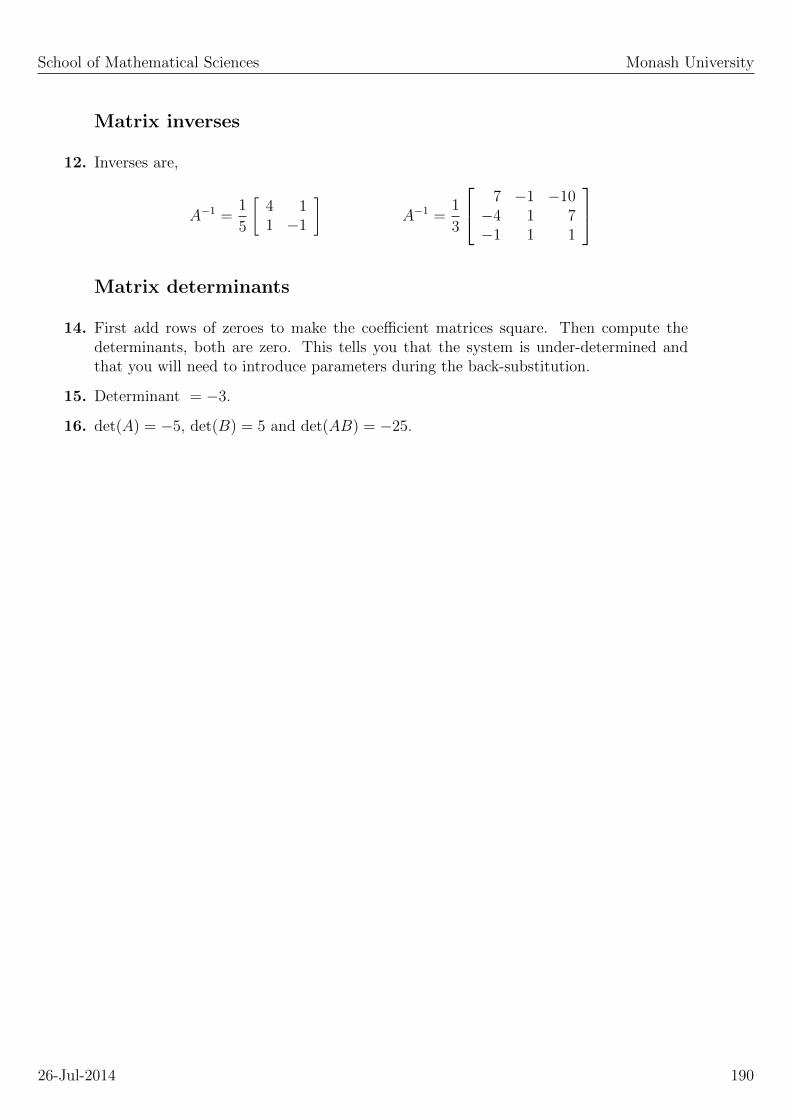
School of Mathematical Sciences Monash University
Matrix inverses
12. Inverses are,
A−1 =1
5
[4 11 −1
]A−1 =
1
3
7 −1 −10−4 1 7−1 1 1
Matrix determinants
14. First add rows of zeroes to make the coefficient matrices square. Then compute thedeterminants, both are zero. This tells you that the system is under-determined andthat you will need to introduce parameters during the back-substitution.
15. Determinant = −3.
16. det(A) = −5, det(B) = 5 and det(AB) = −25.
26-Jul-2014 190
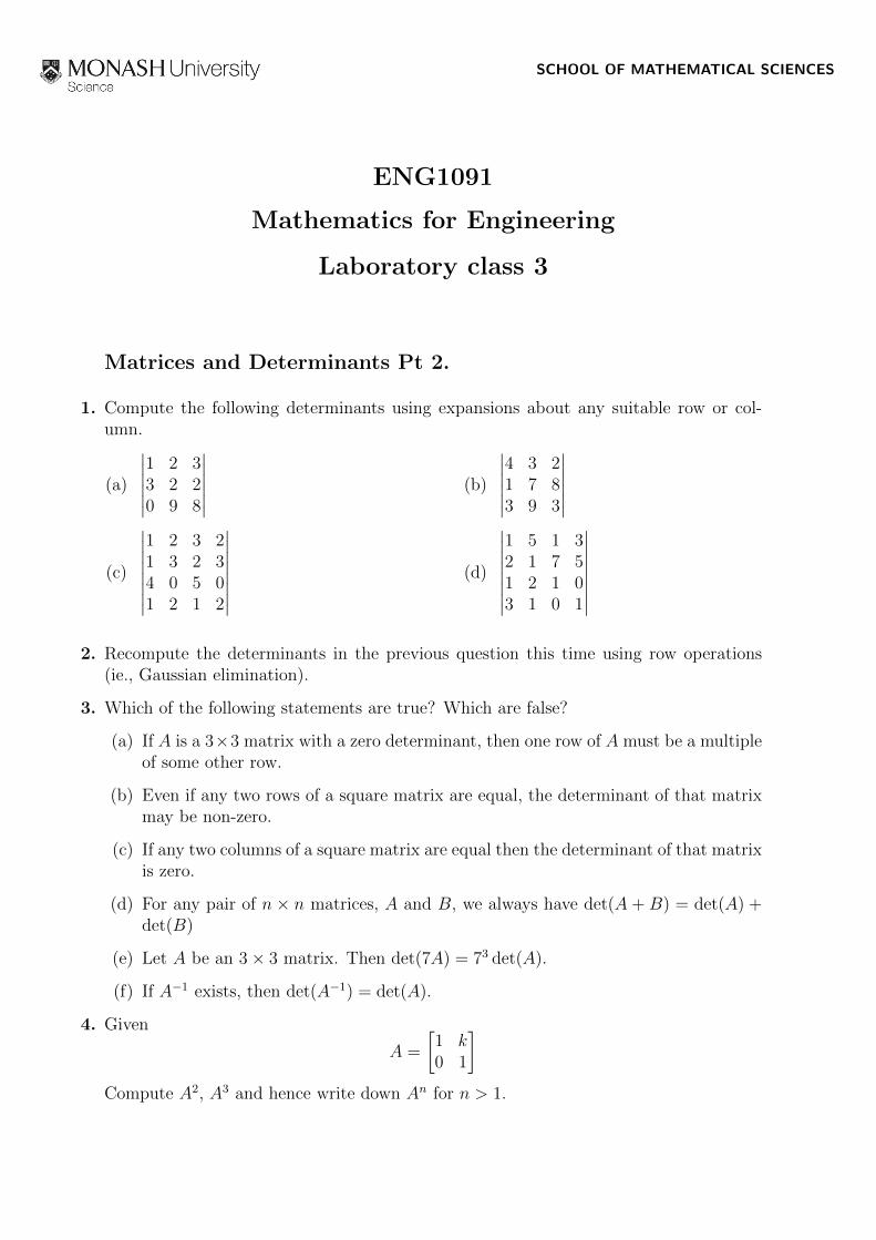
SCHOOL OF MATHEMATICAL SCIENCES
ENG1091
Mathematics for Engineering
Laboratory class 3
Matrices and Determinants Pt 2.
1. Compute the following determinants using expansions about any suitable row or col-umn.
(a)
∣∣∣∣∣∣1 2 33 2 20 9 8
∣∣∣∣∣∣ (b)
∣∣∣∣∣∣4 3 21 7 83 9 3
∣∣∣∣∣∣(c)
∣∣∣∣∣∣∣∣1 2 3 21 3 2 34 0 5 01 2 1 2
∣∣∣∣∣∣∣∣ (d)
∣∣∣∣∣∣∣∣1 5 1 32 1 7 51 2 1 03 1 0 1
∣∣∣∣∣∣∣∣2. Recompute the determinants in the previous question this time using row operations
(ie., Gaussian elimination).
3. Which of the following statements are true? Which are false?
(a) If A is a 3×3 matrix with a zero determinant, then one row of A must be a multipleof some other row.
(b) Even if any two rows of a square matrix are equal, the determinant of that matrixmay be non-zero.
(c) If any two columns of a square matrix are equal then the determinant of that matrixis zero.
(d) For any pair of n × n matrices, A and B, we always have det(A + B) = det(A) +det(B)
(e) Let A be an 3× 3 matrix. Then det(7A) = 73 det(A).
(f) If A−1 exists, then det(A−1) = det(A).
4. Given
A =
[1 k0 1
]Compute A2, A3 and hence write down An for n > 1.

School of Mathematical Sciences Monash University
5. Assume that A is square matrix with an inverse A−1. Prove that det(A−1) = 1/ det(A)
6. Let
A =
[5 22 1
]Show that
A2 − 6A+ I = 0
where I is the 2× 2 identity matrix. Use this result to compute A−1.
7. Consider the following pair of matrices
A =
11 18 7a 6 3−3 −5 −2
, B =
3 1 12b −1 −5−2 1 −6
Compute the values of a and b so that A is the inverse of B while B is the inverse of A.
8. Here is a 2× 2 matrix equation[a bc d
]=
[e fg h
] [p qr s
]Show that this is equivalent to the following sets of equations[
ac
]= p
[eg
]+ r
[fh
]and [
bd
]= q
[eg
]+ s
[fh
]9. Use the result of the previous question to show that if the original 2×2 matrix equation
is written asA = EP
then the columns of A are linear combinations of the columns of E.
10. Following on from the previous two questions, show that the rows of A can be writtenas linear combinations of the rows of P .
26-Jul-2014 192

SCHOOL OF MATHEMATICAL SCIENCES
ENG1091
Mathematics for Engineering
Laboratory class 3 Solutions
Matrices and Determinants Pt 2.
1. If possible, use a row or column that contains one or more zeros.
(a) 31 =
∣∣∣∣∣∣1 2 33 2 20 9 8
∣∣∣∣∣∣ (b) −165 =
∣∣∣∣∣∣4 3 21 7 83 9 3
∣∣∣∣∣∣(c) 0 =
∣∣∣∣∣∣∣∣1 2 3 21 3 2 34 0 5 01 2 1 2
∣∣∣∣∣∣∣∣ (d) 162 =
∣∣∣∣∣∣∣∣1 5 1 32 1 7 51 2 1 03 1 0 1
∣∣∣∣∣∣∣∣3. Which of the following statements are true? Which are false?
(a) False (b) False (c) True
(d) False (e) True (f) False
4. Compute A2 and A3 and note the pattern.
An =
[1 nk0 1
]
6.
A−1 = 6I − A =
[1 −2−2 5
]7. Require that AB = I and BA = I. Then a = 4 and b = −1.

SCHOOL OF MATHEMATICAL SCIENCES
ENG1091
Mathematics for Engineering
Laboratory class 4
Matrix operations
1. Suppose you are given a matrix of the form
R(θ) =
[cos θ − sin θsin θ cos θ
]Consider now the unit vector v
˜= [1, 0]T in a two dimensional plane. Compute R(θ)v
˜.
Repeat your computations this time using w˜
= [0, 1]T . What do you observe? Trythinking in terms of pictures, look at the pair of vectors before and after the action ofR(θ).
2. You may have recognised the two vectors in the previous question to be the familar basisvectors for a two dimensional space, i.e., i
˜and j
˜. We can express any vector as a linear
combination of i˜
and j
˜, that is
u˜
= a i˜
+ bj
˜for some numbers a and b. Given what you learnt from the previous question, what doyou think will be result of R(θ)u
˜? Your answer can be given in simple geometrical terms
(e.g., in pictures).
3. Give reasons why you expect R(θ + φ) = R(θ)R(φ). Hence deduce that
cos(θ + φ) = cos θ cosφ− sinφ sin θ
sin(θ + φ) = sin θ cosφ+ sinφ cos θ
4. Give reasons why you expect R(θ)R(φ) = R(φ)R(θ). Hence prove that the rotationmatrices R(θ) and R(φ) commute.
5. Show that detR(θ) = +1.
6. Given the above form for R(θ) write down, without doing any computations, the inverseof R(θ).

School of Mathematical Sciences Monash University
Eigenvectors and eigenvalues
A square matrix A has an eigenvector v with eigenvalue λ provided
Av = λv
The vector v would normally be written as a column vector. Its transpose vT is a rowvector.
The eigenvalues are found by solving the polynomial equation
0 = det(A− λI)
7. Compute the eigenvalues and eigenvectors of the following matrices.
(a)
[4 −25 −3
](b)
[6 1−3 2
](c)
[5 3−3 −1
]
8. Given that one eigenvalue is λ = −4, compute the remaining eigenvalues of the followingmatrices.
(a)
−1 3 −3√
2
3 −1 −3√
2
−3√
2 −3√
2 2
(b)
3 −1 −3√
2
−1 3 −3√
2
−3√
2 −3√
2 2
9. Compute the eigenvectors for each matrix of the previous question. Verify that the
eigenvectors of part (b) are mutually orthogonal (i.e., 0 = vT1 v2, 0 = vT1 v3 and 0 = vT2 v3).
10. Suppose the matrix A has eigenvectors v with corresponding eigenvalues λ. Show thatv is an eigenvector of An. What is its corresponding eigenvalue?
11. If λ, v are an eigenvalue-eigenvector pair for A then show that αv is also an eigenvectorof A.
12. Suppose the matrix A has eigenvectors v with corresponding eigenvalues λ. Deduce theeigenvectors and eigenvalues of R−1AR where R is a non-singular matrix.
13. Let A be any matrix of any shape. Show that ATA is a symmetric square matrix.
26-Jul-2014 195

SCHOOL OF MATHEMATICAL SCIENCES
ENG1091
Mathematics for Engineering
Laboratory class 4 Solutions
Matrix operations
1. Each of the vectors will have been rotated about the origin by the angle θ in a counter-clockwise direction.
2. The rotation observed in the previous question also applies to the general vector u˜
. ThusR(θ) is often referred to as a rotation matrix. Matrices like this (and their 3 dimensionalcounterparts) are used extensivly in computer graphics.
3. Any object rotated first by θ and then by φ could equally have been subject to a singlerotation by θ+φ. The resulting objects must be identical. Hence R(θ+φ) = R(θ)R(φ).
4. Regardless of the order in which the rotations have been applied the nett rotation willbe the same. Thus R(θ)R(φ) = R(φ)R(θ). Equally, you could have started by writingθ + φ = φ+ θ, then R(θ + φ) = R(φ+ θ) and so R(θ)R(φ) = R(φ)R(θ).
5.
detR(θ) =
∣∣∣∣cos θ − sin θsin θ cos θ
∣∣∣∣ = 1
6. The inverse of R(θ) is R(−θ).
Eigenvectors and eigenvalues
7. (a) λ = −1 and 2 (b) λ = 3 and 5 (c) λ = 2 (a double root)
8. (a) λ = 8 and − 4 (a double root) (b) λ = 8, 4 and − 4
9. In part (a) there is a double root λ = −4. In this case there are two linearly independenteigenvectors. Your may answers may appear different from those given here, you willneed to check that your eigenvectors are linear combinations of those given here. Also,remember that any scaling is allowed for an eigenvector.
(a) λ = 8 v = (−1,−1,√
2)T
λ = −4 v = (2, 0,√
2)T
λ = −4 v = (−1, 1, 0)T
(b) λ = 8 v = (−1,−1,√
2)T
λ = 4 v = (−1, 1, 0)T
λ = −4 v = (1, 1,√
2)T

School of Mathematical Sciences Monash University
10. The eigenvalue of An will be λn.
11. This is trivial, just multiply the eigenvalue equation Av = λv by α.
12. The matrix R−1AR will have λ as an eigenvalue with eigenvector R−1v.
13. Use (PQ)T = QTP T and (AT )T = A to show that (ATA)T = ATA. Hence ATA issymmetric.
26-Jul-2014 197
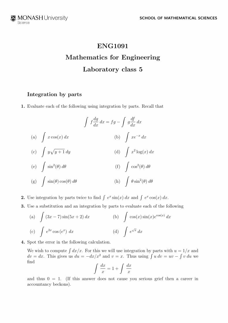
SCHOOL OF MATHEMATICAL SCIENCES
ENG1091
Mathematics for Engineering
Laboratory class 5
Integration by parts
1. Evaluate each of the following using integration by parts. Recall that
∫fdg
dxdx = fg −
∫gdf
dxdx
(a)
∫x cos(x) dx (b)
∫xe−x dx
(c)
∫y√y + 1 dy (d)
∫x2 log(x) dx
(e)
∫sin2(θ) dθ (f)
∫cos2(θ) dθ
(g)
∫sin(θ) cos(θ) dθ (h)
∫θ sin2(θ) dθ
2. Use integration by parts twice to find∫ex sin(x) dx and
∫ex cos(x) dx.
3. Use a substitution and an integration by parts to evaluate each of the following
(a)
∫(3x− 7) sin(5x+ 2) dx (b)
∫cos(x) sin(x)ecos(x) dx
(c)
∫e2x cos (ex) dx (d)
∫e√x dx
4. Spot the error in the following calculation.
We wish to compute∫dx/x. For this we will use integration by parts with u = 1/x and
dv = dx. This gives us du = −dx/x2 and v = x. Thus using∫u dv = uv −
∫v du we
find ∫dx
x= 1 +
∫dx
x
and thus 0 = 1. (If this answer does not cause you serious grief then a career inaccountancy beckons).

School of Mathematical Sciences Monash University
Improper integrals
5. Decide which of the following improper integrals will converge and which will diverge.
(a)
∫ 1
0
1
xdx (b)
∫ 1
0
1
x1/4dx
(c)
∫ 1
0
1
y4dy (d)
∫ ∞0
e−2x dx
(e)
∫ ∞0
1
1 + θ2dθ
Comparison test for Improper integrals
6. Use a suitable comparison function to decide which of the following integrals will convergeand which will diverge.
(a)
∫ 1
0
ex
xdx (b)
∫ 1
0
1
1− x1/4dx
(c)
∫ 1
0
e−y
y4dy (d)
∫ ∞0
sin2(x)e−2x dx
(e)
∫ ∞0
e−θ
1 + θ2dθ (f)
∫ 1
0
1
x(1− x2)dx
26-Jul-2014 199
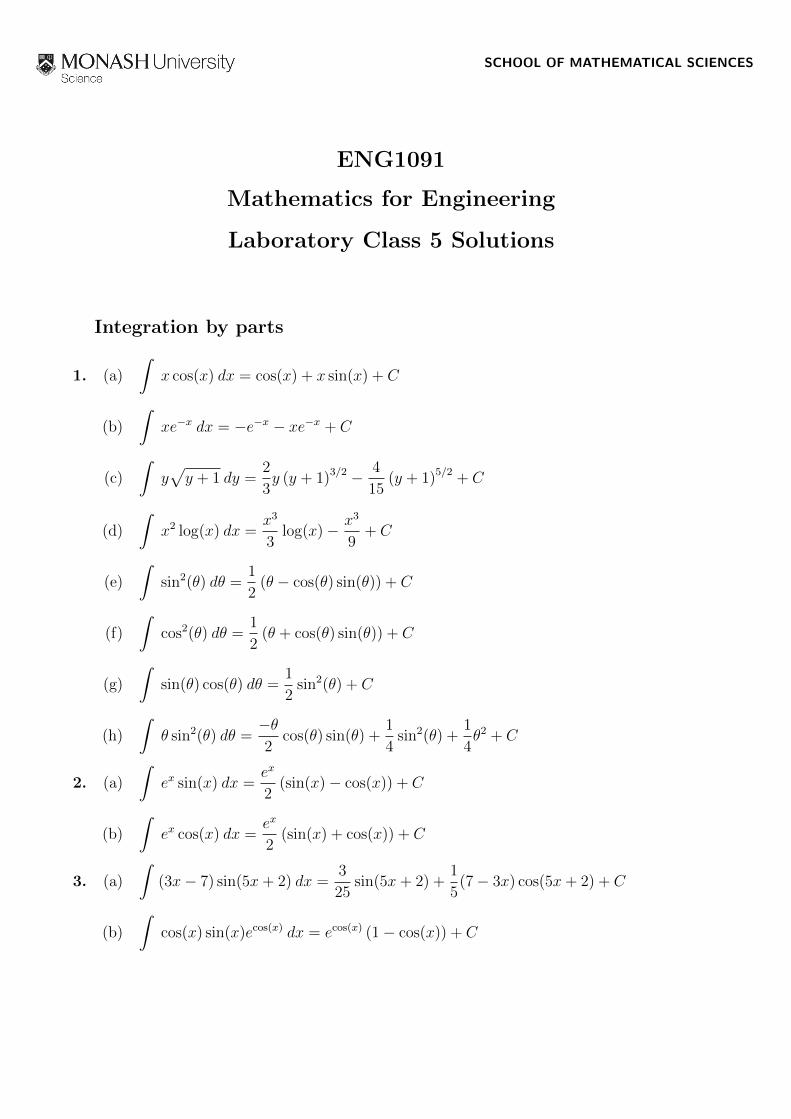
SCHOOL OF MATHEMATICAL SCIENCES
ENG1091
Mathematics for Engineering
Laboratory Class 5 Solutions
Integration by parts
1. (a)
∫x cos(x) dx = cos(x) + x sin(x) + C
(b)
∫xe−x dx = −e−x − xe−x + C
(c)
∫y√y + 1 dy =
2
3y (y + 1)3/2 − 4
15(y + 1)5/2 + C
(d)
∫x2 log(x) dx =
x3
3log(x)− x3
9+ C
(e)
∫sin2(θ) dθ =
1
2(θ − cos(θ) sin(θ)) + C
(f)
∫cos2(θ) dθ =
1
2(θ + cos(θ) sin(θ)) + C
(g)
∫sin(θ) cos(θ) dθ =
1
2sin2(θ) + C
(h)
∫θ sin2(θ) dθ =
−θ2
cos(θ) sin(θ) +1
4sin2(θ) +
1
4θ2 + C
2. (a)
∫ex sin(x) dx =
ex
2(sin(x)− cos(x)) + C
(b)
∫ex cos(x) dx =
ex
2(sin(x) + cos(x)) + C
3. (a)
∫(3x− 7) sin(5x+ 2) dx =
3
25sin(5x+ 2) +
1
5(7− 3x) cos(5x+ 2) + C
(b)
∫cos(x) sin(x)ecos(x) dx = ecos(x) (1− cos(x)) + C

School of Mathematical Sciences Monash University
(c)
∫e2x cos (ex) dx = cos(ex) + ex sin(ex) + C
(d)
∫e√x dx = 2e
√x(√
x− 1)
+ C
4. Did we forget an integration constant? (And so with the natural order restored, fears ofa career in accountancy fade from view.)
Improper integrals
5. Decide which of the following improper integrals will converge and which will diverge.
(a)
∫ 1
0
1
xdx diverges (b)
∫ 1
0
1
x1/4dx converges to 4/3
(c)
∫ 1
0
1
y4dy diverges (d)
∫ ∞0
e−2x dx converges to 1/2
(e)
∫ ∞0
1
1 + θ2dθ converges to π/2 (f)
∫ 2
0
1
1− x2dx diverges
(g)
∫ 2
0
1
x(x+ 2)dx diverges (h)
∫ 2
0
1
x(x− 2)dx diverges
Comparison test for Improper integrals
6. Use a suitable comparison function to decide which of the following integrals will convergeand which will diverge.
(a)
∫ 1
0
ex
xdx diverges, use
1
x<ex
xover 0 < x < 1
(b)
∫ 1
0
1
1− x1/4dx diverges, use x < x1/4 over 0 < x < 1
(c)
∫ 1
0
e−y
y4dy diverges, use
1
3y4<e−y
y4over 0 < y < 1
(d)
∫ ∞0
sin2(x)e−2x dx converges, use sin2(x)e−2x < e−2x over 0 < x <∞
(e)
∫ ∞0
e−θ
1 + θ2dθ converges, use
e−θ
1 + θ2<
1
1 + θ2over 0 < θ <∞
(f)
∫ 1
0
1
x(1− x2)dx diverges, use
1
x<
1
x(1− x2)over 0 < x < 1
26-Jul-2014 201
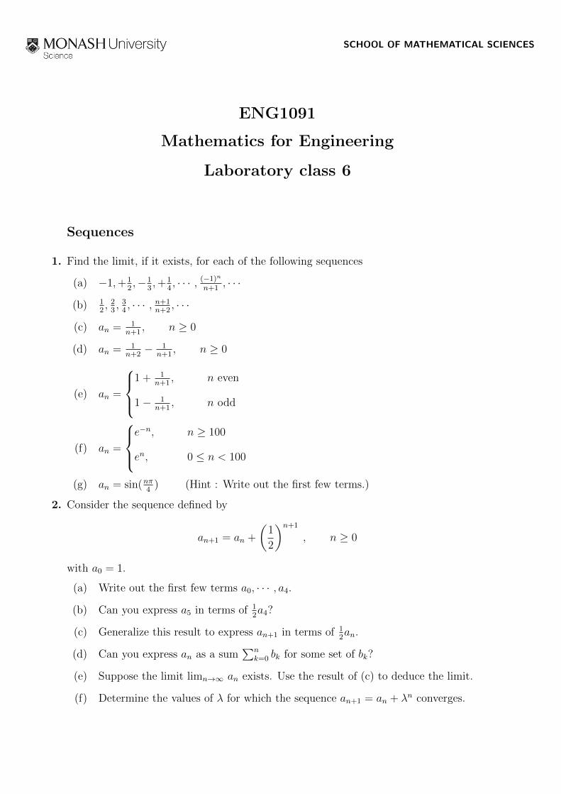
SCHOOL OF MATHEMATICAL SCIENCES
ENG1091
Mathematics for Engineering
Laboratory class 6
Sequences
1. Find the limit, if it exists, for each of the following sequences
(a) −1,+12,−1
3,+1
4, · · · , (−1)n
n+1, · · ·
(b) 12, 2
3, 3
4, · · · , n+1
n+2, · · ·
(c) an = 1n+1
, n ≥ 0
(d) an = 1n+2− 1
n+1, n ≥ 0
(e) an =
1 + 1
n+1, n even
1− 1n+1
, n odd
(f) an =
e−n, n ≥ 100
en, 0 ≤ n < 100
(g) an = sin(nπ4
) (Hint : Write out the first few terms.)
2. Consider the sequence defined by
an+1 = an +
(1
2
)n+1
, n ≥ 0
with a0 = 1.
(a) Write out the first few terms a0, · · · , a4.
(b) Can you express a5 in terms of 12a4?
(c) Generalize this result to express an+1 in terms of 12an.
(d) Can you express an as a sum∑n
k=0 bk for some set of bk?
(e) Suppose the limit limn→∞ an exists. Use the result of (c) to deduce the limit.
(f) Determine the values of λ for which the sequence an+1 = an + λn converges.

School of Mathematical Sciences Monash University
Series
3. Which of the following statements are true?
(a) The infinite series∑∞
n=0 an converges whenever limn→∞ |an| = 0.
(b) The harmonic series∑∞
n=0 1/(n+ 1) converges.
(c) If the series∑∞
n=0 |an| converges then∑∞
n=0 an also converges.
(d) If∑∞
n=0 an diverges then∑∞
n=0 (−1)nan converges.
(e) If limn→∞ |an+1
an| > 1 then
∑∞n=0 an converges.
The Integral Test
4. Establish the convergence (or divergence) of the following series using the integral test.
(a)∑∞
n=01√n+1
(b)∑∞
n=01
(n+1)γ, γ > 1
(c)∑∞
n=01
n2+1
(d)∑∞
n=01
(n+1)(n+2)
(Hint : First establish a comparison with∑∞
n=0 (n+ 1)−2 then use
the integral test.)
The Comparison Test
5. Determine the convergence or otherwise of the following series using the suggested seriesfor comparison.
(a)∑∞
n=0n+2n+1
compare with∑∞
n=0 1
(b)∑∞
n=01
(2+1/(n+1))n+1 compare with∑∞
n=01
2n+1
(c)∑∞
n=02+sinnn+1
compare with∑∞
n=01
n+1
(d)∑∞
n=03−n
n+1compare with
∑∞n=0
(13
)nThe Ratio Test
6. Use the ratio test to examine the convergence of the following series.
26-Jul-2014 203
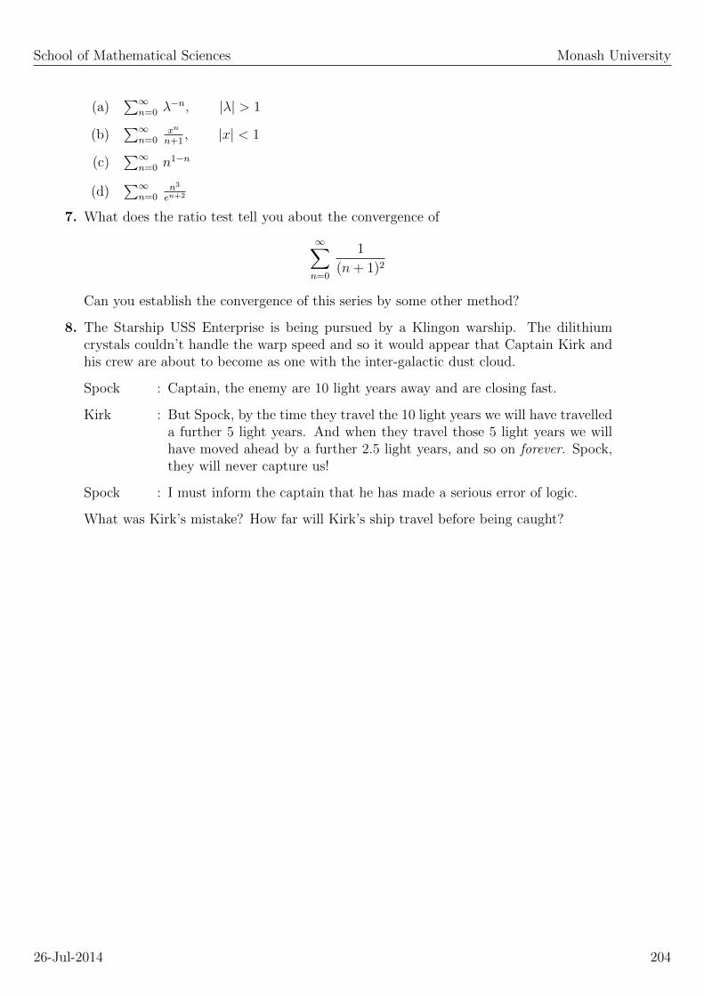
School of Mathematical Sciences Monash University
(a)∑∞
n=0 λ−n, |λ| > 1
(b)∑∞
n=0xn
n+1, |x| < 1
(c)∑∞
n=0 n1−n
(d)∑∞
n=0n3
en+2
7. What does the ratio test tell you about the convergence of
∞∑n=0
1
(n+ 1)2
Can you establish the convergence of this series by some other method?
8. The Starship USS Enterprise is being pursued by a Klingon warship. The dilithiumcrystals couldn’t handle the warp speed and so it would appear that Captain Kirk andhis crew are about to become as one with the inter-galactic dust cloud.
Spock : Captain, the enemy are 10 light years away and are closing fast.
Kirk : But Spock, by the time they travel the 10 light years we will have travelleda further 5 light years. And when they travel those 5 light years we willhave moved ahead by a further 2.5 light years, and so on forever. Spock,they will never capture us!
Spock : I must inform the captain that he has made a serious error of logic.
What was Kirk’s mistake? How far will Kirk’s ship travel before being caught?
26-Jul-2014 204

SCHOOL OF MATHEMATICAL SCIENCES
ENG1091
Mathematics for Engineering
Laboratory class 6 Solutions
Sequences
1. (a) 0 (b) 1 (c) 0 (d) 0(e) 1 (f) 0 (g) Limit does not exist
2. This is the geometric series. It converges for |λ| < 1.
Series
3. (a) False (b) False (c) True (d) False(e) False
The Integral Test
4. (a) Diverges (b) Converges (c) Converges (d) Converges
The Comparison Test
5. (a) Diverges (b) Converges (c) Diverges (d) Converges
The Ratio Test
6. (a) Converges (b) Converges (c) Converges (d) Converges
7. The series converges and this could also be established using the integral test.
8. Clearly the fast ship must catch the slow ship in a finite time. Yet Kirk has put anargument which shows that his slow ship will still be ahead of the fast ship after eachcycle (a cycle ends when the fast ship just passes the location occupied by the slow shipat the start of the cycle). Each cycle takes a finite amount of time. The total elapsedtime is the sum of the times for each cycle. Kirk’s error was to assume that the timetaken for an infinite number of cycles must be infinite. We know that this is wrong – aninfinite series may well converge to a finite number.

School of Mathematical Sciences Monash University
Given the information in the question we can see that the fast ship is initially 10 lightyears behind the slow ship and that it is traveling twice as fast as the slow ship. Supposethe fast ship is traveling at v light years per year. The distance traveled by the fast shipdecreases by a factor of 2 in each cycle. Hence the time interval for each cycle alsodecreases by a factor of 2 in each cycle. The total time taken will then be
Time =10 + 5 + 2.5 + 1.25 + ...
v
=10
v
(1 +
1
2+
1
4+
1
8· · ·)
=10
v
1
1− 12
=10
v/2
We expect that this must be time taken for the fast ship to catch the slow ship. Thefast ship is traveling at speed v while the slow ship is traveling at speed v/2. Thus thefast ship is approaching the slow ship at a speed v/2 and it is initially 10 light yearsbehind. Hence it will take the Klingon’s 10/(v/2) light years to catch Kirk’s starship.
26-Jul-2014 206

SCHOOL OF MATHEMATICAL SCIENCES
ENG1091
Mathematics for Engineering
Laboratory class 7
Power series
1. Find the radius of convergence for each of the following power series
(a) f(x) =∑∞
k=0kxk
3k(b) g(x) =
∑∞k=0
xk
3kk!
(c) h(x) =∑∞
k=0 k2xk (d) p(x) =
∑∞k=0
x2k
log(1+k)
(e) q(x) =∑∞
k=0k!(x−1)k
2kkk(f) r(x) =
∑∞k=0 (1 + k)kxk
Maclaurin Series
2. Find the first 4 non-zero terms in Maclaurin series for each of the following functions
(a) f(x) = cos(x) (b) f(x) = sin(2x)
(c) f(x) = log(1 + x) (d) f(x) = 11+x2
(e) f(x) = arctan(x) (f) f(x) =√
1− x2
3. Use the previous results to obtain the first 2 non-zero terms in the Maclaurin series forthe following functions.
(a) f(x) = cos(x) sin(2x) (c) f(x) = log(1 + x2)
(d) f(x) = 11+cos2(x)
(e) f(x) = arctan(arctan(x))
As the algebra in some parts of this question is rather tedious, you might like to do thisquestion using Scientific Notebook.

School of Mathematical Sciences Monash University
Taylor Series
4. Compute the Taylor series, about the the given point, for each of the following functions.
(a) f(x) = 1x, a = 1 (b) f(x) =
√x, a = 1
(c) f(x) = ex, a = −1 (d) f(x) = log x, a = 2
5. (a) Compute the Taylor series for ex
(b) Hence write down the Taylor series for e−x2
(c) Use the above to obtain an infinite series for the function
s(x) =
∫ x
0
e−u2
du
6. (a) Compute the Taylor series, around x = 0, for log(1 + x) and log(1− x).
(b) Hence obtain a Taylor series for f(x) = log(
1+x1−x
)(c) Compute the radius of convergence for the Taylor series in part (b).
(d) Show that the function defined by y(x) = 1+x1−x has a unique inverse for almost
all values of y.
(e) Use the above results to obtain a power series for log(y) valid for 1 < |y| <∞.
26-Jul-2014 208

SCHOOL OF MATHEMATICAL SCIENCES
ENG1091
Mathematics for Engineering
Laboratory class 7 Solutions
Power series
1. (a) R = 3 (b) R =∞(c) R = 1 (d) R = 1(e) R = 2e, note limn→∞(1 + x/n)n = ex (f) R = 0
Maclaurin Series
2. (a) cos(x) = 1− 12x2 + 1
24x4 − 1
720x6 + · · ·
(b) sin(2x) = 2x− 43x3 + 4
15x5 − 8
315x7 + · · ·
(c) log(1 + x) = x− 12x2 + 1
3x3 − 1
4x4 + · · ·
(d) 11+x2
= 1− x2 + x4 − x6 + · · ·
(e) arctan(x) = x− 13x3 + 1
5x5 − 1
7x7
(f)√
1− x2 = 1− 12x2 − 1
8x4 − 1
16x6 + · · ·
3. (a) cos(x) sin(2x) = 2x− 73x3 + · · · (c) log(1 + x2) = x2 − 1
4x4 + · · ·
(d) 11+cos2(x)
= 12
+ 14x2 + · · · (e) arctan(arctan(x)) = x− 2
3x3 + · · ·
Taylor Series
4. (a) 1x
= 1− (x−) + (x− 1)2 − (x− 1)3 + (x− 1)4 + · · ·
(b)√x = 1 + 1
2(x− 1)− 1
8(x− 1)2 + 1
16(x− 1)3 + · · ·
(c) ex = e−1(1 + (x+ 1) + 12(x+ 1)2 + 1
6(x+ 1)3 + · · ·
(d) loge x = loge(2) + 12(x− 2)− 1
8(x− 2)2 + 1
24(x− 2)3 + · · ·

School of Mathematical Sciences Monash University
5. (a) ex = 1 + x+ 12x2 + 1
6x3 + 1
24x4 + · · ·
(b) e−x2
= 1− x2 + 12x4 − 1
6x6 + 1
24x8 + · · ·
(c) s(x) =∫ x
0e−u
2= x− 1
3x3 + 1
10x5 − 1
42x7 + 1
216x9 + · · ·
6. (a) loge(1 + x) = x− 12x2 + 1
3x3 − 1
4x4 + · · · = ∑∞n=1
(−1)(n+1)
nxn
loge(1− x) = −x− 12x2 − 1
3x3 − 1
4x4 + · · · = −∑∞n=1
1nxn
(b) loge(
1+x1−x
)= 2x+ 21
3x3 + 21
5x5 + · · · = 2
∑∞n=1
12n−1
x2n−1, R = 1
(c) x = y−1y+1
, y 6= −1
(d) loge(y) = 2∑∞
n=11
2n−1x2n−1, x = (y − 1)/(y + 1)
26-Jul-2014 210
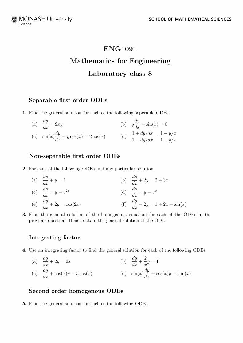
SCHOOL OF MATHEMATICAL SCIENCES
ENG1091
Mathematics for Engineering
Laboratory class 8
Separable first order ODEs
1. Find the general solution for each of the following seperable ODEs
(a)dy
dx= 2xy (b) y
dy
dx+ sin(x) = 0
(c) sin(x)dy
dx+ y cos(x) = 2 cos(x) (d)
1 + dy/dx
1− dy/dx =1− y/x1 + y/x
Non-separable first order ODEs
2. For each of the following ODEs find any particular solution.
(a)dy
dx+ y = 1 (b)
dy
dx+ 2y = 2 + 3x
(c)dy
dx− y = e2x (d)
dy
dx− y = ex
(e)dy
dx+ 2y = cos(2x) (f)
dy
dx− 2y = 1 + 2x− sin(x)
3. Find the general solution of the homogenous equation for each of the ODEs in theprevious question. Hence obtain the general solution of the ODE.
Integrating factor
4. Use an integrating factor to find the general solution for each of the following ODEs
(a)dy
dx+ 2y = 2x (b)
dy
dx+
2
xy = 1
(c)dy
dx+ cos(x)y = 3 cos(x) (d) sin(x)
dy
dx+ cos(x)y = tan(x)
Second order homogenous ODEs
5. Find the general solution for each of the following ODEs.

School of Mathematical Sciences Monash University
(a)d2y
dx2+dy
dx− 2y = 0 (b)
d2y
dx2− 9y = 0
(c)d2y
dx2+ 2
dy
dx+ 2y = 0 (d)
d2y
dx2+ 6
dy
dx+ 10y = 0
(e)d2y
dx2− 4
dy
dx+ 4y = 0 (f)
d2y
dx2+ 6
dy
dx+ 9y = 0
6. Find the particular solution, for the corresponding ODE in the previous question, thatsatisfies the following boundary conditions.
(a) y(0) = 1 and y(1) = 0 (b) y(0) = 0 and y(1) = 1
(c) y(0) = −1 and y(+π/2) = +1 (d) y(0) = −1 anddy
dx= 0 at x = 0
(e) y(0) = 1 anddy
dx= 0 at x = 1 (f)
dy
dx= 0 at x = 0 and
dy
dx=
1 at x = 1
Second order non-homogenous ODEs
7. Find the general solution for each of the following ODEs.
(a)d2y
dx2+dy
dx− 2y = 1 + x (b)
d2y
dx2− 9y = e3x
(c)d2y
dx2+ 2
dy
dx+ 2y = sin(x) (d)
d2y
dx2+ 6
dy
dx+ 10y = e2x cos(x)
(e)d2y
dx2− 4
dy
dx+ 4y = 2x (f)
d2y
dx2+ 6
dy
dx+ 9y = cos(x)
26-Jul-2014 212

SCHOOL OF MATHEMATICAL SCIENCES
ENG1091
Mathematics for Engineering
Laboratory class 8 Solutions
Separable first order ODEs
1. (a) y = Cex2
(b) y = ±√
2 cos(x) + C
(c) y = 2 +C
sin(x)(d) y =
C
x
Non-separable first order ODEs
2. (a) y = 1 (b) y =1
4+
3x
2
(c) y = e2x (d) y = xex
(e) y =1
4cos(2x) +
1
4sin(2x) (f) y = −1− x+
1
5cos(x) +
2
5sin(x)
3. (a) y = 1 + Ce−x (b) y =1
4+
3x
2+ Ce−2x
(c) y = e2x + Cex (d) y = xex + Cex
(e) y =1
4cos(2x) +
1
4sin(2x) + Ce−2x (f) y = −1− x+
1
5cos(x) +
2
5sin(x) +
Ce2x
Integrating factor
4. (a) y = x− 1
2+ Ce−2x (b) y =
x
3+C
x2
(c) y = 3 + Ce− sin(x) (d) y =C − loge(cos(x))
sin(x)

School of Mathematical Sciences Monash University
Second order homogenous ODEs
5. (a) y = Aex +Be−2x (b) y = Ae3x +Be−3x
(c) y = (A cos(x) +B sin(x)) e−x (d) y = (A cos(x) +B sin(x)) e−3x
(e) y = (A+Bx) e2x (f) y = (A+Bx) e−3x
6. (a) y(x) =1
e3 − 1
(e3−2x − ex
)(b) y(x) =
e3x − e−3x
e3 − e−3
(c) y(x) =(− cos(x) + eπ/2 sin(x)
)e−x (d) y(x) = − ((3 sin(x) + cos(x)) e−3x
(e) y(x) =
(1− 2x
3
)e2x (f) y(x) = −1
9(1 + 3x) e3−3x
Second order non-homogenous ODEs
7. (a) y = −3
4− x
2+ Aex +Be−2x
(b) y =(A+
x
6
)e3x +Be−3x
(c) y =1
5(−2 cos(x) + sin(x)) + (A cos(x) +B sin(x))e−x
(d) y =1
145(5 cos(x) + 2 sin(x)) e2x + (A cos(x) +B sin(x))e−3x
(e) y =1 + x
2+ (A+Bx)e2x
(f) y =1
50(4 cos(x) + 3 sin(x)) + (A+Bx)e−3x
26-Jul-2014 214
SCHOOL OF MATHEMATICAL SCIENCES
ENG1091
Mathematics for Engineering
Laboratory class 9
l’Hopital’s rule
1. Use l’Hopital’s rule to verify the following limits
(a) −2 = limx→−1
x2 − 1
x+ 1(b)
4
5= lim
x→0
sin(4x)
sin(5x)
(c)−1
π2= lim
x→1
1− x+ log(x)
1 + cos(πx)(d) 0 = lim
x→∞
log(log(x))
x
(e)1
4= lim
x→0
x
tan−1(4x)(f) 0 = lim
x→∞e−x log(x)
2. Prove that for any n > 00 = lim
x→∞xne−x
3. Prove that for any n > 00 = lim
x→∞x−n log(x)
Coupled first order ODEs
4. Solve each of the following coupled ODEs by first differentiating each equation andthen making suitable combinations to de-couple the equations. Verify your solutions bysubstituting back into the original ODEs.
(a)du
dx= 5u+ 3v
dv
dx= u+ 7v
(b)du
dx= 6u+ 3v
dv
dx= −4u− v
(c)du
dx= 4u− 2v
dv
dx= −u+ 3v
(d)du
dx= 8u+ 4v
dv
dx= −7u− 3v
5. Solve each of the coupled ODEs of the previous question by way of eigenvectors andeigenvalues.

SCHOOL OF MATHEMATICAL SCIENCES
ENG1091
Mathematics for Engineering
Laboratory class 10
Limits
1. At which points are the following functions discontinuous (if any)? Assume the domainfor each function to be R or R2.
(a) f(x) = sin(x) (b) g(x) = (2− x)/(2 + x)
(c) h(x) = log x (d) p(x) = (1 + 2x− x2)/(1 + 2x+ x2)
(e) r(x, y) = tan(x+ y) (f) s(x, y) = (x− y)2/(x+ y)2
(g) t(u, v) = (1 + u+ u2)/(1 + v + v2) (h) w(u, v) = exp(−u2 − v2)
2. Use your calculator to estimate the following limits.
(a) limx→0
sin(x)
x(b) lim
x→1
1 + x
1− x
(c) lim(x,y)→(0,0)
sin(x+ y)
x+ y(d) lim
(x,y)→(1,1)
(x+ y − 1)2
(x− y + 1)2
(e) lim(x,y)→(1,0)
x2 − y2 − 1
x2 + y2 − 1(f) lim
(x,y)→(0,0)
1− exp(−x2y2)
xy
Partial Derivatives
3. Evaluate the first partial derivatives for each of the following functions
(a) f(x, y) = cos(x) cos(y) (b) f(x, y) = sin(xy)
(c) f(x, y) = log(1 + x)/ log(1 + y) (d) f(x, y) = (x+ y)/(x− y)
(e) f(x, y) = xy (f) f(u, v) = uv(1− u2 − v2)
4. For the function f(x, y) = y2 sin(x) verify that
∂
∂x
(∂f
∂y
)=∂
∂y
(∂f
∂x
)

School of Mathematical Sciences Monash University
Chain Rule
5. Given f(x, y) = 2x2 + 4y − 2 and x(s) = 3s, y(s) = 2s2 compute df/ds by directsubstitution (i.e. first construct f(s)) and also by the chain rule.
6. Given f(x, y) = 2xy and x(r, θ) = r cos θ, y(r, θ) = r sin θ compute ∂f/∂x, ∂f/∂y,∂f/∂r and ∂f/∂θ,
7. Let f = f(x, y) be an arbitrary function of (x, y). Using the same transformation as inthe previous question express
∂2f
∂x2+∂2f
∂y2
in terms of partial derivatives of f in r and θ. This is a long and tedious question – havefun!
Directional derivatives
8. Compute df/ds for the function f(x, y) = xy + x+ y along the curve x(s) = r cos(s/r),y(s) = r sin(s/r). Also, verify that (dx/s) i
˜+ (dy/ds)j
˜is a unit vector.
9. Compute the directional derivative for each for the following functions in the stateddirection. Be sure that you use a unit vector!
(a) f(x, y) = 2x+ 3y at (1, 2), t˜
= (3 i˜
+ 4j
˜)/5
(b) g(x, y) = sin(x) cos(y) at (π/4, π/4), t˜
= ( i˜
+ j
˜)/√
2
(c) h(x, y, z) = log(x2 + y2 + z2) at (1, 0, 1), t˜
= i˜
+ j
˜− k˜
(d) q(x, y, z) = 4x2 − 3y3 + 2z2 at (0, 1, 2), t˜
= 2 i˜− 3j
˜+ k˜
(e) r(x, y, z) = z exp(−2xy) at (1, 1,−1), t˜
= i˜− 3j
˜+ 2k
˜(f) w(x, y, z) =
√1− x2 − y2 − z2 at (0.5, 0.5, 0.5), t
˜= 2 i
˜− j
˜+ k˜
Tangent planes
10. Compute the tangent plane f̃ approximation for each of the following functions at thestated point.
(a) f(x, y) = 2x+ 3y at (1, 2)
(b) g(x, y) = sin(x) cos(y) at (π/4, π/4)
(c) h(x, y, z) = log(x2 + y2 + z2) at (1, 0, 1)
(d) q(x, y, z) = 4x2 − 3y3 + 2z2 at (0, 1, 2)
(e) r(x, y, z) = z exp(−2xy) at (1, 1,−1)
(f) w(x, y, z) =√
1− x2 − y2 − z2 at (0.5, 0.5, 0.5)
26-Jul-2014 217

School of Mathematical Sciences Monash University
11. Use the result from the previous question to estimate the function at the stated points.Compare your estimate with that given by a calculator.
(a) f(x, y) at (1.1, 1.9) (b) g(x, y) at (3π/16, 5π/16)
(c) h(x, y, z) at (0.8, 0.1, 0.9) (d) q(x, y, z) at (0.1, 1.1, 1.9)
(e) r(x, y, z) at (0.8, 1.2,−1.1) (f) w(x, y, z) at (0.6, 0.4, 0.6)
12. This is more a question on theory rather than being a pure number question. It is thusnot examinable.
Consider a function f = f(x, y) and its tangent plane approximation f̃ at some pointP . Both of these may be drawn as surfaces in 3-dimensional space. You might ask –How can I compute the normal vector to the surface for f at the point P? And that isexactly what we will do in this question.
Construct f̃ at P (i.e write down the standard formula for f̃). Draw this as a surface inthe 3-dimensional space. This surface is a flat plane tangent to the surface for f at P(hence the name, tangent plane).
Given your equation for the plane, write down a 3-vector normal to this plane. Hencededuce the normal to the surface for the function f = f(x, y) at P .
13. Generalise your result from the previous question to surfaces of the form 0 = g(x, y, z).This question is also a non-examinable extension. But it is fun! (agreed?).
Maxima and Minima
14. Find all of the extrema (if any) for each of the following functions (you do not need tocharactise the extrema).
(a) f(x, y) = 4− x2 − y2 (b) g(x, y) = xy exp(−x2 − y2)
(c) h(x, y) = x− x3 + y2 (d) p(x, y) = (2− x2) exp(−y)
(e) q(x, y, z) = 4x2 + 3y2 + z2 (f) r(x, y, z) = arctan((x−1)2+y2+z2)
26-Jul-2014 218

SCHOOL OF MATHEMATICAL SCIENCES
ENG1091
Mathematics for Engineering
Laboratory class 10 Solutions
Limits
1. At which points are the following functions discontinuous (if any)? Assume the domainfor each function to be R or R2.
(a) None (b) x = −2
(c) x = 0 (d) x = −1
(e) x+ y = ±π/2,±3π/2,±5π/2 · · · (f) x+ y = 0
(g) None (h) None
2. Use your calculator to estimate the following limits.
(a) 1 (b) ∞
(c) 1 (d) 1
(e) No unique limit, try limits alongthe axes.
(f) 0
Partial Derivatives
3. Evaluate the first partial derivatives for each of the following functions
(a)∂f
∂x= − sin(x) cos(y)
∂f
∂y= − cos(x) sin(y)
(b)∂f
∂x= y cos(xy)
∂f
∂y= x cos(xy)
(c)∂f
∂x=
1
(1 + x) log(1 + y)
∂f
∂y=
− log(1 + x)
(1 + y) log2(1 + y)
(d)∂f
∂x=−2y
(x− y)2
∂f
∂y=
2x
(x− y)2
(e)∂f
∂x= y
∂f
∂y= x
(f)∂f
∂u= v(1− 3u2 − v2)
∂f
∂v= u(1− u2 − 3v2)

School of Mathematical Sciences Monash University
Chain Rule
5. df/ds = 52s
6. ∂f/∂x = 2y, ∂f/∂y = 2x, ∂f/∂r = 4r cos θ sin θ, ∂f/∂θ = 2r2(cos2 θ − sin2 θ),
7. This is not an easy question, two chocolate frogs if you got it right!
∂2f
∂x2+∂2f
∂y2=∂2f
∂r2+
1
r
∂f
∂θ+
1
r2
∂2f
∂θ2
Directional derivatives
8. df/ds = r(cos2(s/r)− sin2(s/r)
)− sin(s/r) + cos(s/r).
9. (a) 18/5 (b) 0
(c) 0 (d) 35/√
14
(e) −2 exp(−2)/√
14 (f) −2/√
6
Tangent planes
10. (a) f̃(x, y) = 8 + 2(x− 1) + 3(y − 2)
(b) f̃(x, y) = (1/2) + (1/2)(x− π/4)− (1/2)(y − π/4)
(c) f̃(x, y, z) = log 2 + (x− 1) + (z − 1)
(d) f̃(x, y, z) = 5− 9(y − 1) + 8(z − 2)
(e) f̃(x, y, z) = exp(−2)(−1 + 2(x− 1) + 2(y − 1) + (z + 1))
(f) f̃(x, y, z) = (1/2)− (x− (1/2))− (y − (1/2))− (z − (1/2))
11. The calculator’s answer is in brackets.
(a) 7.9 (7.900) (b) 0.304 (0.2397)
(c) 0.393 (0.3784) (d) 3.7 (3.267)
(e) -0.149 (-0.1613) (f) 0.4 (0.3464)
12. This question is not examinable.
For a surface written in the form z = f(x, y) the vector
N =
(∂f
∂x
)i˜
+
(∂f
∂y
)j
˜− k˜
is normal to the surface.
26-Jul-2014 220

School of Mathematical Sciences Monash University
13. This question is not examinable.
For a surface written in the form 0 = g(x, y, z) the vector
N = ∇g =
(∂g
∂x
)i˜
+
(∂g
∂y
)j
˜+
(∂g
∂z
)k˜
is normal to the surface.
Maxima and Minima
14. (a) (0, 0) (b) (0, 0) and the four points (±1/√
2,±1/√
2)
(c) (±1/√
3, 0) (d) None
(e) (0, 0, 0) (f) (1, 0, 0)
26-Jul-2014 221


![Uniform-in-time convergence of ... - Monash Universityusers.monash.edu/~jdroniou/articles/droniou-eymard_unif-deg-parab.pdflinear abstract parabolic equations. In [43] the authors](https://img.dokumen.tips/doc/110x75/5f1588b3ed6f992ffb2a25f9/uniform-in-time-convergence-of-monash-jdroniouarticlesdroniou-eymardunif-deg-parabpdf.jpg)


