Embed Size (px)
Citation preview

Eng. 6002 Ship Structures 1Hull Girder Response Analysis
L E C T U R E 8 : R E V I E W O F B E A M T H E O R Y ( D E F O R M A T I O N S )
Overview
In this lecture we will look at beam deformations caused by bending moments
We will also review the differential equations of beam theory and solve them using Maple
Deformations
In simple beam theory we make the assumption that only the bending moments cause distortions.
So we can assume that the beam is bent into a simple circular curve over any short length.

Deformations
The neutral axis (NA) does not stretch or contract. The upper and lower parts of the beam compress and/or stretch.
We can use the two known relationships
strain)-(stress
moment)-(stress
E
I
My
Deformations
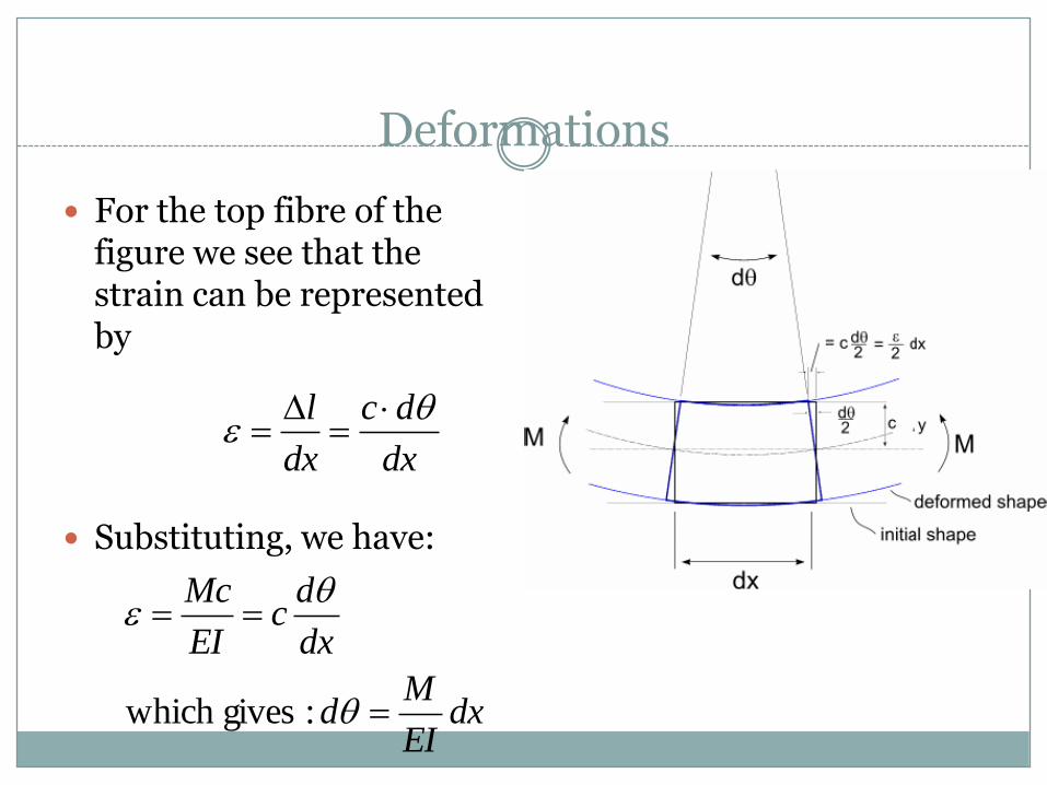
For the top fibre of the figure we see that the strain can be represented by
Substituting, we have:
dx
dc
dx
l
dxEI
Md
dx
dc
EI
Mc
:giveswhich
Deformations
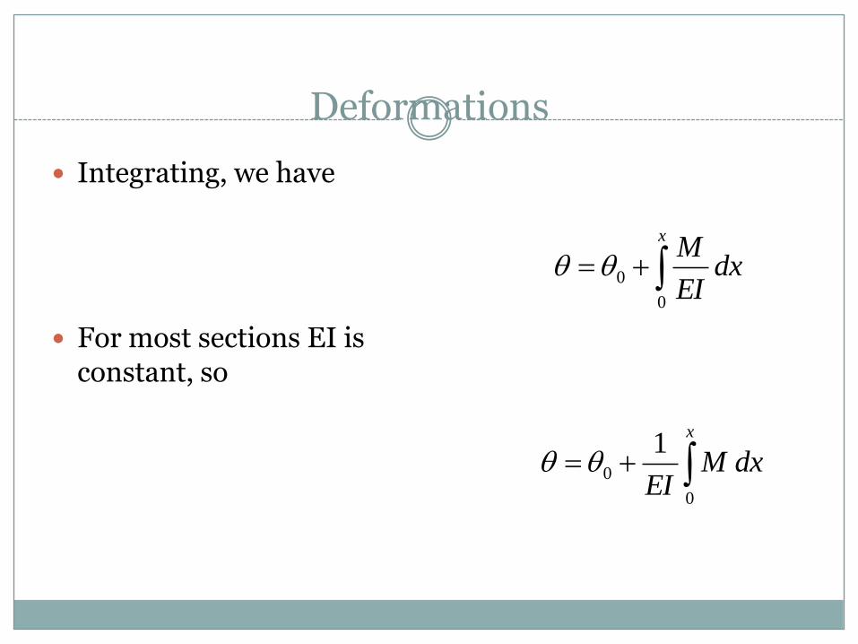
Integrating, we have
For most sections EI is constant, so
x
dxEI
M
0
0
x
dxMEI
0
0
1
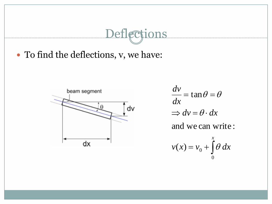
Deflections
To find the deflections, v, we have:
x
dxvxv
dxdv
dx
dv
0
0)(
:can write weand
tan
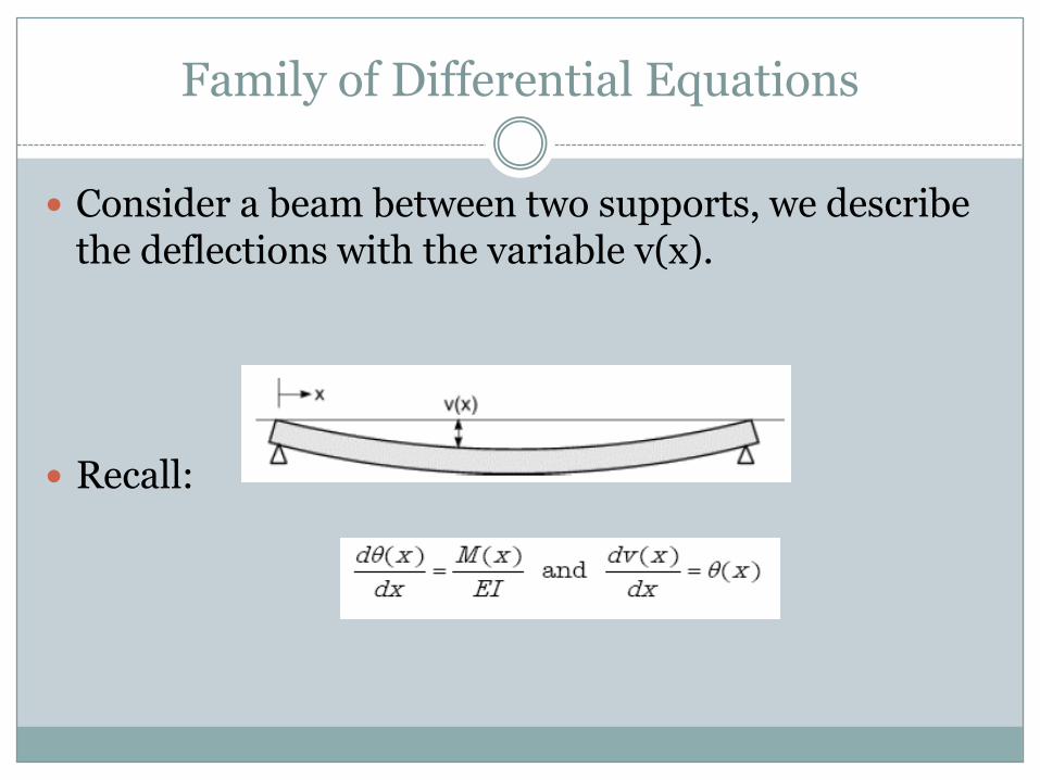
Family of Differential Equations
Consider a beam between two supports, we describe the deflections with the variable v(x).
Recall:
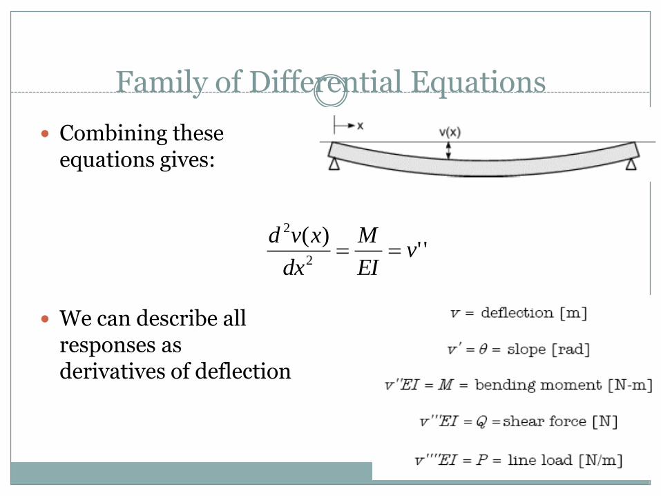
Family of Differential Equations
Combining these equations gives:
We can describe all responses as derivatives of deflection
'')(
2
2
vEI
M
dx
xvd

Family of Differential Equations
We can also express the relationships in integral form to give

Solving the Beam Equations
To solve beam equations, we need to know
the beam geometry and properties (L, E, I),
the loading conditions (length, shape and magnitude of load)
the boundary conditions (fixed, pinned, free, guided).
The boundary conditions are described in terms of what is known.
For a fixed end we know that the deflection and rotation are zero.
For a guided end we know that the shear (reaction) and rotation are zero.
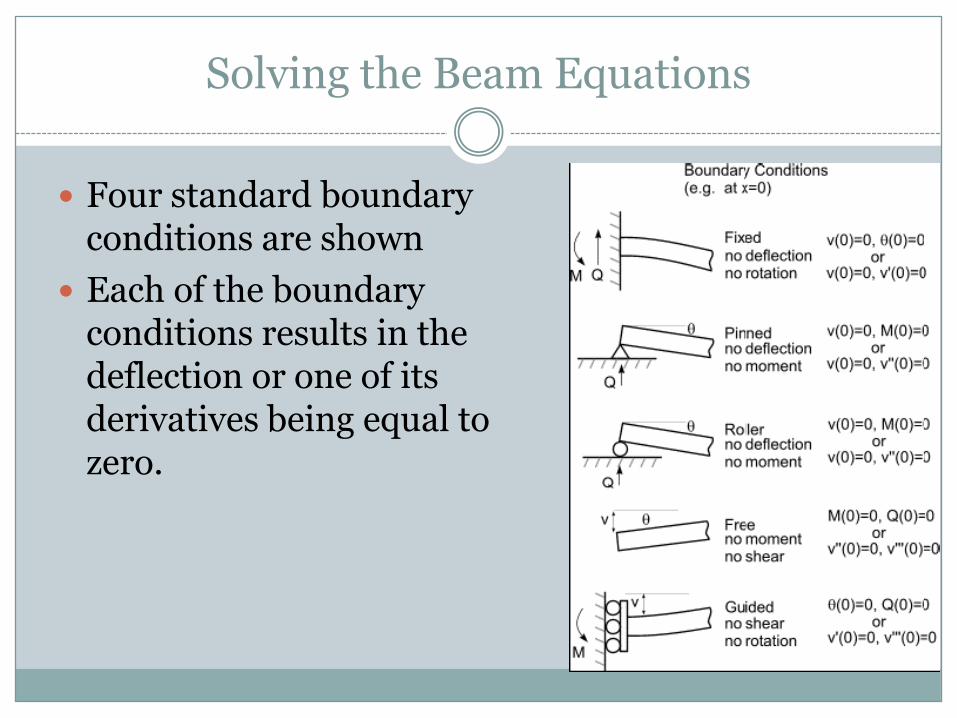
Solving the Beam Equations
Four standard boundary conditions are shown
Each of the boundary conditions results in the deflection or one of its derivatives being equal to zero.

Eng. 6002 Ship Structures 1Hull Girder Response Analysis
I N T R O D U C T I O N T O M A P L E

Overview
PURPOSE: To illustrate the use of dsolve to find exact solutions of many differential equations or systems of equations, with or without initial conditions.
NOTE 1. Maple has a powerful symbolic differential equation solver called dsolve. This command directs Maple to seek an exact symbolic expression for the solution of a given differential equation, or a system of differential equations, with or without initial conditions.
NOTE 2. Further information about dsolve can be obtained by issuing the command ‘?dsolve’.
Overview cont.
IMPORTANT NOTE: dsolve insists that coefficients be entered as rational, rather than floating point, numbers. For example, you should enter a coefficient as 1/2 or 1/4, rather than 0.5 or 0.2.
Example 1: A 1st order linear equation
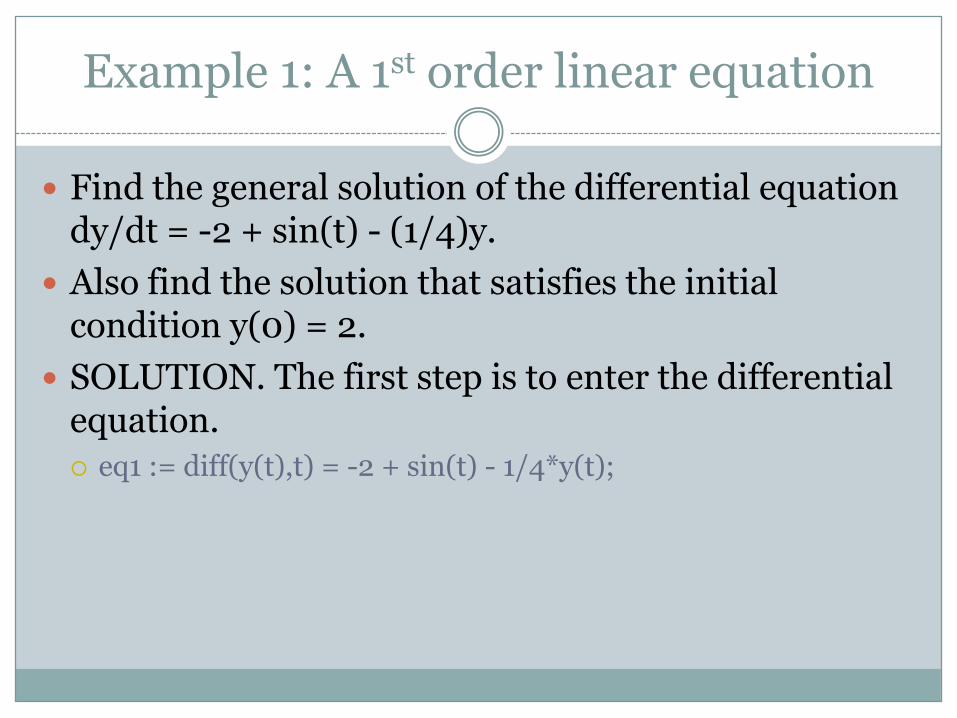
Find the general solution of the differential equation dy/dt = -2 + sin(t) - (1/4)y.
Also find the solution that satisfies the initial condition y(0) = 2.
SOLUTION. The first step is to enter the differential equation.
eq1 := diff(y(t),t) = -2 + sin(t) - 1/4*y(t);
Example 1: A 1st order linear equation
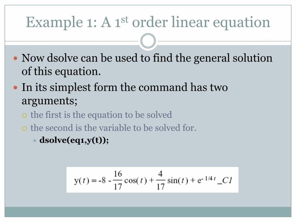
Now dsolve can be used to find the general solution of this equation.
In its simplest form the command has two arguments;
the first is the equation to be solved
the second is the variable to be solved for.
dsolve(eq1,y(t));

Example 1: A 1st order linear equation
This is the general solution of the given differential equation. Note that Maple writes the arbitrary constant as _C1, and that in this case the constant follows the term exp(-t/4) that it multiplies.
To find the solution that also satisfies the initial condition, we include the initial condition in the dsolve command, using braces to delimit the problem to be solved. Also we assign the name sol to the result.
sol := dsolve({eq1,y(0)=2},y(t));
Example 1: A 1st order linear equation
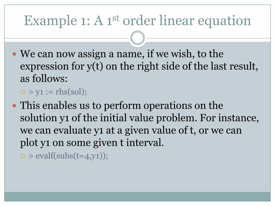
We can now assign a name, if we wish, to the expression for y(t) on the right side of the last result, as follows:
> y1 := rhs(sol);
This enables us to perform operations on the solution y1 of the initial value problem. For instance, we can evaluate y1 at a given value of t, or we can plot y1 on some given t interval.
> evalf(subs(t=4,y1));

Example 1: A 1st order linear equation
plot(y1,t=0..20);

Example 2: A 2nd order homogeneous linear equation
Solve the equation y’’ - 2y’ - 4y = 0.
Find the general solution and also the solution that satisfies the initial conditions y(0) = 2, y’(0) = -7/4.
SOLUTION: Again the first step is to enter the differential equation. In the following command note that the first term the second derivative is entered using t$2. This causes the differentiation operation to be executed twice.
eq2 := diff(y(t),t$2) - 2*diff(y(t),t) - 4*y(t) = 0;
dsolve(eq2,y(t));
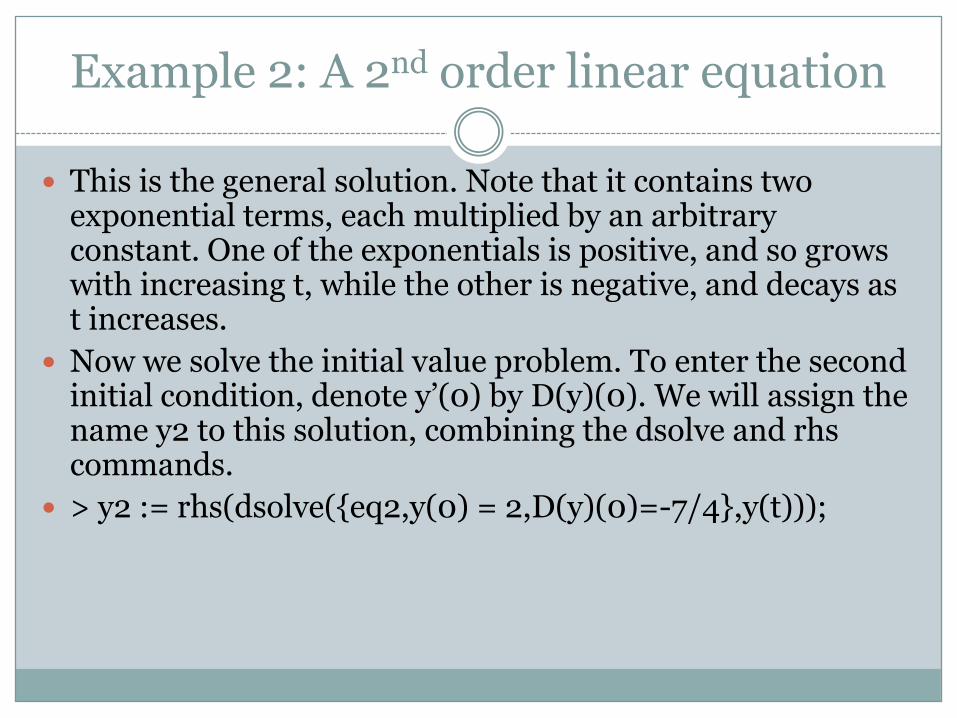
Example 2: A 2nd order linear equation
This is the general solution. Note that it contains two exponential terms, each multiplied by an arbitrary constant. One of the exponentials is positive, and so grows with increasing t, while the other is negative, and decays as t increases.
Now we solve the initial value problem. To enter the second initial condition, denote y’(0) by D(y)(0). We will assign the name y2 to this solution, combining the dsolve and rhs commands.
> y2 := rhs(dsolve({eq2,y(0) = 2,D(y)(0)=-7/4},y(t)));
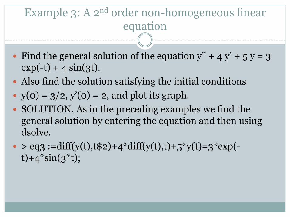
Example 3: A 2nd order non-homogeneous linear equation
Find the general solution of the equation y’’ + 4 y’ + 5 y = 3 exp(-t) + 4 sin(3t).
Also find the solution satisfying the initial conditions
y(0) = 3/2, y’(0) = 2, and plot its graph.
SOLUTION. As in the preceding examples we find the general solution by entering the equation and then using dsolve.
> eq3 :=diff(y(t),t$2)+4*diff(y(t),t)+5*y(t)=3*exp(-t)+4*sin(3*t);
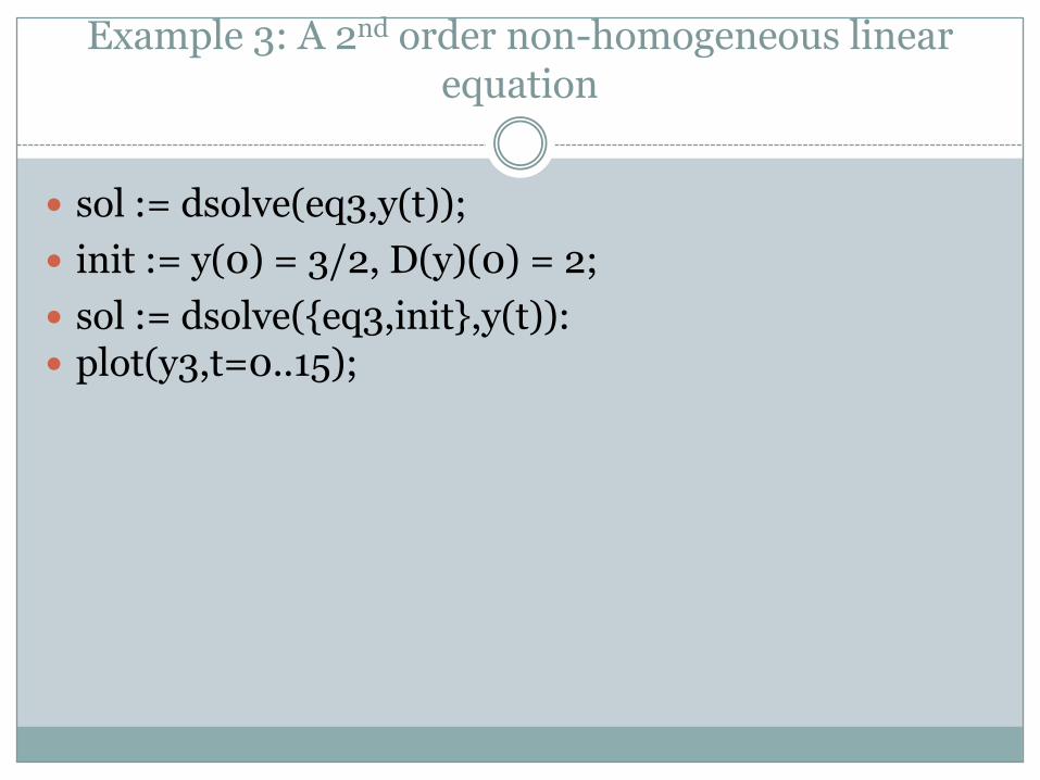
Example 3: A 2nd order non-homogeneous linear equation
sol := dsolve(eq3,y(t));
init := y(0) = 3/2, D(y)(0) = 2;
sol := dsolve({eq3,init},y(t)): plot(y3,t=0..15);
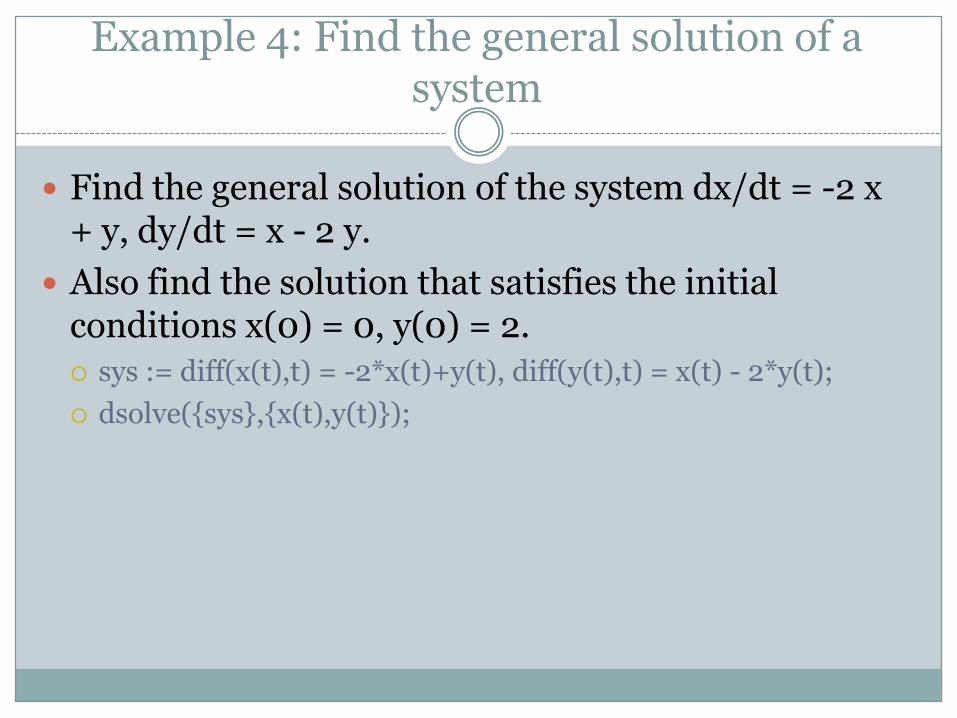
Example 4: Find the general solution of a system
Find the general solution of the system dx/dt = -2 x + y, dy/dt = x - 2 y.
Also find the solution that satisfies the initial conditions x(0) = 0, y(0) = 2.
sys := diff(x(t),t) = -2*x(t)+y(t), diff(y(t),t) = x(t) - 2*y(t);
dsolve({sys},{x(t),y(t)});

Example 4: Find the general solution of a system
Here is the solution of the initial value problem.
> dsolve({sys,x(0)=0,y(0)=2},{x(t),y(t)});

Ass 2
In each of the following problems use dsolve to find the general solution of the given differential equation. If initial conditions are given, also find the solution that satisfies them.
Plot this solution.
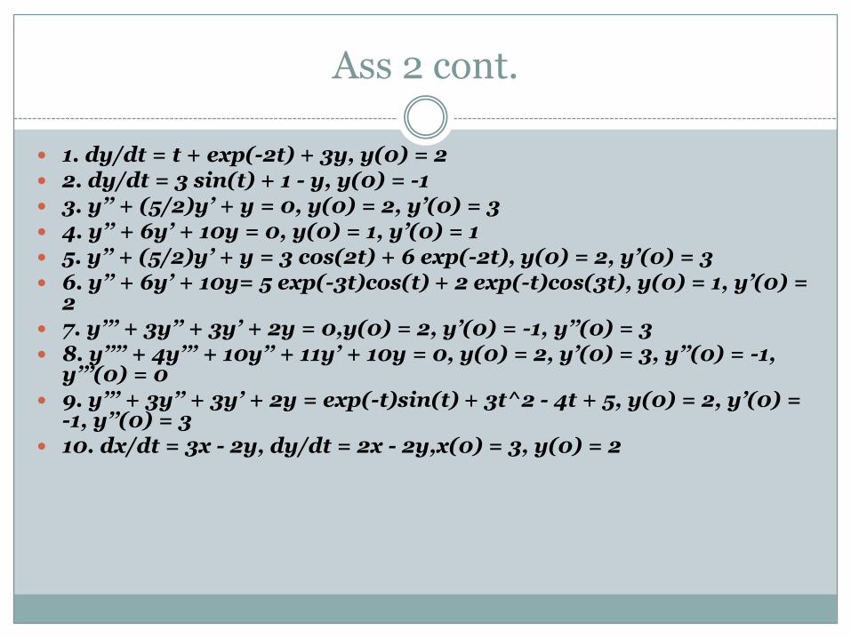
Ass 2 cont.
1. dy/dt = t + exp(-2t) + 3y, y(0) = 2 2. dy/dt = 3 sin(t) + 1 - y, y(0) = -1 3. y’’ + (5/2)y’ + y = 0, y(0) = 2, y’(0) = 3 4. y’’ + 6y’ + 10y = 0, y(0) = 1, y’(0) = 1 5. y’’ + (5/2)y’ + y = 3 cos(2t) + 6 exp(-2t), y(0) = 2, y’(0) = 3 6. y’’ + 6y’ + 10y= 5 exp(-3t)cos(t) + 2 exp(-t)cos(3t), y(0) = 1, y’(0) =
2 7. y’’’ + 3y’’ + 3y’ + 2y = 0,y(0) = 2, y’(0) = -1, y’’(0) = 3 8. y’’’’ + 4y’’’ + 10y’’ + 11y’ + 10y = 0, y(0) = 2, y’(0) = 3, y’’(0) = -1,
y’’’(0) = 0 9. y’’’ + 3y’’ + 3y’ + 2y = exp(-t)sin(t) + 3t^2 - 4t + 5, y(0) = 2, y’(0) =
-1, y’’(0) = 3 10. dx/dt = 3x - 2y, dy/dt = 2x - 2y,x(0) = 3, y(0) = 2
Eng. 6002 Ship Structures 1Hull Girder Response Analysis
L E C T U R E 9 : R E V I E W O F I N D E T E R M I N A T E B E A M S

Overview
The internal forces in indeterminate structures cannot be obtained by statics alone.
This is most easily understood by considering a similar statically determinate structure and then adding extra supports
This way also suggests a general technique for analyzing elastic statically indeterminate structures
Statically Indeterminate Beams
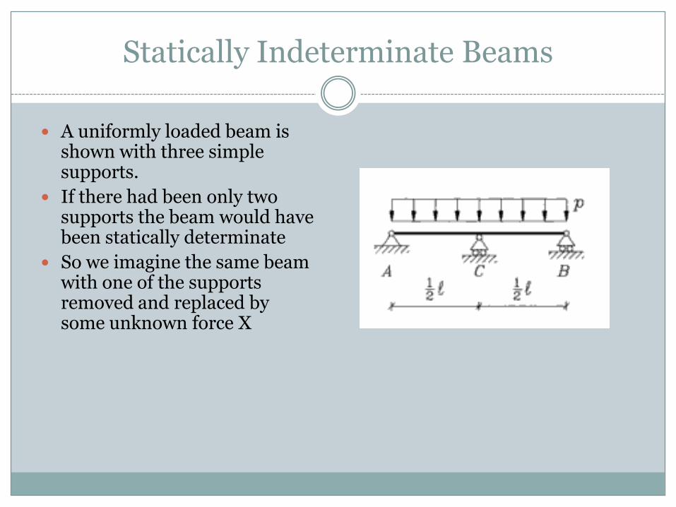
A uniformly loaded beam is shown with three simple supports.
If there had been only two supports the beam would have been statically determinate
So we imagine the same beam with one of the supports removed and replaced by some unknown force X
Statically Indeterminate Beams
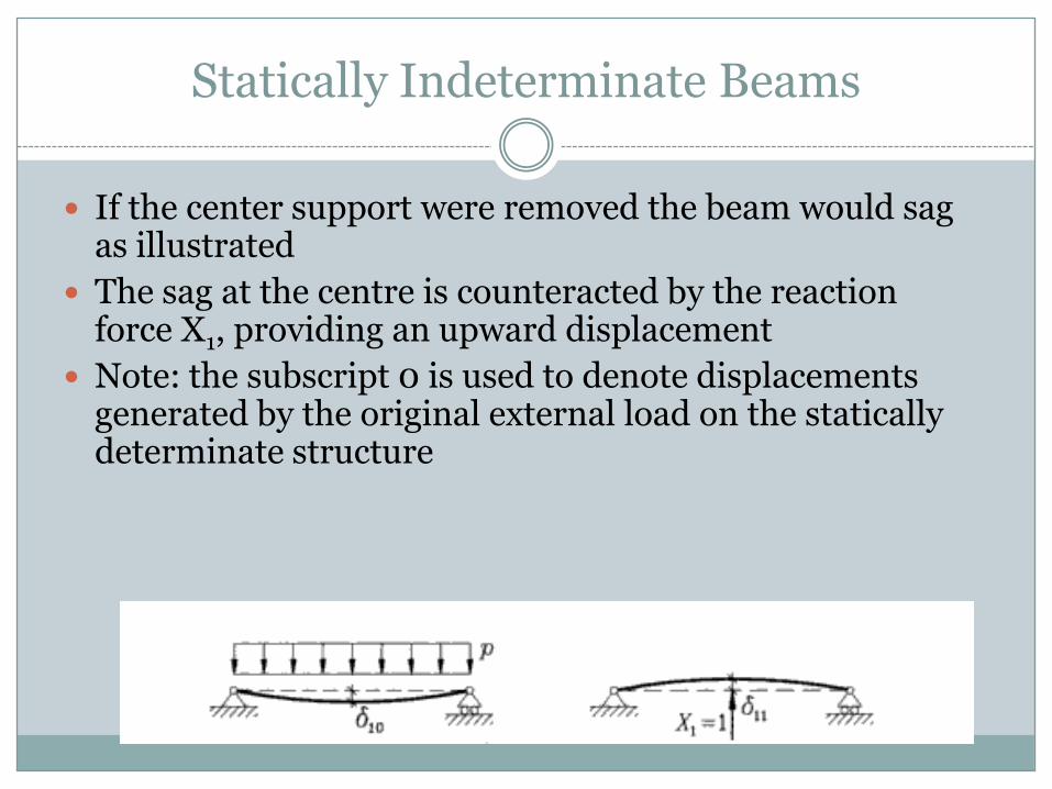
If the center support were removed the beam would sag as illustrated
The sag at the centre is counteracted by the reaction force X1, providing an upward displacement
Note: the subscript 0 is used to denote displacements generated by the original external load on the statically determinate structure
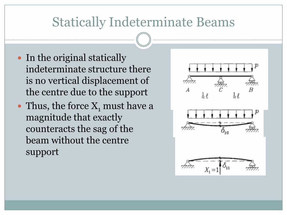
Statically Indeterminate Beams
In the original statically indeterminate structure there is no vertical displacement of the centre due to the support
Thus, the force X1 must have a magnitude that exactly counteracts the sag of the beam without the centre support
Statically Indeterminate Beams
There are two approaches for solving indeterminate systems. Both approaches use
the principle of superposition, by dividing the problem into two simpler problems,
solving the simpler problems and adding the two solutions.
The first method is called the Force Method (also called the Flexibility Method).
The idea for the force method is;

Statically Indeterminate Beams
The idea for the force method is:
Step 1. Reduce the structure to a statically determinate structure. This step allows the structure to displace where it was formerly fixed.
Step 2. solve each determinate system, to find all reactions and deflections. Note all incompatible deflections
Step 3. re-solve the determinate structures with only a set of self-balancing internal unit forces at removed reactions. This solves the system for the internal or external forces removed in 1.
Step 4. scale the unit forces to cause the opposite of the incompatible deflections
Step 5. Add solutions (everything: loads, reactions, deflections…) from 2 and 4.