Energy Savings Potential and Policy for Energy ... · PDF fileEnergy Savings Potential and Policy for Energy Conservation in Selected Indian Manufacturing Industries Manish Gupta and

Energy Savings Potential and Policy for Energy Conservation

in Selected Indian Manufacturing Industries

Manish Gupta and Ramprasad Sengupta

Working Paper No. 2012-105

September 2012

National Institute of Public Finance and Policy

New Delhi

http://www.nipfp.org.in

Energy Savings Potential and Policy for Energy

Conservation in Selected Indian Manufacturing

Industries

Manish Gupta* and Ramprasad Sengupta†

Abstract

Minimisation of damage from the rising trend of global warming would warrant two kinds of action for a country like India: a) abatement of greenhouse gas emissions and b) adaptation to climate change so as to reduce climate change related vulnerability of the people. The target of low carbon economic growth of India in terms of declining energy and carbon intensity of GDP assumes, therefore, a special significance in such context. Industrial sector being the largest consumer of final energy in India, the paper estimates the energy savings potential in seven major energy consuming industries for the period 2007-08. It further develops an econometric model admitting substitutability among energy and other non-energy inputs and between different fuels using translog cost function for the selected industries to study their behavioural response to changes in input prices and suggest policy instruments for conserving energy using time-series data for the period 1991-92 to 2008-09. The results of the model point mostly to the significant response of energy consumption to own price increases and to the insignificance of the responsiveness of the corresponding capital requirement to effect such energy conservation. Besides, a large part of the growth of factor productivity as estimated by the model has been found to be induced by energy price changes, the price neutral component of technical change being negligible. All these have important policy significance in respect of the relevance and direction of policy instruments for energy conservation in India for abating global warming. Keywords: Energy Conservation, Energy Efficiency, derived demand, elasticity, industry JEL Classification: Q41, Q43, Q48

* Manish Gupta (corresponding author) is Assistant Professor, National Institute of Public Finance

and Policy, New Delhi. Email: [email protected] † Ramprasad Sengupta is Visiting Professor, National Institute of Public Finance and Policy, New

Delhi and Distinguished Fellow, India Development Foundation, Gurgaon. (Formerly Sukhamoy Chakravarty Chair Professor of Development Planning, Centre for Economic Studies and Planning, Jawaharlal Nehru University, New Delhi)

Acknowledgement

The authors are grateful to M. Govinda Rao for his active interest and support. Discussions with him at various stages of the study were extremely helpful. The authors also would like to acknowledge discussions with Kavita Rao which were very useful. Chetana Choudhury provided excellent research assistance. Annual Survey of Industries data provided by the Ministry of Statistics and Programme Implementation is gratefully acknowledged. However, the usual disclaimers apply.

7

Energy Savings Potential and Policy for Energy

Conservation in Selected Indian Manufacturing

Industries

Introduction India is faced with the challenge of sustaining its rapid economic growth while

dealing with the threat of global climate change. Minimisation of damage from the rising trend of global warming would warrant two kinds of action for a country like India: a) abatement of greenhouse gas emissions; and b) adaptation to climate change by way of infrastructural and other developments to reduce climate change related vulnerability of the people. The National Action Plan on Climate change released in 2008 recognises the need to maintain high growth rate for raising the living standards of the vast majority of its people since higher income and higher level of infrastructural development can only reduce vulnerability of the people to adverse impacts of climate change. India’s development agenda thus focuses on the need for high inclusive economic growth for eradicating poverty and improving standards of living and reducing climate change related vulnerability of its people. In such a context the target of low carbon economic growth in terms of declining energy and carbon intensity of GDP, therefore, assumes special significance.

Of the different options for lowering carbon intensity of GDP, the option of energy conservation through reduced energy intensity of output (or value added) happens to be cheaper in most cases than the carbon free energy supply technology options. As the industrial sector has the largest sectoral share of final energy consumption in India accounting for about 47.6 per cent of the total commercial energy consumption in the country in 2007-08, the paper focuses on the assessment of the energy savings potential in this sector. More specifically the focus is on the seven major energy consuming industries namely, iron & steel, aluminium, paper & pulp, textiles, chlor-alkali, fertiliser, and cement. These industries are also the ones covered in the National Mission for Enhanced Energy Efficiency as part of the national initiative for addressing the problem of global climate change. These industries together account for about 46.5 per cent of final energy (measured in oil equivalent units) and 58.1 per cent of electricity (measured in kwh) consumed by the industrial sector, while their share in the industrial sector’s output and gross value addition is respectively 22.4 per cent and 27.6 per cent in 2007-08. Energy savings potential for each of these seven industries is assessed using firm level data from the Annual Survey of Industries (ASI) for the latest year available i.e., 2007-08.

Demand for inputs by industry is essentially a derived demand. A firm’s demand for inputs is derived from its output and factor prices. Since the firms prefer to choose input quantities which minimise their total cost of producing a given level of output, the derived demand for inputs would depend upon the substitution possibilities among inputs allowed by the technology, and the relative prices of all inputs. Since there is wide variation in energy consumption of individual industries caused partly by differences in the level of output and partly by differences in energy intensity which reflects variation in the underlying technology, it is reasonable to assume that the response of industries to changes in prices would be different. The paper develops an econometric model for inter-

8

input and inter-fuel substitution using translog cost function for each of the seven selected industries and also for the manufacturing sector of India as a whole to study the behavioural response of industries to changes in factor prices and thereby analyses possible role of the market based price or fiscal policy instruments for realising the assessed energy savings potential. In this assessment of both potential of energy conservation and the industry behaviour in response to price changes, we use time series data at the aggregate concerned industry level for the period 1991-92 to 2008-09 to obtain the most updated scenario compared to what is available in the literature.

The remainder of this paper is organised as follows: Section 2 provides a review of the literature on behavioural response of industries/manufacturing sector to changes in factor prices based on derived demand functions for factor inputs. Section 3 provides an assessment of energy savings potential in the selected energy consuming industries in India while section 4 presents an econometric model for inter-factor and inter-fuel substitution for these industries. Results of the model are presented in section 5. Section 6 discusses policy implications of the results in conserving energy in India’s manufacturing sector and relative efficacy of alternative market based instruments.

2. Review of Literature A large body of literature exists that have analysed the role of energy in the

structure of production. They provide estimates of derived demand elasticities for factor inputs using translog cost/production functions. Most have either used time series data for a single country's manufacturing sector or time series data pooled by country or manufacturing sub-sectors both in the developed and developing country context. Some of these studies have attempted to estimate the input demand functions for the manufacturing sectors of different countries by fitting aggregate translog cost function with three or four inputs namely capital (K), labour (L), energy (E), and materials (M) while others have attempted to estimate more disaggregated models with energy input disaggregated into different fuels or with fixed and working capital as separate capital inputs. Studies which have used energy as a single aggregate input include those by Berndt and Wood (1975), Hudson and Jorgenson (1974), Griffin and Gregory (1976), Magnus (1979), Ozatalay and Grubaugh (1979), Field and Grebenstien (1980). Studies by Fuss (1977), Griffin (1977), Halvorsen (1977) and Pindyck (1979) on the other hand have used energy in a disaggregated form and provide estimates of derived demand for aggregate energy input as well as for its different fuel constituents. All these studies were undertaken for developed countries. Absence of reliable data precluded similar type of analysis for the developing countries. Some of the studies for the developing country are by Pitt (1985) which uses firm-level cross-section data of manufacturing firms for Indonesia, and Roy et.al. (2006) which uses pooled data for US and three developing countries South Korea, Brazil, and India to estimate long-run substitution and price elasticities using factor inputs (KLEM) for selected industries.

In the Indian context also a large number of studies have quantified the energy

demand function and have estimated energy price responsiveness. Studies that have estimated input demand function using translog functions for Indian manufacturing sector include among others by Uri (1979), Williams and Laumas (1981), Apte (1983), Murty (1986), Kar and Chakraborty (1986), Roy (1992), Jha et al. (1993), Saha (1997).

9

Although there are many studies for India on inter-fuel and inter-factor substitution, not many have examined the bias in technical change towards energy or other non-energy factor inputs. Jha et al. (1993) is one of the first studies for India that examines technical change bias in the Indian manufacturing sector. Other studies that have examined technical change bias with respect to energy input in the Indian context are by Saha (1997) and Roy et al. (1999).

Most of these studies were carried out in response to the global oil crisis of 1973

and dealt with the possibilities of substitution of high cost fuel by relatively low cost one and substitution of energy with non-energy inputs for a given technological knowhow through the efficient utilisation of the concerned fuel. In the later phase of growing concern over climate change due to emissions from increased energy use, inter-fuel and inter-input substitution with the objective of energy conservation and lowering carbon intensity of GDP are finding renewed attention among policy makers globally. The present paper adds to the existing literature and addresses the issue of energy conservation in Indian manufacturing sector by exploring the relative efficacy of the market based policy instruments which would result in energy conservation in the manufacturing sector in India. Such energy conservation will not only result in a reduction of energy intensity of the economy but would also contribute towards lowering carbon intensity of not only the manufacturing sector but also of the entire economy thereby addressing the issue of abatement of global climate change. None of the existing studies which have analysed the role of energy in the structure of production in the Indian manufacturing sector have covered the period beyond 1993-94. It is well known that India initiated the process of economic reforms in 1991-92 during which the economy had undergone considerable changes. This process of economic reforms in India was also accompanied by reforms in the energy sector. The present study is probably the only study for India which explores the role of energy in the production structure in the post economic reforms period using time series data for the period 1991-92 to 2008-09 and explores the effectiveness of energy conserving policy instruments for the selected industries in India. Through this behavioural analysis the paper estimates the technical progress achieved by selected industries during the post-reform period and highlights their energy conserving character including the price responsiveness.

3. Energy Savings Potential As a first step, we obtain the energy savings potential for each of the seven

selected industries. Methodologically such an exercise involves use of efficiency benchmark of some of the best performing units within the concerned industry. Energy efficiency benchmarking for an industry is a process by which energy performance of an individual plant within the industry or a sector comprising of similar plants is compared against a common accepted best performance standard. The latter is decided by analysing the variation of performance metric across plants and their reasons leading to a criterion of best performance standard and value under the working condition of the plant or industry. As benchmarking is used as a tool for comparison it should have an important characteristic that the metric used should be independent of unit size. In the present study the metric used for benchmark analysis is energy intensity.

10

For the manufacturing sector in India the only available data source for carrying out such analysis is the unit level ASI data. We use the data for the latest year available i.e., 2007-08. There are, however, certain limitations of ASI data which delimit the scope of application of benchmark analysis discussed above. As the ASI data does not reveal the identity of different firms within an industry, it cannot be used for analysing the performance of different units over time. However, one can compare performance of different units within an industry vis-à-vis certain benchmark value.

There are a large number of units/firms of varying sizes within an industry. Comparing energy intensity of a small unit with that of large unit may not be meaningful because of the scale of operation. In order to overcome the problem of comparing dissimilar units, we have classified the units within an industry into different groups on the basis of a) share in final energy consumption (measured in kgoe); b) share in electricity consumption (measured in Kwh); and c) total output (measured in rupees), so that units within a group are similar in nature. We then calculate the energy savings potential for each group within the industry assuming technology to be related with any of these three measures of scale.

Having classified the units within an industry into different groups, units within a

group are ranked in order of their energy intensities. Energy intensity of a unit is defined as total final energy consumed for generating one unit of output. Since the output is measured in monetary units, energy intensity is defined as energy consumed for generating Re. 1 worth of output. Two measures of energy intensity have been used depending on the way in which the units are grouped. These are

Unit of energy intensity Definition of Energy Intensity

1 Classification based on Share of total energy consumption

a) Kgoe/Re ( )

( )

2 Classification based on Share of total electricity consumption

b) Kwh/Re ( )

( )

3 Classification based on Value of Output

a) Kgoe/Re ( )

( )

b) Kwh/Re ( )

( )

After having arranged the units within a group in order of their energy intensities, 10 per cent units that have the lowest energy intensity are selected and average energy intensity of these units is calculated. This average energy intensity of the top 10 per cent energy efficient units (i.e., the mean of the first decile of the energy intensity distribution within a group) is taken as the benchmark to which all the units within the group having energy intensity higher than the average were to achieve within a given period. Units which have energy intensity lower than the average continue to operate at their existing energy intensities. Energy consumption of all units having intensity higher than the benchmark is worked out using the benchmark energy intensity. However, for units which have energy intensity lower than the benchmark, their current energy consumption is considered. By adding the energy consumption of the two, modified overall energy consumption of the group is obtained. For a group the difference between its actual energy consumption and modified energy consumption worked out as discussed above is

11

obtained. The ratio of this difference in energy consumption and the actual energy consumption of a group gives its energy savings potential. Energy savings potential of different groups within the industry is calculated in a similar manner. Aggregating the energy savings potential of different groups within an industry we get the overall energy savings potential for the concerned industry.

Similar exercise is carried out i) by taking the lowest 25 per cent units as per

energy intensity criteria within a group and taking their average intensity (i.e., the mean of the first quartile of the energy intensity distribution) as the benchmark and ii) by taking the average intensity of units having energy intensity lower than the median energy intensity of the group (i.e., mean of the median of the energy intensity distribution) as the benchmark. Energy savings potential for each group is calculated and aggregating it across all groups gives the savings potential for the concerned industry.

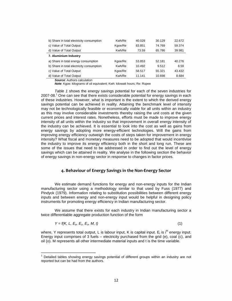
Table 1: Energy Savings Potential in Select Industries in India– 2007-08 Classification Based on Unit of

energy intensity

least energy

intensive 10% units

least energy

intensive 25% units

median energy

intensive units

1. Textile Industry

a) Share in total energy consumption Kgoe/Re 70.675 58.526 45.592

b) Share in total electricity consumption Kwh/Re 72.482 58.288 45.825

c) Value of Total Output Kgoe/Re 86.876 72.885 53.253

d) Value of Total Output Kwh/Re 88.233 73.764 53.629

2. Paper & Pulp Industry





3. Iron & Steel Industry





4. Fertiliser Industry





5. Chlor-Alkali Industry





6. Cement Industry


12




7. Aluminium Industry





Source: Authors calculation Note: Kgoe: kilograms of oil equivalent; Kwh: kilowatt hours; Re: Rupee

Table 1 shows the energy savings potential for each of the seven industries for 2007-08.1

One can see that there exists considerable potential for energy savings in each of these industries. However, what is important is the extent to which the derived energy savings potential can be achieved in reality. Attaining the benchmark level of intensity may not be technologically feasible or economically viable for all units within an industry as this may involve considerable investments thereby raising the unit costs at the given current prices and interest rates. Nonetheless, efforts must be made to improve energy intensity of all units within the industry so that improvement in overall energy intensity of the industry can be achieved. It is essential to look into the cost as well as gains from energy savings by adopting more energy-efficient technologies. Will the gains from improving energy efficiency outweigh the costs of steps taken for improvement in energy intensity? What fiscal and monetary measures need to be adopted that would incentivise the industry to improve its energy efficiency both in the short and long run. These are some of the issues that need to be addressed in order to find out the level of energy savings which can be attained in reality. We analyse in the following section the behavior of energy savings in non-energy sector in response to changes in factor prices.

4. Behaviour of Energy Savings in the Non-Energy Sector We estimate demand functions for energy and non-energy inputs for the Indian

manufacturing sector using a methodology similar to that used by Fuss (1977) and Pindyck (1979). Information relating to substitution possibilities between different energy inputs and between energy and non-energy input would be helpful in designing policy instruments for promoting energy efficiency in Indian manufacturing sector.

We assume that there exists for each industry in Indian manufacturing sector a twice differentiable aggregate production function of the form

Y = f(K, L, Ee, Ec, Eo, M, t) (1)

where, Y represents total output, L is labour input, K is capital input. Ei is i

th energy input.

Energy input comprises of 3 fuels – electricity purchased from the grid (e), coal (c), and oil (o). M represents all other intermediate material inputs and t is the time variable.

1 Detailed tables showing energy savings potential of different groups within an industry are not

reported but can be had from the authors.

13

Inclusion of time variable (t) as an argument in the production function implies the production relationship to change over time. We assume that the production function embodies constant returns to scale and is weakly separable in major categories of capital, labour, material, and energy. This assumption implies that the marginal rate of substitution between individual fuels is independent of the quantities of capital, labour. and material inputs. It is further assumed that capital, labour, material, and energy aggregates are homothetic in their components. In particular we assume that the energy aggregate is homothetic in its electricity, oil, and coal inputs. The last two assumptions are together referred to as homothetic separability assumption.2

Using the assumptions of homothetic separability, the production function (1) can be written as

Y = F[K, L, E(Ee, Ec, Eo), M, t] (2)

where, E is a homothetic function of the three fuels electricity, coal, and oil.

If factor prices and output levels are exogenously determined, the theory of duality between the cost and production implies that, given the cost minimising behaviour, production characteristics implied by equation (2) can be uniquely represented by a cost function which is also weakly separable. The cost function can be represented as

C = g[PL , PK , PE(PEe , PEc , PEo ), PM , t, Y) (3) where, C is the total cost, PL is the price of labour, PK is price of capital, PM price of material inputs, PEi is the price of i

th fuel. PE is the aggregate price of energy input. It is a

function that aggregates all individual fuels prices. The aggregator function is homothetic and does not include total quantity of energy as one of its arguments.

Homogeneity of degree one of the production function imply existence of a dual unit cost function giving output price as a function of input prices. Equation (3) can be written as

c = G[PL , PK , PM , PE(PEe , PEc , PEo ), t] (4)

where, c (=C/Y) is the unit cost

The unit cost function in (4) can be characterised and estimated in stages. In the first step we represent the price of energy, which is the unit cost of energy to a producer choosing fuel inputs which would minimise the total cost of energy, by a homothetic translog cost function with constant returns to scale. Estimation of the fuel share equations implied by this cost function gives the own and cross partial price elasticities for the three fuels considered, and the cost function itself provides an instrumental variable for the price of aggregate energy. In the next step we represent the cost of industrial output by a non-homothetic translog cost function. Estimation of the factor share equations implied by this cost function gives the price elasticity of demand and elasticity of factor substitution among the four inputs capital, labour, material, and energy (see Pindyck, 1979; and Fuss, 1977).

2 For a detailed discussion, see, Pindyck (1979)

14

We adopt a translog functional form for the unit cost function (4) as given below

( ) ( ) ∑

∑ ∑ ∑

(5)

where, i , j = K , L , E , M and .

For the cost function to be well behaved over the price range covered in the

sample, it must satisfy the properties of monotonicity, concavity and homogeneity. Linear homogeneity in input prices imply the following parametric restrictions

∑ ∑ ∑ ∑ (6)

The factor share equations can be derived from the unit cost function (5). We

make use of the Shephard’s lemma which implies

(7)

Since C = cY, we can write equation (7) as

Now consider ( )

( ) (

) (

) (8)

Substituting

, equation (8) can be written as

( )

( ) (

) (

)

, the cost share of the i

th input

and the input demand function, in terms of cost shares can be written as ∑ (9)

where i, j = K, L, E, M

The time variable t in the production function represents the way in which output

is affected by time. Following Hogan and Jorgenson (1991) and Sanstad et al. (2006), the rate of technical change is defined as

( )

, assuming all prices to remain unchanged (10)

i.e., the rate of technical change for each sector can be expressed as the negative of rate growth of unit cost or price of sectoral output with respect to time holding input prices constant. Using the unit cost function we can write equation (10) as

∑ (11) Symmetry of share equations and biases of productivity growth imply further

restrictions and (12)

Estimation of equations (9) and (11) requires them to be embedded within a

stochastic framework. This is done by adding a disturbance term in each of the four share

15

equations along with the technological change equation. Since the value shares sum to unity, the random disturbances in the four share equations for factor inputs are not independently distributed. However, from cross equation restrictions, we observe that any three value share equations, along with technological change equation, together yield estimates for all parameters. Since value shares sum to unity, the sum of disturbances across the four equations is zero at all observations. In order to avoid singularity of the covariance matrix any one of the share equations can be dropped and the remaining three can be estimated. The fourth share equation will be determined automatically. We drop capital share equation and the share equations represented by (9) are jointly estimated with the technical change equation (11), subject to the parametric restrictions in equations (12) and (6). Estimates are obtained by using the iterative Zellner-efficient estimation procedure. This estimation procedure is equivalent to full information maximum likelihood estimation (Pindyck, 1979).

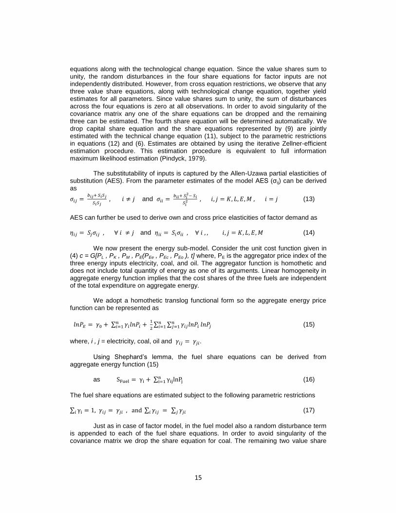
The substitutability of inputs is captured by the Allen-Uzawa partial elasticities of substitution (AES). From the parameter estimates of the model AES (σij) can be derived as

and

(13)

AES can further be used to derive own and cross price elasticities of factor demand as and (14)

We now present the energy sub-model. Consider the unit cost function given in

(4) c = G[PL , PK , PM , PE(PEe , PEc , PEo ), t] where, PE is the aggregator price index of the three energy inputs electricity, coal, and oil. The aggregator function is homothetic and does not include total quantity of energy as one of its arguments. Linear homogeneity in aggregate energy function implies that the cost shares of the three fuels are independent of the total expenditure on aggregate energy. We adopt a homothetic translog functional form so the aggregate energy price function can be represented as

∑

∑ ∑

(15)

where, i , j = electricity, coal, oil and .

Using Shephard’s lemma, the fuel share equations can be derived from

aggregate energy function (15) as ∑

(16)

The fuel share equations are estimated subject to the following parametric restrictions ∑ ∑ ∑ (17)

Just as in case of factor model, in the fuel model also a random disturbance term

is appended to each of the fuel share equations. In order to avoid singularity of the covariance matrix we drop the share equation for coal. The remaining two value share

16

equations are jointly estimated subject to the parametric restrictions specified by (17). Estimates were obtained using the iterative Zellner-efficient estimation procedure.

Substitutability of different fuels is captured by Allen-Uzawa partial elasticities of

substitution (AES) which is derived from the parameter estimates of the above model as

and

i, j = electricity, coal, oil (18)

Own and cross price elasticities of demand can be derive from AES as and (19)

However, these price elasticities are partial price elasticities when applied to

fuels. They account only for substitution between fuels, under the constraint that total quantity of energy consumed remains constant. However, the expenditure on energy will not remain constant. In fact, if the price of a particular fuel increases, its demand will decrease for two reasons, a) inter-fuel substitution resulting from changing relative fuel prices, and b) a decreased use of all energy resulting from an increase in the aggregate price of energy. The total own price elasticity for each fuel accounts for both inter-fuel substitution and the effect of a change in the price of the fuel on total consumption of energy. Thus, the total own and cross price elasticity of demand for each of the fuel is given by

and

(20)

The unit cost function is estimated in two stages. First, energy cost is minimised

in the choice of fuels (i.e., the inter-fuel model). Second, the total cost is minimised in the choice of factor inputs (i.e., the inter-factor model). The inter-fuel model provides

estimates of price of aggregate energy input ( ̂E) which is used as an instrumental variable for the price of energy in the estimation of the inter-factor model. Thus, we first estimate the homothetic translog fuel cost share equation (16) under the assumption of constant returns to scale subject to the parametric restrictions in equation (17). Parameters estimates of equation (16) are then used to compute the estimated energy

cost ( ̂E) using equation (15). The estimated value of the parameter in equation (15) is obtained under the assumption that for each industry under consideration PE = 1 in 1991-92 and the relative price index is calculated for all the years separately for different

industries. This estimated fuel cost or the unit price of aggregate energy ̂E is used as an instrumental variable for the aggregate price of energy (PE) while deriving estimates for the factor cost function given by equation (9).

The econometric analysis is carried out for the seven large energy consuming industries in India using ASI unit level data. Analysis has also been carried out by considering the entire manufacturing sector as a single category. The period of study is 18 years from 1991-92 to 2008-09.3

The initial year of the study, 1991-92, is significant as India embarked on the path of economic reforms in this year. The period of coverage of

3 For aluminium and chlor-alkali industries the analysis as for the period 1991-92 to 2007-08 as the

data for 2008-09 was not available in the form required for the study.

17

the study is thus the post economic reforms period during which the Indian economy had undergone considerable changes.

The price of the factor input labour (PL) required for the econometric model is

calculated as the ratio of wages and salaries including employers’ contribution to total number of persons engaged as given by ASI. The price of material inputs (PM) is calculated using the input-output tables for the year 2003-04 and the wholesale prices indices (at 1993-94 prices) of different inputs used in the production by the concerned industry. From the input-output tables, we get for the concerned industry the shares of different non-energy intermediate inputs that are consumed by the industry and using these shares as weights and the wholesale price indices of the non-energy intermediate inputs as prices, we get the price of the intermediate materials as the weighted average of wholesale price indices of different non-energy material inputs consumed by the industry.

Price of capital (PK) is calculated as PK = [(α*r)+{(1-α)*(r+d)}] where, PK is the

price of capital, (

), r is the rate of interest paid and is

calculated as the ratio of total interest paid to outstanding loan, d is the rate of depreciation and is the ratio of total depreciation to fixed capital. The data on working capital, fixed capital, depreciation, outstanding loans, interest paid is from the ASI.

ASI provides data on consumption of coal and electricity in both physical and monetary units. Consumption of coal and electricity is converted from their respective physical units into oil equivalent units by using fuel specific conversion factors. For electricity the conversion to oil equivalent units is in final energy terms. For each fuel dividing its consumption in oil equivalent terms by its consumption in value terms gives its price per oil equivalent unit of consumption. The information relating to consumption of different petroleum products is not adequate in ASI. It provides, information on consumption of different petroleum products both monetary and physical units till 1996-97. For later years however, it only provides information on the consumption of petroleum products as a group in monetary units only. We used the information provided by the Bureau of Energy Efficiency (BEE) on physical consumption of different petroleum products to derive for each industry the ratio in which different petroleum products are consumed by different industries. Using these ratios along with the price information relating to different petroleum products from the Indian Petroleum and Natural Gas Statistics and the fuel specific conversion factors for different distillates of oil we derive price per oil equivalent unit of petrol and petroleum products consumed by different industries.

5. Results The parameter estimates of the fuel model are given in table 2 while that of factor

model in table 2. Majority of the parameter estimates are statistically significant.4 Conventional goodness of fit is checked through R

2. For fuel share equations except for

4 60 out of 88 parameter estimates of the fuel model were significant either at 1, 5, or 10 percent

level while 133 out of 208 estimates are significant in case of the factor model.

18

few cases all R2 values are high ranging between 0.517 and 0.784. It is negative for the

oil share equation in case of cement industry. In case of factor model the R2 values are

high for all but seven cases ranging between 0.539 and 0.962. The technological change equation represented by equation (11) however, has low R

2 values.

Table 2: Parameter Estimates of the Fuel Model

Cement Paper & Pulp Fertiliser Iron & Steel

𝜸e 0.4230 *** 0.4494 *** 0.3204 *** 0.5737 ***

𝜸o 0.1212 *** 0.2091 *** 0.5398 *** 0.2092 ***

𝜸c 0.4558 *** 0.3415 *** 0.1398 *** 0.2172 ***

𝜸ee 0.1771 *** 0.0574

0.2008 *** 0.0663 *

𝜸eo -0.0715 *** -0.0727 *** -0.2468 *** -0.0292

𝜸ec -0.1056 *** 0.0153

0.0460

-0.0371

𝜸oe -0.0715 *** -0.0727 *** -0.2468 *** -0.0292

𝜸oo 0.0109

0.0822 *** 0.2648 *** 0.0524 **

𝜸oc 0.0605 ** -0.0095

-0.0180

-0.0232

𝜸ce -0.1056 *** 0.0153

0.0460

-0.0371

𝜸cc 0.0451

-0.0058

-0.0279

0.0603

R2electricity 0.7824 0.5728 0.7839 0.1481

R2oil -0.4161 0.5749 0.7689 0.2847

Textiles Aluminium Chlor-Alkali All Mfg

𝜸e 0.6721 *** 0.6084 *** 0.5871 *** 0.3378 ***

𝜸o 0.2682 *** 0.1652 *** 0.2465 *** 0.3582 ***

𝜸c 0.0597 *** 0.2263 *** 0.1665 *** 0.3040 ***

𝜸ee 0.1130 *** 0.1118 *** 0.1836 *** 0.2888 ***

𝜸eo -0.0601 ** -0.0533 *** -0.1413 *** -0.0541

𝜸ec -0.0530 *** -0.0584 * -0.0424

-0.2347 ***

𝜸oe -0.0601 ** -0.0533 *** -0.1413 *** -0.0541

𝜸oo 0.0321

0.0366 *** 0.1388 *** 0.0625 *

𝜸oc 0.0280 *** 0.0168

0.0025

-0.0084

𝜸ce -0.0530 *** -0.0584 * -0.0424

-0.2347 ***

𝜸cc 0.0250

0.0417

0.0399

0.2432 ***

R2electricity 0.2148 0.3808 0.7484 0.7334

R2 oil 0.0445 0.5167 0.5199 0.1542

Note: e = electricity; o = oil; c = coal ***, **, * represent level of significance at 1, 5 and 10 per cent respectively.

19

Table 3: Parameter Estimates of the Factor Model Cement Paper & Pulp Fertiliser Iron & Steel

al 0.0372 *** 0.0651 *** 0.0448 *** 0.0377 ***

ae 0.2630 *** 0.1619 *** 0.1141 *** 0.0863 ***

am 0.5123 *** 0.5980 *** 0.6532 *** 0.6567 ***

ak 0.1876 *** 0.1751 *** 0.1880 *** 0.2193 ***

bll 0.0334 *** 0.0313

0.0290 *** 0.0413 ***

ble 0.0110 * 0.0089 ** -0.0064

0.0167 **

blm -0.0285 *** -0.0349 ** -0.0171 *** -0.0453 ***

blt -0.0027 *** -0.0013 *** -0.0035 *** -0.0027 ***

bel 0.0110 * 0.0089

-0.0064

0.0167 **

bee -0.0964 *** 0.0370 *** 0.0144

0.0613 ***

bem 0.2252 *** -0.0283 * -0.0075

-0.0565 ***

bet -0.0173 *** -0.0017 *** 0.0028

0.0010

bml -0.0285 *** -0.0349 *** -0.0171 *** -0.0453 ***

bme 0.2252 *** -0.0283 * -0.0075

-0.0565 ***

bmm -0.1354 *** 0.1071 *** 0.0614

0.1514 ***

bmt 0.0089 *** 0.0008

0.0035

0.0012

at -0.0878

-0.1521 * -0.1071

-0.0629

btl -0.0027 *** -0.0013 *** -0.0035 *** -0.0027 ***

bte -0.0173 *** -0.0017 *** 0.0028

0.0010

btm 0.0089 *** 0.0008

0.0035

0.0012

btk 0.0111 *** 0.0022

-0.0028

0.0005

btt -0.0034

0.0092

0.0006

-0.0059

bkl -0.0159 *** -0.0053 -0.0054 * -0.0127 ***

bke -0.1398 *** -0.0175 *** -0.0005 -0.0215 ***

bkm -0.0613 ** -0.0438 -0.0369 * -0.0497 ***

bkk 0.2169 *** 0.0666 * 0.0428 *** 0.0839 ***

R2Labour 0.7789 0.5394 0.6448 0.7763

R2Energy 0.7000

0.8243

0.0204

0.6563

R2Material 0.8746 0.4251 0.6217 0.7579

R2time 0.0350 0.0840 0.0018 0.0520


al 0.0974 *** 0.0424 *** 0.0562 *** 0.0700 ***

ae 0.0802 *** 0.2084 *** 0.1440 *** 0.0771 ***

am 0.6991 *** 0.5761 *** 0.6231 *** 0.7017 ***

ak 0.1232 *** 0.1731 *** 0.1766 *** 0.1512 ***

bll 0.0275 *** 0.0353 ** 0.0448 *** 0.0540 ***

20


ble 0.0212 *** 0.0308

-0.0212 * 0.0105 ***

blm -0.0400 *** -0.0706 *** -0.0162

-0.0434 ***

blt -0.0028 *** 0.0002

-0.0039 *** -0.0033 ***

bel 0.0212 *** 0.0308

-0.0212 * 0.0105 ***

bee 0.0373 *** -0.0479

-0.0582

-0.0032

bem -0.0413 *** 0.0239

0.0403

0.0274 ***

bet -0.0002

-0.0104 * 0.0004

-0.0048 ***

bml -0.0400 *** -0.0706 *** -0.0162

-0.0434 ***

bme -0.0413 *** 0.0239

0.0403

0.0274 ***

bmm 0.0899 *** 0.1357

0.0079

0.0228

bmt 0.0020

0.0075

0.0035

0.0124 ***

at -0.1238 *** 0.3268

1.2149

-0.1176 ***

btl -0.0028 *** 0.0002

-0.0039 *** -0.0033 ***

bte -0.0002

-0.0104 * 0.0004

-0.0048 ***

btm 0.0020

0.0075

0.0035

0.0124 ***

btk 0.0010

0.0027

0.0000

-0.0043 ***

btt 0.0039

0.0074

-0.0327

-0.0019

bkl -0.0086 0.0044 -0.0074 -0.0211 ***

bke -0.0172 ** -0.0069 0.0391 -0.0348 ***

bkm -0.0086 -0.0890 ** -0.0320 * -0.0069

bkk 0.0345 0.0916 *** 0.0003 0.0627 ***

R2Labour 0.8764 0.6116 0.4920 0.9624

R2Energy 0.7086

0.4855

0.0930

0.8324

R2Material 0.4375 0.3776 0.1686 0.9520

R2time 0.0658 0.0007 0.0015 0.0076

Note: l = labour; k = capital, m = intermediate material input; e = energy; t = time ***, **, * represent level of significance at 1, 5 and 10 per cent respectively

Having estimated the parameters of the fuel model, AES between different fuels (σii and σij) is calculated using equation (18). We also calculate partial own and cross price elasticities of demand between different fuels (ηii, and ηij) at the mean values of the shares of different fuels in respective industries using equation (19). The estimates of AES and partial own and cross price elasticities of demand are reported in appendix tables A1 and A2. The estimates of total own and cross price elasticities of demand for different fuels (η*ii, and η*ij) are derived from partial price elasticities using equation (20) at the mean values of the shares of different fuels in respective industries and are shown in table 4. Positive cross price elasticity indicates substitutability among fuels, while negative value implies complementarity. Table 5 shows the relationship between the different energy inputs based on the estimates of total price elasticities. One can see that for chlor-alkali and overall manufacturing sector the three fuels - electricity, coal, and oil are complements with each other. A rise in the price of one would result in a decrease in the demand for other. However, in iron and steel industry the three fuels are substitutes implying that an increase in price of one would be associated with an increased demand for the other and vice-versa.

21

Similarly from the parameter estimates of the factor model we derive the Allen elasticity of substitution

5 and own and cross price elasticities. All elasticities are

calculated at the mean of each factor share. These elasticities are partial price elasticities. From table 6, which shows the estimates of price elasticities, one can see, the own price elasticity estimates are all negative as expected with the exception of own price elasticity of capital in cement industry and that of labour in all manufacturing sector. The price elasticities are in most cases inelastic. The own price elasticity of aggregate energy is not only negative for the industries selected but is also significant with the exception of iron and steel industry where although negative, it is not significant.

Table 4: Total Own and Cross Price Elasticities (Fuel Model)


η*ee -0.6013 *** -0.6958 *** -0.1472 ** -0.4927 ***

η*ec -0.3535 *** 0.1715 *** 0.2139 *** 0.0802 *

η*eo -0.2078 *** -0.0765 *** -0.8268 *** 0.1135 **

η*ce -0.2811 *** 0.2127 *** 0.3989 *** 0.2109 **

η*cc -0.9851 *** -0.8821 *** -1.1727 *** -0.5657 ***

η*co 0.1037 *** 0.0686 *** 0.0138 0.0559

η*oe -0.5989 *** -0.1325 *** -0.3433 *** 0.2642 **

η*oc 0.3759 *** 0.0957 *** 0.0031 ** 0.0495

η*oo -0.9396 *** -0.5640 *** -0.4198 *** -0.6127 ***


η*ee -0.4934 *** -0.8929 *** -0.7116 *** -0.3202 ***

η*ec -0.0435 *** -0.1415

-0.1289 ** -0.5454 ***

η*eo 0.0545 -0.1233

-0.3883 *** -0.1216 ***

η*ce -0.3586 *** -0.3280

-0.3631 ** -1.1244 ***

η*cc -0.6357 *** -0.8686 *** -0.7963 *** 0.1730 ***

η*co 0.5118 *** 0.0390

-0.0694 -0.0359

η*oe 0.1201 -0.3756

-0.4884 *** -0.1431 ***

η*oc 0.1369 *** 0.0512

-0.0310 -0.0205

η*oo -0.7394 *** -0.8333 *** -0.7094 *** -0.8236 ***

Note: ***, **, * represent level of significance at 1, 5 and 10 per cent respectively; All elasticities are calculated at the mean of each fuel’s share in total energy e = electricity; o = oil; c = coal

5 Estimates of AES are reported in appendix table A3.

22

Table 5: Inter-Fuel Relationship

Industry Electricity-Coal Electricity-Oil Oil-Coal

Cement C C S

Paper & Pulp S C S

Fertiliser S C S

Iron & Steel S S S

Textiles C S S

Aluminium C C S

Chlor-Alkali C C C

All Manufacturing C C C

Note: C = complements; S = Substitutes.

Table 6: Own and Cross Price Elasticities – Factor Model


ηll -0.1238 -0.4315 *** -0.2251 *** -0.1147

ηlk -0.2250 * 0.0618

-0.0067 -0.1299 **

ηle 0.5140 *** 0.2899 *** -0.0464 0.4403 ***

ηlm -0.1653 0.0798 0.2782 * -0.1957 *

ηkl -0.0521 * 0.0259 -0.0020 -0.0504 **

ηkk 0.4314 * -0.4010 * -0.5434 *** -0.2131 **

ηke -0.5717 *** 0.0273 0.1136 -0.0669

ηkm 0.1925 0.3477 0.4318 *** 0.3304 ***

ηel 0.0856 *** 0.1228 *** -0.0156 0.2124 ***

ηek -0.4111 *** 0.0275 0.1278 -0.0831

ηee -1.1626 *** -0.6008 *** -0.7600 *** -0.2989

ηem 1.4880 *** 0.4505 *** 0.6479 ** 0.1697

ηml -0.0120 0.0077 0.0154 * -0.0134 *

ηmk 0.0605 0.0796 0.0799 *** 0.0583 ***

ηme 0.6504 *** 0.1021 *** 0.1066 ** 0.0241

ηmm -0.6989 *** -0.1894 *** -0.2019 *** -0.0690 ***


ηll -0.5717 *** -0.2331 -0.1807 0.0748

ηlk -0.0004 0.2248 * 0.0228 -0.2883 ***

ηle 0.3567 *** 0.7800 * -0.2073 0.2620 ***

ηlm 0.2154 ** -0.7718 * 0.3652 * -0.0486

ηkl -0.0003 0.0819 * 0.0091 -0.1367 ***

ηkk -0.5765 ** -0.1875

-0.8502 *** -0.3254 **

23


ηke -0.0699 0.1024 0.4171 *** -0.2491 ***

ηkm 0.6467 *** 0.0033 0.4240 * 0.7112 ***

ηel 0.3237 *** 0.2500 * -0.0800 0.2193 ***

ηek -0.0888 0.0901 0.4045 *** -0.4396 ***

ηee -0.4824 *** -1.1577 ** -1.2288 *** -0.9872 ***

ηem 0.2475 * 0.8177 0.9043 ** 1.2075 ***

ηml 0.0233 ** -0.0574 * 0.0336 * -0.0033

ηmk 0.0979 *** 0.0007 0.0980 * 0.1025 ***

ηme 0.0295 * 0.1899 0.2156 ** 0.0986 ***

ηmm -0.1508 *** -0.1331 -0.3472 *** -0.1978 ***

Note: 1) ***, **, * represent level of significance at 1, 5 and 10 per cent respectively; 2) l = labour; e = energy; k = capital; m = intermediate material input 3) Positive cross price elasticity estimates indicate substitutability among inputs

while negative estimates indicate complementarity.

From the estimates of cross-price elasticities one can make the following observations a) capital and intermediate material inputs are substitutes in the selected industries, b) energy and intermediate materials inputs are substitutes in all industries, c) labour and energy inputs are substitutes in all except fertiliser and chlor-alkali industries, and d) capital and labour are substitutes only in paper and pulp, aluminium and chlor-alkali industries (see, table 7)

Table 7: Inter-factor Relationship

Capital - Labour

Capital - Energy

Capital - Material

Labour - Energy

Labour - Material

Energy - Material

Cement C C S S C S

Paper & Pulp S S S S S S

Fertiliser C S S C S S

Iron & Steel C C S S C S

Textiles C C S S S S

Aluminium S S S S C S

Chlor-Alkali S S S C S S

All Manufacturing C C S S C S

Note: C = complements; S = Substitutes.

Negative own price elasticity estimates for energy input have far reaching

implications as far as carbon emissions are concerned. The estimate of the parameter bee

is positive in paper and pulp, fertiliser, iron and steel, and textile industries (refer, table 3). The positive estimates of bee for these four industries indicate that with rising energy prices the cost share of energy would increase. This coupled with negative own price elasticity of energy input in these industries indicate that although the share of energy cost in the total cost will increase due to an increase in the price of energy, there would be reduction in energy consumption in physical terms. This implies that energy price increase would reduce carbon emissions depending on the quantity of reduction in carbonous energy use in these four industries. However, for the remaining industries namely, cement, aluminium, chlor-alkali and all manufacturing for which bee is negative,

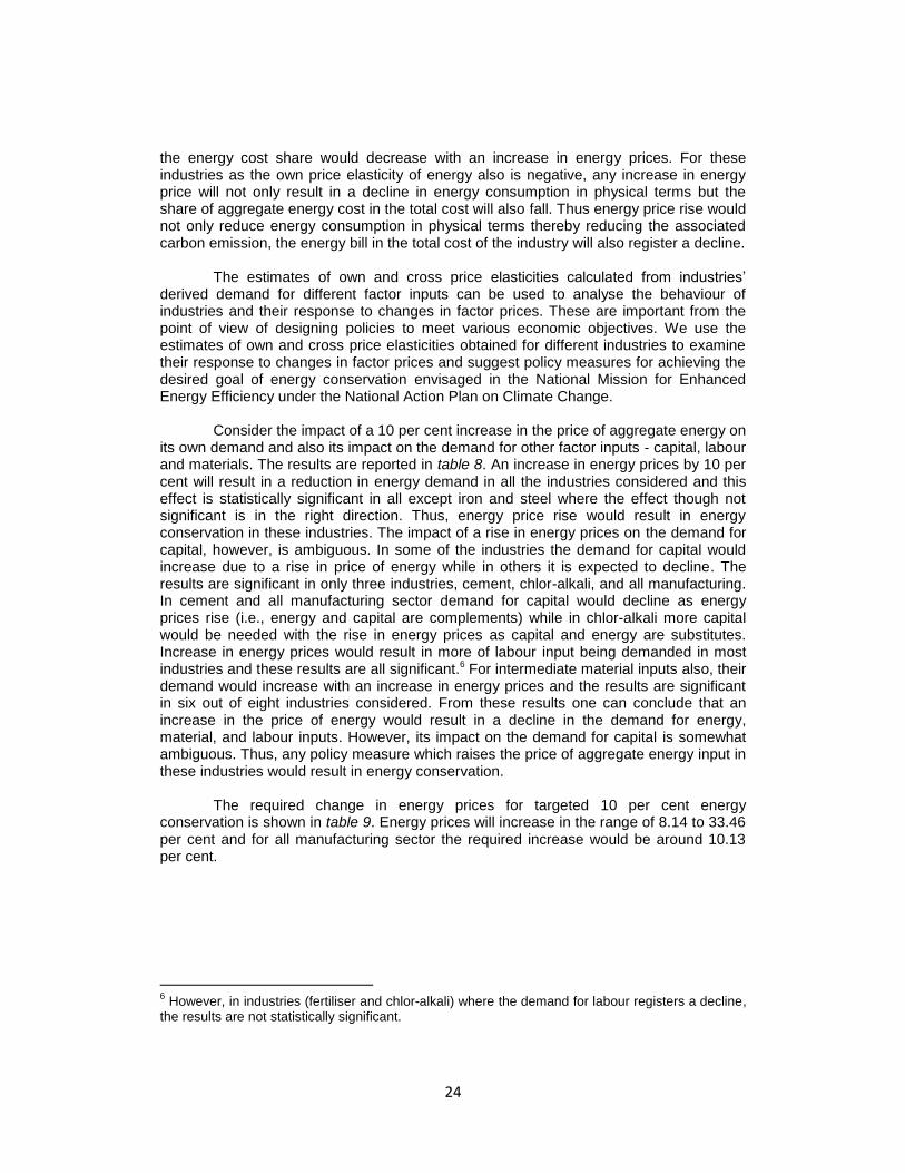
24

the energy cost share would decrease with an increase in energy prices. For these industries as the own price elasticity of energy also is negative, any increase in energy price will not only result in a decline in energy consumption in physical terms but the share of aggregate energy cost in the total cost will also fall. Thus energy price rise would not only reduce energy consumption in physical terms thereby reducing the associated carbon emission, the energy bill in the total cost of the industry will also register a decline. The estimates of own and cross price elasticities calculated from industries’ derived demand for different factor inputs can be used to analyse the behaviour of industries and their response to changes in factor prices. These are important from the point of view of designing policies to meet various economic objectives. We use the estimates of own and cross price elasticities obtained for different industries to examine their response to changes in factor prices and suggest policy measures for achieving the desired goal of energy conservation envisaged in the National Mission for Enhanced Energy Efficiency under the National Action Plan on Climate Change.

Consider the impact of a 10 per cent increase in the price of aggregate energy on its own demand and also its impact on the demand for other factor inputs - capital, labour and materials. The results are reported in table 8. An increase in energy prices by 10 per cent will result in a reduction in energy demand in all the industries considered and this effect is statistically significant in all except iron and steel where the effect though not significant is in the right direction. Thus, energy price rise would result in energy conservation in these industries. The impact of a rise in energy prices on the demand for capital, however, is ambiguous. In some of the industries the demand for capital would increase due to a rise in price of energy while in others it is expected to decline. The results are significant in only three industries, cement, chlor-alkali, and all manufacturing. In cement and all manufacturing sector demand for capital would decline as energy prices rise (i.e., energy and capital are complements) while in chlor-alkali more capital would be needed with the rise in energy prices as capital and energy are substitutes. Increase in energy prices would result in more of labour input being demanded in most industries and these results are all significant.6

For intermediate material inputs also, their demand would increase with an increase in energy prices and the results are significant in six out of eight industries considered. From these results one can conclude that an increase in the price of energy would result in a decline in the demand for energy, material, and labour inputs. However, its impact on the demand for capital is somewhat ambiguous. Thus, any policy measure which raises the price of aggregate energy input in these industries would result in energy conservation.

The required change in energy prices for targeted 10 per cent energy conservation is shown in table 9. Energy prices will increase in the range of 8.14 to 33.46 per cent and for all manufacturing sector the required increase would be around 10.13 per cent.

6 However, in industries (fertiliser and chlor-alkali) where the demand for labour registers a decline,

the results are not statistically significant.

25

Table 8: Percentage Change in Derived Demand for Energy & Consequent Changes in other

Factor Inputs for a 10 per cent Increase in Energy Price

Industries

Per cent change in

energy demand

Per cent change in

capital requirement

Per cent change in

labour requirement

Per cent change in material

requirement

Cement -11.626 *** -5.717 *** 5.140 *** 6.504 *** Paper & Pulp -6.008 *** 0.273 2.899 *** 1.021 *** Fertiliser -7.600 *** 1.136 -0.464 1.066 ** Iron & Steel -2.989 -0.669 4.403 *** 0.241 Textiles -4.824 *** -0.699 3.567 *** 0.295 * Aluminium -11.577 ** 1.024 7.800 * 1.899 Chlor-Alkali -12.288 *** 4.171 *** -2.073 2.156 ** All Manufacturing

-9.872 *** -2.491 *** 2.620 *** 0.986 ***

Note: Positive values indicate increase while Negative values indicate decrease ***; **; and * refers to significance at 1%, 5%, and 10% respectively

Table 9: Required Percentage Change in Energy Price for a 10% Reduction in Energy

Consumption Industries Change in

price of capital Industries Change in price of

capital

Cement 8.602 Textiles 20.728

Paper & Pulp 16.644 Aluminium 8.638

Fertiliser 13.157 Chlor-Alkali 8.138

Iron & Steel 33.456 All Manufacturing 10.129

Note: Positive values indicate increase while Negative values indicate decrease

We now consider the likely impact of changes in prices of different factor inputs

on their own demand and also on the demand for other inputs. Since the focus of the present study is on energy conservation, the analysis is restricted to analysing the impact of changes in prices of different factor inputs on energy demand7. Table 10 shows the percentage change in derived demand for capital and consequent changes in the demand for energy input for a 10 per cent Increase in the price of capital. A rise in the price of capital is associated with a fall in its own demand in all industries except cement where more demand for capital would increase as its price increases. These results are found to be significant in all industries except aluminium. The impact of a rise in price of capital on the demand for energy is ambiguous. The impact is significant only in three industries, chlor-alkali, cement, and all manufacturing. In chlor-alkali energy demand will increase with the rise in the price of capital, while in cement and all manufacturing sector, the demand for aggregate energy input will decrease as the price of capital increases. If one were to conserve energy, price of capital should decrease for chlor-alkali, while it should rise for cement and all manufacturing sector. Thus, there is no clear cut policy prescription for conserving energy through the capital price route. Provision of loans to industries at rates lower than the market rates which would lower their cost of capital so as to encourage them to invest in energy saving technology may not result in energy conservation and may therefore not be a good policy option.

7 Results relating to the requirement of other inputs due to changes in factor prices are not

reported.

26

Table 10: Percentage Change in Derived Demand for Capital and Consequent Changes in Energy

input for a 10 per cent Increase in the Price of Capital

Industries Per cent change in capital requirement

Per cent change in energy demand

Cement 4.314 * -4.111 *** Paper & Pulp -4.010 * 0.275 Fertiliser -5.434 *** 1.278 Iron & Steel -2.131 ** -0.831 Textiles -5.765 ** -0.888 Aluminium -1.875 0.901 Chlor-Alkali -8.502 *** 4.045 *** All Manufacturing -3.254 ** -4.396 ***


Table 11, derived from table 10, shows the percentage change in the price of capital required for a 10 per cent reduction in energy demand in each of the selected industries. For the three industries for which the results are significant, price of capital should decline by 24.72 per cent in chlor-alkali. However, for cement and all manufacturing sector, conservation of energy by 10 per cent would require the price of capital to increase by 24.32 and 22.75 per cent respectively. Table 11: Percentage Change in the Price of Capital for a 10 per cent Decrease in Energy Demand

Industries Change in price of capital

Industries Change in price of capital

Cement 24.32 Textiles 112.64 Paper & Pulp -362.99 Aluminium -111.05 Fertiliser -78.27 Chlor-Alkali -24.72 Iron & Steel 120.29 All Manufacturing 22.75

Note: Positive changes indicate increase while negative changes indicate decrease

The impact of a 10 per cent increase in the real wages (i.e., price of labour) on its own demand and the demand for aggregate energy input is shown in table 12. A rise in the price of labour results in a decrease in its own demand in the selected industries except all manufacturing sector where more of labour input would be required. However, the result is not significant. Increase in real wages will lead to an increase in the demand for aggregate energy in six out of eight industries considered and the results are significant. From this one can infer that in order to conserve energy real wages should decline. In other words if the goal is to reduce energy consumption, it can be achieved by lowering the price of labour or the real wages. Required reduction in real wages for 10 per cent energy conservation target would be in the range of 30.89 - 116.78 per cent (table 13) and for all manufacturing sector the required reduction would be around 45.6 per cent. Conserving energy by a reduction in real wages will not be politically acceptable and is, therefore, not a desirable policy option. Thus, achieving energy conservation through changes in the price of labour input is ruled out.

27

Table 12: Percentage Change in Derived Demand for Labour and Consequent Changes in other

Inputs for a 10 per cent Increase in Price of Labour

Industries Per cent change in labour requirement

Per cent change in energy demand

Cement -1.238 0.856 *** Paper & Pulp -4.315 *** 1.228 *** Fertiliser -2.251 *** -0.156 Iron & Steel -1.147 2.124 *** Textiles -5.717 *** 3.237 *** Aluminium -2.331 2.500 * Chlor-Alkali -1.807 -0.800 All Manufacturing 0.748 2.193 ***


Table 13: Percentage Change in Price of Labour for a 10 per cent Decrease in Energy Demand

Industries Change in price

of labour Industries Change in price

of labour

Cement -116.78 Textiles -30.89 Paper & Pulp -81.45 Aluminium -40.00 Fertiliser 640.54 Chlor-Alkali 124.94 Iron & Steel -47.08 All Manufacturing -45.59


A 10 per cent increase in intermediate material input prices will be associated with a decrease in the demand for material input in the industries considered and the results are significant in most cases, with the exception of aluminium (see, table 14). The increase in prices of material inputs will be accompanied by a reduction in demand for aggregate energy in all industries and the results are significant in most cases. In industries where the results are not significant, the direction of change is in the desired direction. Hence if energy use is to be reduced, prices of intermediate material inputs will have to be reined in, if not reduced. In other words a policy of general deflation which would lower material input prices will give the desired outcome. Table 14: Percentage Change in Derived Demand for Material Input and Consequent Changes in

other Inputs for a 10 per cent Increase in Material Prices

Industries Per cent change in

material requirement Per cent change

in energy demand

Cement -6.989 *** 14.880 *** Paper & Pulp -1.894 *** 4.505 *** Fertiliser -2.019 *** 6.479 ** Iron & Steel -0.690 *** 1.697 Textiles -1.508 *** 2.475 * Aluminium -1.331 8.177 Chlor-Alkali -3.472 *** 9.043 ** All Manufacturing -1.978 *** 12.075 ***

Note: Positive values indicate increase while Negative values indicate decrease ***; **; and * refers to significance at 1%, 5%, and 10% respectively.

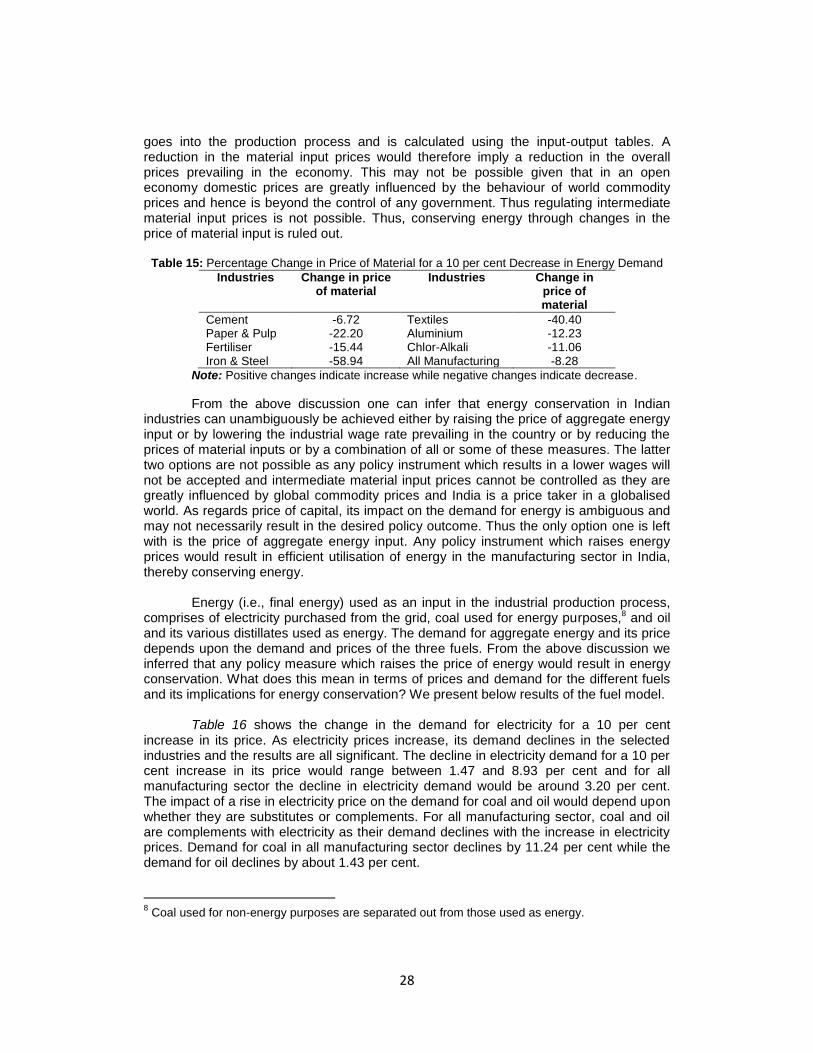
Table 15 shows the changes in material prices required for 10 per cent energy

conservation. In order to achieve the desired objective, material prices have to decline and rate of decline ranges between 6.72 and 40.40 per cent in the selected industries. Material input as defined in the study comprises of all non-energy intermediate inputs that

28

goes into the production process and is calculated using the input-output tables. A reduction in the material input prices would therefore imply a reduction in the overall prices prevailing in the economy. This may not be possible given that in an open economy domestic prices are greatly influenced by the behaviour of world commodity prices and hence is beyond the control of any government. Thus regulating intermediate material input prices is not possible. Thus, conserving energy through changes in the price of material input is ruled out.

Table 15: Percentage Change in Price of Material for a 10 per cent Decrease in Energy Demand

Industries Change in price of material

Industries Change in price of material

Cement -6.72 Textiles -40.40 Paper & Pulp -22.20 Aluminium -12.23 Fertiliser -15.44 Chlor-Alkali -11.06 Iron & Steel -58.94 All Manufacturing -8.28

Note: Positive changes indicate increase while negative changes indicate decrease.

From the above discussion one can infer that energy conservation in Indian industries can unambiguously be achieved either by raising the price of aggregate energy input or by lowering the industrial wage rate prevailing in the country or by reducing the prices of material inputs or by a combination of all or some of these measures. The latter two options are not possible as any policy instrument which results in a lower wages will not be accepted and intermediate material input prices cannot be controlled as they are greatly influenced by global commodity prices and India is a price taker in a globalised world. As regards price of capital, its impact on the demand for energy is ambiguous and may not necessarily result in the desired policy outcome. Thus the only option one is left with is the price of aggregate energy input. Any policy instrument which raises energy prices would result in efficient utilisation of energy in the manufacturing sector in India, thereby conserving energy.

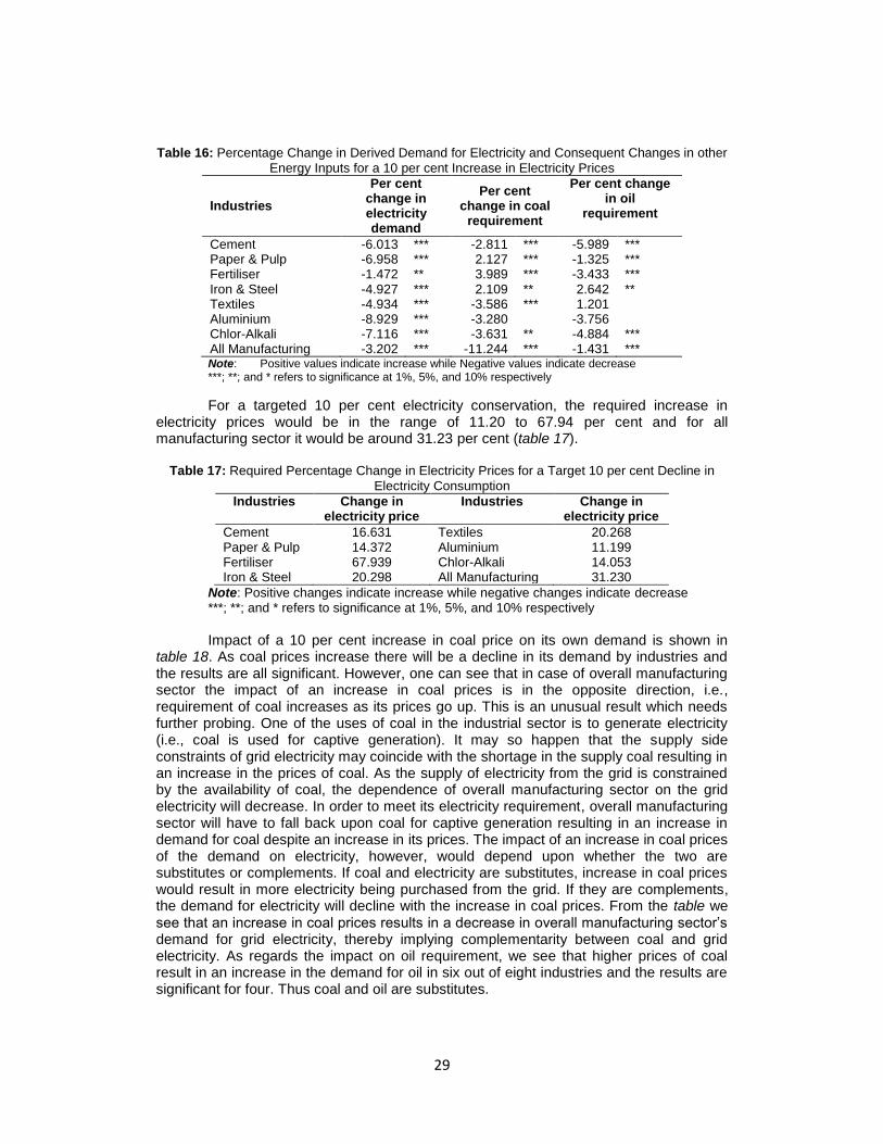
Energy (i.e., final energy) used as an input in the industrial production process, comprises of electricity purchased from the grid, coal used for energy purposes,8 and oil and its various distillates used as energy. The demand for aggregate energy and its price depends upon the demand and prices of the three fuels. From the above discussion we inferred that any policy measure which raises the price of energy would result in energy conservation. What does this mean in terms of prices and demand for the different fuels and its implications for energy conservation? We present below results of the fuel model. Table 16 shows the change in the demand for electricity for a 10 per cent increase in its price. As electricity prices increase, its demand declines in the selected industries and the results are all significant. The decline in electricity demand for a 10 per cent increase in its price would range between 1.47 and 8.93 per cent and for all manufacturing sector the decline in electricity demand would be around 3.20 per cent. The impact of a rise in electricity price on the demand for coal and oil would depend upon whether they are substitutes or complements. For all manufacturing sector, coal and oil are complements with electricity as their demand declines with the increase in electricity prices. Demand for coal in all manufacturing sector declines by 11.24 per cent while the demand for oil declines by about 1.43 per cent.

8 Coal used for non-energy purposes are separated out from those used as energy.

29

Table 16: Percentage Change in Derived Demand for Electricity and Consequent Changes in other

Energy Inputs for a 10 per cent Increase in Electricity Prices

Industries

Per cent change in electricity demand

Per cent change in coal

requirement

Per cent change in oil

requirement

Cement -6.013 *** -2.811 *** -5.989 *** Paper & Pulp -6.958 *** 2.127 *** -1.325 *** Fertiliser -1.472 ** 3.989 *** -3.433 *** Iron & Steel -4.927 *** 2.109 ** 2.642 ** Textiles -4.934 *** -3.586 *** 1.201 Aluminium -8.929 *** -3.280 -3.756 Chlor-Alkali -7.116 *** -3.631 ** -4.884 *** All Manufacturing -3.202 *** -11.244 *** -1.431 *** Note: Positive values indicate increase while Negative values indicate decrease ***; **; and * refers to significance at 1%, 5%, and 10% respectively

For a targeted 10 per cent electricity conservation, the required increase in electricity prices would be in the range of 11.20 to 67.94 per cent and for all manufacturing sector it would be around 31.23 per cent (table 17).

Table 17: Required Percentage Change in Electricity Prices for a Target 10 per cent Decline in

Electricity Consumption

Industries Change in electricity price

Industries Change in electricity price

Cement 16.631 Textiles 20.268 Paper & Pulp 14.372 Aluminium 11.199 Fertiliser 67.939 Chlor-Alkali 14.053 Iron & Steel 20.298 All Manufacturing 31.230

Note: Positive changes indicate increase while negative changes indicate decrease ***; **; and * refers to significance at 1%, 5%, and 10% respectively

Impact of a 10 per cent increase in coal price on its own demand is shown in

table 18. As coal prices increase there will be a decline in its demand by industries and the results are all significant. However, one can see that in case of overall manufacturing sector the impact of an increase in coal prices is in the opposite direction, i.e., requirement of coal increases as its prices go up. This is an unusual result which needs further probing. One of the uses of coal in the industrial sector is to generate electricity (i.e., coal is used for captive generation). It may so happen that the supply side constraints of grid electricity may coincide with the shortage in the supply coal resulting in an increase in the prices of coal. As the supply of electricity from the grid is constrained by the availability of coal, the dependence of overall manufacturing sector on the grid electricity will decrease. In order to meet its electricity requirement, overall manufacturing sector will have to fall back upon coal for captive generation resulting in an increase in demand for coal despite an increase in its prices. The impact of an increase in coal prices of the demand on electricity, however, would depend upon whether the two are substitutes or complements. If coal and electricity are substitutes, increase in coal prices would result in more electricity being purchased from the grid. If they are complements, the demand for electricity will decline with the increase in coal prices. From the table we see that an increase in coal prices results in a decrease in overall manufacturing sector’s demand for grid electricity, thereby implying complementarity between coal and grid electricity. As regards the impact on oil requirement, we see that higher prices of coal result in an increase in the demand for oil in six out of eight industries and the results are significant for four. Thus coal and oil are substitutes.

30

If one were to target a 10 per cent reduction in coal consumption, the required

increase in its price would be in the range of 5.66 to 11.73 per cent and in case of overall manufacturing sector the required increase in coal prices would be around 57.79 per cent (see, table 19).

Table 18: Percentage Change in Derived Demand for Coal & Consequent Changes in other

Energy Inputs for a 10 per cent Increase in Coal Prices

Industries Per cent

change in coal demand

Per cent change in electricity requirement

Per cent change in oil requirement

Cement -9.851 *** -3.535 *** 3.759 *** Paper & Pulp -8.821 *** 1.715 *** 0.957 *** Fertiliser -11.727 *** 2.139 *** 0.031 ** Iron & Steel -5.657 *** 0.802 * 0.495 Textiles -6.357 *** -0.435 *** 1.369 *** Aluminium -8.686 *** -1.415 0.512 Chlor-Alkali -7.963 *** -1.289 ** -0.310 All Manufacturing 1.730 *** -5.454 *** -0.205


Table 19: Required Percentage Change in Coal Prices for a Target 10 per cent Decline in Coal

Consumption

Industries Change in coal price

Industries Change in coal price

Cement 10.151 Textiles 15.731 Paper & Pulp 11.337 Aluminium 11.512 Fertiliser 8.527 Chlor-Alkali 12.558

Iron & Steel 17.678 All Manufacturing -57.792


Just as in case of electricity and coal, increase in the prices of oil also results in a

decline in its demand (table 20). The decrease in the demand for oil by industries is in the range of 4.20 to 9.40 per cent for a 10 percent increase in oil prices and these results are all found to be significant. If the objective of the government is to conserve oil consumption in the industrial sector, the prices of oil should increase. The price increase required for a 10 per cent reduction in oil consumption would be in the range of 10.64 to 23.82 per cent and for the all manufacturing sector the required increase would be 12.14 per cent (table 21).

Table 20: Percentage Change in Derived Demand for Oil and Consequent Changes in Other

Energy Inputs for a 10 per cent Increase in Oil Prices

Industries Per cent change in oil demand

Per cent change in electricity requirement

Per cent change in coal requirement

Cement -9.396 *** -2.078 *** 1.037 *** Paper & Pulp -5.640 *** -0.765 *** 0.686 *** Fertiliser -4.198 *** -8.268 *** 0.138 Iron & Steel -6.127 *** 1.135 ** 0.559 Textiles -7.394 *** 0.545 5.118 *** Aluminium -8.333 *** -1.233 0.390 Chlor-Alkali -7.094 *** -3.883 *** -0.694 All Manufacturing -8.236 *** -1.216 *** -0.359


31

Table 21: Required Percentage Change in Oil Prices for a Target 10 per cent Reduction in Oil

Consumption

Industries Change in oil price

Industries Change in oil price

Cement 10.643 Textiles 13.524 Paper & Pulp 17.730 Aluminium 12.000 Fertiliser 23.822 Chlor-Alkali 14.097 Iron & Steel 16.322 All Manufacturing 12.141


So far we looked at the impact of changes in prices of different fuels on their

respective demands and the demand for other fuels. But what is important from the point of view of energy conservation is the impact of changes in prices of different fuels on the demand for aggregate energy. If the price of electricity changes, not only will its own demand change, the demand for the other two fuels, i.e. coal and oil will also change thereby effecting the demand for aggregate energy. It is therefore, important to study the impact on the aggregate energy demand due to changes in prices of individual fuels. Table 22 shows the impact on the demand for aggregate energy due to a 10 per cent increase in the prices of different fuels. A 10 per cent increase in electricity prices would result in a decline in the demand for aggregate energy in the selected industries. The aggregate energy requirement would decline the least in iron and steel industry (around 1 per cent). The highest decline is observed in chlor-alkali industry (around 5.23 per cent). All manufacturing sector’s demand for energy will decline by around 3.84 per cent. Similarly increase in coal and oil prices by 10 per cent will also lead to a decline in aggregate energy requirement in the selected industries. For a 10 per cent increase in coal prices, the decline in aggregate energy demand would be in the range of 0.26 per cent (in iron and steel industry) to 6.82 per cent (in cement industry) and the energy demand in all manufacturing sector will decline of about 2.09 per cent. For oil, a 10 per cent increase in its price would result in a decline by aggregate energy demand in the range of 0.79 (in cement industry) to 4.69 per cent (in chlor-alkali industry) and for all manufacturing sector the decline in aggregate energy demand would be around 3.94 per cent.

Table 22: Per cent Change in Aggregate Energy Demand Due to a 10 per cent Increase in the

Price of Different Fuels

Industries Electricity Coal Oil

Cement -4.0162 -6.8156 -0.7939 Paper & Pulp -2.2343 -2.1826 -1.5911 Fertiliser -2.3643 -1.1356 -4.1004 Iron & Steel -0.9966 -0.2609 -1.7315 Textiles -3.0992 -0.7718 -0.9536 Aluminium -4.8081 -4.2089 -2.5600 Chlor-Alkali -5.2341 -2.4118 -4.6419 All Manufacturing -3.8365 -2.0916 -3.9443

Note: 1) Calculated on the basis of shares of different fuels prevailing in 2008-09 in the respective industry. However, for aluminium and chlor-alkali the shares are for the year 2007-08. 2) Positive changes indicate increase while negative changes indicate decrease.

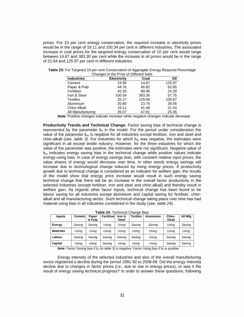
For a targeted 10 per cent reduction in aggregate energy consumption in each of the industries, table 23 shows the required change in prices of different fuels. Based on the industries’ derived demand for aggregate energy and different fuels, energy conservation will be associated with the rise in fuel and therefore aggregate energy

32

prices. For 10 per cent energy conservation, the required increase in electricity prices would be in the range of 19.11 and 100.34 per cent in different industries. The associated increase in coal prices for the targeted energy conservation of 10 per cent would range between 14.67 and 383.30 per cent while the increase in oil prices would be in the range of 21.54 and 125.97 per cent in different industries.

Table 23: For Targeted 10 per cent Conservation of Aggregate Energy Required Percentage

Changes in the Price of Different fuels

Industries Electricity Coal Oil

Cement 24.90 14.67 125.97 Paper & Pulp 44.76 45.82 62.85 Fertiliser 42.30 88.06 24.39 Iron & Steel 100.34 383.30 57.75 Textiles 32.27 129.58 104.87 Aluminium 20.80 23.76 39.06 Chlor-Alkali 19.11 41.46 21.54 All Manufacturing 26.07 47.81 25.35


Productivity Trends and Technical Change: Factor saving bias of technical change is represented by the parameter bit in the model. For the period under consideration the value of the parameter bet is negative for all industries except fertiliser, iron and steel and chlor-alkali (see, table 3). For industries for which bet was negative, the estimates were significant in all except textile industry. However, for the three industries for which the value of the parameter was positive, the estimates were not significant. Negative value of bet indicates energy saving bias in the technical change while positive values indicate energy using bias. In case of energy savings bias, with constant relative input prices, the value shares of energy would decrease over time. In other words energy savings will increase due to technological change induced by rising energy prices. If productivity growth due to technical change is considered as an indicator for welfare gain, the results of the model show that energy price increase would result in such energy saving technical change that there will be an increase in the overall factor productivity in the selected industries (except fertiliser, iron and steel and chlor-alkali) and thereby result in welfare gain. As regards other factor inputs, technical change has been found to be labour saving for all industries except aluminium and capital saving for fertiliser, chlor-alkali and all manufacturing sector. Such technical change taking place over time has had material using bias in all industries considered in the study (see, table 24).

Table 24: Technical Change Bias Inputs Cement Paper

& Pulp Fertiliser Iron &

Steel Textiles Aluminium Chlor-

Alkali All Mfg

Energy Saving Saving Using Using Saving Saving Using Saving

Materials Using Using Using Using Using Using Using Using

Labour Saving Saving Saving Saving Saving Using Saving Saving

Capital Using Using Saving Using Using Using Saving Saving

Note: Factor Saving bias if bit (in table 3) is negative; Factor Using bias if bit is positive

Energy intensity of the selected industries and also of the overall manufacturing sector registered a decline during the period 1991-92 to 2008-09. Did the energy intensity decline due to changes in factor prices (i.e., due to rise in energy prices), or was it the result of energy saving technical progress? In order to answer these questions, following

33

Sanstad et al. (2006),we define autonomous efficiency trend for the ith factor as

( )

and relate it to two familiar measures of technical change, namely,

(i) θit = ith factor price bias, defined as

, and

(ii) vt = rate of sectoral productivity, defined as - ( )

As suggested by Jorgenson and Hogan (1990) and Sanstad et al. (2006) one

can express the changes in sectoral productivity (vt) into two types of change (a) price

neutral technical change (

) and (b) factor price induced technical change ( ) as

(21)

From table 25 which shows the estimates of these changes derived using

parameter estimates of the factor model we see that the changes in factor productivity is mainly price induced (i.e., induced by increase in energy prices) and the results are all significant. The impact of changes which are price neutral can be in either direction and are not that important and are significant for some industries only. Thus we can infer that the changes in productivity in the selected industries are induced mainly by changes in factor (here energy) prices.

Table 25: Technical Change in Select Industries in India

(1991-92 to 2008-09)

Industry Productivity Price Neutral Price Induced

Cement 0.1242 -0.0723 *** 0.1965 *** Paper & Pulp 0.0659 -0.0118 *** 0.0777 *** Fertiliser 0.1049 0.0238 0.0812 ** Iron & Steel 0.1223 0.0095 0.1128 *** Textiles 0.0880 -0.0021 0.0901 *** Aluminium -0.3952 -0.0675 * -0.3277 *** Chlor-Alkali -0.9188 0.0026 -0.9214 *** All Manufacturing 0.1265 -0.0754 *** 0.2019 ***

6. Policy Conclusion

There exists considerable potential for energy savings in each of the seven

selected industries. However, the extent to which the energy savings potential can actually be achieved will depend on the existing technology of different units and economic viability of investments made to exploit such potential. In other words, will the gains from improving energy efficiency outweigh the costs of measures adopted to improve the energy efficiency? Nonetheless, efforts must be made to improve energy efficiency of all units within the industry so that improvement in the overall energy intensity of the industry can be achieved.

From the behavioural response of energy to changes in prices of inputs one can

conclude that reduction in energy consumption in the industrial sector can be achieved by raising the price of aggregate energy input. For a target 10 per cent reduction in energy consumption the required increase in energy prices would be in the range of 8.14 to 33.46 per cent. Any policy or economic instrument which raises the price of energy input

34

would result in energy conservation by improving the energy efficiency of the industrial sector. A tax on the consumption of energy is one such instrument which would yield the desired outcome. Aggregate energy consumed by the industries comprises of three fuels, electricity purchased from the grid, coal used as energy, and oil and oil products used as energy. The results of the model indicate that an increase in price of these fuels would not only result in a decline in their own consumption but also in the consumption of aggregate energy. Thus, energy conservation in the industrial sector can be achieved by raising the prices of individual fuels.

A tax, either specific or ad valorem, levied by the government on the

consumption of different fuels would raise the price of fuels consumed by the industrial sector. This will raise the cost of production of the industrial sector thereby affecting the quantity of inputs including energy inputs consumed. The demand for energy inputs will decline as the industry will be forced to move towards efficient utilisation of energy. Thus, a tax levied by the central government on individual fuels would result in energy conservation. However, the proposed tax should conform to the norms of the present tax system in the country.

India has introduced the value added tax (VAT) and is in the process of moving

towards a comprehensive system of value added tax under the name of Goods and Services Tax (GST). In near future as GST will be implemented, any new tax proposed should conform to the norms of GST. Any tax levied by the Central Government on the consumption of different fuels would have the desired effect of energy conservation provided the user of energy in the production chain cannot pass on the burden to the consumer of the products without facing any rise in the cost of production. In a VAT or GST regime, producers earn input tax credit on the taxes on different inputs paid by them. The net tax liability of a producer would be the difference between his/her total tax liability and the taxes paid by him/her on the inputs used in the production process. In such a case imposing a tax on fuels which are used as inputs will not yield desired results as the taxes paid on energy inputs by the producers would be credited back to them and would not therefore, be reflected in their cost of production. In order to overcome this problem, it is proposed that the Central Government levy a non-rebatable excise duty on fuels and energy over and above the normal GST. Such an excise duty can be in the form of a specific duty or an ad valorem duty on the consumption of different fuels. This non-rebatable excise duty should also have a countervailing component for fuel inputs which are imported. Such non-rebatable excise duty on energy inputs like electricity, coal, and oil would work through the production structure and affect the prices of goods that use the energy inputs thereby affecting the competitiveness of the manufacturing units. Units which consume more energy per unit of output will have a relatively higher cost of production as their tax liability on account of higher energy consumption will be higher vis-à-vis units which have relatively lower energy intensity. This would adversely affect the profitability and competitiveness of these units thereby forcing them to either utilise energy efficiently or undergo technological restructuring through modernisation for switching to an altogether new and more energy efficient production process.

35

References

Apte P.C., 1983. “Substitution among Energy and Non-Energy Inputs in Selected Indian Manufacturing Industries: An Economic Analysis,” Indian Economic Journal, 31(2); 71-90.

Berndt, Ernst R. and David O. Wood, 1975. Technology, Prices, and the Derived

Demand for Energy, Review of Economics and Statistics, 57(3); 259-268. Field, B.C. and C. Grebenstien, 1980. “Capital-Energy Substitution in U.S.

Manufacturing,” Review of Economics and Statistics, 62(2); 207-212 Fuss M.A., 1977. “The Demand for Energy in Canadian Manufacturing: An Example of

the Estimation of Production Structures with many Inputs”, Journal of Econometrics, 5; 89-116.

Government of India (GoI), 2008. Input-Output Tables 2003-04, Ministry of Statistics and

Programme Implementation, New Delhi. ---------, (various years), Annual Survey of Industries, Ministry of Statistics and

Programme Implementation, New Delhi. ----------, (various years), Energy Statistics, National Statistical Organisation, Ministry of

Statistics and Programme Implementation, New Delhi. ----------, (various years), Petroleum and Natural Gas Statistics, Economic Division,

Ministry of Petroleum and Natural Gas, New Delhi. Griffin J.M., 1977. “Inter-Fuel Substitution Possibilities: A Translog Application to Inter-

country Data”, International Economic Review, 18(3); 755-770. Griffin J.M. and P.R. Gregory, 1976. “An Intercountry Translog Model of Energy

Substitution Responses,” American Economic Review, 66(5); 845-857. Halvorsen, R., 1977. “Energy Substitution in U.S. Manufacturing”, Review of Economics

and Statistics, 59(4); 381-388. Hogan William W. and Dale Jorgenson, 1991. “Productivity Trends and the Cost of

Reducing CO2 Emissions,” The Energy Journal, 12(1); 67-85. Hudson E.A. and D.W. Jorgenson, 1974. “U.S. Energy Policy and Economic Growth,

1975-2000,” Bell Journal of Economics and Management Science, 5(2); 461-514.

Jha R., M.N. Murty, S. Paul, and B.B. Rao, 1993. An Analysis of Technical Change,

Factor Substitution and Economies of Scale in Manufacturing Industries in India, Applied Economics, 25; 1337-1343.

36

Kar J. and D. Chakraborty, 1986. “Interfuel Substitution Possibilities in Indian Manufacturing Industries – A Translog Approach,” Artha Vijnana, 28(2); 133-151.

Magnus Jan R., 1979. “Substitution between Energy and Non-Energy Inputs in the

Netherlands 1950-1976,” International Economic Review, 20(2); 465-484. Murty M.N., 1986. “Interfuel Substitution and Derived Demands for Inputs in the

Manufacturing Sector of India,” Journal of Quantitative Economics, 2(1); 119-135.

Ozatalay, S., S. Grubaugh, and T.V. Long, 1979. “Energy Substitution and National

Energy Policy,” American Economic Review, 69(2); 369-371. Pindyck, R.S., 1979. “Interfuel Substitution and the Industrial Demand for Energy: An

International Comparison”, Review of Economics and Statistics, 61(2); 169-179. Pitt Mark M., 1985. “Estimating Industrial Energy Demand with Firm-Level Data: The

Case of Indonesia,” The Energy Journal, 6(2); 25-39. Roy, J., A. Sanstad, J.A. Sathaye and R. Khaddaria, 2006. “Substitution and price

elasticity estimates using inter-country pooled data in a translog cost model”, Energy Economics, 28; 706-719.

Roy, J., J. Sathaye, A. Sanstad, P. Mongia, and K. Schumacher, 1999. “Productivity

Trends in India's Energy-Intensive Industries”, Energy Journal, 20(3); 33-61. Roy Joyashree, 1992. Demand for Energy in Indian Industries: A Quantitative Approach,

Delhi 110006 : Daya Publishing House. Saha Anindita Roy, 1997. The Economics of Energy Conservation and Industrial

Cogeneration of Electricity: Case Studies of Certain Selected Industries in India. Unpublished Ph.D. Thesis submitted to the Jawaharlal Nehru University.

Sanstad A.H., J. Roy, and J.A. Sathaye, 2006. “Estimating Energy-Augmenting

Technological Change in Developing Country Industries,” Energy Economics, 28; 720–729.

Uri N.D., 1979. “Energy Demand and Inter-fuel Substitution India,” European Economic

Review, 12;181-190. Williams M. and P. Laumas, 1981. “The Relation between Energy and Non-Energy Inputs

in India's Manufacturing Industries”, Journal of Industrial Economics, 30(2);113-122.

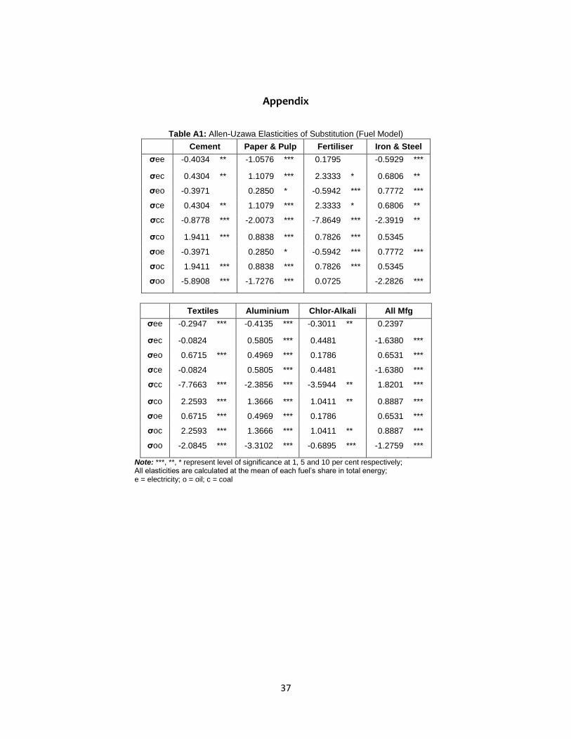
37

Appendix

Table A1: Allen-Uzawa Elasticities of Substitution (Fuel Model)


σee -0.4034 ** -1.0576 *** 0.1795 -0.5929 ***

σec 0.4304 ** 1.1079 *** 2.3333 * 0.6806 **

σeo -0.3971 0.2850 * -0.5942 *** 0.7772 ***

σce 0.4304 ** 1.1079 *** 2.3333 * 0.6806 **

σcc -0.8778 *** -2.0073 *** -7.8649 *** -2.3919 **

σco 1.9411 *** 0.8838 *** 0.7826 *** 0.5345

σoe -0.3971 0.2850 * -0.5942 *** 0.7772 ***

σoc 1.9411 *** 0.8838 *** 0.7826 *** 0.5345

σoo -5.8908 *** -1.7276 *** 0.0725 -2.2826 ***


σee -0.2947 *** -0.4135 *** -0.3011 ** 0.2397

σec -0.0824 0.5805 *** 0.4481 -1.6380 ***

σeo 0.6715 *** 0.4969 *** 0.1786 0.6531 ***

σce -0.0824 0.5805 *** 0.4481 -1.6380 ***

σcc -7.7663 *** -2.3856 *** -3.5944 ** 1.8201 ***

σco 2.2593 *** 1.3666 *** 1.0411 ** 0.8887 ***

σoe 0.6715 *** 0.4969 *** 0.1786 0.6531 ***

σoc 2.2593 *** 1.3666 *** 1.0411 ** 0.8887 ***

σoo -2.0845 *** -3.3102 *** -0.6895 *** -1.2759 ***

Note: ***, **, * represent level of significance at 1, 5 and 10 per cent respectively; All elasticities are calculated at the mean of each fuel’s share in total energy; e = electricity; o = oil; c = coal

38

Table A2: Own and Cross Partial Price Elasticities (Fuel Model)


ηee -0.1549 ** -0.4437 *** 0.0455 -0.3275 ***

ηec 0.2078 ** 0.3747 *** 0.3172 * 0.1431 **

ηeo -0.0529 0.0690 * -0.3627 *** 0.1845 ***

ηce 0.1653 ** 0.4648 *** 0.5916 * 0.3760 **

ηcc -0.4238 *** -0.6789 *** -1.0694 *** -0.5028 **

ηco 0.2586 *** 0.2141 *** 0.4778 *** 0.1269

ηoe -0.1525 0.1196 * -0.1506 *** 0.4294 ***

ηoc 0.9372 *** 0.2989 *** 0.1064 *** 0.1124

ηoo -0.7847 *** -0.4185 *** 0.0442 -0.5417 ***


ηee -0.1871 *** -0.2350 *** -0.1400 0.1026

ηec -0.0063 0.1423 *** 0.0740 -0.3403 ***

ηeo 0.1934 *** 0.0927 *** 0.0661 0.2377 ***

ηce -0.0523 0.3299 *** 0.2084 -0.7016 ***

ηcc -0.5985 *** -0.5848 *** -0.5934 ** 0.3781 ***

ηco 0.6508 *** 0.2549 *** 0.3850 ** 0.3234 ***

ηoe 0.4263 *** 0.2824 *** 0.0831 0.2797 ***

ηoc 0.1741 *** 0.3350 *** 0.1719 ** 0.1846 ***

ηoo -0.6005 *** -0.6174 *** -0.2550 *** -0.4643 ***

Note: ***, **, * represent level of significance at 1, 5 and 10 per cent respectively; All elasticities are calculated at the mean of each fuel’s share in total energy; e = electricity; o = oil; c = coal

39

Table A3: Allen-Uzawa Elasticities of Substitution (Factor Model)


σll -3.1022 -6.9736 *** -5.7161 *** -2.3228

σlk -1.3056 * 0.4190 -0.0510 -1.0207 **

σle 2.1453 *** 1.9840 *** -0.3965 4.2994 ***

σlm -0.3015 0.1238 0.3908 ** -0.2714 *

σkl -1.3056 * 0.4190 -0.0510 -1.0207 **

σkk 2.5035 * -2.7181 * -4.1271 *** -1.6748 **

σke -2.3860 *** 0.1868 0.9702 -0.6533

σkm 0.3511 0.5395 0.6066 *** 0.4583 ***

σel 2.1453 *** 1.9840 *** -0.3965 4.2994 ***

σek -2.3860 *** 0.1868 0.9702 -0.6533

σee -4.8519 *** -4.1118 *** -6.4908 *** -2.9187

σem 2.7146 *** 0.6990 *** 0.9101 ** 0.2353

σml -0.3015 0.1238 0.3908 ** -0.2714 *

σmk 0.3511 0.5395 0.6066 *** 0.4583 ***

σme 2.7146 *** 0.6990 *** 0.9101 ** 0.2353

σmm -1.2750 *** -0.2939 *** -0.2836 *** -0.0957 ***


σll -7.2852 *** -4.7318 -3.0663 1.4168

σlk -0.0034 1.6630 * 0.1540 -2.5892 ***

σle 4.1251 *** 5.0755 * -1.3581 4.1532 ***

σlm 0.2970 ** -1.1660 * 0.5704 * -0.0629

σkl -0.0034 1.6630 * 0.1540 -2.5892 ***

σkk -5.2489 ** -1.3874 -5.7424 *** -2.9221 **

σke -0.8083 0.6662 2.7321 *** -3.9479 ***

σkm 0.8917 *** 0.0049 0.6622 * 0.9204 ***

σel 4.1251 *** 5.0755 * -1.3581 4.1532 ***

σek -0.8083 0.6662 2.7321 *** -3.9479 ***

σee -5.5792 *** -7.5331 ** -8.0492 *** -15.6470 ***

σem 0.3413 * 1.2353 1.4122 ** 1.5626 ***

σml 0.2970 ** -1.1660 * 0.5704 * -0.0629

σmk 0.8917 *** 0.0049 0.6622 * 0.9204 ***

σme 0.3413 * 1.2353 1.4122 ** 1.5626 ***

σmm -0.2079 *** -0.2011 -0.5422 *** -0.2559 *** Note: 1) ***, **, * represent level of significance at 1, 5 and 10 per cent respectively; 2) All elasticities are calculated at the mean of each factor share; 3) l = labour; e = energy; k = capital; m = intermediate material input

Documents

Energy Savings Potential and Policy for Energy ... · PDF fileEnergy Savings Potential and Policy for Energy Conservation in Selected Indian Manufacturing Industries Manish Gupta and