Energy preserving methods for nonlinear Schrödinger equations

HAL Id: hal-01951527https://hal.archives-ouvertes.fr/hal-01951527

Submitted on 11 Dec 2018

HAL is a multi-disciplinary open accessarchive for the deposit and dissemination of sci-entific research documents, whether they are pub-lished or not. The documents may come fromteaching and research institutions in France orabroad, or from public or private research centers.

L’archive ouverte pluridisciplinaire HAL, estdestinée au dépôt et à la diffusion de documentsscientifiques de niveau recherche, publiés ou non,émanant des établissements d’enseignement et derecherche français ou étrangers, des laboratoirespublics ou privés.

Energy preserving methods for nonlinear Schrödingerequations

Christophe Besse, Stephane Descombes, Guillaume Dujardin, IngridLacroix-Violet

To cite this version:Christophe Besse, Stephane Descombes, Guillaume Dujardin, Ingrid Lacroix-Violet. Energy pre-serving methods for nonlinear Schrödinger equations. IMA Journal of Numerical Analysis, OxfordUniversity Press (OUP), 2021, 41 (1), pp.618-653. 10.1093/imanum/drz067. hal-01951527

https://hal.archives-ouvertes.fr/hal-01951527

https://hal.archives-ouvertes.fr

ENERGY PRESERVING METHODS FOR NONLINEAR SCHRODINGER

EQUATIONS

CHRISTOPHE BESSE, STEPHANE DESCOMBES, GUILLAUME DUJARDIN,AND INGRID LACROIX-VIOLET

Abstract. This paper is concerned with the numerical integration in time of nonlinearSchrodinger equations using different methods preserving the energy or a discrete analog ofit. The Crank-Nicolson method is a well known method of order 2 but is fully implicit andone may prefer a linearly implicit method like the relaxation method introduced in [10] forthe cubic nonlinear Schrodinger equation. This method is also an energy preserving methodand numerical simulations have shown that its order is 2. In this paper we give a rigorousproof of the order of this relaxation method and propose a generalized version that allowsto deal with general power law nonlinearites. Numerical simulations for different physicalmodels show the efficiency of these methods.

AMS Classification: 35Q41, 81Q05, 65M70

Keywords. Nonlinear Schrodinger equation, Gross-Pitaevskii equation, numerical methods, relax-ation methods.

1. Introduction

The nonlinear Schrodinger equation (NLSE) is a fairly general dispersive partial differential equationarising in many areas of physics and chemistry [1, 2, 16, 23, 12]. One of the most important applicationof the NLSE is for laser beam propagation in nonlinear and/or quantum optics and there it is alsoknown as parabolic/paraxial approximation of the Helmholtz or time-independent Maxwell equations[1, 2, 16, 12]. In the context of the modeling of the Bose-Einstein condensation (BEC), the nonlinearSchrodinger equation is known as the Gross-Pitaevskii equation (GPE), which is a widespread modelthat describes the averaged dynamics of the condensate [23, 6]. Depending on the physical situationthat one considers, several terms in the right-hand side of the NLSE appear. Our goal is to developnumerical methods for the time integration of a fairly general NLSE including realistic physical situa-tions, that have high-order in time and have good qualitative properties (preservation of mass, energy,etc) over finite times. We develop our analysis in spatial dimension d P t1, 2, 3u because it fits thephysical framework, even if most methods and results naturally extend to higher dimensions. Thespace variable x will sometimes lie in Rd, sometimes on the d-dimensional torus Tdδ “ pRpδZqqd (forsome δ ą 0). In this paper, we consider a NLSE of the form

(1) iBtϕpt, xq “

ˆ

´1

2∆` V pxq ` β|ϕ|2σpt, xq ` λ

`

U ˚ |ϕpt, ¨q|2˘

pxq ´ Ω.R

˙

ϕpt, xq,

where ϕ is an unknown function from R ˆ Rd or R ˆ Tdδ to C, ∆ is the Laplace operator, V is somereal-valued potential function, β P R is a parameter that measures the local nonlinearity strength,λ P R is a parameter that measures the nonlocal nonlinearity strength with convolution kernel U ,Ω P Rd is a vector encoding the direction and the speed of a rotation, and R is a rotation operatorthat is important in the modeling of rotating BEC (for example, R “ x ^ pí∇q when d “ 3). TheNLSE is supplemented with an initial datum ϕin. The results presented in this paper extend to more

1

2 C. BESSE, S. DESCOMBES, G. DUJARDIN, AND I. LACROIX-VIOLET

general power law nonlinearities such as

iBtϕpt, xq “

˜

´1

2∆` V pxq `

Kÿ

k“1

βk|ϕ|2σkpt, xq ` λ

`

U ˚ |ϕpt, ¨q|2˘

pxq ´ Ω.R

¸

ϕpt, xq,

but we restrict ourselves to K “ 1 for the sake of simplicity. Equation (1) is hamiltonian for the energyfunctional

(2) Epϕq “

ż

Rd

ˆ

1

4∇ϕ2 ` 1

2V |ϕ|2 `

β

2σ ` 2|ϕ|2σ`2 `

λ

4pU ˚ |ϕ|2q|ϕ|2 ´

Ω

2ϕRϕ

˙

dx,

provided U is a real-valued convolution kernel, symmetric with respect to the origin 1. In practicethe convolution kernel U may for example correspond to a Poisson equation (Upxq “ 1p4π|x|q indimension d “ 3) or it may represent dipole-dipole interactions (see [9]).

The main goal of this paper is the analysis of numerical methods for the time integration of (1) thatpreserve the energy (2) or a discretized analogue of it. In particular, we are interested in the order(in time) of such methods. A well known method is the Crank-Nicolson method introduced in [14] forparabolic problems (see for example a posteriori error estimates in [3]) and applied in [17] to Schro-dinger equations. For all nonlinearities, these methods are fully implicit. However, they have secondorder in time (see [24] for the case of the cubic NLS equation and [28] for the case of a system withpossibly fractional derivatives) and preserve discrete analogues of the energy (2) as well as the totalmass (squared L2-norm) of the solutions. Unfortunately, since they are fully implicit, these methodsare costly. To work around this problem, the methods introduced and analyzed in this paper belongto the family of relaxation methods.

Relaxation methods for Schrodinger equations were introduced in [10, 11]. They have been appliedto different NLS equation for example in the context of plasma physics [22]. For cubic nonlinearities(σ “ 1 in (1)), they are linearly implicit hence very popular [4, 15, 6, 18, 20]. They preserve theL2-norm and a discrete analogue of (2). It is well-known that they have numerical order 2 but up toour knowledge there is no proof of order 2 in the literature. This paper presents two new results withrespect to relaxation methods for (1). First, we prove rigorously that the classical relaxation method,applied to the classical cubic NLS equation (i.e. (1) with V ” 0, β “ 1, σ “ 1, λ “ 0 and Ω “ 0) is oforder 2. Second, we present a generalized relaxation method that allows to deal with general powerlaw nonlinearities (σ ‰ 1 in (1)) and with the full GPE. The generalized relaxation methods that weintroduce in this context are implicit (actually explicit for σ ď 4), have numerical order 2 and we showthat they preserve an energy which is also a discretized analogue of (2).

This paper is organized as follows. In Section 2 we recall the definition of the Crank-Nicolson methodand give a short explanation of its energy preserving property. Section 3 is devoted to relaxationmethods applied to (1): In a first part we recall the method introduced in [10] for the cubic Schrodingerequation and in a second part we give a proof of the optimal order of convergence for an initial datumbelonging to Hs`4pRdq, d in t1, 2, 3u and s ą d2. In section 4 we propose a generalized relaxationmethod that allows to deal with general nonlinearites and we prove that this method is also an energypreserving method. Section 5 deals with numerical results in different physical models showing theefficiency of the methods.

2. Preservation of energy and Crank-Nicolson scheme

A usual way to prove the conservation of the energy (2) consists in multiplying the equation (1) byBtϕpt, xq, where z denotes the conjugate value of a complex z, integrating over Rd and taking the realpart of the result. This computation relies on the identity which holds for all smooth functions ϕ of

1For real-valued functions, symmetry with respect to the origin is equivalent to real-valued Fouriertransform.

ENERGY PRESERVING METHODS FOR NLSE 3

time with values into a space of sufficiently integrable functions

(3) Re

ż

Rd|ϕ|2σϕBtϕdx “

1

2σ ` 2

d

dt

ż

Rd|ϕ|2σ`2 dx, @σ ě 0.

A possible way to derive numerical schemes that preserve an energy functional is therefore to mimicthis identity at the discrete level.

In 1981, Delfour, Fortin and Payre [17], following an idea of Strauss and Vasquez [26], proposed away to deal with the nonlinear term |ϕ|2σϕ for the Crank-Nicolson scheme. This method generalizesthe second order mid-point scheme for the linear Schrodinger equation

iϕn`1 ´ ϕn

δt“ ´

1

2∆ϕn`1 ` ϕn

2,

where ϕnpxq denotes an approximation of ϕptn, xq with the discrete time tn “ nδt defined with thetime step δt. Their approach can be explained as follows. If one looks for a real-valued functiong : C2 Ñ R such that the scheme takes the form

(4) iϕn`1 ´ ϕn

δt“

ˆ

´1

2∆` V ` βgpϕn, ϕn`1q ` λ

ˆ

U ˚

ˆ

|ϕn`1|2 ` |ϕn|

2

2

˙˙

´ Ω.R

˙

ϕn`1 ` ϕn2

,

then, multiplying this relation by iϕn`1 ´ ϕn, integrating overs Rd and taking the real part, as wedid in the time-continuous setting above, yields to 0 in the left-hand side and several terms in theright-hand side. Amongst these terms, those involving g are equal to

β

ż

Rdgpϕn, ϕn`1q

`

|ϕn`1|2 ´ |ϕn|

2˘

dx,

since g is real-valued. Let us denote by G the function v ÞÑ |v|2σ`2p2σ ` 2q. A sufficient conditionfor the method (4) to preserve an energy of the form (2) is therefore to have

gpϕn, ϕn`1q`

|ϕn`1|2 ´ |ϕn|

2˘

“ Gpϕn`1q ´Gpϕnq.

This is exactly the definition of g chosen in [17].In the following, the Crank-Nicolson method for the GPE (1) is therefore defined using the formula

iϕn`1 ´ ϕn

δt(5)

“

ˆ

´1

2∆` V `

β

σ ` 1

|ϕn`1|2σ`2 ´ |ϕn|

2σ`2

|ϕn`1|2 ´ |ϕn|2

` λ

ˆ

U ˚

ˆ

|ϕn`1|2 ` |ϕn|

2

2

˙˙

´ Ω.R

˙

ϕn`1 ` ϕn2

.

We shall use the notation

ϕn`1 “ ΦCNδt pϕnq,

for the Crank-Nicolson method (5). In the expression above, the term corresponding to the nonlinearityshould be understood as

(6)β

σ ` 1

|ϕn`1|2σ`2 ´ |ϕn|

2σ`2

|ϕn`1|2 ´ |ϕn|2

“β

σ ` 1

σÿ

k“0

|ϕn`1|2k|ϕn|

2pσ´kq,

so that it is indeed non-singular and it is consistent with the non-linear term β|ϕ|2σ. The Crank-Nicolson method is fully implicit. It is known to have order two for the cubic NLS equation [24].Moreover it preserves exactly the L2-norm of the solution as well as the following energy:

(7) ECNpϕq “ Epϕq,

with E defined by (2).In Section 4, we shall use similar ideas to derive energy-preserving relaxation methods for general

power laws nonlinearities. Before doing so, we first deal with the classical relaxation method in Section3.


3. The classical relaxation method

3.1. An energy preserving method. In [11], Besse introduced the usual relaxation method (10)applied to the nonlinear Schrodinger equation (1) with V “ 0, λ “ 0, Ω “ 0 and σ “ 1 that is knownas the cubic nonlinear Schrodigner equation

(8) iBtϕpt, xq “ ´1

2∆ϕpt, xq ` β|ϕpt, xq|2ϕpt, xq,

with ϕp0, xq “ ϕinpxq. The idea of the relaxation method is to add to (8) a new unknown Υ “ |ϕ|2

and the equation (8) is transformed in

(9)

#

Υ “ |ϕpt, xq|2,

iBtϕpt, xq “ ´1

2∆ϕpt, xq ` βΥϕpt, xq.

The relaxation method then consists in discretizing both equations respectively at discrete times tnand tn`12 and to solve iteratively

(10)

$

’

&

’

%

Υn`12 `Υn´12

2“ |ϕn|

2,

iϕn`1 ´ ϕn

δt“

ˆ

´1

2∆` βΥn`12

˙

ϕn`1 ` ϕn2

,

to compute approximations ϕn of ϕpnδtq. This system is usually initialized with Υ´12 “ |ϕp´δt2q|2

or by second order approximation of |ϕp´δt2q|2. This method is linearly implicit (recall that σ “ 1).Moreover, it is known to preserve exactly the L2-norm and the discrete energy [11]:

(11) Erlxpϕ,Υq “1

4

ż

Rd∇ϕ2dx` β

2

ż

RdΥ|ϕ|2dx´

β

4

ż

RdΥ2dx.

Indeed

Re

ˆ

Υn`12ϕn`1 ` ϕn

2ϕn`1 ´ ϕn

˙

“Υn`12

2

´

|ϕn`1|2 ´ |ϕn|

2¯

.

But

Υn`12

´

|ϕn`1|2 ´ |ϕn|

2¯

“ Υn`12

´

|ϕn`1|2 ´ |ϕn|

2¯

`Υn´12

´

|ϕn|2 ´ |ϕn|

2¯

“

´

Υn`12|ϕn`1|2 ´Υn´12|ϕn|

2¯

´

´

Υn`12 ´Υn´12

¯

|ϕn|2.

Using the definition of Υ¨`12 in (10), a simple computation leads to

´

Υn`12 ´Υn´12

¯

|ϕn|2 “

´

Υn`12

¯2

´

´

Υn´12

¯2

2.

We therefore conclude that

Re

ˆ

Υn`12ϕn`1 ` ϕn

2ϕn`1 ´ ϕn

˙

“

´

Υn`12|ϕn`1|2 ´Υn´12|ϕn|

2¯

`

´

Υn`12

¯2

´

´

Υn´12

¯2

2,

which allows to prove the conservation of the discrete energy (11).It is interesting to note the consistency of the energy associated to relaxation scheme with the

energy (2) for cubic nonlinear Schrodinger equation

Erlxpϕ, |ϕ|2q “ Epϕq.

The relaxation method was proved to converge in [11] but consistency analysis was missing. We presentit in the next subsection.


3.2. Consistency analysis for NLS equation with cubic nonlinearity. The aim of this subsec-tion is to prove that this method has temporal order 2 under fairly general assumptions. This factis supported by numerical evidences in the literature for years. We provide the first rigorous proofbelow.

The first equation in (10) is the discrete equivalent of the continuous constraint Υ “ |ϕ|2. Inparticular, this constraint is not an evolution equation. Therefore, we use the ideas introduced in [11]and rewrite the continuous equation (1) (recall that V “ 0, λ “ 0 and Ω “ 0 and σ “ 1) as the system

(12)

$

’

’

&

’

’

%

iBtϕ`1

2∆ϕ “ βΥϕ,

BtΥ “ 2Repvϕq,

iBtv `1

2∆v “ βpBtΥϕ`ΥBtϕq.

The discrete system (10) has a discrete augmented equivalent (see [10, 11]). Let us denote by vn` 12“

ϕn`1 ´ ϕnδt

the discrete time derivative of ϕn and define the nonlinearities as

(13)

$

’

’

’

’

’

’

’

’

’

’

&

’

’

’

’

’

’

’

’

’

’

%

Φn` 12“ Υn` 1

2

ˆ

ϕn`1 ` ϕn2

˙

,

Ξn` 12“ 2Re

ˆ

vn` 12

ˆ

ϕn`1 ` ϕn2

˙˙

,

Vn` 12“

ˆ

Υn` 32`Υn´ 1

2

2

˙ˆ

vn` 32` 2vn` 1

2` vn´ 1

2

4

˙

`2Re

ˆ

vn` 12

ˆ

ϕn`1 ` ϕn2

˙˙ˆ

ϕn`2 ` ϕn`1 ` ϕn ` ϕn´1

4

˙

.

The augmented system writes

(14)

$

’

’

’

’

’

’

’

&

’

’

’

’

’

’

’

%

iϕn`2 ´ ϕn`1

δt`

1

2∆

ˆ

ϕn`2 ` ϕn`1

2

˙

“ βΦn` 32, p14.bq

Υn` 32´Υn´ 1

2

2δt“ Ξn` 1

2, p14.aq

ivn` 3

2´ vn´ 1

2

2δt`

1

2∆

ˆ

vn` 32` 2vn` 1

2` vn´ 1

2

4

˙

“ βVn` 12. p14.cq

This system allows to compute pϕn`2,Υn` 32, vn` 3

2q from

Xn :“´

Υn´ 12,Υn` 1

2, ϕn´1, ϕn, ϕn`1, vn´ 1

2, vn` 1

2

¯

.

We consider the system (14) as the mapping

Xn ÞÑ Xn`1.

The seven variables involved in Xn are not independent. If they satisfiy the five relations

$

’

’

’

’

’

’

’

’

’

’

&

’

’

’

’

’

’

’

’

’

’

%

vn´ 12“ϕn ´ ϕn´1

δt,

vn` 12“ϕn`1 ´ ϕn

δt,

Υn` 12`Υn´ 1

2“ 2|ϕn|

2,

iϕn ´ ϕn´1

δt“

ˆ

´1

2∆` βΥn´12

˙

ϕn ` ϕn´1

2,

iϕn`1 ´ ϕn

δt“

ˆ

´1

2∆` βΥn`12

˙

ϕn`1 ` ϕn2

,


then the seven variables in Xn`1 satisfy the same five relations with n replaced by n` 1. This fact isproved in [11]. We describe now how to build the seven initial data in X0 from ϕ0 “ ϕin and Υ´ 1

2so

that they satisfy the five relations above:

(15)

$

’

’

’

’

’

’

’

’

’

&

’

’

’

’

’

’

’

’

’

%

Υ 12

“ 2|ϕ0|2 ´Υ´ 1

2,

ϕ´1 “

ˆ

2´ iδt

ˆ

´1

2∆` βΥ´12

˙˙´1ˆ

2` iδt

ˆ

´1

2∆` βΥ´12

˙˙

ϕ0,

ϕ1 “

ˆ

2` iδt

ˆ

´1

2∆` βΥ12

˙˙´1ˆ

2´ iδt

ˆ

´1

2∆` βΥ12

˙˙

ϕ0,

v´ 12“ pϕ0 ´ ϕ´1qδt,

v 12

“ pϕ1 ´ ϕ0qδt.

Let us define the operators

A “ pi´ δt∆4q´1pi` δt∆4q and B “ pi´ δt∆4q´1,

and the matrix of operators

C “

¨

˚

˚

˚

˚

˚

˚

˚

˚

˝

I 0 0 0 0 0 00 I 0 0 0 0 00 0 B 0 0 0 00 0 0 B 0 0 00 0 0 0 B 0 00 0 0 0 0 B 00 0 0 0 0 0 B

˛

‹

‹

‹

‹

‹

‹

‹

‹

‚

.

The mapping Xn ÞÑ Xn`1 reads

(16)

¨

˚

˚

˚

˚

˚

˚

˚

˚

˚

˝

Υn` 12

Υn` 32

ϕnϕn`1

ϕn`2

vn` 12

vn` 32

˛

‹

‹

‹

‹

‹

‹

‹

‹

‹

‚

“

¨

˚

˚

˚

˚

˚

˚

˚

˚

˝

0 I 0 0 0 0 0I 0 0 0 0 0 00 0 0 I 0 0 00 0 0 0 I 0 00 0 0 0 A 0 00 0 0 0 0 0 I0 0 0 0 0 A A´ I

˛

‹

‹

‹

‹

‹

‹

‹

‹

‚

¨

˚

˚

˚

˚

˚

˚

˚

˚

˚

˝

Υn´ 12

Υn` 12

ϕn´1

ϕnϕn`1

vn´ 12

vn` 12

˛

‹

‹

‹

‹

‹

‹

‹

‹

‹

‚

` δtC

¨

˚

˚

˚

˚

˚

˚

˚

˚

˝

02Ξn` 1

2

00

βΦn` 32

02βVn` 1

2

˛

‹

‹

‹

‹

‹

‹

‹

‹

‚

.

In a more compact form, we define B and M so that the mapping (16) reads

(17) Xn`1 “ BXn ` δtCMpXn, Xn`1q.

We introduce the hypotheses that will allow us to prove our consistency and convergence result forthe classical relaxation method (10) in Theorem 8.

Remark 1. The results below extend to more general cases. In particular, one may treat the casewhere V is non zero smooth autonomous potential such that the multiplication by V is a bounded linearoperator between Sobolev spaces and the case where V is a nonautonomous such operator with sufficientregularity with respect to time.

Hypotheses 2. We fix d P t1, 2, 3u and s ą d2. We assume ϕ0 P Hs`4pRdq is given. We denote by

T˚ ą 0 the existence time of the maximal solution ϕ of the Cauchy problem (1) (with V “ 0, λ “ 0,Ω “ 0 and σ “ 1) in Hs`4pRdq. We assume there exists δt0 ą 0 such that τ ÞÑ ϕpτ, ¨q is a smoothmap from p´δt0, T

˚q to Hs`4pRdq. Moreover, we assume that there exists R1, R2 ą 0 such that forall Υ´12 P H

s`4pRdq with Υ´12Hs`4 ď R1, the numerical solution Xn (with initial datum (15))is uniquely determined by (16) for all δt P p0, δt0q and all n P N such that nh ď T , and it satisfiesXnpHs`2pRdqq7 ď R2 for all such n.

Remark 3. The hypotheses above on the exact solution are fullfilled in several cases. For example,for the exact solution ϕ, it is well known (see [19]) that T˚ “ `8 in at least two cases:


‚ if ϕin has small Hs`4-norm and β ă 0‚ if β ą 0 and ϕin P H

s`4pRdq.For the numerical solution, they are fullfilled provided T˚ ă `8 (see [11]) and also when T˚ “ `8and β ą 0 (see [10]).

Let tn “ nδt denote the discrete times and t ÞÑ Xptq the vector

(18) Xptq “

¨

˚

˚

˚

˚

˚

˚

˚

˚

˝

|ϕpt´ δt2, ¨q|2

|ϕpt` δt2, ¨q|2

ϕpt´ δt, ¨qϕpt, ¨q

ϕpt` δt, ¨qBtϕpt´ δt2, ¨qBtϕpt` δt2, ¨q

˛

‹

‹

‹

‹

‹

‹

‹

‹

‚

.

Using the definition of M (see (13) and (17)), the fact that HspRdq, is an algebra since s ą d2, andthe fact that the exact and numerical solutions stay in a bounded set of HspRdq, it is easy to provethe following lemma.

Lemma 4. Assume Hypotheses 2 is satisfied. There exists C ą 0 such that for all δt P p0, δt0q, alln P N such that pn` 1qδt ď T

MpXn, Xn`1q ´MpXptnq, Xptn`1qqpHspRdqq7

ď C`

Xn ´XptnqpHspRdqq7 ` Xn`1 ´Xptn`1qpHspRdqq7˘

.

Note that the constant C depends only on the initial data.

Before starting the proof of our main result of this section (see Theorem 8), we state and prove anotherlemma.

Lemma 5. There exists a constant b ą 0 such that the operator B defined in (16) and (17) satisfiesfor all δt ą 0, and n P N,

(19) ~BnC~ ď b,

where ~ ¨ ~ is the norm of linear continuous operators from pHspRdqq7 to itself.

Proof. The operator B is defined by three diagonal blocks

B1 “

ˆ

0 II 0

˙

, B2 “

¨

˝

0 I 00 0 I0 0 A

˛

‚, and B3 “

ˆ

0 AA A´ I

˙

.

The first block B1 is an isometry from pHspRdqq2 to itself and so are all its powers. The powers of thesecond block B2 read for all n ě 2

Bn2 “

¨

˝

0 0 An´2

0 0 An´1

0 0 An

˛

‚.

Since all the powers of A are of norm less than one, we infer that the norm of Bn2 is less than?

3.Since the norm of B is less than one, we infer that the norm of

Bn2

¨

˝

B 0 00 B 00 0 B

˛

‚,

is less than?

3.


The block B3 can be diagonalized by blocks as

B3 “

ˆ

I IÍ A

˙ˆ

Í 00 A

˙ˆ

I IÍ A

˙´1

,

so that for all n P N,

(20) Bn3 “ˆ

I IÍ A

˙ˆ

pÍqn 00 An

˙ˆ

I IÍ A

˙´1

.

Therefore, the last 2ˆ 2 block of BnC reads

Bn3ˆ

B 00 B

˙

“

ˆ

ppÍqnAÀnqBpI Àq´1 pAn ´ pÍqnqBpI Àq´1

ppÍqn`1AÀn`1qBpI Àq´1 ppÍqn Àn`1qBpI Àq´1

˙

.

Since BpI Àq´1 “ p12qI, we infer

Bn3ˆ

B 00 B

˙

“1

2

ˆ

ppÍqnAÀnq pAn ´ pÍqnqppÍqn`1AÀn`1q ppÍqn Àn`1q

˙

.

Since all the powers of A are of norm less than 1, we infer that

@n P N,

Bn3ˆ

B 00 B

˙

ď 4.

This proves the result.

Remark 6. The powers of the operator B are not uniformly bounded. However, the powers of Bmutiplied by C are uniformly bounded as shown above. The main reason is that the third matrix in theright hand side of (20) becomes singular at the end of the spectrum of ∆.

Lemma 7. Assume d, s,R1, δt0 and ϕin are given as in Hypotheses 2. There exists c ą 0 such thatfor all Υ´12 P H

s`4 with Υ´12Hs`4 ď R1 and all δt P p0, δt0q,

(21) X0 ´Xp0qpHs`2pRdqq7 ď c`

Υ´12 ´ |ϕp´δt2q|2Hs`4pRdq ` δt

2˘

.

Proof. The Hs`2-norm of each of the seven components of the vector X0´Xp0q is estimated separately.The Hs`2-norm of the first component Υ´12´|ϕp´δt2q|

2 is bounded by the Hs`4-norm of the same

quantity. For the Hs`2-norm of the second component, we define fptq “ |ϕptq|2, which is a smoothfunction from p´δt0, δt0q to Hs`4, thanks to Hypotheses 2. We may write using a Taylor formula at 0

f

ˆ

´δt

2

˙

“ |ϕ0|2 ´ 2Re pϕ0Btϕp0qq

δt

2`

ż ´δt2

0

ˆ

´δt

2´ σ

˙

f2pσqdσ,

and similarly

f

ˆ

δt

2

˙

“ |ϕ0|2 ` 2Re pϕ0Btϕp0qq

δt

2`

ż δt2

0

ˆ

δt

2´ σ

˙

f2pσqdσ.

Therefore, one has

Υ12 ´ f

ˆ

δt

2

˙

“ 2|ϕ0|2 ´Υ´12 ´ f

ˆ

δt

2

˙

“ f

ˆ

´δt

2

˙

´

ż ´δt2

0

ˆ

´δt

2´ σ

˙

f2pσqdσ ´

ż δt2

0

ˆ

δt

2´ σ

˙

f2pσqdσ ´Υ´12.

By triangle inequality, We infer that

(22) Υ12 ´ |ϕpδt2q|2Hs`2 ď Υ12 ´ |ϕpδt2q|

2Hs`4 ď c`

Υ´12 ´ |ϕp´δt2q|2Hs`4 ` δt2

˘

,

where c “ maxp1, supσPp´δt0q,δt0 f2pσqHs`2q only depends on the exact solution of (1). We now

estimate the Hs`2-norm of the fifth component of X0 ´Xp0q. Note that the Hs`2-norm of the third


component can be estimated the very same way and that the Hs`2-norm of the fourth component iszero. We start with the identity

ϕ1 “ ϕ0 ´ iδt

ˆ

´1

2∆` βΥ12

˙

ϕ1 ` ϕ0

2,

and we denote by rpδtq the consistency error defined by

rpδtq “ ϕpδtq ´ ϕ0 ` iδt

ˆ

´1

2∆` βΥ12

˙

ϕpδtq ` ϕ0

2.

Using the fact that t ÞÑ ϕpt, ¨q is a smooth function from p´δt0, δt0q to Hs`4, we may write anotherTaylor expansion to obtain

rpδtq

“ ϕ0 ` δtBtϕp0q `δt2

2B2tϕp0q `

ż δt

0

pδt´ σq2

2B3tϕpσqdσ ´ ϕ0

ìδt

ˆ

´1

2∆` βΥ12

˙

˜

ϕ0 `δt

2Btϕp0q `

1

2

ż δt

0

pδt´ σqB2tϕpσqdσ

¸

“ íδt2βRe

ˆ

i

2ϕ0∆ϕ0

˙

ϕ0 ` iδtβ`

|ϕ0|2 ´Υ´12

˘

ˆ

ϕ0 ´ iδt

2

ˆ

´1

2∆` β|ϕ0|

2

˙

ϕ0

˙

ìδt

2

ˆ

´1

2∆` βΥ12

˙ż δt

0

pδt´ σqB2tϕpσqdσ `

ż δt

0

pδt´ σq2

2B3tϕpσqdσ

“ íδt2βRe

ˆ

i

2ϕ0∆ϕ0

˙

ϕ0 ` iδtβ`

|ϕ0|2 ´ |ϕ p´δt2q |2

˘

ˆ

ϕ0 ´ iδt

2

ˆ

´1

2∆` β|ϕ0|

2

˙

ϕ0

˙

ìδtβ`

|ϕ p´δt2q |2 ´Υ´12

˘

ˆ

ϕ0 ´ iδt

2

ˆ

´1

2∆` β|ϕ0|

2

˙

ϕ0

˙

ìδt

2

ˆ

´1

2∆` βΥ12

˙ż δt

0


ż δt

0

pδt´ σq2

2B3tϕpσqdσ.

Usingˇ

ˇ

ˇ

ˇ

ϕ

ˆ

´δt

2

˙ˇ

ˇ

ˇ

ˇ

2

“ |ϕp0q|2 ` δtRe

ˆ

iϕ0

ˆ

´1

2∆ϕ0 ` β|ϕ0|

2ϕ0

˙˙

`

ż ´δt2

0

p´δt2´ σqB2t p|ϕ|2qpσqdσ,

we obtain

rpδtq

“ iδtβ`

|ϕ p´δt2q |2 ´Υ´12

˘

ˆ

ϕ0 ´ iδt

2

ˆ

´1

2∆` β|ϕ0|

2

˙

ϕ0

˙

`δt3

2βRe

ˆ

i

2ϕ0∆ϕ0

˙ˆ

´1

2∆` β|ϕ0|

2

˙

ϕ0

íδtβ

ˆ

ϕ0 ´ iδt

2

ˆ

´1

2∆` β|ϕ0|

2

˙

ϕ0

˙ż ´δt2

0

p´δt2´ σqB2t p|ϕ|2qpσqdσ

ìδt

2

ˆ

´1

2∆` βΥ12

˙ż δt

0


ż δt

0

pδt´ σq2

2B3tϕpσqdσ.

Note that we have›

›

›

›

›

ż δt

0

pδt´ σq2

2B3tϕpσqdσ

›

›

›

›

›

Hs`2

ď cδt3,

›

›

›

›

›

iδt

2

ˆ

´1

2∆` βΥ12

˙ż δt

0

pδt´ σqB2tϕpσqdσ

›

›

›

›

›

Hs`2

ď cδt3,


›

›

›

›

›

iδtβ

ˆ

ϕ0 ´ iδt

2

ˆ

´1

2∆` β|ϕ0|

2

˙

ϕ0

˙ż ´δt2

0

p´δt2´ σqB2t p|ϕ|2qpσqdσ

›

›

›

›

›

Hs`2

ď cδt3,

and›

›

›

›

δt3

2βRe

ˆ

i

2ϕ0∆ϕ0

˙ˆ

´1

2∆` β|ϕ0|

2

˙

ϕ0

›

›

›

›

Hs`2

ď cδt3,

where c doesn’t depend on δt. Then we infer from the estimates above that

(23) rpδtqHs`2 ď cδt`

Υ´12 ´ ϕp´δt2qHs`2 ` δt2˘

.

Now, we denote by epδtq the fifth component ϕ1 ´ ϕpδtq of the vector X0 ´Xp0q and we have

epδtq “ íδt

2

ˆ

´1

2∆` βΥ12

˙

epδtq ´ rpδtq.

We want to estimate the Hs`2-norm of epδtq using this relation and the estimate (23). To this aim,we take α P Nd with |α| “ α1 ` ¨ ¨ ¨ ` αd ď s` 2 and differentiate the relation above to obtain that

Bαx epδtq “ iδt1

4∆Bαx epδtq ´ i

δt

2βBαx pΥ12epδtqq ´ B

αx rpδtq.

Multiplying this relation by Bαx epδtq integrating over Rd, and taking the real part, we obtain

(24) Bαx epδtq22 “ ´β

δt

2Re

ˆ

i

ż

RdBαx epδtqB

αx pΥ12epδtqq

˙

´ Re

ˆż

RdBαx epδtqB

αx rpδtq

˙

.

When α “ 0Nd , the first term on the right hand side in the equation above vanishes and

epδtq22 ď epδtq2rpδtq2,

using Cauchy-Schwartz inequality. We infer,

(25) epδtq2 ď rpδtq2.

Now, when α ‰ 0Nd , the Leibniz’ rule applied in (24) provides us with:

Bαx epδtq22 “ ´β

δt

2

ÿ

tk:kďαu

cpk, αqRe

ˆ

i

ż

RdBαx epδtqB

kxΥ12B

α´kx epδtq

˙

´ Re

ˆż

RdBαx epδtqB

αx rpδtq

˙

,

where cpk, αq are integers. Note that since Υ12 is real valued, the term corresponding to k “ 0Nd inthe sum vanishes. Then, with Cauchy-Schwarz inequality, we infer

Bαx epδtq22 ď β

δt

2

ÿ

tk:kďα,|k|ě1u

cpk, αqBαx epδtq2BkxΥ12B

α´kx epδtqq2 ` B

αx epδtq2B

αx rpδtq2.

ď βδt

2

ÿ

tk:kďα,|k|ě1u

cpk, αqBαx epδtq2BkxΥ128B

α´kx epδtqq2 ` B

αx epδtq2B

αx rpδtq2.

Since k ď α in the sum above, we have |k| ď |α|. For such k, one has

BkxΥ128 ď cBkxΥ12Hpd`1q2 ď cΥ12Hpd`1q2`|k| ď cΥ12Hpd`1q2`s`2 ď cΥ12Hs`4 ,

where c is the Sobolev constant of the injection from Hpd`1q2pRdq to L8pRdq and where we have usedthe fact that d P t1, 2, 3u. Since the Hs`4-norm of Υ12 is controlled by (22), we have

Bαx epδtq2 ď cαepδtqH|α|´1 ` Bαx rpδtq2,

where cα does not depend on δt P p0, δt0q. Then, by induction on |α| P t0, . . . , s ` 2u starting with(25) for α “ 0Nd , we have for some positive constant cs`2:

Bαx epδtq2 ď cs`2rpδtqHs`2 ,


for all δt P p0, δt0q and all α P Nd with |α| ď s ` 2. Therefore, we have epδtqHs`2 is controlled byrpδtqHs`2 and the conclusion for the fifth term follows using (23):

(26) ϕ1 ´ ϕpδtqHs`2 ď cδt`


,

where c does not depend on δt P p0, δt0q.It remains to estimate the Hs`2-norm of the sixth and seventh components of the vector X0´Xp0q.

We only give the details for the seventh term since the computation is similar and even simpler forthe sixth term. Let us denote by ppδtq the consistency error defined as

ppδtq “ϕpδtq ´ ϕ0

δt´ Btϕ

ˆ

δt

2

˙

.

Using a Taylor expansion, since the exact solution is a smooth function from p´δt0, δt0q to Hs`2, wehave

(27) ppδtqHs`2 ď cδt2.

Let us denote by qpδtq “ v12 ´ Btϕ

ˆ

δt

2

˙

the seventh component of X0 ´Xp0q. We have

qpδtq ´ ppδtq “ϕ1 ´ ϕpδtq

δt.

Using estimates (26) and (27) we have by triangle inequality,

qpδtqHs`2 ď ppδtqHs`2 `1

δtϕ1 ´ ϕpδtqHs`2 ď cδt2 ` c

`


.

This concludes the proof of the lemma.

We prove below that the relaxation method (10) is of order 2.

Theorem 8. Assume d, s, R1 ą 0, ϕin P Hs`4pRdq, T ă T ‹ are given and satisfy Hypotheses 2. There

exists C ą 0 and δt0 ą 0 (smaller than the one in the hypotheses) such that for all Υ´12 P Hs`4pRdq

with Υ´12Hs`4pRdq ď R1, all n P N and all δt P p0, δt0q with nδt ď T ,

(28) Xn ´XptnqpHspRdqq7 ď C`


2˘

.

Proof. First, the initial datum X0 is computed from ϕ0 “ ϕin and Υ´12 using (15). Therefore, usingLemma 7, there exists a constant c ą 0 such that for all δt P p0, δt0q and all Υ´12Hs`4pRdq ď R1, wehave the estimate (21)

X0 ´Xp0qpHs`2pRdqq7 ď c`


2˘

.

Second, we define the consistency error of the relaxation scheme at time tn “ nδt ď T by the formula

Rnpδtq “ BXptnq ` δtCMpXptnq, Xptn`1qq ´Xptn`1q.

Substracting this definition from (17), we obtain

(29) Xn`1 ´Xptn`1q “ BpXn ´Xptnqq ` δtC pMpXn, Xn`1q ´MpXptnq, Xptn`1qqq `Rnpδtq.

From now on, we set for all n P N such that nδt ď T , en “ Xn ´Xptnq. Iterating the relation above,we obtain, as long as nδt ď T ,

en “ Bne0 ` δtn´1ÿ

k“0

Bn´k´1C pMpXk, Xk`1q ´MpXptkq, Xptk`1qqq `

n´1ÿ

k“0

Bn´k´1Rkpδtq.


This implies

enpHspRdqq7 ď BnCC´1e0pHspRdqq7

`δtn´1ÿ

k“0

Bn´k´1C pMpXk, Xk`1q ´MpXptkq, Xptk`1qqq pHspRdqq7

`

n´1ÿ

k“0

Bn´k´1CC´1RkpδtqpHspRdqq7

ď bC´1e0pHspRdqq7

`δtbn´1ÿ

k“0

pMpXk, Xk`1q ´MpXptkq, Xptk`1qqq pHspRdqq7

`bn´1ÿ

k“0

C´1RkpδtqpHspRdqq7

ď be0pHs`2pRdqq7

`Cδtbn´1ÿ

k“0

`

ekpHspRdqq7 ` ek`1pHspRdqq7˘

`bn´1ÿ

k“0

RkpδtqpHs`2pRdqq7 ,

using Lemmas 4 and 5. Then

p1´ CδtbqenpHspRdqq7 ď be0pHs`2pRdqq7 ` 2Cδtbn´1ÿ

k“0

ekpHspRdqq7 ` bn´1ÿ

k“0

RkpδtqpHs`2pRdqq7 .

Let δt be small enough to ensure that 1´ Cδtb ě1

2. This implies

enpHspRdqq7 ď 2be0pHs`2pRdqq7 ` 4Cδtbn´1ÿ

k“0

ekpHspRdqq7 ` 2bn´1ÿ

k“0

RkpδtqpHs`2pRdqq7 .

Taylor expansions and the fact that one can differentiate the last two lines of (12) with respect to timeshow that there exists a constant Q such that for all n and δt with nδt ď T

RkpδtqpHs`2pRdqq7 ď Qδt3.

This implies that 2břn´1k“0 RkpδtqpHs`2pRdqq7 ď 2bQTδt2. Then we obtain

enpHspRdqq7 ď 2be0pHs`2pRdqq7 ` 2bQTδt2 ` 4Cδtbn´1ÿ

k“0

ekpHspRdqq7 .

Using a discrete Gronwall Lemma (see section 5 in [21]), we get

enpHspRdqq7 ď p2be0pHs`2pRdqq7 ` 2bQTδt2q expp4CTbq.

This estimate and (21) prove the result.

4. The generalized relaxation method for general nonlinearities

4.1. Generalized relaxation method for NLS equation. We start by considering the simplifiedequation (1) with zero potential (V “ 0), no convolution operator (U “ 0) and without rotation(Ω “ 0). Assuming σ P N‹, we are therefore dealing with the classical nonlinear Schrodinger equation


2∆ϕpt, xq ` β|ϕpt, xq|2σϕpt, xq,

with initial datum ϕin.


The original relaxation method applied to (30) would consists in adding the variable Υ to (30) anddiscretizing the following continuous system as discrete times tn and tn`12

(31)

#

Υpt, xq “ |ϕpt, xq|2σ,

iBtϕpt, xq “ ´1

2∆ϕpt, xq ` βΥϕpt, xq.

It is however known to not conserve energy functional.As a generalization of the classical relaxation method (10), which is designed for the special cubic case(σ “ 1), we propose the following method, which allows for a general nonlinearity exponent σ P N‹.We propose to substitute system (31) by

(32)

#

γσpt, xq “ |ϕpt, xq|2σ,

iBtϕpt, xq “ ´1

2∆ϕpt, xq ` βγσϕpt, xq.

The modification seems ligth but allows to build an energy preserving scheme. The second equationis approximated to second order at time tn`12 by

iϕn`1 ´ ϕn

δt“

ˆ

´1

2∆` βγσn`12

˙

ϕn`1 ` ϕn2

.

We now want to find an approximation of γσ “ |ϕ|2σ “ γσ´1|ϕ|2 that allow energy conservationfollowing the ideas that were presented in section 2. As for the classical relaxation method, we notethat

Re

ˆ

γσn`12

ϕn`1 ` ϕn2

ϕn`1 ´ ϕn

˙

“γσn`12

2

´

|ϕn`1|2 ´ |ϕn|

2¯

.

The last term also reads

γσn`12

´

|ϕn`1|2 ´ |ϕn|

2¯

“ γσn`12

´

|ϕn`1|2 ´ |ϕn|

2¯

` γσn´12

´

|ϕn|2 ´ |ϕn|

2¯

“

´

γσn`12|ϕn`1|2 ´ γσn´12|ϕn|

2¯

´

´

γσn`12 ´ γσn´12

¯

|ϕn|2.

The only choice that allow to preserve energy is to choose´


¯

|ϕn|2 “

σ

σ ` 1

´

γσ`1n`12 ´ γ

σ`1n´12

¯

.

Moreover, we remark that

1

σ ` 1

γσ`1n`12 ´ γ

σ`1n´12

δt“

1

σ


δt|ϕn|

2

is a second order approximation of γσ “ γσ´1|ϕ|2 at time t “ tn.This method is therefore designed so that it preserves exactly the following energy

Erlxpϕ, γq “1

4

ż

Rd∇ϕ2dx`

β

2

ż

Rdγσ|ϕ|2dx´ βσ

2pσ ` 1q

ż

Rdγσ`1dx.

Since at continuous level γσ “ |ϕ|2σ, Erlxpϕ, γq reduces to the true energy

1

4

ż

Rd∇ϕ2 dx`

β

2σ ` 2

ż

Rd|ϕ|2σ`2 dx.

Moreover, the generalized relaxation method preserves the L2-norm of the solution. We present inTheorem 9 a more general method, which includes possibly non zero other terms in the equation (seeSection 4.2).


Starting with ϕ0 “ ϕin and γ´12 approximating |ϕp´δt2q|2, the generalized relaxation method is

(33)

$

’

’

’

’

&

’

’

’

’

%

γσ`1n`12 ´ γ

σ`1n´12


“σ ` 1

σ|ϕn|

2,

iϕn`1 ´ ϕn

h“

ˆ

´1

2∆` βγσn`12

˙

ϕn`1 ` ϕn2

.

Like for the Crank-Nicolson scheme and equation (6), the first equation also reads

γσn`12 “

ˆ

σ ` 1

σ|ϕn|

2 ´ γn´12

˙

˜

σ´1ÿ

k“0

γkn`12γσ´1´kn´12

¸

.

so we also have the other version of generalized relaxation method

(34)

$

’

’

’

’

&

’

’

’

’

%

γσn`12 “

ˆ

σ ` 1

σ|ϕn|

2 ´ γn´12

˙

˜

σ´1ÿ

k“0


¸

,

iϕn`1 ´ ϕn

δt“

ˆ

´1

2∆` βγσn`12

˙

ϕn`1 ` ϕn2

.

Note that, when σ “ 1, the generalized relaxation method (34) reduces to the classical relaxationmethod (10). In contrast to the classical relaxation method (10), when σ ě 2, the generalized relaxationmethod (34) is fully implicit on its first stage, and linearly implicit in its second stage. For small valuesof σ (σ “ 1, 2, 3, 4) the first stage of (34) is polynomial of degree σ and hence we can use explicitformulas for the computation of the solution γn`12. For example, for quintic nonlinearity and σ “ 2,we have explicit solutions to the quadratic equation

γ2n`12 ´ k1γn`12 ´ k1γn´12 “ 0,

where k1 “ p32q|ϕn|2 ´ γn´12.

For higher values of σ, one can use the following iterative fixed-point procedure, starting withγn`12,0 “ |ϕn|

2 :

(35) @p P N, γn`12,p`1 “

ˆ

σ ` 1

σ|ϕn|

2 ´ γn´12

˙1σ˜

σ´1ÿ

k“0

γkn`12,pγσ´1´kn´12

¸1σ

,

which one stops when γn`12,p`1 ´ γn`12,pL2 is below some small tolerance parameter, and for thisindex p, one sets γn`12 “ γn`12,p`1.

Numerically, this generalized relaxation method has order 2, as we will see in the numerical ex-periments section 5. However, we do not address this theoretical question in this paper. In the nextsubsection, we show how one can design a generalized relaxation method similar to (34) in order totreat the cases with non-zero potential V , non-zero convolution operator U or non-zero rotation Ω.

4.2. A generalized relaxation method for GPE. We propose the following generalization of therelaxation method introduced in [11], which uses two additional unknowns γ and Υ: starting fromϕ0 “ ϕin, we initialize Υ´12 and γ´12 with approximations of |ϕp´δt2q|2 and compute for n P N,pϕn`1,Υn`12, γn`12q from pϕn,Υn´12, γn´12q using the formulae

(36)

$

’

’

’

’

’

’

’

&

’

’

’

’

’

’

’

%

γσn`12 “

ˆ

σ ` 1

σ|ϕn|

2 ´ γn´12

˙

˜

σ´1ÿ

k“0


¸

,

Υn`12 `Υn´12

2“ |ϕn|

2,

iϕn`1 ´ ϕn

δt“

ˆ

´1

2∆` V ` βγσn`12 ` λpU ˚Υn`12q ´ Ω.R

˙

ϕn`1 ` ϕn2

.


The first equation of (36) is implicit and local. In order to solve it, we propose two differentapproaches. The first one, for small integer values of σ, consists in using exact formulae, since theequation is polynomial of low degree in these cases. The second approach, is to use a fixed pointmethod, as described in (35). The second equation is explicit, as in the classical relaxation method(10). The third equation of (36) is implicit and non-local. We propose again two different approachesto solve it. The first approach, presented here for x P Tdδ , consists in using another fixed point iteration

method: one starts from ϕ0n`1 “ ϕn and computes ϕp`1

n`1 from ϕpn`1 using the iterative procedureˆ

1` iδt

2

ξ2

2

˙

Fpϕp`1n`1qpξq(37)

“

ˆ

1´ iδt

2

ξ2

2

˙

Fpϕnqpξq ´ iδtFˆ

´

V ` βγσn`12 ` λpU ˚Υn`12q ´ Ω.R¯

ˆ

ϕpn`1 ` ϕn

2

˙˙

pξq,

where F stands for the Fourier transform in space as defined in Appendix A, and we set ϕn`1 “

limpÑ8 ϕpn`1. In practice, the iterative procedure ϕpn`1 Ñ ϕp`1

n`1 stops whenever the L2-norm ofthe difference between two consecutive steps is below some small tolerance parameter. Note thatwe decided to implicit the Laplace operator in the iterative procedure (37) in order to ensure thatthe Sobolev regularity of ϕpn`1 does no decrease a priori when p increases. Alternatively, the otherapproach to solve the last equation of (36) consists in following [5], and using the linearity of theequation. Let us introduce the new unknown ϕn`12 “ pϕn`1 ` ϕnq2, so that the equation reads

ˆ

I ´ iδt

2

∆

2` i

δt

2V ` i

δt

2βγσn`12 ` i

δt

2λpU ˚Υn`12q ´ i

δt

2Ω ¨R

˙

ϕn`12 “ ϕn.

This equation can also be written as

(38) Lϕn`12 “ P´1ϕn,

where

L “ˆ

I ` iδt

2P´1

´

V ` βγσn`12 ` λpU ˚Υn`12q ´ Ω ¨R¯

˙

,

and

P “

ˆ

I ´ iδt

2

∆

2

˙

.

The precondionning operator P can be easily inverted in Fourier space and the solution of (38) canbe obtained by a Krylov method. Note that other choices of preconditionning operator are possible(see [5]).

In the following, we shall use the notation

pϕn`1, γn`12,Υn`12q “ Φrlxδt pϕn, γn´12,Υn´12q,

for the method (36) above.

4.2.1. Energy preservation property for generalized relaxation methods. The generalized relaxationmethod (36) is designed to preserve exactly the following energy:

Erlxpϕ, γ,Υq “

ż

Rd

ˆ

1

4∇ϕ2 ` 1

2V |ϕ|2 `

β

2γσ|ϕ|2 ´ β

σ

2pσ ` 1qγσ`1

˙

dx(39)

`

ż

Rd

ˆ

λ

2pU ˚Υq|ϕ|2 ´

λ

4pU ˚ΥqΥ´

Ω

2ϕRϕ

˙

dx,

as we prove in Theorem 9. Note that this energy is consistent with the energy (2) of equation (1) inthe sense that

Erlxpϕ, |ϕ|2, |ϕ|2q “ Epϕq.


Theorem 9. The generalized relaxation method (36) applied to the equation (1) with initial dataϕ0 “ ϕin, γ´12 and Υ´12 preserves exactly the L2 norm and the energy functional Erlx defined in(39) in the sense that for all n P N such that a solution of (36) is defined, we have

(40) ϕn`12 “ ϕ0

2 and Erlxpϕn`1, γn`12,Υn`12q “ Erlxpϕ0, γ´12,Υ´12q.

Proof. Multiplying the last equation of (36) by ϕn`1 ´ ϕn, integrating in space, and taking the realpart, one finds that a sum of 5 terms is equal to

(41)

ż

RdRe

`

i|ϕn`1 ´ ϕn|2˘

dx “ 0.

The first term reads

(42)

ż

RdRe

ˆ

´1

2

`

∆ϕn`1 ` ϕn

2

˘`

ϕn`1 ´ ϕn˘

˙

dx “1

4

ż

Rd∇ϕn`1

2dx´1

4

ż

Rd∇ϕn2dx.

The second term reads

(43)

ż

RdRe

ˆ

`

Vϕn`1 ` ϕn

2

˘`

ϕn`1 ´ ϕn˘

˙

dx “1

2

ż

RdV |ϕn`1|

2dx´1

2

ż

RdV |ϕn|

2dx.

Using the first equation of (36), the third term readsż

RdRe

ˆ

βγσn`12

`ϕn`1 ` ϕn2

˘`

ϕn`1 ´ ϕn˘

˙

dx “ β

ˆ

1

2

ż

Rdγσn`12|ϕn`1|

2dx´σ

2pσ ` 1q

ż

Rdγσ`1n`12dx

˙

´ β

ˆ

1

2

ż

Rdγσn´12|ϕn|

2dx´σ

2pσ ` 1q

ż

Rdγσ`1n´12dx

˙

.(44)

Using the fact that the convolution kernel U is real-valued and symmetric with respect to the origin,and also using the second equation of (36), the fourth term reads

λ

ż

RdRe

´

pU ˚Υn`12qϕn ` ϕn`1

2ϕn`1 ´ ϕn

¯

dx(45)

“ λ´1

2

ż

RdpU ˚Υn`12q|ϕn`1|

2dx´1

4

ż

RdpU ˚Υn`12qΥn`12dx

¯

´ λ´1

2

ż

RdpU ˚Υn´12q|ϕn|

2dx´1

4

ż

RdpU ˚Υn´12qΥn´12dx

¯

.

Finally, thanks to the fact that the operator R is symmetric, the last term reads

(46) ´Ω

ż

RdRe

ˆ

´

Rϕn`1 ` ϕn

2

¯

ϕn`1 ´ ϕn

˙

“ ´Ω

ż

Rdpϕn`1Rϕn`1q ` Ω

ż

RdpϕnRϕnq.

The proof of the preservation of the energy (40) is completed by adding altogether (42), (43), (44),(44), and (46), and using relation (41). The preservation of the L2-norm follows from multiplying thelast relation in (36) by ϕn`1 ` ϕn, integrating in space, and taking the imaginary part.

5. Numerical experiments

In this section, we make some numerical experiments and show that the classical and generalizedrelaxation methods are efficient methods that preserve mass and energy to machine epsilon.

5.1. One dimensional example: the one-dimensional quintic and septic NLS equation.We present in this subsection some numerical experiments to show the efficiency of the generalizedrelaxation (34) compared with the Crank-Nicolson scheme (5) when considering


2∆ϕpt, xq ` β|ϕpt, xq|2σϕpt, xq, σ “ 2, 3,

with ϕp0, xq “ ϕinpxq and pt, xq P r0, T s ˆ px`, xrq. To deal with the space variable, we discretize thespace operators using Fourier spectral approximation and consider periodic boundary conditions. The


spatial mesh size is δx ą 0 with δx “ pxr ´ x`qJ with J “ 2P , P P N˚. The time step is δt “ T Nfor some N P N‹. The grid points and the discrete times are

xj :“ x` ` jδx, tn :“ nδt, j “ 0, 1, ¨ ¨ ¨ , J, n “ 0, 1, ¨ ¨ ¨ , N.

Let ϕj,n be the approximation of ϕptn, xjq satisfying

ϕj,n “1

J

J´1ÿ

k“0

ϕk,nωjkJ , j “ 0, ¨ ¨ ¨ , J ´ 1,

where ϕk,n denotes the discrete Fourier transform of sequence pϕj,nqj given by

ϕnk “J´1ÿ

q“0

ϕnqω´jkJ , k “ ´

J

2, ¨ ¨ ¨ ,

J

2´ 1,

where ωJ “ exp p´2iπJq. We also apply the discrete Fourier transform to the approximation γj,n`12

of |ϕptn`12, xjq|2. Let us define the discrete gradient operator ∇d

p∇dvqk “ iµkvk, v P CJ .

Let us denote by Πd the projection operator

Πd : C0prx`, xrs,Cq Ñ CJϕ ÞÑ pϕpxjqq0ďjďJ´1

.

We define the discrete `r norm on CJ as

v`r “

˜

δxJ´1ÿ

j“0

|vj |r

¸1r

, v P CJ , r ě 1,

the mean

Mpvq “ δxJ´1ÿ

j“0

vj , v P CJ , r ě 1,

and the discrete energies:

Edpvq “1

4∇dv

2`2 `

β

2pσ ` 1q

›

›|v|σ`1›

›

2

`2,

and

Erlx,dpv, gq “1

4∇dv

2`2 `

β

2M

ˆ

gσp|v|2 ´σ

σ ` 1gq

˙

.

As in the continuous case, we have Edpvq “ Erlx,dpv, vq for any v P CJ .Using these definitions, the energy conservation for the relaxation scheme is built through the

following relative error

(48) EE,δt “ supnPt0,¨¨¨ ,Nu

ˇ

ˇ

ˇErlx,dpΠdpϕexp0, ¨qq,Πdpϕexp´δt2, ¨qqq ´ Erlx,dppϕ

nj qj , pγ

n´12j qjq

ˇ

ˇ

ˇ

Erlx,dpΠdpϕexp0, ¨qq,Πdpϕexp´δt2, ¨qqq.

For the Crank-Nicolson scheme, it is defined by

(49) EE,δt “ supnPt0,¨¨¨ ,Nu

ˇ

ˇEdpΠdpϕexp0, ¨qqq ´ Edppϕnj qjq

ˇ

ˇ

EdpΠdpϕexp0, ¨qqq.

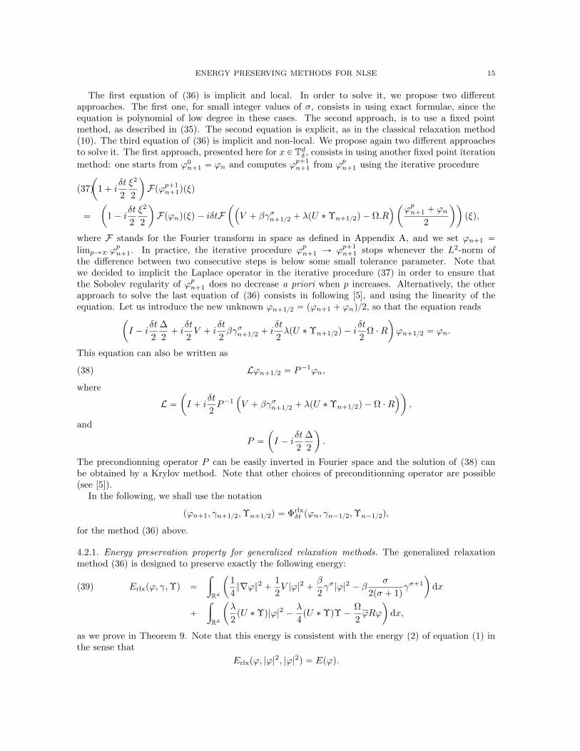
We present on Figure 1 the evolution of EE,δt for various δt when σ “ 2 and σ “ 3 for both classicaland generalized relaxation scheme compared to Crank-Nicolson scheme. The initial datum is chosento be ϕinpxq “ expp´x2q and β “ ´1. The time-space domain is r0, 12s ˆ r´30, 30s. We considerperiodic boundary conditions and the interval r´30, 30s is meshed with 213` 1 nodes. As it is known,the standard relaxation scheme does not preserve the energy when σ “ 2 or σ “ 3 and the error curve


show a second order convergence. On the other hand, both generalized relaxation and Crank-Nicolsonpreserve energy to epsilon machine.

σ “ 2,

10´4 10´3 10´2 10´110´16

10´12

10´8

10´4

δt

E E,δt

Classical relaxationGeneralized relaxationCrank NicolsonSlope 2

σ “ 3,

10´4 10´3 10´2 10´110´16

10´12

10´8

10´4

δt

E E,δt

Figure 1. EE,δt for relaxation schemes and Crank-Nicolson scheme when σ “2 and σ “ 3

5.2. A nonlocal Schrodinger equation with cubic-quintic nonlinearities. In [13], Chen et al.investigate the interactions of dark solitons under competing nonlocal cubic and local quintic nonlin-earities. They consider a 1D optical beam with an amplitude ϕpt, xq with competing nonlocal cubicand local quintic nonlinearities. Their model is given by the following nonlocal nonlinear Schrodingerequation

(50) Btϕpt, xq “ i

ˆ

1

2B2x ` α1U ˚ |ϕpt, xq|

2 ` α2|ϕpt, xq|4

˙

ϕpt, xq, ϕp0, xq “ ϕin,

where Upxq is the nonlocal kernel and α1 and α2 are real parameters. When αj ą 0, j “ 1, 2, weare considering focusing nonlinearities, whereas when αj ă 0, the nonlinearities are defocusing. Thismodel is generalized in two dimensions in [25] for the study of vortex solitons where B2x is replaced bythe two-dimensional Laplace operator. Typically, the kernel is regular and is given by

(51) U1pxq “1t|x|ďµu

p2µqd, x P Rd,

or

(52) U2pxq “1

pµ?πqd

exp`

´|x|2µ2˘

, x P Rd,


the parameter µ allowing to control the width of the kernel, or in other words, the nonlocality strength.At the limit µÑ 0, the kernel Uj , j “ 1, 2, tends to a Dirac distribution and we recover a local nonlinearmodel. The equation (50) is associated to the energy

(53) Epϕqptq “1

2

ż

R

ˆ

1

2∇ϕ2 ´ α1

2pU ˚ |ϕ|2q|ϕ|2 ´

α2

3|ϕ|6

˙

dx.

We reproduce the numerical experiments presented in [13, 25] and show the ability of the generalizedrelaxation method to preserve the energy (39) in the form (56) below. The generalized relaxationmethod for (50) consists in approximating the system of equations

(54)

$

’

’

’

’

&

’

’

’

’

%

Υ “ |ϕ|2,

γ2 “ |u|4,

iBtϕ “

ˆ

´1

2∆´ α1U ˚Υ´ α2γ

2

˙

ϕ,

and the numerical scheme reads

(55)

$

’

’

’

’

&

’

’

’

’

%

Υn`12 “ 2|ϕn|2 ´Υn´12,

γ2n`12 “

ˆ

3

2|ϕn|

2 ´ γn´12

˙

pγn´12 ` γn`12q,

iϕn`1 ´ ϕn

δt“ ´

1

2∆ϕn`1 ´ ϕn

2´

´

α1U ˚Υn`12 ` α2γ2n`12

¯ ϕn`1 ` ϕn2

,

with ϕ0pxq “ ϕinpxqq and Υ´12pxq “ γ´12pxq is some second order approximation of ϕp´δt2, xq.In our numerical experiments, this approximation is obtained by applying the Crank-Nicolson schemestarting from ϕ0 on reverse time step ´δt2. The energy associated to (54) is

(56) Erlxpϕ, γ,Υq “1

2

ż

R

ˆ

1

2∇ϕ2 ´ α1U ˚Υp|ϕ|2 ´

Υ

2q ´ α2γ

2p|ϕ|2 ´2

3ϕq

˙

dx

and we have the conservation property (40).We are first interested in the one-dimensional case with kernel U1 and we choose a defocusing

nonlocal nonlinearity by considering α1 “ ´1. Like in the previous subsection, the space variable isdiscretized using Fourier spectral approximation and we consider periodic boundary conditions. Inorder to avoid any interaction between the nonlocal kernel and the boundaries, we take a very largedomain, typically x P r´256π, 256πs discretized with J “ 214` 1 nodes. The time step is δt “ 5 ¨ 10´3

and the final time is T “ 30. The initial datum is made of two solitons at a relative distance of 2x0,where x0 “ 1. Following [13], we choose

ϕinpxq “ tanhpDpx´ x0qqtanhpDpx` x0qq,

where D is the positive root of the equation

cothpDµq

Dµ

„

1

D2´ µ2csch2

pDµq

´11

15

2α2

3D2“

1

3.

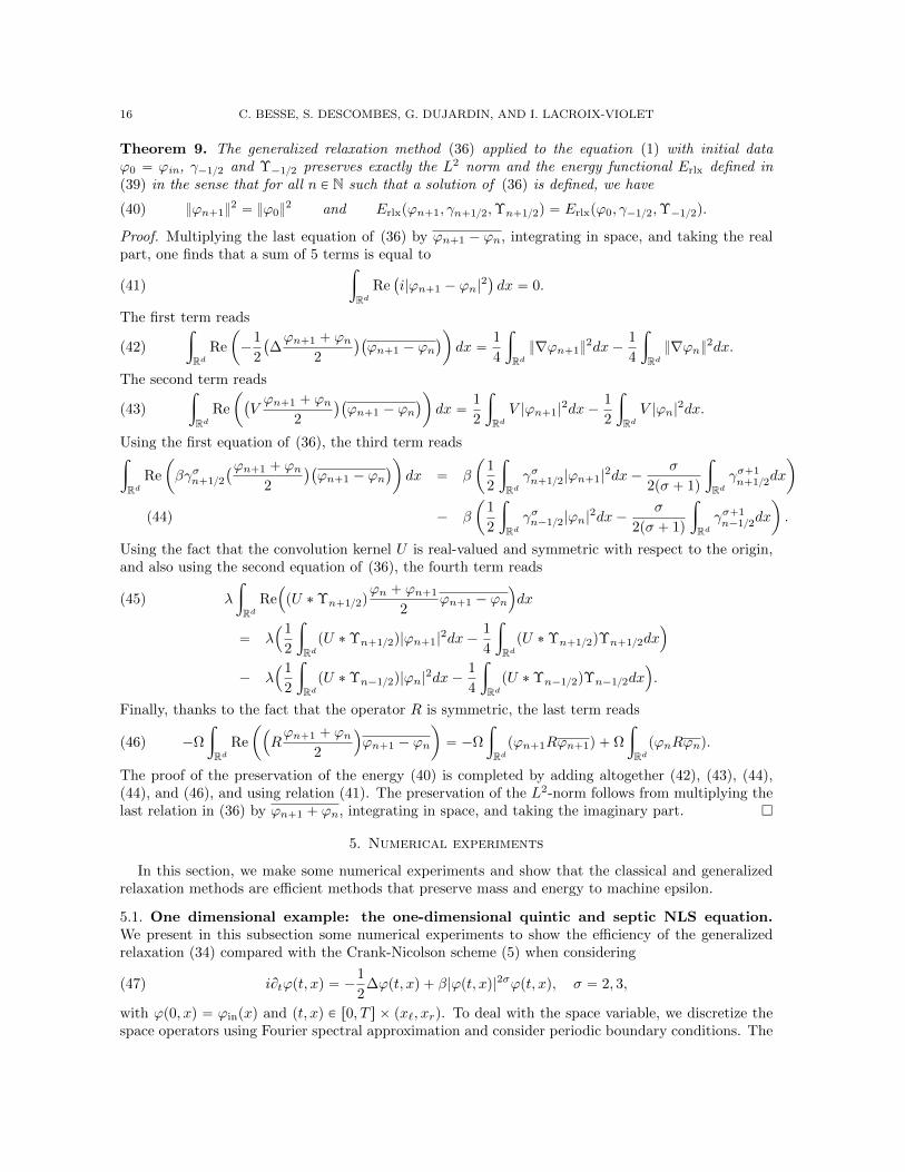
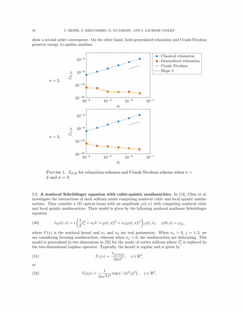
We present results in Figure 2 and 3 for a defocusing cubic nonlinearity α2 “ ´0.5 and a focusing onewhere α2 “ 0.1. Two values for µ are proposed µ “ 0.5 and µ “ 2.5. The behavior of the defocusing-defocusing case is surprising for “strong” nonlocality µ “ 2.5 since eventually the two solitons breathe.

The evolution of the relative energy error

(57)

ˇ

ˇErlxpϕn, γn´12,Υn´12q ´ Erlxpϕ0, γ´12,Υ´12qˇ

ˇ

Erlxpϕ0, γ´12,Υ´12q

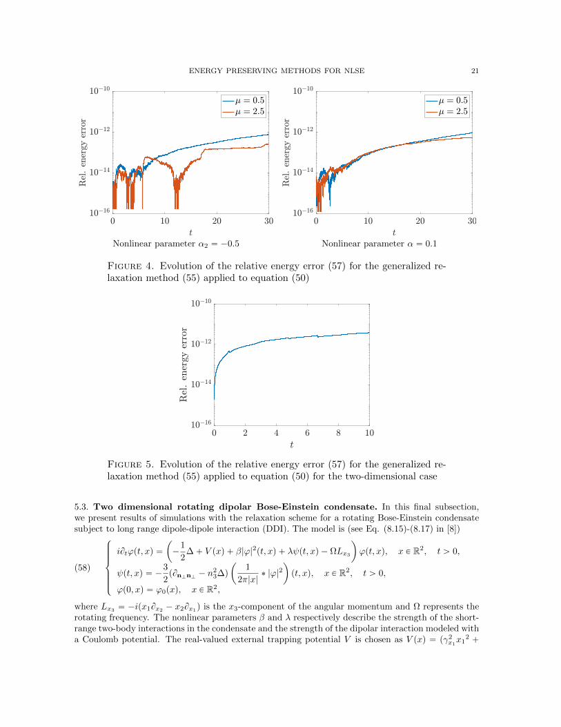
is presented on Figure 4. The energy is clearly very well preserved.


µ “ 0.5 µ “ 2.5

Figure 2. Solutions |ϕn|2 of the generalized relaxation method (55) applied

to equation (50) at time T “ 30 for α2 “ ´0.5, µ “ 0.5 and µ “ 2.5.

µ “ 0.5 µ “ 2.5

Figure 3. Solutions |ϕn|2 of the generalized relaxation method (55) applied

to equation (50) at time T “ 30 for α2 “ 0.1, µ “ 0.5 and µ “ 2.5.

Concerning the two dimensionsal case, we consider the kernel U2, α1 “ 1 and α2 “ ´0.02. Theinitial datum is chosen as a vortex beam with angular momentum

ϕinpx1, x2q “ Arme´r22eimφ,

where r “a

x21 ` x22, m “ 1 is the topological charge, φ is such that x1` ix2 “ r exppiφq and A “ 5.8

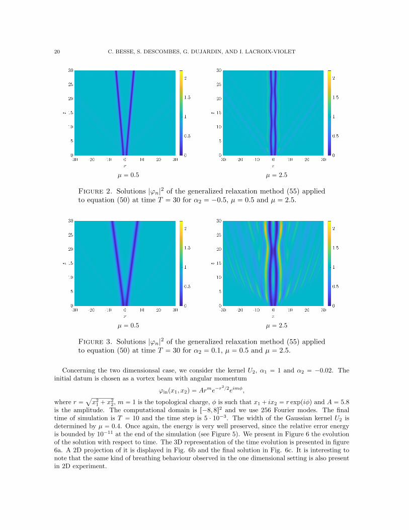
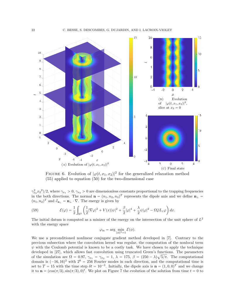
is the amplitude. The computational domain is r´8, 8s2 and we use 256 Fourier modes. The finaltime of simulation is T “ 10 and the time step is 5 ¨ 10´3. The width of the Gaussian kernel U2 isdetermined by µ “ 0.4. Once again, the energy is very well preserved, since the relative error energyis bounded by 10´11 at the end of the simulation (see Figure 5). We present in Figure 6 the evolutionof the solution with respect to time. The 3D representation of the time evolution is presented in figure6a. A 2D projection of it is displayed in Fig. 6b and the final solution in Fig. 6c. It is interesting tonote that the same kind of breathing behaviour observed in the one dimensional setting is also presentin 2D experiment.


Nonlinear parameter α2 “ ´0.5 Nonlinear parameter α “ 0.1

Figure 4. Evolution of the relative energy error (57) for the generalized re-laxation method (55) applied to equation (50)

Figure 5. Evolution of the relative energy error (57) for the generalized re-laxation method (55) applied to equation (50) for the two-dimensional case

5.3. Two dimensional rotating dipolar Bose-Einstein condensate. In this final subsection,we present results of simulations with the relaxation scheme for a rotating Bose-Einstein condensatesubject to long range dipole-dipole interaction (DDI). The model is (see Eq. (8.15)-(8.17) in [8])

(58)

$

’

’

’

’

&

’

’

’

’

%

iBtϕpt, xq “

ˆ

´1

2∆` V pxq ` β|ϕ|2pt, xq ` λψpt, xq ´ ΩLx3

˙

ϕpt, xq, x P R2, t ą 0,

ψpt, xq “ ´3

2pBnKnK ´ n

23∆q

ˆ

1

2π|x|˚ |ϕ|2

˙

pt, xq, x P R2, t ą 0,

ϕp0, xq “ ϕ0pxq, x P R2,

where Lx3 “ ípx1Bx2 ´ x2Bx1q is the x3-component of the angular momentum and Ω represents therotating frequency. The nonlinear parameters β and λ respectively describe the strength of the short-range two-body interactions in the condensate and the strength of the dipolar interaction modeled witha Coulomb potential. The real-valued external trapping potential V is chosen as V pxq “ pγ2x1

x12 `


(a) Evolution of |ϕpt, x1, x2q|2

(b) Evolutionof |ϕpt, x1, x2q|

2,slice at x2 “ 0

(c) Final state

Figure 6. Evolution of |ϕpt, x1, x2q|2 for the generalized relaxation method

(55) applied to equation (50) for the two-dimensional case

γ2x2x2

2q2, where γx1ą 0, γx2

ą 0 are dimensionless constants proportional to the trapping frequencies

in the both directions. The normal n “ pn1, n2, n3qT represents the dipole axis and we define nK “

pn1, n2qT and BnK “ nK ¨∇. The energy is given by

(59) Epϕq “ 1

2

ż

R2

ˆ

1

2|∇ϕ|2 ` V pxq|ψ|2 ` β

2|ϕ|4 `

λ

2ψ|ϕ|2 ´ ΩϕLzϕ

˙

dx.

The initial datum is computed as a minizer of the energy on the intersection of the unit sphere of L2

with the energy space

ϕin “ arg minφ2“1

Epφq.

We use a preconditioned nonlinear conjugate gradient method developed in [7]. Contrary to theprevious subsection where the convolution kernel was regular, the computation of the nonlocal termψ with the Coulomb potential is known to be a costly task. We have chosen to apply the techniquedeveloped in [27], which allows fast convolution using truncated Green’s functions. The parameters

of the simulation are Ω “ 0.97, γx1“ γx2

“ 1, λ “ 175, β “ p250 ´ λqa

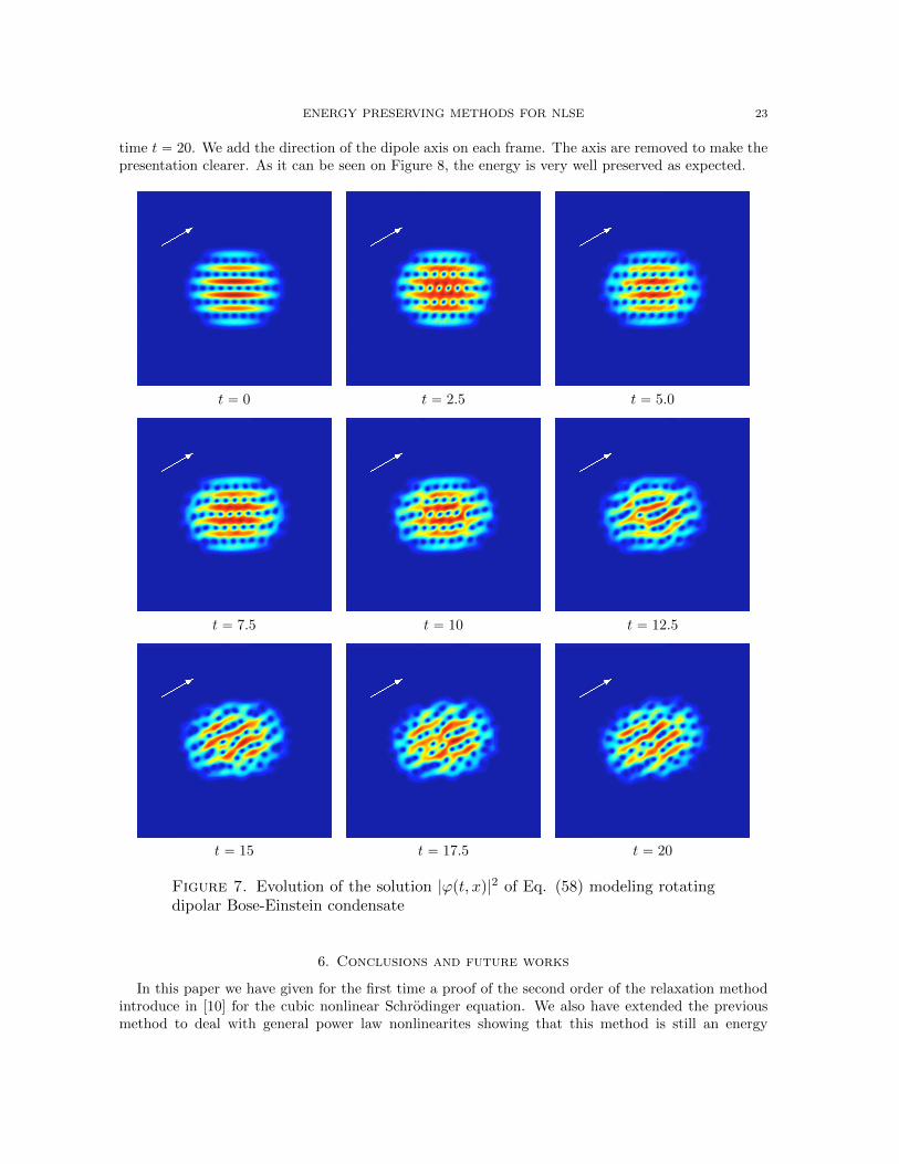
5π. The computationaldomain is p´16, 16q2 with 28 “ 256 Fourier modes in each direction, and the computational time isset to T “ 15 with the time step δt “ 10´3. Initially, the dipole axis is n “ p1, 0, 0qT and we changeit to n “ pcospπ3q, sinpπ3q, 0qt. We plot on Figure 7 the evolution of the solution from time t “ 0 to


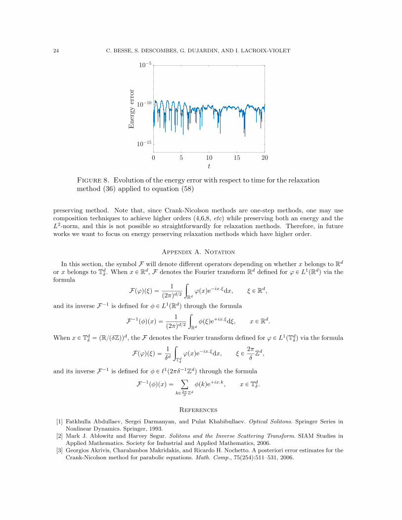
time t “ 20. We add the direction of the dipole axis on each frame. The axis are removed to make thepresentation clearer. As it can be seen on Figure 8, the energy is very well preserved as expected.

t “ 0 t “ 2.5 t “ 5.0

t “ 7.5 t “ 10 t “ 12.5

t “ 15 t “ 17.5 t “ 20

Figure 7. Evolution of the solution |ϕpt, xq|2 of Eq. (58) modeling rotatingdipolar Bose-Einstein condensate

6. Conclusions and future works

In this paper we have given for the first time a proof of the second order of the relaxation methodintroduce in [10] for the cubic nonlinear Schrodinger equation. We also have extended the previousmethod to deal with general power law nonlinearites showing that this method is still an energy


Figure 8. Evolution of the energy error with respect to time for the relaxationmethod (36) applied to equation (58)

preserving method. Note that, since Crank-Nicolson methods are one-step methods, one may usecomposition techniques to achieve higher orders (4,6,8, etc) while preserving both an energy and theL2-norm, and this is not possible so straightforwardly for relaxation methods. Therefore, in futureworks we want to focus on energy preserving relaxation methods which have higher order.

Appendix A. Notation

In this section, the symbol F will denote different operators depending on whether x belongs to Rdor x belongs to Tdδ . When x P Rd, F denotes the Fourier transform Rd defined for ϕ P L1pRdq via theformula

Fpϕqpξq “ 1

p2πqd2

ż

Rdϕpxqeíx.ξdx, ξ P Rd,

and its inverse F´1 is defined for φ P L1pRdq through the formula

F´1pφqpxq “1

p2πqd2

ż

Rdφpξqeìx.ξdξ, x P Rd.

When x P Tdδ “ pRpδZqqd, the F denotes the Fourier transform defined for ϕ P L1pTdδq via the formula

Fpϕqpξq “ 1

δd

ż

Tdδϕpxqeíx.ξdx, ξ P

2π

δZd,

and its inverse F´1 is defined for φ P `1p2πδ´1Zdq through the formula

F´1pφqpxq “ÿ

kP 2πd Zd

φpkqeìx.k, x P Tdδ .

References

[1] Fatkhulla Abdullaev, Sergei Darmanyan, and Pulat Khabibullaev. Optical Solitons. Springer Series inNonlinear Dynamics. Springer, 1993.

[2] Mark J. Ablowitz and Harvey Segur. Solitons and the Inverse Scattering Transform. SIAM Studies inApplied Mathematics. Society for Industrial and Applied Mathematics, 2006.

[3] Georgios Akrivis, Charalambos Makridakis, and Ricardo H. Nochetto. A posteriori error estimates for theCrank-Nicolson method for parabolic equations. Math. Comp., 75(254):511–531, 2006.


[4] Xavier Antoine, Christophe Besse, and Pauline Klein. Numerical solution of time-dependent nonlinearschrdinger equations using domain truncation techniques coupled with relaxation scheme. Laser Physics,21(8):1–12, 2011.

[5] Xavier Antoine and Romain Duboscq. Robust and efficient preconditioned Krylov spectral solvers for com-puting the ground states of fast rotating and strongly interacting Bose-Einstein condensates. J. Comput.Phys., 258:509–523, 2014.

[6] Xavier Antoine and Romain Duboscq. Modeling and computation of Bose-Einstein condensates: stationarystates, nucleation, dynamics, stochasticity. In Nonlinear optical and atomic systems, volume 2146 ofLecture Notes in Math., pages 49–145. Springer, Cham, 2015.

[7] Xavier Antoine, Antoine Levitt, and Qinglin Tang. Efficient spectral computation of the stationary statesof rotating Bose-Einstein condensates by preconditioned nonlinear conjugate gradient methods. J. Comput.Phys., 343:92–109, 2017.

[8] Weizhu Bao and Yongyong Cai. Mathematical theory and numerical methods for Bose-Einstein conden-sation. Kinet. Relat. Models, 6(1):1–135, 2013.

[9] Weizhu Bao, Daniel Marahrens, Qinglin Tang, and Yanzhi Zhang. A simple and efficient numerical methodfor computing the dynamics of rotating Bose-Einstein condensates via rotating Lagrangian coordinates.SIAM J. Sci. Comput., 35(6):A2671–A2695, 2013.

[10] Christophe Besse. Analyse numerique des systemes de Davey-Stewartson. PhD thesis, Universite Bordeaux1, 1998.

[11] Christophe Besse. A relaxation scheme for the nonlinear Schrodinger equation. SIAM J. Numer. Anal.,42(3):934–952 (electronic), 2004.

[12] Sulem Catherine and Sulem Pierre-Louis. The Nonlinear Schrodinger Equation: Self-Focusing and WaveCollapse, volume 139. Springer Science and Business Media, 2007.

[13] Wei Chen, Ming Shen, Qian Kong, Jielong Shi, Qi Wang, and Wieslaw Krolikowski. Interactions ofnonlocal dark solitons under competing cubic-quintic nonlinearities. Optics Letters, 39(1):1764–1767, 1014.

[14] J. Crank and P. Nicolson. A practical method for numerical evaluation of solutions of partial differentialequations of the heat-conduction type. Proc. Cambridge Philos. Soc., 43:50–67, 1947.

[15] Morten Dahlby and Brynjulf Owren. Plane wave stability of some conservative schemes for the cubicSchrodinger equation. M2AN Math. Model. Numer. Anal., 43(4):677–687, 2009.

[16] Thierry Dauxois and Michel Peyrard. Physics of Solitons. Cambridge University Press, 2006.[17] M. Delfour, M. Fortin, and G. Payre. Finite-difference solutions of a nonlinear Schrodinger equation. J.

Comput. Phys., 44(2):277–288, 1981.[18] Maxime Gazeau. Probability and pathwise order of convergence of a semidiscrete scheme for the stochastic

Manakov equation. SIAM J. Numer. Anal., 52(1):533–553, 2014.[19] Jean Ginibre and Giorgio Velo. On a class of nonlinear schrodinger equations part i, ii. J. Funct. Anal.,

32:1–32, 33–71, 1979.[20] Patrick Henning and Johan Warnegard. Numerical comparison of mass-conservative schemes for the gross-

pitaevskii equation, 2018.[21] John Holte. Discrete Gronwall lemma. In MAA-NCS meeting at the University of North Dakota, 2009.[22] Dietmar Oelz and Saber Trabelsi. Analysis of a relaxation scheme for a nonlinear Schrodinger equation

occurring in plasma physics. Math. Model. Anal., 19(2):257–274, 2014.[23] Lev Pıtajevskıj and Sandro Stringari. Bose-Einstein Condensation. Clarendon Press, Oxford, 2003.[24] J. M. Sanz-Serna. Methods for the numerical solution of the nonlinear Schroedinger equation. Math.

Comp., 43(167):21–27, 1984.[25] Ming Shen, Di Wu, Hongwei Zhao, , and Bailing Li. Vortex solitons under competing nonlocal cubic and

local quintic nonlinearities. Journal of Physics B: Atomic, Molecular and Optical Physics, 47, 2014.[26] Walter Strauss and Luis Vazquez. Numerical solution of a nonlinear Klein-Gordon equation. J. Comput.

Phys., 28(2):271–278, 1978.[27] Felipe Vico, Leslie Greengard, and Miguel Ferrando. Fast convolution with free-space Green’s functions.

J. Comput. Phys., 323:191–203, 2016.[28] Dongling Wang, Aiguo Xiao, and Wei Yang. Crank-Nicolson difference scheme for the coupled nonlinear

Schrodinger equations with the Riesz space fractional derivative. J. Comput. Phys., 242:670–681, 2013.


(C. Besse) Institut de Mathematiques de Toulouse, UMR5219, Universite de Toulouse, CNRSUPS IMT, F-31062 Toulouse Cedex 9, France

E-mail address: [email protected]

(S. Descombes) Universite Cote d’Azur, CNRS, INRIA, LJAD, FranceE-mail address: [email protected]

(G. Dujardin) Inria, Univ. Lille, CNRS, UMR 8524, Laboratoire Paul Painleve, F-59000 Lille,France


(I. Lacroix-Violet) Laboratoire Paul Painleve, CNRS UMR 8524, INRIA RAPSODI Team, Uni-versite de Lille 1, Cite Scientifique, 59655 Villeneuve d’Ascq Cedex, France


Documents

Energy preserving methods for nonlinear Schrödinger equations