Energy management - Basic knowledge Technical Information

Energy management - Basic knowledge Technical InformationLet’s connect.

Measuring and monitoring systems

Contents

Energy management - Basic knowledge Contents

2 Harmonics

5 Current / voltage unbalance

6 Transients

7 Voltage dips and interruptions

9 Phase shifting and reactive power

10 Power factor correction

• Basics for power factor correction• Calculation formula for the capacitor

15 RCM – Residual Current Monitoring

17 Collection of formulas

24 Current transformer

• General information on current transformers• Selecting current transformers• Current transformer construction types• Installation of current transformers• Operation of current transformers

34 Communication via the RS485 interface

42 Ports, protocols and connections

44 Overvoltage categories

46 Valid standards

1

Harmonics

The constantly rising number of non-linear loads in our power networks is causing increasing "noise on the grid". One also speaks of grid distortion effects, similar to those that arise in the environment due to water and air pollution. Generators ideally produce purely sinusoidal form current at the output terminals. This sinusoidal current form is considered the ideal alternating current form and any deviation from this is designated mains interference.

An increasing number of loads are extracting non-sinusoidal current from the grid. The FFT-Fast-Fourier-Transformation of this "noisy" current form results in a broad spectrum of harmonic frequencies - often also referred to as harmonics.

Harmonics are damaging to electrical networks, sometimes even dangerous, and connected loads are harmed by these; in a similar way to the unhealthy effect that polluted water has on the human body. This results in overloads, reduced service lives and in some cases even the early failure of electrical and electronic loads.

Harmonic loads are the main cause of invisible power quality problems and result in massive maintenance and investment costs for the replacement of defective devices. Grid distortion effects of an impermissible high level and the resultant poor power quality can therefore lead to problems in production processes and even to production downtimes.

Harmonics are currents or voltages whose frequency lies above the 50/60-Hz mains frequency, and which are many times this mains frequency. Current harmonics have no portion of the effective power, they only cause a thermal load on the network. Because harmonic currents flow in addition to "active" sinusoidal oscillations, they cause electrical losses within the electrical installation. This can lead to thermal overloads. Additionally, losses in the load lead to heating up or overheating, and therefore to a reduction in the service life.

Fig.: Grid distortion effects through frequency converters

Fig.: Harmonics analysis (FFT)

Threshold values of individual harmonic voltages at the transition point up to the 25th order as a percentage of the fundamental oscillation U1Odd harmonics Even harmonics

No multiple of 3 Multiple of 3Order h

Relative voltage amplitudeUh

Order h


Order h


5 6.0 % 3 5.0 % 2 2.0 %7 5.0 % 9 1.5 % 4 1.0 %11 3.5 % 15 0.5 % 6 bis 24 0.5 %13 3.0 % 21 0.5 %17 2.0 %19 1.5 %23 1.5 %25 1.5 %

1

2

Spannungsverlauf (V)

Stromverlauf (A)

Voltage progression

Current progression

Harmonics

2

The assessment of harmonic loads usually takes place at the connection or transition point to the public mains supply network of the respective energy supplier. One speaks in this case of a Point of Common Coupling (PCC). Under certain circumstances it may also be important to determine and analyse the harmonic load through individual operating equipment or equipment groups, in order to indicate internal power quality problems and possibly determine their causes.

The following parameters are used to assess harmonic loads:

Total Harmonic Distortion (THD)

Total Harmonic Distortion (THD) is a means of quantifying the proportion of distortion arising due to the non-linear distortion of an electrical signal. It therefore gives the ratio of the effective value of all harmonics to the effective value of the mains frequency. The THD value is used in low, medium and high voltage systems. Conventionally, THDi is used for the distortion of current, and THDu for the distortion of voltage.

THD for voltage

• M = Ordinal number of harmonics• M = 40 (Energy Meter D650, Energy Analyser D550, Energy Meter 750)• M = 63 (Energy Analyser D550)• Mains frequency fund equals n = 1

THD for current

• M = Ordinal number of harmonics• M = 40 (Energy Meter D650, Energy Analyser D550, Energy Meter 750)• M = 63 (Energy Analyser 550)• Mains frequency fund equals n = 1

Abb.: Zerstörte Kondensatoren durch Oberschwingungen

THDU = 1⎥Ufund⎥

M∑n=2

⎥Un.Harm⎥2

THDI = 1⎥Ifund⎥

M∑n=2

⎥In.Harm⎥2

Harmonics

3

Total Demand Distortion (TDD)

In North America in particular, the expression TDD is commonly used in conjunction with the issue of harmonics. It is a figure that refers to THDi, although in this case the total harmonic distortion is related to the fundamental oscillation portion of the nominal current value. The TDD therefore gives the relationship between the current harmonics (analogous to the THDi) and the effective current value under full load conditions that arises within a certain interval. Standard intervals are 15 or 30 minutes.

TDD (I)

• TDD gives the relationship between the current harmonics (THDi) and the effective current value with a full load.

• IL = Full load current• M = 40 (Energy Meter D650, Energy Meter 750, Energy Analyser D550)• M = 63 (Energy Analyser 550)

Harmonics

TDD = 1IL

M∑n=2

I2n x 100%

Harmonics

4

One speaks of balance in a three-phase system if the three phase voltages andcurrents are of an equal size and are phase-shifted at 120° to each other..

Unbalance arises if one or both conditions are not fulfilled. In the majorityof cases the cause of unbalance lies in the loads..

In high and medium voltage power grids the loads are usually three-phase andsymmetrical, although large one- or two-phase loads may also be present here(e.g. mains frequency induction furnaces, resistance furnaces, etc.). In the lowvoltage network electrical loads are frequently also single-phase (e.g. PCs,consumer electronics, lighting systems, etc.), and the associated load currentcircuits should be distributed as evenly as possible within the electrical wiringon the three phase conductors. Depending on the symmetry of the singlephaseloads, the network is operated on a more balanced or unbalanced basis.

The compatibility level for the degree of unbalance of the voltage in stationaryoperation caused by all mains loads is defined as ≤ 2 %. Related to individualload systems the resultant degree of unbalance is limited to = 0.7 %, wherebyan average over 10 minutes must be obtained.

The following effects arise due to unbalance in the voltage:

• Increased current loading and losses in the network.• With equal load power the phase currents can attain 2 to 3 times the value,

the losses 2 to 6 times the value. It is then only possible to load lines and transformers with half or one third of their rated power.

• Increased losses and vibration moments in electrical machinery.• The field built up by the negative sequence component of the currents runs

against the phase sequence of the rotor and therefore induces currents in it, which lead to increased thermal loading.

• Rectifiers and inverters react to unbalance in the power supply with uncharacteristic harmonic currents.

• In three-phase systems with star connection, current flows through the neutral conductor.

You can find the related detailed formulas in the collection of formulas.

Current / voltage unbalance

Fig.: Balance

Fig.: Unbalance

Fig.: Illustration of unbalance in the Vector diagram

U1

U3U2

120°120°

120°Ia

Ic

Ib

Ia

Ic

Ib

1

-1

-0.5

0.5

0

Time

1

1.5

-1

-1.5

-0.5

0.5

0

Time

120°120°

120°Ia

Ic

Ib

Ia

Ic

Ib

1

-1

-0.5

0.5

0

Time

1

1.5

-1

-1.5

-0.5

0.5

0

Time

Current / voltage unbalance

5

Transient

t

U

Fig.: Transients

Fig.: With the Energy Analyser 550 it is possible to display the transients directly on the measuring device.

Transients are pulsed electrical phenomena, which exist for just a short period of time. These are usually high frequency, steep signals in the form of transient oscillations.

The reliable detection of transient processes in the electrical supply network is very important in order to avoid damages. Through constant changes in the electrical supply network due to switching operations and faults, new network states arise constantly, which the entire system is required to tune itself to. In normal cases transient compensation currents and compensation voltages arise here. In order to assess whether the transient processes result from a desired or undesired change in the network, and whether these still lie in the tolerance range, one requires reliable decision criteria.

High transient overvoltage, and high dV/dt-ratios, can lead to insulation damage and the destruction of systems and machines, also depending on the energy input (e.g. lightening strike).

In order to detect and record transients it is necessary to use high quality, digital power quality analysers with a high sampling rate.

Practical example:

High transient currents often arise due to the switching – in of capacitors (without reactors or damping facility) – also with problem-free network configurations. Choking has a strongly damping effect and therefore protects against avoidable problems that are difficult to foresee. Alternatively, special capacitor contactors or switching devices should be used, e.g. with pre-charging resistors at LV side.

Transients

Transients

6

Voltage drops can lead to huge complications – for example the failureof production processes – and to quality problems. Such voltage drops arisemuch more frequently than interruptions. The commercial effects of voltagedrops are seriously underestimated time and again..

What is a voltage drop?

According to the European standard EN 50160 a voltage drop is a suddenlowering of the effective voltage value to a value of between 90% and 1%of the stipulated nominal value, followed by the immediate reinstatement ofthis voltage. The duration of a voltage drop lies between a half period (10 ms)and one minute.

If the effective value of the voltage does not drop below 90% of the stipulatedvalue then this is considered to be normal operating conditions. If the voltagedrops below 1% of the stipulated value then this is considered an interruption.

A voltage drop should therefore not be confused with an interruption.An interruption arises, for example, after a circuit breaker has tripped(typ. 300 ms). The mains power failure is propagated throughout the remainingdistribution network as a voltage drop.

The diagram clarifies the difference between a drop, a short interruption and anundervoltage situation.

Voltage dips and interruptions

Overvoltage

Undervoltage

Long interruptionShort interruption

Voltagedips

Normal operating voltage

Ueff

(%)

90

1

10 ms 1 min 3 mint

100

110


7

Voltage variations are caused by:

• Short circuits• Switch-on and switch-off processes with large loads• Starting drives (larger load)• Load changes with drives• Pulsed power (oscillation package controls, thermostatic controls)• Arc furnaces• Welding machines• Switching on capacitors

Voltage drops can lead to the failure of computer systems, PLC systems, relays and frequency converters. With critical processes just a single voltage drop can result in high costs, continuous processes are particularly impacted by this. Examples of this are injection moulding processes, extrusion processes, printing processes or the processing of foodstuffs such as milk, beer or beverages.

The costs of a voltage drop are comprised of:

• Loss of profits due to production stoppage• Costs for catching up with lost production• Costs for delayed delivery of products• Costs for raw materials wastage• Costs for damage to machinery, equipment and moulds• Maintenance and personnel costs

Sometimes processes run in unmanned areas in which voltage drops are not immediately noticed. In this case an injection moulding machine, for example, could come to a complete standstill unnoticed. If this is discovered later there will already be a large amount of damage. The customer receives the products too late and the plastic in the machine has hardened off.

Dip zone 1

Dip zone 2Output field impedance Z1

Supply field impedance Z

Mains transformer

Z2I > In

10 kV

400 V

Z3

Low voltage main distribution

Fig.: Motor start-up currents can lead to a voltage dip

Fig.: Critical voltage dip with production standstill



8

Reactive power is required in order to generate electromagnetic fields in machines such as three phase motors, transformers, welding systems, etc. Because these fields build up and break down continuously, the reactive power swings between generator and load. In contrast to the effective power it cannot be used, i.e. converted into another form of energy, and burdens the supply network and the generator systems (generators and transformers). Furthermore, all energy distribution systems for the provision of the reactive current must exhibit larger dimensions.

It is therefore expedient to reduce the inductive reactive power arising close to the load through a counteractive capacitive reactive power, of the same size where possible. This process is referred to as power factor correction. With power factor correction, the proportion of inductive reactive power in the network reduces by the reactive power of the power capacitor of the power factor correction system (PFC). The generator systems and energy distribution equipment are thereby relieved of the reactive current. The phase shifting between current and voltage is reduced or, in an ideal situation with a power factor of 1, entirely eliminated.

The power factor is a parameter that can be influenced by mains interference such as distortion or unbalance. It deteriorates with progressive phase shifting between current and voltage and with increasing distortion of the current curve. It is defined as a quotient of the sum of the effective power and apparent power, and is therefore a measure of the efficiency with which a load utilises the electrical energy. A higher power factor therefore constitutes better use of the electrical energy and ultimately also a higher degree of efficiency.

Power Factor (arithmetic)

• The power factor is unsigned

cos phi – Fundamental Power Factor

• Only the fundamental oscillation is used in order to calculate the cos phi

• cos phi sign (φ): – = for delivery of effective power + = for consumption of active power

Because no uniform phase shifting angle can be cited with harmonic loading, the power factor λ and the frequently used effective factor cos (φ1) must not be equated with each other. Starting with the formula with I1 = fundamental oscillation effective value of the current, I = total effective value of the current, g1 = fundamental oscillation content of the current and cos (φ1) = shifting factor, one sees that only with sinusoidal form voltage and current (g = 1) is the power factor λ the same as the shifting factor cos(φ1).As such, exclusively with sinusoidal form currents and voltages is the power factor λ the same as the cosine of the phase shifting angle φ and is defined as = effective factor.

Phase shifting and reactive power

Fig.: Phase shifting between current and voltage (∆φ)

Active power meterApparentpower(cos φ = 1)

Reactivepower meter Capacitor for compensation

PGrid S

Fig.: Principle of power factor correction

Fig.: Power Factor (arithmetic)

Fig.: cos phi – Fundamental Power Factor

1 π 2π

ωt

∆φ

U

I

PFA =⎥P⎥SA

PF1 = cos (φ) = P1

S1

Phase shifting and reactive power

9

Active power

If one connects an effective resistor, e.g. a heating device, in an alternating current circuit then the current and voltage are in phase. The momentary power values (P) are determined with alternating current through the multiplication of associated momentary values of current (I) and voltage (U). The course of the active power is always positive with doubled mains frequency.

The AC power has the peak value P = U x I. Through area conversion it can be converted into the equivalent DC power, the so-called active power P. In the event of effective resistance, the active power is half the size of the peak power value.

In order to determine the AC power, one always calculates using the effectivevalues.

Active and reactive power

A purely ohmic load rarely arises in practice. An inductive component usually also arises. This applies to all loads, which require a magnetic field in order to function (e.g. motors, transformers, etc.). The current used, which is required in order to generate and reverse the polarity of the magnetic field, is not dissipated but flows back and forth as reactive current between the generator and the load.

Phase shifting arises, i.e. the zero point transitions for voltage and current are no longer congruent. With an inductive load the current follows the voltage, with a capacitive load the relationship is precisely the opposite. If one now calculates the momentary power values (P = U x I), negative values will always arise if one of the two factors is negative.

Example:Phase shifting φ = 45° (equates to an inductive cos φ = 0.707).The power curve overlaps in the negative range.

Basics for power factor correction

P

Uφ = 0° ωt

P: U: I:

Fig.: AC power with purely ohmic load

P: U: I:

φ = 45

P

U

ωt

Fig.: Voltage, current and power with mixed ohmic, inductive load

Fig.: Active power formula

Fig.: Calculation of the effective power with ohmic and inductive load

P = U • I • cos φ[W] [V] [A]

P = U • I[W] [V] [A]

Power factor correction

10

Reactive power

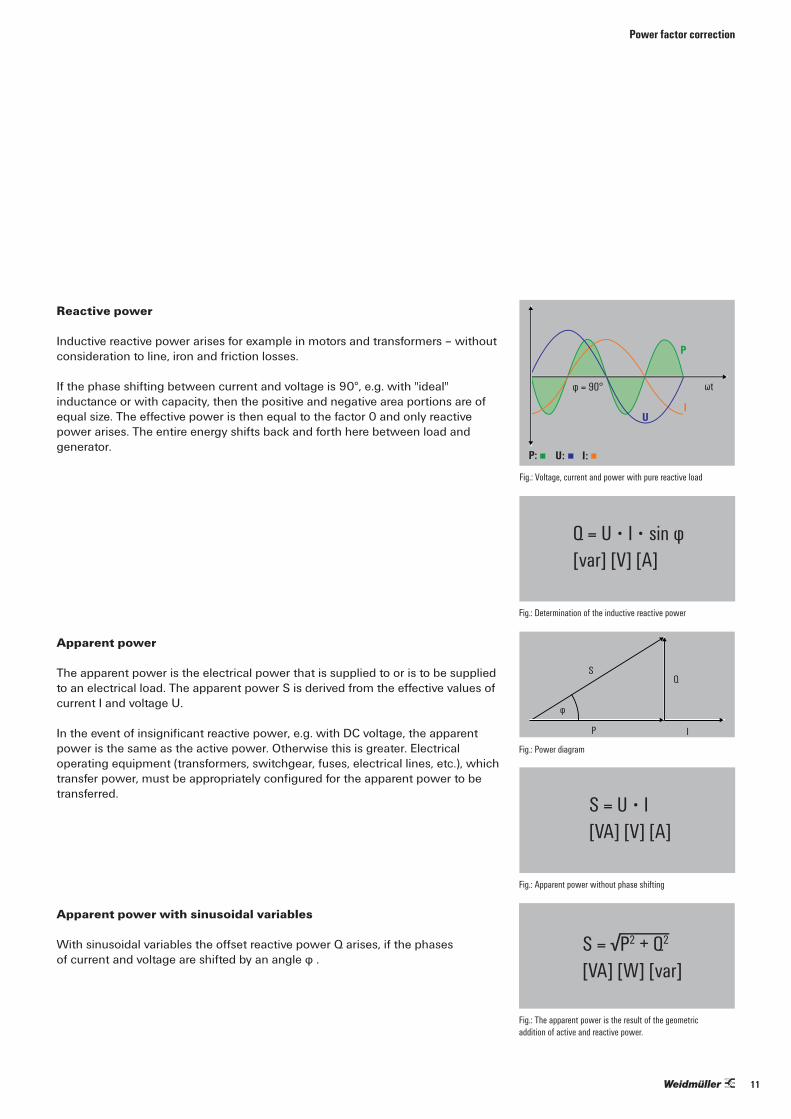
Inductive reactive power arises for example in motors and transformers – without consideration to line, iron and friction losses.

If the phase shifting between current and voltage is 90°, e.g. with "ideal" inductance or with capacity, then the positive and negative area portions are of equal size. The effective power is then equal to the factor 0 and only reactive power arises. The entire energy shifts back and forth here between load and generator.

Apparent power

The apparent power is the electrical power that is supplied to or is to be supplied to an electrical load. The apparent power S is derived from the effective values of current I and voltage U.

In the event of insignificant reactive power, e.g. with DC voltage, the apparent power is the same as the active power. Otherwise this is greater. Electrical operating equipment (transformers, switchgear, fuses, electrical lines, etc.), which transfer power, must be appropriately configured for the apparent power to be transferred.

Apparent power with sinusoidal variables

With sinusoidal variables the offset reactive power Q arises, if the phasesof current and voltage are shifted by an angle φ .

P: U: I:

φ = 90°

P

U

ωt

φ

SQ

P I

Fig.: Voltage, current and power with pure reactive load

Fig.: Power diagram

Fig.: Determination of the inductive reactive power

Fig.: Apparent power without phase shifting

Fig.: The apparent power is the result of the geometricaddition of active and reactive power.

S = P2 + Q2

[VA] [W] [var]

S = U • I[VA] [V] [A]

Q = U • I • sin φ[var] [V] [A]


11

Power factor (cos φ and tan φ)

The relationship of active power P to apparent power S is referred to as the effective power factor or effective factor. The power factor can lie between 0 and 1.

With pure sinusoidal currents, the effective power factor concurs with the cosine (cos φ). It is defined from the relationship P/S. The effective power factor is a measure through which to determine what part of the apparent power is converted into effective power. With a constant effective power and constant voltage the apparent power and current are lower, the greater the active power factor cos φ.

The tangent (tan) of the phase shift angle (φ) facilitates a simple conversion of the reactive and effective unit.

The cosine and tangent exist in the following relationship to each other:

In power supply systems the highest possible power factor is desired, in order to avoid transfer losses. Ideally this is precisely 1, although in practical terms it is around 0.95 (inductive). Energy supply companies frequently stipulate a power factor of at least 0.9 for their customers. If this value is undercut then the reactive energy utilised is billed for separately. However, this is not relevant to private households. In order to increase the power factor, systems are used for power factor correction. If one connects the capacitor loads of a suitable size in parallel then the reactive power swings between the capacitor and the inductive load. The superordinate network is no longer additionally loaded. If, through the use of PFC, a power factor of 1 should be attained, only the effective current is still transferred.

The reactive power Qc, which is absorbed by the capacitor or dimensioned for this capacitor, results from the difference between the inductive reactive power Q1 before correction and Q2 after correction.

The following results: Qc = Q1 – Q2

φ1

SQc

Q2

P I

φ2

Q1

Fig.: Determination of the power factor over effective and apparent power

Fig.: Power diagram with application of power factor correction

Fig.: Calculation of the phase shifting over reactive and effective power

Fig.: Relationship to cos φ and tan φ

Fig.: Calculation of the reactive power for the improvement of the power factor

QC = P • (tan φ1 - tan φ2

[var] [W]

cos φ = 11 + tan φ2

cos φ = PS

[W] / [VA]

tan φ = QP

[var] / [W]


Basics for power factor correction

12

Calculation formula for the capacitor

Capacitor output single-phase

Example: 66.5 μF with 400 V / 50 Hz0.0000665 · 400² · 2 · 3.14 · 50 = 3.340 var = 3.34 kvar

Capacitor output with delta connection

Example: 3 x 57 μF with 480 V / 50 Hz3 · 0.000057 · 480² · 2 · 3.14 · 50 = 12.371 var = 12.37 kvar

Capacitor output with star connection

Example: 3 x 33.2 μF with 400 V / 50 Hz3 · 0.0000332 · (400 / 1.73)² · 2 · 3.14 · 50 = 1670 var = 1.67 kvar

Capacitor current in the phase conductor

Example: 25 kvar with 400 V25.000 / (400 · 1.73) = 36 A

Series resonant frequency (fr) and de-tuning factor (p)of de-tuned capacitors

Example: p = 0.07 (7 % de-tuning) in the 50-Hz network

fr = 50 •1

0,07 = 189 Hz

QC = C • U² • 2 • π • fn

I = QU • 3

QC = I • U • 3

fr = fn • 1p

p = fn

2

fr

QC = 3 • C • U² • 2 • π • fn

QC = 3 • C • (U / 3)² • 2 • π • fn


13

Required nominal capacitor output three-phase in de-tuned configuration

Example: 3 x 308 μF with 400 V / 50 Hz with p = 7 % de-tuned

0.000308 · 3 · 4002 · 2 · 3.14 · 50 / (1 - 0.07) = 50 kvar

Which capacitor should be used for this?This means, for a 50-kvar stage, a 440-V-56-kvar capacitor is required.

Power factor and cos and tan conversion

Conversion of the capacitor power subject of the mains voltage

Determination of the reactive power Qnew · C is constant here.

Example:

Network: 400 V, 50 Hz, 3-phaseNominal capacitor data: 480 V, 70 kvar, 60 Hz, 3-phase, delta, un-chokedQuestion: Resultant nominal capacitor power?

Qneu =

The resultant correction power of this 480-V capacitor connectedto a 400-V-50-Hz network is just 40.5 kvar.

Definition

QC Nominal capacitor powerP Degree of de-tuningUC Capacitor voltageUN Nominal voltageNC Effective filter outputQneu New reactive powerUneu New voltagefneu New frequencyfR Nominal frequency of the capacitor

QC = C • 3 • U² • 2 • π • fn

1 - p

QC =P1 -

100•

UC2

UN2

• NC

cos φ = PS

cos φ = 11 + tan φ2

Qneu = Uneu2

UC•

fneu

fR

• QC


Calculation formula for the capacitor

14

General information

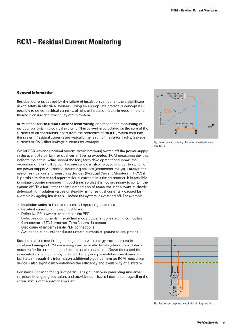
Residual currents caused by the failure of insulation can constitute a significant risk to safety in electrical systems. Using an appropriate protective concept it is possible to detect residual currents, eliminate insulation faults in good time and therefore ensure the availability of the system.

RCM stands for Residual Current Monitoring and means the monitoring of residual currents in electrical systems. This current is calculated as the sum of the currents of all conductors, apart from the protective earth (PE), which feed into the system. Residual currents are typically the result of insulation faults, leakage currents or EMC filter leakage currents for example.

Whilst RCD devices (residual current circuit breakers) switch off the power supply in the event of a certain residual current being exceeded, RCM measuring devices indicate the actual value, record the long-term development and report the exceeding of a critical value. This message can also be used in order to switch off the power supply via external switching devices (contactors, relays). Through the use of residual current measuring devices (Residual Current Monitoring, RCM) it is possible to detect and report residual currents in a timely manner. It is possible to initiate counter measures in good time, so that it is not necessary to switch the system off. This facilitates the implementation of measures in the event of slowly deteriorating insulation values or steadily rising residual currents – caused for example by ageing insulation – before the system is switched off. For example:

• Insulation faults of lines and electrical operating resources• Residual currents from electrical loads• Defective PP power capacitors for the PFC• Defective components in switched mode power supplies, e.g. in computers• Correctness of TNS systems (Terra Neutral Separate)• Disclosure of impermissible PEN connections• Avoidance of neutral conductor reverse currents to grounded equipment

Residual current monitoring in conjunction with energy measurement in combined energy / RCM measuring devices in electrical systems constitutes a measure for fire protection and maintenance prevention. Down times and the associated costs are thereby reduced. Timely and preventative maintenance – facilitated through the information additionally gained from an RCM measuring device – also significantly enhances the efficiency and availability of a system.

Constant RCM monitoring is of particular significance in preventing unwanted surprises in ongoing operation, and provides consistent information regarding the actual status of the electrical system.

Fig.: Report prior to switching off - an aim of residual current monitoring

mA

TimetInformation advantageRe

sidua

l cur

rent

Messagefrom RCM

Switch-offPersonnel protection

System protectionFire protection

RCM – Residual Current Monitoring

L1L2L3

PEN

PE

N

L1 L2 L3 N I1 I2 I3 I4 I5 I6

Energy Meter 750 (RCM)M3~

Differenzstrommessung

Fig.: Fault current to ground through high ohmic ground fault


15

Fundamental measuring process with RCM

The functionality of RCM measuring devices is based on the differential currentprinciple. This requires that all phases be guided through a residual currenttransformer at the measuring point (outlet to be protected), with the exceptionof the protective earth. If there is no failure in the system then the sum of allcurrents will be nil. If, however, residual current is flowing away to ground thenthe difference will result in the current at the residual current transformer beingevaluated by the electronics in the RCM measuring device.

The measurement process is described in IEC/TR 60755. Differentiation is madehere between type A and type B.

DIN EN 62020 / VDE 0663 / IEC 62020 standard:

The standard applies to residual current monitoring devices for domesticinstallations and similar applications with a rated voltage of < 440 V ACand a rated current of < 125 A.

Optimum monitoring through 6 current measurement channels

Modern, highly integrated measuring devices facilitate the combinedmeasurement of• Electrical parameters (V, A, Hz, kW ...)• Power quality parameters (harmonics, THD, SIs ...)• Energy loads (kWh, kvarh ...)• RCM residual current in just one measuring device. The following example

shows a measuring device with 6 current inputs for this purpose:

The Energy Meter 750 can measure residualcurrents in accordance with IEC/TR 60755 (2008-01)

of type A and

type B.

L1 I L2 I L3 I N

Fault current = 0System is OK

Sum > 0Fault in thesystem

L1L2L3

PEN

PE

N

L1 L2 L3 N I1 I2 I3 I4 I5 I6

Energy Meter 750 (RCM)M3~

Residual current monitoring



16

Effective value of the current for phase conductor p

Apparent power for phase conductor p

• The apparent power is unsigned.

Total apparent power (arithmetic)

• The apparent power is unsigned.

Effective voltage L-N

Effective voltage L-L

Neutral voltage (vectorial)

Effective power for phase conductor

Collection of formulas

IP = 1N

•N–1∑k=0

ipk2

Effective value of the neutral conductor current

IN = 1N

•N–1∑k=0

(i1k + i2k + i3k)2

UPN = 1N

•N–1∑k=0

upNk2

Upg = 1N

•N–1∑k=0

(ugNk – upNk)2

UNeutral voltage = U1rms + U2rms + U3rms

Pp = 1N

•

N–1∑k=0

(upNk x ipk)

Sp = UpN • Ip

SA = S1 + S2 + S3


17

THD

• THD (Total Harmonic Distortion) is the distortion factor and gives the relationship of the harmonic portions of oscillation to the fundamental oscillation.

THD for voltage

• M = Ordinal number of harmonics• M = 40 (Energy Meter D650, Energy Meter 750, Energy Analyser D550)• M = 63 (Energy Analyser 550)• Mains frequency fund equals n = 1

Verzerrungsfaktor für den Strom

• M = Ordinal number of harmonics• M = 40 (Energy Meter D650, Energy Meter 750, Energy Analyser D550)• M = 63 (Energy Analyser 550)• Mains frequency fund equals n = 1

ZHD

• ZHD is the THD for interharmonics

Interharmonics

• Sinusoidal form oscillations, whose frequencies are not whole multipliers of the mains frequency (fundamental oscillation)

• Is calculated in the device series UMG 511 and UMG 605• Calculation and measurement processes according to DIN EN 61000-4-30• The ordinal number of an interharmonic equates to the ordinal number of the

next smallest harmonic. For example, the 3rd interharmonic lies between the 3rd and 4th harmonics.

TDD (I)

• TDD (Total Demand Distortion) gives the relationship between the current harmonics (THDi) and the effective current value with full load.

• IL = Full load current• M = 40 (Energy Meter D650, Energy Meter 750, Energy Analyser D550)• M = 63 (Energy Analyser 550)

Ordinal numbers of harmonics


xxx[0] = Fundamental oscillation (50 Hz/60 Hz)xxx[1] = 2nd harmonic (100 Hz/120 Hz)xxx[2] = 3rd harmonic (150 Hz/180 Hz)etc.

THDU = 1⎥Ufund⎥

M∑n=2

⎥Un.Harm⎥2

THDI = 1⎥Ifund⎥

M∑n=2

⎥In.Harm⎥2

TDD = 1IL

M∑n=2

In2 x 100%


18

Ripple control signal U (EN 61000-4-30)

The ripple control signal U (200 ms measured value) is a voltage measured with a carrier frequency specified by the user. Only frequencies below 3 kHz are taken into consideration.

Ripple control signal I

The ripple control signal I (200 ms measured value) is a current measured with a carrier frequency specified by the user. Only frequencies below 3 kHz are taken into consideration.

Positive-negative-zero sequence component

• The proportion of voltage or current unbalance in a three-phase system is labelled with the positive, negative and zero sequence components.

• The symmetry of the three-phase system strived for in normal operation is disturbed by unbalanced loads, faults and operating equipment. - A three-phase system is referred to as exhibiting symmetry if the three phase conductor voltages and currents are of an equal size and are phaseshifted at 120° to each other. If one or both conditions are not fulfilled then the system is deemed unbalanced. Through the calculation of the symmetrical components comprising positive sequence component, negative sequence component and zero sequence component a simplified analysis of an unbalanced fault in a three-phase system is possible.

• Unbalance is a characteristic of the power quality, for which threshold values have been stipulated in international standards (e.g. EN 50160).

Positive sequence component

Negative sequence component

UMit = 13

UL1, fund + UL2, fund • ej 2π3 + UL3, fund • ej 4π

3

UGeg = 13

UL1, fund + UL2, fund • e-j 2π3 + UL3, fund • e-j 4π

3


19

Zero sequence component

A zero sequence component can only arise if a total current is able to flow back via the neutral conductor.

Voltage unbalance

Downward deviation U (EN 61000-4-30)

Downward deviation I

Power Factor (arithmetic)

• The power factor is unsigned.

cos phi – Fundamental Power Factor

• Only the fundamental oscillation is used in order to calculate the cos phi

• cos phi sign: – = for delivery of effective power + = for consumption of effective power

K factor

• The K factor describes the increase in eddy current losses with a harmonics load. In the case of sinusoidal loading of the transformer the K factor = 1. The greater the K factor, the more heavily a transformer can be loaded with harmonics without overheating.


UZero sequence component = 13

UL1, fund + UL2, fund + UL3, fund

Voltage unbalance = UNeg

UPos

Udown =

Udin –

n∑i=1

Urms–down, i2

n [%]Udin

Idown =

I Rated current –

n∑i=1

Irms–down, i2

n [%]IRated current

PFA = ⎥P⎥SA

PF1 = cos (φ) = P1

S1


20

cos phi sum

• cos phi sign: – = for delivery of effective power + = for consumption of effective power

Phase angle Phi

• The phase angle between current and voltage of phase conductor p is calculated and depicted per DIN EN 61557-12.

• The sign of the phase angle corresponds with the sign of the reactive power.

Fundamental oscillation reactive power

The fundamental oscillation reactive power is the reactive power of the fundamental oscillation and is calculated with the Fourier analysis (FFT). The voltage and current do not need to be sinusoidal in form. All reactive power calculations in the device are fundamental oscillation reactive power calculations.

Reactive power sign

• Sign Q = +1 for phi in the range 0 ... 180 ° (inductive)

• Sign Q = -1 for phi in the range 180 ... 360 ° (capacitive)

Reactive power for phase conductor p

• Reactive power of the fundamental oscillation

cos (φ)Sum3 = P1fund + P2fund + P3fund

(P1fund + P2fund + P3fund)2 + (Q1fund + Q2fund + Q3fund)2

cos (φ)Sum4 = P1fund + P2fund + P3fund + P4fund

(P1fund+P2fund+P3fund+P4fund)2 + (Q1fund+Q2fund+Q3fund+Q4fund)2

Sign Q (φp) = +1 if φp ∊ [0°–180°]

Sign Q (φp) = –1 if φp ∊ [180°–360°]

Qfund p = Sign Q (φp) • Sfund p2 – Pfund p

2


21

Total reactive power

• Reactive power of fundamental oscillation

Distortion reactive power

• The distortion reactive power is the reactive power of all harmonics and is calculated with the Fourier analysis (FFT).

• The apparent power S contains the fundamental oscillation and all harmonic portions up to the Mth harmonic.

• The effective power P contains the fundamental oscillation and all harmonic portions up to the Mth harmonic.

• M = 40 (Energy Meter D650, Energy Meter 750, Energy Analyser D550)• M = 63 (Energy Analyser 550)

Reactive energy per phase

Reactive energy per phase, inductive

Reactive energy per phase, capacitive

Reactive energy, sum L1–L3


QV = Q1 + Q2 + Q3

D = S2 – P2 – Q2fund

ErL1 = ∫QL1(t) • t

Er(ind)L1 = ∫QL1(t) • t for QL1(t) > 0

Er(cap)L1 = ∫QL1(t) • t for QL1(t) < 0

ErL1, L2, L3 = ∫(QL1(t) + QL2(t) + QL3(t)) • t


22

Reactive energy, sum L1–L3, inductive

Reactive energy, sum L1–L3, capacitive

Er(ind)L1, L2, L3 = ∫(QL1(t) + QL2(t) + QL3(t)) • t

Er(cap)L1, L2, L3 = ∫(QL1(t) + QL2(t) + QL3(t)) • t

for QL1(t) + QL2(t) + QL3(t) > 0

for QL1(t) + QL2(t) + QL3(t) < 0


23

General information

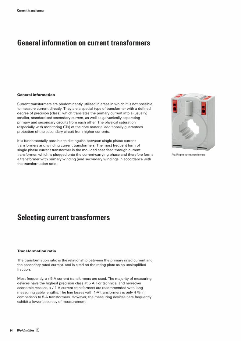
Current transformers are predominantly utilised in areas in which it is not possible to measure current directly. They are a special type of transformer with a defined degree of precision (class), which translates the primary current into a (usually) smaller, standardised secondary current, as well as galvanically separating primary and secondary circuits from each other. The physical saturation (especially with monitoring CTs) of the core material additionally guarantees protection of the secondary circuit from higher currents.

It is fundamentally possible to distinguish between single-phase current transformers and winding current transformers. The most frequent form of single-phase current transformer is the moulded case feed through current transformer, which is plugged onto the current-carrying phase and therefore forms a transformer with primary winding (and secondary windings in accordance with the transformation ratio).

Selecting current transformers

Transformation ratio

The transformation ratio is the relationship between the primary rated current and the secondary rated current, and is cited on the rating plate as an unsimplified fraction.

Most frequently, x / 5 A current transformers are used. The majority of measuring devices have the highest precision class at 5 A. For technical and moreover economic reasons, x / 1 A current transformers are recommended with long measuring cable lengths. The line losses with 1-A transformers is only 4 % in comparison to 5-A transformers. However, the measuring devices here frequently exhibit a lower accuracy of measurement.

General information on current transformers

Fig.: Plug-on current transformers

Current transformer

24

Rated current

Rated or nominal current (earlier designation) is the value of the primary and secondary current cited on the rating plate (primary rated current, secondary rated current), for which the current transformer is dimensioned. Standardised rated currents are (apart from in the classes 0.2 S and 0.5 S) 10 – 12.5 – 15 – 20 – 25 – 30 – 40 – 50 – 60 – 75 A, as well as the decimal multiples and fractions thereof. Standardised secondary currents are 1 and 5 A, preferably 5 A.

Standardised rated currents for the classes 0.2 S and 0.5 S are 25 – 50 – 100 A and their decimal multiples, as well as secondary (only) 5 A.

Correct selection of the primary nominal current is important for the accuracy of measurement. Recommended is a ratio slightly beyond the measured / defined maximum load current (In).

Example: In = 1.154 A; selected transformer ratio = 1.250/5.

The nominal current can also be defined on the basis of the following considerations:

• Dependent on the mains supply transformer nominal current times approx. 1.1 (next transformer size)

• Protection (rated fuse current = CT primary current) of the measured system part (LVDSB, subdistribution boards)

• Actual nominal current times 1.2 (if the actual current lies considerably below the transformer or fuse nominal current then this approach should be selected)

Over-dimensioning the current transformer must be avoided, otherwise the accuracy of measurement significantly decrease especially with small load currents.

Rated power

The rated power of the current transformer is the product of the rated load and the square of the secondary rated current and is quoted in VA. Standardised values are 2.5 – 5 – 10 – 15 – 30 VA. It is also permissible to select values over 30 VA according to the application case. The rated power describes the capacity of a current transformer to "drive" the secondary current within the error limits through a load.

When selecting the appropriate power it is necessary to take into consideration the following parameters: Measuring device power consumption (with connection in series), line length, line cross-section. The longer the line length and the smaller the line cross-section, the higher the losses through the supply, i.e. the nominal power of the CT must be selected such that this is sufficiently high.

Fig.: Calculation of the rated power Sn

(Copper line 10 m)

Calculation of rated power Sn: Copper line = 10 m

L1

Isn = 5 A

2.5 mm²

Ipn = 200 A

MSn: Copper line* = 3.5 VASn: Measuring instrument = 2 VASn: Reserve** = 2 VACopper line = 2 x 10 m

Sn: Total = Sn Copper line* + Sn: Measuring instrument + Sn: Reserve**

Example: Sn Total = 3.50 VA + 2 VA + 2 VASn Total = 7.50 VA

* Determination of the burden** Sn reserve < 0.5 x (Sn copper line + Sn measuring instruments)

Current transformer

25

The power consumption should lie close to the transformer's rated power. If the power consumption is very low (underloading) then the overcurrent factor will increase and the measuring devices will be insufficiently protected in the event of a short circuit under certain circumstances. If the power consumption is too high (overloading) then this has a negative influence on the accuracy.

Current transformers are frequently already integrated in an installation and can be used in the event of retrofitting with a measuring device. It is necessary to note the nominal power of the transformer in this case: Is this sufficient to drive the additional measuring devices?

Precision classes

Current transformers are divided up into classes according to their precision. Standard precision classes are 0.1; 0.2; 0.5; 1; 3; 5; 0.1 S; 0.2 S; 0.5 S. The class sign equates to an error curve pertaining to current and angle errors. The precision classes of current transformers are related to the measured value. If current transformers are operated with low current in relation to the nominal current then the accuracy of measurement declines. The following table shows the threshold error values with consideration to the nominal current values:

Precision class Current fault Fj in % with % of the rated current1 % 5 % 20 % 50 % 100 % 120 % 150 % 200 %

5 5 53 3 31 3 1.5 1 1

1 ext 150 3 1.5 1 11 ext 200 3 1.5 1 1

0.5 1.5 0.75 0.5 0.50.5 S 1.5 0.75 0.5 0.5 0.5

0.5 ext 150 1.5 0.75 0.5 0.50.5 ext 200 1.5 0.75 0.5 0.5

0.2 0.75 0.35 0.2 0.20.2 S 0.75 0.35 0.2 0.2 0.2

We always recommend current transformers with the same precision class for our measuring devices. Current transformers with a lower precision class lead in the complete system – current transformer + measuring device – to a lower accuracy of measurement, which is defined in this case by the precision class of the current transformer. However, the use of current transformers with a lower accuracy of measurement than the measuring device is technically feasible.


Current transformer

26

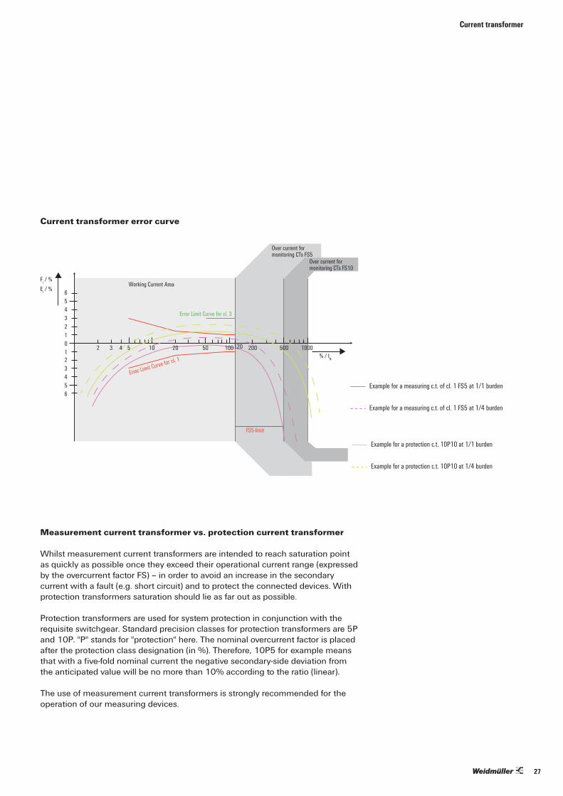
Current transformer error curve

Fi / %

6543210123456

Ei / %

% / IN

2 3 5 50 200

Working Current Area

Over current for monitoring CTs FS5


FS5-limit

Error Limit Curve for cl. 3


Example for a measuring c.t. of cl. 1 FS5 at 1/1 burden


Example for a protection c.t. 10P10 at 1/1 burden


4 10 20 100 500 1000120

Measurement current transformer vs. protection current transformer

Whilst measurement current transformers are intended to reach saturation point as quickly as possible once they exceed their operational current range (expressed by the overcurrent factor FS) – in order to avoid an increase in the secondary current with a fault (e.g. short circuit) and to protect the connected devices. With protection transformers saturation should lie as far out as possible.

Protection transformers are used for system protection in conjunction with the requisite switchgear. Standard precision classes for protection transformers are 5P and 10P. "P" stands for "protection" here. The nominal overcurrent factor is placed after the protection class designation (in %). Therefore, 10P5 for example means that with a five-fold nominal current the negative secondary-side deviation from the anticipated value will be no more than 10% according to the ratio (linear).

The use of measurement current transformers is strongly recommended for the operation of our measuring devices.

Fi / %

6543210123456

Ei / %

% / IN

2 3 5 50 200




FS5-limit







4 10 20 100 500 1000120

Fi / %

6543210123456

Ei / %

% / IN

2 3 5 50 200




FS5-limit







4 10 20 100 500 1000120

Current transformer

27

Rod current transformersType Order No. Round cable Rail Load Accuracy class Primary current Secondary current max.CMA-22-50-5A-1VA-1 2421100000

22.5 mm /

1 VA

1

50 A

5A

CMA-22-60-5A-1.5VA-1 1482140000 1.5 VA 60 ACMA-22-75-5A-1.5VA-1 2421080000 1.5 VA 75 ACMA-22-100-5A-1.5VA-1 2421070000 1.5 VA 100 ACMA-22-150-5A-1.5VA-1 2421060000 1.5 VA 150 ACMA-22-200-5A-2.5VA-1 2421370000 2.5 VA 200 ACMA-22-250-5A-5VA-1 2421050000 5 A 250 ACMA-22-300-5A-5VA-1 2421040000 5 A 300 ACMA-22-400-5A-5VA-0.5 2421010000 5 VA

0.5400 A

CMA-22-500-5A-5VA-0.5 1482220000 5 VA 500 ACMA-22-600-5A-5VA-0.5 1482180000 5 VA 600 A

Plug-on current transformersType Order No. Round cable Rail Load Accuracy class Primary current Secondary current max.CMA-31-60-5A-1.25VA-1 2421380000

25.7 mm20x20 mm25x12 mm30x10 mm

5 A

1

60 A

5A

CMA-31-75-5A-2.5VA-1 1482040000 2.5 VA 75 ACMA-31-100-5A-2.5VA-1 1482030000 2.5 VA 100 ACMA-31-150-5A-5VA-1 2420960000 5 A 150 ACMA-31-200-5A-5VA-1 2420950000 5 A 200 ACMA-31-250-5A-5VA-1 2420940000 5 A 250 ACMA-31-300-5A-5VA-1 2420930000 5 A 300 ACMA-31-400-5A-5VA-1 2420920000 5 A 400 ACMA-31-500-5A-5VA-1 2420910000 5 A 500 ACMA-31-600-5A-5VA-1 2420900000 5 A 600 ACMA-31-750-5A-5VA-1 2420890000 5 A 750 A

Cable-type current converters Type Order No. Round cable Rail Load Accuracy class Primary current Secondary current max.KCMA-18-50-1A-1VA-3 1482020000

18.5 mm

/

1 VA

3

50 A

1A

KCMA-18-75-1A-1VA-3 2420780000 1 VA 75 AKCMA-18-100-1A-1.25VA-3 1482010000 1.25 VA 100 AKCMA-18-150-1A-2VA-3 2420770000 2 VA 150 AKCMA-18-200-1A-3VA-3 2420760000 3 VA 200 AKCMA-18-250-1A-1.5VA-1 1482000000 1.5 VA

1

250 AKCMA-32-400-5A-5VA-1 2420730000

32.5 mm5 VA 400 A

5AKCMA-32-500-5A-5VA-1 2420740000 5 VA 500 AKCMA-32-600-5A-5VA-1 2420720000 5 VA 600 AKCMA-44-750-5A-5VA-1 2420710000 44 mm 5 VA 750 A

Special versionDeviating primary rated current On requestDeviating secondary rated current On requestDeviating construction type On requestDeviating rated frequency On requestExpanded class precision and load durability On requestType-approved / calibrated transformer On request


Current transformer

28

Moulded case feedthrough current transformer

The phase to be measured (conductor rail or line) is fed through the CT window and forms the primary circuit for the current transformer. Feedthrough transformers are predominantly used for mounting on bus bars. Through additional potting it is possible to achieve droplet-tightness, as well as greater shock and vibration resistance with mechanical loading (IEC 68). This is the most common form of current transformers, with the disadvantage that the primary conductor must be interrupted during installation. This form of transformer is therefore most commonly used in new system installations.

Split core current transformer

Split core current transformers are frequently used with retrofit applications. With these transformers the transformer core is open ready for installation, and is therefore fitted around the bus bars. This enables installation without interrupting the primary conductor.

Cable type split core current transformer

Cable type split core current transformers are exclusively suitable for installation in isolated primary circuit conductors (supply cables) in weatherproof and dry locations. Installation is possible without interrupting the primary conductor (i.e. with ongoing operation).

Current transformer construction types

Current transformer

Cable-type current converters

29

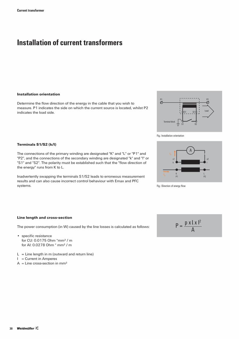
Installation orientation

Determine the flow direction of the energy in the cable that you wish to measure. P1 indicates the side on which the current source is located, whilst P2 indicates the load side.

Terminals S1/S2 (k/l)

The connections of the primary winding are designated "K" and "L" or "P1" and "P2", and the connections of the secondary winding are designated "k" and "l" or "S1" and "S2". The polarity must be established such that the "flow direction of the energy" runs from K to L.

Inadvertently swapping the terminals S1/S2 leads to erroneous measurement results and can also cause incorrect control behaviour with Emax and PFC systems.

Line length and cross-section

The power consumption (in W) caused by the line losses is calculated as follows:

• specific resistance for CU: 0.0175 Ohm *mm² / m for AI: 0.0278 Ohm * mm² / m

L = Line length in m (outward and return line)I = Current in AmperesA = Line cross-section in mm²

Installation of current transformers

P1 P2

S1 S2

S1 S2

Load

Terminal block

Isn

Ipn

A

s2s1k I

KP1

LP2

Energieflussrichtung

Fig.: Installation orientation

Fig.: Direction of energy flow

P = p x x I2A

Current transformer

30

Brief overview (power consumption copper line) for 5 A and 1 A:

With every temperature change of 10 °C the power consumed by the cables increases by 4 %.

Power consumption in VA at 5 ANominal cross-section 1 m 2 m 3 m 4 m 5 m 6 m 7 m 8 m 9 m 10 m

2.5 mm² 0.36 0.71 1.07 1.43 1.78 2.14 2.50 2.86 3.21 3.574.0 mm² 0.22 0.45 0.67 0.89 1.12 1.34 1.56 1.79 2.01 2.246.0 mm² 0.15 0.30 0.45 0.60 0.74 0.89 1.04 1.19 1.34 1.49

10.0 mm² 0.09 0.18 0.27 0.36 0.44 0.54 0.63 0.71 0.80 0.89

Power consumption in VA at 1 ANominal cross-section 10 m 20 m 30 m 40 m 50 m 60 m 70 m 80 m 90 m 100 m

1.0 mm² 0.36 0.71 1.07 1.43 1.78 2.14 2.50 2.86 3.21 3.572.5 mm² 0.14 0.29 0.43 0.57 0.72 0.86 1.00 1.14 1.29 1.434.0 mm² 0.09 0.18 0.27 0.36 0.45 0.54 0.63 0.71 0.80 0.896.0 mm² 0.06 0.12 0.18 0.24 0.30 0.36 0.42 0.48 0.54 0.60

10.0 mm² 0.04 0.07 0.11 0.14 0.18 0.21 0.25 0.29 0.32 0.36

Example of current transformer capacity and line lengthSecondary current = 1 ALine = 0.75 mm²Current transformer capacity / line length

Secondary current = 5 ALine = 2.5 mm²Current transformer capacity / line length

Class 0.5 Class 1 Class 3 Class 0.5 Class 1 Class 30.5 VA / 5 m 0.5 VA / 5 m 0.25 VA / 1 m 0.5 VA / 0.7 m 0.5 VA / 0.7 m 0.5 VA / 0.7 m1 VA / 15 m 1 VA / 15 m 0.5 VA / 5 m 1 VA / 2.1 m 1 VA / 2.1 m 1.5 VA / 3.5 m2.5 VA / 47 m 1.5 VA / 26 m 1 VA / 15 m 2.5 VA / 6 m 2.5 VA / 6 m 2.5 VA / 6 m5 VA / 100 m 2.5 VA / 47 m 1.5 VA / 26 m 5 VA / 13 m 5 VA / 13 m10 VA / 205 m 5 VA / 100 m 10 VA / 27 m

10 VA / 200 m 20 VA / 55 m20 VA / 400 m

Serial connection of measuring devices to a current transformer

Pv = Measuring device 1 + Measuring device 2 +….+ PLine + PTerminals ….?

Current transformer

31

Operation in parallel / summation current transformer

If the current measurement is carried out via two current transformers, the overall transformer ratio of the current transformers must be programmed into the measuring device.

Example: Both current transformers have a transformer ratio of 1,000/5A. The total measurement is carried out using a summation current transformer 5+5 / 5 A.

The UMG must then be set up as follows:

Primary current: 1,000 A + 1,000 A = 2,000 ASecondary current: 5 A

Grounding of current transformers

According to VDE 0414, current and voltage transformers should be secondary grounded from a series voltage of 3.6 kV. With low voltage it is possible to dispense with grounding if the current transformers do not possess large metal contact surfaces. However, common practice is to ground low voltage transformers too. Customary is grounding on S1. However, grounding can also take place on the S1(k) terminal or S2(k) terminals. Important: Always ground on the same side!

Use of protection current transformers

In the event of retrofitting a measuring device and the exclusive availability of a protective core, we recommend the use of a winding current transformer 5/5 for decoupling the protective core.

Power supplyvoltage

Ethe

rnet

10/1

00Ba

se-T

PC

Measuring voltage

RJ45

Current measurement

V1 V2 V3 VN

3 4 5 61 2N/- L/+

S2 S1

S2

S2

S1

S1 L1L2L3Lo

ads

230V/400V 50HzN

S2 S1 S2 S1 S2 S1I3 I2 I1

12 11 10 9 8 7

Energy Meter 525

Abb.: Energy Analyser 550 Current measurement via summation transformer

Fig.: Connection example Energy Meter 525

Consumer A Consumer B

1P1(K)

(L) 1P2

2P1(K)

(L) 2P2

1S1

(k)(l)

1S2

(k) S1

2S1

(k)(l)

2S2

Supply 1 Supply 2S2 (l)

BLAK AL BK

19 20I1

Energy Analyser 550

Current transformer

Installation of current transformers

32

Exchanging a measuring device (short-circuiting of current transformers)

The current transformer secondary circuit should never be opened when current is flowing into the primary circuit.

The current transformer output constitutes a current source. With an increasing burden the output voltage therefore increases (according to the relationship U = R x I) until saturation is reached. Above saturation point the peak voltage continues to rise with increasing distortion, and attains its maximum value with an endless burden, i.e. open secondary terminals. With open transformers it is therefore possible that voltage peaks may arise, which could pose a risk of danger to persons and may also destroy measuring devices when reconnected.

It is therefore the case that open operation of CTs must be avoided and unloaded current transformers must be short circuited.

Current transformer terminal block with short circuit devices

In order to short circuit current transformers and for the purpose of recurrent comparative measurements it is recommended that special terminal block for DIN rails be used. These comprise a cross-disconnect terminal with measuring and test equipment, insulated bridges for grounding and short circuiting of the current transformer terminals.

Overloading of measurement CTs

Primary current overloading:Primary current too high --> Saturation of the core material --> Precisiondeclines dramatically.

Nominal power overloading:Too many measuring devices or excessively long lines are connected to a transformer with its defined nominal power --> Saturation of the core material --> Precision declines dramatically.

Instance of short circuit at CT secondary side

In the event of a short circuit no signal is available. It is not possible to measurewith the measuring device. Current transformers can (or must) be short circuited if no load is present (measuring device).

Fig.: Current transformer terminal block

Operation of current transformers

Current transformer

33

If it is necessary to network economical measuring devices with each other, the RS485 interface with Modbus RTU protocol remains the benchmark. The simple topology configuration, the lack of sensitivity to EMC interference and the open protocol have been outstanding features of the combination of RS485 and Modbus RTU protocol for years. The full name of the RS485 standard is TIA / EIA-485-A. The most recent update was in March 1998 and the standard was confirmed in 2003 without changes. The standard only defines the electrical interface conditions of the sender and receiver, it does not say anything about the topology or the lines to be used. This information can either be found in the TSB89 "Application Guidelines for TIA / EIA-485-A" or in the application descriptions of the RS485 driver module manufacturers, such as Texas Instruments or Maxim. According to the OSI model (Open Systems Interconnection Reference Model)* only the "physical layer" and not the protocol is described. The protocol used may be selected on an arbitrary basis, e.g. Modbus RTU, Profibus, BACnet etc. The communication between the sender and receiver takes place on a wired basis via shielded, twisted pair cable. One cable pair should only ever be used here for A and B (Fig.: Image 1b). If the interface is not galvanically separated then the common connection must also be routed with it (Fig.: Image 1b). More on this later.

The transfer of data takes place via a differential, serial voltage signal between lines [A] and [B]. Because data is transferred on the lines between sender and receiver, one also refers here to half-duplex or alternating operation. Each receiver or sender has an inverted and a non-inverted connection. The data transfer takes place symmetrically. This means that if one line has a "high" signal then the other has a "low" signal. Line A is therefore complementary to B and vice versa. The advantage of measuring the voltage difference between A and B is that common mode interference has largely no influence. Any common mode interference is coupled on both signal lines approximately equally, and due to the differential measurement it therefore has no influence on the data that is to be transferred. The sender (driver) generates a differential output voltage of at least 1.5 V at 54 Ohm load. The receiver has a sensitivity of +/-200 mV (Fig. Image 2).

The state logic here is as follows (Fig. Image 3):

A–B < 0,25 V = Logic 1A–B > 0,25 V = Logic 0

The labelling of connections A / B is often not uniform. What is A with one manufacturer, may be B with the next. Why is this the case?

* Open Systems Interconnection Reference Model (OSI): Driver = Sender; Receiver = Recipient; Transceiver = Sender / Receiver

Communication via the RS485 interface

Fig.: Image 1

R

D

C

AB

+200 mV –200 mV

+1,5 V –1,5 V

B

A

5050

2,502,5

AB

1 0 1 1 0 1 0 1 1 0 1 1

t

t

VA–VBMath

①

②

③

Fig.: Image 2

Fig.: Image 3

Fig.: Image 1a

A A

A A

B B

B B

C* C*

A A

A A

B B

B B

C* C*

Fig.: Image 1b


34

The definition says:

A = “-“ = T x D- / R x D - = inverted signalB = “+“ = T x D + / R x D + = non-inverted signal

Furthermore, a third line "C" = "Common" is also cited.This line is for the reference ground.

However, some RS485 chip manufacturers such as Texas Instruments, Maxim,Analog Devices etc. have always used an alternative designation, which hassince also become commonplace:

A = “+“ = T x D + / R x D + = non-inverted signalB = “-“ = T x D - / R x D - = inverted signal

Due to this confusion, some device manufacturers have introduced their owndesignations:

D+ = “+“ = T x D + / R x D + = non-inverted signal D- = “-“ = T x D - / R x D - = inverted signal

Through the [+] and [-] sign after the letter [D] it is clear which line is providingthe inverted and the non-inverted signal.

All of our measuring devices utilise the following designations:

A = “+“ = T x D + / R x D + = non-inverted signal B = “-“ = T x D - / R x D - = inverted signal

The voltages are defined in the datasheets as follows:

A

BD

C

VO

VOB VOS VOA

Fig.: Image 4

VO = Differential voltage A – BVOB = Voltage between B and CVOA = Voltage between A and CVOS = Driver offset voltage


35

The voltage VCM

The voltage VCM (Common Mode Voltage) is the sum of the GND potential differences between the RS485 participants (Fig.: Image 5), the driver offset voltage and the common mode noise (Vnoise), acting on the bus line. The RS485 driver manufacturers give a voltage range for VCM of -7 to 12 V. With communication problems, this voltage range - resulting from the potential differences between sender and receiver - is frequently impeded if the interface is not galvanically separated by configuration or no common line exists. Image 6 shows the calculation of the common mode voltage.

+12

–7

0B

A

Common-mode Voltage

Fig.: Image 5

Master A

BD

CVOBVOS

VOA

VGPD

R

Vnoise Slave

Fig.: Image 6

VGPD (Ground potential differences)

VGPD is the potential difference between sender and receiver here GND (PE). Potential differences between the connections (grounding) often arise with larger spatial expansion of the RS485 bus. These potential differences arise in particular with older electrical installations, because no intermeshed potential equalisation exists in many cases. Furthermore, the effects of lightening result in the potential difference between the PE connections in the distribution system approaching hundreds or thousands of volts. It is also possible under normal conditions that potential differences of a few volts may exist due to the equalisation currents of

VOS =VOA + VOB

2

VCM = VOS + Vnoise + VGPD



36

the loads. Vnoise (common mode noise) is an interference voltage that can have the following causes: V

• Interference voltage induced by a magnetic field on the bus line

Magnetic fieldMaster

750

D370 D370 D370

M

Fig.: Image 7

• Capacitive coupling with system parts that are not galvanically separated ("parasitic capacities")

Master

M

Erde

Slave Slave

Fig.: Image 8

• Galvanic coupling• Radiant coupling• Electrostatic discharge


37

Bus topology

The bus is "multipoint-capable" and it is possible to connect up to 32 participants without a repeater. The best network topology here is the "daisy chain". This means that the bus cable runs directly from slave to slave.

Master AB

Slave Slave Slave... 32

Fig.: Image 9

It is necessary to note that stub lines (branches) should be avoided in general. Stub lines cause reflections on the bus. In theory it is feasible to calculate a possible stub line depending on the transceiver used. However, this is complex in practice. The length of a possible stub line is heavily dependent on the signal rise time of the transceiver used and should be less than 1/10 of the signal rise time of the driver. The higher the possible Baud rate of the transceiver, the smaller the signal rise time of the driver. This means one must know which IC has been installed with the bus participants. Furthermore, the signal speed of the cable must also be applied in the calculation. For this reason, one should avoid stub lines in general..

Termination

A further cause of communication interruptions are bus reflections. A reflection arises if the sender signal has not been fully absorbed by the load. The source impedance should reflect the load impedance and the line surge impedance, because the full signal power is attained through this and only minimum reflections arise. Serial communication of the RS485 interface functions most efficiently when the source and load impedance are harmonised at 120 Ohm. For this reason, the RS485 standard recommends a bus line with a line surge impedance of Z0 = 120 Ohm. In order that reflections are avoided on the bus, the bus line must be equipped with a termination resistor at the start and end, and this must reflect the line surge impedance..



38

Master

Slave Slave Slave

120 Ohm

Zo =120 Ohm

120 Ohm

Fig.: Image 10

“Failsafe Bias” resistors

If the receiver inputs fall within the range of -200 mV to + 200 mV, the output of the receiver module is undetermined, i.e. it is not possible for an evaluation of the RS485 signal to take place.

This is the case under the following conditions:

• No sender active• The bus line has been interrupted (e.g. line break)• The bus line has short circuited (e.g. line damaged, etc.)

Under these conditions the RS485 bus must be brought to a defined signal status. Some communication buses do not have this problem because only one sender exists for example, which controls the line. The sender is either active or inactive. However because the RS485 bus is multipoint-capable, multiple senders can be connected.

In order that the signal status is clear under the aforementioned conditions, one generally uses a "pull up" resistor between +5 V and the signal line A and a "pull down" resistor between GND and signal line B. The resistors can theoretically be placed at an arbitrary point in the bus. However, these are generally used with a master in a potential divider group with termination resistor because readily assembled connectors exist for this purpose.

With some manufacturers one generally only finds a recommendation to install a termination resistor at the start and end, in order that reflections can be avoided. Why is this the case?

In this case the manufacturers have used transceivers for the RS485 interface, which already have an integrated internal Failsafe Bias in the chip, i.e. with 0 V at the receiver input for example, the output automatically has a logical "High" state. With Maxim (as used in the UMG 604 and UMG 103) the function is called "True


39

fail-safe". An external Failsafe Bias then only remains necessary if participants are connected to the same bus, which do not possess this function. The bus load is otherwise unaffected by the "True fail-safe" function.

The “common connection” or “galvanic separation”

The bus participants generally obtain their supply voltage from different areas of the electrical installation. With older electrical installations in particular, it is therefore possible that considerable potential differences can arise between grounding. However, for fault-free communication the voltage Vcm can only lie within the range of -7 to +12 V, i.e. the voltage VGPD (Ground potential differences) must be as small as possible (image 11 a, image 5). If the RS485 interface is not galvanically separated from the supply voltage then the common connection must be routed with it (image 11 b). However, connection with the common connections may result in a current loop, i.e. without additional measures a higher compensation current will flow between the bus participants and ground. Developers generally prevent this by decoupling the GND of the RS485 interface from the ground with a 100-Ohm resistor (image 11 c).

A better alternative is the galvanic separation of the RS485 interface from the supply voltage through an internal DC/DC converter and a signal isolator. This means that potential differences in the ground have no effect on the signal. The differential signal therefore "floats". Even better still is the galvanic separation of the RS485 interface in combination with a common connection.

Image 12 shows mixed operation between participants of galvanically separated and non-galvanically separated interfaces. The participants with the galvanically separated RS485 have no common connection in the example. In this case it is necessary to ensure that the common connections of the participants are connected with each other. Despite this, communication interferences can arise due to EMC coupling capacitors. This results in the non-galvanically separated participants no longer being able to interpret the signal. In this case the bus must be separated and an additional galvanic coupling must be integrated between the participant circuits.



40

VCC1 VCC2 VCC3 VCC4

A B A B A B A B

C C

Isolation Isolation

VCC1 VCC2

GPD

A B A BC C

Vn

VCC1 VCC2

A B A B

GND GND

high current

VCC1 VCC2

A B A B

GND GND100 Ohm 100 Ohm

low current

DC/DC Converter

Signal Isolator

GND

Ⓐ

Ⓑ

Ⓒ

Ⓓ

VCC1 VCC2

GPD

A B A BC C

Vn

VCC1 VCC2

A B A B

GND GND

high current

VCC1 VCC2

A B A B

GND GND100 Ohm 100 Ohm

low current

DC/DC Converter

Signal Isolator

GND

Ⓐ

Ⓑ

Ⓒ

Ⓓ

Fig.: Image 11

Fig.: Image 12

Note: The screening must never be connected to the common connection of the RS485 interface. This would result in faults being directly coupled with the GND of the RS485 transceiver.


41

Ports, protocols and connections

Energy Analyser D550, Energy Analyser 550Protocols PortsTFTP 1201Modbus / TCP – Modbus / UDP 502, 4 PortsDHCP 68NTP 123BACnet 47808Nameservice 1200HTTP 80FTP 21FTP data port 1024, 1025FTP data port 1026, 1027Modbus over Ethernet 8000, 1 PortService port (telnet) 1239SNMP 161 / 162 (TRAP)E-Mail port (actual) 25E-Mail port (in preparation) 587

ecoExplorer goProtocols PortsModbus / TCP – Modbus / UDP 502HTTP 80FTP 21FTP data port 1024, 1025FTP data port 1026, 1027Modbus / TCP 502Modbus over Ethernet 8000Read out telnet data port 1239Update telnet data port 1236, 1237E-Mail port (in preparation) 25E-Mail port (in preparation) 587

Energy Meter D370, Energy Meter D650Protocols PortsThe devices do not have anEthernet connection

The devices do not have anEthernet connection


Number of TCP/UTP connections (Energy Analyser D550, Energy Analyser 550) • A max. total of 24 connections are possible via the TCP group.

The following applies: – Port 21 (FTP): max. 4 connections – Port 25/587 (E-Mail): max. 8 connections – Port 1024-1027 (data port to every FTP port): max. 4 connections – Port 80 (HTTP): max. 24 connections – Port 502 (Modbus TCP/IP): max. 4 connections – Port 1239 (Debug): max. 1 connection – Port 8000 (Modbus or TCP/IP): max. 1 connection

• Connection-free communication via the UTP group

– Port 68 (DHCP) – Port 123 (NTP) – Port 161/162 (SNMP) – Port 1200 (Nameservice) – Port 1201 (TFTP)

Fig.: TCP group: max. 24 connections (queue scheduling) (Energy Analyser D550, Energy Analyser 550)

Port 80(HTTP)

max. 24 connections

Port 502(Modbus TCP/IP)

(also fot slave)

max. 4 connections

Port 21(FTP)

max. 4 connections

Port 25/587Email

max. 8 connections

Port 1024-1027(One FTP port requires

a data port)max. 4 connections

Port 8000E-(Modbus or TCP/IP)

max. 1 connection

Port 1239(Debug)

max. 1 connection

42

The Energy Meter 750 supports the following protocols via Ethernetconnection

Client services PortsDNS 53 (UDP / TCP)DHCP-Client (BootP) 68 (UDP)NTP (Client) 123 (UDP)E-Mail (sending) Selectable (1-65535 TCP)

Server services PortPing (ICMP / IP)FTP 20 (TCP)*, 21 (TCP)HTTP 80 (TCP)NTP (only listen) 123 (UDP Broadcast)SNMP 161 (UDP)Modbus TCP 502 (UDP / TCP)Device identification 1111 (UDP)Telnet 1239 (TCP)Modbus RTU (Ethernet encapsulated) 8000 (UDP)

* Random port (> 1023) for data transfer, if work is taking place in PASSIVE mode

The Energy Meter 750 can administrate 20 TCP connections.

Client services are contacted by a device on a server via the specified ports,the server services make the device available.

Fig.: UTP group: Connection-free communication (Energy Analyser D550, Energy Analyser 550)

Port 68 (DHCP)

Port 123 (NTP)

Port 161/162 (SNMP)

Port 1200 (Nameservice)

Port 1201 (TFTP)

Port 47808 (BACnet)


43

Electrical distribution systems and loads are becoming increasingly complex. This also results in the likelihood of transient overvoltage increasing. Power electronic modules in particular (e.g. frequency converters, phase angle and trailing-edge control, PWM-controlled power switches) generate temporary voltage peaks in conjunction with inductive loads, which can be significantly higher than the respective nominal voltage. In order to guarantee user safety, four overvoltage categories (CAT I to CAT IV) are defined in DIN VDE 0110 / EN 60664.

The measurement category indicates the permissible application ranges of measuring and test devices for electrical operating equipment and systems (e.g. voltage testers, multimeters, VDE test devices) for application in low voltage network areas.

Defined categories and application purposes in IEC 61010-1:The following categories and application purposes are defined in IEC 61010-1:

CAT IMeasurements on current circuits that have no direct connection to the mains network (battery operation), e.g. devices in protection class 3 (operation with protective low voltage), battery-operated devices, car electrics

CAT IIMeasurements on current circuits that have a direct connection by means of a plug with the low voltage network, e.g. household appliances, portable electrical appliances

CAT IIIMeasurements within the building installation (static loads with direct fixed connection, distribution connection, fixed installation appliances in the distribution system), e.g. sub-distribution.

CAT IVMeasurements at the source of the low voltage installation (meter, main connection, primary overcurrent protection), e.g. revenue meters, low voltage overhead lines, utility service entrance box

Additionally categories are divided in the voltage levels 300 V / 600 V / 1.000 V.

The category is particularly significant for safety during measurements, because low-resistance current circuits exhibit higher short circuit currents and / or the measuring device is also required to withstand disturbances in the form of load switching and other transient overvoltages, without the user being endangered by electric shocks, fire, sparks forming or explosions. Due to the low impedance of the public grid, short circuit currents are at their g reatest at the house infeed. Inside the home, the maximum short circuit currents are reduced through the system's series impedances. Technically, compliance with the category is ensured for example through the contact protection of plugs and sockets, insulation, sufficient clearance and creepage distances, the strain relief and kink protection of cables, as well as sufficient cable cross-sections.

Overvoltage categories


44

In practice

Our experience and understanding shows that many users are not sufficiently familiar with this subject. In some applications, the subject of overvoltage categories may result in a need to change from a Energy Analyser D550 with 300 V CAT-III to a Energy Analyser 550 with the overvoltage category 600 V CATIII, i.e. instead of a 4,000-V measurement voltage surge, a 50 % higher measurement voltage surge of 6,000 V is attained! However, it may also result in the shifting of the measurement point. This means additional safety for man and machine!

The combination of the CAT category and the defined voltage level givesthe measurement voltage surge.

Rated voltages of power supply systems (networks) with various types of overvoltage limitationVoltage conductor to neutral conductor, taken from rated AC voltage or rated DC voltage up to and including

V

Rated voltages presently in use worldwide Measurement voltage surgefor operating equipment

Three-phase 4-conductorsystems withgrounded neutral conductor

V

Three-phase 3-conductorsystems, ungrounded

V

Single-phase 2-conductorsystems, AC or DC voltage

V

Single-phase 3-conductorsystems, AC or DC voltage

VOvervoltage categories I II III IV

150120 / 208*127 / 220

115, 120, 127100**110, 220

100 – 200**101 – 220120 – 240

800 1,500 2,500 4,000

300220 / 380, 230 / 400 240 / 415, 260 / 440 277 / 480

200**, 220, 230, 240, 260, 277, 347, 380, 400, 415, 440

220 220 – 400 1.500 2,500 4,000 6,000

600347 / 600, 380 / 660 400 / 690, 417 / 720

500 480 480 – 960 2.500 4,000 6,000 8,000

* Conventional in the United States of America and Canada.** Conventional in Japan.

E


45

Weidmüller devices are developed, produced and tested according to internationally valid standards and directives. The most important national and international standards in conjunction with our products, solutions and applications are as follows:

General standards and EMC standards:

• IEC/EN 61000-2-2: Electromagnetic compatibility (EMC): Ambient conditions; compatibility level for low frequency, conducted interferences and signal transferral in public low voltage networks.

• IEC/EN 61000-2-4: Electromagnetic compatibility (EMC): Ambient conditions; compatibility level for low frequency, conducted interferences in industrial plants.

• IEC/EN 61000-3-2: Threshold values for harmonic currents for electrical devices with current consumption of < 16 A per phase.

• IEC/EN 61000-3-3: Threshold values – limit of voltage changes, voltage variations and flicker in public low voltage supply networks for devices with a rated current ≤16 A per phase..

• IEC/EN 61000-3-4: Electromagnetic compatibility (EMC): Threshold values limit of transmission of harmonic currents in low voltage supply networks for devices and equipment with rated currents of over 16 A.

• IEC/EN 61000-3-11: Electromagnetic compatibility (EMC): Threshold values – limit of voltage changes, voltage variations and flicker in public low voltage supply networks; devices and equipment with a rated current ≤ 75 A.

• IEC/EN 61000-3-12: Threshold values for harmonic currents, caused by devices and equipment with a current input of > 16 A and ≤ 75 A per phase, which are intended for connection with public low voltage networks.

• IEC/EN 61557-12: Electrical safety in low voltage networks up to AC 1000 V and DC 1500 V – Devices for testing, measuring or monitoring protective measures.

Valid standards

Power quality standards:

• EN 50160: Characteristics of the voltage (PQ) in public electricity supply networks.

• D-A-CH-CZ: Technical regulations for the evaluation of grid distortion effects in Germany, Austria, Switzerland and the Czech Republic.

• TOR D2: Technical and organisational regulations for operators and users of electrical networks, Part D: Special technical regulations; section D2: Directives for the evaluation of grid distortion effects.

• IEEE 519: (Recommended Practices and Requirements for Harmonics Control in Electrical Power Systems) as a common recommendation from energy suppliers and operators for limiting the effects of non-linear loads through the reduction of harmonics.

• ENGINEERING RECOMMENDATION: G5/4-1 (planning levels for harmonic voltage distortion to be used in the process for the connection of non-linear equipment) as a directive of the Energy Networks Association (UK) for limiting the effects of non-linear loads through the reduction of harmonics at the transition point (PCC). Valid in Great Britain and Hong Kong.

• IEEE1159-3 PQDIF: Recommended Practice for the Transfer of Power Quality Data (data exchange format for power quality data).

• ITIC (CBEMA): The ITI curve of the Information Technology Industry Council (ITI) represents the withstand capability of computers / power supplies in relation to the height and duration of voltage variations.

Standards for power quality analysers

• IEC/EN 61000-4-2: Electromagnetic compatibility (EMC) – Part 4-2: Testing and measurement techniques – Electrostatic discharge immunity test.

• IEC/EN 61000-4-3: Electromagnetic compatibility (EMC)Part 4-3: Testing and measurement techniques – Radiated, radio-frequency, electromagnetic field immunity test.

Valid standards

46

• IEC/EN 61000-4-4: Electromagnetic compatibility (EMC) – Part 4-4:Testing and measurement techniques – Electrical fast transient/burst immunity test.

• IEC/EN 61000-4-5: Electromagnetic Compatibility (EMC) – Part 4-5: Testing and measurement techniques – Surge immunity test.

• IEC/EN 61000-4-6: Electromagnetic compatibility (EMC)Part 4-6: Testing and measurement techniques – Immunity to conducted disturbances, induced by radio-frequency fields.

• IEC/EN 61000-4-7: Electromagnetic compatibility (EMC) – Part 4-7: Testing and measurement techniques – General guide on harmonics and interharmonics measurements and instrumentation, for power supply systems and equipment connected thereto.

• IEC/EN 61000-4-8: Electromagnetic compatibility (EMC) – Part 4-8: Testing and measurement techniques – Power frequency magnetic field immunity test.

• IEC/EN 61000-4-11: Electromagnetic compatibility (EMC) – Part 4-11: Testing and measurement techniques – Voltage dips, short interruptions and voltage variations immunity tests.

Standards for energy measurement devices

• DIN EN 62053-21: Electricity metering equipment (a.c.) – Particular Requirements – Part 21: Static meters for active energy (classes 1 and 2).

• DIN EN 62053-22: Electricity metering equipment (a.c.) – Particular requirements – Part 22: Static meters for active energy (classes 0,2 S and 0,5 S).

• DIN EN 62053-23: Electricity metering equipment (a.c.) – Particular requirements – Part 23: Static meters for reactive energy (classes 2 and 3).

• DIN EN 62053-31: Electricity metering equipment (a.c.) – Particular requirements – Part 31: Pulse output devices for electromechanical and electronic meters (two wires only.

• DIN EN 60529: Degrees of protection provided by enclosures (IP code).

Standards for energy management

• DIN ISO 50001: Energy management systems – Requirements with instructions on application.

• DIN EN 16247: Describes the requirements for an energy audit, which enables small and medium-sized companies (SME) to improve their energy efficiency and reduce their energy consumption.

• DIN EN 16247-1: Energy audits – Part 1: General requirements; possibility for small and medium-sized companies (SME), in the sense of recommendation 2003/361/EC of the European Commission, to fulfil the requirements of the electricity and energy tax legislation for surplus settlement.

Valid standards

47

Notes

48

Made in Germany/04/2016/SMKW

Weidmüller – Your partner in Industrial Connectivity

As experienced experts we support our customers and partners around the worldwith products, solutions and services in the industrial environment of power,signal and data. We are at home in their industries and markets and know thetechnological challenges of tomorrow. We are therefore continuously developinginnovative, sustainable and useful solutions for their individual needs. Together weset standards in Industrial Connectivity.

Your local Weidmüller partner canbe found on our website:www.weidmueller.com/countries

Weidmüller Interface GmbH & Co. KGKlingenbergstraße 1632758 Detmold, GermanyT +49 5231 14-0F +49 5231 [email protected]

Documents

Energy management - Basic knowledge Technical Information