Energy Efficient Routing Protocols in

Wireless Sensor Network

Thesis submitted in fulfillment of the requirement for the degree of

Masters of Technology (Hons.) in

Computer Science and Engineering

By Pawan Singh Faujadar Roll No.: 03CS3006

Under the supervision of Prof. Niloys Ganguly

Department of Computer Science and Engineering Indian Institute of Technology

Kharagpur – 721302 INDIA

2

Certificate This is to certify that the report titled Energy Efficient Routing Protocols in Wireless Sensor Networks submitted by Pawan Singh Faujadar to the Department of Computer Science and Engineering, in fulfillment for the award of the degree Masters of Technology, is a bona-fide record of work carried out by him under my supervision and guidance. The report has fulfilled all the requirements as per the regulations of this institute, and in my opinion has reached the standard needed for submission.

Professor Niloy Ganguly Computer Science & Engineering Department

Indian Institute of Technology – Kharagpur INDIA

3

Acknowledgements I am greatly indebted to my project supervisor Prof. Niloy Ganguly for inspiring and motivating me to develop ideas and implementing them. I am grateful to him for his invaluable guidance and encouragement for the project. I would like to take this opportunity to express my sincere and profound gratitude to him for the pains he has taken for the project.

Pawan Singh Faujadar Computer Science & Engineering Department

Indian Institute of Technology – Kharagpur INDIA

4

Index: Page No.

1. Abstract 5

2. Introduction 6

3. Problem Formulation 9

4. Placement & Localization 10

5. Routing Protocols 14

6. Sensor Network Simulator 24

7. Results 27

8. Conclusion 35

9. References 36

5

1. Abstract One of the limitations of wireless sensor nodes is their inherent

limited energy resource. Besides maximizing the lifetime of the

sensor node, it is preferable to distribute the energy dissipated

throughout the wireless sensor network in order to minimize

maintenance and maximize overall system performance. Any

communication protocol that involves synchronization of peer nodes

incurs some overhead for setting up the communication. So here we

study various energy-efficient routing algorithms and compare

among themselves. We take into account the setup costs and analyze

the energy-efficiency and the useful lifetime of the system. In order

to better understand the characteristics of each algorithm and how

well they really perform, we also compare them with an optimum

clustering algorithm.

The benefit of introducing these ideal algorithms is to show

the upper bound on performance at the cost of an astronomical

prohibitive synchronization costs. We compare the algorithms in

terms of system lifetime, power dissipation distribution, cost of

synchronization, and simplicity of the algorithm.

6

2. Introduction

Over the last half a century, computers have exponentially increased

in processing power and at the same time decreased in both size and

price. These rapid advancements led to a very fast market in which

computers would participate in more and more of our society’s daily

activities. In recent years, one such revolution has been taking place,

where computers are becoming so small and so cheap, that single-

purpose computers with embedded sensors are almost practical from

both economical and theoretical points of view. Wireless sensor

networks are beginning to become a reality, and therefore some of

the long overlooked limitations have become an important area of

research.

In our project, we attempt to find out and overcome

limitations of the wireless sensor networks such as: limited energy

resources, varying energy consumption based on location, high cost of

transmission, and limited processing capabilities. All of these

characteristics of wireless sensor networks are complete opposites of

their wired network counterparts, in which energy consumption is not

an issue, transmission cost is relatively cheap, and the network nodes

have plenty of processing capabilities. Routing approaches that have

worked so well in traditional networks for over twenty years will not

suffice for this new generation of networks.

Besides maximizing the lifetime of the sensor nodes, it is

preferable to distribute the energy dissipated throughout the wireless

sensor network in order to minimize maintenance and maximize

overall system performance. Any communication protocol that

involves synchronization between peer nodes incurs some overhead of

7

setting up the communication. So here, we attempt determine

whether the benefits of more complex routing algorithms overshadow

the extra control messages each node needs to communicate. Each

node could make the most informed decision regarding its

communication options if they had complete knowledge of the entire

network topology and power levels of all the nodes in the network.

This indeed proves to yield the best performance if the

synchronization messages are not taken into account. However, since

all the nodes would always need to have global knowledge, the cost of

the synchronization messages would ultimately be very expensive.

For both the diffusion and clustering algorithms, we will analyze both

realistic and optimum schemes in order to gain more insight in the

properties of both approaches.

The usual topology of wireless sensor networks involves

having many network nodes dispersed throughout a specific physical

area. There is usually no specific architecture or hierarchy in place

and therefore, the wireless sensor networks are considered to be ad

hoc networks. An ad hoc wireless sensor network may operate in a

standalone fashion, or it may be connected to other networks, such as

the larger Internet through a base station. Base stations are usually

more complex than mere network nodes and usually have an

unlimited power supply. Regarding the limited power supply of

wireless sensor nodes, spatial reuse of wireless bandwidth, and the

nature of radio communication cost which is a function of the distance

transmitted squared, it is ideal to send information in several smaller

hops rather than one transmission over a long communication

distance.

In our simulation, we use a data collection problem in which

the system is driven by rounds of communication, and a sensor node

8

has a packet to send to the distant base station if it detects a target

within its sensing radius. The algorithms are mainly based on location,

power levels, and load on the node, and their goal is to achieve better

target sensing with minimizing the power consumption and

maintenance throughout the network so that the majority of the

nodes consume their power supply at relatively the same rate

regardless of physical location. This leads to better maintainability of

the system, such as replacing the batteries all at once rather than one

by one, and maximizing the overall system performance by allowing

the network to function at 100% capacity throughout most of its

lifetime instead of having a steadily decreasing node population.

9

3. Problem Formulation

Task is to study, simulate and compare various routing algorithms

used in Wireless Sensor Networks, clubbed with some placement

algorithms such that they can address the following problem:

Given a remote rectangular field, the task is establish a sensor

network, having its base station at centre, with some sensor node

placement and following a certain routing protocol, such that it can

monitor fixed or randomly generated targets and report the targets to

the base station, consuming less power & maintenance and

without compromising with the performance.

10

4. Placement & Localization of sensor nodes:

Here, let us first discuss some placements and localization techniques

considered in our experiment:

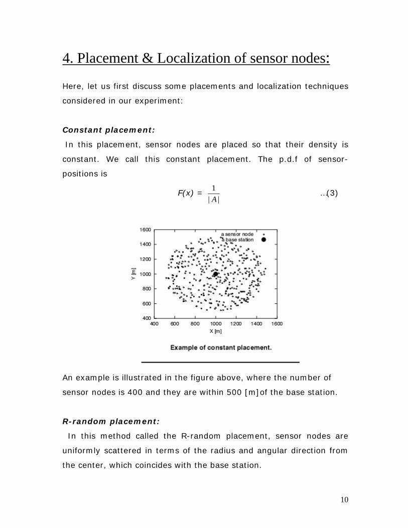
Constant placement:

In this placement, sensor nodes are placed so that their density is

constant. We call this constant placement. The p.d.f of sensor-

positions is

F(x) = 1

| |A …(3)

An example is illustrated in the figure above, where the number of

sensor nodes is 400 and they are within 500 [m]of the base station.

R-random placement:

In this method called the R-random placement, sensor nodes are

uniformly scattered in terms of the radius and angular direction from

the center, which coincides with the base station.

11

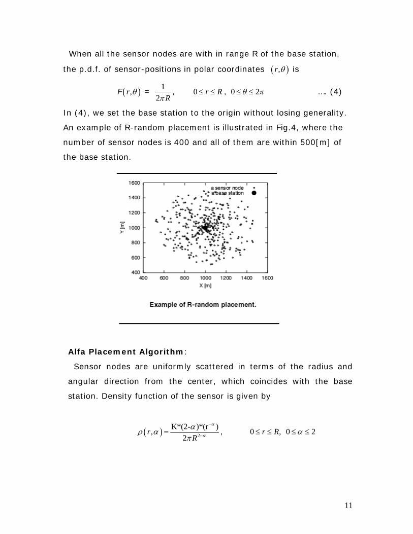
When all the sensor nodes are with in range R of the base station,

the p.d.f. of sensor-positions in polar coordinates ( ),r θ is

F ( ),r θ = 1

2 Rπ, 0 r R≤ ≤ , 0 2θ π≤ ≤ …. (4)

In (4), we set the base station to the origin without losing generality.

An example of R-random placement is illustrated in Fig.4, where the

number of sensor nodes is 400 and all of them are within 500[m] of

the base station.

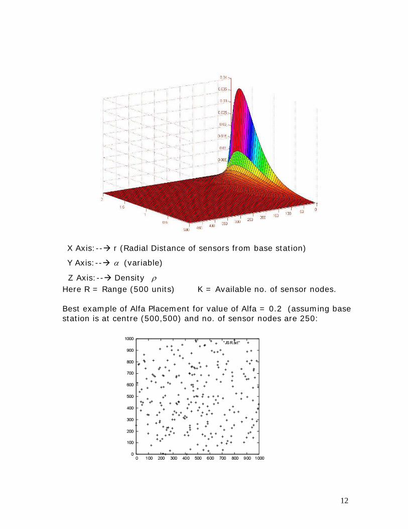
Alfa Placement Algorithm:

Sensor nodes are uniformly scattered in terms of the radius and

angular direction from the center, which coincides with the base

station. Density function of the sensor is given by

( ) 2

K*(2- )*(r ),2

rR

α

α

αρ απ

−

−= , 0 ,r R≤ ≤ 0 2α≤ ≤

12

X Axis:-- r (Radial Distance of sensors from base station)

Y Axis:-- α (variable)

Z Axis:-- Density ρ Here R = Range (500 units) K = Available no. of sensor nodes. Best example of Alfa Placement for value of Alfa = 0.2 (assuming base station is at centre (500,500) and no. of sensor nodes are 250:

13

Localization: In energy efficient routings, to rout a packet to the base station sometimes we do not need to know the exact positions of all the sensors. Only relative positions will do the work for us, that is, for each sensor, information about its neighbors and its distance from base station will suffice. For each sensor, exploring its neighbors and its distance from base station is a two step task:

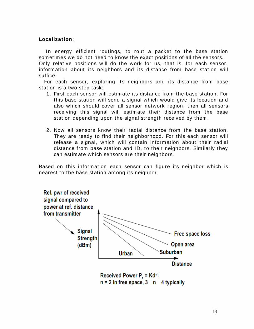
1. First each sensor will estimate its distance from the base station. For this base station will send a signal which would give its location and also which should cover all sensor network region, then all sensors receiving this signal will estimate their distance from the base station depending upon the signal strength received by them.

2. Now all sensors know their radial distance from the base station. They are ready to find their neighborhood. For this each sensor will release a signal, which will contain information about their radial distance from base station and ID, to their neighbors. Similarly they can estimate which sensors are their neighbors.

Based on this information each sensor can figure its neighbor which is nearest to the base station among its neighbor.

14

5. Routing Protocols: In the next few sub-sections, we will discuss the protocols tested in

detail. Briefly, the protocols are:

1. Direct communication, in which each node communicates directly

with the base station.

2. Diffusion-based algorithm utilizing only location data.

3. E3D: Diffusion based algorithm utilizing location, power levels, and

node load.

4. Random clustering, similar to LEACH, in which randomly chosen

group heads receive messages from all their members and forward

them to the base station.

5. An optimum clustering algorithm, in which clustering mechanisms

are applied after some iterations in order to obtain optimum cluster

formation based on physical location and power levels.

5.1 Direct Communication:

Each node is assumed to be within communication range of

the base station and that they are all aware who the base station is.

In the event that the nodes do not know who the base station is, the

base station could broadcast a message announcing itself as the base

station, after which all nodes in range will send to the specified base

station. So each node sends its data directly to the base station.

Eventually, each node will deplete its limited power supply and die.

When all nodes are dead and the system is said to be dead.

The main advantages of this algorithm lie in its simplicity.

There is no synchronization to be done between peer nodes, and

perhaps a simple broadcast message from the base station would

15

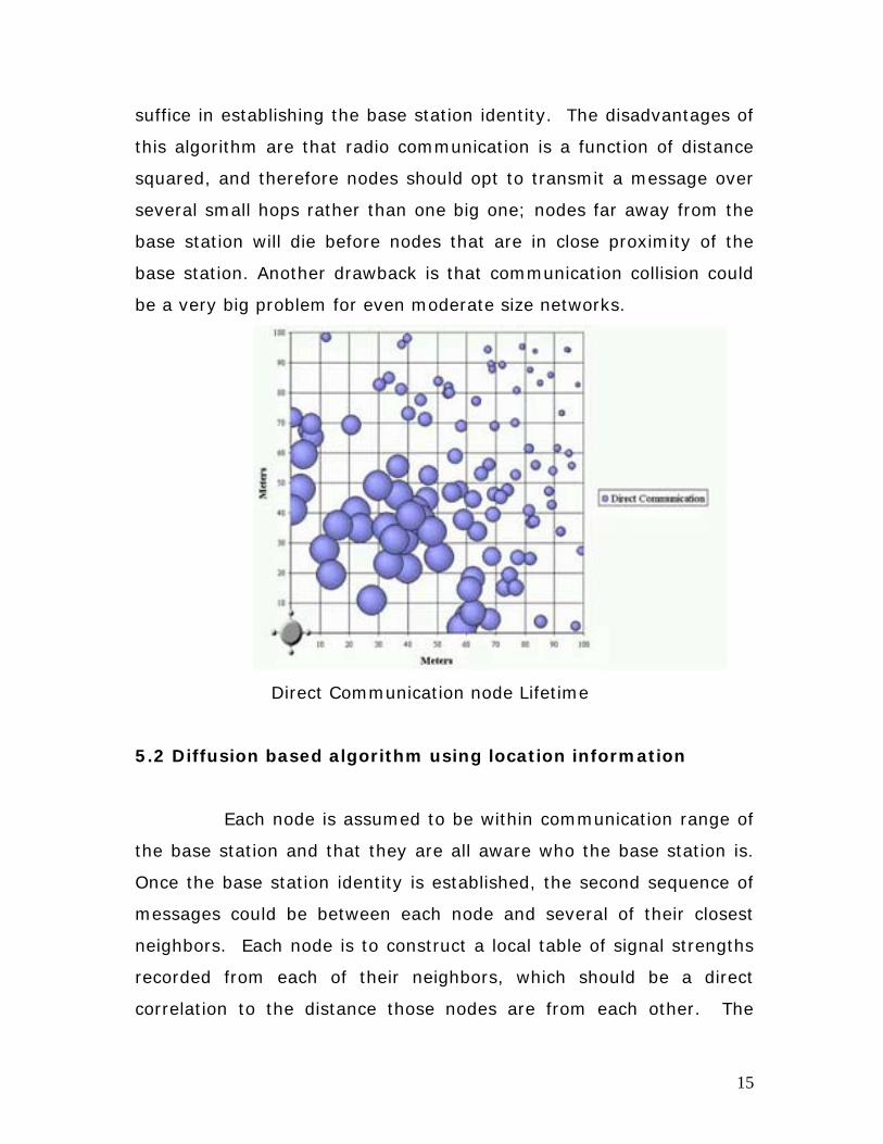
suffice in establishing the base station identity. The disadvantages of

this algorithm are that radio communication is a function of distance

squared, and therefore nodes should opt to transmit a message over

several small hops rather than one big one; nodes far away from the

base station will die before nodes that are in close proximity of the

base station. Another drawback is that communication collision could

be a very big problem for even moderate size networks.

Direct Communication node Lifetime

5.2 Diffusion based algorithm using location information

Each node is assumed to be within communication range of

the base station and that they are all aware who the base station is.

Once the base station identity is established, the second sequence of

messages could be between each node and several of their closest

neighbors. Each node is to construct a local table of signal strengths

recorded from each of their neighbors, which should be a direct

correlation to the distance those nodes are from each other. The

16

other value needed is the distance from each neighbor to the base

station, which can be figured out all within the same synchronization

messages. This setup phase needs only be completed once at the

startup of the system; therefore, it can be considered as constant cost

and should not affect the algorithm’s performance beyond the setup

phase.

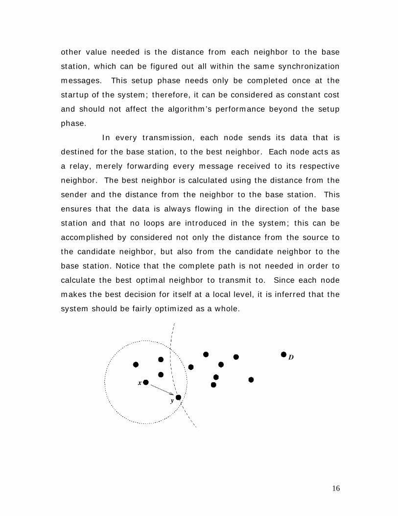
In every transmission, each node sends its data that is

destined for the base station, to the best neighbor. Each node acts as

a relay, merely forwarding every message received to its respective

neighbor. The best neighbor is calculated using the distance from the

sender and the distance from the neighbor to the base station. This

ensures that the data is always flowing in the direction of the base

station and that no loops are introduced in the system; this can be

accomplished by considered not only the distance from the source to

the candidate neighbor, but also from the candidate neighbor to the

base station. Notice that the complete path is not needed in order to

calculate the best optimal neighbor to transmit to. Since each node

makes the best decision for itself at a local level, it is inferred that the

system should be fairly optimized as a whole.

17

The main advantage of this system is its fairly light

complexity, which allows the synchronization of the neighboring nodes

to be done relatively inexpensive, and only once at the system

startup. The system also distributes the lifetime of the network a

little bit more efficiently.

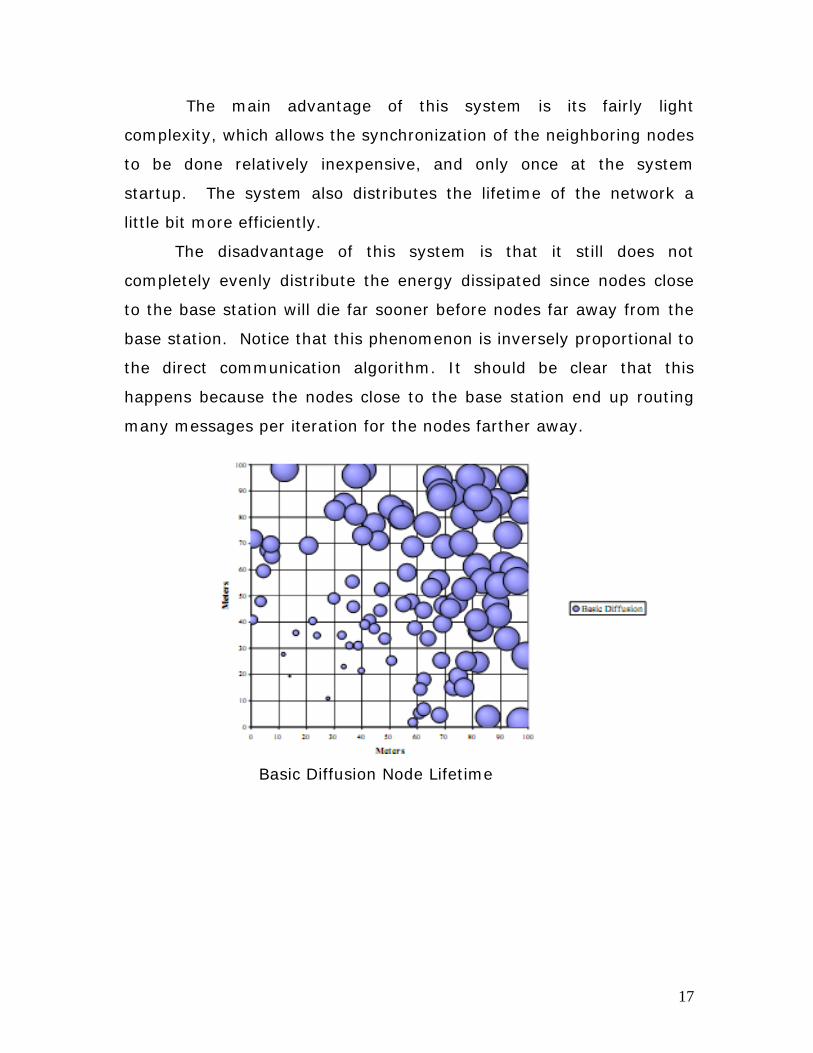
The disadvantage of this system is that it still does not

completely evenly distribute the energy dissipated since nodes close

to the base station will die far sooner before nodes far away from the

base station. Notice that this phenomenon is inversely proportional to

the direct communication algorithm. It should be clear that this

happens because the nodes close to the base station end up routing

many messages per iteration for the nodes farther away.

Basic Diffusion Node Lifetime

18

5.3 E3D: Energy-Efficient Distributed Dynamic Diffusion based

algorithm using location, power, and load as metrics

In addition to everything that the basic diffusion algorithm

performs, each node makes a list of suitable neighbors and ranks

them in order of preference, similar to the previous approach. Every

time that a node changes neighbors, the sender will require an

acknowledgement for its first message which will ensure that the

receiving node is still alive. If a time out occurs, the sending node will

choose another neighbor to transmit to and the whole process

repeats. Once communication is initiated, there will be no more

acknowledgements for any messages. Besides data messages, there

is an introduce exception messages which serve as explicit

synchronization messages. Only receivers can issue exception

messages, and are primarily used to tell the sending node to stop

sending and let the sender choose a different neighbor. An exception

message is generated in only three instances: the receiving node’s

queue is too large, the receiver’s power is less than the sender’s

power, and the receiver has passed a certain threshold which means

that it has very little power left.

At any time throughout the system’s lifetime, a receiver can

tell a sender not to transmit anymore because the receiver’s queues

are full. This should normally not happen, but in the event it does, an

exception message would alleviate the problem. In the current

schema, once the sending node receives an exception message and

removes his respective neighbor off his neighbor list, the sending

node will never consider that same neighbor again. We did this in

order to minimize the amount of control messages that would be

needed to be exchanged between peer nodes. However, future

19

considerations could be to place a receiving neighbor on probation in

the event of an exception message, and only permanently remove it

as a valid neighbor after a certain number of exception messages.

The second reason an exception message might be issued,

which is the more likely one, is when the receiver’s power is less than

the sender’s power, in which if the receiver’s power is less than the

specified threshold, it would then analyze the receiving packets for the

sender’s power levels. If the threshold was made too small, then by

the time the receiver managed to react and tell the sender to stop

sending, too much of its power supply had been depleted and its life

expectancy thereafter would be very limited while the sending node’s

life expectance would be much longer due to its less energy

consumption. Through empirical results, we concluded that the

optimum threshold is 50% of the receiver’s power levels when it in

order to equally distribute the power dissipation throughout the

network.

In order to avoid having to acknowledge every message or

even have heartbeat messages, we introduce an additional threshold

that will tell the receiving node when its battery supply is almost

gone. This threshold should be relatively small, in the 5~10% of total

power, and is used for telling the senders that their neighbors are

almost dead and that new more suitable neighbors should be elected.

The synchronization cost of e3D is two messages for each pair

of neighboring nodes. The rest of the decisions will be based on local

look-ups in its memory for the next best suitable neighbor to which it

should transmit to. Eventually, when all suitable neighbors are

exhausted, the nodes opt to transmit directly to the base station. By

looking at the empirical results obtained, it is only towards the end of

20

the system’s lifetime that the nodes decide to send directly to the

base station.

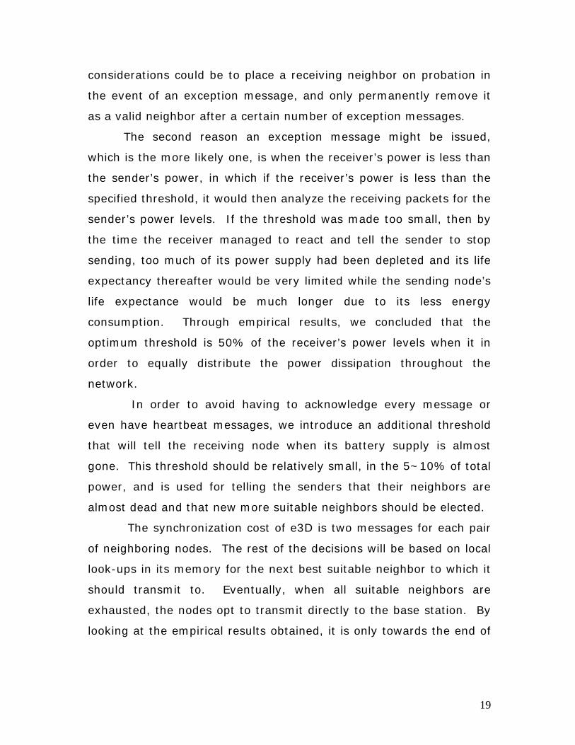
The main advantage of this algorithm is the near perfect system

lifetime where most nodes in the network live relatively the same

duration. The system distributes the lifetime and load on the network

better than the previous two approaches. The disadvantage when

compared to of this algorithm is its higher complexity, which requires

some synchronization messages throughout the lifetime of the

system. These synchronization message are very few, and therefore

worth the price in the event that the application calls for such strict

performance.

E3D Node Life Time

21

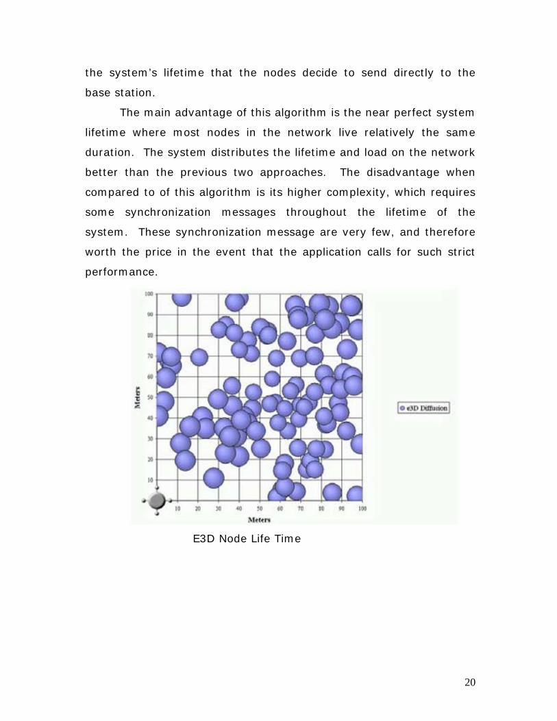
5.4 Random Clustering Based Algorithm

This algorithm is similar to LEACH, except there is no data

aggregation at the cluster heads. Random cluster heads are chosen

and clusters of nodes are established which will communicate with the

cluster heads.

The main advantage of this algorithm is the distribution of

power dissipation achieved by randomly choosing the group heads.

This yields a random distribution of node deaths. The disadvantage of

this algorithm is its relatively high complexity, which requires many

synchronization messages compared to e3D at regular intervals

throughout the lifetime of the system. Note that cluster heads should

not be chosen at every iteration since the cost of synchronization

would be very large in comparison to the number of messages that

would be actually transmitted. In our simulation, we used rounds of

20 iterations between choosing new cluster heads. The high cost of

22

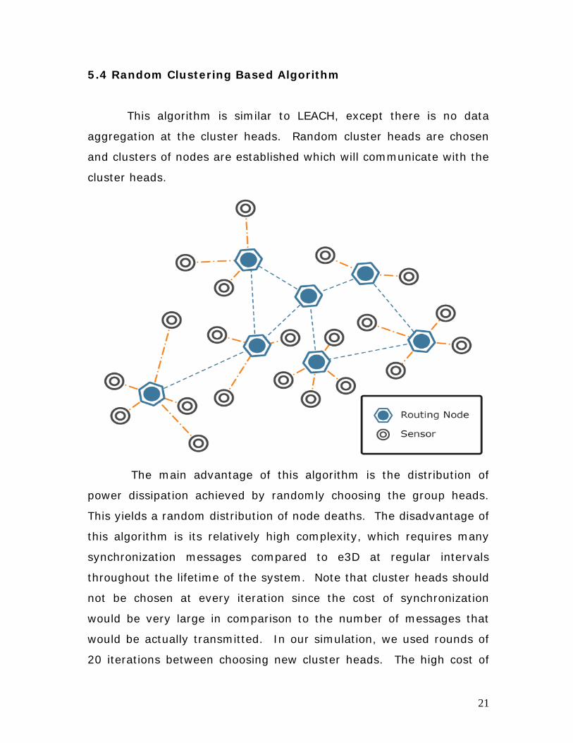
this schema is not justifiable for the performance gains over much

simpler schemes such as direct communication. As a whole, the

system does not live very long and has similar characteristics to direct

communication. Notice that the only difference in its perceived

performance from direct communication is that it randomly kills nodes

throughout the network rather than having all the nodes die on one

extreme of the network.

The nodes that are farther away would tend to die earlier

because the cluster heads that are farther away have much more

work to accomplish than cluster heads that are close to the base

station. The random clustering algorithm had a wide range of

performance results, which indicated that its performance was directly

related to the random cluster election; the worst case scenario had

worse performance by a factor of ten in terms of overall system

lifetime.

Clustering Node Lifetime

23

5.5 Ideal Clustering Based Algorithm

We implemented this algorithm for comparison purposes to

better evaluate the diffusion approach, especially that the random

clustering algorithm had a wide range of performance results since

everything depended on the random cluster election. The cost of

implementing this classical clustering algorithm in a real world

distributed system such as wireless sensor networks is energy

prohibitively high; however, it does offer us insight into the upper

bounds on the performance of clustering based algorithms.

We implemented k-Means clustering (k represents the number of

clusters) to form the clusters. The cluster heads are chosen to be the

clustroid nodes; the clustroid is the node in the cluster that minimizes

the sum of the cost metric to the other points of the corresponding

cluster. In electing the clustroid, the cost metric is calculated by

taking the distance squared between each corresponding node and

the candidate clustroid and divided by the candidate clustroid’s

respective power percentage levels. The metric was calculate after

some fixed iterations, and therefore yielded an optimal clustering

formation throughout the simulation. We experimented with the

number of clusters in order to find the optimum configuration, and

discovered that usually between 3 to 10 clusters is optimal for the 20

network topologies we utilized.

24

6. Sensor Network Simulator:

So for testing these various routing protocols, we designed a Sensor

Network Simulator.

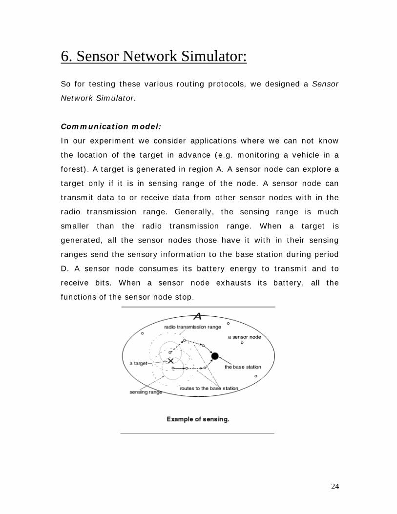
Communication model:

In our experiment we consider applications where we can not know

the location of the target in advance (e.g. monitoring a vehicle in a

forest). A target is generated in region A. A sensor node can explore a

target only if it is in sensing range of the node. A sensor node can

transmit data to or receive data from other sensor nodes with in the

radio transmission range. Generally, the sensing range is much

smaller than the radio transmission range. When a target is

generated, all the sensor nodes those have it with in their sensing

ranges send the sensory information to the base station during period

D. A sensor node consumes its battery energy to transmit and to

receive bits. When a sensor node exhausts its battery, all the

functions of the sensor node stop.

25

Parameters:

In this simulator, we can regulate certain parameters. The parameters

are the following:

• Buffer Limits: It is a realistic idea to set an upper limit to the

number of packets each sensor can receive and transmit in unit

time. In our experiments we have regulated the maximum

number of packets transmitted and received per simulation unit

time, as 200 and 400 respectively.

Max_trans_per_sim_cycle = 200

Max_recvd_per_sim_cycle = 200

• Activity Radii: The sensors are able to sense a target within a

given range of distance. Besides, for transmitting a given packet

transmitter range can be varied but energy consumed in it is

directly proportional to the square of distance transmitted. We

have regulated the sensing radius as:

Sense_radius = 60 units

• Energy Consumption Rates: Energy is spent in sensing and

broadcasting (we have assumed that the information regarding

the packets are broadcasted within the trans_radius) the

packets. We have assumed the following:

Sense_consumption = 1.9 µJ

Energy spent in transmission depends upon the signal

transmitted distance.

Energy_consumption = K d2

Where K = constant,

D = distance transmitted

26

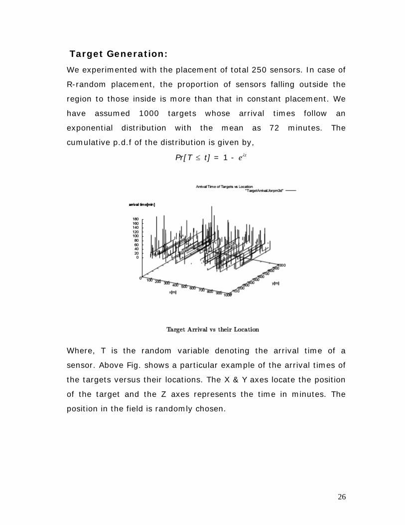
Target Generation:

We experimented with the placement of total 250 sensors. In case of

R-random placement, the proportion of sensors falling outside the

region to those inside is more than that in constant placement. We

have assumed 1000 targets whose arrival times follow an

exponential distribution with the mean as 72 minutes. The

cumulative p.d.f of the distribution is given by,

Pr[T ≤ t] = 1 - teλ

Where, T is the random variable denoting the arrival time of a

sensor. Above Fig. shows a particular example of the arrival times of

the targets versus their locations. The X & Y axes locate the position

of the target and the Z axes represents the time in minutes. The

position in the field is randomly chosen.

27

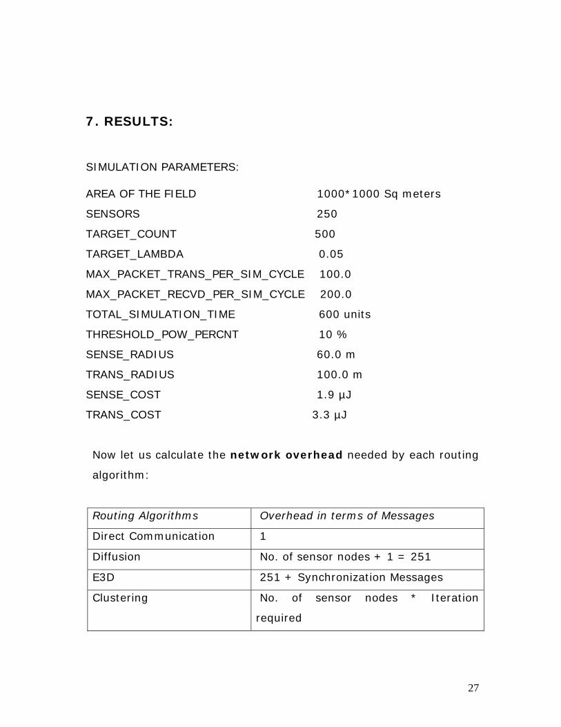
7. RESULTS:

SIMULATION PARAMETERS: AREA OF THE FIELD 1000*1000 Sq meters

SENSORS 250

TARGET_COUNT 500

TARGET_LAMBDA 0.05

MAX_PACKET_TRANS_PER_SIM_CYCLE 100.0

MAX_PACKET_RECVD_PER_SIM_CYCLE 200.0

TOTAL_SIMULATION_TIME 600 units

THRESHOLD_POW_PERCNT 10 %

SENSE_RADIUS 60.0 m

TRANS_RADIUS 100.0 m

SENSE_COST 1.9 µJ

TRANS_COST 3.3 µJ

Now let us calculate the network overhead needed by each routing

algorithm:

Routing Algorithms Overhead in terms of Messages

Direct Communication 1

Diffusion No. of sensor nodes + 1 = 251

E3D 251 + Synchronization Messages

Clustering No. of sensor nodes * Iteration

required

28

In direct Communication, since each sensor directly communicates

with the base station, there is no need of localization. Only base

station location information would be needed for sensors to get

started. That could be done by sending a signal from base station

from which all sensors will come to know about the base station

location.

In case of diffusion algorithm, neighbors are to be located. In order

to do that each sensor must once send a signal to its neighbors. In

our case we have 250 sensor nodes, so it need 251 messages to be

send here there to get the network working.

E3D need extra synchronization messages than diffusion algorithm,

in order to low the maintenance of network.

Network overhead for Cluster based approach is huge, since no. of

iterations required is always large in order to divide network into

clusters. In our experiment we implemented K-Mean clustering

algorithm to cluster the network.

K=20 i.e. network is to be divided into 20 clusters.

Average no. of iterations needed to divide the cluster is 9.

So network overhead = (No. of sensor nodes = 250)*(Iteration = 9)

= 2250

So from above results we can easily see that cluster based approach

is not enough energy efficient in a wireless sensor network deployed

in a remote energy constraint area.

So in next we will consider the other three efficient algorithms, and

will check which one is most efficient in different aspects.

29

Life of the WSN & Maintenance: We know a simple relation: For all D>=0, D2 >= D1

2 + D22 Where D = D1 + D2

Since energy consumed in transmitting a signal to distance is D is

proportional to the square of distance transmitted. We can easily

concede that for the same set of parameters and targets, network

equipped with Direct Communication protocol will run out of energy

faster than rest of the types of networks. Because for a long range

transmission sensor located far from base station will die very soon in

order to send signals to the base station. So this kind of network is

not efficient in a remote wide area.

Now let us compare the no. of sensors alive at time iterations for rest

of the routing algorithms for two different types of placements:

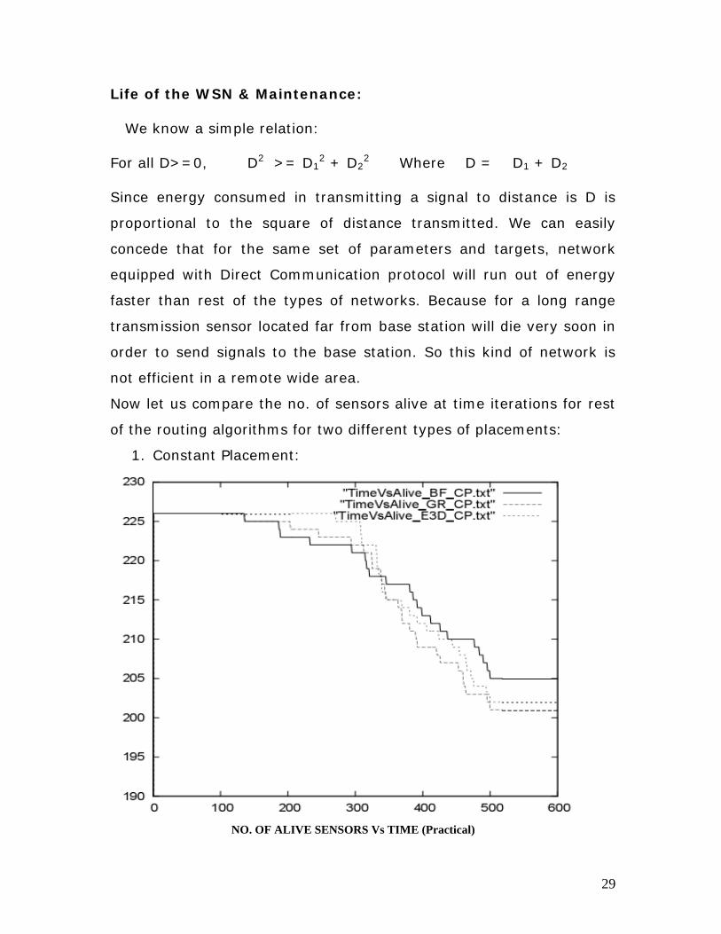
1. Constant Placement:

NO. OF ALIVE SENSORS Vs TIME (Practical)

30

We can see that almost all the sensors are alive for E3D algorithm for

quite long period of time, hence extending the network efficiency. For

other algorithms, as no. of dead sensors increase their efficiency will

decrease.

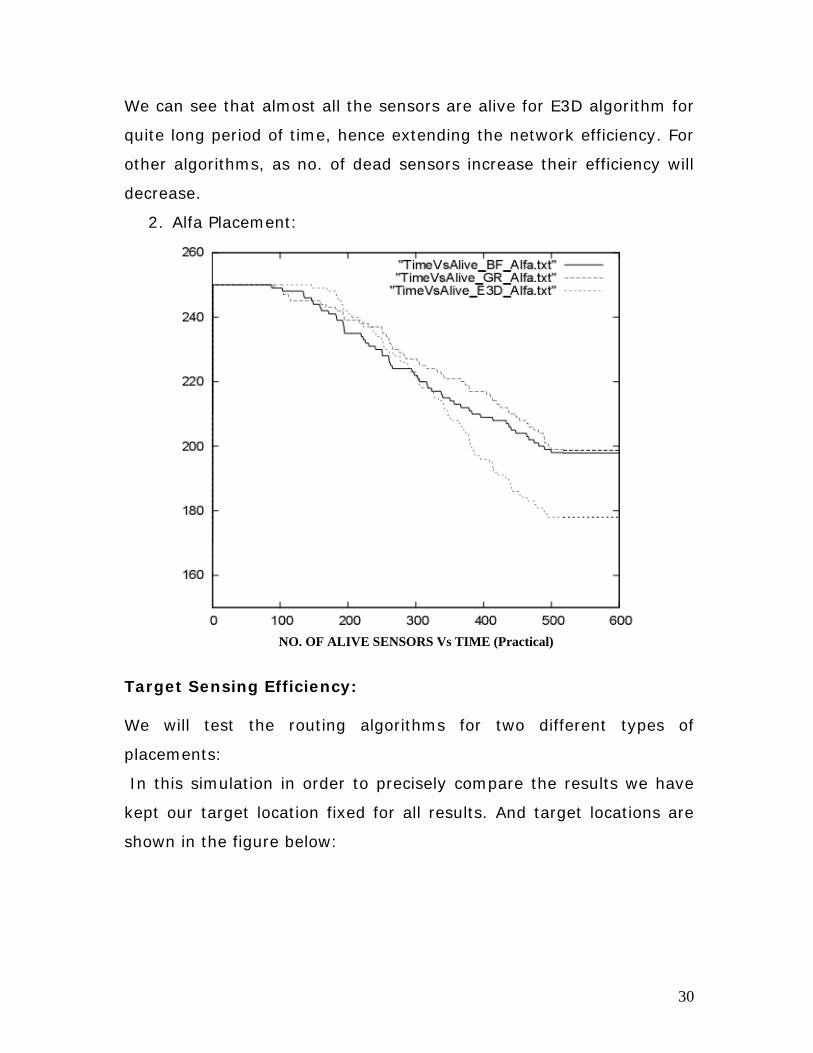
2. Alfa Placement:

NO. OF ALIVE SENSORS Vs TIME (Practical)

Target Sensing Efficiency: We will test the routing algorithms for two different types of

placements:

In this simulation in order to precisely compare the results we have

kept our target location fixed for all results. And target locations are

shown in the figure below:

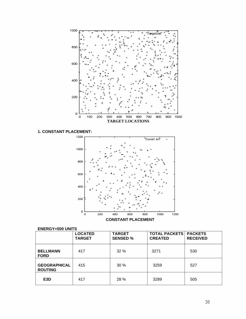
31

TARGET LOCATIONS 1. CONSTANT PLACEMENT:

CONSTANT PLACEMENT ENERGY=500 UNITS LOCATED

TARGET TARGET SENSED %

TOTAL PACKETS CREATED

PACKETS RECEIVED

BELLMANN FORD

417

32 %

3271

530

GEOGRAPHICAL ROUTING

415

30 %

3259

527

E3D

417

28 %

3289

505

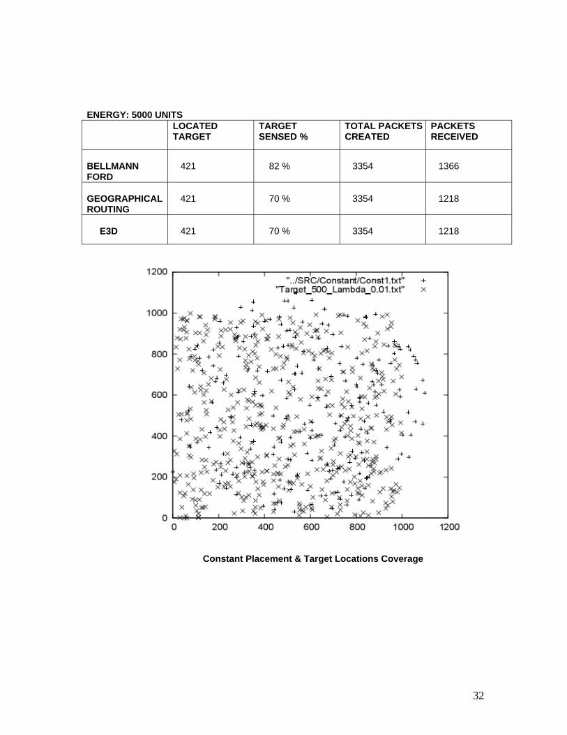
32

ENERGY: 5000 UNITS LOCATED

TARGET TARGET SENSED %

TOTAL PACKETS CREATED

PACKETS RECEIVED

BELLMANN FORD

421

82 %

3354

1366

GEOGRAPHICAL ROUTING

421

70 %

3354

1218

E3D

421

70 %

3354

1218

Constant Placement & Target Locations Coverage

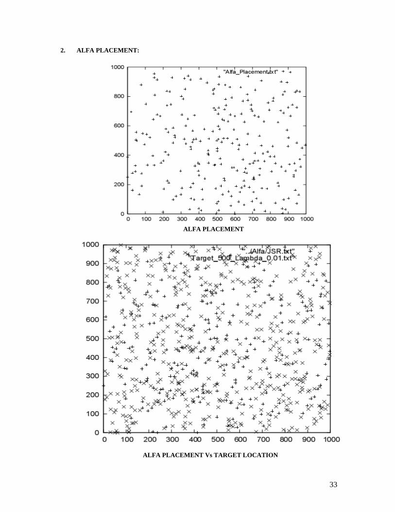
33

2. ALFA PLACEMENT:

ALFA PLACEMENT

ALFA PLACEMENT Vs TARGET LOCATION

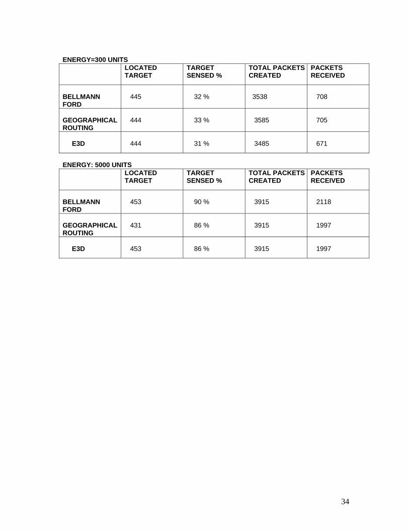
34

ENERGY=300 UNITS LOCATED

TARGET TARGET SENSED %

TOTAL PACKETS CREATED

PACKETS RECEIVED

BELLMANN FORD

445

32 %

3538

708

GEOGRAPHICAL ROUTING

444

33 %

3585

705

E3D

444

31 %

3485

671

ENERGY: 5000 UNITS LOCATED

TARGET TARGET SENSED %

TOTAL PACKETS CREATED

PACKETS RECEIVED

BELLMANN FORD

453

90 %

3915

2118

GEOGRAPHICAL ROUTING

431

86 %

3915

1997

E3D

453

86 %

3915

1997

35

Conclusion:

So from our simulation results we can observe that Diffusion

Based Algorithm (Geographical Routing) and E3D routing are energy

efficient algorithm which works fine for any placement strategies.

E3D routing is a little advancement of Geographical routing in order

to resolve maintenance problem for the network. But advantage gain

by E3D in maintenance end up with wasting lots of energy in

synchronizing the network which is redundant in remote area where

energy constraint is the biggest problem.

So we can deal with network life with its maintenance depending

upon the situations we have or the network we desire. Sometimes it

is not possible to achieve everything; we have to loose some in order

to gain some.

36

REFERENCES:

[1]: Using Geospatial Information in Sensor Networks by John Heidemann and

Nirupama Bulusu

[2]: Performance study of node placement in sensor networks by Mika ISHIZUKA

and Masaki AIDA

[3]: Distributed localization in wireless sensor networks: a quantative comparison by

Koen Langendoen and Niels Reijers

[4]: A Directionality based location discovery scheme for Wireless Sensor Networks

by Asis Nasipuri and Kai Li

[5]: Localization in sensor networks by Andreas Savvides and Mani Srivastava.

[6]: An Energy-Efficient Routing Algorithm for Wireless Sensor Networks by - Ioan

Raicu, Loren Schwiebert, Scott Fowler, Sandeep K.S. Gupta

[7]: Relative density based K- Nearest neighbors clustering algorithm: QING-BA0

LIU, SU DENG, CHANG-HUI LU, BO WANG, YONG-FENG ZHOU

[8]: Energy Efficient Cluster Formation in Wireless Sensor Networks

By Malka N. Halgamuge, *Siddeswara Mayura Guru and Andrew Jennings

[9]: An efficient K-Mean clustering algorithm: Analysis and Implementation by

Tapas Kunungo, David M. Mount

[10]: Energy-Efficient Routing Algorithms in Wireless Sensor Networks: e3D

Diffusion vs. Clustering, by Ioan Raicu

[11] K. M. Sivalingam, M.B. and P. Agrawal, “Low Power Link and Access

Protocols for Wireless Multimedia Networks”, IEEE VTC’97, May 1997.

[12] M. Stemm, P. Gauther, D. Harada and R. Katz, “Reducing Power Consumption of

Network Interfaces in Hand-Held Devices”, 3rd Intl. Workshop on Mobile Multimedia

Communications, Sept. 1996.

[13] D Estrin, R Govindan, J Heidemann, S Kumar, “Next Century Challenges:

Scalable Coordination in Sensor Networks”, Proceedings of Mobicom 1999.

[14] R Ramanathan, R Hain, “Topology Control of Multihop Wireless Networks

Using Transmit Power Adjustment”, Proceeding Infocom 2000.

[15] J Hill, R Szewczyk, A Woo, S Hollar, D Culler, K Pister, “System architecture

directions for network sensors”, ASPLOS 2000.

37

[16] W. Heinzelman, A. Chandrakasan, and H. Balakrishnan, “Energy-Efficient

Communication Protocol for Wireless Microsensor Networks”, Hawaiian Int'l Conf. on

Systems Science, January 2000.

[17] S. Lindsey and C. Raghavendra, “PEGASIS: Power-Efficient GAthering in

Sensor Information Systems”, International Conference on Communications, 2001.