Embed Size (px)
Citation preview

ENERGY-EFFICIENT MANAGEMENT OF
HETEROGENEOUS
WIRELESS SENSOR NETWORKS
Inauguraldissertationder Philosophisch-naturwissenschaftlichen Fakultat
der Universitat Bern
vorgelegt von
Gerald Wagenknecht
von Gorlitz, Deutschland
Leiter der Arbeit:Professor Dr. Torsten Braun
Institut fur Informatik und angewandte Mathematik
Von der Philosophisch-naturwissenschaftlichen Fakultat angenommen.
Der Dekan:Bern, 06.05.2013 Prof. Dr. Silvio Decurtins


Abstract
Various applications for the purposes of event detection, localization, and mon-itoring can benefit from the use of wireless sensor networks (WSNs). Wirelesssensor networks are generally easy to deploy, with flexible topology and can sup-port diversity of tasks thanks to the large variety of sensors that can be attached tothe wireless sensor nodes. To guarantee the efficient operation of such a heteroge-neous wireless sensor networks during its lifetime an appropriate management isnecessary.
Typically, there are three management tasks, namely monitoring, (re) config-uration, and code updating. On the one hand, status information, such as bat-tery state and node connectivity, of both the wireless sensor network and the sen-sor nodes has to be monitored. And on the other hand, sensor nodes have to be(re)configured, e.g., setting the sensing interval. Most importantly, new applica-tions have to be deployed as well as bug fixes have to be applied during the net-work lifetime. All management tasks have to be performed in a reliable, time- andenergy-efficient manner.
The ability to disseminate data from one sender to multiple receivers in a re-liable, time- and energy-efficient manner is critical for the execution of the man-agement tasks, especially for code updating. Using multicast communication inwireless sensor networks is an efficient way to handle such traffic pattern. Due tothe nature of code updates a multicast protocol has to support bulky traffic and end-to-end reliability. Further, the limited resources of wireless sensor nodes demandan energy-efficient operation of the multicast protocol. Current data disseminationschemes do not fulfil all of the above requirements.
In order to close the gap, we designed the Sensor Node Overlay Multicast(SNOMC) protocol such that to support a reliable, time-efficient and energy-efficientdissemination of data from one sender node to multiple receivers. In contrast toother multicast transport protocols, which do not support reliability mechanisms,SNOMC supports end-to-end reliability using a NACK-based reliability mecha-nism. The mechanism is simple and easy to implement and can significantly reducethe number of transmissions. It is complemented by a data acknowledgement aftersuccessful reception of all data fragments by the receiver nodes. In SNOMC threedifferent caching strategies are integrated for an efficient handling of necessary re-transmissions, namely, caching on each intermediate node, caching on branchingnodes, or caching only on the sender node. Moreover, an option was included topro-actively request missing fragments.
SNOMC was evaluated both in the OMNeT++ simulator and in our in-housereal-world testbed and compared to a number of common data dissemination pro-tocols, such as Flooding, MPR, TinyCubus, PSFQ, and both UDP and TCP. Theresults showed that SNOMC outperforms the selected protocols in terms of trans-mission time, number of transmitted packets, and energy-consumption. Moreover,

we showed that SNOMC performs well with different underlying MAC protocols,which support different levels of reliability and energy-efficiency. Thus, SNOMCcan offer a robust, high-performing solution for the efficient distribution of codeupdates and management information in a wireless sensor network.
To address the three management tasks, in this thesis we developed the Man-agement Architecture for Wireless Sensor Networks (MARWIS). MARWIS is specif-ically designed for the management of heterogeneous wireless sensor networks. Adistinguished feature of its design is the use of wireless mesh nodes as backbone,which enables diverse communication platforms and offloading functionality fromthe sensor nodes to the mesh nodes. This hierarchical architecture allows for ef-ficient operation of the management tasks, due to the organisation of the sensornodes into small sub-networks each managed by a mesh node. Furthermore, we de-veloped a intuitive -based graphical user interface, which allows non-expert usersto easily perform management tasks in the network. In contrast to other manage-ment frameworks, such as Mate, MANNA, TinyCubus, or code dissemination pro-tocols, such as Impala, Trickle, and Deluge, MARWIS offers an integrated solutionmonitoring, configuration and code updating of sensor nodes.
Integration of SNOMC into MARWIS further increases performance efficiencyof the management tasks. To our knowledge, our approach is the first one, whichoffers a combination of a management architecture with an efficient overlay mul-ticast transport protocol. This combination of SNOMC and MARWIS supportsreliably, time- and energy-efficient operation of a heterogeneous wireless sensornetwork.
b


Contents
Contents i
List of Figures v
List of Tables viii
1 Introduction 11.1 Overview . . . . . . . . . . . . . . . . . . . . . . . . . . . . . . 11.2 Problem Statement . . . . . . . . . . . . . . . . . . . . . . . . . 31.3 Contributions . . . . . . . . . . . . . . . . . . . . . . . . . . . . 41.4 Thesis Outline . . . . . . . . . . . . . . . . . . . . . . . . . . . . 6
2 Related Work 92.1 Hardware Platforms . . . . . . . . . . . . . . . . . . . . . . . . . 9
2.1.1 PC Engines ALIX . . . . . . . . . . . . . . . . . . . . . 102.1.2 Crossbow Tmote Sky / TelosB . . . . . . . . . . . . . . . 112.1.3 Scatterweb Modular Sensor Board . . . . . . . . . . . . . 122.1.4 Crossbow MICAz . . . . . . . . . . . . . . . . . . . . . 132.1.5 BTnode . . . . . . . . . . . . . . . . . . . . . . . . . . . 14
2.2 Operating Systems . . . . . . . . . . . . . . . . . . . . . . . . . 152.2.1 ADAM . . . . . . . . . . . . . . . . . . . . . . . . . . . 152.2.2 Contiki Operating System . . . . . . . . . . . . . . . . . 17
2.3 Evaluation Platforms . . . . . . . . . . . . . . . . . . . . . . . . 192.3.1 OMNeT++ Network Simulation Framework . . . . . . . . 202.3.2 Wisebed WSN Testbed Controlled by TARWIS . . . . . . 212.3.3 Energy Measurement . . . . . . . . . . . . . . . . . . . . 22
2.4 Multicast in Wireless Sensor Networks . . . . . . . . . . . . . . . 232.4.1 Multicast Routing . . . . . . . . . . . . . . . . . . . . . 232.4.2 Multicast Transport . . . . . . . . . . . . . . . . . . . . . 28
2.5 Data Dissemination Protocols . . . . . . . . . . . . . . . . . . . . 332.5.1 Directed Diffusion . . . . . . . . . . . . . . . . . . . . . 332.5.2 Pump Slowly, Fetch Quickly (PSFQ) . . . . . . . . . . . 372.5.3 Flooding . . . . . . . . . . . . . . . . . . . . . . . . . . 382.5.4 MPR . . . . . . . . . . . . . . . . . . . . . . . . . . . . 39
i

2.6 Contiki Protocol Stack . . . . . . . . . . . . . . . . . . . . . . . 412.6.1 Link Layer Protocols . . . . . . . . . . . . . . . . . . . . 422.6.2 Network Layer Protocols . . . . . . . . . . . . . . . . . . 45
2.7 Management of Wireless Sensor Networks . . . . . . . . . . . . . 492.7.1 Management Frameworks . . . . . . . . . . . . . . . . . 492.7.2 Code Dissemination Protocols . . . . . . . . . . . . . . . 51
2.8 Conclusions . . . . . . . . . . . . . . . . . . . . . . . . . . . . . 52
I SNOMC: A Overlay Multicast Transport Protocol for WirelessSensor Networks 54
3 Protocol Design and Architecture 553.1 Introduction . . . . . . . . . . . . . . . . . . . . . . . . . . . . . 553.2 Protocol Design on Application Layer . . . . . . . . . . . . . . . 563.3 Protocol Description . . . . . . . . . . . . . . . . . . . . . . . . 57
3.3.1 Joining Phase . . . . . . . . . . . . . . . . . . . . . . . . 583.3.2 Data Transmission Phase and Caching . . . . . . . . . . . 623.3.3 End-to-End Reliability . . . . . . . . . . . . . . . . . . . 64
3.4 Conclusions . . . . . . . . . . . . . . . . . . . . . . . . . . . . . 67
4 SNOMC Implementation 694.1 Introduction . . . . . . . . . . . . . . . . . . . . . . . . . . . . . 694.2 SNOMC Implementation in OMNeT++ . . . . . . . . . . . . . . 69
4.2.1 Protocol Stack . . . . . . . . . . . . . . . . . . . . . . . 694.2.2 Protocol Operation . . . . . . . . . . . . . . . . . . . . . 714.2.3 CC2420 Radio . . . . . . . . . . . . . . . . . . . . . . . 734.2.4 Data Structures and Messages . . . . . . . . . . . . . . . 75
4.3 SNOMC Implementation in Contiki OS . . . . . . . . . . . . . . 764.3.1 Joining Procedure . . . . . . . . . . . . . . . . . . . . . . 764.3.2 Data Transmission Procedure . . . . . . . . . . . . . . . 794.3.3 Fragmentation, Caching, and Buffer . . . . . . . . . . . . 824.3.4 SNOMC Control/Sender Process and Packet Queues . . . 83
4.4 Conclusions . . . . . . . . . . . . . . . . . . . . . . . . . . . . . 85
5 SNOMC Evaluation 875.1 Introduction . . . . . . . . . . . . . . . . . . . . . . . . . . . . . 875.2 SNOMC Evaluation of Simulation Results . . . . . . . . . . . . . 88
5.2.1 Protocol Stack . . . . . . . . . . . . . . . . . . . . . . . 885.2.2 Simulation Scenarios . . . . . . . . . . . . . . . . . . . . 895.2.3 Transmission Times . . . . . . . . . . . . . . . . . . . . 915.2.4 Number of Transmissions . . . . . . . . . . . . . . . . . 925.2.5 Energy Consumption . . . . . . . . . . . . . . . . . . . . 93
5.3 SNOMC Evaluation in Real-World Testbed . . . . . . . . . . . . 94
ii

5.3.1 Protocol Stack . . . . . . . . . . . . . . . . . . . . . . . 945.3.2 Experimentation Scenarios . . . . . . . . . . . . . . . . . 955.3.3 Transmission Times . . . . . . . . . . . . . . . . . . . . 965.3.4 Number of Transmissions . . . . . . . . . . . . . . . . . 1015.3.5 Energy Consumption . . . . . . . . . . . . . . . . . . . . 103
5.4 Comparison of Simulated and Real-World Results . . . . . . . . . 1065.5 Conclusions . . . . . . . . . . . . . . . . . . . . . . . . . . . . . 107
II MARWIS: A Management Architecture for Wireless Sensor Net-works 109
6 Management Architecture and Protocol Design 1116.1 Introduction . . . . . . . . . . . . . . . . . . . . . . . . . . . . . 1116.2 Management Scenario and Tasks . . . . . . . . . . . . . . . . . . 1126.3 Management Architecture . . . . . . . . . . . . . . . . . . . . . 114
6.3.1 Management Station with Management System for Wire-less Mesh Networks . . . . . . . . . . . . . . . . . . . . 114
6.3.2 Mesh Node with MARWIS Server . . . . . . . . . . . . . 1156.3.3 Sensor Node with SN Agent . . . . . . . . . . . . . . . . 116
6.4 WSN Management Protocols . . . . . . . . . . . . . . . . . . . . 1166.4.1 WSN Monitoring Protocol . . . . . . . . . . . . . . . . . 1166.4.2 WSN Configuration Protocol . . . . . . . . . . . . . . . . 1196.4.3 WSN Code Update Protocol . . . . . . . . . . . . . . . . 120
6.5 Conclusions . . . . . . . . . . . . . . . . . . . . . . . . . . . . . 123
7 Implementation of MARWIS and Demonstrator 1257.1 Introduction . . . . . . . . . . . . . . . . . . . . . . . . . . . . . 1257.2 MARWIS Server Implementation . . . . . . . . . . . . . . . . . 125
7.2.1 Management Modules . . . . . . . . . . . . . . . . . . . 1267.2.2 Database Implementation . . . . . . . . . . . . . . . . . . 129
7.3 Management Station with Graphical User Interface . . . . . . . . 1347.4 Sensor Node Agent Implementation . . . . . . . . . . . . . . . . 136
7.4.1 Addressing . . . . . . . . . . . . . . . . . . . . . . . . . 1367.4.2 Sensor Node Monitor . . . . . . . . . . . . . . . . . . . . 1377.4.3 Sensor Node Configurator . . . . . . . . . . . . . . . . . 1387.4.4 Code Updater . . . . . . . . . . . . . . . . . . . . . . . . 138
7.5 MARWIS Demonstrator . . . . . . . . . . . . . . . . . . . . . . 1397.6 Conclusions . . . . . . . . . . . . . . . . . . . . . . . . . . . . . 140
8 SNOMC Integration into MARWIS 1418.1 Introduction . . . . . . . . . . . . . . . . . . . . . . . . . . . . . 1418.2 Architecture . . . . . . . . . . . . . . . . . . . . . . . . . . . . . 1428.3 Implementation . . . . . . . . . . . . . . . . . . . . . . . . . . . 145
iii

8.3.1 Implementation of SNOMC on Wireless Mesh Nodes . . . 1458.3.2 Adaptation of the MARWIS Graphical User Interface . . . 146
8.4 Evaluation . . . . . . . . . . . . . . . . . . . . . . . . . . . . . . 1468.4.1 Evaluation Scenario . . . . . . . . . . . . . . . . . . . . 1468.4.2 Time-Efficient Communication . . . . . . . . . . . . . . 1488.4.3 Energy-Efficient Operation . . . . . . . . . . . . . . . . . 150
8.5 Conclusions . . . . . . . . . . . . . . . . . . . . . . . . . . . . . 152
9 Conclusions and Outlook 1539.1 Addressed Challenges . . . . . . . . . . . . . . . . . . . . . . . . 1539.2 Main Contributions and Summary . . . . . . . . . . . . . . . . . 1549.3 Outlook . . . . . . . . . . . . . . . . . . . . . . . . . . . . . . . 156
Bibliography 159
List of Publications 173
Curriculum Vitae 176
iv

List of Figures
1.1 Applications utilizing wireless sensor networks. . . . . . . . . . . 2
2.1 PC Engines ALIX 3d2 Board[81] . . . . . . . . . . . . . . . . . . 102.2 Crossbow Tmote Sky. . . . . . . . . . . . . . . . . . . . . . . . . 112.3 Scatterweb MSB430. . . . . . . . . . . . . . . . . . . . . . . . . 122.4 Crossbow MICAz[28] . . . . . . . . . . . . . . . . . . . . . . . . 132.5 BTnode platform. . . . . . . . . . . . . . . . . . . . . . . . . . . 142.6 Steps of the build and setup process for a node [113] . . . . . . . 162.7 Partitioning in Contiki: the core and loadable programs in RAM
and ROM. [38] . . . . . . . . . . . . . . . . . . . . . . . . . . . 172.8 Wisebed testbed at University of Bern. . . . . . . . . . . . . . . . 212.9 Directed Diffusion: interest propagation. . . . . . . . . . . . . . . 342.10 Directed Diffusion: gradient establishment. . . . . . . . . . . . . 352.11 Directed Diffusion: reinforcement. . . . . . . . . . . . . . . . . . 352.12 Directed Diffusion: multiple sinks. . . . . . . . . . . . . . . . . . 362.13 Directed Diffusion: local repair. . . . . . . . . . . . . . . . . . . 362.14 PSFQ: pump operation. . . . . . . . . . . . . . . . . . . . . . . . 372.15 PSFQ: fetch operation. . . . . . . . . . . . . . . . . . . . . . . . 382.16 PSFQ: pro-active fetch operation. . . . . . . . . . . . . . . . . . 382.17 Flooding. . . . . . . . . . . . . . . . . . . . . . . . . . . . . . . 392.18 Multipoint Relay. . . . . . . . . . . . . . . . . . . . . . . . . . . 402.19 TinyCubus. . . . . . . . . . . . . . . . . . . . . . . . . . . . . . 412.20 MAC and RDC protocols of NullMAC, ContikiMAC and BEAM. 422.21 ContikiMAC: unicast transmission[33]. . . . . . . . . . . . . . . 432.22 ContikiMAC: broadcast transmission[33]. . . . . . . . . . . . . . 442.23 BEAM: using short beacon strobes [13]. . . . . . . . . . . . . . . 442.24 BEAM: using beacon strobes including payload [13]. . . . . . . . 452.25 The protocol stack in Contiki. . . . . . . . . . . . . . . . . . . . 462.26 TCP and µIP header. . . . . . . . . . . . . . . . . . . . . . . . . 462.27 UDP and µIP header. . . . . . . . . . . . . . . . . . . . . . . . . 47
3.1 SNOMC: possible scenario. . . . . . . . . . . . . . . . . . . . . . 573.2 SNOMC: Joining phase, sender driven mode. . . . . . . . . . . . 583.3 SNOMC: messages for sender-driven joining. . . . . . . . . . . . 60
v

3.4 SNOMC: Joining phase, receiver driven mode. . . . . . . . . . . 613.5 SNOMC: messages for receiver-driven joining. . . . . . . . . . . 613.6 SNOMC: Transmission phase, no caching. . . . . . . . . . . . . . 623.7 SNOMC: Transmission phase, caching on branching nodes. . . . . 633.8 SNOMC: Transmission phase, caching on forwarding nodes. . . . 633.9 SNOMC: Transmission phase, using broadcast transmissions. . . . 643.10 SNOMC: data message. . . . . . . . . . . . . . . . . . . . . . . . 643.11 SNOMC: Reliability, caching only on sender node. . . . . . . . . 653.12 SNOMC: Reliability, caching on branching node. . . . . . . . . . 663.13 SNOMC: Reliability, caching on each intermediate node, pro-active. 663.14 SNOMC: reliability messages. . . . . . . . . . . . . . . . . . . . 67
4.1 OMNeT++: protocol stack. . . . . . . . . . . . . . . . . . . . . . 704.2 OMNeT++: SNOMC state machine, sender node. . . . . . . . . . 724.3 OMNeT++: SNOMC state machine, receiver nodes. . . . . . . . . 724.4 OMNeT++: SNOMC state machine, forwarding/branching nodes. 734.5 OMNeT++: CC2420 state machine. . . . . . . . . . . . . . . . . 744.6 SNOMC: data structures. . . . . . . . . . . . . . . . . . . . . . . 754.7 SNOMC control process: joining procedure, sender node. . . . . . 774.8 SNOMC control process: joining procedure, other nodes. . . . . . 784.9 SNOMC control process: data transmission, sender node. . . . . . 794.10 SNOMC control process: data transmission, receiver nodes. . . . 804.11 SNOMC control process: data transmission, other nodes. . . . . . 814.12 Buffer structure. . . . . . . . . . . . . . . . . . . . . . . . . . . . 834.13 SNOMC sender process: sending messages . . . . . . . . . . . . 844.14 SNOMC control process: receiving messages . . . . . . . . . . . 85
5.1 Simulation protocol stack. . . . . . . . . . . . . . . . . . . . . . 885.2 Simulation scenarios. . . . . . . . . . . . . . . . . . . . . . . . . 895.3 Evaluation: transmission time. . . . . . . . . . . . . . . . . . . . 915.4 Evaluation: number of transmitted packets. . . . . . . . . . . . . 935.5 Evaluation: energy consumption per node and per transmitted byte. 945.6 Real-World protocol stack. . . . . . . . . . . . . . . . . . . . . . 955.7 Evaluation scenario 1. . . . . . . . . . . . . . . . . . . . . . . . . 965.8 Evaluation scenario 2. . . . . . . . . . . . . . . . . . . . . . . . . 975.9 Evaluation scenario 3. . . . . . . . . . . . . . . . . . . . . . . . . 985.10 Evaluation: transmission time, scenario 1. . . . . . . . . . . . . . 995.11 Evaluation: transmission time, scenario 2. . . . . . . . . . . . . . 1005.12 Evaluation: transmission time, scenario 3. . . . . . . . . . . . . . 1015.13 Evaluation: number of transmitted packets, scenario 1. . . . . . . 1025.14 Evaluation: number of transmitted packets, scenario 2. . . . . . . 1035.15 Evaluation: energy consumption, scenario 1. . . . . . . . . . . . . 1045.16 Evaluation: energy consumption, scenario 2. . . . . . . . . . . . . 105
vi

6.1 A possible scenario for heterogeneous wireless sensor networkswith management devices. . . . . . . . . . . . . . . . . . . . . . 113
6.2 Architecture of the MARWIS components. . . . . . . . . . . . . . 1156.3 WSN monitor queries the mesh nodes . . . . . . . . . . . . . . . 1176.4 User requests sensor node information directly. . . . . . . . . . . 1176.5 Management station requests database information from the mesh
nodes. . . . . . . . . . . . . . . . . . . . . . . . . . . . . . . . . 1186.6 The WSN configuring protocol. . . . . . . . . . . . . . . . . . . 1196.7 A new sensor node joins the sensor sub-network. . . . . . . . . . 1206.8 The image gets uploaded to all affected mesh nodes. . . . . . . . . 1216.9 The user asks for all available images. . . . . . . . . . . . . . . . 1216.10 The user initiates the code update for the sensor node. . . . . . . . 122
7.1 MARWIS server messages for retirieving information from thesensor nodes. . . . . . . . . . . . . . . . . . . . . . . . . . . . . 127
7.2 MARWIS server messages for configuration and code update. . . 1287.3 User interface: network overview . . . . . . . . . . . . . . . . . . 1357.4 User interface: sensor node overview. . . . . . . . . . . . . . . . 1357.5 SN Agent: addressing. . . . . . . . . . . . . . . . . . . . . . . . 1377.6 A possible scenario for heterogeneous WSNs with management
devices. . . . . . . . . . . . . . . . . . . . . . . . . . . . . . . . 139
8.1 SNOMC in a heterogeneous MARWIS scenario. . . . . . . . . . . 1428.2 SNOMC integrated into the MARWIS architecture. . . . . . . . . 1428.3 Protocol stack containing SNOMC in the heterogeneous MARWIS
architecture. . . . . . . . . . . . . . . . . . . . . . . . . . . . . . 1438.4 Addressing scheme of the nodes in the MARWIS architecture. . . 1448.5 SNOMC: structures. . . . . . . . . . . . . . . . . . . . . . . . . 1458.6 Evaluation scenario using Wisebed testbed. . . . . . . . . . . . . 1478.7 Evaluation of reliable and time-efficient communication. . . . . . 1488.8 Evaluation: transmission time, code update (1392 bytes). . . . . . 1498.9 Evaluation: transmission time, configuration command (20 bytes). 1508.10 Evaluation: energy consumption, code update (1392 bytes). . . . . 1518.11 Evaluation: energy consumption, configuration command (20 bytes).151
vii

List of Tables
2.1 Overview over multicast routing protocols. . . . . . . . . . . . . . 242.2 Overview over multicast transport protocols. . . . . . . . . . . . . 292.3 Overview over management frameworks. . . . . . . . . . . . . . 492.4 Overview over code dissemination protocols. . . . . . . . . . . . 51
5.1 MAC Protocol Parameters. . . . . . . . . . . . . . . . . . . . . . 895.2 Simulation Parameters. . . . . . . . . . . . . . . . . . . . . . . . 905.3 Energy Consumption of the CC2420 Radio Transceiver. . . . . . . 90
7.1 Database table sensornodes for the sensor nodes. . . . . . . . 1297.2 Database table meshnodes for the mesh nodes. . . . . . . . . . 1297.3 Database table wmn for the mesh network. . . . . . . . . . . . . . 1297.4 Database table wsn for the sensor network. . . . . . . . . . . . . 1307.5 Database table sn properties storing the values of the sensor
node properties. . . . . . . . . . . . . . . . . . . . . . . . . . . . 1307.6 Database table properties storing descriptive information about
the properties. . . . . . . . . . . . . . . . . . . . . . . . . . . . . 1307.7 Database table sensor state storing the state of the sensors. . 1307.8 Database table sn platforms for the sensor node platforms. . . 1317.9 Database table mn platform for the mesh node platforms. . . . 1317.10 Database table os platform for the operating system platforms. 1317.11 Database table pics storing the pictures used by the GUI. . . . . 1317.12 Database table sn images storing which images running on which
sensor nodes. . . . . . . . . . . . . . . . . . . . . . . . . . . . . 1327.13 Database table images storing the images. . . . . . . . . . . . . 1327.14 Database table sn values storing the measured sensor values. . 133
8.1 Possible protocol combinations. . . . . . . . . . . . . . . . . . . 146
viii

Chapter 1
Introduction
Wireless sensor networks are widely used by real-world applications to serve re-search, industry and individual costumers. Hence, wireless sensor networks oftenmay consist of a large number of heterogeneous sensor nodes. The operation ofsuch heterogeneous network needs to be cost-efficient, energy-efficient and ensurefunctional reliability. The main objective of this thesis is to design and develop amanagement architecture that can support reliable, time- and energy-efficient op-eration of heterogeneous wireless sensor networks.
This chapter gives a brief overview over the field of wireless sensor networks,describes the related challenges and made contributions and finally outlines thestructure of the thesis.
1.1 Overview
In last years wireless sensor networks have emerged as the technical means tosupport a growing number of applications not only in research and in industry butalso in our daily life. This is majorly due to the characteristics of wireless sensornetworks and the benefits thereof.
Wireless sensor networks are composed of large numbers of inexpensive smallelectronic devices called sensor nodes. A sensor node is characterized by an easyinstallation and, due to adaptive self-configuration, low necessity of maintenance.Each sensor node operates autonomously and is equipped with various sensors,a micro-controller and a radio module for wireless data communication. The in-stalled sensors can measure a wide range of environmental conditions, such astemperature, humidity, illumination, pressure, and many more. A sensor node isusually battery driven, which makes energy-efficiency a very important field ofcurrent research in the area of wireless sensor networks.
Figure 1.1 depicts several typical applications for wireless sensor networks.We briefly comment on them.
• Environmental monitoring: Wireless sensor networks are widely used forenvironmental monitoring as well as for habitat and wildlife monitoring.
1

1.1. OVERVIEW
Industrialprocess control
Disaster monitoring
Object trackingEnvironmental monitoring
Smart cities
Buildingautomation
Healthmonitoring
Internet
Figure 1.1: Applications utilizing wireless sensor networks.
They enable continuous, long-term unattended data collection in large ar-eas, which are difficult to access otherwise. One example of environmentalmotoring is the A4-Mesh project [1]. Water flow and hydrological balanceare monitored in the Swiss Alps and the results help to enhance the watersupply during dry summer periods.
• Industrial process monitoring: Wireless sensor networks are used to mon-itor and control industrial processes. Sensors can measure data such as pres-sure, humidity, temperature, flow, viscosity, density and vibration intensityand transfer them to a control system. By this, status and condition of ma-chines or systems can be monitored. In case of an unexpected behaviour analarm can be triggered. Requirements for industrial applications are oftenstricter compared to other domains, since system failure may lead to loss ofproduction or even worse, loss of lives.
• Building automation: A building automation system consists of heating,ventilation and air-conditioning, lighting, indoor transportation, security sys-tems used to improve indoor climate, reduce energy costs and optimize build-ing operation. The usage of wireless sensor networks in the area of buildingautomation can reduce installation costs since wiring is avoided. Further-more, an existing building automation system can be easily extended.
• Smart cities: In the area of smart cities wireless sensor networks can be usedfor different purposes, such as traffic and parking management as well assafety and surveillance. In order to avoid traffic jams sensor nodes are used todetect traffic density and in combination with actuators (smart traffic signs)the traffic can be redirected to less used roads. Furthermore, sensor nodes canbe used to measure noise and air pollution. Detecting and tracking peoplecan be applied for security surveillance, crowd detection, people counting
2

1.2. PROBLEM STATEMENT
or for timekeeping systems. There is also a wide usage of wireless sensornetworks in the area of smart grids.
• Disaster monitoring: Natural disasters such as landslides, tsunamis, earth-quakes or volcanic eruptions are difficult to predict. Wireless sensor net-works can be useful in two ways. First, the usage of wireless sensor net-works enables a more convenient early warning system to reduce the impactof these events on lives and property. Second, wireless sensor networks pro-vide a system able to research theses phenomena.
• Health monitoring: Wireless sensor networks have for years contributed inthe area of health care. Continuous monitoring and analysing of vital func-tions of the human body is crucial for detecting when a patient’s state ofhealth changes. The sensors measure important parameters such as temper-ature, blood pressure, glucose level or heart and brain activity, which areanalysed on a base station. This will allow continuous monitoring of the pa-tient’s state of health outside the hospital to improve life quality of especiallyelderly people by prolonging the time living at their home.
• Object detection and tracking: In the area of logistics and transportationwireless sensor networks are more and more used to detect and track objectsuch as containers, packets, and other goods. Thus, an object can be followedat any stage of the supply-chain.
1.2 Problem Statement
The research presented in this thesis addresses major problems concerning themanagement of heterogeneous wireless sensor networks as well as the efficientcommunication supporting the management tasks.
In terms of network management the following problems are addressed:
• Monitoring: Overseeing the operation of a wireless sensor network is crit-ical to ensure its purpose. Therefore it is important to follow the status ofthe network and the sensor nodes. Are there dead sensor nodes? What isthe current connectivity of the nodes in the wireless sensor network? Whatis the battery state of the sensor nodes? Monitoring should include con-tinuous collecting of status information about the sensor nodes and propervisualisation of all sensor nodes in the network and their states. The statusinformation includes sensor node hardware features (micro-controller, mem-ory, transceiver), sensor node software details (operating system versions,protocols, applications), dynamic properties (battery, free memory), and, ifavailable, position information.
• (Re)Configuration: Configuration and re-configuration of sensor nodes isanother critical task necessary to keep the wireless sensor network in opera-
3

1.3. CONTRIBUTIONS
tion. It is responsible for configuring the sensor nodes, their running applica-tions and the network itself. Examples of configuration tasks are setting thesensing intervals or setting up the communications protocols (duty cycles,timers, etc).
• Code updating: Updating and reprogramming the sensor nodes is anotherimportant issue. An application on the sensor node might be buggy or notworking. Updating solves the problem and thus keeps the network running.In a large wireless sensor network manual execution is not feasible. Hence, amechanism to handle this automatically and dynamically over the network isrequired. Mechanisms to handle incomplete, inconsistent, and failed updateshave to be provided as well.
To perform the described management tasks data has to be transmitted fromone sender node to many heterogeneous receiver nodes in a reliable, time- andenergy-efficient matter. A powerful communication scheme that provides all theseproperties is required:
• Reliability: Reliability is a key issue for critical management tasks suchas code updating or (re)configuration. It should be ensured that a code im-age or a configuration message is successfully transmitted to all addressedreceivers, posing the need for an end-to-end reliability mechanism.
• Time-efficiency: Although monitoring, (re)configuration and code updatesare no high priority tasks, they should be executed in reasonable time. Theshorter time is needed, e.g., to handle a code update, the less the operationof the wireless sensor network is interrupted.
• Energy-efficiency: Energy-efficient operation of the management tasks playsa very important role, given the limited power capacity of battery-operatedsensor nodes. Reducing energy consumption increases the lifetime of indi-vidual sensor nodes but also of the wireless sensor network as a whole.
• Heterogeneity: Since today’s wireless sensor networks are composed ofvarious types of sensor node platforms performing different tasks, the man-agement architecture should be able to service heterogeneous sensor nodeplatforms.
1.3 Contributions
The contributions of this thesis can be grouped into two main categories: re-liable, time-, and energy-efficient overlay multicast protocol (SNOMC) anda management architecture (MARWIS), which supports efficient monitoring,(re)configuration and code updating in heterogeneous wireless sensor networks.The combination of both protocols with MARWIS as management architecture and
4

1.3. CONTRIBUTIONS
SNOMC as transport protocol allows an efficient operation and management of het-erogeneous wireless sensor networks. First, the individual contributions pertainingto the SNOMC (Sensor Node Overlay Multicast) protocol can be summarized asfollows:
• Design of an overlay multicast protocol specifically targeting a reliable, time-efficient and energy-efficient dissemination of data in multicast manner. Us-ing SNOMC supports an efficient operation of application such as MARWIS.Similar to other overlay protocols a distribution tree consisting of one sendernode, several forwarding nodes and branching nodes, and one or more re-ceiver nodes is built.
• Support of end-to-end reliability - in contrast to other multicast protocols,which do not integrate a reliability mechanisms, SNOMC supports a NACK-based reliability mechanism. It is combined with a data acknowledgementafter successful reception of all data fragments by the receiver nodes. Usinga NACK-based reliability mechanism is straightforward, easy to implementand reduces the number of transmissions significantly.
• Efficient handling of necessary retransmissions through several differentcaching strategies - more specifically three caching strategies were used,namely, caching on each intermediate node, caching on branching nodes,or caching only on the sender node. Moreover, an option was included topro-actively request missing fragments. In this case the intermediate nodes,which cache the fragments actively request a detected missed fragment.
• Evaluation of SNOMC in both the OMNeT++ simulator and the ContikiOS and the comparison of its performance to other popular data dissemi-nation protocols such as Flooding, MPR (Multipoint Relay), PSFQ (PumpSlowly, Fetch Quickly), TinyCubus, and Directed Diffusion as well as theunicast-based protocols UDP and TCP. SNOMC outperforms the mentionedprotocols in terms of transmission time, number of transmitted packets andenergy consumption. The evaluations show that SNOMC delivers very goodperformance in various environments and with different underlying MACprotocols, such as ContikiMAC and NullMAC, independent of the supportedlevels of reliability and energy-efficiency.
• Demonstrating that avoidance of expensive end-to-end retransmissions bycaching on intermediate nodes improves performance significantly. Con-trary to this, pro-actively requesting of missed fragments does not improvethe performance at all. It only causes additional packets to be sent, increas-ing the probability of collisions and cancelling the advantage of SNOMC’soptimization.
In summary SNOMC offers a robust, high-performing solution for the efficientdistribution of code updates and management information in a wireless sensor net-work. This, it can be used in combination with MARWIS for an efficient operation
5

1.4. THESIS OUTLINE
and management of heterogeneous wireless sensor networks. Second, we sum-marize the contributions pertaining to MARWIS (Management Architecture forWireless Sensor Networks).
• Design and implementation of an architecture for monitoring, (re) config-uration, and code updating in heterogeneous wireless sensor networks. Incontrast to other management frameworks, such as Mate, MANNA, Tiny-Cubus, or code dissemination protocols, such as Impala, Trickle, and Del-uge, MARWIS offers an integrated solution of the three main managementtask (monitoring, configuration and code updating of the sensor nodes).
• Execution of management tasks in reliable, time- and energy-efficient man-ner. This to a big extend is thanks to the distinguished feature of MAR-WIS, namely, the use of wireless mesh nodes as backbone. The approachenables diverse communication platforms and offloading functionality fromthe sensor nodes to the mesh nodes. Moreover, the hierarchical architectureallows an efficient operation of the management tasks, because it divides alarge sensor network into smaller sub-networks. The main components ofMARWIS are a management station and a management (mesh) node, whichenable the interaction between end users (via a user interface) and sensornode(s). Furthermore, management information can be stored on the meshnodes, requested monitoring information can be directly transferred from themesh node to the user, reducing energy consumption of the sensor node.
• An intuitive web-based graphical user interface that allows easy adminis-tration of the network. Users can perform management tasks on the sensornodes in remote and user friendly fashion.
• Integration of a management architecture (MARWIS) and a communicationprotocol (SNOMC) to increase performance efficiency of the managementtasks. The MARWIS Communication Server integrates SNOMC into MAR-WIS and handles the communication in the wireless mesh network and withthe sub-ordinated sensor nodes. To our knowledge, our approach is the firstone that offers such combination of a management architecture with an effi-cient overlay multicast transport protocol. This combination is also the keyto the support of reliable, time- and energy-efficient operation of a heteroge-neous wireless sensor network.
1.4 Thesis Outline
The main body of the thesis consists of two parts, one for each scientific contribu-tion. Beforehand, Chapter 2 discusses the most important related work related inthe areas of management and multicast in heterogeneous wireless sensor networks.
Part I focuses on the Sensor Node Overlay Multicast (SNOMC) protocol. InChapter 3 we present the design and architecture of the protocol. Subsequently,
6

1.4. THESIS OUTLINE
in Chapter 4 we discuss the implementation of SNOMC, first, in the OMNeT++simulator and, second, in the Contiki OS. In Chapter 5 we evaluate the SNOMCprotocol and compare its performance against a number of other data disseminationprotocols for wireless sensor networks such as Flooding, MPR (Multipoint Relay),PSFQ (Pump Slowly, Fetch Quickly), TinyCubus, and Directed Diffusion as wellas against unicast protocols such as UDP and TCP. The evaluation is done usingthe OMNeT++ simulator and the Wisebed testbed.
Part II introduces the second contribution of the thesis, MARWIS (Manage-ment Architecture for Wireless Sensor Networks). In this part Chapter 6 describesthe design and the architecture specification of MARWIS. The implementation ofMARWIS is given in Chapter 7. In Chapter 8 we present the integration of theSNOMC protocol into the MARWIS architecture and evaluate their combined per-formance.
Finally, the thesis concludes with Chapter 9 summarizing our main contribu-tions on therms of designed management solutions and evaluation results. It furthergives an outlook on subsequent research opportunities.
7


Chapter 2
Related Work
This chapter introduces and discusses the most important studies found in the liter-ature related to our contributions in the thesis, namely, management and multicastin heterogeneous wireless sensor networks.
First we start with an introduction to the hardware and software platforms weused to built heterogeneous wireless sensor networks, presented in Section 2.1 andSection 2.2, respectively. In order to evaluate our contributed protocols we are us-ing different evaluation platforms, which are introduced in Section 2.3. Section 2.4presents approaches for multicasting in wireless sensor networks addressing sev-eral challenges in the area. Section 2.5 presents data dissemination protocols com-monly used in wireless sensor networks. Section 2.6 discusses the Contiki protocolstack including link layer (Section 2.6.1) and network layer (Section 2.6.2). Lit-erature related to management in wireless sensor networks is discussed in Section2.7. Finally, Section 2.8 summarises the chapter and indicates its relation to thework presented in the rest of the thesis.
2.1 Hardware Platforms
A wireless sensor network consists of a large number of nodes, often randomlydistributed in a large area. Generally, a sensor node consists of a micro-controller,some sensors, and a low-power radio for communication. Currently, availablewireless sensor nodes are mainly prototypes for research purposes. We have se-lected several types of sensor nodes and selected four types to build a heteroge-neous wireless sensor network:
• Tmote Sky[30] / TelosB[29],
• MSB [101],
• MICAz [28],
• and BTnodes [20].
9

2.1. HARDWARE PLATFORMS
They are widely used in the research community, well documented and have theadequate properties in terms memory, energy-efficiency, etc. for an efficient oper-ation in wireless sensor networks. For MARWIS we used all four types of sensornodes in order to build a heterogeneous wireless sensor network. For the evalua-tion of SNOMC we used the Tmote Sky sensor nodes. For the management andcommunication backbone ALIX 3d2 mesh nodes [81] have been selected. Theindividual hardware is described in more detail in the subsequent sections.
2.1.1 PC Engines ALIX
Figure 2.1: PC Engines ALIX 3d2 Board[81]
Figure 2.1 shows an ALIX 3d2 Board [81] from PC Engines GmbH. It canbe used to build a fully meshed network using IEEE 802.11 radio transmitters. Ingeneral, wireless mesh nodes can be deployed in various environments, indoorsas well as outdoors. They are usually realised as embedded systems to performfew dedicated functions. In case of our contribution in the thesis MARWIS (Man-agement Architecture for Wireless Sensor Networks), these mesh nodes are usedto build a backbone network and divide the wireless sensor network into smallersubnetworks. Furthermore, the mesh nodes handle the management functionalityprovided by MARWIS (cf. Section 6.2). To connect the sensor node gateway withthe mesh node the Serial Line Interface Protocol (SLIP) is used to communicateover a Linux TUN/TAP interface. TUN/TAP are virtual network kernel devices,which create a virtual interface for the serial line. SLIP connects the IP layer ofthe mesh node directly to the IP layer of the sensor node gateway. The ALIX.3d2boards feature the following components:
• An x86 compatible 500MHz AMD Geode LX800 CPU offering 256MBRAM.
• A CompactFlash socket to be equipped with a exchangeable storage card.
• one Ethernet port, two miniPCI sockets for 802.11
• Several interfaces: one serial port, two USB ports, LPC, and I2C.
• An RTC battery can be added.
10

2.1. HARDWARE PLATFORMS
• The AMD Geode processor contains a hardware watchdog, i.e., a timer thatreboots the node if not periodically reset. This helps in recovering a nodefrom a non-responsive state (self-healing).
2.1.2 Crossbow Tmote Sky / TelosB
(a) Front part[30]. (b) Block diagram[29].
Figure 2.2: Crossbow Tmote Sky.
The Tmote Sky[30] sensor node depicted in Figure 2.2 is the successor ofCrossbows TelosB[29] platform. Figure 2.2(a) shows the front part of the sensornode with the components, such as micro-controller, radio transceiver and manymore. Figure 2.2(b) shows the simplified block diagram of the Tmote Sky. TheTmote Sky platform was developed by the Crossbow Corporation and the Univer-sity of Berkley and is an open source, low-power and high data-rate wireless sensormodule designed to enable innovative experimentation for the research community.The on-board bootloader allows to flash the sensor node without any additional de-vice. This advantage makes it easy-to-use and very user friendly. It features thefollowing components:
• A Texas Instruments MSP430 series RISC CPU (MSP430F1611)[117] of-fering some 48kB of ROM and 10kB of RAM.
• A Chipcon CC2420 [120] radio transceiver, which is an IEEE 802.15.4 com-pliant radio for wireless communications operating in the 2.4GHz ISM band.The radio provides a faster data rate (250 kbps) compared to the MSB430boards, however, at a price of a lower range.
• An FT232BL chip from FTDI [48] connects the Universal AsynchronousReceiver Transmitter (UART) bus of the MSP430F1611 micro controllerwith the USB interface.
11

2.1. HARDWARE PLATFORMS
• The onboard temperature and humidity sensor Sensirion SHT11 [104] is ca-pable of measuring temperature and relative humidity.
• An additional Micron M25P80 Flash memory [76] provides 1024kB of ex-ternal space, e.g., for code or for logging data.
2.1.3 Scatterweb Modular Sensor Board
(a) Front part[101]. (b) Block diagram[16].
Figure 2.3: Scatterweb MSB430.
Figure 2.3 shows an MSB430 Sensor Node Platform [101]. It is developed byFreie Universitat Berlin and ScatterWeb GmbH [102]. This modular node platformfeatures the following main components:
• A Texas Instruments MSP430 series RISC CPU (MSP430F1612)[117]: thisCPU can be clocked from 100 kHz up to 11 MHz. The clock speed can beadapted by a software configurable digital controlled oscillator (DCO). TheMSP430F1612 has 55 KB flash memory and 5 KB RAM, and further 18-digital I/O pins connected to analog-to-digital (ADC) and digital-to-analog(DCA) converters.
• A CC1020 Chipcon [118] configurable wireless radio transceiver using alow-noise amplifier that operates in the ISM-band around 868 MHz. Its out-put power reaches an amplitude up to 8.6 dBm (7.2 mW). The CC1020 uses8 channels with a data rate of 19.2 kbit/s when using Manchester encoding.
• A Secure Digital Memory Card (SD) Reader can store large amounts of dataon Secure Digital High-Capacity (SDHC) cards with a capacity up to 32 GB.
• A Temperature and Humidity Sensor Sensirion SHT11 [104] is capable ofmeasuring temperature and relative humidity.
12

2.1. HARDWARE PLATFORMS
• A Freescale MMA7260Q Accelerometer [47] is capable of measuring theacceleration in 3 dimensions (x,y,z).
2.1.4 Crossbow MICAz
(a) Front part. (b) Block diagram.
(c) Connected to the USB board.
Figure 2.4: Crossbow MICAz[28]
The MICAz Mote [28] depicted in Figure 2.4 is a third generation device usedfor enabling low-power, wireless sensor networks available in 2.4GHz. It wasdeveloped by the Crossbow Corporation and offers the following features:
• The MPR2400CA low-power micro-controller is based on the Atmel AT-mega128L. It offers 128KB program flash memory, 4KB RAM and 4KBEEPROM.
• Like the TelosB it also offers the Chipcon CC2420 [120] radio transceiver.
• The USB board uses a FT2232C chip from FTDI [48] to connect the USBinterface with the ATMega128L micro-controller shown in Figure 2.4(c).
• The 51-pin expansion connector supports Analog Inputs, Digital I/O, I2C,SPI and UART interfaces. These interfaces make it easy to connect to awide variety of external peripherals.
13

2.1. HARDWARE PLATFORMS
• The node does not provide any sensors or a serial interface. Sensors mustbe attached separately. For example, a MTS400CA sensor board can be at-tached a MicaZ. It provides the following sensors: Temperature & Humidity,Humidity Accuracy < 3.5%, Temperature Accuracy < 0.5 Deg. C, Baro-metric Pressure 300mbar to 1100mbar, 3% Accuracy, Ambient Light Sensor(400-1000nm) response, 2-Axis Accelerometer (ADXL202).
• An additional Micron M25P80 Flash memory [76] provides 512kB of exter-nal space, e.g., for code or for logging data.
2.1.5 BTnode
(a) Front part[20]. (b) Block diagram[19].
Figure 2.5: BTnode platform.
The BTnode [20] depicted in Figure 2.5 is an autonomous wireless commu-nication and computing platform and serves as a demonstration platform for re-search in distributed wireless sensor networks. It has been jointly developed atETH Zurich by the Computer Engineering and Networks Laboratory (TIK) andthe Research Group for Distributed Systems. They basically come with the samehardware features as the widely used MICA2 Mote from Crossbow [27]. However,they have more SRAM and an additional Bluetooth radio interface. It offers thefollowing features:
• It contains an Atmel ATmega128L micro-controller[15] (AVR RISC 8 MHz@ 8 MIPS) with, 128 KByte flash memory, 4 KByte RAM, AND 4 KByteEEPROM.
• As Bluetooth subsystem is has the Zeevo ZV4002 chip supporting AFH/SFHScatternets with max. 4 Piconets/7 Slaves.
• The Chipcon CC1000 [119] is the low-power radio and operates in the ISMBand 433-915 MHz.
• The CC1000 radio transceiver and the Atmel ATmega128L micro-controllerare connected using the SPI bus.
• Using the UART bus the BTnode can be connected to an external device.
14

2.2. OPERATING SYSTEMS
• Further external interfaces are I2C, GPIO, ADC, Clock, Timer, LEDs
2.2 Operating Systems
We are using two different software platforms. The ADAM (Administration andDeployment of Adhoc Mesh networks) [113] platform is running on the meshnodes. For the sensor nodes we are using the Contiki OS [38].
2.2.1 ADAM
ADAM [113] [112] has been developed to provide a user-friendly, intuitive andextendable build system for a customized embedded Linux operating system forWMNs. ADAM can cope with unavailable nodes and automatically repairs con-figuration and software update errors and does not require a co-located backbonenetwork for management. It improves connectivity between the network nodes andavoids costly on-site repairs. The ADAM framework is released under GPLv2 li-cense [2]. Beside MARWIS, it has been also used in other projects, e.g., CTI-Mesh[4], WISEBED [105], A4-Mesh [1], and LBA [8].
Concept and Architecture
ADAM uses a (1) decentralized distribution mechanism, (2) self-healing mech-anisms for safe configuration and software updates and (3) a separation of nodespecific configuration and binary software images that are specific for a node type.
• The decentralized mechanism for distributing software and configuration up-dates is the first main concept of ADAM. Each node periodically pulls newsoftware or configuration updates from its one-hop neighbors. In this way,an update is transmitted through the network from one to the next node, in-dependently from the underlying routing protocol. If an update reaches amesh node it is applied automatically.
• The second main concept of ADAM are the self-healing mechanisms, whichinclude monitoring of the network topology during updates, detection of iso-lated nodes, and automatic rollback to the latest running software if a soft-ware update fails to boot properly. For example, if the self-healing mecha-nism monitors a reduced number of neighbours after lowering the transmis-sion power, it step-wisely increases the transmission in order to reach at leastpredefined network connectivity. If a node detects that it does not have anyneighbours and is thus isolated, it follows an automatic lost node procedurefor re-joining the network. If a software update failed and the node was pre-vented from properly booting after the update it starts an automatic rollbackprocess and loads the latest known working software.
15

2.2. OPERATING SYSTEMS
• The third main concept of ADAM is the separation of node specific configu-ration and binary software images. Each node in an ADAM network containstwo image files: one for the operating system kernel and the binaries, and onefor the configuration, which holds the node specific parts. ADAM even splitsup this configuration image into the normal configuration files and a specialnetwork configuration file, which contains all dynamic network parameters.As a result ADAM must usually only distribute this small (10KB) networkconfiguration file and not the whole software image (6MB). This drasticallyreduces the total amount of transferred data for an update.
ADAM Build System
The goal of the ADAM build system is to simplify all necessary steps for imagecreation. It consists of two tools, namely the build-tool to compile the software andthe image-tool to pack the software correctly into the images.
Figure 2.6: Steps of the build and setup process for a node [113].
Figure 2.6 illustrates the necessary steps to build a Linux distribution for anADAM mesh node. Step 1 contains the creation of the build environment for thetarget platform and the set up with all necessary parameters for the cross compila-tion process, such as of library and compiler paths. In step 2 the tool-chain for thecross compiler is set up. The cross compiler is used to compile all software pack-ages for the target platform in step 3. In step 4, the image-tool is used to generatethe software image for the target platform and individual configuration images foreach node. In the steps 5 and 6, cryptographic key pairs for the distribution engineand the network configuration for each node are generated. The node-specific keysand the network configurations are then injected into the configuration image of
16

2.2. OPERATING SYSTEMS
the corresponding node in step 7. In the final step, the generated Linux systemimages are loaded on the secondary storage of the new nodes or distributed usingthe ADAM distribution engine.
2.2.2 Contiki Operating System
Core Core
Loaded program
RAM
ROM
Device drivers
Language run-time
Symbol table
Dynamic linker
Contiki kernel
Loaded program
Device drivers
Contiki kernel
Figure 2.7: Partitioning in Contiki: the core and loadable programs in RAM and ROM.[38]
The Contiki OS [38] is a lightweight and flexible operating system designed forresource constraint embedded systems. It was developed at the Swedish Instituteof Computer Science (SICS). A Contiki system is divided into two parts: the coreand the loadable programs as shown in Figure 2.7. The core consists of the Contikikernel, device drivers, a set of standard applications, parts of the C language library,and a symbol table. All parts of the operating system are written in C. Loadableprograms are loaded on top of the core and do not modify the core. The Contikikernel is event-driven and supports a simple first in / first out (FIFO) scheduler. Itdoes not provide a hardware abstraction layer, but device drivers and applicationscan communicate directly with the hardware. Communication between processesalways goes through the kernel. Preemptive multitasking can be added to specificprocesses by using an application library. Contiki is highly portable and supportsamongst others the Tmote Sky / TelosB, the MSB / ESB, and the MicaZ sensornode platforms. In order to communicate with other sensor nodes and to integratewireless sensor networks with IP networks, Contiki provides the small TCP/IPstack called µIP [34] and another lightweight layered communication stack forsensor networks called RIME [35, 40].
The main characteristics of Contiki can be summarized as:
• Multi-thread processing, which is implemented using a hybrid model to han-dle the processes.
17

2.2. OPERATING SYSTEMS
• An event-driven kernel where pre-emptive multi-threading uses an applica-tion library, which is optionally linked with programs that explicitly requireit.
• A set of libraries, which can be loaded to the devices’ memory according tothe application requisites.
• Only one stack to buffer the data in the memory management
• Reprogramming and dynamic linking.
• Small but fully compliant TCP/IP stack called µIP in combination with theRIME stack (described in Section 2.6.2).
In the next sections we describe the main parts of Contiki, namely the handlingof processes and the scheduling, the reprogramming and the protocol stacks of µIPand RIME, and the integrated MAC protocols.
Contiki Processes and Scheduling
Most programming environments for sensor nodes are based on an event-drivenmodel and not on traditional multi-threading. In event-driven systems, programsare implemented as event handlers. The event-handler is responsible for the exter-nal or internal events, and has to run to completion. Due to the run-to-completionsemantics, an event-handler cannot execute a blocking wait. On the other hand thesystem can use a single, shared stack, which leads to a reduced memory overheadcompared to a multi-threaded system, where memory must be allocated for a stackfor each running program.
Using processes gives the developer the possibility to execute simultaneouslydifferent tasks on only one CPU or micro-controller. The operating system takescare of switching between the different tasks. The context switch consists of savingand restoring the state of a process. This is very time consuming, since a lot of datahas to be copied. In this programming style an application is developed as a finitestate machine. Only the different states have to be saved and not the whole stack.Depending on the state, a specific action is executed.
In Contiki so called protothreads [39] are introduced, which combine normalprocesses with event-driven programming. Using protothreads simplifies the de-velopment of event-driven code, since the application can be described as a linearsequence of program statements. The blocking wait statement is triggered by thePT WAIT UNTIL() function. It blocks the protothread, the code execution isstopped and the next protothread in the process queue is executed. Without this,and since a protothread consists of an infinite main loop, only one protothreadwould be executed and the CPU would be monopolized by busy waiting. Usingthe blocking wait statement PT WAIT UNTIL() the developer decides whetherand when a protothread should give away the control of the CPU. This statementshould be used as often as possible to avoid busy waiting. An important side-effect
18

2.3. EVALUATION PLATFORMS
of using a protothread is that all used variables have to be declared global and notlocal in the scope of the protothread.
Reprogramming and Run-Time Dynamic Linking
Contiki supports reprogramming of sensor nodes during run-time by using loadablemodules (cf. [37]). With loadable modules, only parts of the system need to bemodified when a single program is changed. A dynamic linker, which is part of theContiki OS can link, relocate, and load standard ELF object code files [6].
A loadable module contains the native machine code of the program that is tobe loaded into the system. The machine code in the module usually contains ref-erences to functions or variables in the system. These references must be resolvedto the physical address of the functions or variables before the machine code canbe executed. This is called linking. Linking can be done either when the moduleis compiled (pre-linking) or when the module is loaded (dynamic linking). A pre-linked module contains the absolute physical addresses of the referenced functionsor variables. In contrary to the pre-linked module, a dynamically linked modulecontains the symbolic names of all system core functions or variables that are ref-erenced in the module. This information increases the size of the dynamicallylinked module compared to the pre-linked module.
Additionally, the machine code in the module also contains references to func-tions or variables within the module itself. The physical address of these functionswill change depending on the memory address at which the module is loaded in thesystem. The addresses of the references must therefore be updated to the physicaladdress that the function or variable will have when the module is loaded. Thisprocess is called relocation. Like linking, relocation can be done either at compile-time or at run-time.
When a module has been linked and relocated the program loader loads themodule into the system. This happens by copying the linked and relocated nativecode into a place in the memory from where the program can be executed.
2.3 Evaluation Platforms
This section we introduce different evaluation platforms we use to evaluate our pro-tocol against existing protocols. Particularly, we distinguish between two types ofevaluation platform: network simulators and real-world testbeds. Furthermore,we describe the energy measurement in Contiki OS.
Network simulators are mainly used at the development phase of a protocol.They provide flexible set ups for wireless sensor networks with different topologiesand different sizes (up to hundreds or thousands of sensor nodes). Experimentscan be repeated many times with the same network conditions. Moreover, thesimulation can be stopped and reseted at any time to identify bugs and problems inthe simulated protocol. Since, the behaviour of a single wireless sensor node can
19

2.3. EVALUATION PLATFORMS
be monitored and visualized the debugging of the protocol implementation is aneasy process.
Due to wide gaps between simulation results and real-world results, the suit-ability of simulations has been questioned. Contrary to simulations protocols, thewireless environment does not need to be modelled using a real-world testbed forwireless sensor networks. Thus, an evaluation of protocols gives much more real-istic results.
There are a number of existing real-world testbeds for wireless sensor net-works. Beside the different Wisebed testbeds [105], the Harward University (Mote-Lab[130]), the Technical University of Berlin (TWIST [51]), the Ohio State Uni-versity (Kansei [42]), University of Southern California (TutorNet [121]), and theUniversity of Uppsala (Sensei-UU [92]) are running different wireless sensor net-work testbeds.
2.3.1 OMNeT++ Network Simulation Framework
For our evaluations we have used the Objective Modular Network Testbed (OM-NeT++) Network Simulation Framework [9] OMNeT++ is a modular open-sourcenetwork simulator and contains core modules, the Graphical User Interface (GUI),analysis tools and free available extensions such as the INET Framework [11] orthe Castalia project [3]. An advantage of OMNeT++ is the modularity and thatthe code is open-source. This allows to add own and external functionality. TheGUI support and the clean design of OMNeT++ helps to ease a straightforwardsimulation development process. All modules are written in C++ programminglanguage and interconnected using the high-level language Network Description(NED). NED is used to define the network topology as well as to attach differentnetwork protocol modules to a network stack.
We are using the INET Framework, which includes UDP, TCP, and IP support.To model the radio wave propagation and support IEEE 802.15.4 protocols we usethe Castalia project.
A major challenge of using simulations is to model the radio wave propagationin way that this reflects the real-world environment. To model the radio wavepropagation we use a free space model for direct waves, which is parametrizedfor the physical characteristics of the CC2420 radio transceiver using an OQPSKmodulation of a 2.4 GHz carrier wave. The receiving power (PRdb) in decibel iscalculated by using the transmitting power (PTdb) in decibel and the distance (dTr)between the sender and the receiver as following formula shows:
PRdb = PTdb + 20log10
(λ
4 · π · dTr
)(2.1)
The signal strength corresponds to the calculated receiving power (PRdb). Thetotal noise is calculated by summing up the receiving power of all other concur-rently ongoing transmissions, the thermal noise and the receiver noise. The Signal-to-Noise Ratio (SNR) is the result of this calculation and determines the probability
20

2.3. EVALUATION PLATFORMS
of a bit error. The error probability corresponding to the calculated SNR value istaken from Castalia [3].
In a real-world environment external interface plays a major role. To considerthese effects we simulate a probability of 15% for concurrently occurring externalinterferences by placing device randomly, which transmits with 1 mW (0 dBm).
2.3.2 Wisebed WSN Testbed Controlled by TARWIS
To evaluate our proposed protocols we are using a real-world testbed for wirelesssensor networks called Wisebed. In a testbed for wireless sensor networks the sen-sor nodes are usually wired connected to a controlling unit. This can be a computeror a mesh node. With this controlling unit the image is uploaded to the sensor nodeand debugging data and statistically data is retrieved from the node. Further, theuser can monitor the behaviour of the sensor node. Our Wisebed site is located inthe building of the Institute of Computer Science and Applied Mathematics at theUniversity of Bern (IAM). It contains 40 TelosB/TMote Sky sensor nodes. TheWisebed testbed and including the available sensor nodes placed in the IAM build-ing are shown in Figure 2.8.
01 02
03
04
05
06
07
09
08
10
11
12
13
14
16
17
15
18
19
20
2221
24
23
25
26 2740
39
28
29
30
31 32
33
34 35
36
37
38
Figure 2.8: Wisebed testbed at University of Bern.
The Wisebed testbed is controlled by the Testbed Management Architecture forWireless Sensor Networks (TARWIS) software [57, 58, 56, 55, 26]. TARWIS is aWeb Services-based management system for the administration and management
21

2.3. EVALUATION PLATFORMS
of research testbeds of wireless sensor networks. It allows a researcher to manageand administrate experiments using a real-world testbed. A configuration of anexperiment contains the duration, the required nodes and the software images forthe individual nodes. Additionally, the experiment configuration supports so-calledcommands to control the behaviour of the sensor nodes during the experiment. Toprovide exclusive usage of the sensor nodes during an experiment a reservationsystem has been implemented. Furthermore, researchers can monitor the runningexperiments and interact with them (using commands).
To store the recorded experiment output and results an XML-based languagecalled Wireless Sensor Network Markup Language (WiseML) [32] is used. Eachprinted output, which a sensor node writes to the serial interface, including a times-tamp, is written to a WiseML file.
TARWIS offers an intuitive and easy-to-use web-based user interface for thereservation of sensor nodes, configuration and monitoring of the experiments andgathering the experiment output.
2.3.3 Energy Measurement
To measure the consumption of energy during a certain time period there are twopossibilities. First, a hardware-based energy measurement method. This method isbased on attaching an oscilloscope to the power source of a wireless sensor nodeto measure the current voltage and to calculate the current draw. This method canbe very costly and inadequate with increasing size of the wireless sensor network.For the whole wireless sensor network this would be very expensive and not prac-ticable. A second method would be a software-based energy measurement. Suchmethods are inexpensive and yield accurate results as pointed out in [36]. Contikihas a built-in energy measurement tool called Powertrace [36]. It is a software-based energy measurement, which is implemented as a common protothread andcan be started as soon as the energy measurement begins. To measure the energyconsumption, Powertrace uses so-called energest values [41]. These energest val-ues are clock ticks of the used micro-controller. They can be converted to a timevalue (in seconds) by dividing them by the clock rate of the used micro-controller.In case of a TmoteSky sensor node, which uses an msp430micro-controller [117],one second corresponds to 32768 clock ticks. Powertrace provides energest val-ues for interesting energy consumers like the CPU or the radio transmitter. To getthe energest value for the radio communication, Powertrace simply sums up theenergest values for listening and transmitting of packets during the desired timeperiod. These energest values describe how much time in clock ticks was spent forradio communication or common tasks using the CPU.
Based on those energest values, the energy consumption can be calculated byconverting these values to seconds and multiplying them with the used power inWatt. Multiplying seconds with Watt, which is Joule
Second , gives the energy consump-tion expressed in Joule. The current consumption for certain actions like listeningfor data or transmitting data can be found in the datasheet of the used component
22

2.4. MULTICAST IN WIRELESS SENSOR NETWORKS
[30]. For the CC2420 radio transceiver [120] the current consumption for listeningis 21.8 mA, and 19.5 mA for transmitting. To convert these values to Watt, theyneed to be multiplied by the current voltage, which is 3.6 V in case of a TmoteSkysensor node. That amounts to a power consumption of 78.48 mW for listening, and70.2 mW for receiving.
2.4 Multicast in Wireless Sensor Networks
In this section we are presenting an overview of protocols developed for the supportof multicast. While some of these protocols have been designed at the link layer,others implemented on the transport layer, multicast routing protocols are locatedon the network layer. We are more interested in a classification of the protocolsbased on the network function that they support. There is a large group of protocolsespecially designed for multicast routing. We can of course not cover all existingworks but we show a representative overview of several important routing protocolsin Section 2.4.1. Focus is kept on wireless networks. Routing is not directly relatedto data completeness and thus reliable data transport. Therefore, we have excludedthem as possible candidates to compare SNOMC performance too.
Another big group of protocols we considered are protocols for data dissemina-tion mainly at the transport layer. These would be more appropriate for comparisonsince their main responsibility is the delivery of data and it can be expected thatreliability will be addressed. Not many solutions can be found in the literaturethat focus on wireless sensor networks. Most multicast protocols with the supportof reliable data transfer are designed for wireless mesh or ad hoc networks. Suchnetworks, although relying on wireless transmissions, deal with different terminalcharacteristics contrary to WSNs, where energy efficiency and limited processingresources form the main constraints on communication. Therefore, we decided tofocus on evaluation comparison of traditional protocols for data dissemination inwireless sensor networks, as described in Section 2.5, which (1) reflect better onwireless sensor network specifics even if not supporting data reliability and (2) aremore commonly used in test-beds and real-world deployments.
2.4.1 Multicast Routing
In this section we present a number of multicast routing protocols. AlthoughSNOMC leaves out multicast routing aspects and focusses on reliable and energy-efficient multicast transport, multicast routing protocols are presented due to rea-sons of completeness. Table 2.1 summarises the characteristics of the protocols interms of the affected protocol layer, the addressed type of network, and support ofreliability and energy-efficiency.
The first five presented approaches are especially designed for multicast rout-ing in wireless sensor networks. They neither support reliability mechanisms norenergy-efficiency.
23

2.4. MULTICAST IN WIRELESS SENSOR NETWORKS
Table 2.1: Overview over multicast routing protocols.
protocol affected layer addressed network reliability energyVLM2 [106] network/transport WSN no no
[46] network/transport WSN no noRBMulticast [43] network WSN no noTinyADMR [95] network WSN no no
AOM [24] network WSN no noCGM [64] network WSN no noGMR [99] network WSN no no
GMREE [100] network WSN no yesHGMR [62] network WSN/MANET no no
[132] network WSN no yesMERLIN [106] mac/network WSN yes noStateSync [49] network/transport WSN yes no
[63] network 802.11/MANET no no
A multicast protocol for wireless sensor nodes is VLM2 (Very LightweightMobile Multicast) [106]. VLM2 addresses on routing in that it provides bothdownstream routing in the form of multicast (and broadcast and unicast) as wellas upstream routing in the form of unicast, which suites to the asymmetric topol-ogy of sensor networks rooted in a base station. Further, it focusses on mobilityof wireless sensor nodes and its lightweight footprint. The evaluation of VLM2
was made via simulation, but it was not indicated neither which simulator norwhich simulation parameters were used. The performance of VLM2 was also notcompared to other protocols. Afterwards, VLM2 was implemented on real sensornodes, namely MICA sensor motes [27] to form a mobile multicast-based wirelesssensor network. Besides the evaluation, the major drawback of VLM2 is that thereis no reliability mechanism implemented.
In [46] the authors present an effective all-in-one solution for unicasting, any-casting and multicasting in wireless sensor and mesh networks. The paper studiesonly routing schemes and proposes a distributed approximation algorithm to con-struct a distribution tree. The paper only describes the algorithm formally andprovides no implementation or evaluation of it.
Another multicast routing protocol for wireless sensor networks, called RB-Multicast, is proposed in [43]. The authors argue that in wireless sensor networkswhere traffic is bursty, with long periods of silence between the bursts of data, anapriori creation of multicast trees (where the sensor nodes have to hold state infor-mation) adds a large amount of overhead to the sensor nodes for no benefit to theapplication. Therefore, RBMulticast is a stateless, receiver-based multicast proto-col, which simply uses a list of multicast members, integrated in packet headers,to enable receivers to decide the best way to forward multicast traffic. RBMul-
24

2.4. MULTICAST IN WIRELESS SENSOR NETWORKS
ticast was implemented on TinyOS’s TOSSIM [68] simulator and for real-worldexperiments in TinyOS [66]. The simulation and experimental results showed thatthe protocol provides high success rates in a stateless operation. The evaluationdoes not include comparison to other protocols. Drawbacks of RBMulticast arethat it is only focussed on routing and thus there are no reliability mechanismsimplemented.
The authors of [95] adapt ADMR (Adaptive Demand-driven Multicast Rout-ing), a multicast routing protocol for MANETS, for wireless sensor networks. Theyshowed that adapting such a protocol into real-world implementations on wire-less sensor nodes is a challenging task due to the resource-constraint limitationsof sensor nodes. TinyADMR was implemented on MicaZ [28] nodes using theTinyOS operating system. The real-world impact of path selection metrics, ra-dio link asymmetry, protocol overhead, and limited routing table size was shown.Since TinyADMR is an multicast routing protocol any reliability mechanisms werenot addressed.
The paper [24] addresses source routing for overlay multicast in wireless sensorand ad-hoc networks. They state that the intuitive idea of using multiple unicaststo disseminate the message over the multicast overlay does not take advantage ofthe broadcast nature of radio transmission. Therefore, they argue that overlay mul-ticast must be matched by the routing and propose Aggregation Overlay Multicast(AOM). The basic idea of AOM is to first build a data delivery tree from the sourcenode to all the member nodes. The intermediate member nodes keep track of theparent and child relationship. When the source multicasts a message, the inter-mediate member nodes prepare their own header and relay the message throughsource routing. Thus, routing is stateless. The evaluation of AOM is done usingthe GloMoSim simulator [7]. They compared AOM with the Differential Desti-nation Multicast (DDM) [61] and showed that AOM improves energy efficiencyand balances the energy consumption better. Since AOM is a multicast routingprotocol, there are no reliability mechanisms integrated.
The following five protocols can be classified as geographic multicast routingprotocols. The construction of the distribution tree is based on the geographicposition of the sensor nodes. All protocols do not take reliability into account.
Paper [64] addresses the challenges of multicast applications with large-scalegroups in large-scale wireless sensor networks. An important issue for energysaving in geographic multicasting is to obtain location information of destinationnodes and the efficient construction of the geographic multicast tree. To solve thisproblem the whole network is divided into many multiple small areas and a leadernode in each area manages the location information of destination nodes in its area.Thus, hierarchical geographic multicast trees have a higher tree, consisting of thesource node and the leader nodes, and a lower tree consisting of a leader nodeand destination nodes in the area of the leader node. The problem is that findinglocation information of such leader nodes through global location search at a sourceconsumes a lot of energy. To avoid global location search the CGM (ConsecutiveGeographic Multicasting) protocol proposes a local search based member location
25

2.4. MULTICAST IN WIRELESS SENSOR NETWORKS
service and consecutive multicast tree expansion algorithm. The location serviceis efficiently minimizing the searching costs for location acquisitions of multicastmembers. The consecutive multicast tree expansion algorithm enables to avoidthe data detour problem.The authors evaluate CGM using the Qualnet networksimulator [10] and show that CGM is more scalable than other protocols in termsof network size and also constructs efficient multicast tree that reduces the datadetouring. The protocol only focusses on geographic routing. There is neither adata dissemination scheme proposed nor any reliability mechanism.
The authors of [99] present geographic multicast routing (GMR), a multicastrouting protocol for wireless sensor networks. The approach introduces the ideasof previous geographic unicast routing schemes to multicast routing schemes tobe able to to efficiently deliver multicast data messages to multiple destinations.Since, GMR only needs information provided by neighbours, it is a fully-localizedalgorithm. Further, it does not require any type of flooding throughout the network.The main idea of GMR is that each node propagating a multicast data messageonly needs to select a subset of its neighbours as relay nodes towards destinations.The cost-aware neighbour selection at each routing step is based on a greedy setmerging scheme. It allows to find a good trade-off between the optimality of themulticast tree, and the efficiency of data delivery. The evaluation of GRM is basedon simulations. The results of the simulation show that GMR outperforms differentvariants of PBM [75] in terms of cost of the trees and computation time over a vari-ety of networking scenarios. One drawback of the evaluation is that the simulationis based on a perfect MAC layer without any collisions.
The same authors extend GMR addressing energy-efficiency and propose anenergy-efficient multicast routing protocol called GMREE. The construction of themulticast trees is based on a greedy algorithm using local information. The selec-tion of relay nodes from the neighbourhood takes not only the minimization of theenergy into account but also the number of relays selected. Nodes only select re-lays based on a locally built and energy-efficient underlying graph reduction suchas Gabriel graph (GMREE GG), enclosure graph (GMREE EG) or a local shortestpath tree (GRMEE SPT). The evaluation of GMREE is done using a custom-madeJava simulator for geographic routing. The simulation results show that the pro-posed protocol outperforms the traditional energy-efficient multi/unicast routingover a variety of network densities and number of receivers.
Another geographical multicast routing protocol is proposed in [62]. The pro-posed Hierarchical Geographic Multicast Routing (HGMR) protocol combines thekey design concepts of GMR [99] and HRPM [31]. GMR improves the forwardingefficiency by exploiting the wireless multicast advantage as described above, butit suffers from scalability issues when dealing with large sensor networks. HRPMreduces the encoding overhead by constructing a hierarchy at virtually no main-tenance cost via the use of geographic hashing but it is energy-inefficient due toinefficiencies in forwarding data packets. The proposed HGMR is a new location-based multicast protocol and is optimized for wireless sensor networks by pro-viding both energy-efficient forwarding efficiency as well as scalability to large
26

2.4. MULTICAST IN WIRELESS SENSOR NETWORKS
networks. The evaluation of HGMR is done using the GloMoSim simulator [7]and showed that HGMR exhibits the strength of both GMR and HRPM. The au-thors state that HGMR is optimized for wireless sensor networks but the simulationscenario is using 802.11. This does not reflect the requirements for wireless sensornetworks.
Another energy-efficient multicast routing algorithm, which is based on geo-graphic routing is proposed in [132]. The algorithm defines the multicast regionas a rectangle that has the smallest area but covers all destination nodes. An ac-cess point is selected from the rectangle as root of broadcast tree. The algorithmincludes two parts. The first one is to seek a minimal energy path from the sink tothe access point based on the idea of dynamic programming. The second one is tosearch for a broadcast tree between the access point and the destination nodes inthe multicast region. The authors evaluate the algorithm analytically and comparedit to pure flooding and SAM [134]. The results indicate that the proposed algorithmhas better performance on energy consumption and success rate of tree setup.
Both following protocols take reliability mechanisms into account. To sup-port reliability not only the network layer is affected but also the mac layer or thetransport layer respectively.
The authors of [98] address the combination of energy-efficient MAC proto-cols and routing protocols in wireless sensor networks and propose the MERLIN(MAC and Efficient Routing integrated with Support for Localization) protocol.MERLIN integrates MAC and routing features into a single architecture. MER-LIN employs a multicast upstream and multicast downstream approach to relayingpackets to and from the gateway. On the MAC layer it utilizes Low Power Listening(LPL), Reception and transmission errors are notified by using asynchronous burstacknowledgements (BACK) and negative burst acknowledgements (BNACK). Forthe proper operation of MERLIN the sensor nodes need to be time synchronized,which leads to a division of the network into timezones. Together with an appro-priate scheduling policy, this enables the routing of packets to the closest gateway.MERLIN has been evaluated against S-MAC [133] in combination of the EyesSource Routing (ESR) [131] protocol using the OMNeT++ simulator. The evalu-ation showed that the use of MERLIN leads to both significant energy saving andlatency reduction with respect to the node duty cycle. This paper [98] focusseson multicast routing and addresses the challenges of using a energy-saving MACprotocol. The reliability mechanisms are left at the MAC protocol. The evalu-ation only shows results about energy consumption and latency and left out anystatements about reliability such as packet loss, etc.
The authors of [49] demonstrate StateSync, an abstraction for reliable dissemi-nation of application state through a multi-hop wireless network. Using StateSync,the complexity of multihop wireless network applications and services can be re-duced to processing a gradually evolving set of table entries, subject to minimalconsistency checks. The StateSync abstraction defines a data model based on key-value pairs, a reliability model with probabilistic latency bounds, and an event-driven publish/subscribe API. The advantage of StateSync is that it defines a re-
27

2.4. MULTICAST IN WIRELESS SENSOR NETWORKS
liable transport that can protect a large collection of state variables with a singleaggregate refresh. There are three variants of StateSync: SoftState, LogFlood, andLogTree. SoftState is a very simple implementation based on periodic re-floodingof the complete state with no retransmission mechanism. LogFlood introduces alog mechanism to enable publication of updates to existing state and implementsa local retransmission protocol, while using a flooding mechanism to push datawith low latency. LogTree introduces an overlay network consisting only of themost reliable bi-directional links, and forms distribution trees via that overlay. Theevaluation of the three StateSync variants is done using simulation and a wirelesstestbed in terms of network traffic and latency. The results show that the LogTreevariant outperforms the other two variants.
The last presented paper [63] compares two classical multicast routing proto-cols for MANETs the Multicast Ad-hoc On-Demand Distance Vector (MAODV)protocol and the On-demand Multicast Routing (ODMRP) protocol. While MAODVbuilds and maintains a multicast tree based on hard state information, ODMRPmaintains a mesh based on softstate. The simulation results of this study show thatin many scenarios ODMRP achieves a higher packet delivery ratio, but results inmuch higher overheads. In an environment where the network topology changesvery frequently, mesh-based protocols outperform tree-based protocols, due to theavailability of alternative paths, which allow multicast datagrams to be delivered toall or most multicast receivers even if links fail.
Most of the multicast routing protocols presented in this section are designedfor wireless sensor networks. Although they focus on multicast routing aspects,they do not take reliability into account. In contrast, our proposed overlay multicastprotocol focusses on reliable and energy-efficient multicast transport and leavesrouting aspects out.
2.4.2 Multicast Transport
In this section we present studies on the topic of multicast transport. Table 2.2shows the characteristics of the protocols in terms of the affected protocol layer,addressed type of network, and support of reliability and energy-efficiency. Thereare only few multicast transport protocols designed especially for wireless sen-sor networks. Therefore, we also choose protocols designed for core networks,for general wireless environments, and WLAN. The purpose of this section is toevaluate, if there are existing multicast transport protocols that can be used as acomparative base for the SNOMC protocol.
The first presented paper describes a reliable multicast protocol for core net-works. It has been selected, because it addresses reliability and light-weight ses-sions.The paper [45] describes Scalable Reliable Multicast (SRM), a reliable mul-ticast framework. Although the framework does not focus on wireless networks itaddresses light-weight sessions. The proposed algorithms of this framework are ef-ficient, robust, and scale well to both very large networks and very large sessions.The SRM design includes IP multicast group delivery, end-to-end and receiver-
28

2.4. MULTICAST IN WIRELESS SENSOR NETWORKS
Table 2.2: Overview over multicast transport protocols.
protocol affected layer addressed network reliability energySRM [45] transport/application core yes no
RMDP [93] transport core yes noRM2 [25] transport wireless environment yes no
[23] mac wireless environment no noMHARQ [71] transport/application WLAN yes no
SRB [111] mac WLAN yes noHCP [80] transport MANET yes no
RMAC [107] mac MANET yes noBAM [106] mac/transport WSN no yesRMD [72] mac/transport WSN yes yes
[109], [108] network WSN no no
based reliability, and application level framing. It has been prototyped in wb, adistributed whiteboard application, which has been used on a global scale with ses-sions ranging from a few to more than 1000 participants. The paper has focusedon SRM’s request and repair algorithms for the reliable delivery of data but it hasnot proposed a complete set of algorithms for implementing local recovery. Theevaluation via analysis and simulation of SRM showed that the performance of areliable multicast delivery algorithm depends on the underlying topology and op-erational environment. Based on the results, the authors demonstrate an adaptivealgorithm that uses the results of previous loss recovery events to adapt the controlparameters used for future loss recovery. With the adaptive algorithm, the reli-able multicast delivery algorithm provides good performance over a wide range ofunderlying topologies.
The next three papers present approaches for multicast transport for generalwireless environment. It is not specified, for which wireless environment they areaddressed. The authors of [93] present Reliable Multicast Data Distribution Proto-col (RMDP), which also focusses on wireless environments. They argue that ARQ-based protocols perform very poorly as the number of receivers grows. Therefore,in the proposed protocol the reliability is based on the use of Forward Error Cor-rection (FEC) techniques. In fact RMDP is a hybrid FEC+ARQ protocol. FECencoding is used to improve the behaviour of the protocol in presence of largegroups of receivers. Further, it reduces the amount of feedback from receivers.ARQ is used to deal with those cases, where the default amount of redundancydoes not suffice to complete reception. The performance evaluation is done onlyanalytically and there is not comparison to other protocols. The protocol has beenimplemented for the use in the MBone, there is no implementation for a wirelessenvironment. However, the authors argue that the protocol is well-suited to the usewith mobile equipment because of its simplicity, robustness to losses, moderate
29

2.4. MULTICAST IN WIRELESS SENSOR NETWORKS
demand for feedback, and scalability.The authors of [25] focus on reliability of multicast transmissions in wireless
environments. Existing multicast protocols adopt a static packet retransmissionscheme (unicast or multicast) to retransmit lost packets. This often leads to perfor-mance loss due to wasting bandwidth resources. Thus, this paper analyses retrans-mission costs where two main parameters are used for the comparison: the networkload and the amount of duplicate packets generated. Further, the authors mentionthat a careful continuous monitoring and control is fundamental in wireless mobileenvironments. Outcome of the analysis was a reliable multicast protocol calledRM2. RM2 has been implemented in the ns-2 simulator and later compared toScalable Reliable Multicast (SRM) for fixed networks. The evaluation showed thatRM2 outperforms SRM in terms of link utilization, number of duplicated pack-ets, and arrival times. Limitation of this evaluation is that it mixes fixed networksand wireless networks. Transmission errors are caused by buffer overflow in therouters (main source for Internet packet loss) and transmission packet error rate(reflects the link error probability). Furthermore, the approach focusses on wire-less environments but not specially on wireless sensor networks. Therefore, it isnot a candidate for a comparison with SNOMC.
The authors of [23] designed transmission strategies for medium access con-trol (MAC) layer multicast. The goal of this work is to maximize the utilization ofavailable bandwidth. Due to the multicast nature of transmissions, the throughputis not equivalent to attaining the stability region of the system or the minimizationof loss. The authors show that threshold-based transmission policies maximize thethroughput depending on stability and loss constraints. They present an adaptiveapproach to compute the parameters of the optimum policies without any knowl-edge of system statistics, the senders only need to know the number of ready re-ceivers in each slot, and not the individual readiness states of the receivers. Thelimitations of this approach are that it is considered that each packet can be trans-mitted only once at the MAC layer. Thus, retransmission or any other reliabilitymechanism are not considered. Further, the evaluation is only made by a numericalanalysis. There are no implementations of the approach to prove the performancein real-world against other protocols.
The following two protocols focus on multicast transport in WLAN/802.11.The authors of [71] propose a reliability mechanisms for video multicast over wire-less LANs called Merged Hybrid ARQ with staggered FEC (MHARQ). MHARQcombines the advantages of receiver-driven staggered FEC and hybrid ARQ schemesto compensate the large dynamic range of WLAN channels and to achieve highreliability, scalability and wireless bandwidth efficiency for video multicast. Re-ceivers can dynamically join or leave FEC multicast groups based on the chan-nel conditions. In addition, when delayed FEC packets are not enough to recoverthe lost packets, the receivers can send a hybrid ARQ request (ARQ NACK) tothe video server. The protocol has been evaluated using the ORBIT radio gridtestbed [91]. Three error recovery schemes for video delivery have been com-pared: Staggered Adaptive FEC (SAFEC), Hybrid ARQ (HARQ), Merged Hybrid
30

2.4. MULTICAST IN WIRELESS SENSOR NETWORKS
ARQ (MHARQ). The results show that MHARQ improves wireless bandwidth ef-ficiency and scalability for reliable video multicast, compared with existing reliablemulticast schemes.
Also in the area of 802.11 is the following protocol located. The authors of[111] address that the IEEE 802.11 MAC layer does not support reliable multicast,which is the limiting factor in the efficacy of multicast applications. They proposea Slot Reservation based Reliable Multicast (SRB) protocol that adds a reliabilitycomponents to the existing multicast protocol in the 802.11 MAC. It is based onthe existing DCF support in the IEEE 802.11 MAC to seamlessly incorporate anefficient reliable multicast mechanism. The protocol uses RTS-CTS-DATA-ACKexchange with a slot reservation based scheduling mechanism to ensure reliablemulticast data delivery. The protocol has been evaluated using the NS-2 [78] sim-ulator and compared to Batch Mode Multicast MAC (BMMM) [115] protocol.The results show that SRB protocol outperforms BMMMM in terms of deliveredthroughput in various scenarios.
Another group of protocol are designed for multicast transport in MANETs.The authors of [80] address the challenges of multicast transport of multicast
transport in MANETs because the source must provide congestion control and re-liability not only for a single but for a distribution tree. In MANETs this problemincreases due to contention, spatial reuse, and mobility. To solve the problems,the authors design HCP, a Hop-by-hop multiCast transport Protocol, which pushestransport functionality into the core of the network. Because HCP uses credit-based, hop-by-hop congestion control, it can quickly determine the appropriatesending rate when network conditions change. One problem, which the authorsaddress is that multicast packets are forwarded using broadcast. This leads to ahigh packet loss rate when it must contend with TCP traffic, which uses often theRTS/CTS exchange. Instead, HCP uses a form of semi-reliable broadcast. Eachtime it forwards a packet it chooses one of the one-hop receivers and forwards thepacket using the same RTS/CTS exchange as a unicast packet. This ensures thatone receiver gets the packet reliably, and the other receivers attempt to receive thepacket through overhearing the packet. Thus, many packets are transmitted reliablyby the MAC layer. Furthermore, caching provides local recovery and supports dif-ferent rates within the same multicast tree. The evaluation of HCP is done usingthe NS-2 simulator. They compare HCP to an application-layer multicast that usesan overlay of ATP [116]. The results show greater efficiency as application-layermulticast.
A reliable MAC protocol called RMAC for wireless ad hoc networks is pre-sented in paper [107]. One of the main ideas of the protocol is the usage of variable-length control frame to stipulate an order for the receivers to respond. With thisthe problem of feedback collision is solved. Beside this, the usage of receiver busytone (RBT) for preventing data frame collisions is extended to multicast scenar-ios. Further, acknowledgement busy tone (ABT) is used to acknowledge the dataframes. Additionally, RMAC provides both reliable and unreliable services forunicast, multicast, and broadcast communication. RMAC has been evaluated us-
31

2.4. MULTICAST IN WIRELESS SENSOR NETWORKS
ing GloMoSim [7]. RMAC has been compared to BMMMM [115] and it has beenshown that RMAC not only provides higher reliability but also involves lower cost.
The only two approaches about multicast transport for wireless sensor networksfound in the literature are presented as follows.
In [79] a multicast protocol called BAM (Branch Aggregation Multicast) is pre-sented. The approach focusses on multicast for wireless sensor networks. BAM iscomposed of two aggregation techniques. One is single hop aggregation (S-BAM)and the other is multiple paths aggregation (M-BAM). S-BAM supports single-hop link-layer multicast and is designed to reduce redundant communication atevery branch. It aggregates radio transmission within a single-hop and enables justsingle transmissions to multiple intended receivers. M-BAM supports multi-hopmulticast and is designed to reduce the number of branches. It aggregates multiplepaths into fewer ones and limits the range of radio transmission. The combinationof S-BAM and M-BAM is called SM-BAM. The authors evaluated BAM in threeways, qualitative evaluation by theoretical analysis, quantitative evaluation throughcomputer simulations, and experiments using CrossBow’s MICA2 [27]. In the real-world experiments the authors compare the three variants of BAM with DirectedDiffusion [60] with B-MAC [86] as underlying MAC protocol and show that theyoutperform Directed Diffusion in terms of energy-consumption. Limitations ofBAM are that they do not provide any reliability mechanisms. BAM inspired us touse aggregation as well as link layer multicast on the branching nodes in the designof SNOMC. The link layer multicast is called broadcast optimization in SNOMC.
The paper [72] addresses the problem of reliability of data dissemination, par-ticularly in the case of total or partial network reconfiguration. The authors proposeRMD (Reliable Multicast Data Dissemination) protocol targeting multicast groupsof collaborating objects. The protocol focuses on guaranteeing the data transmis-sion rather than improving the delivery ratio. The multicast data dissemination isensured using tree-based reliable multicast protocols (TRMP) [65]. As reliabilitymechanism local ACKS and NACK are used to trigger retransmissions. Aggre-gated ACKs indicate correct overall reception to the source. To improve reliabilitya cross layer design is proposed. The MAC layer provides neighbourhood infor-mation, local (one-hop) ACKs and retransmissions (timeout or ARQ based) andinteraction points (callbacks) for signalling local ACKs to the dissemination/trans-port layer. The dissemination protocol fragments the message, ensures end-to-enddelivery through aggregate ACKs, and controls the MAC layer for the listeningphase in order to save energy. RMD has been evaluated analytically and throughsimulation. The results show the benefits of using cross-layer interactions betweendissemination and MAC. Further the authors compare RMD with PSFQ [129] us-ing the OMNeT++ simulator. It has been shown that RMD ensures the data de-livery to all recipients even under high error rates, while consuming 2-3 times lessenergy, and maintaining a comparable delay. Similar to SNOMC, RMD also usesNACKs to request retransmissions. RMD would be a fitting candidate for a com-parison with SNOMC. But there is no real-world implementation available we leftit out and focussed on the comparison with common data dissemination protocols
32

2.5. DATA DISSEMINATION PROTOCOLS
(see Section 2.5).The last presented paper does not present a protocol but a study about using IP
multicast in wireless sensor networks.The authors of [109] and [108] address general challenges and benefits of us-
ing IP and IP multicast in wireless sensor networks. They made an evaluation fromtwo multicast routing protocols, namely MAODV (Multicast Ad hoc On-DemandDistance Vector) [96], SSM (Source-Specific Multicast) [17], one unicast routingprotocol, namely AODV (Ad hoc On-Demand Distance Vector) [82], and purebroadcast. They used the NS-2 [78] simulator and showed that both multicast pro-tocols outperform the AODV and pure broadcast in terms of number of forwardedpackets and energy consumption. The results clearly point to the benefits of theuse of IP multicast in processing and energy-restricted environments such as inwireless sensor networks. This paper is just a study about the potential usage of IPmulticast in wireless sensor networks. There is no own approach for a multicastprotocol.
The presented multicast transport protocols are mainly designed for other net-works as wireless sensor networks. It can be stated that besides BAM and RMDno multicast transport protocols for wireless sensor networks can be found in liter-ature. RMD is the only protocol which addresses the same problems as SNOMCdoes (reliability and energy-efficiency). Thus it would be the only candidate for acomparison with SNOMC, our overlay multicast transport protocol. Due to thereis not real-world implementation of RMD at the time of the SNOMC evaluationavailable, we decided to evaluate SNOMC against common data dissemination pro-tocols, such as Flooding, Multipoint Relay (MPR), Directed Diffusion, and PSFQ.These data dissemination protocols are presented in the next Section 2.5.
2.5 Data Dissemination Protocols
In this section we present a subset of the many data dissemination protocols exist-ing in the literature on wireless sensor networks. These protocols has been selectedfor the evaluation of SNOMC, because they are common data dissemination pro-tocols used in wireless sensor networks.
2.5.1 Directed Diffusion
One data dissemination scheme, commonly used in wireless sensor networks, isDirected Diffusion [60]. This communication protocol follows different principlesthan other protocols. The main difference is the data-centric routing in that allcommunication is for named data. Data generated by sensor nodes is named byan attribute-value pair. Directed diffusion consists of several elements: naming,interest propagation, gradient establishment, data propagation, reinforcement, andrepair.
Naming is realized as follows. The task descriptions are named by a list of
33

2.5. DATA DISSEMINATION PROTOCOLS
attribute-value pairs that describe a task. Attributes are, e.g. the type of data,interval, duration, and rectangle. The type of data describes the type of the datato be collected. The interval attribute indicates the event data rate. The durationdescribes the time period of the data collection. The rectangle attribute describesthe area of interest.
The task description leads to an Interest Propagation. An Interest is transmit-ted from a sink node. For each task the sink periodically broadcasts the Interest.Figure 2.9 shows the propagation of Interests within the sensor network.
sourcenode
sinknode
intermediatenodes
event
interests
Figure 2.9: Directed Diffusion: interest propagation.
Every node maintains an interest cache, where each item in the cache corre-sponds to an interest. Interest entries in the cache do not contain information aboutthe sink but about the immediate previous hop. An entry in the interest cachehas several fields. A timestamp field indicates the timestamp of the last receivedmatching interest. Further, it contains an interval field and an expiresAt field. Ad-ditionally, it contains one or more gradient fields, one field per neighbour. Eachgradient contains a field datarate. The value for the datarate is requested by thespecified neighbour and derived from the interval attribute of the interest. It alsocontains a duration field, derived from the timestamp and expiresAt attributes ofthe interest. It indicates the approximate lifetime of the interest.
When an interest arrives at a node, it checks if the interest exists in the cache. Ifnot, the node creates an interest entry. The fields from the interest cache entry aretaken from the receiver interest. This entry has a single gradient for the neighbourfrom which the interest was received including the specified event data rate. Ifthere exists an interest entry, but no gradient for the sender of the interest, the nodeadds a gradient with the specified value. Further, it updates the entries and fieldsfor the timestamp and the duration accordingly. If there exists both an entry and agradient, the node simply updates both fields.
Gradient Establishment happens after the interests are flooded through thewireless sensor network. Each pair of neighbour nodes establishes a gradient foreach other. Further, a gradient specifies both a data rate and a direction in whichto send events. Thus, the interest propagation sets up routing information in the
34

2.5. DATA DISSEMINATION PROTOCOLS
sourcenode
sinknode
intermediatenodes
event
gradients
Figure 2.10: Directed Diffusion: gradient establishment.
wireless network sensor network to transmit data towards the sink. Figure 2.10shows the established gradients.
The next step is Data Propagation. A sensor node located within the rect-angle propagated by the interest starts sensing and collecting the samples in thegiven interval. If an event is detected the interest cache is checked if there is afitting interest for this type of event. Then it creates a data message, which willbe transmitted to the relevant neighbour using unicast transmission. A node thatreceives a data message from its neighbours tries to find a matching interest entryin its data cache. This cache keeps track of recently seen data items to avoid loops.To determine the data rate of an event the sensor node can determine this checkingthe stored data in the data cache. To forward a received data message, a sensornode needs to examine the matching gradient in the interest cache.
sourcenode
sinknode
intermediatenodes
event
Figure 2.11: Directed Diffusion: reinforcement.
The path from the source to the sink can be established using Reinforcement.The data from the sources to the sink arrive at the sink via potentially differentpaths. Thus, the different paths cause high traffic and lead to collisions and lostpackets. To avoid this the sink reinforces the neighbour from which the sink wantsto get the data by resending the original interest message but with a smaller interval
35

2.5. DATA DISSEMINATION PROTOCOLS
(higher data rate). When the neighbour node receives this interest, it notices thatit already has a gradient for this neighbour but with a lower data rate. Thus, thisnode must also reinforce at least one of its neighbours. The so selected path has alow-delay. An example of reinforcement is shown in Figure 2.11.
sourcenode
sinknode
intermediatenodes
event
A
B
Figure 2.12: Directed Diffusion: multiple sinks.
When two sinks express identical interests, interest propagation, gradient es-tablishment, and reinforcement work in the same way as described above. Thesituation is shown in Figure 2.12. Sink A has already reinforced a path to thesource. When another sink B propagates an identical interest, the new sink canalso use reinforcement to establish the path towards the source. Directed Diffusionhas no rule to combine paths when they go (partly) through the same sensor nodes.
sourcenode
sinknode
intermediatenodes
event
CD
E
Figure 2.13: Directed Diffusion: local repair.
If an intermediate node on the established path fails, a Repair of the path isneeded. The situation is shown in Figure 2.13. Sensor node C detects a poor linkquality from its neighbour node D by detecting that the data rate decreases. Tosolve the problem sensor node C reinforces the neighbour node E. Sensor node Ethen also reinforces its neighbour node and so a new path has been established.
36

2.5. DATA DISSEMINATION PROTOCOLS
2.5.2 Pump Slowly, Fetch Quickly (PSFQ)
Contrary to many data dissemination protocols that focus on many-sensors-to-one-sink communication PSFQ [129] addresses the case of one-sink-to-many-sensorscommunication. This communication direction is more common for network man-agement tasks such as code updates and configuration of sensor nodes. While thesensors-to-sink path may tolerate information loss due to the highly correlated data,the reverse path requires end-to-end reliability to ensure the successfully dissem-ination of, e.g., a code update to each sensor node. The PSFQ protocol providesthree main operations: pump operation, fetch operation, and status reporting.
S RFdata_1
data_2Tmin Tmin
data_3
Tmaxdata_1
data_2
data_3Figure 2.14: PSFQ: pump operation.
Since reliability is generally more important than transmission time, the mainidea of PSFQ’s pump operation is to slowly inject packets into the network toavoid congestion situations. The operation is shown in Figure 2.14. A sensor nodeS transmits packets to its neighbour node F. Sensor node F relays this informationto sensor node R. To schedule the transmission times of the sensor nodes alongthe path two timers are used. A sensor node broadcasts packets every Tmin to itsimmediate neighbours. After sensor node F receives a packet it relays it after arandom wait time, which is selected between Tmin and Tmax. This duration betweenpacket transmissions allows sensor nodes to recover missing packets. Moreover,the random delay allows a reduction in the number of redundant broadcasts of thesame packet by the neighbours. If the packet is forwarded by one of the nodes,other neighbours suppress their transmissions.
In case of packet errors, PSFQ’s fetch operation performs aggressive hop-by-hop recovery at each sensor node to fetch the lost packets from neighbour nodes.The fetch operation is illustrated in Figure 2.15. When sensor node F detects a lostpacket, it immediately broadcasts a NACK message to its neighbours. If the NACKmessage gets lost and sensor node F does not receive any reply within a period ofTr, where Tr ¡ Tmax, it continues sending NACK messages. If sensor node S has thepacket cached, it rebroadcasts the packet to sensor node F in an interval between(1/4)Tr and (1/2)Tr. To prevent message implosion, PSFQ limits NACK messagetransmission to the one-hop neighbourhood. Thus, NACK messages are not trans-mitted via multiple hops. PSFQ relies on the sequence number of the transmittedpackets to detect a loss packets. Since, a data message does not include the overall
37

2.5. DATA DISSEMINATION PROTOCOLS
S RFdata_1
data_2Tmin
data_3
data_1
Trnack
data_2
Figure 2.15: PSFQ: fetch operation.
number of packets in the flow, a loss of the last packet can not be detected. Forthis case, PSFQ employs a proactive fetch operation, where the receivers follow atimer-based fetch operation. The operation is shown in Figure 2.16. Sensor node Fdoes not receive data packet number three within a time period Tpro, it broadcastsa NACK message for this packet to its neighbours.
S RFdata_1
data_2Tmin
data_3 Tpro
nack
data_3
Figure 2.16: PSFQ: pro-active fetch operation.
Finally, there is the report operation, which introduces an end-to-end errorcontrol mechanism. The sink node requests feedback from the sensor nodes bysetting a report bit in the packet header. When the sensor nodes receive this packet,they respond immediately with a report message. The report message is forwardedtowards the sink node and each node on the path adds its status information to thisreport message.
To summarize, PSFQ provides with its pump operation an effective mechanismto limit congestion. Although, the fetch operation introduces hop-to-hop reliability,end-to-end reliability is not provided.
2.5.3 Flooding
Several strategies can be used for data delivery from one sender node to manyreceiver nodes. The simplest strategy is flooding, where data is transmitted using
38

2.5. DATA DISSEMINATION PROTOCOLS
broadcast communication mechanisms.
sendernode
receivernodes
forwardingnodes
Figure 2.17: Flooding.
An example of flooding is shown in Figure 2.17. The sender starts to broadcastthe first packet. Each intermediate node re-broadcasts the packet until the packetarrives at the receiver nodes. To avoid infinite re-broadcasting of packets, resultingin a broadcast storm, loop prevention is needed. The loop prevention mechanismfor data messages is very simple. Each packet has an identifier (sequence number).If a packets arrives at an intermediate node and was already forwarded it has beendropped.
Flooding is, however, inherently very inefficient, energy consuming, and unre-liable.
2.5.4 MPR
Multipoint Relay (MPR) is a data dissemination protocol, which is also broadcast-based like Flooding. In contrast to Flooding, MPR tries to reduce the number offorwarding intermediate nodes with the goal of reducing the amount of collisions.In general it can be said that less collisions lead to a faster data transmission.
In MPR only a subset of sensor nodes (so called multipoint relays) rebroadcastmessages. The relays are chosen based on local knowledge at each node of its two-hop neighbourhood. Each sensor node calculates its own set of relay nodes, that isthe set of its one-hop neighbours, reaching most of its two-hop neighbours.
Starting from sensor node 0 the set of relay nodes has to be found to reach thenodes 19 and 23. Via sensor node 1 sensor node 0 can reach one two-hop neigh-bours (node 4) and via sensor node 2 it can reach two two-hop neighbours (nodes 5and 6). Most two-hop neighbours can be reached via node 3, namely nodes 4, 5, 6,and 7. Therefore, sensor node 3 joins the set of relay nodes and selects itself as thenext one-hop neighbour with which the most two-hop neighbours can be reached.The next node in the relay set would be node 7. Node 16 is required to reach node17. Figure 2.18 shows the result of the algorithm.
39

2.5. DATA DISSEMINATION PROTOCOLS
0
sendernode
receivernodes
forwardingnodes
0
1
2
3
4
6
5
7
8
9
10
11
12
13
14
15
16
17
18
19
20
21
22
23
Figure 2.18: Multipoint Relay.
As preliminary requirement for the algorithm each node has to know its one-hop and two-hop neighbourhood. To gather this information each node broadcastsHello messages for a certain interval. A node, which receives this message knowsthat the sending node is a one-hop neighbour. Then it sets flag rebroadcast toindicate that it forwards the hello message and sets the address of the originalnode. All nodes receiving the rebroadcasted message know that the this node is inthe two-hop neighbourhood.
Similarly to Flooding, Multipoint Relay (MPR) does not support any reliabilitymechanisms such as retransmission of lost packets.
TinyCubus
TinyCubus [73], [74] is an adaptive cross-layer framework for wireless sensor net-works. It is also broadcast-based and deploys a role-based code distribution al-gorithm using cross-layer information such as role assignments to decrease thenumber of messages needed for code distribution to specific nodes. While themanagement part of the framework is discussed in Section 2.7 we discuss the datadissemination protocol of TinyCubus in this section.
The data dissemination protocol is an integral part of the role-based code dis-tribution algorithm. It is very simple and requires some assumptions. The authorsdiscuss in [73] that in wireless sensor networks the roles of all the sensor nodesare defined in advance. Thus, a message can be broadcasted through the wirelesssensor network not affecting all nodes of the network, but only a subset of them.Further, the authors define that the nodes with the same role have to be connectedthat all nodes with the same role can be reached. An example is shown in Figure2.19. The nodes with the same roles build a group and have the same colour. Thereceiver nodes are also in the same group. Only the nodes in the same group for-ward a message. Starting from the gateway node, the message is broadcasted andthe forwarding nodes rebroadcast the message.
The authors make several important assumptions. First, the roles of the nodes
40

2.6. CONTIKI PROTOCOL STACK
gatewaynode
receivernodes
nodes withthe same role
Figure 2.19: TinyCubus.
are assigned and the nodes have knowledge about their neighbours before the datadissemination starts. Following this assumption we can take an optimal set ofnodes with the same role to reduce the number of hops from the gateway to thereceivers. Secondly, the communication is done using broadcasts. In addition, ifreliability is necessary the distribution algorithm uses implicit acknowledgements.If a sensor node transmits a message the next node receives the message and for-wards it. The forwarded message can be overheard by the previous node. If theneighbour node does not forward the message within a certain time, the messagewill be retransmitted.
2.6 Contiki Protocol Stack
In this section we present the protocol stack of the Contiki OS, because the real-world implementation of SNOMC is integrated into the Contiki protocol stack. Theprotocol stack includes two important MAC protocols, namely NullMAC and Con-tikiMAC. Additionally we present BEAM (Burst Aware Energy Efficient AdaptiveMAC) protocol, which is an energy-efficient MAC protocol integrated in the Con-tiki OS protocol stack. BEAM has been developed in the CDS group of the Univer-sity of Bern. In the centre of the Contiki protocol stack the µIP stack and the RIMEprotocol stack are placed at the network layer. The µIP stack includes an UDPand TCP implementation. As data dissemination protocols we present a numberof commonly used protocols for wireless sensor networks, namely Directed Dif-fusion and PSFQ (Pump Slowly, Fetch Quickly). Further, we describe Floodingas simplest possible data dissemination protocol and with MPR (Multipoint Relay...) an optimization of flooding. We present also TinyCubus because it combines amanagement framework for wireless sensor networks and a broadcast-based datadissemination protocol.
41

2.6. CONTIKI PROTOCOL STACK
2.6.1 Link Layer Protocols
In Contiki a number of common MAC protocols are implemented. Examples areX-MAC [21, 114] and its successor ContikiMAC [33] as well as NullMAC as aminimalistic MAC protocol. In general, a MAC protocol is mainly responsiblefor sharing the transmission medium between multiple nodes that want to accessthe medium at the same time. Besides this, the main functions are frame delimitingand recognition, addressing, transfer of data from upper layers, error protection andcorrection. MAC protocols for wireless sensor networks must be additionally en-ergy efficient to maximize the lifetime of the nodes. Radio communication is typi-cally the biggest consumer of energy. Energy consumption for reception (includingidle listening) is often as high as for transmission. Therefore, the MAC protocolmust turn off the radio as often as possible, while being awake long enough to re-ceive packets from other sensor nodes. Contiki splits the traditional MAC protocolinto two smaller, task-specific protocols:
• a MAC protocol: responsible for accessing the transmission medium usingCSMA/CA
• a RDC protocol: the Radio Duty Cycle (RDC) protocol is responsible forpower saving.
In terms of Contiki, the MAC protocol is responsible of checking the transmis-sion medium whether someone else is transmitting data or not. This mechanismis called Carrier Sense Multiple Access with Collision Avoidance (CSMA/CA). Ifthe transmission medium is free, the data can be transmitted. If the transmissionmedium is occupied, the MAC protocol has to wait for a certain time and then totry again to send the data. The other task of the MAC protocol is handling the radioduty cycling. This mechanism is called Radio Duty Cycle (RDC) protocol. TheRDC protocol takes care of the energy saving mechanisms. This includes turningoff the radio transmitter as much as possible without decreasing the transmissionperformance too much.
NullMAC ContikiMAC
MAC
RDC
csma nullmac
contikimac nullrdc
BEAM
h2h
beam
Figure 2.20: MAC and RDC protocols of NullMAC, ContikiMAC and BEAM.
The separation of a common MAC protocol into a MAC and a RDC part canbe very confusing (cf. Figure 2.20). NullMAC, ContikiMAC and BEAM alsoconsist of a MAC and a RDC part. The MAC part of NullMAC is called nullmac,and the RDC part is called nullrdc. For ContikiMAC, the MAC part is calledcsma, and the RDC part is called contikimac. In case of BEAM the MAC part iscalled h2hr (hop-to-hop reliability), and the RDC part is called beam.
42

2.6. CONTIKI PROTOCOL STACK
NullMAC
NullMAC is the simplest possible MAC protocol, which is implemented in Con-tiki. Both the MAC part (nullmac) and the RDC part (nullrdc) are very simple.nullmac only checks, if the transmission medium is free to send the packet. Ifthe transmission medium is occupied, the packet is dropped without any attemptto resend. Analogously, nullrdc never turns off the radio transmitter. The pack-ets are transmitted with the maximum power but also with the maximum energyconsumption.
ContikiMAC
ContikiMAC is an energy optimized MAC protocol and is the default MAC pro-tocol of Contiki since release 2.5. It is the successor of X-MAC. ContikiMACsupports energy saving mechanisms, such as periodic wake-ups, wake-up strobesand phase-lock optimization. These energy saving mechanisms are implementedin the RDC protocol (contikimac). A sensor node using ContikiMAC turns on theradio transmitter periodically only for a very short time (periodic wake-up). Withinthis time period, contikimac checks the radio channel. This is called Clear ChannelAssessment (CCA) and uses the Received Signal Strength Indicator (RSSI) to givean indication for radio activity on a certain channel. If the RSSI value is higherthan a given threshold, the CCA is positive and a packet transmission from an-other sensor node is detected. In this case the radio transceiver keeps turned onuntil the whole packet has been received. To acknowledge the successful receptionof a packet, the receiver transmits an acknowledgement back the sender and turnsoff the radio. If the sender transmits a packet and the receiver’s radio transmitteris turned off at the same time, the transmitted packet gets lost. To avoid this thereceiver uses wake-up strobes to notify an upcoming transmission. If the senderwants to transmit a broadcast packet, it has to be rebroadcasted for the full wake-up interval. Thus, the sender can be sure that each neighbour node has once turnedon the radio transceiver within this time period and can receive the wake-up strobe.Figure 2.21 and 2.22 illustrate these two situations.
Sender
Receiver
D AD D D
AD
send data packets until ack received
transmission detected
D
A
reception window
data packet
acknowledgement packet
Figure 2.21: ContikiMAC: unicast transmission[33].
In the third energy-saving mechanism, namely phase-lock optimization, thesender tries to learn when a certain receiver wakes up. Since the wake-up of acertain receiver is periodic, the sender can estimate the next wake-up of the receiver
43

2.6. CONTIKI PROTOCOL STACK
Sender
Receiver
D D D D
D
send data packets until during entire period
transmission detected
D
reception window
data packet
D D
Figure 2.22: ContikiMAC: broadcast transmission[33].
after the first successful packet transmission. With this estimated sleep interval, thesender is able to time the first transmission of a wake-up strobe more accurately.
BEAM
Burst-Aware Energy-Efficient Adaptive MAC (BEAM) [13] protocol is an energyefficient link layer protocol designed to maximize the lifetime of a wireless sen-sor network. BEAM employs all advanced features of the energy efficient IEEE802.15.4 compliant radio module CC2420 to optimize energy efficiency. To saveenergy it uses adaptive and unsynchronized radio duty cycle periods. The radiotransceiver is turned on periodically to check the radio channel for incoming pack-ets. Between these channel checks, the radio module is turned off. The wake-upperiods of the different sensor nodes are unsynchronized. Thus, no synchroniza-tion messages are required. It was designed to operate under variable traffic loadconditions by dynamically adapting the duty cycles. To support hop-to-hop reli-ability BEAM implements an ARQ mechanism. BEAM has two operation modi:using short beacon strobes and using beacon strobes including payload.
start
payload
early ACKsleep rcvlisten
data framewith payload
short preamble framewithout payload
listen forearly ACK
sender
receiverdata ACK
sleep
4
start sleeprcvnon-intended
receiver sleep
5
1 2 3
liste
n
rcv
Figure 2.23: BEAM: using short beacon strobes [13].
The BEAM modus using short beacon strobes is depicted in Figure 2.23.The sender periodically transmits short beacon strobes to indicate transmissionintention and waits for an early ACK frame (1). The receiver wakes up, listensto the channel, and with the destination address stored in the short preamble frameheader, it recognizes that it is the intended receiver. Then, it transmits back theearly ACK frame (2). Upon reception of the early ACK frame, the transmittingnode is aware of the intended receiver being awake and transmits the data frame(3). Successful transmission is acknowledged by the receiver via a data ACK frame(4). Non-intended receivers can thus go to sleep much earlier as in the second
44

2.6. CONTIKI PROTOCOL STACK
operation mode, because they know that they are not the intended receivers (5).The main disadvantage here is that at least four transmissions are required in theoptimal case.
payload
start listen rcvsleep
payload payloadsender
receiver
sleep
31
data ACK
short preamble frame with payload
listen fordata ACK
listen sleep
sleep
rcvnon-intended
receiver
2
4
5start
Figure 2.24: BEAM: using beacon strobes including payload [13].
The second mode of BEAM using short beacon strobes including payload isshown in Figure 2.24. The sender node transmits periodically short beacon strobesincluding payload (1). The receiver wakes up and listens to the channel (2). Sincethe destination address is stored in the short preamble frame header, it can recog-nize that it is the intended receiver and sends a data ACK frame (3). The senderreceives the data ACK frame, stops transmitting the data frame, and goes to sleep(4). If the sender does not receive the data ACK (e.g. due to interferences) it contin-ues transmitting the short preamble frames including payload. In the optimal case,two transmissions for each transmitted MAC frame are needed. Clearly, longerduty cycles (as long as the data frame) of the receiver affect the energy-efficiencynegatively. The non-intended receivers then have to listen longer to conceive thatthe data is not destined for them (5).
2.6.2 Network Layer Protocols
In this section we describe Contiki’s µIP stack and Contiki’s RIME stack.
Contiki µIP Stack
Part of the Contiki protocol stack is a lightweight TCP/IP stack called µIP, shownin Figure 2.25. Its architecture was especially developed to handle the hardwareconstraints of 8-bit or 16-bit micro-controllers. Despite its small code size andsmall memory footprint, µIP attends the subset of RFC1122 [18] needed for fullhost-to-host interoperability and supports TCP flow control, fragment reassembly,and retransmission time-out estimation [34]. To use as little memory as possible,µIP uses one global packet buffer. This buffer holds incoming and outgoing packetsbut can store only one packet at a time. Therefore, packet buffering has to beimplemented either by the underlying MAC protocol or in the application usingµIP. Another challenge is the calculation of 32-bit checksums used in TCP andUDP protocol headers. Calculating a 32-bit checksum on an 8-bit architecture takesmany more clock cycles than on a 32-bit architecture, since the 32-bit checksumhas to be stored in the main memory and cannot be processed directly in the 8-bit
45

2.6. CONTIKI PROTOCOL STACK
RADIO
NULLMAC
RIME
μIP
TCPUDP
APP
rmh
ruc
stuc mh nf
ipoliteuc
ibc polite
abc
μIP process
μIP over mesh
CONTIKIMAC
Figure 2.25: The protocol stack in Contiki.
wide CPU registers. µIP solves this challenge by dividing its functionality into twoparts: one generic part and one architecture specific part.
A number of Internet protocols are implemented on top of the µIP protocolsuite. Besides IP [89] and the two major transport protocols TCP[22] and UDP[87],and also ARP[85], SLIP[94], and ICMP[88] have been implemented. Figure 2.26
Source port Destination port
Sequence number Acknowledgement number
Window size
TCP lenght Flags TCP checksum
Urgent pointer
32 Bits
VHL Length
IP Id
TOS
IP offset
TTL IP checksumProto
Source IP address
Destination IP address
Figure 2.26: TCP and µIP header.
shows the TCP and µIP headers. The headers include the fields for the IP addressand the port of the source and destination. Furthermore, it includes the IP and TCPchecksums. The main feature of TCP is the end-to-end reliability. Each packet hasto be acknowledged using the sequence number and the acknowledgement number.The windows size is used for congestion control. 16-bits are reserved to store thelength of the TCP packet.
The TCP implementation in µIP has some limitations compared to a ”standard”TCP implementation like TCP Reno. Due to the constraints of available spacesome mechanisms for packet delivery to the application are not implemented, forinstance, the soft error reporting mechanism and dynamically configurable type-of-service bits for TCP connections. Such functionalities are not usually used bythe applications and skipping them would not cause a big impact in a real scenario.
46

2.6. CONTIKI PROTOCOL STACK
Furthermore, due to the µIP stack is not able to process more than one packet atthe same time, the transmission of multiple unacknowledged TCP segments is notsupported and the congestion window is set to the value of one. This leads to adecrease of the achievable throughput but prevents nodes from allocating preciousmemory for unacknowledged segments.
32 Bits
VHL Length
IP Id
TOS
IP offset
TTL IP checksumProto
Source IP address
Destination IP address
Source port Destination port
UDP checksumUDP length
Figure 2.27: UDP and µIP header.
Contrary to TCP, UDP has no support for end-to-end reliability. It is connec-tionless and does not retransmit packets as TCP does. Therefore, it has a lowercomplexity. This simplicity helps to use it on wireless sensor nodes. The UDPimplementation in Contiki has basically the same header of the Internet standardsand is shown in Figure 2.27. The header includes among others the source anddestination ports, the checksum and 16 bits to store the package length.
µIP was implemented as a protothread on top of Contiki. Therefore, it usesevents to signal the arrival of new packets. To use µIP, the application protothreadhas to open a new socket for the desired IP address. µIP then stores the process ID(PID) of the application protothread to the connection state data structure. Everytime a new packet arrives, µIP posts a tcpip event to the registered protothread,which is unblocked by the scheduler as soon as it is its turn. Listing 2.1 showshow to open a UDP unicast connection to port 2500 of the host with the IP ad-dress 192.168.1.20 and the transmission of one UDP packet with the payloadHELLO:
Listing 2.1: Sending an UDP packet
s t a t i c s t r u c t u i p u d p c o n n * udp conn ;s t a t i c u i p i p a d d r t i p a d d r ;s t a t i c c h a r * msg=”HELLO” ;u i p i p a d d r (& i p a d d r , 1 9 2 , 1 6 8 , 1 , 2 0 ) ;
udp conn = udp new(& i p a d d r , UIP HTONS ( 2 5 0 0 ) , NULL ) ;u i p u d p p a c k e t s e n d ( udp conn , &msg , s i z e o f ( msg ) ) ;
The data structure uip udp conn stores the PID of the application protothread,to which the tcpip event is posted. Additionally, the destination port and des-tination IP address is stored by this data structure. The µIP function udp new
47

2.6. CONTIKI PROTOCOL STACK
opens the UDP unicast flow and the function uip udp packet send triggersthe transmission of the data found at the supplied memory address &msg. Listing2.2 illustrates the code on the receiver part for listening for a tcpip event andprocessing the arrived packet:
Listing 2.2: Receiving an UDP packet
w h i l e ( 1 ){PROCESS WAIT EVENT UNTIL ( ev == t c p i p e v e n t )
i f ( u i p n e w d a t a ( ) ) {u i n t 8 t l e n = u i p d a t a l e n ( ) ;vo id * p t r = u i p a p p d a t a ;
}}
The statement PROCESS WAIT EVENT UNTIL(ev == tcpip event)blocks this protothread until a tcpip event arrives. The pre-processor macrouip newdata() checks if a new packet arrived, and the uip datalen() func-tion returns the size of the arrived data in bytes. uip appdata is a void pointerto the packet payload.
Contiki RIME Stack
Contiki RIME [35, 40] is a lightweight layered communication stack for wirelesssensor networks and is shown in Figure 2.25. The RIME stack differs from tradi-tional network stacks in such a way, that each of its layers is very thin. It contains ofdifferent node-to-node communication services. These services are implementedin a hierarchical manner with lower layer services providing basic features andmore complex services building on top of them. Each layer introduces very lim-ited functionality and accomplishes only one certain task, which leads to a lowerimplementation complexity. RIME uses very short headers from one layer to thenext. A connection between two sensor nodes is usually established by copyingthe data to the RIME buffer and initiating the actual transmission. The RIME stackoffers methods for unicast and broadcast communication, that are optimized for theneeds of embedded systems. These are the methods:
• abc: Anonymous Best-effort Single-hop Broadcast protocol
• ibc: Identified Best-effort Single-hop Broadcast
• uc: Best-effort Single-hop Unicast protocol
• stuc: Stubborn Single-hop Unicast protocol
• ruc: Reliable Single-hop Unicast protocol
• mh: Best-effort Multi-hop Unicast
48

2.7. MANAGEMENT OF WIRELESS SENSOR NETWORKS
Table 2.3: Overview over management frameworks.
framework monitoring configuration code update/reprogrammingMate [67] no no yes
MANNA [97] yes yes noTinyCubus [73] no yes yes
• rmh: Hop-by-hop Reliable Multi-hop Unicast
• polite: Polite (Anonymous) Single-hop Broadcast protocol
• ipolite: Polite (Identified) Single-hop Broadcast protocol
• nf: Best-effort Network Flooding
One possible realization is to use the RIME stack as a standalone communica-tion stack without µIP. Another possibility is to use µIP on top of RIME. The formerreduces communication overhead, but in this case there is not support of Internetcommunication. The default configuration of Contiki is using RIME in combina-tion with µIP. IP packets are tunnelled over the RIME stack, which results in anadditional 2 byte header for each IP packet. The combination of RIME and µIPgives a strong flexibility. To communicate with any device in the Internet µIP canbe used. For lightweight communication that only takes place inside the wirelesssensor network the RIME stack can be used, e.g., for neighbourhood discovery.
2.7 Management of Wireless Sensor Networks
In this section we discuss different aspects of the management of wireless sensornetworks. In the following, first we discuss between general management frame-works and later focus on the aspect of code dissemination.
2.7.1 Management Frameworks
In this section we only consider management frameworks for deployed wirelesssensor networks. Management frameworks for testbeds are described in Section2.3. Table 2.3 shows an overview of the selected management frameworks.
Mate
The authors of [67] present Mate, a tiny communication-centric virtual machinedesigned for sensor networks. Sensor nodes have to be reprogrammable over theair, because nodes may be physically unreachable. Reprogramming nodes, thus,code dissemination of the code, can be a significant factor for energy costs. Fo-cus of this paper is not the code dissemination but the reduction of the code. The
49

2.7. MANAGEMENT OF WIRELESS SENSOR NETWORKS
main idea of Mate is to provide a high-level programming interface allowing im-plementing complex programs very short (under 100 bytes). Code is broken intosmall capsules of 24 instructions, which can self-replicate through the network.The code is interpreted in a virtual machine on the sensor node. The virtual ma-chine additionally offers a safe execution environment, because sensor nodes haveusually no hardware protection mechanisms. Another advantage of Mate is that itsimplifies programming for non-expert users.
Compared to MARWIS, Mate focus only reprogramming of sensor nodes usinga high level programming interface. In MARWIS binary code of applications aretransmitted and no byte code interpreted in a virtual machine on the sensor node.Thus, the reprogramming of a sensor node with Mate can be compared with thereconfiguration of a sensor node in MARWIS. Besides this difference, MARWISalso supports monitoring of sensor nodes.
MANNA
The MANNA architecture [97] considers three management dimensions: func-tional areas, management levels, and wireless sensor network functionalities. Inthe MANNA architecture, the execution of management services (composed offunctions) is dependent on the information obtained from the wireless sensor net-work models. The definition of functions that compose these services is based onthe three architectural planes: functional architecture, physical architecture, and in-formation architecture. The functional architecture allows the establishment of allpossible configurations for the management entities, such as manager, agent, andmanagement information base (MIB). The physical architecture is the implementa-tion of the functional architecture. In doing this, physical aspects such as the man-agement protocol, the physical location of agents, agent functionalities, manage-ment service implemented, and supported interfaces for wireless sensor networksare defined. The MANNA information architecture is based on the object-orientedinformation model. Basically, the system is decomposed into two categories ofmodules, which play the role of managers and agents exchanging management in-formation.
MANNA is a theoretical approach how to design a management architecturefor wireless sensor networks, based on a distributed architecture using agents. Theagents in MANNA can be compared to the mesh nodes in MARWIS.
TinyCubus
TinyCubus [73] is a flexible and adaptive cross-layer framework, which was de-veloped for TinyOS-based wireless sensor networks. It supports capabilities forflexible reconfiguration, optimization and adaptation. TinyCubus consists of threeparts: a data management framework, a cross-layer framework, and a configurationengine. The data management framework allows the dynamic selection and adapta-tion of both system and data management components. The cross-layer framework
50

2.7. MANAGEMENT OF WIRELESS SENSOR NETWORKS
Table 2.4: Overview over code dissemination protocols.
framework dissemination scheme reliabilityImpala [70] unicast noTrickle [69] broadcast noDeluge [54] broadcast yes
supports data sharing and other forms of interaction between components in orderto achieve cross-layer optimizations. The configuration engine allows code to bedistributed reliably and efficiently by taking into account the topology of sensorsand their assigned functionality. This part of TinyCubus has been described in Sec-tion 2.5.4. TinyOS is primarily used as a hardware abstraction layer. For TinyOS,TinyCubus is the only application running in the system. All other applicationsregister their requirements and components with TinyCubus and are executed bythe framework.
The main difference between TinyCubus and MARWIS is that TinyCubus isa middleware between the operating system (TinyOS) and the applications. Incontrast, in MARWIS the applications are running directly in the operating system.A commonality between MARWIS and TinyCubus is that both offer a combinedmanagement architecture and data dissemination protocol.
2.7.2 Code Dissemination Protocols
In this section we present selected code dissemination protocols. These protocolsare independent from management framework. Table 2.4 compares the protocolsin terms of dissemination scheme and support of reliability.
Impala
Impala [70] is a middleware architecture that enables application modularity, adap-tivity, and repairability in wireless sensor networks. It provides functionality todistribute new applications received via the sensor node’s wireless transceiver andto be applied to the running system dynamically. For this purpose, abstractionsbetween the operating system and the application are created. New code is onlytransmitted on demand if there is a new version available on a neighbour node.Furthermore, if certain parameters change and an adaptation rule is satisfied, thesystem can switch to another protocol. However, this adaptation mechanism onlysupports simple adaptation rules. Although it uses crosslayer data, Impala does nothave a generic, structured mechanism to share it and so, is not easily extensible.
In contrast to MARWIS the code dissemination of Impala is based on uni-cast transmissions. Furthermore, Impala does not support a reliability mechanismwhether the code dissemination was successful or not.
51

2.8. CONCLUSIONS
Trickle
Trickle [69] is an algorithm for code distribution in wireless sensor networks. Itperiodically broadcasts meta-data about the software version nodes are using. Asensor node receiving the meta-data can check if it has an older or newer versionof the software. Thus, the node can decide if it requires itself an update or theneighbour node has the older software version and need an update. Since, the codeupdate is broadcasted also nodes, which have not explicitly requested an updatereceive the new software version. Thus, all sensor nodes in the network get thenewest version of the software.
The code dissemination of Trickle relies on broadcast transmissions and incontrast to MARWIS, does not support any reliability mechanism.
Deluge
Deluge [54] disseminates the code updates in wireless sensor networks using anepidemic routing algorithm, which uses a three-way handshake based on adver-tisement (ADV), request (REQ) and actual code (CODE) transfer. In Deluge, thecode is subdivided into fragments (called pages), which are disseminated using aNACK-based ARQ protocol. The code is transmitted, fragment by fragment, viabroadcast. So called pipelining is implemented allowing a node that correctly re-ceives a fragment from a neighbour node to directly start the dissemination of thispage to the next-hop sensor node. The randomization of the transmission of theadvertisement within predetermined time windows, as well as advertisement sup-pression, are implemented to reduce the congestion in the propagation of the codeupdates through the wireless sensor network.
While MARWIS code updates is based on multicast (in combination withSNOMC), the code dissemination scheme of Deluge relies on broadcast. Delugeis the only of the selected protocols which supports reliability.
2.8 Conclusions
This chapter provides the necessary background to understand the design choicesmade in the development of SNOMC (our proposed overlay multicast transportprotocol) and MARWIS (our proposed management architecture for heterogeneouswireless sensor networks). Most importantly we motivate the need for the newdevelopments presented in this thesis and we argue about the contribution to thescientific community. In the context of SNOMC we presented a comprehensiveoverview of multicast routing protocols (Section 2.4.1), multicast transport proto-cols (Section 2.4.2), and traditional data dissemination protocols for wireless sen-sor networks (Section 2.5). In the context of MARWIS, Section 2.7 describes othermanagement frameworks and code dissemination platforms found in the literature.Not as last, we describe the hardware (Section 2.1) and software platforms (Sec-tion 2.2) used for the work in this thesis. Proper understanding of these platforms
52

2.8. CONCLUSIONS
is needed in the argumentation of our implementation and design choices.The thesis is further organised in two parts. The first part focusses on the de-
sign, implementation, and evaluation of our protocol for our proposed multicastprotocol for reliable data transport (SNOMC). These are the corresponding chap-ters for design (Chapter 3), implementation (Chapter 4), and evaluation (Chapter5) of SNOMC . In the second part MARWIS a novel management architecturefor heterogeneous wireless sensor networks is presented, in design (Chapter 6) andimplementation (Chapter 7). Finally we address integration of SNOMC and MAR-WIS and their common performance (Chapter 8).
53

Part I
SNOMC: A Overlay MulticastTransport Protocol for Wireless
Sensor Networks
54

Chapter 3
Protocol Design and Architecture
This chapter presents the design and architecture of the SNOMC (Sensor NodeOverlay Multicast) protocol [126, 125]. SNOMC is an overlay multicast transportprotocol for wireless sensor networks that supports reliable and time- and energy-efficient transport of bulky data.
Section 3.2 describes the problem we address with SNOMC and the generaldesign decisions for SNOMC. Section 3.3 presents the detailed description of theprotocol, including the several protocol phases, such as joining and transmissionphase, and the reliability mechanisms. Finally, Section 3.4 concludes the chapter.
3.1 Introduction
Wireless sensor nodes running different applications for the support of varioustasks such as event detection, localization, tracking, and monitoring. Indepen-dently of the performed task an application should be configured and continuouslyupdated for the lifetime of the sensor nodes. These processes, i.e., configurationand updating, should be done over the air [127] and their traffic pattern differs con-siderably from the predominant traffic pattern in wireless sensor networks. Typi-cally traffic in wireless sensor networks is from many-to-one communication, e.g.,many sensor nodes transmitting their data to a single sink. On the contrary, duringa code update one-to-many communication takes place, e.g., the code update needsto reach multiple sensor nodes. Moreover, the traffic nature of the updates is bulky.Since node updates are rather crucial, transmissions should be reliable.
Distributing data from one sender node to many receivers can be done in dif-ferent ways (cf. [128]). The simplest one is flooding where many independent uni-cast connections are established from the source to all selected receivers. Flooding,however, is inherently very inefficient, energy-consuming and unreliable. Anotherway is to rely on multiple unicast connections between the source and any of thedesired receivers. In the context of wireless sensor networks, however, redundancytranslates to higher probability of collisions, which can cause long transmissiontimes. This leads to an inefficient and unreliable code distribution. A more effi-cient distribution scheme, which better fits the requirements set by configuration
55

3.2. PROTOCOL DESIGN ON APPLICATION LAYER
and code updating, is multicast. Multicast is able to propagate data from a sin-gle sender to many receivers by affecting smaller number of sensor nodes in thenetwork. It is easily extendable with any kind of reliability mechanism and it hasbetter support for bulky traffic patterns, which typical occur in code update sce-narios. Thus, multicast communication fits very well for any code update task inwireless sensor networks. Currently, to our knowledge, there is no single multicastprotocol able to meet the combined set of requirements for reliability and efficiency(in both time and energy consumption) for bulky traffic patterns.
The question arises how can we design such a multicast protocol in a wirelesssensor network. How can we support end-to-end reliability (necessary for codeupdates) while still keeping energy consumption and delays low? In the designprocess several choices need to be made including how is bulky traffic best propa-gated and what is an appropriate underlying MAC protocol. Further, we would likethe multicast communication to be IP-based in order to access the wireless sensornetwork via the Internet [12].
3.2 Protocol Design on Application Layer
We wish to design a protocol that supports multicast in wireless sensor networksin an efficient and energy-conserving way. The protocol should operate with bulkytraffic, which is characterized by data arrivals in bursts of, e.g., 1000 bytes (15packets with a payload of 70 bytes). As mentioned before, a typical example ofbulky traffic is a code update when the update originates from one sender and isintended to reach many destinations.
There are several approaches towards the design of multicast in wireless sensornetworks. On the one hand, we can distinguish between overlay multicast [52] andIP Multicast, which differ in the protocol layer of the implementation. IP Mul-ticast is implemented on the network layer. Its distribution tree is built betweenrouters in the Internet. Overlay multicast is implemented on the application layer,and therefore, its distribution tree is built between the participating nodes. Further-more, we can choose between a sender-driven and a receiver-driven formation ofthe multicast group. In the former, the sender decides on the receiving nodes (theparticipants in the multicast group) while in the latter the receiving nodes decidethemselves whether they want to be part of the multicast group and receive data ornot. In the sender-driven approach the multicast group only exists until the data istransmitted to the receivers (which is a typical scenario for code updates). Thus, itis not foreseen that later other receiver nodes can join the multicast group. In caseof the receiver-driven approach receivers nodes can join later to a multicast group.
In case of overlay multicast, different transport protocols (UDP or TCP) canbe used for the overlay connections. Due to its stateless character UDP does notsupport any reliability, but it benefits from low complexity. TCP can support end-to-end reliability but on the cost of certain communication overhead. Acknowledg-ments can be positive or negative and inform on the reception status of messages.
56

3.3. PROTOCOL DESCRIPTION
A possible multicast scenario in a wireless sensor network with the differentnode roles is shown in Figure 3.1. In such a scenario the sensor nodes have dif-ferent roles. There is one sender node, which sends the data and is the root of thedistribution tree. There are forwarding nodes, which just forward the data to thenext-hop neighbor. Furthermore, there are branching nodes, which duplicate thedata packet and forward it to two or more next-hop neighbor nodes. And finally,there are the receiver nodes.
sendernode S
branchingnodes B
receivingnodes Rx
forwardingnodes F
Figure 3.1: SNOMC: possible scenario.
Caching is a convenient way to have content closer to the requesting side andhence decreases delays. There are three possibilities on where to cache data: onsender nodes, on branching nodes or on all intermediate nodes (forwarding andbranching). Furthermore, nodes that cache data fragments can also detect gaps inthe fragment sequence and pro-actively request the missed fragments.
In order to meet our design requirements from Section 3.2 we chose an over-lay multicast approach, which is able to operate in both sender-driven mode andreceiver-driven mode. The main argument for an overlay approach is that it is eas-ier to implement at the application layer than at the network layer. We are usingUDP as transport protocol and to ensure reliability we are using a simple NACK-based mechanism on application layer with all three caching modes, pro-actively orpassively. Our protocol - Sensor Node Overlay Multicast (SNOMC) - is describedin the following section.
3.3 Protocol Description
This section describes the technical details of how SNOMC operates, includingjoining a multicast group and transmitting data to the group. Further, the NACK-based reliability mechanism and each of the three caching variants are described.
57

3.3. PROTOCOL DESCRIPTION
3.3.1 Joining Phase
To distribute data from one sender node to many receiver nodes we need to build adistribution tree. A distribution tree can be built only after the receiver nodes havejoined a multicast group. As mentioned above, this can happen in two differentways, namely, sender-driven or receiver-driven. We begin with description of thesender-driven approach.
Sender-Driven Join Approach
S B R1 R2
join_ack(rec_1)join_ack(rec_2)
F
join(rec_lst)
join_ack(rec_lst)
join(rec_lst) join(rec_lst)join(rec_lst)
1 2 3
5 4 46
Figure 3.2: SNOMC: Joining phase, sender driven mode.
In a sender-driven approach the sender decides, which nodes should be in themulticast group as receivers. The result of the joining phase is a distribution tree,including the sender node (S), forwarding nodes (F), branching nodes (B), andreceivers (Rx). The joining phase for the sender-driven mode is shown in Fig. 3.2and operates as follows.
(1) First, the sender S creates a join message (cf. Figure 3.3(a)), which con-tains amongst others the list of receivers (rec lst), the multicast group id(mc id) created by the sender node, and the sender address (sender id).Next, the sender node transmits this join message to this next-hop neigh-bour, from which all receivers can be reached, according to the routing table.
(2) The next-hop node, upon reception of the join message, checks via whichnext-hop nodes all receivers in the list can be reached, according to its rout-ing table. If all receiver can be reached via one next-hop neighbour, it simplyforwards the full receiver list in a join message to this particular neighbourand acquires a forwarding role (F).
(3) If the receiver nodes can be reached only via different next hop neighbours,the node acts as a branching node (B). In such case the node splits the initiallist accordingly and transmits the new partial lists to the respective next-hopneighbours (also according to the routing tables).
(4) When a join message reaches a receiver (Rx) the latter confirms its roleas a receiver by transmitting a join ack message with its address in therec lst field back to the last branching node (cf. Figure 3.3(b)).
58

3.3. PROTOCOL DESCRIPTION
(5) The branching node waits for the join ack messages of all subordinate re-ceivers, combines these messages into one (by combining the rec lst fieldfrom the several received join ack messages) and transmits it back tothe sender node (or to the next branching node up on the path towards thesender node). If after a certain time the branching node has not received alljoin ack messages from all receivers (in case a join ack message getslost), the branching node will resend the join message to the accordingreceivers.
(6) After the join ack message reaches the sender node, it knows that the joinprocedure was successful and the data transmission phase can start.
The used caching strategy (cf. Section 3.3.2) affects the joining procedure. Theintermediate nodes have to be informed about the selected caching strategy so thateach nodes can decide if they have to cache the data fragments or not. This happensthrough the caching strat field in the join message (cf. Figure 3.3(a)). Incase of caching on every intermediate node, each forwarding node and branchingnode caches additionally the data fragments (2/3). Moreover, each node stores itsaddress in the last node id field. The next-hop node knows which node it hasto request for lost fragments. In general, each node knows its predecessor and itssuccessor node. Between them the overlay connections are established. In case ofcaching on branching nodes, only these nodes cache the data fragments and writetheir addresses into the last node id field (3). In case of caching only on thesender node, the branching nodes do not cache the data fragments, but still writesits own address into the last node id field (3), because the receivers have toknow where it has to transmit the join ack message. In the last two cases, eachbranching node knows its predecessor and its successor branching node. Betweenthem the overlay connections are established. The caching strategy has to be de-fined in the joining phase, because it defines between which nodes the overlay linksare established. If the caching strategy has to be changed the joining phase has tobe repeated.
The structure of the join message is shown in Figure 3.3(a). The field typecontains the message type, in this case join. The rec lst field contains a list of alladdressed receivers. The address of a receiver is 2 bytes long so that approximatelya number of maximum 30 receivers can be in the rec lst field. The mc id fieldcontains the multicast group id generated by the sender node and is used to identifythe connection later at the data transmission phase. The field caching stratcontains the selected caching strategy (cf. Section 3.3.2); possible values areno cache, cache branching, cache branching proactive, cache intermediate, andcache intermediate proactive. The field sender id contains the address of thesender node and the field last node id the address of the last forwarding nodeor branching node according to the selected caching strategy. The latter informa-tion is necessary so that the nodes know their predecessor and successor to estab-lish later the overlay connections for the data transmission phase and the reliabilitymechanism.
59

3.3. PROTOCOL DESCRIPTION
type rec_lst mc_id caching_strat sender_id last_node_id
(a) join message
type rec_lst mc_id
(b) join ack message
Figure 3.3: SNOMC: messages for sender-driven joining.
The structure of the join ack message is shown in Figure 3.3(b). It alsocontains the field type with the value join ack. The second field rec lst con-tains the list of the receivers. When the receiver creates a join ack messageit only contains its own address. Later, when these messages are combined at thebranching nodes it contains list of all receivers subordinated to this branching node.Finally, when the message arrives at the sender node, the list contains all addressedreceivers.
Receiver-Driven Join Approach
In the receiver-driven approach the receivers themselves decide whether they wantto be in a multicast group and receive data from the sender. In this case they haveto know which node is the sender node. In this approach it is also possible thatreceivers join the multicast group later. The joining phase is shown in Figure 3.4.
(1) Each receiver Rx transmits a join message (cf. Figure 3.5(a)) to the next-hopneighbor in the direction towards the sender node according to the routingtable. The message contains the field rec lst, which initially carries onlythe receiver’s address.
(2) A neighbor node takes the incoming join message and decides on its role(e.g., forwarding node or branching node). If there is just one subordi-nate receiver it acts as a forwarding node F and writes its address in thelast node id field; if there are more than one receiver, it acts as a branch-ing node B. In the latter case it adds its address to the last branch nodeid field in the join message to inform the sender node (or the follow-up
branching node) about its own role as branching node. This information islater used for the overlay connections. Afterwards, it transmits the joinmessage further to the sender node.
(3) The sender node collects all joinmessages and creates a join ackmessagewith the receiver list, its own address as sender id and decides the mul-ticast group id for the mc id field. Then it transmits the message towardsthe receivers, either to the next forwarding node or the next branching node,according to the selected caching strategy.
60

3.3. PROTOCOL DESCRIPTION
(4) The branching node splits the join ack message and sends out adaptedcopies to the corresponding receivers
(5) When the join ack message arrives at the receivers they know that theirjoining to the multicast group was successful.
The distribution tree is built implicitly through the path of the join messages andthe data transmission phase can start.
S B R1 R2
join(rec_lst)
join(rec_1)join(rec_2)
F
join_ack(rec_lst)
join(rec_lst)
join_ack(rec_1)join_ack(rec_2)
12
3 5
1
54
Figure 3.4: SNOMC: Joining phase, receiver driven mode.
The used caching strategy (cf. Section 3.3.2) affects the receiver-driven join-ing phase as well. Again, in this approach the intermediate nodes have to be in-formed about the selected caching strategy. The sender node decides about the usedcaching strategy before it transmits the join ackmessages towards the receivers.It writes the selected strategy in the caching strat field in the join ackmessage (cf. Figure 3.3(b)). If caching on each intermediate node is selected itforwards this message to the next forwarding node. In case of caching on branch-ing nodes or in case of no caching, it forwards the join ack message to the nextbranching node.
The structure of the join message for the receiver-driven approach is shownin Figure 3.5(a). The field type contains the message type, in this case join. Therec lst field contains a list of all addressed receivers. The field sender idcontains the address of the sender node, the field last node id the address ofthe last forwarding node and the field last brach node id the address of thelast branching node. This information is necessary for the nodes to know their pre-decessor and successor, which helps to establish later the overlay connections forthe data transmission phase and the reliability mechanism according to the selectedcaching strategy.
type rec_lst sender_id last_node_id last_branch_node_id
(a) join message
type rec_lst mc_id sender_idcaching_strat
(b) join ack message
Figure 3.5: SNOMC: messages for receiver-driven joining.
61

3.3. PROTOCOL DESCRIPTION
The structure of the join ack message is shown in Figure 3.3(b). It con-tains also the field rec lst with the list of the joined receivers. The mc id fieldcontains the multicast group id generated by the sender node and used to identifythe connection later at the data transmission phase. The field caching stratcontains the selected caching strategy (cf. Section 3.3.2) with the possible valuesno cache, cache branching, cache branching proactive, cache intermediate, andcache intermediate proactive. Finally, it contains the field sender id with theaddress of the sender.
3.3.2 Data Transmission Phase and Caching
Propagating data from sender to receivers is done using overlay connections estab-lished as result of the join phase. It depends on the chosen caching strategy betweenwhich nodes the overlay connections are established. If the data are cached on ev-ery intermediate node (sender, forwarding, and branching nodes) the overlay con-nections are established between them. Thus, an overlay connection correspondsto each hop in the distribution tree. If the data are cached on a sender or branch-ing nodes, the overlay connections are established between sender node, branchingnodes, and receivers.
S B R1 R2F
data(frag_1)data(frag_1)
data(frag_1)
data(frag_2)
data(frag_2)
data(frag_2)
data(frag_3)data(frag_3)
data(frag_3)
1
2
3
3
Figure 3.6: SNOMC: Transmission phase, no caching.
The data transmission in case of no caching is depicted in Figure 3.6 and oper-ates as follows.
(1) The sender node fragments the data and caches them. Afterwards it transmitsthem in data messages (cf. Fig. 3.10) to the next branching node using theoverlay connection.
(2) The branching node duplicates the data message and transmits the dupli-cates to the receivers or to the next branching nodes respectively. It does notcache the fragments. Using broadcast transmissions on branching nodes isdescribed below and depicted in Figure 3.9.
(3) Eventually, a receiver collects all fragments.
62

3.3. PROTOCOL DESCRIPTION
S B R1 R2F
data(frag_1)data(frag_1)
data(frag_1)
data(frag_2)
data(frag_2)
data(frag_2)
data(frag_3)data(frag_3)
data(frag_3)
1
2
3
3
Figure 3.7: SNOMC: Transmission phase, caching on branching nodes.
Data transmission in case of caching on the branching node works quite similar,with the difference that the branching nodes cache the fragments (2). It is depictedin Figure 3.7.
In case of caching on each intermediate node the procedure works a little bitdifferent. The overlay connections are not only established between the sendernode, the branching nodes and the receivers, but also between the forwardingnodes. The procedure is depicted in Figure 3.8 and works as follows.
S B R1 R2F
data(frag_1)data(frag_1)
data(frag_1)
data(frag_2)
data(frag_2)
data(frag_2)
data(frag_3)data(frag_3)
data(frag_3)
1
3
4
4
data(frag_1)
data(frag_2)
data(frag_3)
2
Figure 3.8: SNOMC: Transmission phase, caching on forwarding nodes.
(1) The sender node fragments the data and caches them. Afterwards it transmitsthem in data messages (cf. Fig. 3.10) to the next forwarding node using aone hop overlay connection.
(2) The forwarding node caches the fragment and forwards it to the next follow-upnode.
(3) The branching node duplicates the data message and transmits the duplicatesto the receivers or to the next branching nodes respectively. It does not cachethe fragments.
(4) Eventually, a receiver collects all fragments.
If caching on each intermediate node is selected as caching strategy an opti-mization using broadcast transmissions is possible. On the branching nodes the
63

3.3. PROTOCOL DESCRIPTION
data messages have to be duplicated and transmitted to two or more successornodes. In this case we can use a broadcast transmission instead of two or moreunicast transmissions. This case is depicted in Figure 3.9 (3).
S B R1 R2F
data(frag_1)
data(frag_2)
data(frag_3)
1
3
4
4
data(frag_1)
data(frag_2)
data(frag_3)
2
data(frag_1) data(frag_1)
data(frag_2) data(frag_2)
data(frag_2) data(frag_2)
Figure 3.9: SNOMC: Transmission phase, using broadcast transmissions.
The data message is depicted in Figure 3.10. It contains the field type withthe value data, the field mc id to identify the multicast group. Then it includestwo fields for the fragment numbers. The field frag no contains the numberof the current fragment and the field last frag no contains the number of thelast fragment to indicate the end of the transmission. And finally, it contains thefragment in the frag field.
type mc_id frag_no last_frag_no frag
Figure 3.10: SNOMC: data message.
3.3.3 End-to-End Reliability
End-to-end reliability is ensured using a mechanism based on negative acknowl-edgments. In case a data fragment gets lost a receiver recognizes it and requeststhe lost data fragment by transmitting backwards a nackmessage. A nackmes-sage, arriving at a sensor node that has the missing data fragment cached, triggersretransmission of the fragment. There are three caching strategies: caching only onthe sender node, caching on branching nodes, and caching on every intermediatenode. Additionally, a node that caches data fragments can also pro-actively requestlost data fragments. The success of a transmission is indicated using a data ackmessage transmitted by the receivers towards the sender node. Hence, end-to-endreliability can be ensured. Below we describe each of the caching strategies.
The caching strategy only the sender node is depicted in Figure 3.11.
(1) The first transmission phase is the same like in Figure 3.6. The sender splitsthe data into fragments, creates the according data messages and transmitsthem to the next sensor node.
(2) A data fragment gets lost.
64

3.3. PROTOCOL DESCRIPTION
S B R1 R2
nack(frag_2)
data_ack(rec_2)
F
data(frag_1)
data_ack(rec_lst)
data(frag_1)data(frag_1)
data(frag_2)
data(frag_2)
data(frag_2)
data(frag_3)data(frag_3)
data(frag_3)
nack(frag_2)data(frag_2) data(frag_2)
data_ack(rec_1)
1
2
3
45
67
Figure 3.11: SNOMC: Reliability, caching only on sender node.
(3) If a data fragment gets lost the receiver detects a gap in the fragment sequenceand requests the missing fragment. The receiver generates a nack message(cf. Figure 3.14(a)), which is transmitted towards the sender node via theaccording branching node.
(4) Since the sender node has the fragment in the cache, it retransmits it towardsthe requesting receiver.
(5) If the receiver finally gets all fragments successfully, it confirms this with adata ack message (cf. Figure 3.14(b)).
(6) A branching node accumulates all incoming data ack messages into a com-bined data ack message towards the sender node. The branching nodeknows from the joining procedure how many data ack messages have tobe received.
(7) Finally, the sender node gets notified about the successful transmission of thedata.
In case that the data is cached not only at the sender node, but also at thebranching node the protocol operation changes slightly as shown in Figure 3.12.
(1)-(3) The first three steps are as in Figure 3.11.
(4) A missed data fragment will be directly retransmitted towards the receiversby the branching node, since it hast the data cached.
(5)-(7) Also the end of the procedure is the same as depicted in Figure 3.11.
In case the data is cached at every intermediate node (forwarding and branchingnodes), which is shown in Figure 3.8, the protocol does not change very much.
65
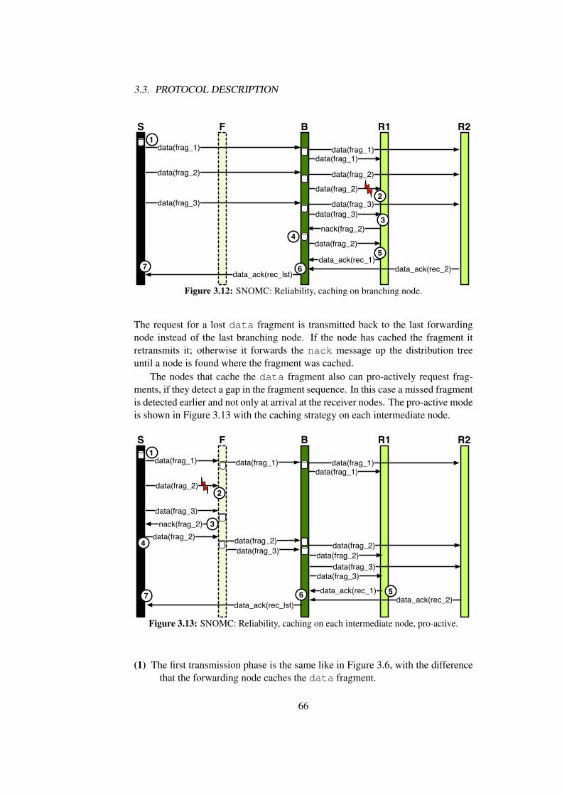
3.3. PROTOCOL DESCRIPTION
S B R1 R2
nack(frag_2)
data_ack(rec_2)
F
data(frag_1)
data_ack(rec_lst)
data(frag_1)data(frag_1)
data(frag_2)
data(frag_2)
data(frag_2)
data(frag_3)data(frag_3)
data(frag_3)
data(frag_2)
data_ack(rec_1)
1
2
3
5
6
4
7
Figure 3.12: SNOMC: Reliability, caching on branching node.
The request for a lost data fragment is transmitted back to the last forwardingnode instead of the last branching node. If the node has cached the fragment itretransmits it; otherwise it forwards the nack message up the distribution treeuntil a node is found where the fragment was cached.
The nodes that cache the data fragment also can pro-actively request frag-ments, if they detect a gap in the fragment sequence. In this case a missed fragmentis detected earlier and not only at arrival at the receiver nodes. The pro-active modeis shown in Figure 3.13 with the caching strategy on each intermediate node.
S B R1 R2
nack(frag_2)
data_ack(rec_2)
F
data(frag_1)
data_ack(rec_lst)
data(frag_1)data(frag_1)
data(frag_2)
data(frag_3)
data(frag_2)data(frag_2)
data(frag_2)
data_ack(rec_1)
1
2
3
56
4
data(frag_1)
data(frag_2)data(frag_3)
data(frag_3)data(frag_3)
7
Figure 3.13: SNOMC: Reliability, caching on each intermediate node, pro-active.
(1) The first transmission phase is the same like in Figure 3.6, with the differencethat the forwarding node caches the data fragment.
66

3.4. CONCLUSIONS
(2) A data fragment gets lost.
(3) The forwarding node detects the loss when the third data fragment arrivesand requests pro-actively the missed second fragment. It does not forwardfragment 3 in order to preserve the sequence of the fragments. The for-warding node then generates a nack message (cf. Figure 3.14(a)), which istransmitted towards the sender node.
(4) Since the previous node in the distribution tree has the fragment in the cache,it retransmits it towards the requesting forwarding node. After receiving theretransmitted fragments the forwarding node transmits fragments 2 and 3 tothe next node towards the receivers.
(5)-(7) The last three steps (data acknowledgement) are the same like in the previ-ous caching strategies.
If sensor node that requests a missed fragment starts also a retransmissiontimer. If the retransmission timer expires and the requested fragment does notarrived, the sensor node requests the fragment again.
To ensure end-to-end reliability we are using two types of messages, the nackmessage (shown in Figure 3.14(a) and the data ack message shown in Figure3.14(b). While the nack message is used for requesting missed fragments, thedata ack message is used to acknowledge the successful receive of all fragmentsat the end of the transmission (not of each fragment). The nack message containsthe field type with the value nack, and further the field rec lst with the listof the receivers. It also contains the field frag no with the list of the missedfragments. The message data ack contains also the field type with the valuedata ack and the list of the receivers, which successfully received all fragments(field rec lst).
type frag_norec_lst
(a) nack message
type rec_lst
(b) data ack mes-sage
Figure 3.14: SNOMC: reliability messages.
3.4 Conclusions
This chapter introduced the Sensor Node Overlay Multicast (SNOMC) protocol,which is specifically designed for overlay multicast transport in wireless sensornetworks. It supports a reliable dissemination of bulky data from one sender nodeto many receiver nodes.
A distribution tree is used to transmit the data efficiently from the sender nodeto the receiver nodes using overlay connections. We described the joining phase,
67

3.4. CONCLUSIONS
which results in a distribution tree, composed of one sender node, forwardingnodes, branching nodes, and the receiver nodes. The overlay connections are UDPflows between the sensor nodes and are described in Section 4.3.4. As an opti-mization we introduced a broadcast transmission at the branching nodes to avoidunnecessary unicast transmissions to two ore more following nodes.
To ensure end-to-end reliability we designed a NACK-based reliability mech-anism, combined with a data acknowledgement after the successful transmissionof all data fragments to the receiver nodes. To avoid costly end-to-end retransmis-sions we propose different caching strategies: caching on each intermediate node,caching on branching nodes, or only caching on the sender node. Further, the nodeswhich cache data also can pro-actively request missing fragments.
The following chapter 4 presents the SNOMC implementation in the OM-NeT++ simulator and a real-world implementation in the Contiki OS. A quanti-tative evaluation of SNOMC is further presented in chapter 5.
68

Chapter 4
SNOMC Implementation
This chapter describes the implementation details of SNOMC. After a short intro-duction in Section 4.1, we describe the implementation details of SNOMC in theOMNeT++ simulator [9] in Section 4.2 and the implementation in the Contiki OS[38] in Section 4.3. Finally, a concise summary is given in Section 4.4.
4.1 Introduction
SNOMC was designed as a multicast transport protocol to perform efficient man-agement tasks in MARWIS. Before integrating the two we decided to indepen-dently evaluate SNOMC. In order to make a proper performance evaluation wetook the two-step approach.
First, for a proof-of concept evaluation we implemented SNOMC in the OM-NeT++ simulator. Later, for real-world experiments in the Wisebed testbed and theintegration in MARWIS, we implemented SNOMC in the Contiki OS.
4.2 SNOMC Implementation in OMNeT++
In this section we describe the implementation of SNOMC in the OMNeT++ sim-ulator. SNOMC has been implemented in the INET framework provided by OM-NeT++. The INET framework is suited for simulations of wired, wireless andad-hoc networks. Beyond IP and UDP/TCP there are implementations of 802.11,Ethernet, PPP, IPv6, OSPF, RIP, and several other protocols.
In this section, first the OMNeT++ protocol stack is described. Afterwards,we describe the implementation of the protocol operations of SNOMC and theimplementation of CC2420 radio transceiver. Moreover, the implementation ofimportant SNOMC data structures and messages is discussed.
4.2.1 Protocol Stack
OMNeT++ is very appropriate for the evaluation of complex systems. Figure4.1 shows the OMNeT++ protocol stack. Our protocol stack covers the applica-
69

4.2. SNOMC IMPLEMENTATION IN OMNET++
tion, SNOMC, UDP, µIP, NullMAC and ContikiMAC as MAC protocols and theCC2420 radio.
APP
SNOMC
UDP
uIP
CONTIKIMAC NULLMAC
RADIO
NotificationBoard
Interface Table
Routing Table
Channel Control
Network
Figure 4.1: OMNeT++: protocol stack.
The application module is responsible to start the joining phase and later thedata transmission. After finishing the data transmission it collects statistically datasuch as transmission time. The SNOMC protocol has been implemented as a statemachine, which is described detailed in Section 4.2.2. The UDP module is takenunchanged from the OMNET++ INET framework. The µIP module is adaptedfrom the original IP module, provided by the INET framework. All functionalityto fragment packets are removed - in method fragmentAndSend(), because themaximum size of a fragment is fixed to 78 (due to of the MTU of 802.15.4 MAC-FRAMES of 128 Bytes). Since, we only want to support overlay multicast themethod for routing multicast packets is removed (routeMulticastPacket()).
As MAC protocols we implemented NullMAC and ContikiMAC, which areintegral part of Contiki OS. The description of the protocols can be found in Section2.6.
The CC2420 radio transceiver is implemented in the class CC2420Radio.The state machine (shown in Figure 4.5 and described in Section 4.2.3) is imple-mented as a class CC2420RadioState and the states are defined as enums, suchas CC2420 IDLE, CC2420 TX CAL, or CC2420 SLEEP. The transitions be-tween the states are implemented as method calls, such as setRadioToIDLE(),setRadioToTX CAL(), or setRadioToSLEEP(). Some transitions are ini-tiated by the upper MAC protocol via commands (such as STXON or SRXON).Autonomous state transitions (such as TX CAL → TX Preamb Send → TXSend) are handled via timers which expire according the state transition dura-
70

4.2. SNOMC IMPLEMENTATION IN OMNET++
tions in the real CC2420 radio transceiver. The timers are handled as self mes-sages via handleSelfMessages(). There are two buffers, one for incom-ing messages called RX Buffer, and one for outgoing messages called TX Buffer.To empty the RX Buffer and the TX Buffer the methods flushRXBuffer()and flushTXBuffer() are used. When a frame arrives at the radio it is de-livered by the ChannelControl module. After finishing the receiving processthe radio transmits the command RECEPTION COMPLETE which initiates pro-cessing of the handleLowerMsgEnd() method. Within this method the frameis handled - if there is a collision (handleCollision()), if there is a bit er-ror (handleBiterror()), or the frame received correctly (handleCorrectFrame()). In the latest case, the frame is written in the RX Buffer.
There are a number of global modules, such as notificationBoard, theinterfaceTable as well as the routingTable. Using the notificationBoard all protocol layers can exchange information. Thus, a module is able to no-tify that one of their values or states have changed. When a change occurs, the mod-ule has to post the change using the method fireChangeNotification().Every other module that wants to be notified about a change can subscribe tothe notificationBoard using the method subscribe(). The module hasto be a child from the class INotifiable. The subscribed module gets no-tified when the function receiveChangeNotification() is called. TheinterfaceTable contains all interfaces such as the radio or serial interface.The routingTable contains all routes between the sensor nodes. The ChannelControl module includes the radio model and calculates with the help of param-eter, such as bitrate, bandwidth, carrier frequency, modulation, thermal noise, radiosensitivity, and other parameter the signal-to-noise ratio (SNR) of a signal at the re-ceiving node. Further, the ChannelControlmodule delivers the received frameto the radio module of the node, if there is no bit error or collision.
4.2.2 Protocol Operation
The SNOMC protocol has been implemented in OMNeT++ as a state machines.Depending on whether the node acts as a sender node, a receiver node, or a for-warding/branching node the state machine differs.
Figure 4.2 shows the simplified state machine of the sender node. When itstarts the joining procedure it creates the join message, checks the receiver listand sends the message to the according neighbour. Then it waits for incomingjoin ack messages. When such a message arrives, it checks if all receivers havenotified the joining to the multicast group. If this is not the case, the sender nodestays in the waiting for join acks state. If all join ack messages ar-rived, the data transmission procedure starts. The data gets fragmented, the frag-ments are buffered and packed into the data messages and transmitted to theaccording neighbour. Afterwards, the sender node waits for next events. Whena nack message arrives, it creates a data message with the requested fragmentand transmits it to the according neighbour. When a data ack message arrives, it
71

4.2. SNOMC IMPLEMENTATION IN OMNET++
join_ack
yes
nack
start joining
create "join"send "join"
wait for join_acks
all received?
start data transmission
no fragment "data"buffer "data"send "data"
wait for event
retransmit "data"
all received?
data_ack
transmission finished
yesno
Figure 4.2: OMNeT++: SNOMC state machine, sender node.
checks, if all receivers acknowledged the successful data transmission. If this is notthe case, it goes back to the wait for event state. If all data ack messagesarrived, the data transmission finished successfully.
wait for event
process "join"prepare buffer
join
send "nack"start "nack_timer"
data
missed frags?
no
yes
buffer "data"
transmissionfinished
send "data_ack"
nack_timer
Figure 4.3: OMNeT++: SNOMC state machine, receiver nodes.
Figure 4.3 shows the simplified state machine of the receiver node. The onlystate is the wait for event state. The behaviour of the receiver depends onthe incoming messages. When a join message arrives, the receiver processes it,defines its own role as a receiver and prepares the buffer for the incoming datamessages. Afterwards, it goes back to the wait for event state. When adata message arrives the receiver node buffers it and checks if fragments aremissing. If so, a nack message is created and transmitted towards the sendernode. Afterwards, a nack timer is started and the state machine goes back tothe wait for event state. When the nack timer expires, again the buffer ischecked for missed fragments. If fragments are missing the timer is started again.If all fragments have successfully arrived the receiver a data ack message is senttowards the sender node and the transmission is finished.
72

4.2. SNOMC IMPLEMENTATION IN OMNET++
wait for event
process "join"forward "join"
join
process "join_ack"forward "join_ack"
join_ack
forward "data"
data
cache? no
cache "data"
yes
cached?nack
forward "nack"
no
retransmit "data"
yes
forward "data_ack"
data_ack
Figure 4.4: OMNeT++: SNOMC state machine, forwarding/branching nodes.
Figure 4.4 shows the simplified state machine of a forwarding/branching node.The behaviour of both node types does not differ much. A forwarding node hasonly to forward a message to one neighbour while a branching node has to forwardthe message to two or more neighbours. The state machine has only one state,the wait for event state. When a join message arrives the node decides onits role (as a forwarding or branching node) and the message is forwarded to thenext neighbour. Similar is the behaviour when a join ack message arrives. Themessage gets processed and forwarded towards the sender node. When a datamessage arrives the behaviour depends on the caching strategy. If the node doesnot cache fragments, the message is just forwarded. If the node caches fragments,the fragment is cached before the message is forwarded. When a nack messagearrives, the behaviour also depends on the caching strategy. If the requested frag-ment is cached on the node, the fragment is taken from the buffer and transmitted asdata message to the requesting receiver. If this is not the case, the nack messageis transmitted towards the sender node.
4.2.3 CC2420 Radio
Figure 4.5 shows the state machine of a CC2420 radio transceiver as it was im-plemented in the CC2420Radio class. The radio transceiver has two buffers,one for outgoing messages (RX Buffer) and one for incoming messages (TXBuffer). Each of them stores 128 bytes. The radio transceiver is realized as abuilt-in state machine, which is used to switch between different operational states.The change of state is done either by using commands or by internal events suchas SFD (Start Frame Delimiter). The CC2420 provides an AUTO-ACK mode. An
73

4.2. SNOMC IMPLEMENTATION IN OMNET++
Frame TX Acknowledge TX
Frame RX
TXCAL IDLE RX
CALACKSend
TXPreamb
SendSFD
SearchACK
PreambSend
TXSend RECV ACK
CAL
STXON SRXON
SRFOFF
STXON
SACK
SACKOverflow
Auto ACKdisabled SFD
found
RXOverflow
1 2
3
45
8
7
6
9
10
11
Figure 4.5: OMNeT++: CC2420 state machine.
acknowledgement frame is transmitted for all incoming frames accepted by theaddress recognition with the acknowledge request flag set and a valid CRC. Theaddress recognition is part of the CC2420 transceiver.
The red transitions are commands, the black ones are internal events. The statesare numbered as follows:
(1) In the IDLE state the radio is switched off. If the MAC protocol gives theSTXON or SRXON command the radio transceiver switches to the corre-sponding state.
(2) The frequency synthesizer has to be calibrated to receive the frames. Thiscalibration (RX CAL) takes 192 µs. Afterwards, the radio transceiver switchesto the SFD Search state.
(3) In the SFD Search state the radio transceiver listens for the SFD byte (Startof Frame Delimiter). If the SFD is found the radio transceiver switches tothe RECV state. If the MAC protocol transmits a SACK (Send Acknowl-edge) command, the radio transceiver switches to the ACK CAL state. If theradio transceiver receives a SRFOFF command, it disables the receiving/-transmission of messages and the frequency synthesizer and switches to theIDLE state.
(4) The radio transceiver receives the frame. If the RX buffer overflows, thenext state is the RX Overflow. If the AUTO-ACK flag is disabled, it returnsto the SFD Search state. Otherwise, the radio transceiver sets the SACKcommand and thus switches to the ACK CAL state.
(5) If there is an overflow (RX Overflow), the RX buffer is emptied (by MAC
74
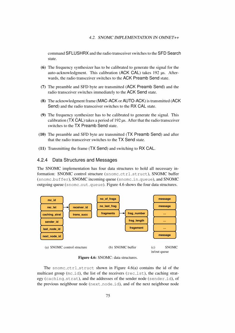
4.2. SNOMC IMPLEMENTATION IN OMNET++
command SFLUSHRX and the radio transceiver switches to the SFD Searchstate.
(6) The frequency synthesizer has to be calibrated to generate the signal for theauto-acknowledgment. This calibration (ACK CAL) takes 192 µs. After-wards, the radio transceiver switches to the ACK Preamb Send state.
(7) The preamble and SFD byte are transmitted (ACK Preamb Send) and theradio transceiver switches immediately to the ACK Send state.
(8) The acknowledgment frame (MAC-ACK or AUTO-ACK) is transmitted (ACKSend) and the radio transceiver switches to the RX CAL state.
(9) The frequency synthesizer has to be calibrated to generate the signal. Thiscalibration (TX CAL) takes a period of 192 µs. After that the radio transceiverswitches to the TX Preamb Send state.
(10) The preamble and SFD byte are transmitted (TX Preamb Send) and afterthat the radio transceiver switches to the TX Send state.
(11) Transmitting the frame (TX Send) and switching to RX CAL.
4.2.4 Data Structures and Messages
The SNOMC implementation has four data structures to hold all necessary in-formation: SNOMC control structure (snomc ctrl struct), SNOMC buffer(snomc buffer), SNOMC incoming queue (snomc in queue), and SNOMCoutgoing queue (snomc out queue). Figure 4.6 shows the four data structures.
last_node_id
sender_id
caching_strat
rec_lst
mc_id
next_node_id
receiver_id
trans_succ
(a) SNOMC control structure
fragments
no_of_frags
frag_number
frag_length
fragement
no_last_frag
(b) SNOMC buffer
…
message
message
…
…
message
(c) SNOMCin/out queue
Figure 4.6: SNOMC: data structures.
The snomc ctrl struct shown in Figure 4.6(a) contains the id of themulticast group (mc id), the list of the receivers (rec lst), the caching strat-egy (caching strat), and the addresses of the sender node (sender id), ofthe previous neighbour node (next node id), and of the next neighbour node
75

4.3. SNOMC IMPLEMENTATION IN CONTIKI OS
(next node id). The list of receivers is realized as a STL (Standard Tem-plate Library) list. Each entry of the list contains the address of the receiver(receiver id) and a flag if the receiver successfully received all data (transsucc).
The snomc buffer shown in Figure 4.6(b) contains all buffered data frag-ments. It contains the total number of cached fragments (no of frags), the se-quence number of the last fragment (no last frag), and a list of the fragments(fragments). The list of cached fragments is realized as a STL list. Each entryof the fragment list contains the sequence number (frag number) and the lengthof the fragment (frag length) and the data of the fragment (fragment). TheSNOMC buffer has the same structure on the sender node, the receiver node andall nodes that cache the data.
The queues of the incoming packets and the outgoing packets have the samestructure and are shown in Figure 4.6(c). They are also realized as a STL list andcontain any kind of messages. It is organized as a FIFO queue so that the messagesstay in the same order.
The SNOMC messages are also realized as C++ classes. The fields of eachmessage are attributes of this class. Additional information and parameters can beattached to the message using the addPar function. The message handling is doneusing the functions handleMessage, handleLowerMessage, handleUpperMessage, and handleSelfMessage, depending on from which layerthe message arrives. The following SNOMC messages have been implemented:join, join ack, data, data ack, and nack. The messages are described inSection 3.3 and shown in the Figures 3.3, 3.5, 3.10, and 3.14.
4.3 SNOMC Implementation in Contiki OS
In this section we present details of the SNOMC implementation in Contiki OS.In contrast to the implementation in the OMNeT++ simulator the implementationtook a bigger effort, because we had to solve many challenges regarding the limi-tations of the sensor nodes and the operating system. We implemented the sender-driven mode and the three caching strategies, including pro-actively requestingmissed fragments.
First, we describe the joining and the data transmission procedure on the im-plementation level. The procedures are depicted using flowcharts, which are bettersuited for intuitive presentation than pseudo-code listings. Afterwards we showimplementation details of the caching, the packet queues, the SNOMC sender andcontrol process, timers and variables.
4.3.1 Joining Procedure
Figure 4.7 shows the joining procedure on the sender node. It depicts the start ofthe joining procedure and the behaviour when a join ack messages receives the
76

4.3. SNOMC IMPLEMENTATION IN CONTIKI OS
has received from all receivers?
start joining
wait for event
receive"join_ack" message
yes
startdata
transmission
no
Sender Node
3
4
start "join_ack"timer
5
send "join" message (s)
to neighbour(s)
creates "join"message(s)
checks receivers list
1
2
"join_ack" timer expires
6
Figure 4.7: SNOMC control process: joining procedure, sender node.
sender node.
(1) The sender node starts the joining procedure. First, it checks the receivers listand the routing table and decides via which neighbour nodes the receiverscan be reached. Afterwards, it creates the join message(s) and transmitsthem to the neighbours accordingly.
(2) Then, it starts the join ack timer and awaits the next event.
(3) When the sender node receives a join ackmessage, it checks if it got it fromall receivers.
(4) If it did not get the notifications from all receivers it restarts the join acktimer again and waits for the next event.
(5) If it got the notifications from all receivers the joining procedure is finishedand the data transmission can start.
(6) When the join ack timer expires it checks in the receiver list which re-ceivers have not notified the joining in the multicast group. Then, the proce-dure continuous with step (1).
Figure 4.8 shows the joining procedure for the forwarding nodes, branchingnodes, and receiver nodes. Initially, the nodes will be not know which role theywill play and which caching strategy is used.
(1) The node receives the join message. First, it checks the receiver list in thejoin message and define its own role as follows. If all receivers can bereached via one single neighbour node, it acts as a forwarding node. If thereceivers can be reached via different neighbour nodes, it acts as a branchingnode.
77

4.3. SNOMC IMPLEMENTATION IN CONTIKI OS
receive"join"
message
wait for event
receive"join_ack" message
no
Forwarding Node
Branching Node
Receiver Node
am I receiver?
do I cachefragments?
send "join" message(s)
to neighbour(s)
prepare buffer
no
nostart
"data_reception"timer
am I branching
node?
has received from all receivers?
(re)start "join_ack"timer
wait for event
yes
yes
no
yes
forward "join_ack"message towards
the sender
combine "join_ack" messages
yes
2
45
6
7
8
9
10
checks receivers list
1
3
11
"join_ack" timer expired
Figure 4.8: SNOMC control process: joining procedure, other nodes.
(2) Then, it checks in the join message which caching strategy is used. If thenode has to cache the data fragments it prepares the buffer. If not, it continueswithout the buffer preparation.
(3) In the receiver list of the join message the node sees if it is a receiver nodeor not.
(4) If it is a receiver node, it starts the data reception timer and waits forthe next events.
(5) If the node is not on the receivers list, it just forwards the join message to theone or more neighbour nodes (depending on whether the node is a branchingnode or a forwarding node). Then, it waits for the next event.
(6) When the node receives a join ack message, it checks first its own role.
(7) If the node is a forwarding node it just forwards the join ack message to-wards the sender node.
(8) If the node is a branching node, it checks if it got notifications from all receivernodes.
(9) If it got all notifications, it combines these notifications to a new join ackmessage and forwards it towards the sender node.
(10) If not all notifications from all receivers have arrived the node starts thejoin ack timer and waits for incoming events.
(11) When the join ack timer expires, it checks if all notifications arrived inthe meanwhile and the procedure continuous with step (8).
78

4.3. SNOMC IMPLEMENTATION IN CONTIKI OS
4.3.2 Data Transmission Procedure
has received from all receivers?
start data transmission
buffer "data" fragments
receive "nack"
message
receive"data_ack" message
yes
wait for event
Sender Node
1
forward "data" message
to neighbor(s)
"data_ack"timer expires
no
yes
data transmitted
all "data" fragments in the
buffer send?
start "data_ack"
timer
take "data" fragment from
buffer
wait for event
mark all data fragments in
buffer as unsent
restart "data_ack"
timer
no
2
3
4
5
6
7
8
9fragment datacreate "data"
messages
Figure 4.9: SNOMC control process: data transmission, sender node.
After the joining procedure the data transmission procedure starts. Figure 4.9shows the procedure for the sender node. The sender node is responsible for thefragmentation of the data and for the transmission to the receiver nodes. The datatransmission is finished when all receivers are notified that all data arrived success-fully.
(1) As first step of the data transmission procedure the data has to be fragmented.This procedure is described in detail in Section 4.3.3. Then, the data frag-ments are stored in the buffer. In the beginning all data fragments in thebuffer are marked as unsent.
(2) A standard check up is made, if all data fragments in the buffer were sent. Inthe first check after the initial data fragmentation clearly no data fragmenthas been sent so far.
(3) If all fragments were sent, the data ack timer is started and the processwaits for the next events.
(4) If not all fragments are sent, the next unsent fragment is taken from the bufferand forwarded to the next neighbour(s). Afterwards, the procedure continueswith step (2).
(5) If a nack message arrives at the sender node, the requested missed fragmentwill be taken from the buffer and transmitted to the neighbour(s). Since thesender node created the fragments, it has all of them in the buffer for sure. Itis also independent of the caching strategy, because the sender node anywaycaches all fragments.
79

4.3. SNOMC IMPLEMENTATION IN CONTIKI OS
(6) If a data ack message arrives the sender node this means that one or morereceivers successfully got all data fragments. The sender node checks if itgot notification from all receivers.
(7) If it got a notification from all receivers, the data transmission finished suc-cessfully.
(8) If it does not got a notification from all receivers, the data ack timer isrestarted and the sender node waits for next events.
(9) The expiration of the data ack timermeans that the data transmission wasnot successful to all receivers or a subset of them. In this case all fragmentsin the buffer are marked as unsent and the data will be retransmitted to allreceiver nodes. The procedure starts again with step (2).
"nack" timer expires
yes
no
send "data_ack" message
towards sender
deliver data tothe application
receive"data"
message
buffer "data" fragment
wait for event
1
are "data" fragments missed?
Send "nack" message with
missed fragments
Receiver Node
(re)start "nack" timer
2
3
4
5
6
"data_reception" timer expires
create "join_ack" message
send "join_ack" message towards
the sender
restart "data_reception"
timer
7
Figure 4.10: SNOMC control process: data transmission, receiver nodes.
Figure 4.10 shows the situation at the receiver nodes. The receiver node getsthe data fragments and they request missed fragments. When all data fragmentshave arrived the receiver notifies the sender node about this.
(1) When the receiver node gets a data message with a data fragment it buffersit in its buffer.
(2) Then, the receiver node checks, if there are missed fragments.
(3) If this is not the case, the receiver notifies the sender node about this by trans-mitting a data ack message.
(4) After processing case (3), the receiver reassembles the data, deliver it to theapplication and waits for next events.
80

4.3. SNOMC IMPLEMENTATION IN CONTIKI OS
(5) If the receiver did not get all fragments, it creates a nack message with themissed fragments and forwards it towards the sender node. Then, it (re)startsthe nack timer and waits for new events.
(6) When the nack timer expires the receiver node checks again which frag-ments are missing. The procedure continuous with step (2).
(7) The data reception timer is started after the join message received(cf. Figure 4.8). If data only consists of one fragment and this fragment getslost, the receiver node cannot know if there is any data transmission after thejoining procedure. This timer ensures that the receiver node does not waitinfinitely after the joining procedure. When the data reception timerexpires a second join ack message is generated and transmitted towardsthe sender node. Afterwards, the data reception timer is restarted.
receive"data_ack" message
receive"nack"
message
yes
no
combine different "nack"
messages
Forwarding Node
Branching Node
forward "data_ack"message towards
sender node
receive"data"
message
forward fragment(s)
to neighbour(s)
wait for event
wait for event
am I branching
node?
duplicate "data" message
yes
no
do I cachefragments?
do I have the fragment?
yes
forward "nack"
message
no
am I branching
node
yes
no
"nack_wait" timer expires
5
6
7 8
13
do I cachefragments?
cache fragment
1
yes
no
2
3
4
9
11
10
12
wait for event
take "data" fragment
from buffer
send "data" fragment to
receiver
store "nack"
message
start "nack_wait"
timer
14
15
Figure 4.11: SNOMC control process: data transmission, other nodes.
Figure 4.11 shows the situation at the forwarding and branching nodes. Bothnodes are responsible for forwarding of data messages, for caching, and for re-transmission of missed fragments.
(1) When a node receives a data message it first checks, if it should cache thedata, depending on the role of the node and the selected caching strategy.
(2) If yes, the node stores the data fragment in the buffer, if it is not already cached(in case the data message was a retransmission).
(3) If it should not cache the data (according to the caching strategy), it just con-tinues with the procedure.
(4) Next, the node checks if it is a branching node.
81

4.3. SNOMC IMPLEMENTATION IN CONTIKI OS
(5) If it is a branching node it duplicates the data message and forwards it totwo or more neighbour nodes. If the broadcast optimization is enabled thebranching node broadcasts the data message.
(6) If the node is a forwarding node, it forwards the data message with the du-plication and waits for further events.
(7) When the node receives a data ack message, it forwards the message to-wards the sender node.
(8) When a nack message arrives, the node first checks if it generally shouldcached fragments, depending on the role of the node and the selected cachingstrategy.
(9) If the node should not cache fragments, it only forwards the nack messagetowards the sender node.
(10) If the node does caching it checks the requested fragment is in the buffer.
(11) If the fragment is in the buffer, then it copies the fragment from the buffer andsends it to the requesting receivers.
(12) If the node does not have the requested fragment in the buffer, the nodesfurther behaviour depends on whether the node is a forwarding node or abranching node.
(13) If it is a forwarding node it only forwards the nack message towards thesender node.
(14) If it is a branching node it stores the nack message and waits for certain time(nack wait timer) for further nack messages to combine them.
(15) When the nack wait timer expires it checks if in the meanwhile othernackmessages arrived. It combines them and forwards the combined nackmessage towards the sender node.
When the node pro-actively requests missed fragments it checks if fragmentsare missed in its own buffer and pro-actively requests the missed fragments. Theprocedure is the same as shown in Figure 4.10, numbers (2) to (5).
4.3.3 Fragmentation, Caching, and Buffer
The fragmentation of data of 1000 bytes into smaller fragments of 70 bytes each isaccomplished by the function buildFragment(uint8 t size). This func-tion builds a data message (fragment) with a given size. Afterwards, this functionstores the fragment in the buffer.
To implement the cache discussed in Section 3.3.2, a simple buffer was imple-mented as cache. The caching strategy is defined in the snomc ctrl struct
82

4.3. SNOMC IMPLEMENTATION IN CONTIKI OS
shown in Figure 4.6(a). All types of nodes (sender node, forwarding nodes, branch-ing nodes, receiver nodes) have the same buffer implementation. The structure ofthe buffer is called buffer t and includes, besides the storage of the fragments,also information about the number of fragments (no of frags) and the numberof the last fragment (no last frag). The size of the memory is dynamically al-located using the Managed Memory Allocator (mmem) provided from Contiki OS.The structure of the buffer is depicted in Figure 4.12.
no_of_frags
no_last_frag
fragments…
…
Figure 4.12: Buffer structure.
To cache a fragment, an intermediate node simply copies the frag field of thedata message to the right position in the cache buffer. This position in the cachebuffer is characterized by a start byte, which is calculated from the size of thefragment and the frag no.
4.3.4 SNOMC Control/Sender Process and Packet Queues
As discussed in Section 2.6, the µIP TCP/IP stack of Contiki OS uses a singlebuffer for incoming and outgoing messages. Therefore, µIP does not have a queuefor incoming or outgoing packets and only one packet is stored. Thus, packet lossalso happens because the sensor node can not store an incoming packet while theµIP buffer is occupied, since the processing of the current packet is not finishedand µIP does not overwrite the global packet buffer. That is problematic, sincedue to the preconfigured backoff time of the MAC protocol, a node waits beforeit actually transmits a packet. During this time period, the node is not able toreceive new packets. To overcome this issue we implemented the SNOMC protocolas four Contiki processes: SNOMC control process (described above) with theincoming packet queue process and the SNOMC sending process with the outgoingpacket queue process. Both packet queues act as proxies between the SNOMCcontrol/sender processes and µIP. Thus, the SNOMC control/sender processes donot talk directly to µIP, instead they use the packet queues for receiving new packetsand transmitting packets.
The SNOMC sending process is shown in Figure 4.13. The SNOMC senderprocess does not transmit a message directly via the µIP buffer. Instead, it adds the
83

4.3. SNOMC IMPLEMENTATION IN CONTIKI OS
send message
wait for event
"packet_send" timer expires
SNOMC Sender Process
start "packet_send" timer
add message to out_packet_queue
1
2
take first message from
out_packet_queue
send message
restart "packet_send"
timer
wait for event
uIP buffer occupied?
message stays in out_packet_queue
4
3
56
yes
no
Figure 4.13: SNOMC sender process: sending messages
message to the outgoing packet queue (out packet queue). The out packetqueue is polled frequently by the SNOMC sender process (randomly between
20ms and 84ms) and the first message in the queue is send.
(1) When SNOMC wants to send a message, it does not simply send it via the µIPbuffer. It stores the message in the outgoing packet queue (out packetqueue). The queue is in fact a FIFO queue, the first packet stays on the firstposition. Thus, the order of the packets is ensured.
(2) After storing the packet, the packet send timer is started. Then, the pro-cess waits for next events.
(3) When the packet send timer expires, the first packet is taken from theout packet queue.
(4) Then it is checked, whether the µIP buffer is free.
(5) If the buffer is free, the message is sent. Afterwards the packet send timeris restarted.
(6) If the buffer is occupied the packet stays in the out packet queue and thepacket send timer is restarted.
The outgoing packet queue is implemented using managed memory alloca-tor provided by the Contiki OS. Thus, we have a dynamic sized queue. TheSNOMC sender process uses the function addToQueue(* msg) to add a packetto the queue. Since, the queue is organized as a FIFO memory, the functiongetFromQueue() always returns the first (and oldest) packet of the queue.
Figure 4.14 shows the interaction between the SNOMC control process and theincoming packet queue .
84

4.4. CONCLUSIONS
initialize
wait for typ_ip event
tcp_ip event arrives
SNOMC Control Process
attach to queue
1copy packet from
uIP buffer to in_packet_queue
post packet_event
wait for event
3
2
Figure 4.14: SNOMC control process: receiving messages
(1) First, the process of the communication protocol has to tell the incoming packetqueue that it wants to use the queue. The process does that by executing theattachToQueue(handle h) function. This function stores the processID of the process of the SNOMC receiver process in the data structure h oftype handle. Next, the attachToQueue function starts the incomingpacket queue process, which is listening for tcp ip events posted by µIP.
(2) If new packets arrive, µIP posts the tcp ip event, signalling that a new packetwas copied into the global packet buffer. The packet queue now checks fora free packet slot.
(3) If so, the new packet in the global packet buffer is copied to this slot, otherwise,the packet is dropped. The packet queue now posts the packet queueevent to the process with the ID stored in the data structure handle. Thereceiver process of the SNOMC protocol has to listen for the event packetevent. If such an event arrives, the process uses the getPacket functionto access the new packet. This function returns a pointer to the data of thenew packet.
4.4 Conclusions
This chapter focussed on the details of the SNOMC implementation in the OM-NeT++ simulator and in the Contiki OS. Based on the SNOMC design describedin Chapter 3 we implemented SNOMC for both platforms. The protocol operationsare implemented as state machines. The behaviour depends on the state and the in-coming message. Due to the limitations of the µIP buffer incoming and outgoingmessages are queued in two separate queues. An important property of SNOMCis caching, which is implemented using a buffer structure. In OMNeT++ we addi-tionally implemented the underlying MAC protocols NullMAC and ContikiMACand the CC2420 radio transceiver.
With these two implementations of SNOMC we had the possibility to makea proper performance evaluation of SNOMC against other popular data dissemi-
85

4.4. CONCLUSIONS
nation protocols as well as the possibility to integrate SNOMC in the MARWISarchitecture. This integration allows us to perform management tasks such as codeupdate, reconfiguration and monitoring in an efficient way. This has been evaluatedin Chapter 8.
The following Chapter 5 presents the quantitative evaluation of SNOMC. Tomake a proof-of-concept evaluation we first use the implementation in the OM-NeT++ simulator. Later, to determine its performance in a real-world environmentwe use the Contiki OS implementation in the Wisebed testbed.
86
Chapter 5
SNOMC Evaluation
In this section we evaluate the SNOMC (Sensor Node Overlay Multicast) protocoland compare its performance against a number of other data dissemination proto-cols for wireless sensor networks, such as Flooding, MPR (Multipoint Relay) [90],PSFQ (Pump Slowly, Fetch Quickly) [129], TinyCubus [73], and Directed Diffu-sion [59, 60]. For a detailed description of the protocols we refer to Section 2.6.Additionally, we compared it to two unicast protocols, namely UDP and TCP.
After Introduction in Section 5.1 we present the results of the evaluation usingthe OMNeT++ simulator in Section 5.2. The evaluation of SNOMC in the Wisebedtestbed is presented in Section 5.3. Section 5.4 compares the simulated results andthe results of the real-worlds experiments. Section 5.5 concludes this chapter.
5.1 Introduction
The performance of SNOMC in terms of transmission time, number of totallytransmitted packets and energy consumption is compared to other data dissemina-tion protocols often used in wireless sensor networks. We chose broadcast-basedprotocols such as Flooding, MPR (Multipoint Relay), and TinyCubus. Further-more, we consider typical data dissemination protocols especially designed forwireless sensor networks, such as PSFQ (Pump Slowly, Fetch Quickly), and Di-rected Diffusion. Since we are using Contiki OS, which supports a µIP protocolstack, we also compare SNOMC to the unicast-based distribution using UDP andTCP.
We implemented the above protocols in the OMNeT++ simulator and madeevaluations to proof the general concepts of the SNOMC protocol, such as join-ing procedure, data transmission, reliability mechanisms, and the different cachingstrategies. Later, we implemented them in Contiki OS to evaluate SNOMC underreal-world conditions running experiments in the Wisebed testbed.
To ensure a fair evaluation we implemented on top of each of the protocols(except for TCP) a simple NACK-based reliability mechanism including differentcaching strategies as used in SNOMC. Furthermore, we used SNOMC on top ofdifferent MAC protocols to show the performance of SNOMC, independently of
87

5.2. SNOMC EVALUATION OF SIMULATION RESULTS
the underlying MAC protocol. In the OMNeT++ implementation we used BEAM[13, 122], and implementations of NullMAC and ContikiMAC, which are inte-grated in the Contiki OS. The latter two we used for our real-world experiments inthe Wisebed testbed. We could not use BEAM for the real-world experiments, be-cause the BEAM implementation in Contiki OS does not support broadcast trans-missions.
5.2 SNOMC Evaluation of Simulation Results
This section presents the evaluation of the SNOMC protocol in the OMNeT++simulator. First, we describe the protocol stack. Then, we introduce the differentsimulation scenarios. Finally, we discuss the results of our measurements.
5.2.1 Protocol Stack
To evaluate the performance of SNOMC, we compare it to a number of data dis-semination protocols commonly found in wireless sensor networks in combinationwith different underlying MAC protocols. More specifically, these protocols are:Flooding, Multipoint Relay, TinyCubus, Directed Diffusion, UDP, and TCP as datadissemination protocols as well as BEAM [13], ContikiMAC [33] and NullMACas MAC protocols. For the description of the protocols we refer to Section 2.6.All protocols have been implemented in the OMNeT++ simulator [9]. The pro-tocol stack is shown in Fig. 5.1 and is based on the µIP stack from Contiki OS.To enable a fair comparison we had to ensure end-to-end reliability for all proto-cols and implement the same simple NACK-based reliability mechanism as usedin SNOMC.
PHY / 802.15.4
NULLMAC
μIP
TCP
APP
SNOMC
BEAM
E2E
UDP FLOOD MPR TinyCubus
DirectedDiffusion
CONTIKIMAC
Figure 5.1: Simulation protocol stack.
The underlying MAC protocol plays an important role for the transmissionof data between neighbour nodes. Hence, different MAC protocols can lead tosignificantly different results, irrespectively of the used transport or multicast pro-tocol. We chose three MAC protocols with different support mechanisms for reli-ability and energy-efficient operation. The Burst-aware Energy-Efficient AdaptiveMAC Protocol (BEAM) [13] uses an adaptive duty cycle mechanism, which reacts
88

5.2. SNOMC EVALUATION OF SIMULATION RESULTS
Table 5.1: MAC Protocol Parameters.
acknowledgements max. retransmissions energy-savingBEAM positive ack 5 yes
ContikiMAC early ack 2 yesNullMAC no 0 no
quickly to changes in both traffic loads and traffic patterns and ensures hop-to-hopreliability. ContikiMAC [33], which is part of the Contiki operating system, alsosupports energy-saving radio duty cycling mechanisms and reliability based onan acknowledgement mechanism. NullMAC, also part of Contiki, has no energy-saving mechanisms and does not support reliability. Table 5.1 shows an overviewof the parameter of the used MAC protocols.
5.2.2 Simulation Scenarios
We arranged 36 sensor nodes in a grid of 6x6 nodes with a distance of 100 metersbetween each two nodes as shown in Fig. 5.2. Since we are interested in a multicastscenario, we chose a sender (node 0) with three receivers (node 17, 33, and 35).
6 7 8 9 10 11
12 13 14 15 16 17
18 19 20 21 22 23
24 25 26 27 28 29
30 31 32 33 34 35
0 1 2 3 4 5
(a) SNOMC
6 7 8 9 10 11
12 13 14 15 16 17
18 19 20 21 22 23
24 25 26 27 28 29
30 31 32 33 34 35
0 1 2 3 4 5
(b) UDP and TCP
6 7 8 9 10 11
12 13 14 15 16 17
18 19 20 21 22 23
24 25 26 27 28 29
30 31 32 33 34 35
0 1 2 3 4 5
(c) Directed Diffusion
6 7 8 9 10 11
12 13 14 15 16 17
18 19 20 21 22 23
24 25 26 27 28 29
30 31 32 33 34 35
0 1 2 3 4 5
(d) Flooding
6 7 8 9 10 11
12 13 14 15 16 17
18 19 20 21 22 23
24 25 26 27 28 29
30 31 32 33 34 35
0 1 2 3 4 5
(e) MPR
6 7 8 9 10 11
12 13 14 15 16 17
18 19 20 21 22 23
24 25 26 27 28 29
30 31 32 33 34 35
0 1 2 3 4 5
(f) TinyCubus
Figure 5.2: Simulation scenarios.
89

5.2. SNOMC EVALUATION OF SIMULATION RESULTS
Table 5.2: Simulation Parameters.
carrierFrequency bit-rate sensitivity thermalNoise TX power modulation2.4 GHz 250 kbps -94 dBm -110 dBm 1mW O-QPSK
Table 5.3: Energy Consumption of the CC2420 Radio Transceiver.
mode sleeping receiving transmittingconsumption in mA 0.4 mA 18.8 mA 17.4 mA
Given the chosen simulation scenario, each of the compared protocols affectsa different set of nodes. In case of SNOMC there are two branching nodes (21, 28)and three forwarding nodes (7, 14, 22) as shown in Fig. 5.2(a). For UDP and TCPthe same nodes are affected but there are three independent unicast connections(cf. Figure 5.2(b)). As shown in Fig. 5.2(c) a different set of nodes participates inthe distribution tree in Directed Diffusion, which is a result of the different Interestmessage routing compared to the static routing of SNOMC. In Flooding all nodesare affected (cf. in Fig. 5.2(d)). In the chosen grid scenario the Multipoint Relayprotocol calculates a rather high number of multipoint relay nodes (cf. Fig. 5.2(e)).In the case of TinyCubus, the same set of nodes as in SNOMC is affected. Due todesign decisions the protocol does not distinguish between receivers and interme-diate forwarders (cf. Fig. 5.2(f)). Hence, all nodes in the set (7, 14, 21, 22, and 28)will rebroadcast the packets.
We created two evaluation scenarios, which differ in the size of the transmittedmessages - 20 bytes and 1000 bytes. The size of 1000 bytes is typically associ-ated with software updates on the sensor nodes; the size of 20 bytes is related to ashort configuration message for the sensor nodes. For each scenario, 50 simulationruns are used for evaluation. We measured three parameters: (i) transmission timesfrom the sender to all receivers (including the joining phase), (ii) the total numberof packets it takes to ensure the successful reception of the data by all receivers, and(iii) the energy consumption of the nodes in the network. The energy consumptionis measured according to the CC2420 state machine with real state switching timesand energy consumption according to [120] and [83] (values for sleeping, receiv-ing, and transmitting, see Table 5.3) and is calculated per node and per transmittedbyte. The energy consumption of the CPU and writing the flash memory is muchsmaller than the energy consumption of the radio transceiver. Therefore, only theenergy consumption of the radio transceiver is taken into account.
In order to get realistic simulation results a radio model in OMNeT++ is im-plemented according to the data CC2420 manual [120] and the Castalia Simula-tor [83]. It is used to calculate the signal to noise ratio (SNR) based on parametersshown in Table 5.2. Using the SNR and real measurements with a CC2420 radiotransceiver the bit error rate (BER) is calculated. In addition, a packet error rate of
90

5.2. SNOMC EVALUATION OF SIMULATION RESULTS
5% is assumed to represent random noise and external interferences.
5.2.3 Transmission Times
In this section, we present our findings on transmission times. In all figures on thex-axis the combinations of transport and MAC protocols are shown. In our notationB stands for BEAM, C for ContikiMAC, and N for NullMAC.
First, in Fig. 5.3(a), we discuss results for the time required to transmit 1000bytes from the sender node to the three receiver nodes. SNOMC requires the short-est time to transmit 1000 bytes to the receivers. As expected, unicast data distri-bution based on UDP-E2E requires more time due to the redundant unicast flowsthat need to be established for each of the three receiver nodes. TCP performseven worse since every packet has to be acknowledged. This kind of traffic patterncaused by simultaneous data and acknowledgements increases collision probabil-ity and hence affects delay negatively. Flooding, Multipoint Relay, and TinyCubusare all broadcast protocols and are much worse in performance. On the one hand,broadcasting affects usually more nodes, which leads to a higher number of trans-missions. Consequently, the probability of collisions increases and more retrans-missions are necessary, pushing delay up. On the other hand, to avoid collisionshigher random back-off times are necessary compared to unicast-based protocols.This leads to longer transmission times.
Further we can see that using caching in intermediate nodes performs betterthan caching only on sender node. It avoids long end-to-end transmissions, whichcost time. Further, it reduces the number of packets in the network, which reducesthe probability of collisions.
0
5
10
15
SNOMCB|C|N
FLOODB|C|N
MPRB|C|N
TinyCubusB|C|N
DDB|C|N
UDP-E2EB|C|N
TCPB|C|N
time
[s]
protocol combinations
Transmission time (data distribution only) 1000 bytes
caching on sender nodecaching on intermediate nodes
caching on branching nodes (SNOMC only)
(a) 1000 bytes
0
0.2
0.4
0.6
0.8
SNOMCB|C|N
FLOODB|C|N
MPRB|C|N
TinyCubusB|C|N
DDB|C|N
UDP-E2EB|C|N
TCPB|C|N
time
[s]
protocol combinations
Transmission time (data distribution only) 20 bytes
caching on sender nodecaching on intermediate nodes
caching on branching nodes (SNOMC only)
(b) 20 bytes
Figure 5.3: Evaluation: transmission time.
Let us now compare the performance of the MAC protocols (BEAM, Contiki-MAC, NullMAC) in combination with the higher level transport protocols. In thediagrams, shown in Fig. 5.3(a), the MAC protocols are indicated with the letterunderneath the transport protocol name. In our notation B stands for BEAM, Cfor ContikiMAC, and N for NullMAC. We see that BEAM has a little worse per-formance than NullMAC (for SNOMC, Directed Diffusion, UDP-E2E and TCP).
91

5.2. SNOMC EVALUATION OF SIMULATION RESULTS
However, BEAM outperforms ContikiMAC, which is the result of two factors.First, BEAM is optimized for bulky traffic while ContikiMAC focuses only onconstant (or slowly changing) traffic. Bulky traffic is characterised by transmis-sions of a large number of packets within a short time period. Second, BEAM [13]has better congestion control and duty cycle mechanisms. The latter is also the rea-son why caching at intermediate nodes affects the performance of both protocolsdifferently, i.e., for BEAM the effect is much smaller than for ContikiMAC. Null-MAC in combination with broadcast-based protocols (Flooding, MPR, TinyCubus)works better than BEAM in combination with these protocols. Since BEAM hasenergy-saving mechanisms, the radio transceiver can be in sleep mode. If so, longertime is needed to transmit a packet from sender to receiver. On the contrary, the ra-dio transceiver in NullMAC is always on and therefore the sender can immediatelytransmit the packet.
In case of 20 bytes of data a single packet has to be transmitted. Transmissiontimes are shown in Fig. 5.3(b). We see that SNOMC achieves the best perfor-mance. Ideally, TinyCubus requires a smaller number of transmissions comparedto SNOMC (due to using broadcast transmissions). SNOMC, however, has the ad-ditional benefit of smaller random-back off times (see implementation of the packetqueues in Section 4.3.4). UDP and TCP need more transmissions and longer trans-mission times due to the three independent flows. Due to just one packet has tobe transmitted in scenario 2, also TCP requires only one acknowledgement forthe transmitted packet, explaining the much smaller differences between TCP andUDP compared to the scenario with 1000 bytes.
Further, in SNOMC, TinyCubus, Directed Diffusion and UDP collisions amongdata and acknowledgements generally do not occur and hence no retransmissionsare required. Therefore, the corresponding boxplots in Fig. 5.3(b) are quite com-pact and do not have big outliers. Finally, the differences between Flooding, Mul-tipoint Relay and Directed Diffusion are similar as for the 1000 bytes scenario.
5.2.4 Number of Transmissions
Fig. 5.4(a) shows the number of total transmissions needed for the successful trans-fer of 1000 bytes. As we can see, SNOMC requires the fewest number of pack-ets, followed by UDP, TCP and Directed Diffusion. The results of broadcast-basedprotocols (Flooding, Multipoint Relay, and TinyCubus) are considerably worse andare compliant with our observations on transmission times. Flooding requires mosttransmissions (inherent to its communication style), followed by Multipoint Relay(result of the disadvantageous set of multipoint relays) and, with the best perfor-mance of the three, TinyCubus.
Looking at the MAC protocols, BEAM requires more packets to ensure hop-to-hop reliability than NullMAC, irrespectively of the transport protocol. This is dueto the fact that the receiver can be in sleeping mode and multiple attempts may berequired before the packet is transmitted successfully. ContikiMAC always needsmore packet retransmissions on link layer due to a worse duty cycle mechanism
92

5.2. SNOMC EVALUATION OF SIMULATION RESULTS
compared to the adaptive duty cycle mechanisms of BEAM. Thus, a higher numberof necessary end-to-end retransmissions on the transport layer is required.
0
500
1000
1500
2000
2500
3000
3500
SNOMCB|C|N
FLOODB|C|N
MPRB|C|N
TinyCubusB|C|N
DDB|C|N
UDP-E2EB|C|N
TCPB|C|N
sent
pac
kets
[#]
protocol combinations
Number of sent packets (data distribution only) 1000 bytes
caching on sender nodecaching on intermediate nodes
caching on branching nodes (SNOMC only)
(a) 1000 bytes
0
50
100
SNOMCB|C|N
FLOODB|C|N
MPRB|C|N
TinyCubusB|C|N
DDB|C|N
UDP-E2EB|C|N
TCPB|C|N
sent
pac
kets
[#]
protocol combinations
Number of sent packets (data distribution only) 20 bytes
caching on sender nodecaching on intermediate nodes
caching on branching nodes (SNOMC only)
(b) 20 bytes
Figure 5.4: Evaluation: number of transmitted packets.
The results for the transmission of 20 bytes are shown in Fig. 5.4(b). Tiny-Cubus achieves the best performance in combination with NullMAC. It has anoptimal set of forwarding nodes and NullMAC keeps the radio transceiver alwaysawake. Hence, this combination reaches the minimal number of packets (6) to en-sure the successful transmission of 20 bytes. The other broadcast protocols (Flood-ing and Multipoint Relay) show an improved performance as well, considering thescenario with 1000 bytes. Just one packet has to be transmitted, which causes lesscollisions and retransmissions. Out of all non-broadcast-based protocols, SNOMChas the best performance while Directed Diffusion has the worst. Directed Diffu-sion requires a larger number of packets because of the more extensive hop con-nectivity, i.e., more connections compared to UDP and TCP. If Directed Diffusionwould use the same sensor nodes as, e.g., UDP or TCP, it would perform better.Further, the differences between the three caching modes are quite small, a resultof the smaller number of required retransmissions.
5.2.5 Energy Consumption
We now discuss the energy consumed per node and per transmitted byte. Resultsfor the scenario with 1000 bytes are shown in Fig. 5.5(a). We compare only theperformance of BEAM and ContikiMAC, since NullMAC does not have an energysaving mechanism. In general, it can be seen that for broadcast-based protocolsthere is a stronger relation between the consumed energy and the number of trans-mitted bytes. More specifically, the more bytes are transmitted the higher is theenergy consumption per byte due to higher packet loss. The energy consumptionof unicast-based protocols is generally good with the exception of Directed Diffu-sion, which performs rather poor due to additional maintenance messages, e.g., forpath reinforcement or the propagation of new interest. Concerning the impact ofthe MAC protocol, BEAM offers higher energy-efficiency than ContikiMAC sincethe latter has a worse duty cycle mechanism compared to the adaptive duty cycle
93

5.3. SNOMC EVALUATION IN REAL-WORLD TESTBED
mechanism of BEAM. Furthermore, caching does not significantly influence theperformance of broadcast-based protocols from an energy point of view.
0
0.1
0.2
0.3
0.4
0.5
0.6
0.7
SNOMCB|C
FLOODB|C
MPRB|C
TinyCubusB|C
DDB|C
UDP-E2EB|C
TCPB|C
ener
gy [n
J] p
er B
yte
protocol combinations
Energy per Byte (all nodes, data distribution) 1000 bytes
caching on sender nodecaching on intermediate nodes
caching on branching nodes (SNOMC only)
(a) 1000 bytes
0
0.1
0.2
0.3
0.4
0.5
0.6
0.7
SNOMCB|C
FLOODB|C
MPRB|C
TinyCubusB|C
DDB|C
UDP-E2EB|C
TCPB|C
ener
gy [n
J] p
er B
yte
protocol combinations
Energy per Byte (all nodes, data distribution) 20 bytes
caching on sender nodecaching on intermediate nodes
caching on branching nodes (SNOMC only)
(b) 20 bytes
Figure 5.5: Evaluation: energy consumption per node and per transmitted byte.
In Fig. 5.5(b) corresponding results on energy consumption are shown for thescenario with a single packet (20 bytes). Due to the transmission of 20 bytes im-plies a lower number of collisions and retransmissions, the energy consumption pertransmitted byte is lower for 20 bytes (1 packet) than for 1000 bytes (15 packets).
5.3 SNOMC Evaluation in Real-World Testbed
In this section we present the results of the evaluation under real-world condi-tions. We measure the transmission time, the number of transmitted packets andthe consumed energy transmitting 1000 bytes from one sender node to three re-ceiver nodes.
For the evaluation we are using our in-house testbed developed in the Wisebedproject. It consists of 40 TMoteSky sensor nodes, which are distributed in thebuilding of the Institut fur Informatik und angewandte Mathematik. More detailedinformation about Wisebed can be found in Section 2.3.
First, the used protocol stack is described. Afterwards, we show the threeused evaluation scenarios followed by the measurements for time consumption,transmitted packets, and energy consumption.
5.3.1 Protocol Stack
To evaluate the performance of SNOMC, we compare it to a number of data dis-semination protocols commonly found in wireless sensor networks in combina-tion with different underlying MAC protocols. In addition to the implementa-tion and evaluation in OMNeT++ we implemented with PSFQ (Pump Slowly,Fetch Quickly) protocol another transport protocol. Moreover, we do not eval-uate SNOMC and the other data dissemination protocols with the BEAM MACprotocol. The reason is that BEAM implemented in Contiki OS does not support
94

5.3. SNOMC EVALUATION IN REAL-WORLD TESTBED
PHY / 802.15.4
NULLMAC
μIP
TCP
APP
SNOMC E2E
UDP FLOOD MPR TinyCubus
DirectedDiffusionPSFQ
CONTIKIMAC
Figure 5.6: Real-World protocol stack.
broadcast transmissions, which is necessary for the broadcast-based protocols andthe broadcast optimization of SNOMC.
Thus, the used protocols for the evaluation of SNOMC are: Flooding, Multi-point Relay, TinyCubus, PSFQ, Directed Diffusion, UDP, and TCP in combinationwith NullMAC and ContikiMAC. For the description of the protocols we refer toSection 2.6. All protocols have been implemented in Contiki OS [38]. The pro-tocol stack is shown in Fig. 5.6 and is based on the µIP stack from Contiki OS.To ensure a fair comparison with SNOMC, we also implemented in the real-worldevaluation the same simple NACK-based reliability mechanism, used in SNOMC,on top of all data dissemination protocols (except for TCP).
5.3.2 Experimentation Scenarios
For the evaluation of SNOMC we used three different scenarios in the in-housetestbed . The first scenario, shown in Figure 5.7, consists of all 40 sensor nodesin the in-house testbed. We have one sender node (number 7), and three receivernodes (numbers 16, 19, and 21). The SNOMC distribution tree spans over thenodes 4, 40, 23, and 1. The rest of the nodes are passive in transmitting the datausing SNOMC but they play an active role while transmitting data using Floodingor Multipoint Relay.
Since most of the broadcast-based protocols did not terminate and thus failedin scenario 1 with all 40 nodes (cf. Section 5.3.3), we choose a second scenario(see Figure 5.8). This scenario has the same sender node, the same receiver nodes,and the same spanned distribution tree for SNOMC. But it does not include all theother passive sender nodes. This leads to much less traffic and transmitted packetsusing the broadcast-based protocols and a better performance.
The third scenario, shown in Figure 5.9 is used to compare SNOMC specifi-cally with UDP-E2E. The sender node is again node number 7, but receiver node16 changed to receiver node 21. Thus also the spanned distribution tree changedand consists of the nodes number 4, 40, and 1. This scenario shows the advantagesof a multicast-based data distribution scheme compared to a unicast-based one.
95

5.3. SNOMC EVALUATION IN REAL-WORLD TESTBED
02
03
05
06
07
09
08
10
11
12
13
14
16
17
15
18
20
24
25
26 27
39
28
29
30
31 32
33
34 35
36
37
38
22
01
04
19
21
23
40
Figure 5.7: Evaluation scenario 1.
5.3.3 Transmission Times
In this section we present the results for the transmission time in the three scenarios.In all figures on the x-axis the combinations of data dissemination protocols withthe different caching strategies are shown. In our notation s stands for caching onlyon sender node, b(-pa) for caching on branching nodes (with pro-active request),i(-pa) caching on each intermediate sensor node (with pro-active request), and i-bcstands for the broadcast optimization of SNOMC. With pro-active mode each in-termediate node that caches data, requests actively missing fragments. Caching onbranching nodes and the broadcast optimization appears only in SNOMC. The dia-grams on the left side show the measured values using NullMAC, and the diagramon the right side shows the values using ContikiMAC. Both diagrams have the samescale on the y-axis to ease the comparison between NullMAC and ContikiMAC.
Figure 5.10(a) shows the transmission times transmitting 1000 bytes from onesender node to the three receiver nodes using NullMAC. Compared to the otherprotocols SNOMC has the best performance.
Only the performance of UDP-E2E comes close to SNOMC. Broadcast-basedprotocols such as Flooding and MPR work generally worse than unicast-based pro-tocols except for TCP. The reason is obvious. All packets (data as well as nackmessages) are broadcasted which leads to a huge amount of messages in the net-work and causes high interferences. The three broadcast-based protocols differ in
96

5.3. SNOMC EVALUATION IN REAL-WORLD TESTBED
01
04
07
11
1619 24
23
40
Figure 5.8: Evaluation scenario 2.
how many sensor nodes rebroadcast the packets. Therefore, Flooding has the worstperformance, followed by MPR, and TinyCubus. In case of using TinyCubus onlythe sensor nodes 4, 40, 23, and 1 rebroadcast the packets. Thus, there is less trafficin the network and TinyCubus performs better.
Directed Diffusion does not work and does not deliver results. The reason isthat the found paths are always very bad and in combination with the bad links thereare no stable connections. TCP performs poorly because each packet is acknowl-edged, and not only the missed one, leading to higher traffic and interferences.
Comparing the various caching strategies, we see that caching on each inter-mediate nodes show the best results. In case of SNOMC caching on each inter-mediate node performs better than caching on branching nodes. Thus, we cansay that the more often the packets are cached the better the performance is. Pro-actively requesting missed packets results on higher packet traffic in the network.Thus, always caching with pro-active requests has a worse performance comparedto caching strategies without pro-active requests.
If we have a look on Figure 5.10(b), we see the results using ContikiMAC. Asmentioned above, we see that a number of protocols does not work in this scenario.Only SNOMC, UDP-E2E, TinyCubus and partly Flooding show meaningful resultsat all. The other protocols fail. The reason is how ContikiMAC handles broadcasts.In the unicast case ContikiMAC sends a frame and gets back an acknowledgement.
97

5.3. SNOMC EVALUATION IN REAL-WORLD TESTBED
02
03
05
06
07
09
08
10
11
12
13
14
16
17
15
18
20
23
25
26 27
39
28
29
30
31 32
33
34 35
36
37
38
22
01
19
21
24
04
40
Figure 5.9: Evaluation scenario 3.
If the neighbour sleeps then there is no acknowledgement. ContikiMAC sends theframe until the neighbour wakes up and answers. In the broadcast case there are noacknowledgements. Hence, ContikiMAC sends as long as for the maximum dutycycle among the neighbours so that it can be ensured that every neighbour wasawake during this time. This produces a huge amount of traffic and interferences.
Figures 5.10(c) and 5.10(d) show the results transmitting 20 bytes from onesender to the receiver nodes using NullMAC and ContikiMAC respectively. Theresults are similar to the 1000 byte scenario. SNOMC has a smaller advantagecompared to UDP-E2E and TCP because the joining phase takes additional timebefore the delivery of the data can start. Using NullMAC (see Figure 5.10(c))the transmission times are lower than the transmission times using ContikiMAC(see Figure 5.10(d)). Directed Diffusion also does not deliver results using bothNullMAC and ContikiMAC, because it was not possible to establish stable routesin this scenario.
Since Directed Diffusion and PSFQ have phases in the protocol operation thatuse broadcast transmission, also theses protocols fail using ContikiMAC as MACprotocol. Therefore, we run the same experiments on a smaller scenario, whichonly consists of a sub-set of nodes, namely only 9 instead of 40. The results areshown in Figure 5.11.
Figure 5.11(a) shows the results using NullMAC. The results from SNOMC,
98

5.3. SNOMC EVALUATION IN REAL-WORLD TESTBED
0
100
200
300
400
500
600
700
800
s|b|b-pa|i|i-pa|i-bcSNOMC
s|i|i-paFLOOD
s|i|i-paMPR
s|i|i-paTinyCubus
s|i|i-paPSFQ
s|i|i-paDD
s|i|i-paUDP TCP
time
[s]
protocol
Comparing transmission time 1000 bytes nullmac
(a) NullMAC, 1000 bytes
0
100
200
300
400
500
600
700
800
s|b|b-pa|i|i-pa|i-bcSNOMC
s|i|i-paFLOOD
s|i|i-paMPR
s|i|i-paTinyCubus
s|i|i-paPSFQ
s|i|i-paDD
s|i|i-paUDP TCP
time
[s]
protocol
Comparing transmission time 1000 bytes CONTIKIMAC
(b) ContikiMAC, 1000 bytes
0
10
20
30
40
50
60
70
s|b|b-pa|i|i-pa|i-bcSNOMC
s|i|i-paFLOOD
s|i|i-paMPR
s|i|i-paTinyCubus
s|i|i-paPSFQ
s|i|i-paDD
s|i|i-paUDP TCP
time
[s]
protocol
Comparing transmission time 20 bytes nullmac
(c) NullMAC, 20 bytes
0
10
20
30
40
50
60
70
s|b|b-pa|i|i-pa|i-bcSNOMC
s|i|i-paFLOOD
s|i|i-paMPR
s|i|i-paTinyCubus
s|i|i-paPSFQ
s|i|i-paDD
s|i|i-paUDP TCP
time
[s]
protocol
Comparing transmission time 20 bytes CONTIKIMAC
(d) ContikiMAC, 20 bytes
Figure 5.10: Evaluation: transmission time, scenario 1.
UDP-E2E, and TCP are almost the same as in the large 40-node scenario, becausethe same set of nodes are affected as in scenario 1. We can see that SNOMCoutperforms all protocols.
Also in this smaller scenario 2 broadcast-based protocols such as Flooding,MPR, and TinyCubus perform poor. The reasons are still the same as in scenario1. A lot of packets in the network leading to high interferences and thus manyretransmissions. Directed Diffusion and PSFQ perform better than the broadcast-based protocols. Directed Diffusion finds good paths in the interest phase to deliverthe data efficiently.
Also the results in this scenario show that the caching strategy has significantinfluence. Caching only on the sender node performs worse than caching on eachintermediate node and pro-active requests of missing packets cause worse perfor-mance due to higher traffic and more interferences.
While most of the data dissemination protocols failed in scenario 1 using Con-tikiMAC, we have results for all of them in scenario 2, as shown in Figure 5.11(b).SNOMC outperforms all other protocols, broadcast-based protocols perform worst,and the different caching strategies have a certain influence. If we look at the broad-cast optimization of SNOMC we see the strong influence of the underlying MACprotocol. In combination with NullMAC the broadcast optimization performs verywell. It shows the overall best performance of all protocol and caching combina-
99

5.3. SNOMC EVALUATION IN REAL-WORLD TESTBED
0
50
100
150
200
250
300
s|b|b-pa|i|i-pa|i-bcSNOMC
s|i|i-paFLOOD
s|i|i-paMPR
s|i|i-paTinyCubus
s|i|i-paPSFQ
s|i|i-paDD
s|i|i-paUDP TCP
time
[s]
protocol
Comparing transmission time 1000 bytes nullmac
(a) NullMAC, 1000 bytes
0
50
100
150
200
250
300
s|b|b-pa|i|i-pa|i-bcSNOMC
s|i|i-paFLOOD
s|i|i-paMPR
s|i|i-paTinyCubus
s|i|i-paPSFQ
s|i|i-paDD
s|i|i-paUDP TCP
time
[s]
protocol
Comparing transmission time 1000 bytes CONTIKIMAC
(b) ContikiMAC, 1000 bytes
0
10
20
30
40
50
60
s|b|b-pa|i|i-pa|i-bcSNOMC
s|i|i-paFLOOD
s|i|i-paMPR
s|i|i-paTinyCubus
s|i|i-paPSFQ
s|i|i-paDD
s|i|i-paUDP TCP
time
[s]
protocol
Comparing transmission time 20 bytes nullmac
(c) NullMAC, 20 bytes
0
10
20
30
40
50
60
s|b|b-pa|i|i-pa|i-bcSNOMC
s|i|i-paFLOOD
s|i|i-paMPR
s|i|i-paTinyCubus
s|i|i-paPSFQ
s|i|i-paDD
s|i|i-paUDP TCP
time
[s]
protocol
Comparing transmission time 20 bytes CONTIKIMAC
(d) ContikiMAC, 20 bytes
Figure 5.11: Evaluation: transmission time, scenario 2.
tions. In combination with ContikiMAC the broadcast optimization has an oppositeimpact, since ContikiMAC handles broadcast transmissions inefficiently.
Figures 5.11(c) and 5.11(d) show the results transmitting 20 bytes in scenario2 using NullMAC and ContikiMAC respectively. The difference in performancebetween the broadcast-based protocols and both SNOMC and UDP-E2E is smallerin scenario 2 than in scenario 1, because just a small number of nodes are affected.Additionally, only one packet has to be transmitted which leads to less traffic andthus less packet loss and necessary retransmissions.
To have a comparison to the hardest competitor of SNOMC, UDP-E2E, wechoose a third scenario to compare both protocols. Figure 5.12 shows diagramswith the results using NullMAC and ContikiMAC. We see that SNOMC outper-forms UDP-E2E by factor of 2 to 2.5 with both MAC protocols due to the reducednumber of hops. With UDP-E2E at least 18 hops are necessary to transmit a packetto all three receiver nodes. In case of using SNOMC just 6 hops, or even 4 hopswith the broadcast optimization. Thus, we see the advantage of the overlay multi-cast communication scheme compared to a unicast-based one. UDP-E2E has verylow overhead, because it does not have a joining phase but the reduced number ofhops in the distribution tree compensates the joining overhead.
In both diagrams we again see the effect of the caching strategy and the effectof ContikiMAC for the broadcast optimization of SNOMC.
100

5.3. SNOMC EVALUATION IN REAL-WORLD TESTBED
0
20
40
60
80
100
120
140
s | b | b-pa | i | i-pa | i-bcSNOMC
s | i | i-paUDP
time
[s]
protocol
Comparing transmission time 1000 bytes NULLMAC
(a) NullMAC, 1000 bytes
0
20
40
60
80
100
120
140
s | b | b-pa | i | i-pa | i-bcSNOMC
s | i | i-paUDP
time
[s]
protocol
Comparing transmission time 1000 bytes CONTIKIMAC
(b) ContikiMAC, 1000 bytes
0
5
10
15
20
25
30
35
s | b | b-pa | i | i-pa | i-bcSNOMC
s | i | i-paUDP
time
[s]
protocol
Comparing transmission time 20 bytes NULLMAC
(c) NullMAC, 20 bytes
0
5
10
15
20
25
30
35
s | b | b-pa | i | i-pa | i-bcSNOMC
s | i | i-paUDP
time
[s]
protocol
Comparing transmission time 20 bytes CONTIKIMAC
(d) ContikiMAC, 20 bytes
Figure 5.12: Evaluation: transmission time, scenario 3.
5.3.4 Number of Transmissions
The number of transmissions is another metric that shows how efficiently a protocoloperates. The more packets are necessary to deliver a certain number of bytes themore inefficient is the protocol.
Figure 5.13 shows the number of transmitted packets with 1000 bytes fromone sender to three receivers. These are results for scenario 1 with the combina-tion of NullMAC or ContikiMAC. We can see that the broadcast-based protocolsrequire much more transmissions to deliver the data to the receivers compared tothe unicast-based protocols. SNOMC outperforms all other protocols also in thismetric.
Directed Diffusion, PSFQ, TCP, and partly TinyCubus, MPR and Flooding failin combination with ContikiMAC in scenario 1. In combination with NullMAConly Directed Diffusion fails.
Figures 5.13(c) and 5.13(d) show the results of transmitting 20 bytes in sce-nario 1. Also in the 20 bytes scenario the broadcast-based protocols require asignificantly large number of transmissions because the whole network with all 40nodes get flooded. In contrast to that, SNOMC and UDP-E2E just require a smallnumber of transmission to deliver the 20 bytes to the receivers. Just as in the 1000bytes scenario using ContikiMAC takes more necessary transmissions than usingNullMAC. The combination of NullMAC and Directed Diffusion fails also in this
101

5.3. SNOMC EVALUATION IN REAL-WORLD TESTBED
0
10000
20000
30000
40000
50000
60000
70000
s|b|b-pa|i|i-pa|i-bcSNOMC
s|i|i-paFLOOD
s|i|i-paMPR
s|i|i-paTinyCubus
s|i|i-paPSFQ
s|i|i-paDD
s|i|i-paUDP TCP
pack
ets
[#]
protocol
Comparing packets 1000 bytes NULLMAC
(a) NullMAC, 1000 bytes
0
10000
20000
30000
40000
50000
60000
70000
s|b|b-pa|i|i-pa|i-bcSNOMC
s|i|i-paFLOOD
s|i|i-paMPR
s|i|i-paTinyCubus
s|i|i-paPSFQ
s|i|i-paDD
s|i|i-paUDP TCP
pack
ets
[#]
protocol
Comparing packets 1000 bytes CONTIKIMAC
(b) ContikiMAC, 1000 bytes
0
2000
4000
6000
8000
10000
12000
14000
s|b|b-pa|i|i-pa|i-bcSNOMC
s|i|i-paFLOOD
s|i|i-paMPR
s|i|i-paTinyCubus
s|i|i-paPSFQ
s|i|i-paDD
s|i|i-paUDP TCP
pack
ets
[#]
protocol
Comparing packets 20 bytes NULLMAC
(c) NullMAC, 20 bytes
0
2000
4000
6000
8000
10000
12000
14000
s|b|b-pa|i|i-pa|i-bcSNOMC
s|i|i-paFLOOD
s|i|i-paMPR
s|i|i-paTinyCubus
s|i|i-paPSFQ
s|i|i-paDD
s|i|i-paUDP TCP
pack
ets
[#]
protocol
Comparing packets 20 bytes CONTIKIMAC
(d) ContikiMAC, 20 bytes
Figure 5.13: Evaluation: number of transmitted packets, scenario 1.
scenario, because Directed Diffusion was not able to stable stable routes.Therefore, we used scenario 2 with much less sensor nodes to evaluate the
protocols. The results are shown in Figure 5.14.SNOMC requires a somewhat lower number of transmissions than UDP-E2E.
SNOMC requires additional packets for the joining phase. It has a slight advantagein number of hops due to the use of a distribution tree instead of using three parallelunicast connections as UDP-E2E uses.
The broadcast-based protocols use a high number of transmissions due to broad-casting and rebroadcasting of the packets, although only a small number of ninenodes (see Figure 5.11) are rebroadcasting the packets. Directed Diffusion requiresmany packets in the Interest phase, which uses broadcast transmissions to find theadequate paths. Also PSFQ uses broadcast transmissions in its pump operation.
Comparing the two MAC protocols we see that ContikiMAC requires muchmore transmissions than NullMAC, especially for the broadcast-based protocols.The reason is how ContikiMAC handles broadcast transmissions. As describedin Section 2.6.1 ContikiMAC rebroadcast a packet for the full wake-up interval(128ms). We also see this effect comparing the SNOMC broadcast optimizationfor NullMAC and ContikiMAC.
Also the influence of the caching strategy can be seen in theses diagrams.Caching on the sender node requires end-to-end retransmissions of missed frag-
102

5.3. SNOMC EVALUATION IN REAL-WORLD TESTBED
0
5000
10000
15000
20000
25000
30000
35000
40000
s|b|b-pa|i|i-pa|i-bcSNOMC
s|i|i-paFLOOD
s|i|i-paMPR
s|i|i-paTinyCubus
s|i|i-paPSFQ
s|i|i-paDD
s|i|i-paUDP TCP
pack
ets
[#]
protocol
Comparing packets 1000 bytes NULLMAC
(a) NullMAC, 1000 bytes.
0
5000
10000
15000
20000
25000
30000
35000
40000
s|b|b-pa|i|i-pa|i-bcSNOMC
s|i|i-paFLOOD
s|i|i-paMPR
s|i|i-paTinyCubus
s|i|i-paPSFQ
s|i|i-paDD
s|i|i-paUDP TCP
pack
ets
[#]
protocol
Comparing packets 1000 bytes CONTIKIMAC
(b) ContikiMAC, 1000 bytes.
0
2000
4000
6000
8000
10000
s|b|b-pa|i|i-pa|i-bcSNOMC
s|i|i-paFLOOD
s|i|i-paMPR
s|i|i-paTinyCubus
s|i|i-paPSFQ
s|i|i-paDD
s|i|i-paUDP TCP
pack
ets
[#]
protocol
Comparing packets 20 bytes NULLMAC
(c) NullMAC, 20 bytes.
0
2000
4000
6000
8000
10000
s|b|b-pa|i|i-pa|i-bcSNOMC
s|i|i-paFLOOD
s|i|i-paMPR
s|i|i-paTinyCubus
s|i|i-paPSFQ
s|i|i-paDD
s|i|i-paUDP TCP
pack
ets
[#]
protocol
Comparing packets 20 bytes CONTIKIMAC
(d) ContikiMAC, 20 bytes.
Figure 5.14: Evaluation: number of transmitted packets, scenario 2.
ments, which leads to a high number of transmissions. The nack message has tobe transmitted from the receiver node to the sender node and the missed fragmenthas to retransmitted from the sender node back to the receiver node. If the missedfragment is cached on a branching or intermediate node, an end-to-end retransmis-sion is not required. Thus, caching on intermediate nodes (or branching nodes)decreases the number of hops (and transmissions) for a packet request.
Figures 5.14(c) and 5.14(d) show the results of transmitting 20 bytes in scenario2. The results are similar to the results of scenario 1 (see Figures 5.14(c) and5.14(d)). SNOMC and UDP-E2E requires significantly less transmissions thanFlooding, MRP and TinyCubus. Directed Diffusion and PSFQ perform as poor asthe broadcast-based protocols because both have protocol phases, which dependalso on broadcasts.
5.3.5 Energy Consumption
Energy consumption is measured for all nodes individually and is accumulated forthe whole network. Thus, in scenario 1 energy consumption of 40 nodes is mea-sured and accumulated. The consumed energy includes the energy for transmittingand receiving packets, the operation of the micro-controller on the sensor node,and reading/writing flash memory.
103

5.3. SNOMC EVALUATION IN REAL-WORLD TESTBED
0
100000
200000
300000
400000
500000
600000
s|b|b-pa|i|i-pa|i-bcSNOMC
s|i|i-paFLOOD
s|i|i-paMPR
s|i|i-paTinyCubus
s|i|i-paPSFQ
s|i|i-paDD
s|i|i-paUDP TCP
ener
gy [m
J]
protocol
Comparing energy 1000 bytes NULLMAC
(a) NullMAC, 1000 bytes.
0
100000
200000
300000
400000
500000
600000
s|b|b-pa|i|i-pa|i-bcSNOMC
s|i|i-paFLOOD
s|i|i-paMPR
s|i|i-paTinyCubus
s|i|i-paPSFQ
s|i|i-paDD
s|i|i-paUDP TCP
ener
gy [m
J]
protocol
Comparing energy 1000 bytes CONTIKIMAC
(b) ContikiMAC, 1000 bytes.
0
20000
40000
60000
80000
100000
s|b|b-pa|i|i-pa|i-bcSNOMC
s|i|i-paFLOOD
s|i|i-paMPR
s|i|i-paTinyCubus
s|i|i-paPSFQ
s|i|i-paDD
s|i|i-paUDP TCP
ener
gy [m
J]
protocol
Comparing energy 20 bytes NULLMAC
(c) NullMAC, 20 bytes.
0
20000
40000
60000
80000
100000
s|b|b-pa|i|i-pa|i-bcSNOMC
s|i|i-paFLOOD
s|i|i-paMPR
s|i|i-paTinyCubus
s|i|i-paPSFQ
s|i|i-paDD
s|i|i-paUDP TCP
ener
gy [m
J]
protocol
Comparing energy 1000 bytes CONTIKIMAC
(d) ContikiMAC, 20 bytes.
Figure 5.15: Evaluation: energy consumption, scenario 1.
Figure 5.15(a) shows the results in energy consumption using NullMAC. Since,NullMAC is an always on protocol (without any energy saving mechanisms) themeasured energy values behave as the transmission times - the faster the trans-mission of the 1000 bytes finishes, the less energy is needed for the transmission.Comparing the results using ContikiMAC (cf. Figure 5.15(b)), we again see that anumber of protocol combinations failed such as Directed Diffusion and PSFQ.
Figures 5.15(c) and 5.15(d) show the results in energy-consumption transmit-ting 20 bytes in scenario 1. Naturally, less energy is consumed transmitting just 20bytes than 1000 bytes. But the relation between the compared protocols is similarto the 1000 byte scenario. SNOMC requires less energy than the other protocols in-dependent of the underlying MAC protocol. Using NullMAC requires more energythan using ContikiMAC, because NullMAC has no energy-saving mechanisms.
Due to the problems in scenario 1 described in Section 5.3.2, we re-run theexperiments using scenario 2, with just 9 sensor nodes. The results are shown inFigure 5.16. Using ContikiMAC (cf. Figure 5.16(b)) leads to longer transmis-sion time but also to lower energy consumption. ContikiMAC uses duty cyclesas energy-saving mechanism so that the sensor node go to sleep when there isnothing to transmit or receive. The sensor nodes awake periodically and check ifthere is an incoming packet. Thus, considerable energy can be saved. The energy-consumption depends on the transmission time, the number of transmitted and re-
104

5.3. SNOMC EVALUATION IN REAL-WORLD TESTBED
0
20000
40000
60000
80000
100000
s|b|b-pa|i|i-pa|i-bcSNOMC
s|i|i-paFLOOD
s|i|i-paMPR
s|i|i-paTinyCubus
s|i|i-paPSFQ
s|i|i-paDD
s|i|i-paUDP TCP
ener
gy [m
J]
protocol
Comparing energy 1000 bytes NULLMAC
(a) NullMAC, 1000 bytes.
0
20000
40000
60000
80000
100000
s|b|b-pa|i|i-pa|i-bcSNOMC
s|i|i-paFLOOD
s|i|i-paMPR
s|i|i-paTinyCubus
s|i|i-paPSFQ
s|i|i-paDD
s|i|i-paUDP TCP
ener
gy [m
J]
protocol
Comparing energy 1000 bytes CONTIKIMAC
(b) ContikiMAC, 1000 bytes.
0
10000
20000
30000
40000
50000
60000
s|b|b-pa|i|i-pa|i-bcSNOMC
s|i|i-paFLOOD
s|i|i-paMPR
s|i|i-paTinyCubus
s|i|i-paPSFQ
s|i|i-paDD
s|i|i-paUDP TCP
ener
gy [m
J]
protocol
Comparing energy 20 bytes NULLMAC
(c) NullMAC, 20 bytes.
0
10000
20000
30000
40000
50000
60000
s|b|b-pa|i|i-pa|i-bcSNOMC
s|i|i-paFLOOD
s|i|i-paMPR
s|i|i-paTinyCubus
s|i|i-paPSFQ
s|i|i-paDD
s|i|i-paUDP TCP
ener
gy [m
J]
protocol
Comparing energy 1000 bytes CONTIKIMAC
(d) ContikiMAC, 20 bytes.
Figure 5.16: Evaluation: energy consumption, scenario 2.
ceived packets and the duty cycles of the sensor nodes.Saving energy using ContikiMAC works fine when we have mainly unicast
transmissions as in SNOMC, UDP, TCP, and partly Directed Diffusion and PSFQ.In these cases we save a lot of energy compared to using NullMAC (approximatelyby the factor of 2 to 3). For the broadcast-based protocols such as Flooding, MPRand TinyCubus we save less energy, explained by the way how ContikiMAC han-dles broadcast transmissions. It broadcasts packets for a time period of 128ms andduring this time the node does not go to sleep. Therefore, broadcast-based proto-cols using ContikiMAC save less energy (approximately by the factor of 1.5 to 2)than the other data dissemination protocols (SNOMC, UDP-E2E, TCP).
The results using NullMAC in scenario 2 are shown in Figure 5.16(a). SinceNullMAC does not save energy, the results for energy consumption correspond tothe results for transmission time.
Figures 5.16(c) and 5.16(d) show the results for transmitting 20 bytes in sce-nario 2. Also here we can see the expected results. SNOMC and UDP-E2E requireless energy than the other data dissemination protocols.
Summarizing the results of the experiments in the real-world testbed we cansee that SNOMC outperforms the other data dissemination protocols in terms oftransmission time, energy consumption, and number of transmitted packets in dif-ferent scenarios. SNOMC outperforms unicast-based protocols such as UDP-E2E
105

5.4. COMPARISON OF SIMULATED AND REAL-WORLD RESULTS
because it requires a lower number of hops to deliver the data. In big scenarioswith a large number of sensor nodes broadcast-based protocols such as Flooding,MPR, TinyCubus, and PSFQ perform very bad or even fail to transmit the data tothe receiver nodes. The energy consumption strongly depends on the underlyingMAC protocol. Using energy-saving ContikiMAC saves a lot of energy comparedto NullMAC. SNOMC performs very good independent of the underlying MACprotocol.
5.4 Comparison of Simulated and Real-World Results
Our main observation is that simulation results differ from the results of the real-world experiments. The reasons for that difference are mainly in the implementa-tion of the protocols in the OMNeT++ simulator.
One major aspect is the handling of the packet in the protocol stack. In OM-NeT++ all processing time of a packet in the protocol stack is zero. In ContikiOS the transfer of a packets through the several protocol layers from the radio tothe application layer takes a certain amount of time. Since Contiki OS uses pro-tothreads, processes can be interrupted and thus the processing time of packets candiffer a lot.
Another fact that causes difference in results is that broadcasting of Contiki-MAC was implemented in OMNeT++ in a different way compared to the imple-mentation in Contiki OS. In the OMNeT++ implementation it does not broadcastthe packets for a certain time period as in the Contiki OS implementation. Instead,in the OMNeT++ implementation ContikiMAC broadcasts a packet just three timesin a row as it is done in the OMNeT++ implementation of NullMAC. This fact alsocauses difference between simulations results and the results of the real-world ex-periments.
Although, in OMNeT++ a realistic radio model was implemented to gain real-istic results, our experiments using testbed showed that in reality interferences havea much higher impact on transmissions. Additional external interferences are takeninto account in the implementation of the radio model but no effect such as reflec-tion or multi-path fading. Due to the in-house testbed is located in the institutesbuilding this effects occur regularly and influence the results strongly.
There are some differences among the scenarios. The distance between thethe sensor nodes in the simulation scenarios is much higher than in the in-housetestbed scenarios. Therefore, on the in-house testbed, due to more overlappinginterference ranges, transmitted packets experience higher collision probabilities.This is especially the case for broadcast-based protocols. To avoid these problemsseveral timers such as the retransmission timer, random back off timer, etc, in theContiki OS implementation were given much higher values compared to ones inthe OMNeT++ implementation.
Beside the differences between the simulation results and the real-world re-sults we have also commonalities. The relation in the results between the different
106

5.5. CONCLUSIONS
protocols in the simulation and in the real-world experiments are similar. We cansee that in both evaluation environments broadcast-based protocols perform muchworse than the other protocols. SNOMC performs always best independent of ofthe underlying MAC protocol.
The main advantage of the evaluation of SNOMC in the OMNeT++ simulatoris that it allows an easy implementation of the protocol and thus a fast proof-of-concept. The main advantage of the evaluation of SNOMC in Wisebed is that ithelps to optimize the protocol for real-world environments.
5.5 Conclusions
We propose the Sensor Node Overlay Multicast (SNOMC) protocol to supporta reliable, time-efficient and energy-efficient dissemination of bulky data fromone sender node to many receivers. To ensure end-to-end reliability we designedand implemented a NACK-based reliability mechanism. Further, to avoid costlyend-to-end retransmissions we propose different caching strategies implementedin SNOMC.
In this chapter we evaluated SNOMC against a number of data disseminationprotocols for wireless sensor networks, such as Flooding, MPR (Multipoint Re-lay), PSFQ (Pump Slowly, Fetch Quickly), TinyCubus, and Directed Diffusion aswell as the unicast-based protocols UDP and TCP. To ensure a fair competitionwe implemented the same reliability mechanisms and caching strategies on top ofthe selected protocols. As underlying MAC protocols we chose BEAM, Contiki-MAC and NullMAC for the simulations, and ContikiMAC and NullMAC for thereal-world evaluation.
As proof-of-concept of SNOMC we made an evaluation in the OMNeT++ sim-ulator. For evaluating the performance of SNOMC in real-world we run a numberof experiments in our in-house Wisebed testbed. We choose three performancemetrics: transmission time, number of transmitted packets and energy consump-tion.
We showed that the SNOMC protocol performs very well compared to theselected data dissemination protocols. Especially, broadcast-based data dissemi-nation protocols, such as Flooding, MPR, and TinyCubus cause broadcast stormsand thus perform very poor. Data dissemination protocols especially designed forwireless sensor networks, such as Directed Diffusion or PSFQ, have some protocolphases also relying on broadcast transmissions. Thus, also these protocols performworse than SNOMC. The most serious competitor of SNOMC is UDP-E2E. In thiscase the advantage of SNOMC depends on the topology of the network and thedistribution tree as we showed in Section 5.3.3. Especially in scenario 3 SNOMCshows its advantage compared to UDP-E2E, because the forks in distribution treeare close to the receivers.
Further, we showed the influence of the different caching strategies. In general,we can say that caching on intermediate nodes improves the performance of each
107

5.5. CONCLUSIONS
protocol, since expensive end-to-end retransmissions are avoided. We also showedthat pro-active requesting of missed fragments does not improve the performanceat all. Pro-active requesting causes additional packets, higher traffic and thus muchmore collisions, which cancels the advantage of the intended optimization.
Moreover, we showed that SNOMC performs well with different underlyingMAC protocols that support different levels of reliability and energy-efficiency. Itproves that SNOMC can be used in different environments and in different systems,independently of the used protocol stack.
We therefore conclude that SNOMC can offer a robust, high-performing so-lution for the efficient distribution of code updates and management informationin a wireless sensor network. To further show the usability of SNOMC, we inte-grate it into the MARWIS architecture as described in Chapter 8 and evaluate theperformance of SNOMC in MARWIS (presented in Section 8.4).
108

Part II
MARWIS: A ManagementArchitecture for Wireless Sensor
Networks
109


Chapter 6
Management Architecture andProtocol Design
In this chapter we present the design and architecture of MARWIS (ManagementArchitecture for Wireless Sensor Networks). MARWIS [127, 123, 14] is a manage-ment architecture for heterogeneous wireless sensor networks that supports moni-toring, configuration and code updating of the wireless sensor network in generaland the sensor nodes in particular.
Section 6.1 describes the problem we address with MARWIS and motivates theneed of such architecture. Section 6.2 describes a typical management scenario andcorresponding management tasks such as monitoring, configuration and code up-dating. Section 6.3 goes into design details of the architecture and its components,namely, management station, mesh node with MARWIS Server, and different typesof sensor nodes each running with the Sensor Node Agent. Subsequently, Section6.4 describes the management protocols needed to support the three managementtasks. Finally, Section 6.5 concludes the chapter.
6.1 Introduction
A heterogeneous wireless sensor network consists of several different types of sen-sor nodes. Various applications supporting different tasks, e.g., event detection,localization, tracking, and environmental monitoring, may run on these specializedsensor nodes. In addition, new applications have to be deployed as well as newconfigurations and bug fixes have to be applied during network lifetime. In a net-work with thousands of nodes, this becomes a very complex task and a generalmanagement architecture is required.
One of the challenges that the management architecture should address is howto achieve that monitoring, configuration, and code updating can be performed onheterogeneous sensor nodes for the whole duration of their lifetime? Another ques-tion is how to structure such a heterogeneous wireless sensor network to handlemanagement tasks efficiently and automatically over the network?
We propose the usage of a wireless mesh network as a backbone to build a
111
6.2. MANAGEMENT SCENARIO AND TASKS
heterogeneous wireless sensor networks. The proposed new management architec-ture called MARWIS supports common management tasks such as monitoring andconfiguring the wireless sensor network, and disseminating code updates of newprogram versions of the applications running on the sensor nodes.
Beside these management tasks there are few other general features, which thearchitecture should support:
1. reliable communication,
2. time-efficient communication,
3. energy-efficient operation,
4. support of heterogeneous sensor nodes.
Since code updating and network configuration are both critical tasks, end-to-endreliability is required. This means that the user should be informed if an updatewas successful or not. Although monitoring, (re)configuration and code updatesare no high priority tasks, they should be executed in reasonable time. Energy-efficient operation of the management tasks plays a very important role, given thelimited power capacity of the battery-operating sensor nodes. Furthermore, thearchitecture should be able to service heterogeneous sensor node platforms. Thequalitative and quantitative evaluation of these features can be found in the Chapter7 addressing the MARWIS implementation.
6.2 Management Scenario and Tasks
Many different applications may run in a wireless sensor network, e.g. as men-tioned before, event detection, localization, tracking, and monitoring. Therefore,different types of sensor nodes, which can measure different sensor values and per-form different tasks, are required. Existing sensor node platforms in general havedifferent radio modules, which are not interoperable. Sensor nodes of the same typebuild a sensor sub-network, which is not able to communicate directly to anothersensor sub-network. Several such sensor sub-networks build a heterogeneous wire-less sensor network. To interconnect such a heterogeneous wireless sensor networkmesh nodes are proposed as gateways between the sensor sub-networks. A sensornode plugged into a serial interface (e.g. USB) of a mesh node works as gateway.The wireless mesh nodes communicate among each other via IEEE 802.11.
A possible scenario of a heterogeneous wireless sensor network is shown inFig. 6.1. Sensor nodes are depicted in green, red, turquoise and khaki. The meshnodes are depicted by grey circles. Each mesh node operates a sensor sub-network,which consists of sensor nodes of the same type and hence communicate to eachother. The sensor node plugged into a mesh node via USB, serial, or another inter-face operates as sensor node gateway to the specific sensor sub-network. A man-agement station is a mesh node in the mesh network with additional functionality
112

6.2. MANAGEMENT SCENARIO AND TASKS
Internet
userterminal
mesh nodes
sensor nodes
sensor node gateways
management station
Figure 6.1: A possible scenario for heterogeneous wireless sensor networks withmanagement devices.
such as a web server. It creates the connection between the user and the wirelessmesh network including the wireless sensor networks.
The use of an architecture with a wireless mesh network as backbone has var-ious advantages. The main benefit is the ability to communicate with differenttypes of sensor nodes in several sensor sub-networks. Another advantage of usinga wireless mesh network is that a new sensor node platform can be easily insertedinto the heterogeneous wireless sensor network by plugging a sensor node gatewayinto a mesh node. Moreover, the use of a wireless mesh network has advantagesby subdividing a large wireless sensor network into smaller sensor sub-networks.A wireless sensor network consisting of thousands of nodes and one base stationcreates many communication problems. Most of them are caused by the high num-ber of hops in larger wireless sensor networks. Subdivision into smaller sensorsub-networks limits the sensitive sensor node links to three or four hops to the nextsensor node gateway. Connections with lower number of hops result in a bettercommunication performance with a clearly lower packet delay, jitter and packetloss. Sensor nodes in the vicinity of the sink also benefit from preserved energyand processing power, because they do not have to forward the whole wirelesssensor network traffic.
In addition to the communication gateway functions, mesh nodes further per-form management tasks for the heterogeneous wireless sensor networks. As result,the limited sensor nodes have less management functions to perform, which de-creases memory and computation requirements towards them.
In addition to the mesh nodes, which provide the management functionality,there are one or more management stations. With their support a user can performa large set of management tasks. In a heterogeneous wireless sensor network witha large number of heterogeneous sensor nodes a comprehensive management ar-chitecture is required. From the management point of view three tasks are requiredto operate a heterogeneous wireless sensor network.
1. monitoring the wireless sensor network and the sensor nodes,
113

6.3. MANAGEMENT ARCHITECTURE
2. (re)configuring the wireless sensor network and the sensor nodes,
3. updating and reprogramming the sensor nodes.
Monitoring includes visualization at the management station of all sensor nodesin the various sensor sub-networks. Furthermore, status information about the sen-sor nodes has to be continuously collected and displayed. This includes sensornode hardware features (micro-controller, memory, transceiver), sensor node soft-ware details (operating system versions, protocols, applications), dynamic proper-ties (battery, free memory), and, if available, position information. Configurationincludes configuring the sensor nodes, the running applications or the network.Examples are configuring the sensing intervals or configuring the communicationsprotocols (duty cycles, timers, etc). Updating and reprogramming the sensor nodesis a another important task. Both the operating system and applications must beupdated, fully or partially. In a large wireless sensor network manual execution ofthis task is not feasible. A mechanism to handle this automatically and dynamicallyover the network is required. Mechanisms to handle incomplete, inconsistent, andfailed updates have to be provided as well.
6.3 Management Architecture
The proposed MARWIS architecture to manage heterogeneous wireless sensor net-works reliably, time- and energy-efficiently contains the following structural ele-ments: one or more management stations running the customized Linux distribu-tion ADAM [113], several mesh nodes as management nodes running the MAR-WIS server, sensor node gateways plugged into a mesh node, and the differenttypes of sensor nodes running the sensor node agent. These elements are shown inFigure 6.2.
In the next sections the detailed description of the three components can befound.
6.3.1 Management Station with Management System for WirelessMesh Networks
The management station (shown in Figure 6.2(a)) is divided into two parts. First,it contains of a user terminal to access a web-based graphical user interface (GUI)to control the wireless sensor network. The user interface displays the wirelesssensor network topology with the mesh nodes including the subordinate sensornodes and information about the state of the sensor nodes(1).
Second, it contains a mesh node running ADAM, a management system forwireless mesh networks [113]. ADAM is a small Linux distribution including allrequired applications, especially a HTTPS server to handle the requests and trans-mit them to the sensor nodes. Further, the management station contains a web
114

6.3. MANAGEMENT ARCHITECTURE
User TerminalUser Interface (Web
Browser)
WSN Monitor
WSN Configurator
Code Update
Manager
ADAM
MARWIS Server
Mesh Node
WSN Monitor Module
WSN Configurator
Module
Code Update Manager Module
WSN Manager
Program Versions
WSN Information
Sensor Values
MARWIS Server
Sensor Node
Appl
icat
ion
1
Contiki
Appl
icat
ion
2
Appl
icat
ion
N
Sens
or N
ode
Mon
itor
Sens
or N
ode
Con
figur
ator
Cod
e U
pdat
er
Sensor Node Agent
Contiki Core
Management Station
3
Internet1
MeshNetwork
2WSN
4
Program Versions
WSN Information
Sensor Values
a) b) c)
Actor
Figure 6.2: Architecture of the MARWIS components.
server and a MARWIS server with three program modules, such as a WSN mon-itor, a WSN configurator, and a code update manager. To store and backupinformation about the wireless sensor network and the sensor nodes centrally onthe management station it also contains three databases for sensor values, for wire-less sensor network information, and for the program versions of the applicationsrunning on the sensor nodes.
All communication in the network between the mesh nodes as well as betweenthe sensor nodes is done via TCP/IP (2) and SNOMC [126, 125] (see Chapters 3 -5).
6.3.2 Mesh Node with MARWIS Server
The WSN manager is located on every mesh node and shown in Figure 6.2(b). Italso runs on ADAM and provides the management functionality for the differentsensor sub-networks. It consists of three databases and the MARWIS server withthree program modules, namely a WSN monitor, a WSN configurator, and a codeupdate manager (as shown in Figure 6.2).
The WSN information database stores all information about the sensor nodesand the WSN, such as topology (neighbours, addresses), and states of the sensornodes (battery, memory). The program version database stores all versions of allprograms for all platforms, which can be installed on the sensor nodes. Finally, thesensor value database stores all data measured by the sensors. All databases areaccessible by an API to get and store data (3).
The WSN monitor connects to the WSN information database and to the sen-sor value database in order to handle the requests from the management station.
115

6.4. WSN MANAGEMENT PROTOCOLS
It also stores data coming from the sensor nodes into the databases. The WSNconfigurator is responsible for the configuration tasks. It queries properties fromthe sensor nodes and stores them in the WSN information database. The code up-date manager stores newly received program images (and related information) inthe program version database and notifies the management station about availableprograms. To execute the updating process, it transmits the image to the sensornode.
The communication between the mesh node and the sensor network uses µIP[34] and SNOMC (4) and the communication between the mesh nodes uses TCP/IP(5).
6.3.3 Sensor Node with SN Agent
On the sensor node, the management tasks are handled by a SN agent (as shown inFiqure 6.2(c)). It consists of a SN monitor, a SN configurator, and a code updater.The SN monitor handles the monitor requests by sending the values to the meshnode. The SN configurator executes the configuration requests and notifies themesh node. The code updater is responsible for the code replacement on thesensor node. It receives the program image of the application and performs theupdate by loading the new module and replacing the old one. Finally, it informsthe mesh node about the success of the update.
The communication between the mesh node and the sensor network uses µIPand SNOMC (6).
6.4 WSN Management Protocols
We consider monitoring, reconfiguration, and code updating the most importanttasks of our management architecture. This section provides the description of themanagement protocols operation and the relation to the architectural components.The management protocols are:
• WSN Monitoring Protocol
• WSN Configuration Protocol
• WSN Code Update Protocol
6.4.1 WSN Monitoring Protocol
Monitoring a wireless sensor network enfolds, first, static information about thesensor node, such as type of node, running operation system and applications, andsecondly the state of the sensor node, such as battery, connectivity, memory. WithMARWIS monitoring of a wireless sensor network can be done in two differentways. Since all information about the network is stored in the databases on themesh nodes the user can explore this information requesting from the mesh node,
116

6.4. WSN MANAGEMENT PROTOCOLS
serving the corresponding subordinate sensor network. Alternatively, the user canrequest a selected sensor node directly.
WSN Monitor
ADAM
MARWIS Server
Mesh Node
WSN Monitor Module
WSN Manager
WSN Information
Sensor Values
MARWIS Server
Management Station
Mesh Network
24
Mesh Node
WSN Monitor Module
WSN Manager
WSN Information
Sensor Values
MARWIS Server
24
13
Figure 6.3: WSN monitor queries the mesh nodes
As shown in Figure 6.3), requesting information via the mesh nodes works asfollows:
1. The management station queries all mesh nodes about their subordinate sen-sor nodes.
2. To answer the request, the WSN monitor module queries the database WSNinformation database and sends the requested data back.
3. Afterwards the management station queries current sensor data of the desiredsensor node by sending the request to the according mesh nodes via HTTPS.
4. To answer the request, the WSN monitor module queries the sensor datadatabase and sends the requested data back.
WSN Monitor
ADAM
MARWIS Server
Mesh Node
WSN Monitor Module
WSN Manager
WSN Information
Sensor Values
MARWIS ServerManagement Station
Mesh Network
4
SENSOR NODE
GATEWAYSENSOR
NODE
1 2
3
5
Figure 6.4: User requests sensor node information directly.
117

6.4. WSN MANAGEMENT PROTOCOLS
In the second case, the user wants to request information of a sensor nodedirectly and not query the WSN information database on the mesh node. This isshown in Figure 6.4. The protocol works as follows:
1. The user requests either sensor node information (e.g. neighbourhood in-formation) or sensor data (e.g. temperature, humidity) from a single sensornode or from a group of sensor nodes. The request created by the WSNmonitor is forwarded to the affected sensor node gateway. The sensor nodegateway sends this request via a unicast or multicast transport protocol, e.g.,SNOMC, to the queried sensor nodes.
2. The sensor node generates the response message (measures data or reads theinternal information).
3. The sensor node sends the requested information back via UDP or TCP tothe mesh node, forwarded by the sensor node gateway.
4. The WSN manager module writes the new information into the accordingdatabase (WSN information database and/or sensor value database).
5. The WSN manager module responds to the request and sends the informationto the management station, where it is displayed to the user.
Mesh NodeWSN Manager
Sensor Values
MARWIS Server
Mesh Network
User TerminalUser Interface (Web Browser)
Internet
1
4
Program Versions
WSN Info
2
ADAM
MARWIS Server
Management Station
Program Versions
WSN Information
Sensor Values
1
Mesh NodeWSN Manager
Sensor Values
MARWIS Server
Program Versions
WSN Info
2
3
Actor
Figure 6.5: Management station requests database information from the mesh nodes.
Since the information about the wireless sensor network topology is stored inthe databases on the mesh nodes it can be several minutes old and can be thereforeobsolete. For example, there could be a newer and still unknown sensor node,subordinate to another mesh node. Therefore, the management station requeststhe information of all mesh nodes stored in their databases (sensor value database,WSN information database, and program version database) and merge it into theirown databases accordingly. This is shown in in Figure 6.5. The protocol works asfollows:
118

6.4. WSN MANAGEMENT PROTOCOLS
1. The management station asks via HTTPS all mesh nodes to transmit infor-mation about, e.g., topology, node state, etc from the databases for a certainperiod.
2. This information is taken from the databases and transmitted to the manage-ment station using TCP/IP.
3. The values from the different mesh nodes are merged, stored and backupedin the according databases at the management station.
4. The user gets notified about this process and the timeliness of the informa-tion.
6.4.2 WSN Configuration Protocol
WSN Configurator
ADAM
MARWIS Server
Mesh Node
WSN Configurator Module
WSN Manager
WSN Information
MARWIS ServerManagement Station
Mesh Network
4
SENSOR NODE
GATEWAYSENSOR
NODE
1 2
3
5
Figure 6.6: The WSN configuring protocol.
The task of the WSN configuration protocol is to perform a configuration at oneor more sensor nodes. Possible configuration scenarios are: turn the sensors on/off,change sensing cycles (e.g. a measurement every second or minute), changingrouting tables, configuring communication protocols, etc. The WSN configurationprotocol is shown in Figure 6.6. The protocol works as follows:
1. The user selects a configuration attribute and one single sensor node (or agroup of sensor nodes), which should be configured. The WSN configuratorcreates a request, which is forwarded to the involved sensor node gateway.The sensor node gateway sends this request via a unicast or multicast trans-port protocol to the queried sensor node(s).
2. On the sensor node(s) the Sensor Node Configurator performs the config-uration task and generates a notification (with the new configuration of theproperty).
3. This notification is forwarded via the sensor node gateway to the mesh nodeusing UDP or TCP.
119

6.4. WSN MANAGEMENT PROTOCOLS
4. The mesh node stores the new value of the configuration property in theWSN information database.
5. On the mesh node the WSN configurator module informs the user about thesuccess or failure of the configuration request.
To verify the new configuration the management station queries periodically theWSN information database via HTTPS.
WSN
WSN Configurator
ADAM
MARWIS Server
Mesh Node
WSN Configurator Module
WSN Manager
WSN Information
MARWIS Server
Management Station4
SENSOR NODE
GATEWAYSENSOR
NODE
1235
Figure 6.7: A new sensor node joins the sensor sub-network.
If a new sensor node joins a sensor sub-network it has to be registered intoMARWIS to be displayed to the user. Figure 6.7 shows how a new sensor nodejoins the sensor sub-network. The protocol works as follows:
1. When a new sensor node joins the sensor network, it broadcasts a Hellomessage.
2. The Hello message is forwarded by the sensor nodes of the sub-networkand the sensor node gateway to the WSN configurator module.
3. The WSN configurator module and the sensor node negotiate the necessarynetwork configuration. Afterwards, the WSN configurator module requestsall available information (e.g., chip, transceiver, battery, operating system,neighbours, etc.) from the sensor node.
4. The WSN configurator module registers the sensor node in the WSN infor-mation database.
5. The information about the joint sensor node is also propagated to the man-agement station.
6.4.3 WSN Code Update Protocol
The WSN code updating protocol is responsible for three tasks: uploading the newimage and distributing it within the mesh network, notifying the management sta-tion about the available programs and finally performing the update. The first task,the uploading process, is shown in Figure 6.8. The protocol operates as follows:
120

6.4. WSN MANAGEMENT PROTOCOLS
Code Update
Manager
ADAM
MARWIS Server
Mesh Node
Code Update Manager Module
WSN Manager
Program Versions
MARWIS Server
Management Station
Mesh Network
Mesh Node
Code Update Manager Module
WSN Manager
Program Versions
MARWIS Server
3
User TerminalUser Interface (Web Browser)
Internet
1
3
2
Actor
Figure 6.8: The image gets uploaded to all affected mesh nodes.
1. The user selects the new image and the according information (version, com-ponents, etc), which should be uploaded, using the user interface.
2. The image is transmitted to the affected mesh nodes managing the sensornodes using SNOMC.
3. The code update manager module in the MARWIS Server stores the newimage plus the associated information to the program version database.
Code Update
Manager
ADAM
MARWIS Server
Mesh Node
Code Update Manager Module
WSN Manager
Program Versions
MARWIS Server
Management Station
Mesh Network
Mesh Node
Code Update Manager Module
WSN Manager
Program Versions
MARWIS Server
2
1
2
User TerminalUser Interface (Web Browser)
Internet
3
Actor
Figure 6.9: The user asks for all available images.
The second task is the notification of the management station about which pro-grams are available in the program version database. This is shown in Figure 6.9.The protocol works as follows:
1. All available program versions are listed in the user interface. To update thislist the code update manager queries via HTTPS the MARWIS server of allmesh nodes in the mesh network.
121

6.4. WSN MANAGEMENT PROTOCOLS
2. The code update manager module in the MARWIS server queries the pro-gram version database for the available programs/applications.
3. Afterwards the user gets notified about the available programs/applications.
Code Update
Manager
ADAM
MARWIS Server
Mesh Node
Code Update Manager Module
WSN Manager
WSN Information
MARWIS ServerManagement Station
Mesh Network
3SENSOR
NODE GATEWAY
SENSOR NODE
6
5
2
Program Versions
4
7
8
9
User TerminalUser Interface (Web Browser)
Internet1Actor
Figure 6.10: The user initiates the code update for the sensor node.
The main task of the protocol is updating the image on the sensor nodes itself.This is shown in Figure 6.10. The procedure works as follows:
1. The user selects the new program version and the sensor nodes, which shouldbe updated, in the user interface.
2. The code update manager sends this request via HTTPS to the correspondingmesh nodes.
3. The code manager module on the mesh node checks, which program versionis installed on the selected sensor nodes by quering the WSN informationdatabase.
4. The code update manager module takes the image of the new version of theselected program.
5. The new image is transmitted via the sensor node gateway to the targetedsensor nodes, using an adequate unicast or multicast transport protocol.
6. On the sensor node the update is installed by copying the image in the mem-ory and starting it.
7. If the update is successful the sensor node verifies this by sending the newprogram version via the sensor node gateway to the mesh node.
8. The code update manager module stores this new information in the WSNinformation database.
9. The management station gets informed whether the update was successful.
122

6.5. CONCLUSIONS
6.5 Conclusions
This chapter introduced the MARWIS architecture, which is specifically designedfor the management for heterogeneous wireless sensor networks in reliable, time-and energy-efficient manner. A distinguished feature of MARWIS is the use ofa wireless mesh backbone. The advantages of this approach are enabling diversecommunication platforms and offloading functionality from the sensor nodes to themesh nodes and so decreasing their computational requirements.
In particular, the focus of the chapter was set on discussing design decisionsas well as describing the architecture components and the underlying managementprotocols. In a nutshell the main components of the architecture are a managementstation and a management (mesh) node, which enable the interaction between endusers (via a user interface) and sensor node(s). The smooth co-operation of thesecomponents relies on protocols for the monitoring, configuration and code updatesof the sensor nodes.
The following Chapter 7 presents the MARWIS implementation, a MARWISdemonstrator, and related implementation issues.
123


Chapter 7
Implementation of MARWIS andDemonstrator
In this chapter we present the implementation of MARWIS (Management Archi-tecture for Wireless Sensor Networks), which was described in the previous chap-ter. In Section 7.1 addresses the challenges of the implementation. Sections 7.2,7.3, and 7.4 describe the implementation details of MARWIS, including the MAR-WIS Demonstrator described in Section 7.5. Finally, Section 7.6 concludes thechapter.
7.1 Introduction
After we described the design and architecture of MARWIS in the previous chapter6 this chapter addresses two goals: the implementation and the quantitative andqualitative evaluation of MARWIS.
First, we describe in detail how the different MARWIS components were im-plemented. The implemented MARWIS components include (i) the MARWISserver running on the mesh nodes; (ii) a management station that is also running ona mesh node but includes beside the MARWIS Server also a web server running abased Graphical User Interface; and (iii) a sensor node agent, running on the sensornodes with the Contiki OS.
Implementing MARWIS on a real system gave a demonstrator platform, whichenables us to perform several tests. The purpose of these tests was to estab-lish whether the proposed architecture is operational and to provide a qualitativeand quantitative evaluation. In terms of evaluation we were interested to showthat MARWIS enables reliable and time-efficient communication combined withenergy-efficient operation in a network of heterogeneous wireless sensor node.
7.2 MARWIS Server Implementation
The MARWIS server located on the mesh nodes consists of three managementmodules (WSN Monitor Module, WSN Configurator Module, and Code Update
125

7.2. MARWIS SERVER IMPLEMENTATION
Module), one module for each management tasks; three databases (WSN informa-tion database, program version database, sensor value database), and a graphicaluser interface to depict all information about the WSN and perform the manage-ment tasks.
7.2.1 Management Modules
The modules handle the management tasks as well as the communication betweenthe mesh nodes and the sensor nodes. The modules and the communication inter-face are implemented as a server program written in C using UDP/TCP sockets.
The WSN Monitor Module has several tasks. It stores data coming from thesensor nodes into the WSN information database and the sensor value database,respectively. Furthermore, it answers requests from the management station byretrieving data from the two databases. To retrieve data from the sensor nodes amessage with the request is generated and transmitted to the according sensor nodevia the sensor node gateway (cf. Section 6.4.1). This functionality is implementedas follows:
• getAllSensors(sn id[]): This function generates a message, whichincludes a request for all available sensors (prop id) and sends it to the givensensor nodes (sn id[]). Each sensor node determines all installed sensors andgenerates a message back to the mesh node.
• getAllProps(sn id[]): This function generates a message, which in-cludes a request for all available properties (prop id) and sends it to the givensensor nodes (sn id[]). Each sensor node determines the available propertiesand generates a message back to the mesh node.
• getSensorValue(sn id[], prop id[]): This function generatesa message, which includes a request for a sensor value of a given sensor(prop id) and sends it to the given sensor nodes (sn id[]). Each sensor nodedetermines the requested values and generates a message reporting these val-ues to the mesh node.
• getPropValue(sn id[], prop id[]): This function generates a mes-sage, which includes a request for a property value of a given sensor (prop id)and sends it to the given sensor nodes (sn id[]). Each sensor node deter-mines the value of the requested property and generates a message sendingthis value back to the mesh node.
• getNeighbors(sn id[]): This function generates a message, whichincludes a request for the neighbours of the sensor node and sends it to thegiven sensor nodes (sn id[]). Each sensor node determines its neighboursand generates a message sending this information back to the mesh node.
• getHopDistance(sn id[]): This function generates a message, whichincludes a request for the hop distance from the sensor node to the gateway
126

7.2. MARWIS SERVER IMPLEMENTATION
and sends it to the given sensor nodes (sn id[]). Each sensor node determinesthis information and generates a message back to the mesh node.
• confProp(sn id[], prop id, conf cmd): This function generatesa message, which includes the configuration command (conf cmd) to config-ure a given property (prop id) and sends it to the given sensor nodes (sn id[]).
• uploadImg(sn id[], prop id, img, update cmd): This func-tion generates a message, which includes the updated image (img) and theupdate command (update cmd) and sends it to the given sensor nodes (sn id[]).To identify the application for later configuration it also gets a property id.
All requests are sent over TCP/IP and µIP respectively to the sensor nodes. Astransport protocols UDP or SNOMC are used.
msg_type
msg_type
prop_ids[n]
request
response
sn_id length
(a) getAllProperties
msg_type prop_id
msg_type sn_id
val_length
prop_value
prop_id
request
response
(b) getPropValue
Figure 7.1: MARWIS server messages for retirieving information from the sensor nodes.
The request and response messages for the getAllSensors() and getAllProps()functions have the same format and are shown in Figure 7.1(a). The request mes-sage contains just one field named msg type, sized one byte. The msg typefor requesting all sensors or all properties is REQUEST ALL SENSORS and RE-QUEST ALL PROPS respectively. The response message has four fields. In themsg type field, again one byte long, the message type is indicated with RE-SPONSE ALL SENSORS or RESPONSE ALL PROPS. In the sn id field the iden-tifier of the responding sensor node is indicated. In our case the Contiki RIMEaddress is used for that. Therefore, this field has a size of two bytes. The lengthfield, itself one byte long, indicates the length of the prop ids field and so thenumber of all responded properties. Each prop id is one byte long.
For the functions getSensorValue(), getPropValue(), getNeighbors(), and getH-opDistance() the same format of request and response message is used as shown inFigure 7.1(b). The request message contains again the one byte field msg typewith the value REQUEST PROP VALUE and a one byte field called prop id,which indicates the requested property. The response message contains five fields.The msg type field has the value RESPONSE PROP VALUE, the sn id field
127

7.2. MARWIS SERVER IMPLEMENTATION
contains the RIME address of the sensor node (two bytes), and the prop id fieldcontains the identifier of the requested property (one byte). The value in the fieldval length indicates the length of the requested property. The range can befrom one byte (e.g. current battery value or sensor value) up to many bytes (e.g.routing table). In case the requested property does not exist, the length is zero andthe prop value field is empty.
The WSN Configurator Module is responsible for all configuration tasks. Itconnects to the WSN information database to read and write data. Furthermore,it creates packets for the sensor nodes to query sensor node properties and sendcommands.
msg_type sn_id
msg_lengthstatus
response
msg_type prop_id
request
cmd_length
conf_cmd
prop_id
status_msg
(a) confProp
img
msg_type sn_id
msg_lengthstatus
response
msg_type prop_id
request
cmd_length
prop_id
status_msg
update_cmd
img_length
(b) updateImage
Figure 7.2: MARWIS server messages for configuration and code update.
The configuration messages have different formats and are shown in Figure7.2(a). The msg type is REQUEST CONF PROP and the prop id is the corre-sponding property, which should be configured. The field cmd length indicatesthe length of the configuration command conf cmd, which is a string. The re-sponse message contains the field msg type (RESPONSE CONF PROP), sn id(RIME address of the requested sensor node), and prop id (identifier of the con-figured property). Moreover, it contains a one byte field status, which indicatesthe status of the configurations. Possible values are SUCCESS, IN PROCESS, orFAILED. Moreover, a status message can be sent (field status msg) as a string.The field msg length indicates the length of the message string.
The Code Update Manager Module is responsible for storing newly uploadedcode (and related information) in the program version database. Furthermore, thecode manager module answers to requests from the management station aboutavailable programs by sending a complete list of all program versions stored inthe program version database. It also executes updating of the sensor nodes bytransmitting the image to the selected sensor nodes.
128

7.2. MARWIS SERVER IMPLEMENTATION
The message format for updating an application is shown in Figure 7.2(b). Therequest message has again the fields msg type (REQUEST UPDATE IMAGE)and prop id. It contains further two fields indicating the length of the updatecommand string (cmd length) and the length of the image (img length), bothone byte long. It contains a string-field with the update command (update cmd)as well as a field, which includes the binary data for the image (img). The responsemessage looks similar to the response message for the configuration command,with the only difference that the msg type is RESPONSE UPDATE IMAGE.
7.2.2 Database Implementation
The three databases (WSN information database, program version database, andsensor value database) are managed with SQLite3 [110]. SQLite3 is a file-baseddatabase management system contained in a small C programming library (approx-imately 350KB).
sn id sn name sn ip, hw id os idINT VARCHAR(20) VARCHAR(20) INT INTpos x pos y pos z gw mn idINT INT INT BOOL INTTable 7.1: Database table sensornodes for the sensor nodes.
The WSN information database stores data about the sensor nodes and theWSN. This database contains tables. The basic information about the sensor nodesare stored in the table sensornodes, which is depicted in Table 7.1. It con-tains the id, the name, and the IP address of the sensor node, the identifiers ofthe platform and the running operating system, the 3D position of the node, theinformation if the node is a sensor node gateway or not, and the identifier of thecorresponding mesh node. The primary key is the column sn id, indicated in bold.
mn id mn type mn ip, pos x pos y pos zINT VARCHAR(20) VARCHAR(20) INT INT INT
Table 7.2: Database table meshnodes for the mesh nodes.
For each mesh node a corresponding table exists. This table is called meshnodesand is depicted in Table 7.2. It contains the id, IP address, type, and 3D position ofthe mesh node. The column mn id is the primary key of this table.
mn id mn neighbor id timeINT INT TIMESTAMP
Table 7.3: Database table wmn for the mesh network.
The links between the sensor nodes and mesh nodes are stored into two tables:wsn (shown in Table 7.4) and wmn (shown in Table 7.3), respectively. With thisinformation the networks (WSN and WMN) can be shown. The tables contain
129

7.2. MARWIS SERVER IMPLEMENTATION
sn id sn neighbor id etx timeINT INT INT TIMESTAMP
Table 7.4: Database table wsn for the sensor network.
the identifier of the sensor node (or mesh node) and the identifier of the neighbornode. Due to the dynamic characteristic of a link we also store the timestamp of thelink. If a link disappears the according row in the table will be deleted. In case ofthe sensor network there is an additional column storing the link quality. The pri-mary key of both tables is the pair sn id, sn neighbor id or mn id, mn neighbor id,repectively.
sn id prop id prop value timeINT INT VARCHAR100 TIMESTAMP
Table 7.5: Database table sn properties storing the values of the sensor nodeproperties.
The values of all properties of a sensor node are stored in a table called snproperties. This table contains the identifier of the sensor node and the iden-tifier of the property as well as the value and the time of the property. The tableformat is depicted in Table 7.5. Since all properties can have only one value at atime the primary key includes the columns sn id and prop id.
prop id prop desc prop typeINT TEXT VARCHAR20
Table 7.6: Database table properties storing descriptive information about theproperties.
An additional table called properties stores descriptive information aboutthe properties of a sensor node. These properties can be static ones such as themicro-controller, the radio transceiver, flash memory, or dynamic ones such asthe sensors, the LEDs and the battery. The table is shown in Table 7.6. It con-tains three columns: the identifier and description of the property, as well as thedata type (which can be string, int or float). This is necessary because in thesn properties table all property values are stored as a string and the data typeinformation is used to convert the string into a correct data type. The primary keyis the property id.
sn id prop id state intervalINT INT INT INT
Table 7.7: Database table sensor state storing the state of the sensors.
A further table called sensor state stores the current state of the sensorsof a sensor node. This includes the switch state (on/off) of the sensor as well as thesensing interval. The identifier of the sensor node and the identifier of the propertyare the primary key.
130

7.2. MARWIS SERVER IMPLEMENTATION
snpf id snpf desc pic file nameINT TEXT VARCHAR(50)
Table 7.8: Database table sn platforms for the sensor node platforms.
Several supporting tables store the information about the sensor node plat-forms, the mesh node platforms, and the operating system platforms. The table forthe sensor node platform (in fact the sensor node type) is called sn platformsand is depicted in Table 7.8. In contains the identifier and the description of thesensor node platform. To depict the sensor nodes on the Web-GUI we use smallpictures of the nodes. Therefore, the table contains the file names of the picturefile. The primary key of the table is the columns snpf id.
mnpf id mnpf desc pic file nameINT TEXT VARCHAR(50)
Table 7.9: Database table mn platform for the mesh node platforms.
ospf id ospf descINT TEXT
Table 7.10: Database table os platform for the operating system platforms.
The tables for the mesh node platform (mn platform, shown in Table 7.9)and the operating system platform (os platform, shown in Table 7.10) are sim-ilar to the one for the sensor node platform. The columns mnpf id and ospf id arethe primary keys of the both tables.
pic file name pic desc pic file size fileVARCHAR(50) TEXT INT BLOB
Table 7.11: Database table pics storing the pictures used by the GUI.
Furthermore, there is a table pics storing the information of the pictures usedby the GUI. It contains the file name of the picture, the description the file size andthe binary data of the picture and is depicted in Table 7.11. The primary key of thistable is the column pic file name.
To access the WSN information database the following functions are imple-mented:
• getAllMeshNodes() ← mn id[]: This function returns a list of allavailable mesh nodes (mn id). The table meshnodes is queried.
• getAllSensorNodes() ← (sn id, mn id)[]: This function re-turns a list of all available sensor nodes (sn id) including the responsiblemesh node (mn id). In this case the table sensornodes is queried.
• getAllOwnSensorNodes(mn id) ← sn id[]: This function returns
131

7.2. MARWIS SERVER IMPLEMENTATION
a list of all accessible sensor nodes (sn id[]) from a given mesh node (mn id).Again the information is gathered from the table sensornodes.
• getSensorNodeProperties(sn id) ← prop id[]: This func-tion returns a list of all available properties (prop id[]) of a given sensornode (sn id) by querying the table sn properties.
• getPropertyValue(sn id, prop id) ← value: This functionreturns the value of a given property (prop id) of a given sensor node (sn id)gathering the information from the tables sn properties and sensorstate.
• insertPropertyValue(sn id, prop id): This function inserts (orupdates) a value of a given property (prop id) of a given sensor node (sn id)into the tables sn properties and sensor state.
• insertProperty(sn id, prop id, [value]): This function in-serts a new property (prop id), [optional with the value of the property],of a given sensor node (sn id) into the database. In this case the tableproperties is affected as well.
• insertNewSensorNode(sn id): this function inserts a new sensornode (sn id) into the database. In this case the tables sensornodes, wsn,sn properties and sensor state have to be updated.
sn id img id img state proc slot update timeINT INT INT INT TIMESTAMP
Table 7.12: Database table sn images storing which images running on which sensornodes.
The program version database stores all versions of all programs, which canbe installed on the sensor nodes. This database contains two tables: sn images(shown in Table 7.12) and images (shown in Table 7.13). The first table containsinformation about which image of the applications and the operating system isrunning on which sensor node. It contains the following columns: identifiers of thesensor node and image. Furthermore, it contains the state of the image (running,stopped) and the process slot on the sensor node in which the application runs.Finally, it contains the time of the update. The primary key is the identifiers of thesensor node and the image.
img id img name img version img type img descINT VARCHAR(100) VARCHAR(10) INT TEXT
ospf id img file name img file size img file time img fileINT VARCHAR(50) INT TIMESTAMP BLOB
Table 7.13: Database table images storing the images.
132

7.2. MARWIS SERVER IMPLEMENTATION
The second table images contains the images of all applications for all plat-forms. It contains columns for the identifiers of the sensor node, the image and thesupported operating system (see Table 7.10), name, version, type (application orwhole operating system image), and description of the image. It also contains thefile of the image, including the file name, file size and file timestamp. The imageidentifier is the primary key of this table. To access the databases the followingfunctions are implemented:
• getAllProgVersions() ← [(img id, img name, imgversion, img type, img desc)]: This function returns a list of allavailable programs (img id) including their name, version, type and descrip-tion. The table images is querried.
• insertNewProgVersion(img name, img version, img type,img desc, ospf id, img file): This function inserts a new pro-gram into the database, including all related information such as name, ver-sion, type, description, and supported operating system. The table imagesis updated.
• getImage(img id) ← img file: This function is the counterpart ofthe previous function. It returns the image of a given program (img id). Inthis case the table images is queried as well.
• getProgsOfNode(sn id) ← [(img id, img name, imgversion, img type, img desc, img state, proc slot,update time)]: This function returns a list of all programs on a selectedsensor node. This includes the running applications as well as the stoppedapplications, which are still stored in the memory of the sensor node. Thisquery affects the tables sn images and images and contains all relatedinformation about the image.
sn id prop id value timeINT INT INT TIMESTAMP
Table 7.14: Database table sn values storing the measured sensor values.
The sensor value database stores all data measured by the sensors. It con-tains only one table, which is shown in Table 7.14. The table called sn valuescontains the identifiers of the sensor nodes, the property and the measured value ofthe time of the measurement. The primary key consists of all four columns. Thedifference to the table sn properties is that in this table all values of the pastare stored and not only the most recent value. To access the database the followingfunctions are implemented:
• getSensorValues(sn id, prop id, time from, time to)← value[]: This function returns a list of all sensor values from a given
133

7.3. MANAGEMENT STATION WITH GRAPHICAL USER INTERFACE
sensor (prop id) on a given sensor node (sn id) within a time interval (time from,time to).
• getCurrSensorValue(sn id, prop id) ← (value, time):This function gives the most recent value of a given sensor (prop id) on agiven sensor node.
• getAllSensorValues() ← [(sn id, prop id, value,time)]: This function dumps the database and gives a list of all values(including the time stamp) of all sensors on all sensor nodes.
• insertSensorValue(sn id, prop id, [(value, time)]):This function inserts a value (or a list of values) from a given sensor (prop id)on a given sensor node (sn id) into the database.
The management station also contains the three databases to additionally storeand backup all data from all mesh nodes’ databases. Thus, the management sta-tion queries all databases from the mesh nodes to retrieve their data. For this, thefollowing functions are implemented:
• newDataAvailable(time, database) ← mn id[]: This func-tion creates a request to all databases of the mesh nodes, if new data is avail-able in a given database and for a given time. It returns a list of the meshnodes, which have new data in the given database.
• getData(time, mn id, database) ← data: This function cre-ates a request to query the selected database for the given time at all indicatedmesh nodes.
7.3 Management Station with Graphical User Interface
As front-end of MARWIS a web-based graphical user interface was implemented.With this GUI the user can perform major management tasks, such as monitoring,configuration, and code update.
A start-up web site, shown in Figure 7.3, visualizes the topology of the net-works as a map and the information about the sensor nodes. In the example casein Figure 7.3 the map depicts the two upper floors in the building of the Institut furInformatik und angewandte Mathematik. The mesh nodes are depicted with greycircles and the sensor nodes from type tmote sky are depicted with green circles.The dotted lines represent the links between the nodes. The information aboutthe mesh and sensor nodes include the IP address, information about the platformand the operating system, information about the hardware (micro-controller, radio,etc.), information about the sensors, the LEDs and the status of the battery (cur-rent voltage). All this data is shown on the right side of the map. By clicking onthe hosting mesh node (e.g. marwismn01), the connected sensor sub-network isshown.
134

7.3. MANAGEMENT STATION WITH GRAPHICAL USER INTERFACE
Figure 7.3: User interface: network overview
Figure 7.4: User interface: sensor node overview.
By clicking on a sensor node (e.g, sn01), the information about the sensornode and the operating system is depicted as shown in Figure 7.4. On this pageall sensor nodes of the sensor sub-network are listed. For each sensor node basicinformation (Node Info) such as platform, operating system, hosting mesh node,hardware information, and current voltage (monitoring task) is presented. Thisinformation can be seen on the left side of Figure 7.4. The user can ping thesensor node to find out, if the node is still alive (monitoring task). Under LEDs
135

7.4. SENSOR NODE AGENT IMPLEMENTATION
the user can find the state of the LEDs. By selecting them the user can switchthe LEDs on or off (configuration task). The measured values of the availablesensors are depicted in the diagrams. In the example case we have two light sensors(photosynthetic active radiation, total solar radiation), one for relative humidity andone for temperature. The user can switch on/off the sensors and decide the sensinginterval (configuration task). All information is taken from the databases from themesh nodes (see Figure 6.3 in Section 6.4.1). With Refresh the user can refresh theinformation by querying the sensor nodes directly (see Figure 6.4).
Another management task is the code update. The user uploads first the imageto the database. The user has to give the application a name, a version, a descriptionand afterwards select the code file (see Figure 6.8 in Section 6.4.3). After the imageis uploaded to the mesh node, the user can select the image of the application andthe sensor node, which should be updated and start the updating process (see Figure6.9). It is possible to start, stop and delete an application on the sensor node.
The web-based graphical user interface runs on the management station, whichhas an Apache web server. It is written in php version 5.4.6 [84] using packages forSqlite3. The graphics in the map have been created by Graphviz 2.12 [50] usingthe neighbourhood information from the database. The tree has been implementedusing dhtmlxtree version 1.6 [5]. The diagrams are made with Flot version 0.7[44].
7.4 Sensor Node Agent Implementation
In this section the implementation details of the SN Agent on the sensor node arediscussed. This includes addressing of the sensor nodes and the three managementtasks on the node (monitoring, configuration, and code updates).
As described in Section 2.2.2 we are using Contiki 2.5 as operating system.Contiki has some advantage to support most of the sensor node platforms we areusing, such as Tmote SKY / TelosB, MicaZ and MSB. In case of the BTNode plat-form we implemented a port Contiki [103]. Contiki supports protothreads, whichallows code updates of several applications running on the node. Furthermore,Contiki supports TCP/IP (µIP) and RIME that eases implementation of the man-agement protocols (see Section 6.4).
7.4.1 Addressing
The first task is the addressing of the sensor nodes. Each node has an IP address.The first three bytes identify the sensor sub-network (10.1.10); the last byte identi-fies the sensor nodes itself (101). We are using the Contiki RIME address, whichhas two bytes and corresponds to the identifier of the sensor node. A node identifierof 72 corresponds to a RIME address of 72.0. To create a RIME address of 10.101the node identifier has to be set to 2661. This example is shown in Figure 7.5. Therouting tables on the hosting mesh nodes look accordingly.
136

7.4. SENSOR NODE AGENT IMPLEMENTATION
10 1 10 101
2661
IP Address
RIME AddressFigure 7.5: SN Agent: addressing.
7.4.2 Sensor Node Monitor
The Sensor Node Monitor is responsible for handling monitor requests. First,when a sensor node switches on, the values of all available properties are collectedand stored in an array. The array consists of the property id, the information flagto indicate if the property is static or dynamic, the value of the property and atime stamp. Possible static properties are node platform, node id, node IP address,node role (gateway or not), micro-controller, radio transceiver, operating system,or memory space. Dynamic properties are for instance the value of the sensor(light, humidity, temperature), current battery value, LED status, or free memoryspace. When the Sensor Node Monitor receives a monitor request, it checks if theproperty is static or dynamic. In case of a static property it takes the value fromthe array. In case of a dynamic property it determines the value by, e.g., requestingthe sensor directly. Afterwards it generates a packet to transmit the requested valueback to the mesh node. The following functions implement the functionality:
• InitSensorNodeMonitor(): When a sensor node starts, this functiondetermines all available (static) properties and their values. These values arestored in the array described above.
• ReceiveMonRequest(prop id[], sender ip): When a requestfor one or more sensor node properties reaches the monitor, this function iscalled. The parameter is an array of the requested properties (prop id[]) andthe IP address of the sender. This function determines the requested values(by calling GetPropertyValue()) and sends it back to the sender (sender ip)by calling SendSensorValue()).
• GetPropertyValue(prop id[]) ← value[]: This function readsthe values of all requested properties (prop id[]). If a static property is re-quested its returned value is read from the array. In case of a dynamic prop-erty it calls the driver functions of the, e.g., sensors, to retrieve the dynamicvalues of the requested properties. In the latter case the value is also storedinto the property array including the according time stamp.
• SendSensorValue(prop id[], value[], sender ip): This func-tion creates one or more packets with property values and transmit them tothe sender.
137

7.4. SENSOR NODE AGENT IMPLEMENTATION
7.4.3 Sensor Node Configurator
The Sensor Node Configurator executes the configuration commands on the sen-sor node. The configuration task is strongly depending on the application, whichhas to be configured. It can be permanent or non-permanent. In the permanent casethe variable is written into the flash memory. Thus, this variable is still availableafter rebooting the sensor node. An application reads this variable and changes itsbehaviour during run-time accordingly. In the non-permanent case only a globalvariable located in the RAM is written. The application reads this global variableand changes its behaviour accordingly. After rebooting the value of the globalvariable has disappeared. The Sensor Node Configurator receives a message con-taining a configuration command. The configuration command contains the nameand the value of the global variable, which has to be set and an information if thevariable is located in the RAM or in the flash memory. In the latter case the addressof the variable has to be indicated. After writing the global variable in the RAM orthe variable in the flash memory the notification message is created and transmit-ted to the mesh node. The following functions implement the functionality of theSensor Node Configurator:
• ReceiveConfRequest(conf cmd, sender ip): This function iscalled when a configuration request has been received. It starts the configura-tion process by calling Configure(). The IP address of the sender (sender ip)is recognized to send the notification message later.
• Configure(conf cmd): This function performs the configuration byexecuting the configuration command (conf cmd). As described above exe-cuting the configuration command means to write a value to a global variablein the RAM or to a variable in the flash memory, respectively.
• RestartSensorNode(): If a configuration demands a restart, this func-tion restarts the sensor node.
• SendNotification(message, sender ip): This function sends anotification about the success of the configuration.
7.4.4 Code Updater
The Code Updater is responsible for the code updating process. Contiki workswith loadable modules to allow replacing applications. This allows to start/stop/load-/update application during run-time. The image of the application is divided intoseveral packets and transmitted to the sensor node. The packets are received and theimage is stored into the flash memory. Then, the referenced variables are checkedand functions of the new application are linked and relocated by the Contiki dy-namic Link Editor (CLE). The code updater starts the application using the Contikifunction init(). Finally, it sends a packet to notify the mesh node of the success ofthe update. The following functions implement this functionality:
138

7.5. MARWIS DEMONSTRATOR
• ReceiveUpdRequest(img*, sender ip): After receiving a packetwith a part of the image, this function adds the image data on top of theprevious ones in the flash memory. After the last packet with parts of the im-age has arrived, the image building process is started by calling the functionBuildImage(). The IP address of the sender (sender ip) is marked to sendlater the notification message.
• BuildImage(img*, upd type): This function creates the applicationusing the Contiki dynamic Link Editor (CLE).
• RestartSensorNode(): This function restarts the sensor node.
• RestartApplication(app id): This function starts (or restarts) theselected application (app id).
• SendNotification(message, receiver ip): This function sendsnotification about the success of the update. If th update was successful, thenew version number and a timestamp of the update is sent to the mesh node.If not, the message contains an error message.
7.5 MARWIS Demonstrator
To show the ability of MARWIS to support heterogeneous WSNs we implementeda MARWIS demonstrator [124]. We built a small WSN including sensor nodesfrom several platforms (Tmote SKY / TelosB, MSB, MICAz, and BTnodes) and aWMN as backbone with ALIX 3d2 mesh nodes. This demonstrator contains thecomplete MARWIS implementation with the management station with the web-based GUI running on a mesh node, the MARWIS Server running on mesh nodesand SN Agent running under Contiki OS on the several sensor node platforms.Figure 7.6 shows the scenario.
Internet
userterminal
mesh nodes
sensor nodes
sensor node gateways
management station
Figure 7.6: A possible scenario for heterogeneous WSNs with management devices.
We demonstrated the operation of the three management tasks (monitoring,configuration, and code update). For monitoring the current battery state and the
139

7.6. CONCLUSIONS
sensor values of the temperature, light and humidity sensors are displayed. Ad-ditionally, the sensor nodes are pinged to show if the sensor node is alive or not.To demonstrate the configuration task the sensing interval of the sensors is config-ured. To demonstrate the code update we implemented simple applications, whichperform simple blinking sequences (e.g., blinking red, blinking loop, etc).
For the demonstration we setup a heterogeneous WSN with different types ofsensor nodes, similar as shown in Figure 7.6). We used 5 Alix 3D mesh nodes,3 TelosB sensor nodes, 3 MSB sensor nodes, 3 MicaZ sensor nodes, 3 BTnodessensor nodes. One mesh node act as the management station, the other 4 meshnodes handle the 4 sensor sub-networks containing the 4 different types of sensornodes.
7.6 Conclusions
This chapter focussed on the details of the MARWIS implementation The MAR-WIS server with the management modules and the databases was implemented onthe mesh nodes. On the management station a web-based graphical user interfacewas implemented to allow the user to perform the management tasks, such as mon-itoring, configuration, and code updates. On the sensor nodes SN Agents wereimplemented performing the management tasks on the sensor nodes.
Further, we implemented a MARWIS demonstrator to qualitatively evaluateMARWIS’s support of heterogeneous types of sensor nodes and the function of theMARWIS management protocols.
The following Chapter 8 presents the integration of SNOMC into the MARWISarchitecture and a quantitative evaluation of MARWIS.
140

Chapter 8
SNOMC Integration into MARWIS
This chapter presents the integration of the SNOMC protocol into MARWIS. SNOMCis the overlay multicast transport protocol for wireless sensor networks that sup-ports reliable and time- and energy-efficient transport of bulky data presented inChapter 3.
Section 8.1 describes the problem we address with the integration of SNOMCinto MARWIS. While Section 8.2 presents the architectural aspects of the integra-tion, Section 8.3 focuses on the implementation, including the implementation ofSNOMC on wireless mesh nodes and adaptations of the web-based graphical userinterface of MARWIS. Section 8.4 presents a detailed evaluation of the time- andenergy-efficiency of SNOMC in combination with MARWIS. Finally, Section 8.5concludes the chapter.
8.1 Introduction
The combination of SNOMC and MARWIS supports reliable, time-, and energy-efficient management of heterogeneous wireless sensor networks. While SNOMCprovides the reliable, time-, and energy-efficient communication in heterogeneouswireless sensor networks, MARWIS provides the management functionality formonitoring, configuration and code updating. To achieve this, SNOMC has to runon each entity of the heterogeneous network, not only on sensor nodes but also onmesh nodes.
Figure 8.1 shows an example scenario using SNOMC in a heterogeneous MAR-WIS environment. In this scenario we have a wireless mesh network, which formsthe backbone of the heterogeneous wireless sensor network. In the wireless meshnetwork we have a management station and a number of mesh nodes. Each of themesh nodes handle a sensor sub-network.
The SNOMC distribution tree is marked by the orange arrows. Thicker arrowsshow the distribution tree within the wireless mesh network, blue arrows show thetree in the mesh network, orange arrows shows the tree in the sensor sub-networks.
141

8.2. ARCHITECTURE
Internet
userterminal
mesh nodes
sensor nodes
sensor node gateways
management station
Figure 8.1: SNOMC in a heterogeneous MARWIS scenario.
8.2 Architecture
In order to integrate SNOMC into the MARWIS the architecture of MARWIS re-quires some changes. Another important aspect is the addressing of the mesh nodesand sensor nodes in the heterogeneous network.
Figure 8.2 shows the architectural changes on the Management Station and themesh nodes while integrating SNOMC. Both on the Management Station and themesh nodes a MARWIS Communication Server is running, which is responsiblefor the communication within the mesh network. In the MARWIS Communica-tion Server the transport protocols SNOMC or UDP-E2E are integrated to supportefficient and reliable data delivery in a MARWIS environment.
User Terminal
User Interface (Web Browser)
WSN Monitor
WSN Configurator
Code Update
Manager
ADAM
MARWIS Server
Mesh Node
WSN Monitor Module
WSN Configurator
Module
Code Update Manager Module
WSN Manager
Program Versions
WSN Information
Sensor Values
MARWIS Server
Management Station
3
Internet1
MeshNetwork
WSN4
Program Versions
WSN Information
Sensor Values
MARWIS CommServer
MARWIS CommServer2
56
Figure 8.2: SNOMC integrated into the MARWIS architecture.
142

8.2. ARCHITECTURE
Figure 8.2 shows the code updating process of sensor nodes using SNOMC inMARWIS (including the wireless mesh network and the wireless sensor network)as shown in Figure 6.10 in Chapter 6.4.3.
1. The user selects the update, the receiver nodes, and the transport protocol forthe data transmission. This information are sent to the Code Update Manageron the Management Station.
2. The Code Update Manager fragments the image and transmits it includingthe information about the receivers and the selected transport protocol to theMARWIS Communication Server. In case of using SNOMC the MARWISCommunication Server initiates the join procedure to build the distributiontree.
3. After a successful joining procedure of the sensor nodes, the transmission ofthe data fragments starts.
4. Beside on the management station, a MARWIS Communication Server isalso running on the mesh nodes and listens to incoming packets.
5. The MARWIS Communication Server also caches the fragments on the meshnodes. Caching is the responsibility of the Code Update Manager.
6. Afterwards the fragments are transmitted to the wireless sensor network viathe sensor gateway node attached to the mesh node.
In a heterogeneous scenario it can also happen that the code update requiresdifferent images for different types of sensor nodes. In this case the distributiontree is built by the mesh nodes. The image for each sensor sub-network node istaken from the database of the mesh node, which manages the sub-network.
In case of transmitting commands for monitoring and configuration the dis-tribution tree is always built by the management station. The same message istransmitted to all receivers, because even if sensor nodes are of a different typethey receive the same configuration message.
802.11
IP μIP
UDP
MARWIS
SNOMC
802.11
IP
UDP
MARWIS
SNOMC
SLIP CONTIKIMACSLIP
μIP
CONTIKIMAC802.15.4
UDP
SN AGENT
SNOMC
μIP
CONTIKIMAC802.15.4
WLAN USB CC2420 CC2420
Application
Transport
Network
Link LayerPhysical Layer
Management Station Mesh Node Sensor Gateway Node Sensor Node Sensor Node
Figure 8.3: Protocol stack containing SNOMC in the heterogeneous MARWISarchitecture.
143

8.2. ARCHITECTURE
The SNOMC integration into MARWIS follows the same design principles asSNOMC for wireless sensor networks. It includes the same protocol phases such asjoining and data transmission, and also includes the same reliability mechanisms asdescribed in Chapter 3. Moreover, SNOMC uses the same messages join, join ack,data, data ack, and nack as on the sensor nodes with the Contiki OS. Therefore,SNOMC supports heterogeneity by running on different types of networks, suchas 802.11 or 802.15.4. The protocol stack in the different entities of the MARWISarchitecture, such as management station, mesh node, sensor gateway node, andsensor nodes is shown in Figure 8.3. A packet is transmitted from the managementstation to one or more sensor nodes (only one sensor node as receiver is depicted inthe Figure). The packet is created by the MARWIS and distributed by the SNOMCprotocol. The packet is passed through the protocol stack at the management sta-tion. Management station and mesh nodes are connected using IEEE 802.11. Onthe mesh node the packet is directed to the sensor node gateway. Sensor node gate-way and mesh node are connected with a serial line, using SLIP as protocol. Fromthe sensor node gateway the packet is transmitted using a radio transceiver, whichis IEEE 802.15. 4 compliant and ContikiMAC as MAC protocol. On top is µIP onthe network layer. On the receiver node the packet is passed through the protocolstack, including µIP, UDP, SNOMC. Afterwards, the packet is delivered to the SNAgent, which is the MARWIS implementation on the sensor node.
SNOMC on the sensor nodes and SNOMC integrated into MARWIS differs notin the design principles but in the implementation, which is described in Section8.3.
Addressing of the nodes in the MARWIS architecture plays an important role.The addressing scheme is shown in an example in Figure 8.4. All nodes haveprivate IP addresses. The management station and the mesh nodes are in the samesub-network as in each sensor sub-network. The SLIP interface (tuneslip) of themesh nodes is in the same network as the sensor sub-network and has a private IPaddress, e.g., 10.1.10.100.
Internet
userterminal management
station
10.1.1.110.1.1.10
10.1.1.1310.1.1.12
10.1.1.11
10.1.10.101
10.1.10.102
10.1.10.103
10.1.13.101
10.1.13.102
10.1.13.103
10.1.13.104
10.1.11.101
10.1.11.102
10.1.12.10210.1.12.103
10.1.12.10410.1.12.105
Figure 8.4: Addressing scheme of the nodes in the MARWIS architecture.
144

8.3. IMPLEMENTATION
8.3 Implementation
The implementation of SNOMC on mesh nodes is the major aspect for the inte-gration of SNOMC and MARWIS. Furthermore, some changes at the MARWIS’web-based graphical user interface were required so that the user can select theprotocol to transmit the data to the selected sensor nodes.
8.3.1 Implementation of SNOMC on Wireless Mesh Nodes
SNOMC and the MARWIS Communication Server are implemented in C/C++ us-ing UDP/TCP sockets. In contrast to the implementation in Contiki OS, we areusing standard C templates (STL) such as linked lists to store the required infor-mation on each node. The SNOMC control structure is depicted in Figure 8.5(a).It contains the multicast identifier (mc id) from type int. Then, it contains a listof receivers from type std::list. The entries of the list contain a structure contain-ing the IP address of the receiver from type struct sockaddr in and a bool whichindicates if this receiver successfully received all fragments. Further, it includesthe IP addresses of the sender, the last node, and the next node (both forwarderor branching node) from type struct sockaddr in. Only the sender-driven mode ofSNOMC is implemented.
last_node_id
sender_id
caching_strat
rec_lst
mc_id
next_node_id
receiver_id
trans_succ
(a) control structure
fragments
no_of_frags
frag_number
frag_length
fragement
no_last_frag
(b) fragment list
Figure 8.5: SNOMC: structures.
The second structure describes the cached fragments and is shown in Figure8.5(b). It describes the total number of fragments and the sequence number ofthe last fragment (both from type int). Further, it describes the cached fragments,which are stored in an own structure called struct fragments. This structure de-scribes the sequence number and the length of the stored fragment (both from typeint) and the data of the fragment from type string. The fragments are stored in theorder according to their sequence number.
145

8.4. EVALUATION
Table 8.1: Possible protocol combinations.
protocol caching strategy numberUDP-E2E sender node 1UDP-E2E intermediate nodes 2UDP-E2E intermediate nodes, pro-active, 3SNOMC sender node 11SNOMC branching nodes 12SNOMC branching nodes, pro-active 13SNOMC intermediate nodes 14SNOMC intermediate nodes, pro-active 15
TCP sender node 21
8.3.2 Adaptation of the MARWIS Graphical User Interface
Changes of the web-based graphical user interface were also necessary. The usercan not only select the image and the sensor nodes, which should get the codeupdate, but also the transport protocol. Two different transport protocols are se-lectable: SNOMC and UDP-E2E. For all protocols each of the tree caching strate-gies as caching on sender node, caching on branching nodes, and caching on eachintermediate node can be chosen. Each combination of transport protocol andcaching strategy is encoded by an integer which is transmitted to the MARWISCommunication Server. Possible combinations are shown in Table 8.1.
The MARWIS Communication Server provides functions for the communica-tion. The function snomc join(rec lst, caching strat) initiates thejoining phase. The parameters are the list of receivers and the selected cachingstrategy. The functions returns a value indicating if the joining was successfullyor not. The function snomc send image(img *) initiates the sending of theimage. The according function for transmitting configuration or monitoring com-mands is called snomc send cmd(cmd).
8.4 Evaluation
The section presents the quantitative evaluation of MARWIS with the integratedSNOMC protocol. The following features were evaluated: (1) reliable and time-efficient communication, and (2) energy-efficient operation.
8.4.1 Evaluation Scenario
After the integration of MARWIS and SNOMC we made several experiments inour Wisebed testbed. The evaluation was performed in a small network including amanagement station, two mesh nodes, and two sensor sub-networks with five sen-
146

8.4. EVALUATION
sor nodes each, as shown in Figure 8.6. Each of the two mesh nodes are connectedto sensor node gateways, which are connected to parts of the Wisebed testbed.
management station
mesh nodes withsensor node gateway
sensor nodes(branching nodes)
sensor nodes(receiving nodes)
distribution treewireless link(802.15.4)wireless link(802.11)
Figure 8.6: Evaluation scenario using Wisebed testbed.
We defined two evaluation scenarios. In the first one we distribute to the sen-sor nodes an image of an application that controls LEDs at sensor nodes. Thisapplication has a size of 1392 bytes, which corresponds to 20 data messages.
In the second scenario, we transmit a configuration command of 20 bytes toconfigure the sensing interval of a sensor on the sensor node. This corresponds toone data message.
We measure the time to transmit the code update (1392 bytes) and the configu-ration command (20 bytes) using either SNOMC or UDP-E2E. As MAC protocolswe are using ContikiMAC and NullMAC, both integrated in Contiki OS. As sensornodes Tmote SKY nodes are used. Further, we measure the energy consumptionof the sensor nodes during the transmission time. The energy consumption of themesh nodes including the sensor node gateways is left out. Overall we made 20experimentation runs to evaluate both metrics.
147

8.4. EVALUATION
8.4.2 Time-Efficient Communication
Preliminary Experiments without SNOMC
In a first experiment we evaluated the use of a wireless mesh network as a back-bone to divide a large wireless sensor network into smaller sensor sub-networks[127]. For investigation of the additional round-trip time (RTT) and packet loss forincreased hop count in wireless sensor and mesh networks, we made experimentswith ICMP echo request (ping). The round-trip time was evaluated with one, twoand three hop sensor node and mesh node links. The wireless sensor networktests were made with Tmote SKY nodes running a standard Contiki installation.As mesh nodes ALIX 3d2 mesh node with 128 MB RAM and two 60 mW IEEE802.11g interfaces have been used. The sensor nodes and mesh nodes are locatedin different rooms. They are placed in such distance from each other that a nodecan only communicate with its one hop neighbours. Figure 8.7 shows the resultsof the experiments.
0
50
100
150
200
250
SN3-hop
SN2-hop
SN1-hop
Mesh3-hop
Mesh2-hop
Mesh1-hop
RTT [ms]
RTT measurements
RTT with variance
(a) RTT.
0
2
4
6
8
10
12
14
16
18
SN3-hop
SN2-hop
SN1-hop
Mesh3-hop
Mesh2-hop
Mesh1-hop
Packet loss ratio [%]
Packet loss ratio
Packet loss ratio
(b) Packet loss ratio.
Figure 8.7: Evaluation of reliable and time-efficient communication.
Figure 8.7(a) shows the different round-trip times in wireless mesh networksand wireless sensor networks for 500 measurements (pings). The results are self-explanatory: an additional sensor node hop causes over 50 times longer round-triptime than a additional mesh node hop.
Figure 8.7(b) shows the packet loss over 500 packets. As it can be seen usinga wireless mesh network results in almost no packet loss. In a wireless sensornetwork we have a much higher packet loss, from approximately 2% (one hop) upto approximately 16% (three hops).
Although the measured values strongly depend on the hardware used as well ason the operating system and the communication protocols, the difference betweena mesh and a sensor node hop is obvious. The further away a sensor node is lo-cated from the base station, the higher is the packet loss and the round-trip time.Retransmissions for lost packets can additionally increase the round-trip time andjitter. A large wireless sensor network with large number of hops (e.g., more than30) will be unserviceable.
148

8.4. EVALUATION
Experiments with SNOMC using in-house Testbed
After the integration of SNOMC and MARWIS we executed several experimentsusing the Wisebed testbed. Figure 8.8 shows the transmission time for a code up-date of 1392 bytes using SNOMC or UDP-E2E with the different caching strategiesin combination with NullMAC or ContikiMAC.
0
50
100
150
200
SNOMC s | b | b-pa | i | i-pa | i-bc
UDP-E2E s | i | i-pa
time
[s]
protocol
Comparing transmission time 1392 bytes NULLMAC / SNOMC+MARWIS
(a) NullMAC.
0
50
100
150
200
SNOMC s | b | b-pa | i | i-pa | i-bc
UDP-E2E s | i | i-pa
time
[s]
protocol
Comparing transmission time 1000 bytes CONTIKIMAC
(b) ContikiMAC.
Figure 8.8: Evaluation: transmission time, code update (1392 bytes).
As we can see SNOMC performs, in the different combinations, better thanUDP-E2E by approximately a factor of two. Due to Contiki OS limitations it isonly possible to have four parallel UDP flows. Therefore, to address six receiverswe have to transmit the data in two steps with three parallel UDP flows in eachstep. That is one reason why UDP-E2E has a higher transmission time.
In general, the caching strategy did not show to have a big effect. In case ofcaching only on sender node, the fragments are only cached on the managementstation. In case of caching on branching nodes, the fragments are cached on eachof the two branching nodes (green circles in Figure 8.6). In case of caching onevery intermediate node the fragments are cached on every mesh node and everysensor node, including the sensor node gateways. In the last case, a maximum offour hops are necessary to request a lost fragment. Thus, the caching strategy hasnot a big influence.
In case of pro-active requests of missed fragments we can reduce the number ofhops of a request from the receivers. However, a pro-active request causes highertraffic and thus a higher collision probability. Thus, as a conclusion the negativeeffect of higher traffic neutralizes the positive effect of reduced number of hops forrequesting missing fragments.
Comparing NullMAC and ContikiMAC, we see that NullMAC is faster by afactor of three. Further, we can see that the broadcast on the last hop to the re-ceivers has a positive influence in case of using NullMAC. Using ContikiMAC,the broadcast optimization turns into a disadvantage due to the way how Contiki-MAC handles broadcast transmissions. More specifically, ContikiMAC broadcastsa packet continuously for a time period of 128ms until it can be sure that eachneighbour was awake during this time period and able to receive the broadcasted
149

8.4. EVALUATION
packet. In contrast, using NullMAC every node is always awake and thus Null-MAC just needs to broadcast the packet ones.
0
5
10
15
20
25
SNOMC s | b | b-pa | i | i-pa | i-bc
UDP-E2E s | i | i-pa
time
[s]
protocol
Comparing transmission time 20 bytes NULLMAC / SNOMC+MARWIS
(a) NullMAC.
0
5
10
15
20
25
SNOMC s | b | b-pa | i | i-pa | i-bc
UDP-E2E s | i | i-pa
time
[s]
protocol
Comparing transmission time 20 bytes CONTIKIMAC
(b) ContikiMAC.
Figure 8.9: Evaluation: transmission time, configuration command (20 bytes).
Figure 8.9 shows the transmission time for transmitting one configuration mes-sage to the six receiver nodes. The statistical spread is much lower than in theprevious scenario. We have just one data packet to transmit and this mainly workswithout any problems, because we do not have many packets in the network thatcould interfere each other. The caching strategy has almost no influence for thesame reason. The outliers occur if after a successful join the data packet gets lost.In this case the receivers have a timer of five seconds to wait for the first packet.After this timer expires the receiver requests for the first data fragment. The differ-ence in transmission time between SNOMC and UDP-E2E is caused by the samereason as described above (no more than four parallel UDP flows possible in Con-tiki OS). UDP-E2E has no join procedure whereas SNOMC has. Thus, if the onlydata fragment gets lost, the receivers do not know that there was a transmission.Hence, there is no such timer, which makes a request after five seconds as it is inSNOMC. And thus, UDP-E2E has no outliers as SNOMC has.
8.4.3 Energy-Efficient Operation
In this section we discuss the results of energy consumption. It is measured duringthe transmission time of a 1392 bytes code update and a 20 bytes configurationcommand. For the measurement we are using the Contiki in-built module Power-trace [36].
Figure 8.10(a) shows the results for the code update using SNOMC and UDP-E2E in combination with NullMAC. Since NullMAC is an always-on MAC pro-tocol (cf. Section 2.2.2) the results for the energy consumption are linear to thetransmission time. The longer a transmission takes the higher is the consumed en-ergy. Thus, the energy-consumption with UDP-E2E is higher than with SNOMC.The broadcast optimization of SNOMC has the lowest energy consumption. Theuse of pro-active requests for lost fragments does not only cause a higher trans-mission time, but also a higher energy consumption, as result of higher number of
150

8.4. EVALUATION
0
5000
10000
15000
20000
25000
SNOMC s | b | b-pa | i | i-pa | i-bc
UDP-E2E s | i | i-pa
ener
gy [m
J]
protocol
Comparing energy 1392 bytes NULLMAC / SNOMC+MARWIS
(a) NullMAC.
0
5000
10000
15000
20000
25000
SNOMC s | b | b-pa | i | i-pa | i-bc
UDP-E2E s | i | i-pa
ener
gy [m
J]
protocol
Comparing energy 1392 bytes CONTIKIMAC
(b) ContikiMAC.
Figure 8.10: Evaluation: energy consumption, code update (1392 bytes).
packets and higher traffic.Figure 8.10(b) shows the results for the code update using SNOMC and UDP-
E2E in combination with ContikiMAC. Compared to NullMAC the use of Con-tikiMAC decreases the energy consumption approximately by the factor of two.ContikiMAC is an energy-saving protocol using duty cycles. But, with bursty traf-fic as we have it by transmitting 1392 bytes, ContikiMAC reduces the sleepingcycles and awakes more often.
0
1000
2000
3000
4000
5000
SNOMC s | b | b-pa | i | i-pa | i-bc
UDP-E2E s | i | i-pa
ener
gy [m
J]
protocol
Comparing energy 20 bytes NULLMAC / SNOMC+MARWIS
(a) NullMAC.
0
1000
2000
3000
4000
5000
SNOMC s | b | b-pa | i | i-pa | i-bc
UDP-E2E s | i | i-pa
ener
gy [m
J]
protocol
Comparing energy 20 bytes CONTIKIMAC
(b) ContikiMAC.
Figure 8.11: Evaluation: energy consumption, configuration command (20 bytes).
Figure 8.11(a) shows the results for transmitting a configuration command tothe sensor nodes using NullMAC. Also in this case the energy consumption corre-sponds to the transmission time. There are very few outliers, because just one datapacket is transmitted, which leads to very little interference problems in most ofthe experiments. UDP-E2E has no big outliers. The best effort has the SNOMCbroadcast optimization.
Figure 8.11(b) shows the energy consumption using SNOMC and UDP-E2E incombination with ContikiMAC. Compared to NullMAC we reduce the energy con-sumption by the factor of approximately two. SNOMC has again bigger outliers,while UDP-E2E has only very little outliers. The reasons are described above.
151
8.5. CONCLUSIONS
8.5 Conclusions
This chapter focussed on the integration of SNOMC into the MARWIS architec-ture. For this we adapted the MARWIS architecture. We added a MARWIS Com-munication Server, which handles the communication in the wireless mesh net-work. Furthermore, changes are done on the MARWIS graphical user interface toallow the user to select the used transport protocol. Thus, SNOMC can be used inan heterogeneous wireless sensor network which is supported by a wireless meshbackbone.
We evaluated the co-operation of SNOMC and MARWIS by running experi-ments using the in-house testbed. In these experiments we transmitted a code up-date (1392 bytes) and a configuration command (20 bytes) to six sensor nodes. Theresults of the experiment showed that the combination of SNOMC and MARWISsupports reliably, time- and energy-efficient operation of a heterogeneous wirelesssensor network.
152

Chapter 9
Conclusions and Outlook
While wireless sensor networks have experienced an increasing degree of (aca-demic) research interests in the last decade, nowadays research in wireless sensornetworks increasingly finds its way into a growing number of industrial, environ-mental and business applications.
Wireless sensor networks deployed for real-world applications are composed ofdifferent types of sensor nodes fulfilling various tasks, depending on the applicationpurpose. The operation of such wireless sensor networks needs to be cost-efficient,energy-efficient and to ensure functional reliability.
These requirements, despite the wide-spread adoption of wireless sensor net-works, motivate the still big potential for further research in the area of wirelesssensor networks and are the driver behind the work performed in this thesis.
9.1 Addressed Challenges
A heterogeneous wireless sensor network consists of several different types of sen-sor nodes. Various applications supporting different tasks, e.g., event detection,localization, tracking, and environmental monitoring, may run on these specializedsensor nodes. In addition, new applications have to be deployed and new configu-rations and bug fixes have to be applied during the network lifetime.
In a network with thousands of nodes, this becomes a very complex task and ageneral management architecture is required. One the one hand, the managementarchitecture should address monitoring, (re)configuration, and code updating ofwireless sensor nodes. Although all three tasks are not high priority tasks, theyshould be executed in reasonable time and most importantly conforming to certainquality of execution. In particular, code updating and node configuration are bothcritical tasks, the proper execution of which is required for the healthy operation ofthe wireless sensor network.
On the other hand, the operation of the management architecture should en-sure that several essential functional requirements are met. Referring to the im-portance of the management tasks, end-to-end reliability and time-efficiency be-come key necessities in the realisation of code updates and node configuration.
153
9.2. MAIN CONTRIBUTIONS AND SUMMARY
In addition, the limited energy capacity of the battery-operating sensor nodes setsenergy-efficient operation as another important requirement towards the manage-ment tasks. Future wireless sensor networks will combine a multitude of varioussensor platforms and, therefore, require the ability to handle network heterogene-ity. Each of these challenges alone have been studied a lot in the literature. It istheir combined support, however, that is still not fully achieved.
In order to fill the gap in research this thesis proposes a management architec-ture able to provide monitoring, (re)configuration, and code updating in a reliable,energy- and time-efficient manner for heterogeneous wireless sensor networks. Forthe realisation of the communication within the architecture a reliable, time-, andenergy-efficient multicast protocol was developed.
9.2 Main Contributions and Summary
The contributions presented in this thesis are the result of our work to offer a so-lution to the challenges addressed in the previous section. In Part I we presentedthe design, implementation, and evaluation of the SNOMC (Sensor Node OverlayMulticast) protocol (Chapters 3 - 5). In Part II MARWIS the Management Ar-chitecture for Wireless Sensor Networks (Chapters 6 and 7) and the integration ofSNOMC and MARWIS (Chapter 8) are presented.
SNOMC (Sensor Node Overlay Multicast)
The Sensor Node Overlay Multicast (SNOMC) protocol was specifically designedfor data dissemination using overlay multicast in wireless sensor networks. It sup-ports reliable, time-efficient and energy-efficient dissemination of bulky data fromone sender node to many receiver nodes. SNOMC was especially designed touse it in the MARWIS architecture. It distributes management data, such as codeupdates or configuration commands to selected sensor nodes in an efficient andreliable way.
A distribution tree is used to transmit the data efficiently from the sender nodeto the receiver nodes using overlay connections. The distribution tree is formedduring a joining phase and is composed of one sender node, several forwardingnodes and branching nodes, as well as one or more receiver nodes. The distributiontree is formed during a joining phase and is composed of one sender node, severalforwarding nodes and branching nodes, as well as one or more receiver nodes. Tooptimise performance and avoid unnecessary unicast transmissions we introducedbroadcast transmission at the branching nodes in case of two ore more followingnodes.
The support of end-to-end reliability is realised by deploying a NACK-basedreliability mechanism, combined with a data acknowledgement after successfulreception of all data fragments by the receiver nodes. Caching was adopted to de-crease the number of required end-to-end retransmissions. More specifically three
154

9.2. MAIN CONTRIBUTIONS AND SUMMARY
caching strategies were used, namely, caching on each intermediate node, cachingon branching nodes, or caching only on the sender node. Moreover, an option wasincluded to pro-actively request missing fragments. In this case each intermediatesensor node, which caches fragments can pro-actively request a missed fragment.
In order to evaluate the performance of SNOMC, on the one hand, we com-pared it to other popular data dissemination protocols for wireless sensor net-works. These were Flooding, MPR (Multipoint Relay), PSFQ (Pump Slowly, FetchQuickly), TinyCubus, and Directed Diffusion as well as the unicast-based protocolsUDP and TCP. As underlying MAC protocols we chose BEAM, ContikiMAC andNullMAC for the simulations, and ContikiMAC and NullMAC for the real-worldevaluation.
Three performance metrics were chosen for evaluation, namely, transmissiontime, number of transmitted packets and energy consumption. Our findings werepresented in Chapter 5. We showed that the SNOMC protocol performs bettercompared to the selected data dissemination protocols, both transmitting 20 bytes(refers to a configuration command) and 1000 bytes (refers to a code update). Inparticular, data dissemination protocols relying on broadcast, such as Flooding,MPR, and TinyCubus cause broadcast storms and perform poorly. Performanceimproves for data dissemination protocols that are especially designed for wire-less sensor networks, such as Directed Diffusion or PSFQ, but, as they also havesome protocol phases relying on broadcast transmissions, SNOMC still outper-forms them. The most serious competitor of SNOMC is UDP-E2E, in which casethe advantage of SNOMC depends on the network topology and the distributiontree as we showed in Section 5.3.3.
The performance with different caching strategies was investigated as well. Ingeneral, our observations show that caching on intermediate nodes improves theperformance independently of the tested protocol. That is due to the avoidanceof expensive end-to-end retransmissions. We further demonstrated that pro-activerequesting of missed fragments does not improve the performance at all. It onlycauses additional packets to be sent, increasing the probability of collisions andcancelling the advantage of SNOMC’s optimization.
Finally, we showed that SNOMC can deliver good performance in various en-vironments and with different underlying MAC protocols, which support differentlevels of reliability and energy-efficiency. In conclusion, SNOMC can offer a ro-bust, high-performing solution for the efficient distribution of code updates andmanagement information in a wireless sensor network.
MARWIS (Management Architecture for Wireless Sensor Networks)
The MARWIS architecture is the answer we offer to a comprehensive managementof heterogeneous wireless sensor networks. The architecture specifically takes intoaccount the operation of such networks in reliable, time- and energy-efficient man-ner and its design was described in Chapter 6. A distinguished feature of MARWISis the use of a wireless mesh backbone, which is the main enabler of the commu-
155

9.3. OUTLOOK
nication and interaction among the various sensor network types. Moreover, amesh-based backbone allows for the offloading of functionality from the sensornodes to the mesh nodes and by doing so decreasing computational requirementstowards the sensor nodes.
Chapter 6 introduced the design decisions taken in the development of MAR-WIS, the architecture components and underlying management protocols. In termsof components, MARWIS consists of sensor node(s) and a user interface as well asmanagement station(s) and management (mesh) node(s), which bridge the interac-tion between the first two groups. In terms of protocols, solutions for monitoring,configuration and code updates of the sensor nodes were offered to ensure thesmooth co-operation of the MARWIS components.
Following the design, Chapter 7 focused on the implementation of the MAR-WIS components. On the one hand, a web-based graphical user interface wasimplemented on the management station (a mesh node) to allow user interactionwith the sensor nodes. Moreover, the MARWIS Server implementation includedthe corresponding management modules and databases (also on mesh nodes). Onthe other hand, a SN Agent was implemented on the sensor nodes to enable themanagement tasks.
To perform the management task in a reliably, time- and energy-efficient way,we integrated SNOMC into MARWIS. The changes required for the integration ofMARWIS and SNOMC were described in Chapter 8. Using SNOMC in MAR-WIS allows us transmit code updates and configuration command efficiently to theselected sensor nodes, independent from the underlying MAC protocol The evalu-ation of the integrated system itself was discussed in detail in the same Chapter 8.We showed that SNOMC can be used in a heterogeneous wireless sensor network,where the networks backbone is formed by wireless mesh nodes, and, more impor-tantly, that this is done in a reliable, time- and energy-efficient manner. This wasevaluated for large as well as small (single packet) payloads. Therefore, we claimthat the combination of MARWIS and SNOMC offers an optimal solution for themanagement of sensor network comprising multiple sensor type domains.
9.3 Outlook
We showed that our overlay multicast protocol SNOMC provides reliable, time-and energy-efficient one-to-many communication in wireless sensor networks andin combination with the newly proposed management architecture MARWIS, man-agement tasks can be provided efficiently in heterogeneous wireless sensor net-works. We can imagine several possible improvements of each contribution espe-cially related to real-world deployments.
1. While the main communication pattern in wireless sensor networks is many-to-one, management tasks follow more the one-to-many communication pat-tern. In a real-world wireless sensor network both communication patterns
156

9.3. OUTLOOK
can appear. SNOMC can be enhanced to offer many-to-one data dissemina-tion. The distribution tree can be reused inversely to collect the data fromthe sensor nodes, with reliability and energy-efficiency as key aspects. Theoperational mode of the enhanced SNOMC can be then driven by the sensornodes, which want to transmit data or driven by the sink node which wantsto gather the data from several sensor nodes.
2. The performance of data dissemination in wireless sensor networks affectsall layers of the protocol stack. Harmonization between the protocols acrossdifferent layers is an important target for optimizations. The SNOMC proto-col is located at the application layer and uses UDP as data transport proto-col. Although our evaluations showed that SNOMC plus UDP perform wellin combination with various MAC protocols, cross-layer information passedfrom or to the MAC protocol would improve the performance of SNOMC.
3. An Internet Engineering Task Force (IETF) working group has standardizedthe transmission of IPv6 packets over IEEE 802.15.4 low power wirelesspersonal area network (LoWPAN) as the 6LoWPAN protocol [77]. SinceIPv6 multicast has been left out in 6LoWPAN, the Trickle Multicast Internetdraft [53] tries to fill this gap. A still unsolved problem remains in reliabledata transport.
4. In the area of management we envision improvements of code updating. Sofar MARWIS only supports updating of applications but not of the completeimage of the operating system. An image of the whole operating system ismuch bigger (up to 30KB) than the image of an application. To find tech-niques to transmit, store, replace, and start the complete operating system toa sensor node is a new field of research.
5. In order to reduce the number of necessary transmissions for code updatingthe use of compression techniques or the use of diff-like or incremental up-dates is a next step to improve MARWIS performance. This should benefittransmission time and energy consumption. Evaluations have to show if un-compressing or reconstructing the image on the sensor node would not costmore energy than the saved energy for transmission.
157


Bibliography
[1] “A4-Mesh: Authentication, Authorization, Accounting, and Auditing inWireless Mesh Networks.” [Online]. Available: https://a4-mesh.unibe.ch/
[2] “ADAM: Administration and Deployment of Adhoc Mesh networks.”[Online]. Available: http://cds.unibe.ch/research/software.html
[3] “Castalia - a simulator for Wireless Sensor Networks.” [Online]. Available:http://castalia.npc.nicta.com.au
[4] “CTI-Mesh: Wireless Mesh Networks for Interconnection of Remote Sitesto Fixed Broadband Networks.” [Online]. Available: http://cds.unibe.ch/research/cti-mesh.html
[5] “dhtmlxtree: JavaScript Tree Menu.” [Online]. Available: http://dhtmlx.com/
[6] “ELF: Executable and Linkable Format.” [Online]. Available: http://www.linux-kernel.de/appendix/ap05.pdf
[7] “GloMoSim: A Scalable Simulation Environment for Wireless and WiredNetwork Systems.” [Online]. Available: http://pcl.cs.ucla.edu/projects/domains/glomosim.html
[8] “LBA: Location Based Analyser.” [Online]. Available: http://cds.unibe.ch/research/lba/index.html
[9] “OMNeT++: Discrete Event Simulation System.” [Online]. Available:http://www.omnetpp.org
[10] “Scalable Network Technologies, Qualnet.” [Online]. Available: http://www.scalable-networks.com.
[11] A. Varga, “INET Framework, an open-source communication networkssimulation package for the OMNeT++ simulation environment.” [Online].Available: http://inet.omnetpp.org/
[12] M. Anwander, G. Wagenknecht, and T. Braun, “Management of wirelesssensor networks using tcp/ip,” in Proceedings of the International Workshop
159

BIBLIOGRAPHY
on Sensor Network Engineering (IWSNE’08), Santorini Island, Greece, June2008, pp. II.1–II.8.
[13] M. Anwander, G. Wagenknecht, T. Braun, and K. Dolfus, “Beam: A burst-aware energy-efficient adaptive mac protocol for wireless sensor networks.”in Proceedings of the International Conference on Networked Sensing Sys-tems (INSS’10), Kassel, Germany, June 2010, pp. 195–202.
[14] M. Anwander, G. Wagenknecht, T. Staub, and T. Braun, “Management ofHeterogenous Wireless Sensor Networks,” in Proceedings of the 6. GI/ITGKuVS Fachgespraech Drahtlose Sensornetze (FGSN’07), Aachen, Germany,July 2007.
[15] Atmel: ATmega128L micro-controller. [Online]. Available: http://www.atmel.com/devices/atmega128.aspx
[16] M. Baar, E. Koeppe, A. Liers, and J. Schiller, “The ScatterWeb MSB-430Platform for Wireless Sensor Networks.” SICS Contiki Workshop, Kista,Sweden, March 2007.
[17] S. Bhattacharyya, “RFC 3569 An Overview of Source- Specific Multicast,”Internet Engineering Task Force, July 2003.
[18] R. Braden, “RFC 1122 Requirements for Internet Hosts - CommunicationLayers,” Internet Engineering Task Force, October 1989. [Online].Available: http://tools.ietf.org/html/rfc1122
[19] BTnode rev3.24 Datasheet. [Online]. Available: http://www.btnode.ethz.ch/pub/files/btnode rev3.24 productbrief.pdf
[20] BTnodes - A Distributed Environment for Prototyping Ad Hoc Networks.[Online]. Available: http://www.btnode.ethz.ch/
[21] M. Buettner, V. Gary, E. Anderson, and R. Han, “X-MAC: A Short PreambleMAC Protocol for Duty-cycled Wireless Sensor Networks.” ACM Confer-ence on Embedded Networked Sensor Systems (SenSys), Boulder, USA,November 2006, pp. 307–320.
[22] V. Cerf, Y. Dalal, and C. Sunshine, “Specification of Internet TransmissionControl Program,” RFC 675, Internet Engineering Task Force, December1974. [Online]. Available: http://www.ietf.org/rfc/rfc675.txt
[23] P. Chaporkar and S. Sarkar, “Wireless multicast: Theory and apporaches,”IEEE Transactions on Information Theory, vol. 51, no. 6, pp. 1954–1972,Jun 2005.
160

BIBLIOGRAPHY
[24] C.-K. Chiang and C.-T. King, “Source routing for overlay multicast in wire-less ad hoc and sensor networks,” in Proceedings of the International Con-ference on Parallel Processing Workshops (ICPPW ’07), Washington, DC,USA, Sep 2007, p. 75.
[25] C. D. Cordeiro, D. F. H. Sadok, J. Kelner, and P. da F. Pinto, “Establish-ing a trade-off between unicast and multicast retransmission modes for re-liable multicast protocol,” in Proceedings of the International Symposiumon Modeling, Analysis and Simulation of Computer and Telecommunication(MASCOTS’00), San Francisco, CA, USA, Aug/Sep 2000, pp. 85–91.
[26] G. Coulson, B. Porter, I. Chatzigiannakis, C. Koninis, S. Fischer, D. Pfis-terer, D. Bimschas, T. Braun, P. Hurni, M. Anwander, G. Wagenknecht,S. Fekete, A. Kroller, and T. Baumgartner, “Flexible experimentation inwireless sensor networks,” Communications of the ACM, vol. 55, no. 1, Jan-uary 2012.
[27] Crossbow: MICA2 Datasheet. [Online]. Available: http://bullseye.xbow.com:81/Products/Product pdf files/Wireless pdf/MICA2 Datasheet.pdf
[28] Crossbow: MICAz Datasheet. [Online]. Available: http://bullseye.xbow.com:81/Products/Product pdf files/Wireless pdf/MICAz Datasheet.pdf
[29] Crossbow: TelosB Datasheet. [Online]. Available: http://www.willow.co.uk/TelosB Datasheet.pdf
[30] Crossbow: Tmote Sky Datasheet. [Online]. Available: http://www.snm.ethz.ch/snmwiki/pub/uploads/Projects/tmote sky datasheet.pdf
[31] S. Das, H. Pucha, and Y. Hu, “Distributed hashing for scalable multicast inwireless ad hoc networks,” IEEE Transactions on Parallel and DistributedSystems, vol. 19, no. 3, pp. 347–362, March 2008.
[32] Deliverable D4.1: First Set of well-designed Simulations, “Experiments andpossible Benchmarks. Technical Report,” June 2008. [Online]. Available:http://www.wisebed.eu
[33] A. Dunkels, L. Mottola, N. Tsiftes, F. Osterlind, J. Eriksson, and N. Finne,“The Announcement Layer: Beacon Coordination for the Sensornet Stack.”European Conference on Wireless Sensor Networks (EWSN’11), Bonn,Germany, February 2011, pp. 211–226.
[34] A. Dunkels, “Full TCP/IP for 8-Bit Architectures,” in Proceedings of the In-ternational Conference on Mobile Systems, Applications and Services (Mo-biSys’03), San Francisco, CA, USA, May 2003, pp. 85–98.
[35] ——, “RIME - A Lightweight Layered Communication Stack for SensorNetworks,” in Proceedings of the European Conference on Wireless SensorNetworks (EWSN), ser. Poster/Demo session, 2007.
161

BIBLIOGRAPHY
[36] A. Dunkels, J. Eriksson, N. Finne, and N. Tsiftes, “Powertrace: Network-level Power Profiling for Low-power Wireless Networks,” Swedish Instituteof Computer Science, Tech. Rep. T2011:05, Mar. 2011.
[37] A. Dunkels, N. Finne, J. Eriksson, and T. Voigt, “Run-Time Dynamic Link-ing for Reprogramming Wireless Sensor Networks,” in Proceedings of theACM Conference on Embedded Networked Sensor Systems (SenSys’06),Boulder, CO, USA, Oct/Nov 2006, pp. 15–28.
[38] A. Dunkels, B. Gronvall, and T. Voigt, “Contiki - A Lightweight and Flex-ible Operating System for Tiny Networked Sensors,” in Proceedings of the29th Annual IEEE International Conference on Local Computer Networks,ser. LCN ’04, vol. 0. Washington, DC, USA: IEEE Computer Society,2004, pp. 455–462.
[39] A. Dunkels, O. Schmidt, T. Voigt, and M. Ali, “Protothreads: SimplifyingEvent-driven Programming of Memory-constrained Embedded Systems,” inProceedings of the 4th international conference on Embedded networkedsensor systems, ser. SenSys ’06. New York, NY, USA: ACM, 2006, pp.29–42.
[40] A. Dunkels, F. Osterlind, and Z. He, “An adaptive communication architec-ture for wireless sensor networks,” in Proceedings of the ACM Conferenceon Embedded Networked Sensor Systems (SenSys’07), Sydney, Australia,Nov 2007, pp. 335–349.
[41] A. Dunkels, F. Osterlind, N. Tsiftes, and Z. He, “Software-based on-lineenergy estimation for sensor nodes,” in Proceedings of the IEEE Workshopon Embedded Networked Sensors (EmNetS’07), Cork, Ireland, Jul 2007, pp.28–32.
[42] E. Ertin, A. Arora, R. Ramnath, and M. Nesterenko, “Kansei: A Testbed ForSensing At Scale.” ACM/IEEE International Conference on InformationProcessing In Sensor Networks (IPSN), Nashville, Tennessee, USA, April2006, pp. 399–406.
[43] C.-H. Feng and W. B. Heinzelman, “Rbmulticast: Receiver based multicastfor wireless sensor networks,” in Proceedings of the IEEE Wireless Commu-nication & Networking Conference (WCNC’09), Budapest, Hungary, Apr2009, pp. 2672–2677.
[44] Flot: Attractive JavaScript Plotting for jQuery. [Online]. Available:http://www.flotcharts.org/
[45] S. Floyd, V. Jacobson, C.-G. Liu, S. McCanne, and L. Zhang, “A reliablemulticast framework for light-weight sessions and application level fram-ing,” Transactions on Networking, vol. 5, no. 6, pp. 784–803, Dec 1997.
162

BIBLIOGRAPHY
[46] R. Flury and R. Wattenhofer, “Routing, anycast, and multicast for meshand sensor networks,” in Proceedings of the IEEE Computer and Commu-nications Societies (INFOCOM’07), Anchorage, AK, USA, May 2007, pp.946–954.
[47] Freescale Corporation: MMA7260Q XYZ Three-Axis Low g AccelerationSensor. [Online]. Available: http://www.freescale.com
[48] FTDI: USB Device Solutions. [Online]. Available: http://www.ftdichip.com/
[49] L. Girod, M. Lukac, A. Parker, T. Stathopoulos, J. Tseng, H. Wang, D. Es-trin, R. Guy, and E. Kohler, “A reliable multicast mechanism for sensornetwork applications,” Center for Embedded Network Sensing, Universityof California, Los Angeles, Los Angeles, CA, USA, Technical Report 48,Apr 2005.
[50] Graphviz: A Graph Visualization Software. [Online]. Available: http://www.graphviz.org
[51] V. Handziski, A. Koepke, A. Willig, and A. Wolisz, “TWIST: A Scalableand Reconfigurable Testbed for Wireless Indoor Experiments with SensorNetwork.” ACM/SIGMOBILE International Workshop on Multi-hop AdHoc Networks (REALMAN), Florence, Italy, May 2006.
[52] M. Hosseini, D. T. Ahmed, S. Shirmohammadi, and N. D. Georganas, “Asurvey of application-layer multicast protocols,” Communications Surveys& Tutorials, vol. 9, no. 3, pp. 58–74, 3rd Quarter 2007.
[53] J. Hui and P. Thubert, “Multicast forwarding using trickle,” InternetEngineering Task Force, April 2011. [Online]. Available: http://tools.ietf.org/html/draft-ietf-roll-trickle-mcast-00
[54] J. W. Hui and D. Culler, “The dynamic behavior of a data dissemination pro-tocol for network programming at scale,” in Proceedings of the ACM Con-ference on Embedded Networked Sensor Systems (SenSys’04), Baltimore,MD, USA, Nov 2004, pp. 81–94.
[55] P. Hurni, M. Anwander, G. Wagenknecht, T. Staub, and T. Braun, “TAR-WIS - A Testbed Management Architecture for Wireless Sensor NetworkTestbeds.” IEEE/IFIP Network Operations and Management Symposium(NOMS), Maui, Hawaii, USA, April 2012, pp. 611–614.
[56] ——, “TARWIS - A Testbed Management Architecture for Wireless Sen-sor Network Testbeds.” International Conference on Network and ServiceManagement (CNSM), Short Paper Session, Paris, France, October 2011,pp. 1–5.
163

BIBLIOGRAPHY
[57] P. Hurni, T. Staub, G. Wagenknecht, M. Anwander, and T. Braun, “A SecureRemote Authentication, Operation and Management Infrastructure for Dis-tributed Wireless Sensor Network Testbeds.” First Workshop on GlobalSensor Networks (GSN’09), co-located with KiVS’09, Kassel, Germany,March 2009.
[58] P. Hurni, G. Wagenknecht, M. Anwander, T. Staub, and T. Braun, “ATestbed Management Architecture for Wireless Sensor Network Testbeds(TARWIS).” European Conference on Wireless Sensor Networks (EWSN),Coimbra, Portugal, February 2010, pp. 33–35.
[59] C. Intanagonwiwat, R. Govindan, D. Estrin, J. Heidemann, and F. Silva,“Directed diffusion: A scalable and robust communication paradigm forsensor networks,” in Proceedings of the ACM/IEEE International Confer-ence on Mobile Computing and Networking (MobiCom’00), Boston, Mas-sachussetts, Aug 2000, pp. 56–67.
[60] ——, “Directed diffusion for wireless sensor networking,” IEEE/ACMTransactions on Networking, vol. 11, no. 1, pp. 2–16, Feb 2002.
[61] L. Ji and M. S. Corson, “Differential destination multicast - a manet mul-ticast routing protocol for small groups,” in Proceedings of the IEEE Com-puter and Communications Societies (INFOCOM’01), Lusheng Ji, M. ScottCorson, Apr 2001, pp. 1192–1201.
[62] D. Koutsonikolas, S. Das, Y. C. Hu, and I. Stojmenovic, “Hierarchical ge-ographic multicast routing for wireless sensor networks,” in Proceedingsof the International Conference on Sensor Technologies and Applications(SENSORCOMM’07), Valencia, Spain, Oct 2007, pp. 347–354.
[63] T. Kunz and E. Cheng, “Multicasting in ad-hoc networks: Comparingmaodv and odmrp,” in Proceedings of the Workshop on Ad hoc Commu-nications (WADHC’01), Bonn, Germany, Sep 2001.
[64] J. Lee, E. Lee, S. Park, S. Oh, and S.-H. Kim, “Consecutive geographic mul-ticasting protocol in large-scale wireless sensor networks,” in Proceedingsof the IEEE International Symposium on Personal, Indoor and Mobile RadioCommunications (PIMRC’10), Istanbul, Turkey, Sep 2010, pp. 2192–2197.
[65] B. N. Levine and J. Garcia-Luna-Aceves, “A comparison of reliable multi-cast protocols,” Multimedia Syst., vol. 6, no. 5, pp. 334–348, Sept. 1998.
[66] P. Levis, S. Madden, J. Polastre, R. Szewczyk, A. Woo, D. Gay, J. Hill,M. Welsh, E. Brewer, and D. Culler, “TinyOS: An Operating System forSensor Networks.” Ambient Intelligence Part II, Springer Verlag, USA,2004, pp. 115–148.
164

BIBLIOGRAPHY
[67] P. Levis and D. Culler, “Mate: A tiny virtual machine for sensor networks,”in Proceedings of the International Conference on Architectural Support forProgramming Languages and Operating Systems (ASPLOS-X), San Jose,CA, USA, Oct 2002, pp. 85–95.
[68] P. Levis, N. Lee, M. Welsh, and D. Culler, “Tossim: Accurate and scalablesimulation of entire tinyos applications,” in Proceedings of the ACM Con-ference on Embedded Networked Sensor Systems (SenSys’03), Los Angeles,CA, USA, Nov 2003, pp. 126 –137.
[69] P. Levis, N. Patel, S. Shenker, and D. Culler, “Trickle: A self-regulating al-gorithm for code propagation and maintenance in wireless sensor networks,”in Proceedings of the Conference on Symposium on Networked Systems De-sign and Implementation (NSDI’04), San Francisco, CA, USA, Mar 2004,pp. 15–28.
[70] T. Liu and M. Martonosi, “Impala: A middleware system for managing auto-nomic, parallel sensor systems,” in Proceedings of the ACM SIGPLAN Sym-posium on Principles and Practice of Parallel Programming (PPoPP’03),San Diego, CA, USA, Jun 2003, pp. 107–118.
[71] S. Makharia, D. Raychaudhuri, M. Wu, H. Liu, and D. Li, “Experimentalstudy on wireless multicast scalability using merged hybrid arq with stag-gered adaptive fec,” in Proceedings of the IEEE International Symposiumon a World of Wireless, Mobile and Multimedia Networks (WoWMoM’08),Newport Beach, CA, USA, Jun 2008.
[72] M. Marin-Perianu and P. Havinga, “Rmd: Reliable multicast data dissemi-nation within groups of collaborating objects,” in Proceedings of the IEEEInternational Conference on Local Computer Networks (LCN’06), Tampa,FL, USA, Nov 2006, pp. 656–663.
[73] P. J. Marron, A. Lachenmann, D. Minder, J. Hahner, R. Sauter, andK. Rothermel, “Tinycubus: A flexible and adaptive framework for sensornetworks,” in Proceedings of the European Conference on Wireless SensorNetworks (EWSN’05), Istanbul, Turkey, Jan 2005, pp. 278–289.
[74] P. J. Marron, D. Minder, A. Lachenmann, and K. Rothermel, “Tinycubus:An adaptive cross-layer framework for sensor networks,” it - InformationTechnology, vol. 47, no. 2, pp. 87–97, Feb 2005.
[75] M. Mauve, H. Fussler, J. Widmer, and T. Lang, “Position-based multicastrouting for mobile ad-hoc networks,” Department of Computer Science,University of Mannheim, Mannheim, Germany, Technical Report TR-03-004, Mar 2003.
165

BIBLIOGRAPHY
[76] Micron: Serial Flash Memory M25P80: 8 Mbit, low voltage,serial Flash memory with 75 MHz SPI bus interface. [Online].Available: http://www.micron.com/∼/media/Documents/Products/Data%20Sheet/NOR%20Flash/Serial%20NOR/M25P/M25P80.pdf
[77] G. Montenegro, N. Kushalnagar, J. Hui, and D. Culler, “RFC4944 Transmission of IPv6 packets over IEEE 802.15.4 networks,”Internet Engineering Task Force, September 2007. [Online]. Available:http://tools.ietf.org/html/rfc4944
[78] “The Network Simulator NS-2.” [Online]. Available: http://www.isi.edu/nsnam/ns/
[79] A. Okura, T. Ihara, and A. Miura, “Bam: Branch aggregation multicast forwireless sensor networks,” in Proceeding of the IEEE International Confer-ence on Mobile Adhoc and Sensor Systems Conference (MASS’05), Wash-ington, DC, USA, Nov 2005, p. 10.
[80] M. Pandey and D. Zappala, “Hop-by-hop multicast transport for mobile adhoc wireless networks,” in Proceedings of the IEEE International Confer-ence on Mobile Ad-hoc and Sensor Systems (MASS’08), Atlanta, GA, USA,Sep/Oct 2008, pp. 450–455.
[81] PC Engines GmbH: ALIX system boards. [Online]. Available: http://www.pcengines.ch/alix3d2.htm
[82] C. Perkins, E. Belding-Royer, and S. Das, “RFC 3561 Ad hoc On-DemandDistance Vector (AODV) Routing,” Internet Engineering Task Force, July2003. [Online]. Available: http://tools.ietf.org/html/rfc3561
[83] H. N. Pham, D. Pediaditakis, and A. Boulis, “From simulation to real de-ployments in wsn and back,” in World of Wireless, Mobile and MultimediaNetworks, 2007. WoWMoM 2007. IEEE International Symposium on a, june2007, pp. 1 –6.
[84] PHP: Hypertext Preprocessor. [Online]. Available: http://www.php.net/
[85] D. Plummer, “Ethernet Address Resolution Protocol: Or ConvertingNetwork Protocol Addresses to 48.bit Ethernet Address for Transmissionon Ethernet Hardware,” RFC 826 (Standard), Internet Engineering TaskForce, Nov. 1982. [Online]. Available: http://www.ietf.org/rfc/rfc826.txt
[86] J. Polastre, J. Hill, and D. Culler, “Versatile Low Power Media Access forWireless Sensor Networks.” ACM Conference on Embedded NetworkedSensor Systems (SenSys), Baltimore, USA, November 2004, pp. 95–107.
[87] J. Postel, “User Datagram Protocol,” RFC 768 (Standard), InternetEngineering Task Force, August 1980. [Online]. Available: http://www.ietf.org/rfc/rfc768.txt
166

BIBLIOGRAPHY
[88] ——, “Internet Control Message Protocol,” RFC 792 (Standard), InternetEngineering Task Force, Sept. 1981, updated by RFCs 950, 4884. [Online].Available: http://www.ietf.org/rfc/rfc792.txt
[89] ——, “RFC 791 Internet Protocol - DARPA Inernet Programm, ProtocolSpecification,” Internet Engineering Task Force, September 1981.
[90] A. Quayyum, L. Viennot, and A.Laouiti, “Multipoint relaying: An EfficientTechnique for Flooding in Mobile Wireless Networks,” INRIA, Sophia An-tipolis, France, Tech. Rep., 2000.
[91] D. Raychaudhuri, I. Seskar, M. Ott, S. Ganu, K. Ramachandran, H. Kremo,R. Siracusa, H. Liu, and M. Singh, “Overview of the ORBIT Radio GridTestbed for Evaluation of Next-Generation Wireless Network Protocols.”Proceedings of the IEEE Wireless Communications and Networking Con-ference (WCNC’05), New Orleans, USA, March 2005.
[92] O. Rensfelt, F. Hermans, L. Larzon, and P. Gunningberg, “Sensei-UU: arelocatable Sensor Network Testbed.” ACM International Workshop onWireless Network Testbeds, Experimental Evaluation and Characterization(WiNTECH), Chicago, USA, September 2010, pp. 63–70.
[93] L. Rizzo and L. Vicisano, “Rmdp: an fec-based reliable multicast proto-col for wireless environments,” ACM SIGMOBILE Mobile Computing andCommunications Review, vol. 2, no. 2, pp. 23–31, Apr 1998.
[94] J. Romkey, “Nonstandard for transmission of IP datagrams over serial lines:SLIP,” RFC 1055 (Standard), Internet Engineering Task Force, June 1988.[Online]. Available: http://www.ietf.org/rfc/rfc1055.txt
[95] B. rong Chen, K.-K. Muniswamy-Reddy, and M. Welsh, “Ad-hoc multicastrouting on resource-limited sensor nodes,” in Proceedings of the Interna-tional Workshop on Multi-hop Ad-Hoc Networks (REALMAN’06), Florence,Italy, May 2006, pp. 87–94.
[96] E. M. Royer and C. E. Perkins, “Multicast operation of the ad-hoc on-demand distance vector routing protocol,” in Proceedings of the 5th annualACM/IEEE international conference on Mobile computing and networking,ser. MobiCom ’99. New York, NY, USA: ACM, 1999, pp. 207–218.
[97] L. B. Ruiz, J. M. Nogueira, and A. A. F. Loureiro, “Manna: A managementarchitecture for wireless sensor networks,” IEEE Communications Maga-zine, vol. 41, no. 2, pp. 116–125, Feb 2003.
[98] A. Ruzzelli, M. O’Grady, G. O’Hare, and R. Tynan, “Merlin: A synergeticintegration of mac and routing protocol for distributed sensor networks,”
167

BIBLIOGRAPHY
in Proceedings of the IEEE Communications Society Conference on Sen-sor and Ad Hoc Communications and Networks (SECON’06), Reston, VA,USA, Sep 2006, pp. 266–275.
[99] J. A. Sanchez, P. M. Ruiz, and I. Stojmenovic, “Gmr: Geographic multicastrouting for wireless sensor networks,” in Proceedings of the IEEE Commu-nications Society Conference on Sensor and Ad Hoc Communications andNetworks (SECON’06), Reston, VA, USA, Sep 2006, pp. 20–29.
[100] ——, “Energy efficient geographic multicast routing for sensor and actuatornetworks,” Computer Communications, vol. 30, no. 13, pp. 2519–2531, Sep2007.
[101] ScatterWeb: Modular Sensor Board 430. [Online]. Avail-able: http://www.mi.fu-berlin.de/inf/groups/ag-tech/projects/Z FinishedProjects/ScatterWeb/modules/mod MSB-430.html
[102] ScatterWeb2 Operating System - Freie Universitat Berlin & ScatterWebGmbH. [Online]. Available: http://www.mi.fu-berlin.de/inf/groups/ag-tech/projects/Z Finished Projects/ScatterWeb/index.html
[103] C. Schluep, “Porting contiki to the btnode sensor node platform,” Bachelor’sThesis, University of Magdeburg, 2009.
[104] Sensirion Sensor Company: SHT11 Digital Humidity and Tempera-ture Sensor. [Online]. Available: http://www.sensirion.com/en/products/humidity-temperature/humidity-sensor-sht11/
[105] Seventh Framework Programme FP7 - Information and CommunicationTechnologies, “Wireless Sensor Networks Testbed Project (WISEBED),”FP7 Project 2008-2011. [Online]. Available: http://www.wisebed.eu
[106] A. Sheth, B. Shucker, and R. Han, “Vlm2: A very lightweight mobile multi-cast system for wireless sensor networks,” in Proceedings of IEEE WirelessCommunications and Networking Conference (WCNC’03), New Orleans,LA, USA, Mar 2003, pp. 1936–1941.
[107] W. Si and C. Li, “Rmac: A reliable multicast mac protocol for wireless adhoc networks,” in Proceedings of th International Conference on ParallelProcessing (ICPP’04), Montreal, Canada, Aug 2004, pp. 494–501.
[108] J. S. Silva, T. Camilo, P. Pinto, R. Ruivo, A. Rodrigues, F. Gaudencio, andF. Boavida, “Multicast and ip multicast support in wireless sensor networks,”Journal of Networks, vol. 2, no. 3, pp. 19–26, Mar 2008.
[109] J. S. Silva, T. Camilo, A. Rodrigues, M. Silva, F. Gaudencio, and F. Boavida,“Multicast in wireless sensor networks - the next step,” in Proceedings of theInternational Symposium on Wireless Pervasive Computing (ISWPC’07),San Juan, Puerto Rico, Feb 2007, pp. 185–190.
168

BIBLIOGRAPHY
[110] SQLite: A Lightweight File-Based Database. [Online]. Available:http://www.sqlite.org
[111] V. Srinivas and L. Ruan, “An efficient reliable multicast protocol for 802.11-based wireless lans,” in Proceedings of the IEEE International Symposiumon a World of Wireless, Mobile and Multimedia Networks (WoWMoM’09),Kos, Greece, Jun 2009.
[112] T. Staub, “Development, testing, deployment and operation of wireless meshnetworks,” dissertation, Universitat Bern, 2011.
[113] T. Staub, S. Morgenthaler, D. Balsiger, P. K. Goode, and T. Braun, “ADAM:Administration and Deployment of Adhoc Mesh Networks,” in Proceedingsof the IEEE Workshop on Hot Topics in Mesh Networking (HotMESH’11),Lucca, Italy, June 2011, pp. 1–6.
[114] P. Suarez, C. Renmarker, T. Voigt, and A. Dunkels, “Increasing ZigBee net-work lifetime with X-MAC.” ACM Workshop on Real-World WirelessSensor Network (REALWSN), Glasgow, Scotland, November 2008, pp. 13–18.
[115] M.-T. Sun, L. Huang, A. Arora, and T.-H. Lai, “Reliable mac layer multi-cast in ieee 802.11 wireless networks,” in Proceedings of the InternationalConference on Parallel Processing, aug. 2002, pp. 527–536.
[116] K. Sundaresan, V. Anantharaman, H.-Y. Hsieh, and A. Sivakumar, “Atp:a reliable transport protocol for ad hoc networks,” IEEE Transactions onMobile Computing, vol. 4, no. 6, pp. 588–603, nov.-dec. 2005.
[117] Texas Instruments: 16-Bit Ultra-Low Power MSP430 Microcon-trollers. [Online]. Available: http://www.ti.com/lsds/ti/microcontroller/16-bit msp430/overview.page
[118] Texas Instruments CC1020: Single-Chip FSK/OOK CMOS RF Transceiver.[Online]. Available: http://www.ti.com/product/cc1020
[119] Texas Instruments CC1020: Single Chip Ultra Low Power RFTransceiver for 315/433/868/915 MHz SRD Band . [Online]. Available:http://www.ti.com/product/cc1000
[120] Texas Instruments CC2420: Single-Chip 2.4 GHz IEEE 802.15.4/ ZigBee-ready Radio RF Transceiver. [Online]. Available: http://www.ti.com/product/cc2420
[121] Tutornet University of Southern California, “A Tiered Wireless SensorNetwork Testbed.” [Online]. Available: http://enl.usc.edu/projects/tutornet
169

BIBLIOGRAPHY
[122] G. Wagenknecht, M. Anwander, and T. Braun, “Hop-to-Hop Reliability inIP-based Wireless Sensor Networks - a Cross-Layer Approach,” in Proceed-ings of the International Conference on Wired/Wireless Internet Communi-cations (WWIC’09), Enschede, The Netherlands, May 2009.
[123] ——, “Marwis: A management platform for heterogeneous wireless sensornetworks,” Ercim News, vol. 5031/2008, no. 6, January 2009.
[124] ——, “Demo: MARWIS - a Management Architecture for HeterogeneousWireless Sensor Networks,” in Proceedings of the IEEE 36th Conferenceon Local Computer Networks (LCN’11), Demo Session, Bonn, Germany,October 2011. [Online]. Available: http://www.ieeelcn.org/prior/LCN36/lcn36demos.html
[125] ——, “Performance Evaluation of Reliable Overlay Multicast in Wire-less Sensor Networks,” in Proceedings of the International Conference onWired/Wireless Internet Communications (WWIC’12), Santorini, Greece,June 2012, pp. 75–78.
[126] ——, “SNOMC: An Overlay Multicast Protocol for Wireless Sensor Net-works,” in Proceedings of the Annual Conference on Wireless On-demandNetwork Systems and Services (WONS’12), Courmayeur, Italy, January2012, pp. 75–78.
[127] G. Wagenknecht, M. Anwander, T. Braun, T. Staub, J. Matheka, andS. Morgenthaler, “MARWIS: A Management Architecture for Heteroge-neous Wireless Sensor Networks,” in Proceedings of the International Con-ference on Wired/Wireless Internet Communications (WWIC’08), Tampere,Finland, May 2008, pp. 177–188.
[128] G. Wagenknecht, M. Anwander, M. Brogle, and T. Braun, “Reliable Mul-ticast in Wireless Sensor Networks,” in Proceedings of the 7. GI/ITGKuVS Fachgespraech Drahtlose Sensornetze (FGSN’08), Berlin, Germany,September 2008.
[129] C.-Y. Wan, A. T. Campbell, and L. Krishnamurthy, “Psfq: A reliabletransport protocol for wireless sensor networks,” in Proceedings of theACM international Workshop on Wireless Sensor Networks and Applica-tions (WSNA’02), Atlanta, GA, USA, Sep 2002, pp. 1–11.
[130] G. Werner-Allen, P. Swieskowski, and M. Welsh, “MoteLab: a WirelessSensor Network Testbed.” ACM/IEEE International Conference on Infor-mation Processing in Sensor Networks (IPSN), Los Angeles, USA, April2005, pp. 483–488.
[131] J. Wu, P. Havinga, S. Dulman, and T. Nieberg, “Eyes Source Routing Pro-tocol for Wireless Sensor Networks.” European Conference on WirelessSensor Networks (EWSN’04), Berlin, Germany, January 2004.
170

BIBLIOGRAPHY
[132] W. Xiangli, L. Layuan, and W. Wenbo, “An energy-efficiency multicast rout-ing algorithm in wireless sensor networks,” in Proceeding of the ISECS In-ternational Colloquium on Computing, Communication, Control, and Man-agement (CCCM’08), Guangzhou City, China, Aug 2008, pp. 572–576.
[133] W. Ye, J. Heidemann, and D. Estrin, “An Energy Efficient MAC Proto-col for Wireless Sensor Networks.” IEEE International Conference onComputer Communications (INFOCOM), New York, USA, June 2002, pp.1567–1576.
[134] W. Zhang, X. Jia, C. Huang, and Y. Yang, “Energy-aware location-aidedmulticast routing in sensor networks,” in Proceedings of International Con-ference on Wireless Communications, Networking and Mobile Computing,vol. 2, Sep 2005, pp. 901–904.
171


List of Publications
Refereed Papers (Journals, Conferences, Workshops)
• Gerald Wagenknecht, Markus Anwander, Torsten Braun: Performance Eval-uation of Reliable Overlay Multicast in Wireless Sensor Networks, 10th In-ternational Conference on Wired/Wireless Internet Communications (WWIC’12),Santorini, Greece, June 6 - 8, 2012
• Philipp Hurni, Markus Anwander, Gerald Wagenknecht, Thomas Staub, TorstenBraun: TARWIS - A testbed management architecture for wireless sensornetwork testbeds, IEEE/IFIP Network Operations and Management Sympo-sium (NOMS’12), Maui, Hawaii, USA, April 2012
• Gerald Wagenknecht, Markus Anwander, Torsten Braun: SNOMC: An Over-lay Multicast Protocol for Wireless Sensor Networks, 9th Annual Conferenceon Wireless On-demand Network Systems and Services (WONS’12), Cour-mayeur, Italy, January 2012
• Geoff Coulson, Barry Porter, Ioannis Chatzigiannakis, Christos Koninis,Stefan Fischer, Dennis Pfisterer, Daniel Bimschas, Torsten Braun, PhilippHurni, Markus Anwander, Gerald Wagenknecht, Sandor Fekete, AlexanderKroller, Tobias Baumgartner: Flexible Experimentation in Wireless SensorNetworks, Communications of the ACM, Vol. 55, Nr. 1, January 2012
• Gerald Wagenknecht and Markus Anwander and Torsten Braun: Demo:MARWIS - a Management Architecture for Heterogeneous Wireless SensorNetworks, IEEE Conference on Local Computer Networks (LCN’11), DemoSession, Bonn, Germany, October 2011
• P. Hurni, M. Anwander, G. Wagenknecht, T. Staub, T. Braun: TARWIS -A Testbed Management Architecture for Wireless Sensor Network Testbeds,International Conference on Network and Service Management (CNSM’11),Paris, France, October 2011
• Markus Anwander, Gerald Wagenknecht, Torsten Braun, Kirsten Dolfus:BEAM: A Burst-Aware Energy-Efficient Adaptive MAC Protocol for Wire-less Sensor Networks, Seventh International Conference on Networked Sens-ing Systems, Kassel (INSS’10), Germany, June 2010,
• Philipp Hurni, Gerald Wagenknecht, Markus Anwander, Torsten Braun: ATestbed Management Architecture for Wireless Sensor Network Testbeds
173

BIBLIOGRAPHY
(TARWIS), 7th European Conference on Wireless Sensor Networks (EWSN’10),Coimbra, Portugal, February 2010
• Gerald Wagenknecht, Markus Anwander, Torsten Braun: Hop-to-Hop Re-liability in IP-based Wireless Sensor Networks - a Cross-Layer Approach,International Conference on Wired/Wireless Internet Communications 2009(WWIC’09), Enschede, The Netherlands, May 2009
• P. Hurni, T. Staub, G. Wagenknecht, M. Anwander, T. Braun: A SecureRemote Authentication, Operation and Management Infrastructure for Dis-tributed Wireless Sensor Network Testbeds, First Workshop on Global Sen-sor Networks (GSN’09), co-located with KiVS, Kassel, Germany, March2009
• Gerald Wagenknecht, Markus Anwander, Torsten Braun: MARWIS: A Man-agement Platform for Heterogeneous Wireless Sensor Networks, Ercim News,Vol. 5031/2008, Nr. 76, January 2009,
• Gerald Wagenknecht, Markus Anwander, Marc Brogle, Torsten Braun: Reli-able Multicast in Wireless Sensor Networks, 7. GI/ITG KuVS FachgesprachDrahtlose Sensornetze (FGSN’08), Berlin, Germany, September 2008
• Markus Anwander, Gerald Wagenknecht, Torsten Braun: Management ofWireless Sensor Networks using TCP/IP, International Workshop on Sen-sor Network Engineering (IWSNE’08) at the 4th IEEE/ACM InternationalConference on Distributed Computing in Sensor Systems, Santorini Island,Greece, June 2008
• Gerald Wagenknecht, Markus Anwander, Torsten Braun, Thomas Staub,James Matheka, Simon Morgenthaler: MARWIS: A Management Architec-ture for Heterogeneous Wireless Sensor Networks, 6th International Con-ference on Wired/Wireless Internet Communications (WWIC’08), Tampere,Finland, May 2008,
• Markus Anwander, Gerald Wagenknecht, Thomas Staub, Torsten Braun:Management of Heterogenous Wireless Sensor Networks, 6. GI/ITG KuVSFachgesprach Drahtlose Sensornetze (FGSN’07), Aachen, Germany, July2007
Unrefereed Papers (Technical Reports, Project Deliverables)
• Geoff Coulson, Gerald Wagenknecht, Markus Anwander, et al.: Report onthe Integration of the Software Infrastructure, WISEBED Deliverable D2.3,June 2010
• M. Brogle, S. Serbu, D. Milic, M. Anwander, P. Hurni, C. Spielvogel, C.Fautsch, D. Harmanci, L. Charles, H. Sturzrehm, G.Wagenknecht, T. Braun,T. Staub, C. Latze, R. Standtke: BeNeFri Universities Summer School onDependable Systems, Schloss Munchenwiler, Switzerland, September 2009,IAM-09-006
174

BIBLIOGRAPHY
• M. Brogle, D. Milic, M. Anwander, G. Wagenknecht, M. Waelchli, T. Braun,R. Kummer, M. Wulff, R. Standtke, H. Sturzrehm, E. Riviere, P. Felber, S.Krenn, C. Ehret, C. Latze, P. Hurni, and T. Staub: BeNeFri UniversitiesSummer School on Dependable Systems, Quarten, Switzerland, November2008, IAM-08-003
• Torsten Braun, Ulrich Ultes-Nitsche, Marc Brogle, Dragan Milic, PatrickLauer, Thomas Staub, Gerald Wagenknecht, Markus Anwander, MarkusWaelchli, Markus Wulff, Carolin Latze, Michael Hayoz, Christoph Ehret,Thierry Nicola: RVS Retreat 2007 at Quarten, December 2007, IAM-07-004
• Markus Anwander, Gerald Wagenknecht, Torsten Braun: Sensor Node Plat-form and Middleware for Management of Wireless Sensor Networks, June2007, IAM-07-003
• Markus Anwander, Gerald Wagenknecht, Torsten Braun: Energy-efficientManagement of Heterogeneous Wireless Sensor Networks, April 2007, IAM-07-002
175

Curriculum Vitae
Personal Details
Name Gerald Wagenknecht
Date of Birth January 2, 1978
Address Waldstatterstrasse 12
CH-3014 Bern, Switzerland
Hometown Gorlitz, Germany
Nationality German
Education
2007-2013 PhD Student & Researcher in Computer Science, Com-puter Networks and Distributed Systems Group, Universityof Bern, Switzerland
2005 Master of Science in Computer Science (Diplom-Informatiker), Technical University of Cottbus, Germany
1997-2005 Study of Computer Science at the Technical University ofCottbus, minor fields in Economics and Quality Management
1992-1997 Mathematisch-Naturwissenschaftliches Gymnasium Gorlitz,Germany, Emphasis on Physics and History
176

� � � � � � � ���
�������������� ����������
�������������
��������������
�����������
!�"#��������� ���������� �����������$��������������
%���������� ���
�����&�������� ���
&"#���������#�����' ������ �"#��������� �� ���� �������(��)������������������������������
������ �����*������� ���+�#� �������������'�����,-���"#���������������������*�������
���������,�����'�#� ���"#��������"#��������+��"#���������� �����'������������)�����
�����������������������./�� ��+�0�!�"#�� ��������1���+���(�������2�� ���033/�
4 �������5��(������+���6�+���������)�1�������������� ���(�����#�����%����� ���"#�����
7��$���
5����"#��)
Wagenknecht, Gerald
07-119-969
Informatik
Energy-efficient Management of Heterogeneous
Wireless Sensor Networks
Prof. Dr. Torsten Braun
Bern, 26.03.2013
X