Embed Size (px)
Citation preview

Energy-Efficient Joint User-RB Association
and Power Allocation for Uplink Hybrid
NOMA-OMA
Ming Zeng, Student Member, IEEE, Animesh Yadav, Member, IEEE, Octavia A.
Dobre, Senior Member, IEEE, and H. Vincent Poor, Fellow, IEEE
Abstract
In this paper, energy efficient resource allocation is considered for an uplink hybrid system, where
non-orthogonal multiple access (NOMA) is integrated into orthogonal multiple access (OMA). To ensure
the quality of service for the users, a minimum rate requirement is pre-defined for each user. We
formulate an energy efficiency (EE) maximization problem by jointly optimizing the user clustering,
channel assignment and power allocation. To address this hard problem, a many-to-one bipartite graph is
first constructed considering the users and resource blocks (RBs) as the two sets of nodes. Based on swap
matching, a joint user-RB association and power allocation scheme is proposed, which converges within
a limited number of iterations. Moreover, for the power allocation under a given user-RB association, we
first derive the feasibility condition. If feasible, a low-complexity algorithm is proposed, which obtains
optimal EE under any successive interference cancellation (SIC) order and an arbitrary number of users.
In addition, for the special case of two users per cluster, analytical solutions are provided for the two SIC
orders, respectively. These solutions shed light on how the power is allocated for each user to maximize
the EE. Numerical results are presented, which show that the proposed joint user-RB association and
power allocation algorithm outperforms other hybrid multiple access based and OMA-based schemes.
Index Terms
Non-orthogonal multiple access (NOMA), energy efficiency (EE), power allocation (PA), uplink
transmission.
arX
iv:1
903.
0575
6v1
[cs
.IT
] 1
3 M
ar 2
019

I. INTRODUCTION
Non-orthogonal multiple access (NOMA) has been considered as a promising candidate
for the fifth generation (5G) and beyond 5G cellular networks [2]–[7]. The key idea of NOMA
is to serve multiple users simultaneously over the same radio resources. The introduced inter-
user interference is mitigated by employing successive interference cancellation (SIC) at the
receiver. Downlink NOMA has been extensively studied so far. Some works target sum rate
maximization and show that higher spectral efficiency (SE) can be achieved by NOMA when
compared with conventional orthogonal multiple access (OMA) [8]–[13]. Other works study
energy efficiency (EE) maximization and show that NOMA can also deliver higher EE than OMA
[14]–[18]. In addition, NOMA has also been applied to downlink celluar machine-to-machine
(M2M) communication, and it is shown that improved outage probability can be achieved by
NOMA when compared with OMA [19].
While uplink NOMA has been less studied compared with downlink NOMA, it has been
gaining more attention recently [20]–[27]. In [20] and [21], system-level throughput performance
is studied, and it is shown that compared with OMA, enhanced performance can be obtained by
NOMA through proportional fair-based scheduling and fractional transmission power control.
[22] proposes to incorporate multi-level received power and sequence grouping into existing
NOMA schemes, and shows that the proposed scheme can support larger connectivity and higher
reliability. In terms of connectivity, since SIC is conducted at the base station (BS), which is less
complexity- and energy-constrained, uplink NOMA can support more users than the downlink
case. This makes it a promising candidate for providing massive connectivity for the Internet-of-
Things (IoT) [23], [24]. [23] proposes a non-orthogonal random access (NORA) scheme based
on SIC to alleviate the access congestion problem facing IoT. Analytical and simulation results
verify the superiority of NORA over OMA in terms of the preamble collision probability, access
success probability, and throughput. [24] also considers a random NOMA strategy for massive
Copyright (c) 2015 IEEE. Personal use of this material is permitted. However, permission to use this material for any other
purposes must be obtained from the IEEE by sending a request to [email protected].
This work was supported in part by the Natural Sciences and Engineering Research Council of Canada (NSERC) through
its Discovery program, and in part by the U.S. National Science Foundation under Grant CCF–1513915. This work has been
presented in part at Globecom 2018 [1].
M. Zeng and O. A. Dobre are with Memorial University, St. John’s, NL A1B 3X9, Canada (e-mail: mzeng, [email protected]).
A. Yadav is with Syracuse University, Syracuse, NY 13210 USA (e-mail: [email protected]).
H. V. Poor is with Princeton University, Princeton, NJ 08544 USA (e-mail: [email protected])

IoT, and derives system stability conditions for the maximum packet arrival rate with and without
quality-of-service (QoS) guarantee. However, in the above works on random access, since the
focus is on system stability, collision probability, and throughput, quite simple power allocation
(PA) algorithms are used, e.g., in [23], the power back-off parameter is simply based on the
index of the SIC order.
Owing to the vital role of PA in uplink NOMA, such as affecting the rate distribution among
users, and determining their channel access, it deserves further study. In uplink NOMA, the SIC
receiver requires diverse arrived power levels to distinguish user signals. This is quite different
from OMA systems, in which an equal arrived power is desired by the BS to provide uniform
QoS. In [25], joint power control and beamforming is studied to maximize the system sum
rate for millimeter-wave communications. A sub-optimal solution is proposed, and simulation
results show that the proposed solution achieves a close-to-bound uplink sum-rate performance.
However, it only applies to single carrier system with two users. The authors in [26] consider
a multi-carrier system, in which each subcarrier can support multiple users. A greedy user
clustering algorithm is first proposed based on users’ channel gains. Then, closed-form power
allocation solutions are derived. However, [26] is based on the strong and impractical assumption
that each user has the same channel gain over different subcarriers. This is overcome by [27], in
which the authors first derive the optimal PA under given channel assignment, and then propose
a low-complexity joint channel assignment and power allocation using maximum weighted
independent set in graph theory. Nonetheless, the proposed solution in [27] only supports two
users on a subcarrier.
The aforementioned PA schemes are for SE maximization. With EE becoming a major concern
for 5G, studying PA under EE is of importance, especially for power-constrained user equipments
[28]. The energy minimization of NOMA for uplink cellular M2M communications is studied
in [29], where it is shown that transmitting with minimum rate and full time minimizes the
energy consumption. In [30], energy-efficient PA for uplink mmWave massive MIMO system
with NOMA is studied, and it is shown that NOMA can deliver superior EE when compared with
OMA. Note that [30] also only allows two users to form a NOMA cluster. Different from previous
works, in this paper, we study the EE of an uplink hybrid system with NOMA integrated into
OMA (HMA) to support a larger number of IoT devices. The reasons for adopting the HMA
system instead of simply applying NOMA among all IoT devices are as follows: 1) the IoT
devices may not be able to process over the whole available bandwidth; 2) the delay introduced

in decoding the superposed signals may be too large for the IoT-based application; note that for
both NOMA and OMA, the total number of decoding is the same, but NOMA has to be done
sequentially, while OMA can be done in parallel; 3) the error propagation in SIC can become
severe as the number of users increases. The system objective is to maximize the EE of the
considered system under an arbitrary number of users, each with a minimum rate requirement.
The considered EE maximization problem requires a joint consideration of user clustering,
channel assignment and PA, which is non-convex and challenging to handle. To tackle it, a many-
to-one bipartite graph is first constructed, considering the users and resources blocks (RBs) as the
two sets of nodes. Then, based on swap matching, we propose a joint user-RB association and
PA algorithm, which is guaranteed to converge. Moreover, regarding the power allocation under
a given user-RB association, we first derive its feasibility conditions. If feasible, the considered
problem is shown to be pseudo-concave and a low-complexity algorithm is proposed, which can
obtain optimal EE for any SIC order and an arbitrary number of users. Moreover, to further
shed light on how the power is allocated for each user to maximize the EE, we derive analytical
solutions for the special case of two users per cluster for the two SIC orders, respectively,
by exploiting the property of pseudo-concave function. Extensive numerical simulations are
performed, which validate the superiority of the proposed joint user-RB association and PA
scheme over other HMA- and OMA-based algorithms.
The rest of the paper is organized as follows: Section II introduces the system model and
problem formulation; Section III presents the proposed joint user-RB association and power
allocation scheme; Section IV shows the proposed low-complexity optimal PA algorithm under
a given user-RB association; Section V discusses the special case of two users per cluster; Section
VI shows the simulation results; Section VII finally draws the conclusions.
II. SYSTEM MODEL AND PROBLEM FORMULATION
A. System model
In this paper, uplink is considered, in which a set of users denoted by U = {1, · · · , U} require
to simultaneously access the BS. The overall system bandwidth is B Hz, which is equally divided
into M resource blocks (RBs), each with BM
Hz. It is assumed that each RB can accommodate
multiple users by employing NOMA, while each user can access only one RB [14], [26], [27].
The considered scheme has the flavor of both NOMA and OMA techniques, and is thus, referred
to as HMA. Users sharing the same RB form a cluster. Considering user fairness, the number

of users accommodated by the mth RB is given by Lm = d UMe − 1 or d U
Me, ∀m ∈ {1, · · · ,M},
and∑M
m=1 Lm = U . Here, we assume that user-RB association is already performed for the
sake of presentation, i.e., user (m, l), l ∈ {1, · · · , Lm} means the lth user in the mth RB. The
way of conducting user-RB association will be presented in the next section. Let us denote the
channel of user (m, l) as hm,l, which is characterized by large scale path-loss and small scale
Rayleigh fading. Without loss of generality, we also assume that the users’ channels are arranged
in a descending order on each RB: |hm,1| ≥ · · · ≥ |hm,Lm|,∀m ∈ {1, · · ·M}. According to the
NOMA protocol, the received signal at the BS on RB m is given by
ym =Lm∑l=1
√Pm,lhm,lsm,l + nm, (1)
where sm,l denotes the signal transmitted from the lth user over the mth RB, satisfying E(|sm,l|2) =
1. In addition, Pm,l denotes the corresponding transmit power, satisfying Pm,l ≤ Pmaxm,l , where
Pmaxm,l is the maximum transmit power for user (m, l). nm denotes the additive white Gaussian
noise (AWGN) at the mth RB, which is of zero-mean and variance σ2. Different from down-
link, all received signals at the BS are desired signals in uplink, although there is multiuser
interference.
In downlink, the SIC order is fixed and follows the ascending order of the channel gains,
i.e., the users with lower channel gains are decoded first and removed. In contrast, in uplink,
the SIC order can be flexible as all received signals at the BS are desired signals, e.g., the BS
can choose to decode the user in an arbitrary order. However, regardless of that, in order to
apply SIC and decode signals at the BS, PA should be fully exploited such that the distinctness
among various signals is maintained. As a result, conventional PA strategies for OMA (typically
intended to equalize the received signal powers for all users) are not suitable for uplink NOMA
systems. For the sake of analysis, here we assume that the SIC order which decodes user 1 first
is employed at the BS. Note that the developed analytical results can be easily extended to other
SIC orders. Also, for the special case of two users per cluster, the corresponding two SIC orders
are explicitly studied later in the paper. According to the NOMA protocol, the achievable rate
(bit/s/Hz) for user (m, l) can be expressed as
Rm,l = log2
(1 +
Pm,l|hm,l|2∑Lmk=l+1 Pm,k|hm,k|2 + σ2
), (2)
where∑Lm
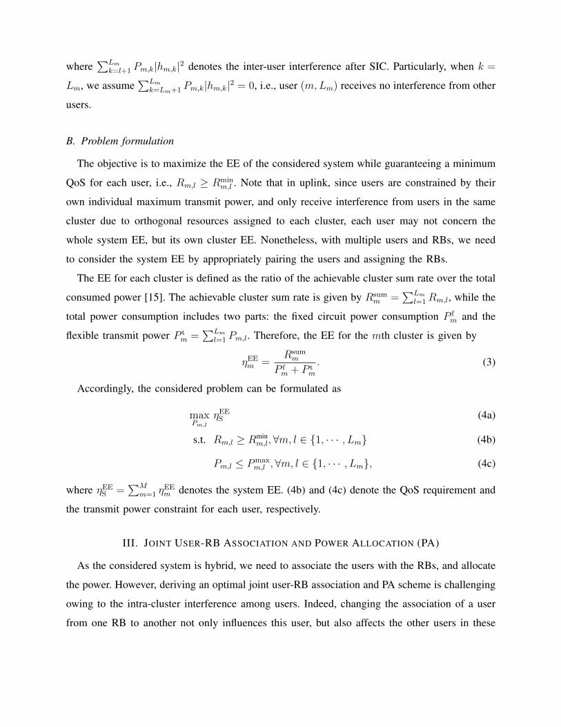
k=l+1 Pm,k|hm,k|2 denotes the inter-user interference after SIC. Particularly, when k =
Lm, we assume∑Lm
k=Lm+1 Pm,k|hm,k|2 = 0, i.e., user (m,Lm) receives no interference from other
users.
B. Problem formulation
The objective is to maximize the EE of the considered system while guaranteeing a minimum
QoS for each user, i.e., Rm,l ≥ Rminm,l . Note that in uplink, since users are constrained by their
own individual maximum transmit power, and only receive interference from users in the same
cluster due to orthogonal resources assigned to each cluster, each user may not concern the
whole system EE, but its own cluster EE. Nonetheless, with multiple users and RBs, we need
to consider the system EE by appropriately pairing the users and assigning the RBs.
The EE for each cluster is defined as the ratio of the achievable cluster sum rate over the total
consumed power [15]. The achievable cluster sum rate is given by Rsumm =
∑Lml=1Rm,l, while the
total power consumption includes two parts: the fixed circuit power consumption P fm and the
flexible transmit power P tm =
∑Lml=1 Pm,l. Therefore, the EE for the mth cluster is given by
ηEEm =
Rsumm
P fm + P t
m
. (3)
Accordingly, the considered problem can be formulated as
maxPm,l
ηEES (4a)
s.t. Rm,l ≥ Rminm,l,∀m, l ∈ {1, · · · , Lm} (4b)
Pm,l ≤ Pmaxm,l ,∀m, l ∈ {1, · · · , Lm}, (4c)
where ηEES =
∑Mm=1 η
EEm denotes the system EE. (4b) and (4c) denote the QoS requirement and
the transmit power constraint for each user, respectively.
III. JOINT USER-RB ASSOCIATION AND POWER ALLOCATION (PA)
As the considered system is hybrid, we need to associate the users with the RBs, and allocate
the power. However, deriving an optimal joint user-RB association and PA scheme is challenging
owing to the intra-cluster interference among users. Indeed, changing the association of a user
from one RB to another not only influences this user, but also affects the other users in these

RBs. Moreover, the objective function (4a) is non-convex, which makes it difficult to derive
conditions for optimality.
A. Proposed algorithm
To develop a low-complexity joint user-RB association and PA algorithm, we consider the
users and RBs as two sets of nodes in a bipartite graph. Then, the objective is to match the
users to the RBs and allocate power appropriately such that the EE can be maximized. First, we
define a matching as an assignment of RBs to users as follows.
Definition 1: Given two disjoint sets, U = {1, · · · , U} of the users, and M = {1, · · · ,M} of
the RBs, a many-to-one matching Φ is a mapping from the set U ∪M into the set of all subsets
of U ∪M such that for every u ∈ U and m ∈M:
1) Φ(u) ∈M;
2) Φ(m) ⊆ U ;
3) |Φ(u)| = 1;
4) |Φ(m)| = Lm;
5) m = Φ(u)⇔ u ∈ Φ(m),
where | · | returns the size of the matching. Conditions 1) and 3) state that each user is matched
with an RB, while conditions 2) and 4) imply that each RB is matched with Lm users.
Inspired by the many-to-one housing assignment problem [31], we introduce the notion of
swap matching into our many-to-one matching model, and propose a matching algorithm for the
joint user-RB association and PA problem [12]. A swapping operation means two users matched
with different RBs exchange their matches, while the matching for other users remains the
same. The PA is then updated for the two corresponding RBs. Note that how to allocate power
to obtain the EE for a given RB will be presented in the following sections, and we assume it is
known here. To ensure an improved EE performance, a swapping operation is approved and the
matching is updated only when the sum of the EEs for the two RBs involved increases after the
swap. Then, to maximize the EE of the considered system, the idea is to continue the swapping
operation until no swapping is further approved. Pseudocode for the proposed swapping-based
algorithm is given in Algorithm 1.
Note that in the initialization phase, the basic idea is to associate the user to the RB in which
it has a large channel gain. This leads to either a higher data rate for the user, or a lower transmit
power. Both yield a higher EE. Then, for the swap matching phase, iterations will continue until

no swapping operation can be approved in a new round.
B. Convergence and complexity
Theorem 1: The proposed joint user-RB association and PA algorithm converges after a finite
number of swapping operations.
Proof: After a number of swapping operations, the structure of matching changes as follows:
Φ0 → Φ1 → Φ2 → · · · , (5)
where Φ0 is the initial matching. For swapping operation l, the matching changes from Φl−1
to Φl. Denote the corresponding system EE as ηEES (l − 1) and ηEE
S (l). Therefore, we have
ηEES (l) > ηEE
S (l − 1), i.e., the system EE increases at each swapping operation. Moreover,
the system EE clearly has an upper bound due to the limited power and spectrum resources.
Consequently, the number of potential swapping operations is finite.
Given the convergence of the proposed algorithm, we discuss its computational complexity.
For the initial phase, it takes O(U2M) operations. In the swap matching phase, denote the
number of iterations to reach the final matching as I1.2 In each iteration, all possible swapping
combinations should be considered, which requires O(U2) operations. In each swapping attempt,
we need to conduct PA to calculate the EE before and after the swapping for the two related
clusters. Denote the computational complexity of the power allocation for calculating the EE as
O(X), which will be given in the following section. Then, the total complexity for the swap
matching phase is O(I1U2X). Adding this to the initial phase, we obtain the total complexity
as O(U2(I1X +M)).
IV. POWER ALLOCATION UNDER GIVEN USER-RB ASSOCIATION
In line 21 of Algorithm 1, we assume that the way of allocating power under a given user-RB
association is known. In this section, we present in detail how we conduct PA to maximize
the EE. Under a given user-RB association, we can conclude that maximizing the system EE is
equivalent to maximizing the EE for each cluster. This is because the system EE is the summation
2This number cannot be given in closed form, since we do not know for sure at which iteration the proposed algorithm reaches
the final matching. This is quite common in the design of most heuristic algorithms. To evaluate the convergence speed, we will
show the distribution of this number in the Simulation Results section.

Algorithm 1 Proposed joint user-RB association and PA algorithm.1: Step 1: Initialization phase
2: K ← d UMe, U ← U ;
3: for k = {1, · · · , K}
4: M ←M , Count← 1;
5: while (Count ≤M )
6: hm?,u? ← max{|hm,u|}|∀m∈M,∀u∈U
7: assign u? to RB m?;
8: U ← U\u?, M ← M\m?;
9: Count← Count + 1;
10: end while
11: end for
12: Step 2: Swap matching phase
13: Indicator = 1;
14: while (Indicator)
15: Indicator = 0;
16: for u ∈ {1, · · · , U},
17: for k ∈ {1, · · · , U}
18: if Φ(k) = Φ(u)
19: continue;
20: else
21: calculate and compare the EE before and after the swap using Algorithm 2;
22: if EE increases
23: update the matching, Indicator ← 1;
24: end if
25: end if
26: end for
27: end for
28: end while
over all cluster EEs, which are mutually independent as they are allocated with different RBs.
As a result, we can consider the EE maximization problem on each RB separately, and the mth
subproblem is given by
maxPm,l
ηEEm (6a)
s.t. Rm,l ≥ Rminm,l, l ∈ {1, · · · , Lm} (6b)
Pm,l ≤ Pmaxm,l , l ∈ {1, · · · , Lm}. (6c)
As the considered subproblems have the same form on different RBs, in the following sections,
we omit the RB index m for notational simplicity. Also, Lm is replaced by L while ηEEm is replaced
by ηEE.
A. Determine the feasibility
Owing to the minimum rate requirements and transmit power constraints, (6) may be infeasible,
i.e., there may not exist a PA solution to satisfy all the constraints. As a result, we need to find
the feasibility conditions first. Observe that the last user receives no interference from other users
due to SIC; we start with it and obtain
log2
(1 +
PL|hL|2
σ2
)≥ Rmin
L (7)
⇔PL ≥(2R
minL − 1)
|hL|2.
To satisfy the above requirement, we have
PmaxL ≥ (2R
minL − 1)
|hL|2. (8)
Assume that (8) is satisfied. Clearly, to reduce the interference from user L to other users, it
needs to use the minimum transmit power, i.e., PL = PminL = (2R
minL −1)|hL|2
. Now we consider the
(L− 1)th user. Likewise, we have
log2
(1 +
PL−1|hL−1|2
PL|hL|2 + σ2
)≥ Rmin
L−1
⇔ PL−1 ≥2R
minL (2R
minL−1 − 1)
|hL−1|2(9)
⇒ PmaxL−1 ≥
2RminL (2R
minL−1 − 1)
|hL−1|2.

Using the mathematical induction, we can easily extend it to all users, and obtain
Pmaxl ≥ Pmin
l =2∑Lk=l+1R
mink (2R
minl − 1)
|hl|2,∀l ∈ {1, · · · , L}, (10)
where Pminl is the minimum power required to satisfy the minimum rate requirement for the lth
user. Here we assume that∑L
k=L+1Rmink = 0. Once the above conditions between the minimum
rate requirements and the power constraints are satisfied, (6) is feasible.
B. Maximizing the EE when (6) is feasible
The objective function (6a) is of fractional form, which is non-convex and challenging to
handle. To tackle it, we first deal with the numerator, i.e., the sum rate, which can be re-written
as
Rsum =L∑l=1
log2
(1 +
Pl|hl|2∑Lk=l+1 Pk|hk|2 + σ2
)
= log2
(1 +
∑Ll=1 Pl|hl|2
σ2
). (11)
It is easy to see that the sum rate is a concave function with respect to (w.r.t.) the transmit
power for each user.
Now we consider the QoS constraints (6b). It is non- convex on its current form. However,
after some mathematical manipulations, it can be reformulated as
Pl|hl|2 ≥(
2Rminl − 1
)( L∑k=l+1
Pk|hk|2 + σ2
), (12)
which is a linear constraint, since it is just an affine mapping w.r.t., Pl, l ∈ {1, · · · , L}.
Accordingly, problem (6) can be re-written as
maxPl
log2
(1 +
∑Ll=1 Pl|hl|2σ2
)Pf +
∑Ll=1 Pl
(13a)
s.t. (12) (6c), l ∈ {1, · · · , L}. (13b)
For the objective function (13a), its numerator is a strictly concave function w.r.t., Pl, l ∈
{1, · · · , L}, while the denominator is an affine mapping over Pl, l ∈ {1, · · · , L}. Therefore, it
is a strictly pseudo-concave function [32, Proposition 6]. According to the property of strictly
pseudo-concave function, it can be optimally solved by applying the Dinkelbach’s algorithm
[32, Proposition 6]. The specific procedure is summarized in Algorithm 2. Denote the number
of iterations for Algorithm 2 to converge as I2. During each iteration, the proposed algorithm
needs to solve the following problem, i.e., line 4,
maxPl
log2
(1 +
∑Ll=1 Pl|hl|2
σ2
)− β(Pf +
L∑l=1
Pl) (14a)
s.t. (12) (6c), l ∈ {1, · · · , L}, (14b)
where β is known. Clearly, the above problem is concave, and can be solved using standard
algorithms, such as interior-point method. However, the standard approach does not exploit the
specific structure of (14), and is computationally intensive when (14) needs to be solved over and
over again. This is indeed the case here, since solving Algorithm 1 requires solving Algorithm
2 many times, i.e., line 21, and addressing Algorithm 2 also requires to solve (14) many times,
i.e., line 4. To relieve the computational burden, we propose a low-complexity optimal solution
for (14) as follows:
Denote F = log2
(1 +
∑Ll=1 Pl|hl|2σ2
)− β(Pf +
∑Ll=1 Pl). Then, for user l, we have ∂F
∂Pl=
|hl|2
ln 2(∑Lk=1 Pk|hk|2+σ2)
− β. Setting ∂F∂Pl
= 0, we obtain P 0l = 1
β ln 2−
∑k 6=l Pk|hk|2+σ2
|hl|2. If all other
power values, i.e., Pk, k 6= l are fixed, we can easily obtain the optimal solution for user l
by comparing P 0l with its minimum and maximum power constraints. Specifically, the optimal
power P ?l is given by
P ?l =
Pminl , if P 0
l < Pminl ,
Pmaxl , if P 0
l > Pmaxl ,
P 0l , otherwise.
(15)
On this basis, the proposed low-complexity algorithm goes as follows: we first allocate the
minimum required power to each user; then, we update the power for the users one by one
using (15); this update continues until convergence. Note that convergence is guaranteed since
F increases or remains unchanged after each update, and there exists an upper bound. Denote
the number of iterations for convergence as I3; then, its complexity is just O(I3). Thus, we have
X = I2I3, and O(U2(I1X +M)) = O(U2(I1I2I3 +M)). Moreover, the obtained local optimum
is also the global optimum since (14) is concave. The specific procedure is summarized in
Algorithm 3.
Remark: For any other SIC order, it can be easily proved that the objective function is the
same as (13a). Moreover, the minimum rate constraints can be turned into convex constraints

similar to (12). Therefore, Algorithms 2 and 3 can be directly used for EE maximization under
any other SIC order.
Algorithm 2 Proposed EE maximization PA algorithm.1: Initialize parameters.
2: Set ε > 0; β ← 0;F > ε;
3: while F > ε do
4: P ?l ← argmax log2
(1 +
∑Ll=1 Pl|hl|2σ2
)− β(Pf +
∑Ll=1 Pl); s.t. (12) (6c);
5: F ← log2
(1 +
∑Ll=1 P
?l |hl|
2
σ2
)− β(Pf +
∑Ll=1 P
?l );
6: β ←log2
(1+
∑Ll=1 P
?l |hl|
2
σ2
)Pf+
∑Ll=1 P
?l
;
7: end while
Although the proposed Algorithms 2 and 3 can be used to solve the considered EE maximiza-
tion problem, they do not shed much light into the behaviour of the system, since an iterated
algorithm is used. For example, how much power will be employed by the user with the highest
channel gain? To this end, several important properties are observed and listed in the sequel:
Lemma 1: Transferring power3 from a user with lower channel gain to a user with higher
channel gain leads to increased EE.
Proof: According to (13a), when the power transfer happens, the numerator increases owing
to the channel gain ordering. On the other hand, the sum transmit power remains unchanged,
and thus, the denominator remains unchanged. Therefore, the EE increases as well.
Theorem 2: If ∂ηEE
∂P1|Pmax
1 ,P−1≥ 0, user 1 should transmit at full power to maximize the EE,
where P−1 = P2, · · · , PL denotes a feasible PA solution for the other users.
Proof: First, when P1 = Pmax1 , the feasible region for the other users is maximized, since
the interference from user 1 is cancelled by SIC, and the minimum rate requirement of user 1 is
most likely to be satisfied. This means that if there exists a feasible region, P1 = Pmax1 is inside
it. Furthermore, since ∂ηEE
∂P1|Pmax
1 , P−1≥ 0, then P1 = Pmax
1 maximizes the EE, when P−1 remains
3Note that here transferring power means one user lowers his transmit power, while another user increases the same amount
of transmit power.

Algorithm 3 Proposed low-complexity algorithm for (14).1: Initialize parameters.
2: Set Pl ← Pminl , l ∈ {1, · · · , L};
3: while 1 do
4: Pold ← P ;
5: for l = {1, · · · , L};
6: P 0l = 1
β ln 2−∑k 6=i Pk|hk|2+σ2
hi|2 ;
7: if P 0l < Pmin
l
8: Pl ← Pminl ;
9: elseif P 0l > Pmax
l
10: Pl ← Pmaxl ;
11: else
12: Pl ← P 0l ;
13: end if
14: if |Pold − P | < 10−9
15: break;
16: end if
17: end for
18: end while
fixed [32, Proposition 5]. Next, we consider the case when power transfer happens between user
1 and other users. According to Lemma 1, transferring power from user 1 to other users leads
to a lower EE. Therefore, this will not happen. This completes the proof.
Theorem 3: If ∂ηEE
∂P1|Pmax
1 ,Pmin−1≤ 0, then Pl = Pmin
l , l 6= 1 and P1 = max(∂ηEE
∂P1|Pmin−1
= 0, Pmin1
),
where Pmin−1 = Pmin
2 , · · · , PminL denotes the minimum required power.
Proof: The derivative ∂ηEE
∂Plis given by
∂ηEE
∂Pl=
|hl|2
(σ2 +∑L
l=1 Pl|hl|2)(Pf +∑L
l=1 Pl) ln 2
−log2
(1 +
∑Ll=1 Pl|hl|2σ2
)(Pf +
∑Ll=1 Pl)
2. (16)
Clearly, the derivative ∂ηEE
∂Plis arranged following the same order of |hl|2, i.e., ∂ηEE
∂P1≥ · · · ≥

TABLE I: PA Solution for Two Users under Case I.
Phases Conditions Solutions
Phase I ∂ηEE∂P1|Pmax
1 ,Pmax2≥ ∂ηEE
∂P2|Pmax
1 ,Pmax2≥ 0 P1 ← Pmax
1 , P2 ← min
(Pmax2 ,
Pmax1 |h1|2
(2Rmin
1 −1)|h2|2− σ2
|h2|2
)Phase II
∂ηEE∂P1|Pmax
1 ,Pmax2≥ 0, ∂ηEE
∂P2|Pmax
1 ,Pmax2≤ 0 P1 ← Pmax
1 , set P ?2 ← ∂ηEE∂P2|Pmax
1= 0; if P ?2 ≤ Pmin
2 , then P2 ← Pmin2
∂ηEE∂P1|Pmax
1 ,Pmin2≥ 0
(Pmin2 = (2R
min2 −1)σ2
|h2|2
)else P2 ← min
(∂ηEE∂P2|Pmax
1= 0,
Pmax1 |h1|2
(2Rmin
1 −1)|h2|2− σ2
|h2|2
);
Phase III∂ηEE∂P1|Pmax
1 ,Pmax2≤ 0, ∂ηEE
∂P2|Pmax
1 ,Pmax2≤ 0, Same as Phase II
∂ηEE∂P1|Pmax
1 ,Pmin2≥ 0
(Pmin2 = (2R
min2 −1)σ2
|h2|2
)Phase IV ∂ηEE
∂P1|Pmax
1 ,Pmin2≤ 0, ∂ηEE
∂P2|Pmax
1 ,Pmin2≤ 0 P1 ← max
(∂ηEE∂P1|Pmin
2= 0, (2R
min1 −1)2R
min2 σ2
|h1|2
), P2 ← Pmin
2
TABLE II: PA Solution for Two Users under Case II.
Phases Conditions Solutions
Phase I ∂ηEE∂P1|Pmax
1 ,Pmax2≥ ∂ηEE
∂P2|Pmax
1 ,Pmax2≥ 0 P2 ← Pmax
2 , P1 ← min
(Pmax1 ,
Pmax2 |h2|2
(2Rmin
2 −1)|h1|2− σ2
|h1|2
)Phase II
∂ηEE∂P1|Pmax
1 ,Pmax2≥ 0, ∂ηEE
∂P2|Pmax
1 ,Pmax2≤ 0 if P
?1 ≤ Pmin
1 , then P1 ← Pmin1 , P2 ← (P
min1 − b)/k
if P?1 ∈ [P
min1 , Pmax
1 ], then P1 ← P?1, P2 ← P
?2
if P?1 ≥ Pmax
1 , then P1 ← Pmax1 , P2 ← ∂ηEE
∂P2|Pmax
1= 0
Phase III ∂ηEE∂P1|Pmax
1 ,Pmax2≤ 0, ∂ηEE
∂P2|Pmax
1 ,Pmax2≤ 0 same as Phase II
∂ηEE
∂Pl· · · ≥ ∂ηEE
∂PL. Since ∂ηEE
∂P1|Pmax
1 ,Pmin−1≤ 0, then ∂ηEE
∂Pl|Pmax
1 ,Pmin−1≤ 0,∀l ∈ {2, · · · , L}. Therefore,
all users should reduce their transmit power to increase the EE [32, Proposition 5]. On the other
hand, for all users except user 1, they can only reduce their power to the minimum required
power. So, we have Pl = Pminl , l 6= 1. Once all the other users’ powers are fixed, the EE is
maximized at the unique root of ∂ηEE
∂P1|Pmin−1
= 0 or the boundary point, i.e., Pmin1 . Combining
this, we can conclude that P1 = max(∂ηEE
∂P1|Pmin−1
= 0, Pmin1
).
Remark: Note that the condition for Theorem 2 holds when Pmaxl are quite small, while
that for Theorem 3 holds when Pmaxl are quite large. Thus, some good insights for these two
extreme cases have been derived. However, for the cases between these two extremes, it is quite
complicated to derive analytical results due to the coupling between the QoS requirements and
power constraints.

V. TWO USER CASE
Although it is challenging to derive the analytical solution for the general case of multiple
users, for the special case of two users, this is possible. Since the derivatives ∂ηEE
∂Plare arranged
as ∂ηEE
∂P1≥ · · · ≥ ∂ηEE
∂Pl· · · ≥ ∂ηEE
∂PL, for the two user case, there are only three cases to consider:
∂ηEE
∂P1≥ ∂ηEE
∂P2≥ 0, ∂ηEE
∂P1≥ 0 ≥ ∂ηEE
∂P2and 0 ≥ ∂ηEE
∂P1≥ ∂ηEE
∂P2. On the other hand, under different
SIC orders, the feasibility region is different, and thus, different PA solutions are required. The
two SIC orders need to be discussed separately. In the following, we first consider the case
for the SIC order which decodes user 1 first, and refer to it as Case I. Then, the other case is
considered, which is referred to as Case II.
A. Analytical solution when user 1 is decoded first
In this case, the PA solutions for the two users are listed in Table I.
Proof: Refer to Appendix I.
Remark: The bisection method can be used to find the root for the equation ∂ηEE
∂Pl= 0, with the
complexity of log2(Pmaxl /δ), where δ denotes the required precision. This is also the dominant
computation of obtaining the solution for the EE. According to Table I, when the system is
in Phases I, II or III, user 1 always transmits at full power. In Phase IV, user 2 transmits at
minimum power. Moreover, from Phase I to Phase IV, we can see how the users react when
the maximum allowable transmit power increases. In Phase I, the maximum allowable transmit
power is too small, and all the transmit power should be consumed not to violate the QoS
constraint. In Phases II and III, user 2 should only transmit with the power which ensures both
QoS and maximum EE.
B. Analytical solution when user 2 is decoded first
In this case, the problem can be formulated as
maxP1,P2
log2
(1 + P1|h1|2+P2|h2|2
σ2
)Pf + P1 + P2
(17a)
s.t. Pl ≤ Pmaxl ,m ∈ {1, 2}, (17b)
log2
(1 +
P2|h2|2
P1|h1|2 + σ2
)≥ Rmin
2 , (17c)
log2
(1 +
P1|h1|2
σ2
)≥ Rmin
1 , (17d)

where (17c) and (17d) represent the QoS requirements for user 2 and user 1, respectively. Note
that (17a) is the same as (13a) for two users. Indeed, for uplink NOMA, if there exists no QoS
constraints, the achievable sum rate under any SIC order is the same, and so is the EE. However,
with the QoS constraints, the feasibility region of the power may vary under different SIC orders,
and thus, leading to different sum rates and EEs.
The corresponding solution for the above problem is listed in Table II. Note that in this
table, we have Pmin
1 = (2Rmin1 −1)σ2
|h1|2 . Also, we replace P1 with P2 by considering that equality is
achieved at the minimum rate of user 2. Thus, we have P1 = P2|h2|2
(2Rmin2 −1)|h1|2
− σ2
|h1|2 = kP2 + b,
with k = |h2|2
(2Rmin2 −1)|h1|2
and b = − σ2
|h1|2 . Then, the multi-variable function of the EE becomes a
single variable function over P2, which is given by
f(P2) =log2
(1 + (kP2+b)|h1|2+P2|h2|2
σ2
)Pf + kP2 + P2 + b
. (18)
Correspondingly, the root of the derivative is denoted as P?
2 ← f′(P2) = 0. The corresponding
value for P1 is P?
1 = kP?
2 + b.
Proof: Refer to Appendix II.
Remark: It can be seen that changing the SIC order leads to different PA results. Under Case
II, even for Phases I and II, user 1 may not transmit at full power. For Phase I, instead, user
2 transmits at full power. Also, it is quite difficult to judge which decoding order is better,
since this depends on the transmit power constraint and the QoS requirement. If both constraints
are the same for both users, under Phase I, it is clear that Case I always outperforms Case II.
However, even in this case, except from Phase I, it is still difficult to compare them analytically.
TABLE III: Simulation Parameters.
Parameters Value
Number of users per cluster L = 2, 3
Number of RBs M = 1, 4, 8
Minimum rate requirement Rmin = 1.5 [bit/s/Hz]Fixed Transmit power per user Pf = 0 [dBm]
Channel bandwidth per RB 180 [KHz]Noise power spectral density −174 [dBm/Hz]
Path-loss model 128 + 35 log10(d), d in kilometerSmall scale fading CN (0, 1)
-15 -10 -5 0 5 10 15
Maximum transmit power (dBm)
0
500
1000
1500
2000
2500
3000
3500
4000
EE
(bi
t/J/H
z)
NOMA: 2 usersNOMA: 3 usersOMA: 2 usersOMA: 3 users
MaxEE
MaxSE
(a)
-15 -10 -5 0 5 10 15
Maximum transmit power (dBm)
-20
-15
-10
-5
0
5
10
15
Tra
nsm
it po
wer
(dB
m)
P1
P2
P3
Pmax
(b)
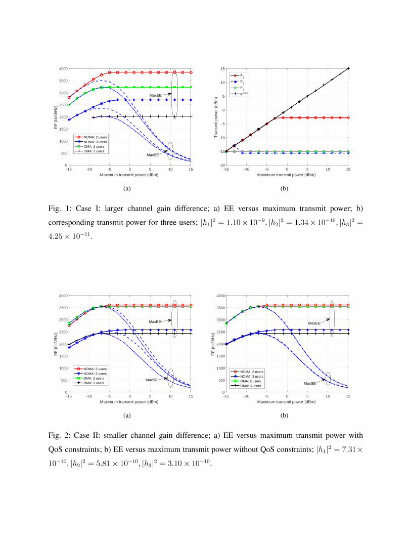
Fig. 1: Case I: larger channel gain difference; a) EE versus maximum transmit power; b)
corresponding transmit power for three users; |h1|2 = 1.10× 10⁻⁹, |h2|2 = 1.34× 10⁻¹⁰, |h3|2 =
4.25× 10⁻¹¹.
-15 -10 -5 0 5 10 15
Maximum transmit power (dBm)
0
500
1000
1500
2000
2500
3000
3500
4000
EE
(bi
t/J/H
z)
NOMA: 2 usersNOMA: 3 usersOMA: 2 usersOMA: 3 users
MaxSE
MaxEE
(a)
-15 -10 -5 0 5 10 15
Maximum transmit power (dBm)
0
500
1000
1500
2000
2500
3000
3500
4000
EE
(bi
t/J/H
z)
NOMA: 2 usersNOMA: 3 usersOMA: 2 usersOMA: 3 users
MaxEE
MaxSE
(b)
Fig. 2: Case II: smaller channel gain difference; a) EE versus maximum transmit power with
QoS constraints; b) EE versus maximum transmit power without QoS constraints; |h1|2 = 7.31×
10−10, |h2|2 = 5.81× 10⁻¹⁰, |h3|2 = 3.10× 10⁻¹⁰.

VI. SIMULATION RESULTS
In this section, simulations are conducted to verify the developed results. The default simulation
parameters are listed in Table III. Note that in simulations, we assign the same minimum rate
requirements and maximum transmit power constraints to all users.
A. Single cluster
Results for two cases with different channel gain difference between the users are shown
in Figs. 1 and 2. In addition, as a baseline algorithm, OMA with equal degrees of freedom
is presented. The results are also obtained by running the proposed Algorithm 2 with the rate
expressions adjusted according to the OMA protocol. Moreover, we also present the results when
the objective is to maximize the SE of the system, which is denoted as “MaxSE”. In contrast,
the EE maximizing results are denoted as “MaxEE”. From Figs. 1(a) and 2(a), we can see
that the EE first increases with the maximum transmit power for both “MaxEE” and “MaxSE”.
Then, after a certain threshold, “MaxEE” saturates, while “MaxSE” continues to decrease. This
illustrates the importance of applying an energy-efficient PA algorithm, especially under high
maximum transmit power.
Specifically, Fig. 1 shows the case with larger channel gain difference among the users. In this
case, NOMA achieves much higher EE than OMA for both two and three users, respectively.
Moreover, for both NOMA and OMA, the two user case is much better than the three user
case. Fig. 1(b) shows how the three users allocate their power as the maximum transmit power
increases. For user 1, under low maximum transmit power, full power is consumed, which agrees
with Theorem 2. Under high maximum transmit power, its power no longer increases with the
maximum transmit power, but saturates. This coincides with Theorem 3. Moreover, for users 2
and 3, they are transmitting using the minimum required power, as expected based on Theorem
3.
Fig. 2 shows the case of smaller channel gain difference. In this case, for both OMA and
NOMA, the two user case is better than the three user case. However, under low maximum
transmit power, OMA is better than NOMA. This is because the interference introduced by
NOMA leads to a smaller feasibility region. Take two user case for example, under low maximum
transmit power, OMA is transmitting at full power for both users. However, if Pmax1 |h1|2
(2Rmin1 −1)|h2|2
−σ2
|h2|2 < Pmax2 , user 2 in NOMA cannot transmit at full power to ensure the QoS of user 1.
This is quite different from the downlink case, in which the BS controls the PA for all users,

-15 -10 -5 0 5 10 15
Maximum transmit power (dBm)
-5
0
5
10
15
20
Der
ivat
ive
valu
e
×106
DP1
DP2
DP3
(a)
-15 -10 -5 0 5 10 15
Maximum transmit power (dBm)
-30
-25
-20
-15
-10
-5
0
5
10
15
Tra
nsm
it po
wer
(dB
m)
Pmax
Case I: P1
Case I: P1
'
Case I: P2
Case I: P2
'
Case II: P1
Case II: P1
'
Case II: P2
Case II: P2
'
(b)
Fig. 4: Comparison between two SIC orders; a) Partial derivative values; b) PA; |h1|2 = 1.10×
10−9, |h2|2 = 1.34× 10⁻¹⁰.
-15 -10 -5 0 5 10 15
Maximum transmit power (dBm)
1500
2000
2500
3000
3500
4000
EE
(bi
t/J/H
z)
Case ICase II
Fig. 3: Comparison of the EE between the two SIC orders; |h1|2 = 1.10× 10⁻⁹, |h2|2 = 1.34×
10−10.
and can distribute power among them. In uplink, each user is constrained by its own maximum
transmit power. Since user 1’s power cannot be increased over its maximum transmit power,
the allowable power for user 2 cannot be increased either. Consequently, NOMA achieves lower
EE than OMA. In Fig. 2(b), we show the case when there is no QoS constraints. As expected,
NOMA is always better than OMA, even though the gain is quite minor for the two user case.
Comparing this with Fig. 1, it implies that user pairing should be conducted such that the users’

channel gain should be distinct. Moreover, it is worth mentioning that NOMA still outperforms
OMA under high maximum transmit power.
In Figs. 3 and 4, we compare the performance between the two SIC orders. According
to Fig. 3, Case I achieves much higher EE than Case II. Fig. 4(a) shows how the partial
derivative values vary with the maximum transmit power, where DP1, DP2 and DP3 denote∂ηEE
∂P1|Pmax
1 ,Pmax2
, ∂ηEE
∂P2|Pmax
1 ,Pmax2
and ∂ηEE
∂P2|Pmax
1 ,Pmin2
, respectively. It can be seen that as the maxi-
mum transmit power increases, Case I moves from Phase I to Phase IV, while Case II moves from
Phase I to Phase III. In Fig. 4(b), we plot P1 and P2 obtained by Algorithm 2 (without prime)
and the proposed analytical solution (with prime). Obviously, the same results are obtained by
both methods, which demonstrates the correctness of the analytical solution.4 Particularly, under
low maximum transmit power, the system is in Phase I, user 1 in Case I and user 2 in Case II
transmit at full power.
B. Multiple clusters
In this subsection, multiple clusters are considered. We compare the proposed solution, denoted
as HMA-prop, with two OMA-based algorithms, i.e., OMA-swap and OMA-MWM, and three
HMA-based algorithms, i.e., HMA-DC [14], HMA-MWM and HMA-rand. OMA-swap follows
the same procedure as HMA-prop, but with the rate expressions adjusted according to the
OMA protocol. In OMA-MWM, we update the PA and user-RB association alternately until
convergence. More exactly, under a given PA, it is clear that the EE maximization is equivalent
to the sum rate maximization. According to the OMA protocol, the achievable rate of user (m, l)
is ROm,l = 1
Lmlog2
(1 +
LmPm,l|hm,l|2σ2
), which depends only on the allocated RB. Consider the
users and RBs as the two set of nodes in a bipartite graph, and the corresponding rates ROm,l
as the weights. Then, the matching that maximizes the sum weight also maximizes the sum
rate, and further the EE. This matching can be obtained efficiently using standard maximum
weight matching (MWM) algorithms, such as the Hungarian algorithm [33]. Under a given user-
RB association, the PA can be solved using Algorithm 2, with the rate expressions adjusted
according to the OMA protocol. Note that convergence is guaranteed since the EE increases or
remains unchanged after each update, and there exists an upper bound.
4As we use the log value on the y-axis, it may seem that for Case II, there exists a difference between these two algorithms.
Indeed, the difference is smaller than 10−5, and it exists simply because the root can only be approximated using the bisection
method.

-15 -10 -5 0 5 10 15
Maximum transmit power (dBm)
1.2
1.3
1.4
1.5
1.6
1.7
1.8
1.9E
E (
bit/J
/Hz)
104
HMA-propHMA-MWMHMA-DC [14]OMA-swapOMA-MWMHMA-rand
(a)
-15 -10 -5 0 5 10 15
Maximum transmit power (dBm)
1.5
1.6
1.7
1.8
1.9
2
2.1
2.2
2.3
EE
(bi
t/J/H
z)
104
HMA-propHMA-MWMHMA-DC [14]OMA-swapOMA-MWMHMA-rand
(b)
Fig. 5: Comparison of average EE when U = 12 and M = 4; a) smaller channel gain difference;
b) larger channel gain difference.
-15 -10 -5 0 5 10 15
Maximum transmit power (dBm)
2.6
2.8
3
3.2
3.4
3.6
3.8
4
EE
(bi
t/J/H
z)
104
HMA-propHMA-MWMHMA-DC [14]OMA-swapOMA-MWMHMA-rand
(a)
-15 -10 -5 0 5 10 15
Maximum transmit power (dBm)
2.8
3
3.2
3.4
3.6
3.8
4
4.2
4.4
4.6
4.8
EE
(bi
t/J/H
z)
104
HMA-propHMA-MWMHMA-DC [14]OMA-swapOMA-MWMHMA-rand
(b)
Fig. 6: Comparison of average EE when U = 24 and M = 8; a) smaller channel gain difference;
b) larger channel gain difference.
HMA-DC is the scheme proposed in [14], in which each user sends its matching request to
its most preferred RB based on the channel gain. However, the preferred RB only accepts the
users that lead to the maximum EE. The rejected users will move to the next preferred RB and
this process continues until all users are matched to an RB. For HMA-MWM, we cannot apply
it the same way as for OMA-MWM, since MWM for HMA cannot be performed due to the

intra-cluster interference. Instead, we simply consider the weights to be the channel gains. Then,
we conduct the MWM between the users and the RBs to achieve the maximum sum channel
gains. In HMA-rand, the users are allocated to the RBs randomly.
The following results are averaged over 103 random trials, and for each trial, we generate the
users’ locations following a uniform distribution. We first present the result when there are 12
users accessing 4 RBs. We consider two cases with different channel gain differences. Fig. 5(a)
shows the result when all users lie within a radius of 150 m. In Fig. 5(b), the users are equally
divided into three circles, with radii of 50, 100 and 150 m, respectively. Therefore, Fig. 5(a) is
the case with smaller channel gain difference. It is clear that HMA-prop is the best, followed by
HMA-MWM, HMA-DC, HMA-rand OMA-MWM and OMA-swap. This validates the superiority
of the proposed scheme over other HMA- and OMA-based algorithms. In Fig. 5(b), it can be
seen that HMA-prop is still the best, followed by HMA-MWM and HMA-DC. However, in this
case, OMA-swap outperforms OMA-MWM, and HMA-rand is the worst. Quite surprisingly, by
comparing Figs. 5(a) and 5(b), we can observe that a larger channel gain difference does not
necessarily lead to a larger gain of HMA over OMA. This does not contradict the conclusion
in the single cluster, where we claim that a large channel gain difference among users yields a
larger gain of HMA over OMA. This is because the user-RB association results in HMA and
OMA can be quite different, and the former conclusion holds when the user-RB association
remains the same for both schemes.
Figure 6 shows the result when we double the number of users and RBs, i.e., now there are
24 users accessing 8 RBs. By comparing Figs. 5 and 6, it is clear that the corresponding EE
values in Fig. 6 are more than twice those in Fig. 5, except for HMA-rand. This implies that a
multiplexing gain is obtained by having more RBs.
Figure 7 plots the cumulative distribution function (CDF) of the number of swapping operation
required to reach convergence for the above two scenarios. It can be seen that the number of
swapping operations grows with that of RBs. However, less than 60 swapping operations are
needed even for the scenario when U = 24 and M = 8, which is quite small. In addition, for
Algorithm 3, simulation results show that exactly 6 iterations are required for it to converge
when there are 3 users sharing an RB.

0 10 20 30 40 50 60
Number of swap operations
0
0.1
0.2
0.3
0.4
0.5
0.6
0.7
0.8
0.9
1
CD
F o
f the
num
ber
of s
wap
ope
ratio
nsU=12, M=4U=24, M=8
Fig. 7: CDF of the number of swap operations for convergence.
VII. CONCLUSION
In this paper, we have studied the energy-efficient resource allocation for HMA uplink with
QoS requirements for each user. Based on swap matching in many-to-one bipartite graph, we
have proposed a joint user-RB association and power allocation scheme, which is guaranteed to
converge. Under a given user-RB association, we have shown that the system EE maximization
equals cluster EE maximization. Then, we have derived the feasibility conditions, and proposed
to solve the EE maximization using Dinkelbach’s algorithm. Moreover, to further relieve the
computational burden, a low-complexity optimal algorithm has been proposed for solving the
convex optimization subproblem inside the Dinkelbach’s algorithm. For the two user case,
analytical solutions have further been derived for the two SIC orders. Simulations have been
performed, which verify the developed analytical solutions. Moreover, the results for a single
cluster show that under low maximum transmit power, OMA can be better than HMA for uplink,
due to the smaller feasibility region for HMA caused by the QoS requirements. On the other
hand, under high maximum transmit power, HMA still outperforms OMA. Results under multiple
clusters fully validate the superiority of the proposed scheme over other HMA- and OMA-based
algorithms. Furthermore, a multiplexing gain can be observed when employing more RBs.
In this work, we have considered the situation in which each user can access a single RB.
The extension to multiple RBs is interesting for future work.

APPENDIX A
PROOF OF TABLE I
In Phases I, II and III, as it satisfies the condition for Theorem 2, we can conclude that
P1 = Pmax1 . As for Phase IV, it is exactly the condition for Theorem 3, and thus, the conclusion
holds. Then, we only need to prove the PA for user 2 in Phases I, II and III.
Let us first consider Phase I. For the differentiable strictly pseudo-concave function, since∂ηEE
∂P1|Pmax
1 ,Pmax2≥ ∂ηEE
∂P2|Pmax
1 ,Pmax2≥ 0, we can conclude that ∂ηEE
∂P1≥ ∂ηEE
∂P2≥ 0 for any value of P1
and P2. Thus, increasing the transmit power for each user leads to an larger EE. However, for
user 2, increasing P2 also causes more interference to user 1. To ensure the QoS requirement of
user 1, the maximum power can be used by user 2 is given by Pmax1 |h1|2
(2Rmin1 −1)|h2|2
− σ2
|h2|2 . Combining
this with the transmit power constraint, we have P2 = min
(Pmax
2 ,Pmax1 |h1|2
(2Rmin1 −1)|h2|2
− σ2
|h2|2
).
Next, let us focus on Phases II and III. Without considering the QoS constraint, P2 is obtained
when ∂ηEE
∂P2|Pmax
1= 0. Denote it as P ?
2 , satisfying P ?2 < Pmax
2 . On the other hand, due to the
minimum rate requirements for user 1 and user 2, P2 has a lower bound Pmin2 , and an upper bound
Pmax1 |h1|2
(2Rmin1 −1)|h2|2
− σ2
|h2|2 . If P ?2 ≤ Pmin
2 , P2 = Pmin2 . Otherwise, P2 = min
(P ?
2 ,Pmax1 |h1|2
(2Rmin1 −1)|h2|2
− σ2
|h2|2
).
APPENDIX B
PROOF OF TABLE II
In Phase I, due to the change of SIC order, user 2 should transmit at full power. As for user 1, it
should not violate the QoS requirement of user 2, and thus, P1 <Pmax2 |h2|2
(2Rmin2 −1)|h1|2
− σ2
|h1|2 . Combining
it with the maximum power constraint, we have P1 = min
(Pmax
1 ,Pmax2 |h2|2
(2Rmin2 −1)|h1|2
− σ2
|h1|2
).
In Phases II and III, we first assume that P1 is constrained by the QoS of user 2. Then, we
turn the multi-variable function into a single variable function. Accordingly, the solution for this
is the root of the derivative. Denote this as P?
2. Correspondingly, P?
1 = kP?
2 + b. On the other
hand, user 1 needs to satisfy its own QoS, and thus, we obtain Pmin
1 . If P?
1 < Pmin
1 , P1 = Pmin
1 ,
and P2 = (Pmin
1 − b)/k. If P2 < (Pmin
1 − b)/k, it cannot satisfy its own QoS. If P2 exceeds
this, EE decreases, since P2 > P?
2, and P1 > P?
1. When P?
1 lies in (Pmin
1 , Pmax1 ), if P
?
2 ≤ Pmax2 ,
P1 = P?
1, P2 = P?
2 is clearly the solution. As for the case P?
2 > Pmax2 , this cannot hold. This
is because we can transfer power from user 2 to user 1, and increase the EE. Therefore, P?
2
cannot be the root of (18). When P?
1 > Pmax1 , P1 = Pmax
1 . Denote the root of ∂ηEE
∂P2|Pmax
1as P r
2 .
Since ∂ηEE
∂P2|Pmax
1 ,Pmax2≤ 0, P r
2 ≤ Pmax2 . In addition, we can obtain P r
2 ≥ (Pmax1 − b)/k, owing

to ∂ηEE
∂P2|Pmax
1 ,(Pmax1 −b)/k ≥ ∂ηEE
∂P2|P ?1,P ?2 = 0. Therefore, the QoS of user 2 can be satisfied when
P1 = Pmax1 and P2 = P r
2 . In sum, we can conclude that P2 = P r2 .
REFERENCES
[1] M. Zeng, A. Yadav, O. A. Dobre, and H. V. Poor, “Energy-efficient power allocation for uplink NOMA,” in Proc IEEE
Globecom, Abu Dhabi, UAE, Dec. 2018, pp. 1–6.
[2] S. M. R. Islam, M. Zeng, O. A. Dobre, and K. Kwak, “Resource allocation for downlink NOMA systems: Key techniques
and open issues,” IEEE Wireless Commun. Mag., vol. 25, no. 2, pp. 40–47, Apr. 2018.
[3] Z. Ding, Y. Liu, J. Choi, Q. Sun, M. Elkashlan, and H. V. Poor, “Application of non-orthogonal multiple access in LTE
and 5G networks,” IEEE Commun. Mag., vol. 55, no. 2, pp. 185–191, Feb. 2017.
[4] S. M. R. Islam, M. Zeng, and O. A. Dobre, “NOMA in 5G systems: Exciting possibilities for enhancing spectral efficiency,”
IEEE 5G Tech. Focus, vol. 1, no. 2, May 2017. [Online]. Available: 307 http://5g.ieee.org/tech-focus.
[5] L. Dai, B. Wang, Y. Yuan, S. Han, C. L. I, and Z. Wang, “Non-orthogonal multiple access for 5G: Solutions, challenges,
opportunities, and future research trends,” IEEE Commun. Mag., vol. 53, no. 9, pp. 74–81, Sep. 2015.
[6] S. M. R. Islam, et al., “Power-domain non-orthogonal multiple access (NOMA) in 5G systems: Potentials and challenges,”
IEEE Commun. Surv. Tuts., vol. 19, no. 2, pp. 721–742, Second quarter 2017.
[7] F. Zhou, Y. Wu, R. Q. Hu, Y. Wang, and K. K. Wong, “Energy-efficient NOMA enabled heterogeneous cloud radio access
networks,” IEEE Network, vol. 32, no. 2, pp. 152–160, Mar. 2018.
[8] M. Zeng, G. I. Tsiropoulos, O. A. Dobre, and M. H. Ahmed, “Power allocation for cognitive radio networks employing
non-orthogonal multiple access,” in Proc. IEEE Global Commun. Conf., Washington DC, USA, Dec. 2016.
[9] Z. Ding, Z. Yang, P. Fan, and H. V. Poor, “On the performance of non-orthogonal multiple access in 5G systems with
randomly deployed users,” IEEE Signal Process. Lett., vol. 21, no. 12, pp. 1501–1505, Dec. 2014.
[10] M. Zeng, A. Yadav, O. A. Dobre, G. I. Tsiropoulos, and H. V. Poor, “On the sum rate of MIMO-NOMA and MIMO-OMA
systems,” IEEE Wireless Commun. Lett., vol. 6, no. 4, pp. 534–537, Aug. 2017.
[11] ——, “Capacity comparison between MIMO-NOMA and MIMO-OMA with multiple users in a cluster,” IEEE J. Select.
Areas Commun., vol. 35, no. 10, pp. 2413–2424, Oct. 2017.
[12] B. Di, L. Song, and Y. Li, “Sub-channel assignment, power allocation, and user scheduling for non-orthogonal multiple
access networks,” IEEE Trans. Wireless Commun., vol. 15, no. 11, pp. 7686–7698, Nov. 2016.
[13] M. Zeng, A. Yadav, O. A. Dobre, and H. V. Poor, “A fair individual rate comparison between MIMO-NOMA and MIMO-
OMA,” in Proc IEEE Globecom Wkshps, Singapore, Dec 2017, pp. 1–5.
[14] F. Fang, H. Zhang, J. Cheng, and V. C. M. Leung, “Energy-efficient resource allocation for downlink non-orthogonal
multiple access network,” IEEE Trans. Commun., vol. 64, no. 9, pp. 3722–3732, Sep. 2016.
[15] Y. Zhang, H. M. Wang, T. X. Zheng, and Q. Yang, “Energy-efficient transmission design in non-orthogonal multiple
access,” IEEE Trans. Veh. Technol., vol. 66, no. 3, pp. 2852–2857, Mar. 2017.
[16] W. M. Hao et al., “Energy-efficient power allocation in millimeter wave massive MIMO with non-orthogonal multiple
access,” IEEE Wireless Commun. Lett., vol. PP, no. 99, pp. 1–1, Jun. 2017.
[17] M. Zeng, A. Yadav, O. A. Dobre, and H. V. Poor, “Energy-efficient power allocation for MIMO-NOMA with multiple
users in a cluster,” IEEE Access, vol. 6, pp. 5170–5181, Feb. 2018.
[18] W. Hao, Z. Chu, F. Zhou, S. Yang, G. Sun, and K. Wong, “Green communication for NOMA-based CRAN,” IEEE Internet
of Things J., pp. 1–1, 2018.

[19] T. Lv, Y. Ma, J. Zeng, and P. T. Mathiopoulos, “Millimeter-wave NOMA transmission in cellular M2M communications
for internet of things,” IEEE Internet of Things J., vol. 5, no. 3, pp. 1989–2000, Jun. 2018.
[20] Y. Endo, Y. Kishiyama, and K. Higuchi, “Uplink non-orthogonal access with MMSE-SIC in the presence of inter-cell
interference,” in Proc IEEE ISWCS, Aug. 2012, pp. 261–265.
[21] X. Chen, A. Benjebbour, A. Li, and A. Harada, “Multi-user proportional fair scheduling for uplink non-orthogonal multiple
access (NOMA),” in IEEE VTC, May. 2014, pp. 1–5.
[22] W. Liu, X. Hou, and L. Chen, “Enhanced uplink non-orthogonal multiple access for 5G and beyond systems,” Front.
Inform. Technol. Electron. Eng., vol. 19, no. 3, pp. 340–356, Mar. 2018.
[23] Y. Liang, X. Li, J. Zhang, and Z. Ding, “Non-orthogonal random access for 5G networks,” IEEE Trans. Wireless Commun.,
vol. 16, no. 7, pp. 4817–4831, July 2017.
[24] M. Shirvanimoghaddam, M. Condoluci, M. Dohler, and S. J. Johnson, “On the fundamental limits of random non-orthogonal
multiple access in cellular massive IoT,” IEEE J. Select. Areas Commun., vol. 35, no. 10, pp. 2238–2252, Oct. 2017.
[25] L. Zhu et. al, “Joint power control and beamforming for uplink non-orthogonal multiple access in 5G millimeter-wave
communications.” arXiv preprint arXiv:1711.06162, 2017.
[26] M. S. Ali, H. Tabassum, and E. Hossain, “Dynamic user clustering and power allocation for uplink and downlink non-
orthogonal multiple access (noma) systems,” IEEE Access, vol. 4, pp. 6325–6343, Aug. 2016.
[27] D. Zhai and J. Du, “Spectrum efficient resource management for multi-carrier-based NOMA networks: A graph-based
method,” IEEE Wireless Commun. Lett., vol. 7, no. 3, pp. 388–391, Jun. 2018.
[28] T. Lv, Z. Lin, P. Huang, and J. Zeng, “Optimization of the energy-efficient relay-based massive IoT network,” IEEE Internet
of Things J., vol. 5, no. 4, pp. 3043–3058, Aug. 2018.
[29] Z. Yang, W. Xu, H. Xu, J. Shi, and M. Chen, “Energy efficient non-orthogonal multiple access for machine-to-machine
communications,” IEEE Commun. Lett., vol. 21, no. 4, pp. 817–820, Apr. 2017.
[30] M. Zeng, W. Hao, O. A. Dobre, and V. Poor, “Energy-efficient power allocation in uplink mmwave massive MIMO with
NOMA,” IEEE Trans. Veh. Technol., pp. 1–1, 2019.
[31] E. Bodine-Baron, C. Lee, A. Chong, B. Hassibi, and A. Wierman, “Peer effects and stability in matching markets,” in
Proc. 4th Symp. Algorithmic Game Theory (SAGT), Amalfi, Italy, Oct. 2011, pp. 117–129.
[32] A. Zappone, P. Lin, and E. Jorswieck, “Energy efficiency in secure multi-antenna systems,” IEEE Trans. Signal Process.,
submitted for publication. [Online]. Available: http://arxiv.org/abs/1505.02385.
[33] H. W. Kuhn, “The hungarian method for the assignment problem,” Naval Research Logistics (NRL), vol. 1-2, pp. 83–97,
1955.


![arXiv:1503.02445v3 [cs.CV] 1 Apr 2015muhammad.uzair@research.uwa.edu.au, ffaisal.shafait, ajmal.miang@uwa.edu.au bernard.ghanem@kaust.edu.sa Abstract Efficient and accurate joint](https://img.dokumen.tips/doc/110x75/5f61c3616eec2d687f30c17a/arxiv150302445v3-cscv-1-apr-2015-researchuwaeduau-ffaisalshafait-ajmalmianguwaeduau.jpg)