Energy Consumption Analysis of WirelessNetworks using Stochastic Deployment Models

Vinay Suryaprakash*, Andre Fonseca dos Santos**, Albrecht Fehske*, Gerhard P. Fettweis**Vodafone Chair Mobile Communications Systems, TU Dresden, Germany(vinay.suryaprakash,albrecht.fehske,gerhard.fettweis)@ifn.et.tu-dresden.de

**Bell Labs, Alcatel-Lucent, Stuttgart-Germany(A.Santos@alcatel-lucent.com)

Abstract—This paper aims to discuss the influence of ad-justable base station (BS) power parameters, such as powerconsumed during active mode and sleep modes, on the overallenergy consumption of a network and highlight potential energysavings that can be achieved by the introduction of sleep modes.A BS density that can satisfy the demands of a given userdensity – defined by a daily traffic profile – can be found usingthe relationship between spatially averaged rate, user density,and BS density established here. The underlying framework forthis relationship assumes users and BSs to be independentlymarked point processes in R2. A power model that is an affinefunction of the BS density is used to determine the overall energyconsumption of the network at full load, and these values arecompared to those that incorporate sleep modes to utilize theminimum number of BSs that satiate the demands of a userdensity that varies during the course of the day. The relationshipestablished between spatially averaged rate, user density, and BSdensity forms the main result of this paper, based on which itcan be inferred that the introduction of sleep modes results insubstantial energy savings when the load is seldom full.

I. INTRODUCTION

A perpetual expansion of cellular networks is requiredto meet an increasingly exacting user demand, which lendsitself to estimating its environmental impact. It’s been shownthat the carbon footprint of cellular networks is estimatedto almost triple by 2020 [1]. A key to stunting the carbonfootprint of future cellular networks is minimizing the overallenergy consumption of a network. With this in mind, twobasic paths have been pursued in the literature thus far:hardware improvements, and the introduction of sleep modes.Improving hardware is the most palpable attempt at savingenergy in a network. When macro BSs are considered, thepower amplifier is the biggest source of energy inefficiency.Therefore, considerable effort has been put into findingmethods for reducing the energy consumption of poweramplifiers (e.g. [2], [3]).

Although improvements in hardware are essential forthe overall success of efforts toward making the networkmore energy efficient, energy management strategies thatprudently exploit fluctuations in the load (of a network) forenergy savings have to be designed to ensure that the energyconsumed at any given point in time is minimized. Onesuch energy management strategy is the introduction of sleep

modes. Sleep modes, in this context, are defined as modeswhere a sizable fraction of the hardware in a BS is switchedoff, and it should not be confused with micro sleep modeswhere only a small fraction of the hardware is switched offduring a short interval (as seen in [2], [3]) – on the order ofa few micro seconds. Several propositions for sleep modeshave been made in recent literature (e.g. [4]–[6]). Practicalsolutions that allow BSs to be switched off while maintainingcoverage are being proposed in consortia like GreenTouch1.One such idea consists of separating the data and signalingnetworks [7], where the signaling network ensures coveragewhile BSs catering to data requirements are placed in sleepmode (when not being utilized). Strategies that demonstratethese gains, in terms of achievable energy savings, are usuallyvalidated using lengthy Monte Carlo simulations. In thispaper, a theoretic framework based on stochastic geometryis proposed for such an evaluation. To grasp the effects ofrandomness in deployments, BS locations are considered tobe homogeneous Poisson point processes. The use of randomdeployments also allows conclusions to be drawn about theefficacy of a particular energy conservation strategy, or thelack there of, by providing information about the averagevalues of a metric of interest for an area under consideration,i.e. the values provided are averaged over all possible celltopologies. The validity of using Poisson process based BSdeployments to mimic real world deployments is shown in[8]. This is then used to predict energy savings that can beachieved in a network with macro BSs.

This paper considers the downlink of a wireless network andprovides a general expression that relates spatially averagedrate with user and BS densities for a given path loss exponent(Subsection II-A). This can be considered an extensionof the general expression derived in [8]. Details of thedifferences between the expressions derived are highlightedin the upcoming section (Section II). This expression formsa foundation for the analysis of the energy consumption of anetwork with a fixed user demand and a known user densitywhich varies according to a traffic profile (given in [9]).A linear power model, whose details are elucidated in the

1http://greentouch.org

following, is used to find the average energy consumption ofa network through the day. The power model and its utilityare given in Section III. The energy saving potential of sleepmodes are discussed in Subsection III-B, based on which,conclusions and future work are delineated in Section IV.

II. DOWNLINK SYSTEM MODEL

A downlink interference limited system model is consideredwhere single antenna BSs are arranged according to somehomogeneous Poisson point process Φb , with intensity λb(BS density) in the Euclidean plane. The users are consideredto be located according to an independent stationary Poissonpoint process Φu, with intensity λu (user density). Since thereare usually a larger number of users than BSs, it is assumedthat they are both non-zero and λu > λb. The noise poweris assumed to be zero (i.e. W = 0), hence the model isinterference limited. The Euclidean plane is assumed to betessellated around the BS process and the Voronoi cell isdefined as:

CXb ={y ∈ R2 : SIRy ≥ T

}={y ∈ R2 : L (y, xi) ≥ T (IΦb (y))

}where Xb = {xi} is the set of BS locations, T is the threshold,and SIRy is the Signal-to-Interference Ratio at y. L(y, xi) isreceived power at point y, and IΦb (y) is the interference at y.The received power and the interference are defined as

L(y, xi) =Ph

l (|y − xi|); IΦb (y) =

∑xj ,j 6=i

L (y, xj) ,

where P is the transmit power, h is a fading parameterdefined as an exponential random variable with mean 1. Thisimplies that the product Ph at any point y (i.e. the powerthat is received at a given point without taking the pathlossinto consideration) can be represented by an exponentialrandom variable of mean P−1. Lastly, l (|y − xi|) is the omni-directional path loss function which can be represented asl (r) = (Ar)

β , for some A > 0 and the path loss exponentβ > 2, where r is the distance between the point y andthe BS at xi. The interference received at a point y is alsodependent on the number of users connected to a BS, an aspectwhich has not been included in [8]. The general expressionderived in this paper includes this aforementioned aspect, andcan therefore be considered an extension of their findings.The average number of users connected to a given BS hasbeen shown to be E (N) = λu/λb in [10], where λu is theuser density and λb is the BS density. Incorporating this fact,results in the product Ph that is exponentially distributed withmean (λuP/λb)

−1. These parameters are used to derive theprobability of coverage (i.e. probability that a point y ∈ R2 iscovered by its nearest BS, xi ∈ Xb) and the spatially averagedrate of the system for the energy consumption analysis.

A. Probability of Coverage and Spatially Averaged Rate

Theorem 1. The probability of coverage for a path lossexponent β > 2 and a threshold t is:

pc (λb, λu, t) =β − 2

(β − 2) +2λut2F1

(1, β−2

β ;2− 2β ; −tλuλb

)λb

(1)

From which the spatially averaged rate for a path lossexponent, β = 4 can be shown to be:

RΦb(λb, λu) =

∫ ∞0

2y[1 + y tan−1 (y)

] [y2 + λu

λb

]dy (2)

Further simplification to establish a complete analytic rela-tionship gives eqn.(3).

Proof: The average rate can be written as

RΦb(λb, λu) = Eo [log(1 + SIRo) > γ] ,

where Eo is the Palm expectation, γ is the threshold, andSIRo is the Signal-to-Interference Ratio at the origin. Note:The origin is always assumed to be at the point that isbeing considered. The spatially average rate RΦb(λb, λu) thenbecomes

Eo [log(1 + SIRo) > γ] = Eo [SIRo > eγ − 1] .

Using the Refined Campbell Theorem [11],

RΦb(λb, λu) =

∫ ∞γ=0

∫r>0

Po (SIRo > eγ − 1) Λb (dr) .

Here, Po is the Palm distribution of SIRo and Λb is theintensity measure of the BS Poisson process. By the Theoremof Slivnyak [11], the spatially average rate is given by

RΦb(λb, λu) =

∫ ∞0

∫ ∞0

2πλbr exp(−πλbr2

)P (SIRo > eγ − 1) drdγ.

From [10], the probability of coverage or the probability thata point y ∈ R2 is covered by its nearest transmitter can bedefined as

pc (λb, λu, t) =

∫ ∞0

2πλbr exp(−πλbr2

)P (SIRo > t) dr

=

∫ ∞0

2πλbr exp(−πλbr2

)LIΦb

(µtrβ

)dr,

where LIΦb(µtrβ

)is the Laplace transform of the interference

and µ is the fading mean, and it’s assumed that the constant‘A’ in the omni-directional path loss function is equal to 1for the rest of this proof. The above equation implies that thespatially averaged rate can then be written as

RΦb(λb, λu) =

∫ ∞0

pc (λb, λu, (eγ − 1)) dγ. (4)

The probability of coverage can be written as

pc (λb, λu, t) =

∫ ∞0

2πλbr exp(−πλbr2

)×

exp

(−2πλb

∫u>r

u(1− LP

(µtuβ/rβ

))du

)dr,

RΦb(λb, λu) =2

9

81π2

(λuλb

)5/2

+ 18(λuλb

)log

(9π2

(λuλb

)3

4

)− 36 · 3

√2 · 6√

3 · π5/3(λuλb

)2

+ 8 · (2)2/3 · (3)

5/6 · 3√π

9π2(λuλb

)3

+ 4

(3)

where LP(µtuβ/rβ

)is the Laplace transform of the power

received at a point y. This implies

pc (λb, λu, t) =

∫ ∞0

2πλbr exp(−πλbr2

)×

exp

−2πλb

∫ ∞r

u

1 + λbλu

(uβ

trβ

)dudr.

Therefore, if

λb (β − 2) + 2tλuRe

[2F1

(1,β − 2

β; 2− 2

β;−tλuλb

)]> 0

and

2F1

(1,β − 2

β; 2− 2

β;−tλuλb

)∈ R,

the probability a point y ∈ R2 is covered by its nearest basestation when there are λu

λbusers connected to any given base

station is

pc (λb, λu, t) =β − 2

(β − 2) +2λut2F1

(1, β−2

β ;2− 2β ; −tλuλb

)λb

,

where 2F1 (a, b; c; z) is the Gaussian hypergeometric function.Since the values of λu, λb are positive, the threshold t ≥ 0, andβ > 2, it’s easy to show that the above conditions are satisfied.

Substituting the result obtained above in equation (4)gives the spatially averaged rate, RΦb(λb, λu)

=

∫ ∞0

β − 2

(β − 2) +2λu(eγ−1)2F1

(1, β−2

β ;2− 2β ;

−(eγ−1)λuλb

)λb

dγ.

Substituting (eγ−1)λuλb

= tan2 (z), we get the average rate tobe

=

∫ π/2

0

2 (β − 2) tan(z) sec2(z)[(β − 2) + 2 tan2(z)2F1

(1, β−2

β ; 2− 2β ;− tan2(z)

)]×1[

tan2(z) + λuλb

]dz.Assuming β = 4, changing the limits of integration usingtan(z) = y, and then applying Euler’s transformation to thehypergeometric results in

RΦb(λb, λu) =

∫ ∞0

2y[1 + y tan−1 (y)

] [y2 + λu

λb

]dy.Using the series expansion of the inverse trigonometric func-tion and integrating over the limits gives RΦb(λb, λu) to beequal to equation (3).

B. Analysis of Results

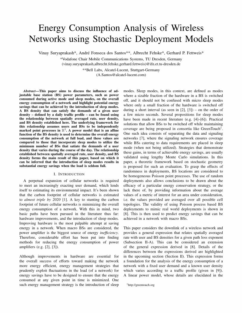
The theorem provides the spatially averaged rate that can beachieved over a normalized area in bps/Hz. The plot obtainedusing the theorem above has been shown to concur withthe plot obtained for the system model under considerationby Monte Carlo simulations in figures Fig. 1a and Fig. 1b,respectively. These plots indicate the variation in the spatiallyaveraged rate with increasing user and BS densities.

There are, however, a few obvious differences – the reasonsfor which are explained in the remainder of this section. The

05

1015

20

0

5

100

0.5

1

1.5

2

2.5

User DensityBS Density

Avg

. Rat

e

(a) Theoretic Rate Vs. λu Vs. λb

05

1015

20

0

5

10

150

1

2

3

4

User Density (λu)

BS Density(λb)

Avg

. Rat

e

(b) Simulated Rate Vs. λu Vs. λb

Fig. 1. Comparison of theoretic results with simulations

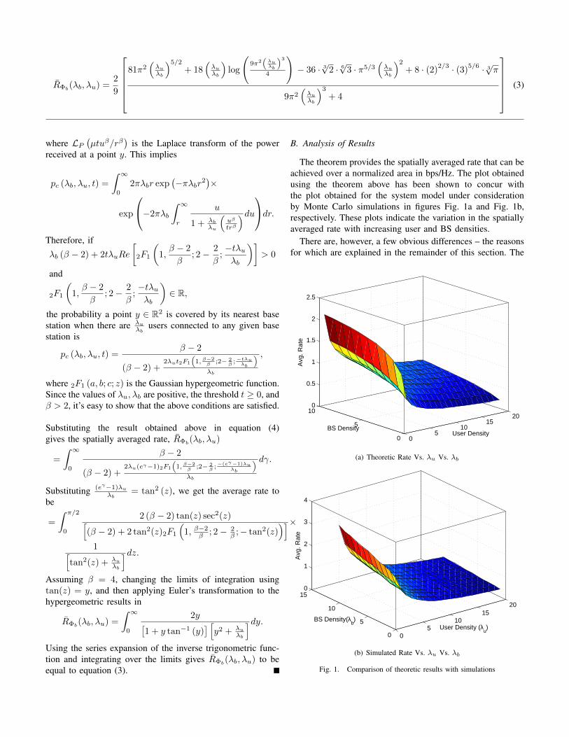
peak average theoretic rate is slightly lower than the peakaverage rate obtained by simulations. This is due to the factthat the theoretic case averages over a far greater number ofrates (that are close to zero), by considering different cellsizes which are obtained by integrating over thresholds from0 to ∞, whereas during simulations the number of iterationsthat determine varying cell sizes (though large) are finite.Another factor responsible for this discrepancy is the area ofobservation: it is considered to be all of R2 in the theoreticcase, whereas, the simulations consider a large (finite) areafor generating the points of the Poisson process and observerates over smaller windows to effectively mimic the theoreticcase. Smoothness of the curves is another aspect that differs.The simulated curve is less smooth due to the inability toevaluate an expectation precisely with simulations. Fig. 2.shows a plot of variation in the theoretic spatially averagedrate (equation (3)) versus the ratio of user density and BSdensity (i.e. λu/λb).

0 5 10 15 200

0.2

0.4

0.6

0.8

1

1.2

Ratio of User to BS Density (λu/λ

b)

Spa

tially

Ave

rage

d R

ate

(bps

/Hz)

Fig. 2. Spatially averaged rate Vs.(λuλb

)The figure (Fig. 2.) is utilized in the analysis of the energy

consumption of a network using the power model describedin the section below.

III. ENERGY CONSUMPTION MODEL

The power consumption model of a BS, as in [9], is assumedto be:

Pc =

{∆pPTx + P0 if the BS is activePS if the BS is in sleep mode (5)

where PTx is the transmit power, P0 is the power consumedby the BS at the lowest possible output power, and ∆p is theslope of the load dependent power consumption. The metricof interest, however, is the power density which is “powerconsumed per square kilometer” (W/km2). It follows that thepower density (without sleep modes) can be defined as:

DP = λbPc = λb (∆pPTx + P0) (6)

Note that equation (6) assumes that all BSs use the sametransmit power. Considering a homogeneous Poisson pointprocess to represent BSs implies that all BSs in the networkare of the same type and we consider them to be macroBSs. The values considered for calculations shown below aretaken from [9]. The framework to calculate the average energyconsumption of the network per square kilometer over a periodof 24 hours is as follows:

1) For a given user demand D Mbps, a daily traffic/loadprofile η(t), and maximum rate density per unit area (UMbps/km2); the user density (users/km2) at a given timeof day can be found by:

λu =Uη(t)

D(7)

2) The average rate that is provided by the system (R) isalways assumed to meet or exceed user demands, i.e.R ≥ D. The spatially averaged rate RΦb(λb, λu) derivedabove has the units of bps/Hz and for a given bandwidthB, it can be given as:

RΦb(λb, λu) =R

B(8)

3) The user to BS density ratio that can satisfy the averagerate obtained using equation (8) is found using Fig. 2.

4) The number of BSs required to provide the average ratein equation (8), is found by dividing the user densityfound in equation (7) by the ratio of user to BS densities(i.e. the value of λu/λb from the x-axis of Fig. 2).

5) The BS density found in the step above is then usedin equation (6) to obtain the power density required tosatisfy a particular user demand over the entire area.

6) Inferences about the overall energy consumption of thenetwork and the effectiveness of sleep modes (whendeployed) are drawn from comparison of power densitiesobtained under different load constraints.

0%

20%

40%

60%

80%

100%

120%

0h 1h 2h 3h 4h 5h 6h 7h 8h 9h 10h 11h 12h 13h 14h 15h 16h 17h 18h 19h 20h 21h 22h 23h

η(t)

Hours of the day

Daily Traffic Profile

Data Traffic

Fig. 3. Daily traffic/ load profile

The values considered for our energy consumption analysisare as follows:

1) User demand, D = 2 Mbps; Maximum rate densityper unit area for a dense urban deployment, U = 120Mbps/km2; and the load profile η(t) is shown in Fig. 3.

2) The average rate provided by the system, R is consideredto be 2 Mbps unless specified as being otherwise.

3) The effective bandwidth B = 6.39 MHz, which isobtained by considering a 10 MHz LTE system ( 600sub-carriers, frequency spaced at 15 KHz, and a controloverhead of 29%).

4) Slope of the load dependent power consumption, ∆p

= 5.32; Transmit power PTx = 20 W; Fixed powerconsumed, P0 = 118.7 W. The values of sleep modepower PS are assumed to vary depending on the typeof sleep mode considered. For ex: PS = 0.5 W for deepsleep mode. Note: Since there are no practical valuesavailable, we use 0.5 W which is the typical powerconsumption of standby mode in Wi-Fi transmitters.

Note: The values of parameters in step (4) above are obtainedfrom [9].

A. Analyzing the energy consumption of the network

Consider a scenario without sleep modes and the followingobservations can be made:

0,00

20,00

40,00

60,00

80,00

100,00

120,00

140,00

160,00

180,00

200,00

0h 1h 2h 3h 4h 5h 6h 7h 8h 9h 10h 11h 12h 13h 14h 15h 16h 17h 18h 19h 20h 21h 22h 23h

W/s

q.k

m

Hours of the day

Daily Power Density Fluctuation

Power Density Fluctuation for 2Mbps

Fig. 4. Daily fluctuations in power density

Fig. 4 shows that the plot of power density through the dayfollows the daily traffic profile (Fig. 3) very closely, if a linearpower model (like the one described above) is used.

Fig. 5 shows the variation in the number of BSs requiredper square kilometer when the average rate R provided by thenetwork increases from 2 Mbps to 5 Mbps in unit increments,while all other values remain unchanged. It’s observed thatevery (individual) curve in the plot of the BS density throughthe day (Fig. 5) also varies according to the daily traffic profile(Fig. 3). Another aspect worth examining is the amount ofadditional power that needs to be provided to increase theaverage rate (R) available at any given point by 1 Mbps. Fig.6 validates our expectations in this regard, and indicates thatthe amount of power required to increase the average rate (R)of the network by 1 Mbps increases nonlinearly. For example:

1

2

3

4

5

6

7

0h 1h 2h 3h 4h 5h 6h 7h 8h 9h 10h 11h 12h 13h 14h 15h 16h 17h 18h 19h 20h 21h 22h 23h

BS/

sq.k

m

Hours of the day

BS's per square Km

BS/sq.Km for 2Mbps BS/sq.Km for 3 Mbps BS/sq.Km for 4 Mbps BS/sq.Km for 5Mbps

Fig. 5. BS density per square kilometer

the figure indicates that trying to increase the average rate (R)provided by the network from 6 Mbps to 7 Mbps consumesmore than 4 times the power that is required to increase theaverage rate from 2 Mbps to 3 Mbps when all other parametersare kept unchanged. This is due to the non-linearity in therelationship between BS density and the spatially averagedrate as seen in eqn.(3).

0,00

1,00

2,00

3,00

4,00

5,00

6,00

7,00

8,00

3 - 4 Mbps 4 -5 Mbps 5 - 6 Mbps 6 -7 Mbps 7 - 8 MbpsNu

mb

er

of

tim

es

the

ad

dit

ion

al p

ow

er

req

uir

ed

Unit increase in Average Rate provided

Additional Power Density Requirement

Multiplication factor when compared to an increase from 2 Mbps to 3 Mbps

Fig. 6. Additional power density requirement

B. Energy consumption analysis using sleep modesIn practice, BS deployments are usually designed to be able

to satisfy user demands when they are operating under full load(i.e. η(t) =100%). To reflect this scenario, the maximum BSdensity and the power density which correspond to a full loadscenario are found using the procedure expounded above. Thenumber of BSs that can be turned off per square kilometerare found by subtracting the BS density required to satisfythe load during a specified hour of the day from the densityrequired to meet the demands at full load. The power saveddue to the introduction of sleep modes is given by:

Power Saved = DPmax −DP − (λbmax − λb)PS (9)

where DPmax is the power density at 100% load, λbmax is theBS density required at 100% load, DP is the power densityat a given load, and λb is the BS density at the same load.

0,00

20,00

40,00

60,00

80,00

100,00

120,00

140,00

160,00

180,00

0h 1h 2h 3h 4h 5h 6h 7h 8h 9h 10h11h12h13h14h15h16h17h18h19h20h21h22h23h

W/s

q.k

m

Hours of the day

Power Saved

Power Saved in W/sq.km with P_s = 0.5 W

Power Saved in W/sq.km with P_s = 50 W

Power Saved in W/sq.km with P_s = 93 W

Fig. 7. Power saved through the day

Fig. 7 shows the potential power saving that can beachieved by restricting the number of BSs in active mode tothat which satiates the demands of a given load and turningthe other BSs off. A deep sleep mode power value has beenassigned for sleep mode power (i.e. PS = 0.5 W) in the figure(Fig. 7). The values of PS are varied from 0.5 W, which isassumed to be typical of a deep sleep mode where the BSsare turned off for a long period of time, to 93 W (which isillustrative of micro sleep modes where a small fraction ofthe hardware is turned off [9]). From the figure, it is observedthat as PS increases, the energy saved at any given hour ofthe day decreases. This indicates that energy savings can stillbe achieved as long as PS is less than P0. It also validatesthe linear relationship between PS and power saved that isapparent from equation (9).

For the traffic profile considered in Fig. 3, it is noted thatapproximately 40% of the power density consumed daily (anaverage of about 72 W/km2 can be saved per day) when deepsleep modes are used and approximately 23% of the powerdensity consumed daily (an average of about 42 W/km2 perday) can be saved when a sleep mode power of 93W is used,for satisfying a user demand of 2 Mbps. This indicates thatdeep sleep modes can, on average, almost double the powersaved per square kilometer per day.

IV. CONCLUSION

For an interference limited downlink system model, analyticexpressions for the probability of coverage and the averagerate have been found. The expression relates spatially averagedrate with user and BS densities, and has been used to providevaluable insights about the energy consumption of a network.For a linear power model, it can be concluded that the numberof BSs required per square kilometer to meet a given user

demand and the power density (in W/km2) follow variationsin traffic density very closely. Another valuable insight, is thefact that the additional power density required to increase theaverage rate provided by the network by 1 Mbps increasesnon-linearly as the initial (preexisting) average rate providedincreases. The analytic expressions also allow examinationof the utility of sleep modes and help confirm that sleepmodes can, indeed, provide significant power savings when thenetwork operates in conditions of less than full load. It alsoconfirms the intuition that, for any traffic profile η(t), deepsleep modes help save more power than other sleep modes.For the traffic profile considered here, deep sleep modes almostdouble the average power saved when compared with using thesleep mode power of micro sleep modes (i.e. PS = 93W). Theenergy consumption analysis and an affirmation of benefits ofsleep modes provided by this paper, though insightful, are farfrom presenting a holistic solution to the problem considered.Questions such as the effect of noise on the system, or theenergy consumption of a network with different BS types(micro and macro BSs), and comparison of theoretic results(shown here) with simulations and real world models areleft unanswered. The effects of utilizing more complicatedpower models, within the framework described here, are alsounknown. An effort to answer some of the questions posedabove forms the basis for future work of the authors.

ACKNOWLEDGMENT

This work is a part of the GreenTouch consortium.

REFERENCES

[1] A. Fehske, J. Malmodin, G. Biczok, and G. Fettweis, “The GlobalCarbon Footprint of Mobile Communications - The Ecological andEconomic Perspective,” IEEE Communications Magazine, vol. 49, no. 8,Aug. 2011.

[2] A. Ambrosy, O. Blume, H. Klessig, and W. Wajda, Potential of In-tegrated Hardware and Resource Management Solutions for WirelessBase Stations. accepted for Workshop W-GREEN in conjunction withPIMRC, 2011.

[3] P. Frenger, P. Moberg, J. Malmodin, Y. Jading, and I. Godor, ReducingEnergy Consumption in LTE with Cell DTX. Vehicular TechnologyConference (VTC Spring), 2011.

[4] K. Dufkov, M. Bjelica, B. Moon, L. Kencl, and J. Le Boudec, EnergySavings for Cellular Network with Evaluation of Impact on Data TrafficPerformance. European Wireless Communications, 2010.

[5] J. Lorincz, A. Capone, and D. Begusic, Optimized network managementfor energy savings of wireless access networks. Computer Networks,2011.

[6] L. Chiaraviglio, D. Ciullo, M. Meo, and M. Ajmone Marsan, Energy-Efficient Management of UMTS Access Networks. 21st InternationalTeletraffic Congress, Paris, France, 2009.

[7] A. Capone, A. F. dos Santos, I. Filippini, and B. Gloss, “Looking beyondgreen cellular networks,” in Wireless On-demand Network Systems andServices (WONS), 2012 9th Annual Conference on, jan. 2012, pp. 127–130.

[8] J. G. Andrews, F. Baccelli, and R. K. Ganti, “A tractable approach tocoverage and rate in cellular networks,” CoRR, vol. abs/1009.0516, 2010.

[9] G. Auer, V. Giannini, I. Godor, P. Skillermark, M. Olsson, M. A. Imran,D. Sabella, M. Gonzales, C. Desset, and O. Blume, “Cellular energyefficiency evaluation framework,” Green Wireless Communications andNetworks Workshop 2 with VTC, 2011.

[10] F. Baccelli and B. Blaszczyszyn, “Stochastic Geometry and WirelessNetworks Volume 1: THEORY,” Foundations and Trends in Networking,vol. 3, pp. 249–449, 2009.

[11] R. Schneider and W. Weil, Stochastic and Integral Geometry. Springer-Verlag, 2008.