Embed Size (px)
Citation preview

Syed Jobairul Alam
ENERGY AND SPECTRAL EFFICIENCY TRADEOFF IN WIRELESS
COMMUNICATION
Faculty of Information Technology and Communication
Sciences Master of Science Thesis
October 2019

i
ABSTRACT
SYED JOBAIRUL ALAM: ENERGY AND SPECTRAL EFFICIENCY TRADEOFF IN WIRELESS COMMUNICATION Master of Science Thesis Tampere University Master’s Degree Program in Electrical Engineering October 2019
In the wireless communication world, a significant number of new user equipments is connecting to the network each and every day, and day after day this amount is increasing with no known bounds. Diverse quality of service (QoS) along with better system throughput are the crying needs at present. With the advancement in the field of massive multiple-input multiple-output (MMIMO) and Internet-of-things (IoT), the QoS is provided smoothly with the limited spectrum by the wireless operator. Hundreds of antenna elements in the digital arrays are set up at the base station in order to provide the smooth coverage and the best throughput within these spectra. However, implementing hundreds of antenna elements with associated a huge number of RF chains for digital beamforming consumes too much energy. Energy efficiency optimization has become a requirement at the present stage of wireless infrastructure. Due to the conflicting nature between the energy efficiency and the spectral efficiency, it is hard to make a balance. This thesis investigates how to achieve a good tradeoff between the energy and the spectral efficiency with maximum throughput outcomes from MMIMO, with the help of existing topologies and a futuristic perspective. Although the signal noise power is less in massive MIMO than the conventional cellular system, it still needs to be decreased and at the same time, the average channel gain per user equipment must be increased. Fixed power requirement for control signaling and load-independent power of backhaul infrastructure must be cut at least by a factor two as well as the power amplifier efficiency has to increase by 10% than LTE networks. The minimum mean square error (MMSE) estimator can be a possible solution in terms of the energy and the spectral efficiency despite having computational complexity which can be solved with the aid of Moore’s law and it is proposed by the non-profit research organization IMEC, which has developed an online web tool for observing and predicting contemporary as well as futuristic cellular base station’s power consumption. It supports various types of base stations with a wide range of operating conditions. The multicell minimum mean square error (M-MMSE) scheme can perform better than other existing schemes and showcase satisfactory tradeoff with frequency reuse factor higher than 2, where regularized zero-forcing (RZF) and maximum ratio (MR) combining fall down their capabilities for performing. With the precipitous rising of IoT, the Narrowband Internet-of-things (NB-IoT) may play an efficient supportive role if we can collaborate it with MMIMO. With its low power, wide area topologies combining with MMIMO technologies can show better tradeoffs. Due to its narrow bandwidth, the signal noise power would be less compared to the existent wideband topologies, and the average channel gain of active user equipment would be higher too. Hence it will give a great impact in terms of the tradeoff between energy and the spectral efficiency which is addressed in this thesis.
Keywords: Spectral efficiency, energy efficiency, throughput, massive MIMO, NB-IoT
The originality of this thesis has been checked using the Turnitin Originality Check service.

PREFACE
All praise goes to the supreme creator ALLAH, who has given me enough courage and
patience to complete my master’s thesis. The process wasn’t easy, neither the roadmap.
There were lots of ups and downs, enormous unsuccessful attempts, countless
awakened nights, but finally, HE enlightened me with the right and successful
approaches to come to an end.
I want to thank cordially to my thesis supervisor, Associate Professor, Dr. Elena Simona
Lohan for mentoring me, motivating me and giving me this beautiful as well as updated
topic. Her supervision and time asking for feedback help me to complete my thesis.
Secondly, I want to thank my Co-supervisor, Dr. Jukka Talvitie for giving me his precious
time and guiding me. Thank you so much from the core of my heart and thanks once
again to keep faith in me and my capabilities.
Special thanks go to Tampere University for giving me the chance to peruse my higher
education. Really thankful to the entire faculty, my friends and my family.
This is a milestone achievement in the journey of my life. Though it is not the end, it will
always encourage me in every step in my life.
Tampere, 18 October 2019
Syed Jobairul Alam

CONTENTS
1. INTRODUCTION .................................................................................................. 1
1.1 Thesis Objectives ................................................................................. 2
1.2 Author’s Contributions .......................................................................... 2
1.3 Thesis Structure ................................................................................... 3
2. CONCEPTS OF D2I AND D2D ............................................................................. 4
2.1 D2I (Device-to-Infrastructure) Concept ................................................. 4
2.2 D2D (Device-to-Device) Concept ......................................................... 5
2.3 IoT (Internet-of-Things) ........................................................................ 6
2.4 Massive MIMO ..................................................................................... 7
2.5 Pilot Contamination .............................................................................. 9
2.6 Channel Estimation ............................................................................ 10 2.6.1 Minimum Mean Square Error (MMSE) ........................................ 10
2.6.2 Element–Wise Minimum Mean Square Error (EW-MMSE) .......... 10
2.6.3 Least-Square (LS) Channel Estimator ......................................... 11
2.7 Precoding And Combining Schemes .................................................. 11 2.7.1 Multicell-Minimum Mean Square Error (M-MMSE) ...................... 11
2.7.2 Singlecell-Minimum Mean Square Error (S-MMSE) .................... 11
2.7.3 Regularized Zero-Forcing (RZF) ................................................. 12
2.7.4 Zero-Forcing (ZF) ........................................................................ 12
2.7.5 Maximum Ratio (MR) Combining ................................................ 12
2.8 Unimodal Function ............................................................................. 13
3. DEFINITIONS OF SPECTRAL AND ENERGY EFFICIENCY ............................. 14
3.1 Spectral Efficiency Definitions ............................................................ 14 3.1.1 Link Spectral Efficiency ............................................................... 15
3.1.2 Area Spectral Efficiency or System Spectral Efficiency ............... 15
3.2 Energy Efficiency ............................................................................... 15
4. SIMULATIONS TO ENHANCE SPECTRAL & ENERGY EFFICIENCY ............... 20
4.1 Achievable Uplink Spectral Efficiency ................................................ 20 4.1.1 Impact of Spatial Channel Correlation ......................................... 24
4.1.2 Impact of Pilot Contamination and Coherent Interference ........... 26
4.1.3 SE with Other Channel Estimation Schemes than MMSE ........... 28
4.2 Energy Efficiency ............................................................................... 30 4.2.1 Hotspot Tier ................................................................................ 30
4.2.2 Asymptotic Analysis of Transmit Power ...................................... 32
5. SIMULATIONS AND RESULTS .......................................................................... 34
6. CONCLUSION .................................................................................................... 54
REFERENCES....................................................................................................... 56

LIST OF FIGURES
Figure 1. Basic D2I (Device-to-Infrastructure) inventory model. ................................... 5 Figure 2. Basic D2D (Device-to-Device) inventory model ............................................. 6 Figure 3. Advantages of MMIMO over existent technology. ......................................... 8 Figure 4. Illustration of basic massive MIMO network setup ......................................... 9 Figure 5. Power consumed in percentage by different components of BS
coverage tier ........................................................................................ 16 Figure 6. Basic block diagram of coverage BS’s power-consuming hardware
element ................................................................................................ 17 Figure 7. Average UL sum SE for five different combining schemes as a function
of the number of BS antennas, M ......................................................... 22 Figure 8. Average UL sum SE for five different combining schemes as a function
of the number of BS antennas, M ......................................................... 23 Figure 9. Average UL sum SE using the Gaussian local scattering channel model
as a function of varying ASD ................................................................ 25 Figure 10. Average UL power of the desired signal with coherent interference
and non-coherent interference ............................................................. 27 Figure 11. Average UL sum SE of M-MMSE, RZF, and MR combining by using
MMSE, EW-MMSE, and LS estimator .................................................. 29 Figure 12. Average DL sum SE with normalized MR precoding as a function of
the number of antennas, M .................................................................. 33 Figure 13. Energy Efficiency curve with respect to the number of transmitters ........... 35 Figure 14. G(K, NTX) as a function of UEs with respect to the number of antennas .... 36 Figure 15. Linear dependence between maximum EE and SE for different values
of BS’s fixed power, PFIX ...................................................................... 37 Figure 16. EE and SE relationship for different values of BS’s antennas, M ............... 38 Figure 17. EE versus SE relation for different σ2/ β values. ....................................... 39 Figure 18. EE versus SE relation for wide range of antennas, M ................................ 41 Figure 19. EE as a function of SE for different of M/K ratios. ...................................... 42 Figure 20. EE as a function of average throughput per cell for L = 16 ........................ 44 Figure 21. EE as a function of average throughput per cell for L = 32 ........................ 45 Figure 22. EE as a function of average throughput per cell for L = 32 ........................ 46 Figure 23. EE as a function of average throughput per cell for L = 64 ........................ 46 Figure 24. EE as a function of average throughput per cell for the NB-IoT with
MMIMO system .................................................................................... 47 Figure 25. EE as a function of throughput for value set 2 and number of BS, L =
32......................................................................................................... 48 Figure 26. EE as a function of throughput for value set 2 and number of BS, L =
64......................................................................................................... 49 Figure 27. EE as a function of throughput for value set 2 and number of BS, L =
128 ....................................................................................................... 49 Figure 28. Maximal EE as a function of M/K for the M-MMSE combining scheme ...... 51 Figure 29. Maximal EE as a function of M/K for the RZF combining scheme. ............ 51 Figure 30. Maximal EE as a function of M/K for MR combining scheme. .................... 52

LIST OF TABLES
Table 1. Comparison of different LPWAN technologies for IoT operation ..................... 7 Table 2. System parameters regarding Massive MIMO and NB-IoT ........................... 21 Table 3. Average UL sum SE [bits/s/Hz/cell] for different pilot reuse factors ............... 24 Table 4. Average DL throughput over 20 MHz channels per cell ................................ 31 Table 5. BS’s CP model based on the combining and precoding schemes. ................ 43
LIST OF SYMBOLS AND ABBREVIATIONS
ADC Analog-to-Digital Converter ASD Angular Standard Deviation ATP Area Transmit Power AWGN Additive White Gaussian Noise BS Base Station CDF Cumulative distribution function CP Circuit Power CSI Channel State Information D2D Device-to-Device D2I Device-to-Infrastructure DAC Digital-to-Analog Converter DL Downlink EC-GSM-IoT Extended Coverage Global System for Mobile Internet-of-Things EE Energy Efficiency eNB eNode B ETP Effective Transmit Power EW-MMSE Element-Wise MMSE FEC Forward Error Control FDD Frequency-Division Duplex GSM Global System for Mobile Communications HSPA+ Evolved High Speed Packet Access I/Q In-Phase/Quadrature LoRA Long-Range LO Local Oscillator LoS Line-of-Sight LPWAN Low Power Wide Area Network LS Least-Squares LTE Long Term Evolution LTE-M Long Term Evolution for Machine MAC Medium Access Control MIMO Multiple-Input Multiple-Output MMIMO Massive Multiple-Input Multiple-Output M-MMSE Multicell Minimum-Mean Square Error MMSE Minimum-Mean Square Error MSE Mean-Squared Error MOO Multi-objective Optimization MR Maximum Ratio MRC Maximum Ratio Combining MRT Maximum Ratio Transmission NB-IoT Narrowband Internet-of-Things NLoS Non-Line-of-Sight OFDM Orthogonal Frequency-Division Multiplexing PA Power Amplifier PC Power Consumption RF Radio Frequency RMS Root Mean Square RZF Regularized Zero-Forcing SDMA Space-Division Multiple Access SE Spectral Efficiency SINR Signal-to-Interference-and-Noise-Ratio S-MMSE Single-Cell Minimum Mean-Squared Error

SNR Signal-to-Noise Ratio TDD Time Division Duplex UE User Equipment UL Uplink Wi-FI Wireless-Fidelity WiMAX Worldwide Interoperability for Microwave Access WLAN Wireless Local Area Network ZF Zero-Forcing ZTE Zhongxing Telecommunication Equipment 3GPP 3rd Generation Partnership Project

1
1. INTRODUCTION
With the enormous development in the field of wireless communication as well as fast
reiterative modification of user equipment, the requirement for communication networks
and better quality of service has become a matter of concern and technologies are
eagerly working on it to fulfill their demand. In this 21st century, with the advancement in
the multiple access technologies, the concept has changed from “being always
connected” to “always best connected” [1]. It refers to the fact that “always connected” is
not what people need, rather they need the best possible way to connect. To meet up
people’s demand, the wireless throughput is increasing whereas our spectrum resource
remains fixed [2], [3]. Hence, different technologies are emerging in this field to cope with
the up situation and interestingly these technologies are increasing the throughput along
with a limited spectrum. Multi-Access massive MIMO (MMIMO) technology has
successfully overcome this crisis. Its linear precoders and decoders are asymptotically
optimal to capacity by turning its base station’s number to infinity [4]. In MMIMO,
hundreds of antennas are coupled in the base station which communicates with users
smaller than by number [5], [6]. As a result, users are getting higher throughput and their
demands are fulfilled. On the contrary, deploying hundreds of antenna elements in array
at a base station (BS) consumption of energy is escalated. BS is now regarded as the
number one consumer of the total energy used in the wireless network. In the European
cellular market, 18% of the operating expenditure is the energy bill of BS [7]. From the
statistics [8], [9], UE-wise power utilization is rapidly increasing and in wireless
communication, electricity demands are increasing by 20% annually. Hence, the energy
efficiency and spectral efficiency have become a matter of concern for both industries as
well as government not only in sense of expense but also in a sense of global warming.
Spectral efficiency was the concern issue for researchers so far, but recently they
considered energy efficiency as an important performance metric. However, to design
an efficient wireless network, these two metrics should consider together rather than
separate. Besides, the spectral efficiency (SE), and the energy efficiency (EE) need to
improve by the same amount of data rate, which is challenging [10]. As these two are
contradictory, maximizing one is the reason for minimizing the other, making a balance
between them (EE and SE) is an apple of discard in present and future wireless structure.

2
Works have been done for balancing the EE-SE tradeoff. A fundamental, EE-SE tradeoff
was proposed for wireless networks in AWGN [11], but the proposal was without taking
into account the fading channel effects. In [12], it explains that, MMIMO without
considering the circuit power consumption can improve EE almost three orders of
magnitude. This is achievable with simple precoding and combining schemes like zero-
forcing (ZF) or a maximum ratio (MR) combining where the computational complexity is
very low, and they don’t need an inverted matrix. Moreover, SE in these schemes is also
very low. In addition, in the single-cell MMIMO system, two linear precoders zero-forcing
(ZF) and maximum ratio transmission (MRT) are compared with EE and SE [13]. EE-
optimal architecture considering circuit power consumption in MMIMO is shown in [14].
All the above works are considered in single-cell circumstances. With MMIMO, EE of the
multicell network has shown in [15], [16]. To improve EE, antenna selection for reducing
radio frequency (RF) chains in MMIMO [17],[18].
1.1 Thesis Objectives
Keeping all the above in mind, the thesis goal is to try to make a balance between these
two very conflicting metrics, namely SE and EE. The tradeoff is a multi-objective
optimization (MOO) problem. In order to sort this problem out, the adopted methodology
was to go through several simulations by changing the factors which work behind them.
1.2 Author’s Contributions
First, the Author simulated simple statistic equations to see the nature of the response
of the EE and SE metrics. Then with deeper insights, the Author checked the response
of them individually and jointly when factors such as the number of transmitters, number
of UEs, power amplifier’s efficiency, signal power, and average channel gain factor’s
ratio were changed. Moreover, the Author tried to combine Low Power Wide Area
Network (LPWAN) topologies, such as narrow band internet-of-things (NB-IoT) with
MMIMO features to observe the impact and whether they are able to perform in MMIMO’s
platform or not, as researchers have already started to collaborate NB-IoT with MMIMO
[19]. Moreover, MIMO antennas are also customized for narrowband as well as for ultra-
wideband [20]. Finally, the Author came up with the conclusion about the ratio of
antenna-user equipment for which we can keep out wireless network stable, i.e.,
maximum SE will be obtained with the minimum energy consumption. In addition, the
Author tried to figure out in the future what challenges we will be going to face and what
we should perform to cope with it.

3
1.3 Thesis Structure
The rest of the thesis is as follows: Chapter 2 introduce the basic Device-to-infrastructure
(D2I), Device-to-device (D2D), Low-power wide area network (LPWAN), its categories
and MMIMO. Chapter 3 introduce SE, EE, and throughput concepts. Methods to
enhance SE and EE are described in chapter 4. All the simulations and results are
discussed in chapter 5. Finally, chapter 6 gives conclusions about this research and the
challenges to come along with further work needed to be done in the future.
4
2. CONCEPTS OF D2I AND D2D
Wireless communication is the most important medium to transport voice, data, video or
information to other networks, or for private networks. In the advancement of the
technological field, wireless communication has become an integral part of a variety of
devices like mobile phones, tablets, laptops, wireless telephones, GPS, satellites,
ZigBee and so on that allows this user equipment’s or devices to communicate with each
other from anywhere at any time. Moreover, to keep these communications uninterrupted
and providing better Quality-of-Service (QoS), either new technologies are adding or
constantly improving the existing infrastructure. With this advancement in wireless
infrastructure, devices are now communicating among themselves (D2D) or
communicating via cellular network (D2I).
In wireless cellular infrastructure, all communications must pass through a base station
access point. All UEs or devices can access the wired network and other devices via this
base station transceiver. Cellular radio frequency bands are used for communication
from 700 MHz up to 4 GHz depending on the used technology. Base stations
communicate point-to-point communication with themselves via microwave backhaul
(wireless link) or fiber(wired) connections. Antennas that are needed for this microwave
backhaul are configured as the line-of-sight setting.
On the other hand, in satellite infrastructure, satellites itself are considered as an access
point or base station. It operates almost in a similar way, and the only difference is that
there remains two-unit for satellite infrastructures: one is- indoor box also called set-top-
box and the other one is the outdoor unit, called transceiver. The set-top-box is
connected wirelessly with the transceiver and the dish (antenna). In satellite
infrastructure, downlink communication uses 10.7-12.75 GHz Ku-band or 18.2-22.0 Ka-
band and for uplink, it uses 13 GHz and/or 30 GHz frequency bands [21].
2.1 D2I (Device-to-Infrastructure) Concept
D2I is a traditional mobile concept. D2I has basic five things: UEs, cells, BSs, Mobile
installation paths, and Radio link or leg. All the UE activity has represented by the Mobile
Installation path toward base transceiver station cell. With the aid of this mobile
installation path, and mobile services can be delivered to the end customers. The service
resembles specific attributes and supplement features. A basic D2I inventory model is
shown below in figure 1.

5
Figure 1. Basic D2I (Device-to-Infrastructure) inventory model.
The positive sides of D2I communication are that its functionality is simple. It has greater
central control of the network. It can reach a long way [22]. On the contrary, with
increasing UEs, BSs got overloaded. Devices need to involve in the BSs for local
communication despite having under proximity. The spectral resource is not used in full
range [22].
2.2 D2D (Device-to-Device) Concept
D2D concept relies on the technique in which devices can directly communicate with
each other without the necessity of any infrastructure’s access point or without BSs. In
D2D, UEs or devices can transmit or receive data signals from each other via a direct
connection or link in close proximity with the help of cellular resources but not using eNB.
Underlying to cellular networks, D2D communication increases spectral efficiency (SE).
It is an add-on component in 4G and expected to become a native feature in 5G
networks.
Figure 2 illustrates a basic inventory model for D2D communication. The D2D model is
updated on the basis of the D2I model that directs UEs' communication with each other.
From the technical point of view, the wireless network access side remains unchanged
compared to D2I while the main technical upgrades have been done on the device's
side. The network takes care of signalization which is the same for both D2D as well as
D2I while the hardware of the UEs should be upgraded enough to support D2D
communication.

6
Figure 2. Basic D2D (Device-to-Device) inventory model
Basic D2D communication is nothing but an additional feature developed on the existent
mobile service, also modeled as additional subscriber service.
One of the best benefits involves about D2D in high data rates with ultra-low latency
communication. It is easier to allocate resources in D2D and it increases the spectral
efficiency of the network. It offloads local communications from BSs which are
overloaded. D2D communication supports local data service efficiently through
broadcast, groupcast and unicast transmission [23]. Moreover, there remains no
interference between D2I and D2D subscribers [24].
On the contrary, packets are needed to decoded and encoded for D2D communication.
In addition, power management needs to be very efficient for this type of communication.
Moreover, not every radio interface can be used for D2D communication, only a few (like,
LTE, LTE-A, WiFi, 5G) can be used [24].
2.3 IoT (Internet-of-Things)
The IoT (Internet-of-things) has become a topic-of-interest in the wireless communication
field nowadays. It has changed the dimension of the wireless network. The world is now
going in the concept of, “Anything that can be connected, will be connected.” With the
abrupt growth of the IoT technologies, a massive number of practical applications are
imposing including smart metering, smart homes, security, agriculture, asset tracking

7
and so on [28]. The specification of requirements of IoT applications includes low energy
consumption, long-range, low data rate and cost-effectiveness. The short-range radio
technologies (e.g., Bluetooth, Zigbee) are not adopted for it as they are unable for long-
range transmission. Therefore, a low power wide area network (LPWAN) has driven as
new wireless technology to meet up the requirements for IoT. It has characteristics of
low power, low cost, and long-range communication. High energy efficiency [29],
inexpensive radio chipset and long-range coverage (1-5 km in the urban zone and 10-
40 km in the rural area) [30] have made it highly compatible with IoT. Different LPWAN
technologies have been used for IoT both in the licensed and unlicensed frequency
bandwidth. Among all of them, a few (i.e., NB-IoT, LoRa, LTE-M, Sigfox, and EC-GSM-
IoT) are now rolling emergent technologies with a variety of technical aspects. The basic
parameters of these LPWAN technologies are inscribed in table 1.
Table 1. Comparison of different LPWAN technologies for IoT operation.
Parameters NB-IoT LTE-M LoRa Sigfox EC-GSM-IoT
Bandwidth 200 KHz 1.4 MHz 125 KHz 100 Hz 200 KHz
Coverage
expressed as
Maximum
Coupling Loss
164 dB 156 dB 165 dB 165 dB 164 dB
Battery Life 10+ years 10+ years 15+ years 15+ years 10 years
Throughput 250 kbps 1 mbps 50 kbps 100-600
bps 140 kbps
Band Licensed LTE Licensed LTE 915 kHz <1 GHz Licensed GSM
Energy
Efficiency High Medium High High high
Power
Class 23 dBm
23 dBm
20 dBm 14 dBm 14 dBm
33 dBm
23 dBm
Latency 1.6s- 10s 15 ms Depends
on class 1s-30s 700ms-2s
2.4 Massive MIMO
Massive MIMO (MMIMO) is an extension of MIMO which stands for Multiple-input
multiple-output. Basically, MIMO is an antenna system method that uses multiple
receiving and transmitting antennas for multiplying the capacity of the radio link for the
sake of exploiting multipath propagation. The word, “massive” refers due to the number
of base station antennas. It is a multi-user multiple-input multiple-output technology
which provides better service in high-mobility environments of the wireless network. The

8
main concept lies in equipping the BSs with arrays of multiple antennas for providing
simultaneous service to multiple terminals using the time-frequency resource. It is
basically grouping the antennas together at both transmitter and receiver for the sake of
providing better spectrum efficiency and throughput. It has the capability to multiply the
antenna links. This capability has made it an important element of wireless standards of
HSPA+, 802.11n (Wi-Fi), 802.11ac (Wi-Fi), WiMAX, LTE, LTE-A and 5G [25]. Shifting
towards MMIMO from MIMO, according to IEEE, involves making “a clean break with
current practice through the use of a large excess of service antennas overactive
terminals and time-division duplex operation. Extra antennas help by focusing energy
into ever-smaller regions of space to bring huge improvements in throughput and
radiated energy efficiency.” [26]. The group of antennas has several other benefits,
including the Simplification of MAC layer, Very low latency, robustness against tensional
jamming, cheaper parts and so on. It has improved significantly end-user experience
increasing the network’s coverage and capacity at the same time reducing interference,
as shown in figure 3.
Figure 3 illustrates a simplistic view of MMIMO increasing delivery capacity and coverage
compared to a current metropolitan site with the aid of beamforming. It also reduces
interference by transmission effectiveness. The antenna arrays of MMIMO [26] have
interesting facts such as it has in 2 GHz band with a half-wavelength spaced rectangular
array with 200 dual-polarized elements and size of 1.5 m*0.75 m. MMIMO operates in
Time Division Duplex (TDD) mode. The downlink beamforming utilizes the uplink-
downlink collaboration of radio propagation.
Figure 3. Advantages of MMIMO over existent technology.

9
Figure 4. Illustration of basic massive MIMO network setup
In addition, the channel estimator is used by BS array to know the channel in both
directions which makes MMIMO scalable regarding the number of BS antennas. It does
not need to share its channel state information or payload data with other cells as its BSs
operate autonomously.
Figure 4 illustrates the basic setup for MMIMO. It refers to a system with tens up to
hundreds of antennas [65]. Facebook, ZTE, and Huawei described MMIMO systems with
96 to 128 antennas. In addition, Ericsson’s AIR presented a 5G NR radio which uses 64
transmitting and 64 receiving antennas [27].
2.5 Pilot Contamination
Pilot contamination occurs while channel estimation at the base station in a cell is
polluted due to the users from another cell. It basically happens using the same pilot
sequence by two terminals. It is mostly described as one of the main limiting factors of
MMIMO. Although Pilot contamination exists to most of the cellular networks due to the
necessity of the time-frequency resource reuse across the cell, however, its impact is
greater in MMIMO than conventional cellular networks as the number of channels is
much higher than conventional MIMO or other cellular networks. All existing channels

10
between receivers and transmitters need to be estimated in the MMIMO system. In that
case, orthogonal pilots are being used to estimate that. The number of these orthogonal
pilot sets is limited, hence in MMIMO, these pilots need to be more reused. In MMIMO,
cell radius is smaller and hence the pilot reuse distance is also smaller which results in
much more interference among the pilots than conventional cellular networks or
conventional MIMO for a short coherence time [68]. However, due to the pilot
contamination, the MMIMO system’s capacity becomes limited by the inter-cell
interference when the number of MMIMO’s antennas approaches to infinity [67]. As a
result, mitigating interference between user equipments while using the same pilot
becomes particularly very tough for the base stations.
2.6 Channel Estimation
Channel estimation has an important phenomenon for securing better performance of
the wireless communication system. It forms the heart of the MMIMO-OFDM based
communication system. Due to multiple transmitters and receivers, channel estimation
is a high dimensional problem and a major challenge for MMIMO [69]. The appropriate
channel estimation in MMIMO improves spectral efficiency, system throughput as well
as energy efficiency. With hundreds of antennas, it has low SNRs. In addition, array gain
can not be fully realized and thus errors in channel estimators are devastating. There are
several types of channel estimators presented in the literature, but in this thesis, there
are basically three of them are experimenting,
2.6.1 Minimum Mean Square Error (MMSE)
According to signal processing, the MMSE is an estimation method by which mean
square error (MSE) can be minimized. It is a common estimation quality measurement
method. According to the Bayesian setting, It refers to estimation with the aid of
quadrature loss function.
2.6.2 Element–Wise Minimum Mean Square Error (EW-MMSE)
In EW-MMSE method, only the diagonals of the covariance matrices are needed. In
addition, the estimator ignores the correlation between the elements. Hence, full matrix
inversion is not needed for his method, and the computational complexity is much less
than the MMSE estimator. It can utilize as an alternative approach when the base station
does not know the entire covariance matrices.

11
2.6.3 Least-Square (LS) Channel Estimator
The LS estimator is used when the partial statistics are not very reliable due to the abrupt
change in the uplink scheduling in other cells or not known since it does not need prior
statistical information. The LS estimator and estimation error are correlated random
variables.
2.7 Precoding And Combining Schemes
MMIMO transmit precoding and receiving combining are different compared to the
traditional approaches used in sub-6 GHz cellular networks. This is because the
hardware constraints are different compared to traditional low frequencies cellular
networks. In MMIMO, due to mmWave signals, a very large number of array of antennas
are used as a small form factor. In addition, the high cost and the high power
consumption of ADC, DAC, I/Q mixers, etc, have made it tough to allow a separate
complete radio frequency (RF) chain for each antenna [70]. Moreover, due to a very large
antenna array, complexity in signal processing functions like equalization, channel
estimation and so on are different. However, mmWave propagation characteristics are
also varying. For the thesis purpose, five types of schemes are used for simulations,
2.7.1 Multicell-Minimum Mean Square Error (M-MMSE)
M-MMSE scheme is proposed for MMIMO networks. It has an uplink MMSE detector as
well as a downlink MMSE precoder [71]. Unlike conventional single-cell schemes where
only channel estimator is used for suppressing interference for intra-cell users, M-MMSE
scheme utilizes the available pilot resources to suppress both inter-cell and intra-cell
interference. Remarkable spectral efficiency gains along with system throughput are
achieved with M-MMSE compared to other schemes. In addition, large scale
approximations for the uplink and downlink SINRs are derived from M-MMSE which are
asymptotically tight in case of a large system limit.
2.7.2 Singlecell- Minimum Mean Square Error (S-MMSE)
M-MMSE combining is optimal although it is not frequently used due to the high
computational complexity of computing matrix inversion. In addition, mathematical
analyzation is also hard work to do. The most important one is, receiving combining
schemes are mainly developed for single-cell scenarios, later it applies heuristically for
multicell [72, chapter 4.1.1]. For these reasons, the S-MMSE scheme is the most
common form in literature and suboptimal. S-MMSE reduces computational complexity

12
along with the number of channel estimates and channel statistics in order to calculate
the combining vector than M-MMSE. Its ability to suppress interference from other cells’
user equipment is substantially weaker. It can only coincide with M-MMSE if there
remains only one isolated cell.
2.7.3 Regularized Zero-Forcing (RZF)
RZF is enhanced processing in order to consider the impact of unknown user
interference as well as background noise where the unknown user interference and
background noise are emphasized in the result (known) interference signal nulling. RZF
combining is a suitable scheme when the interfering signal from another cell is weak and
the channel condition is good. It reduces complexity as it needs to invert UE metric, not
antenna metric [72, equation 4.9] and performs better compared to S-MMSE, but the
spectral efficiency is lower compared to M-MMSE as well as S-MMSE. The term
“Regularized” is a signal processing technique that improves for improving the numerical
stability of an inverse. It gives weighting between maximization of the desired signal and
interference suppression.
2.7.4 Zero-Forcing (ZF)
ZF precoding is a spatial signal processing method through which a multi-antenna
transmitter can nullify the multiuser interference signal and the desired signal remains
non-zero [73]. It is a linear equalization algorithm that inverts the frequency response of
the channel. It applies the inverse of the channel in order to receive and restore the signal
before the channel. It is preferable when the inter-symbol-interference is significant
compared to the noise. If the frequency response of a channel is F(f), then the zero
forcing equalizer C(f) is constructed as, C(f) = 1/F(f). Hence the channel and equalizer
combination gives a flat response as well as linear phase as, F(f)*C(f) = 1. Its
performance in the field of spectral efficiency and throughput is lower than the M-MMSE,
S-MMSR, and RZF.
2.7.5 Maximum Ratio (MR) Combining
MR is a diversity combining method in which signals from each channel are summed
together and the gain of each and every signal is made proportional to the root mean
square (RMS) value of the signal, which is inversely proportional to the mean square
noise level in that channel [73]. It is also known as pre-detection combining. For
independent additive white gaussian noise channel, it performs at its optimal level. MR
does not require any matrix inversion, hence its computational complexity is the lowest.

13
For this purpose, in many research works, MR combining is preferred. However, in
reality, not every user equipment shows a low signal-to-noise ratio, hence it exhibits the
lowest spectral efficiency than others.
2.8 Unimodal Function
A function f(x) is said to be an unimodal function if for some value m it is monotonically
increasing for x ≤ m and monotonically decreasing for x ≥ m. For unimodal function, the
maximum obtainable value is f(m) and at the same time, there would be no other
maximum value.
14
3. DEFINITIONS OF SPECTRAL AND ENERGY
EFFICIENCY
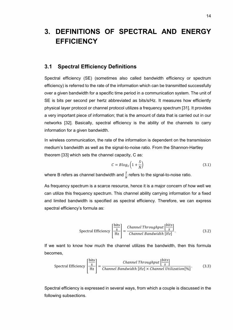
3.1 Spectral Efficiency Definitions
Spectral efficiency (SE) (sometimes also called bandwidth efficiency or spectrum
efficiency) is referred to the rate of the information which can be transmitted successfully
over a given bandwidth for a specific time period in a communication system. The unit of
SE is bits per second per hertz abbreviated as bits/s/Hz. It measures how efficiently
physical layer protocol or channel protocol utilizes a frequency spectrum [31]. It provides
a very important piece of information; that is the amount of data that is carried out in our
networks [32]. Basically, spectral efficiency is the ability of the channels to carry
information for a given bandwidth.
In wireless communication, the rate of the information is dependent on the transmission
medium’s bandwidth as well as the signal-to-noise ratio. From the Shannon-Hartley
theorem [33] which sets the channel capacity, C as:
𝐶 = 𝐵𝑙𝑜𝑔2 (1 +𝑆
𝑁) (3.1)
where B refers as channel bandwidth and 𝑆
𝑁 refers to the signal-to-noise ratio.
As frequency spectrum is a scarce resource, hence it is a major concern of how well we
can utilize this frequency spectrum. This channel ability carrying information for a fixed
and limited bandwidth is specified as spectral efficiency. Therefore, we can express
spectral efficiency’s formula as:
Spectral Efficiency [
bitss
Hz] =
𝐶ℎ𝑎𝑛𝑛𝑒𝑙 𝑇ℎ𝑟𝑜𝑢𝑔ℎ𝑝𝑢𝑡 [𝑏𝑖𝑡𝑠
𝑠]
𝐶ℎ𝑎𝑛𝑛𝑒𝑙 𝐵𝑎𝑛𝑑𝑤𝑖𝑑𝑡ℎ [𝐻𝑧]. (3.2)
If we want to know how much the channel utilizes the bandwidth, then this formula
becomes,
Spectral Efficiency [
bitss
Hz] =
𝐶ℎ𝑎𝑛𝑛𝑒𝑙 𝑇ℎ𝑟𝑜𝑢𝑔ℎ𝑝𝑢𝑡 [𝑏𝑖𝑡𝑠
𝑠]
𝐶ℎ𝑎𝑛𝑛𝑒𝑙 𝐵𝑎𝑛𝑑𝑤𝑖𝑑𝑡ℎ [𝐻𝑧] × 𝐶ℎ𝑎𝑛𝑛𝑒𝑙 𝑈𝑡𝑖𝑙𝑖𝑧𝑎𝑡𝑖𝑜𝑛[%]. (3.3)
Spectral efficiency is expressed in several ways, from which a couple is discussed in the
following subsections.

15
3.1.1 Link Spectral Efficiency
Link spectral efficiency is the net bitrate (without error-correcting codes) or maximum
throughput over a given bandwidth in a digital communication system or data link. It is
used in digital modulation or link code to analyze efficiency. It can also be used with the
combination of forwarding error correction (FEC) code along with other physical layer
overhead.
3.1.2 Area Spectral Efficiency or System Spectral Efficiency
Area spectral efficiency or system spectral efficiency is the measurement of the amount
of the users or services which we need to provide simultaneous support with our limited
frequency bandwidth within a fixed geographic area. It’s measured in bits/s/Hz per unit
area.
3.2 Energy Efficiency
Based on the circuit power consumption model, energy efficiency has been defined here.
From all aspects of science and technology, the basic theory of energy efficiency refers
to how much energy something consumes while doing a certain unit of work [34]. The
unit of work is more or less the same in all fields though in wireless communication,
expressing one unit of work is not easy at all. We have to explain a few different things
before we can exactly give the definition of work. In general, the wireless network in a
certain area provides wireless connectivity by transporting bits from BS to UEs and vice
versa. For these bits, the user has to pay the bill. But the fact is, users are paying not
only for the bits they are delivering but also for using the network. All above, classifying
the performance of a cellular network is more challenging than it appears as the
performance can be measured in a variety of ways and eventually it affects the energy
efficiency in different ways [34]. Moreover, the most common and popular definitions of
energy efficiency of a cellular network can be defined as, “The energy efficiency of a
cellular network is the number of bits that can be reliably transmitted over per unit of
energy” [37]. From the definition, energy efficiency can be derived as,
Energy Efficiency (EE) =𝑇ℎ𝑟𝑜𝑢𝑔ℎ𝑝𝑢𝑡 [
𝑏𝑖𝑡𝑠
𝑐𝑒𝑙𝑙]
𝑃𝑜𝑤𝑒𝑟 𝐶𝑜𝑛𝑠𝑢𝑚𝑝𝑡𝑖𝑜𝑛[𝑊
𝑐𝑒𝑙𝑙]
(3.4)
where throughput is the measure of the amount of data(bits) move successfully from one
place to another in a given time period [35] (typically measured in bits per second(bps),

16
as in megabits per second (Mbps) or gigabits per second (Gbps)). Moreover, power
consumption from the perspective of electrical engineering refers to the electrical energy
per unit time supplied to operate something [36]. It is usually measured in watts (W) or
in bigger volume, kilowatts (kW).
The unit of energy efficiency is bit/Joule. And this definition is also known as the benefit-
cost ratio, as the ratio is between the throughput and power consumption which means,
the quality of service (throughput) is being calculated with associated costs (power
consumption) [37].
Changes in the numerator and denominator affect the EE metric since both are
variable, which ensure that caution is taken to prevent the incomplete and possibly fals
e findings of the EE assessment. Especially, concentration should be emphasized more
and more when we do modeling of the power consumption (PC) of the network.
Sometimes, we assume that power consumption in a wireless network only comprises
transmit power, but this is a completely wrong conception. In [47], it has shown that we
can reduce transmit power towards zero as 1/√𝑀 when M→ ∞ while approaching a non-
zero asymptotic downlink (DL) spectral efficiency limit, which is misleading. The real fact
is that transmit power is a part of the overall power consumption.
Figure 5 shows the power consumption of the different parts of the coverage tier Base
Station. Data has been collected from [38].
Figure 5. Power consumed in percentage by different components of BS coverage tier
Power Supply (8 %) Signal Processing (10%)
Air Cooling (17%)
Power Amplifier

17
To compute network power consumption, we have to calculate the effective transmit
power (ETP) which is necessary, because it calculates the efficiency of the power
amplifier (PA). The efficiency of the power amplifier is vital because when the efficiency
of the power amplifier is low, that indicates a huge portion of the supply power is
dissipated as heat. Hence, we can calculate the power consumption of the Network like,
𝑃𝑜𝑤𝑒𝑟 𝐶𝑜𝑛𝑠𝑢𝑚𝑝𝑡𝑖𝑜𝑛 (𝑃𝐶) = Effective Transmit Power (ETP) + Circuit Power (CP) (3.5)
where the effective transmit power (ETP) refers to the exact amount of energy needed
to successfully transport a data package of a fixed number of bits from one palace. In
addition, circuit power refers to the energy consumed but the base station for control
signaling, backhaul infrastructure and load-independent power of the baseband
processors. It is a constant quantity which consumes almost one-quarter of the total
consumed power [figure 5]. Therefore, a common form of circuit power stands as,
Circuit Power (CP) = 𝑃𝐹𝐼𝑋 . (3.6)
This is not precise enough for comparing systems with various hardware configurations
and variable network loads because the energy dissipation of the analog hardware and
the digital signal processing is not accountable to it. Consequently, a too simplistic CP
model may lead to incorrect findings in many respects. For the evaluation of energy
consumption by a practical network and the identification of non-negligible parts, detailed
CP models are required.
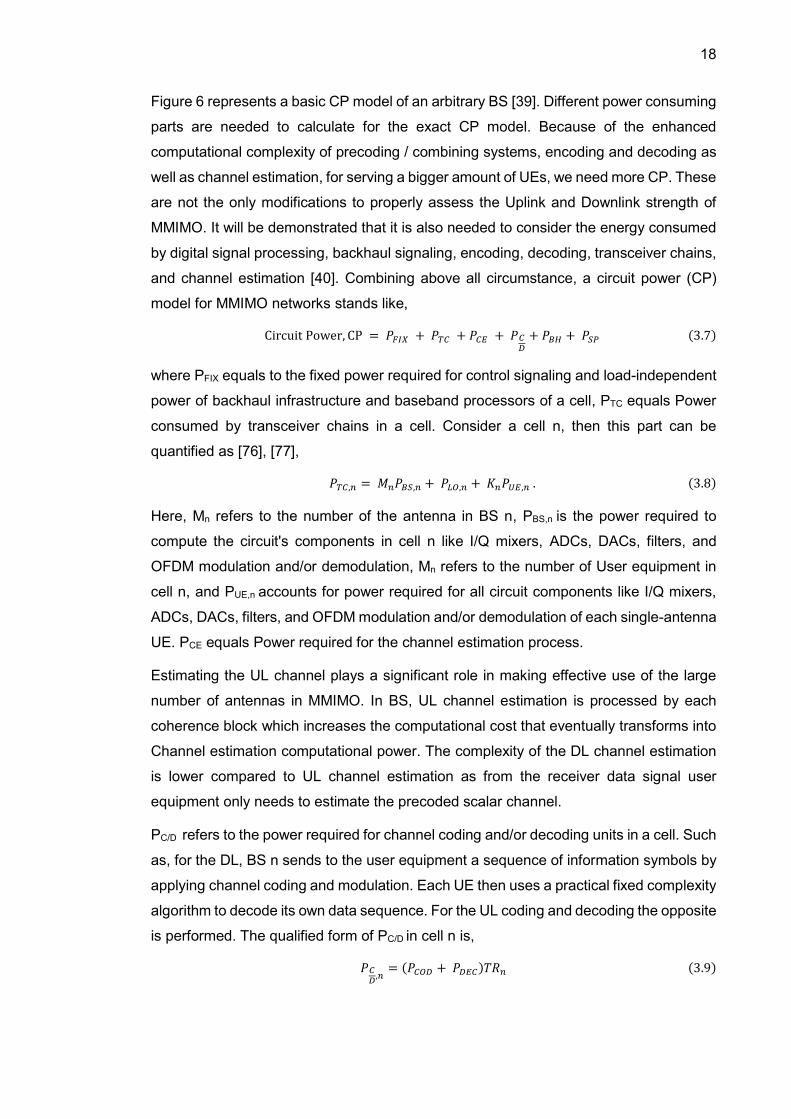
Figure 6. Basic block diagram of coverage BS’s power-consuming hardware element
18
Figure 6 represents a basic CP model of an arbitrary BS [39]. Different power consuming
parts are needed to calculate for the exact CP model. Because of the enhanced
computational complexity of precoding / combining systems, encoding and decoding as
well as channel estimation, for serving a bigger amount of UEs, we need more CP. These
are not the only modifications to properly assess the Uplink and Downlink strength of
MMIMO. It will be demonstrated that it is also needed to consider the energy consumed
by digital signal processing, backhaul signaling, encoding, decoding, transceiver chains,
and channel estimation [40]. Combining above all circumstance, a circuit power (CP)
model for MMIMO networks stands like,
Circuit Power, CP = 𝑃𝐹𝐼𝑋 + 𝑃𝑇𝐶 + 𝑃𝐶𝐸 + 𝑃𝐶𝐷
+ 𝑃𝐵𝐻 + 𝑃𝑆𝑃 (3.7)
where PFIX equals to the fixed power required for control signaling and load-independent
power of backhaul infrastructure and baseband processors of a cell, PTC equals Power
consumed by transceiver chains in a cell. Consider a cell n, then this part can be
quantified as [76], [77],
𝑃𝑇𝐶,𝑛 = 𝑀𝑛𝑃𝐵𝑆,𝑛 + 𝑃𝐿𝑂,𝑛 + 𝐾𝑛𝑃𝑈𝐸,𝑛 . (3.8)
Here, Mn refers to the number of the antenna in BS n, PBS,n is the power required to
compute the circuit's components in cell n like I/Q mixers, ADCs, DACs, filters, and
OFDM modulation and/or demodulation, Mn refers to the number of User equipment in
cell n, and PUE,n accounts for power required for all circuit components like I/Q mixers,
ADCs, DACs, filters, and OFDM modulation and/or demodulation of each single-antenna
UE. PCE equals Power required for the channel estimation process.
Estimating the UL channel plays a significant role in making effective use of the large
number of antennas in MMIMO. In BS, UL channel estimation is processed by each
coherence block which increases the computational cost that eventually transforms into
Channel estimation computational power. The complexity of the DL channel estimation
is lower compared to UL channel estimation as from the receiver data signal user
equipment only needs to estimate the precoded scalar channel.
PC/D refers to the power required for channel coding and/or decoding units in a cell. Such
as, for the DL, BS n sends to the user equipment a sequence of information symbols by
applying channel coding and modulation. Each UE then uses a practical fixed complexity
algorithm to decode its own data sequence. For the UL coding and decoding the opposite
is performed. The qualified form of PC/D in cell n is,
𝑃𝐶𝐷
,𝑛= (𝑃𝐶𝑂𝐷 + 𝑃𝐷𝐸𝐶)𝑇𝑅𝑛 (3.9)

19
where PCOD and PDEC are the respectively coding and decoding power(W/bit/s) and TRn
is the throughput(bit/s) of the cell n [41].
PBH refers to the power required to calculate load-dependent backhaul signaling.
Backhaul is the data transferring process. Depending on the network deployment it can
be either wired or wireless. It basically transports DL or UL data from BS to the core
network and vice versa. Backhaul can be classified into two parts. Load-independent
and Load-dependent backhaul. Load-independent backhaul is included in the PFIX part
of a cell and it consumes the most power (around 80%). On the other hand, the Load-
dependent backhaul of each BS is proportional to the sum throughput of its served UE.
It can be computed for cell n as,
𝑃𝐵𝐻,𝑛 = 𝑃𝐵𝑇 ∗ 𝑇𝑅𝑛 . (3.10)
As we already know, TRn is the throughput(bit/s) of the cell n and PBT is the backhaul
traffic power(W/bit/s) and for simplicity, it assumes to be the same in all cells.
PSP refers to the power required to processing the signal (receive combining and transmit
precoding) at the base station. To calculate PSP, computational complexity analysis has
been done in [42]. It can be shown for cell n as,
𝑃𝑆𝑃,𝑛 = 𝑃𝑆𝑃−
𝑅𝑇
,𝑛 + 𝑃𝑆𝑃−𝐶,𝑛
𝑈𝐿 + 𝑃𝑆𝑃−𝐶,𝑛𝐷𝐿 . (3.11)
Here, PSP-R/T,n refers to the total power consumed for a given combining and precoding
vector by DL transmission and UL reception. PSP-CUL
,n, and PSP-CDL
,n are the power
required in the cell n for calculating combining and precoding vectors respectively.
For small Multiuser MIMO, these transceiver chains, channel estimation, precoding, and
decoding power consumption are neglected. For the limited number of UEs and
antennas, these parts of the circuit power consumption are negligible compared to the
power consumed by the fixed part power consumption. However, after introducing the
MMIMO system, these parts of the circuit power consumption are considered both in
single-cell systems [43],[44],[45] and multi-cell systems [46].

20
4. SIMULATIONS TO ENHANCE SPECTRAL &
ENERGY EFFICIENCY
4.1 Achievable Uplink Spectral Efficiency
From the perspective of the wireless networks, by linear receiving combining scheme,
any BS can detect their desire signal. Any BS can receive a signal from UE by selecting
the combining vector as a function of channel estimator which is acquired from the pilot
transmission. At the time of data transmission, any BS can correlate received signal and
this combining vector by summing the desired signal over the estimated channel, desired
signal over an unknown channel, intra-cell interference, inter-cell interference and noise
[48].
For a random cell j, if MMSE channel estimator is considered for UL ergodic channel
capacity of a random UE k, then lower bounded SE for UL would be like:
𝑆𝐸𝑗𝑘𝑈𝐿 =
τu
τc
𝔼 {log2(1 + 𝑆𝐼𝑁𝑅𝑗𝑘𝑈𝐿)} (4.1)
where SINRjkUL is UL instantaneous SINR though it is not conventional sense,τu is the
UL data samples per coherence block, τc is the number of samples per coherence block
and together τu
τc is a pre-log factor that a fraction of the samples per coherence block that
are used for uplink data. From this SE equation, SE for UL can be achieved.
From this lower bounded SE for UL formula, UL data samples per coherence block, τu =
τc - 𝜏𝑝 - 𝜏𝑑. Where 𝜏𝑝 is the number of samples allocated for pilots per coherence block,
and 𝜏𝑑 donates for DL data samples per coherence block. Hence, SE of cell j for the kth
UE can be increased if the per-log factor is increased. This can be performed if the
reduction is made in the 𝜏𝑑 and/or shorten the 𝜏𝑝 length [49].
In order to exemplify the SE and how to increase it in the simulation and results part,
values have been taken from [50, table 4.2] for MMIMO. Considering 16 (4 * 4) cell wrap-
around network layout is taken, and the coverage of each cell is considered
0.25km*0.25km. The reason for using wrap around the technology is so that interference
from all surrounding can be received by all BSs. Taking a shorter distance from UE to
BS, a large-scale fading model is used. For MMIMO, the communication bandwidth of
20 MHz is considered and for NB-IoT, 200 kHz is taken. For MMIMO, UL transmit power
per UE is considered as 20 dBm and for NB-IoT it has taken 23 dBm. On the other hand,

21
for DL transmission, MMIMO is considered 20 dBm while NB-IoT is considered 43 dBm
per UE from BS [51]. For calculation, 2 sets of data are considered (for MMIMO and NB-
IoT) from [48],[49],[52]. As the simulation has performed for UL, the receiver noise power
is taken from the UL frequency of NB-IoT (15 kHz).
Table 2. System parameters regarding MMIMO and NB-IoT.
Parameter Value of MMIMO Value of NB-IoT
UL transmit Power 20 dBm 23 dBm
DL transmit Power 20 dBm 43 dBm
Bandwidth 20 MHz 200 kHz
Shadow fading (standard deviation) 10 10
Pathloss exponent 3.76 3.76
Receiver Noise Power -94 dBm -129 dBm
(for 15 KHz)
Samples per coherence block 200 200
Pilot reuse factor f = 1, 2, 4 f = 1, 2, 4
Number of pilot sequences f*K f*K
Coherence block, τc consist of 200 samples, considering M antennas in each BS and K
UEs per cell. Changing the value of M and K and taking the ratio of M/K simulation has
performed for results. Pilot sequence, 𝜏𝑝 is used in different ways among the UEs and
calculated the multiplication of pilot reused factor, f and number of UEs, K. To simplify
the calculation and simulation pilot reused factor has taken as, f = {1, 2, 4}. In every cell,
these pilots are assigned randomly for the UEs.
With all of these values, in [50], the simulation has done for MMIMO average sum SE
which is a function of a number of BS antennas for different combining schemes [48,
figure 4.5]). The simulation has done here for calculations and coming to the conclusion
(figure 7). From figure 7, information can be extracted that with the pilot reused factor, f
equals 1, M-MMSE receiving combing schemes provides the highest SE followed by S-
MMSE. SE is reduced with every other scheme after M-MMSE.
22
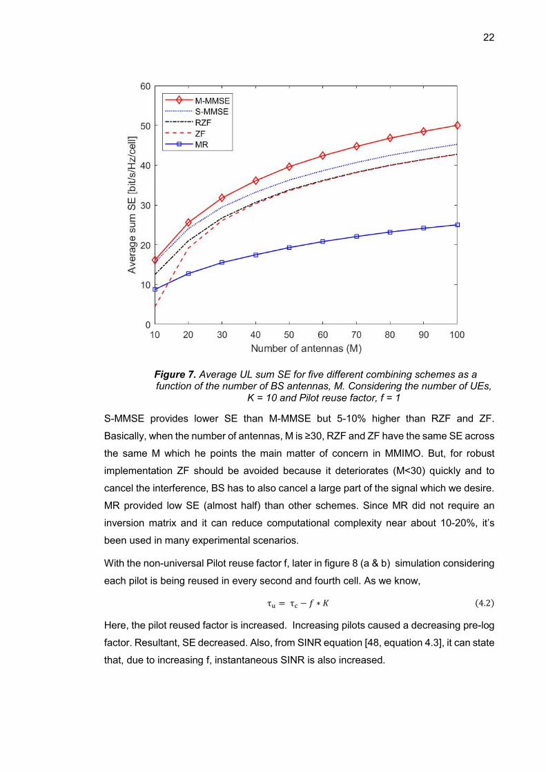
Figure 7. Average UL sum SE for five different combining schemes as a function of the number of BS antennas, M. Considering the number of UEs,
K = 10 and Pilot reuse factor, f = 1
S-MMSE provides lower SE than M-MMSE but 5-10% higher than RZF and ZF.
Basically, when the number of antennas, M is ≥30, RZF and ZF have the same SE across
the same M which he points the main matter of concern in MMIMO. But, for robust
implementation ZF should be avoided because it deteriorates (M<30) quickly and to
cancel the interference, BS has to also cancel a large part of the signal which we desire.
MR provided low SE (almost half) than other schemes. Since MR did not require an
inversion matrix and it can reduce computational complexity near about 10-20%, it’s
been used in many experimental scenarios.
With the non-universal Pilot reuse factor f, later in figure 8 (a & b) simulation considering
each pilot is being reused in every second and fourth cell. As we know,
τu = τc − 𝑓 ∗ 𝐾 (4.2)
Here, the pilot reused factor is increased. Increasing pilots caused a decreasing pre-log
factor. Resultant, SE decreased. Also, from SINR equation [48, equation 4.3], it can state
that, due to increasing f, instantaneous SINR is also increased.
23
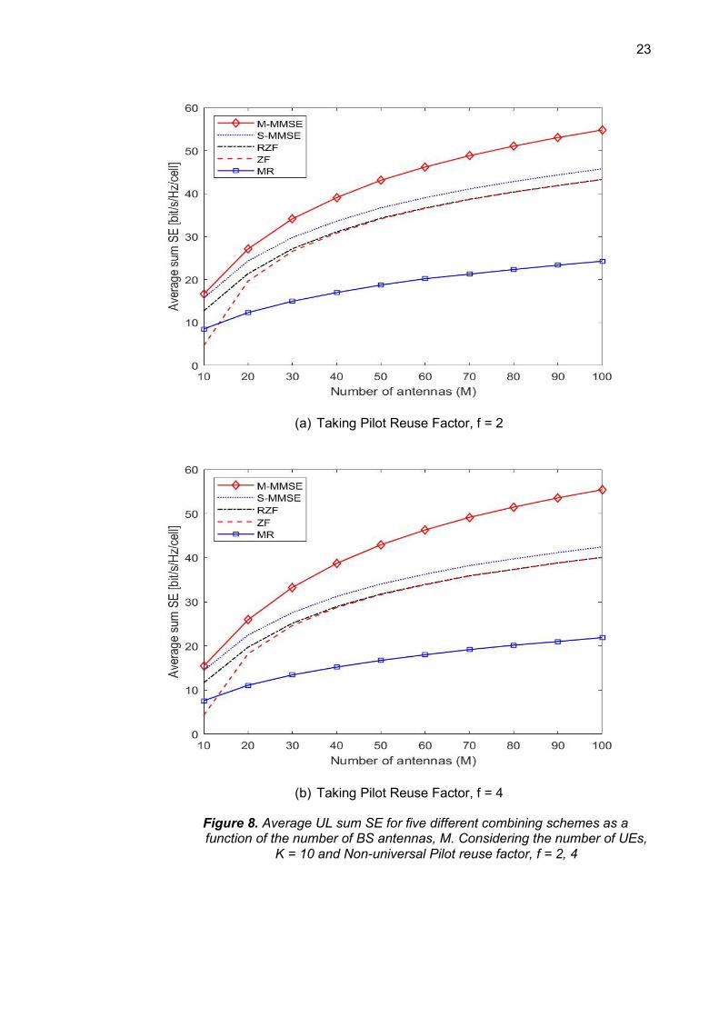
(a) Taking Pilot Reuse Factor, f = 2
(b) Taking Pilot Reuse Factor, f = 4
Figure 8. Average UL sum SE for five different combining schemes as a function of the number of BS antennas, M. Considering the number of UEs,
K = 10 and Non-universal Pilot reuse factor, f = 2, 4
24
The explanation can be given from figures 8a and 8b that, for M-MMSE increasing the
pilot reuse factor has more benefits in SE since it can suppress the interference from
UEs in the neighbor cells as other pilots have been used by these UEs. For comparison,
the data table for different receiving combining schemes with different pilot reuse factor
is given below in table 3.
Table 3. Average UL sum SE [bits/s/Hz/cell] for different pilot reuse factors.
Combining Schemes f = 1 f = 2 f = 4
M-MMSE 50.32 55.10 55.41
S-MMSE 45.39 45.83 42.41
RZF 42.83 43.37 39.99
ZF 42.80 43.34 39.97
MR 25.25 24.41 21.95
With increasing f, the M-MMSE scheme gives better SE than before. For S-MMSE, RZF,
and ZF, SE increases up to f = 2, then it starts falling down with increasing f. The highest
SE value among these three is obtained when f = 2. The scenario is different in the case
of MR. It gives the highest sum SE at f = 1 and with increasing pilot reuse factor, MR
reduces. The reason behind that is since the estimation is only related to coherently
combine the desired signal and not used to cancel interference, hence improved quality
of estimation can’t outweigh the pre-log factor which is reduced. Also, from table 3, it can
be seen that the highest sum SE is achieved at any f for M-MMSE compared to others.
For S-MMSE, RZF, and ZF this value belongs to f = 2 and for MR it remains in f = 1.
The main reason behind these 5 different schemes description is to choose which
schemes can be chosen for implementation. They are, M-MMSE, RZF, and MR. M-
MMSE gives the highest SE in all values of the pilot reuse factor, f in spite of having
computational complexity. MR has the lowest SE but has the lowest computational
complexity as well. RZF has a well balanced between SE and complexity. Its
computational complexity is only ten of a percentage higher than MR but has SE almost
double to MR. Though ZF has almost the same SE as RZF RZF is a better choice than
ZF when M ≈ K because at this stage ZF has serious robustness issues.
4.1.1 Impact of Spatial Channel Correlation
Spatial channel correlation has a significant impact on the quality of channel estimation,
channel hardening as well as propagation. Under spatial channel correlation, channel
estimation quality improves and more favorable propagation of the UEs has exhibited
which have different spatial characteristics.

25
Figure 9. Average UL sum SE using the Gaussian local scattering channel model as a function of varying ASD. Considering K =10 UEs, M = 100
antennas and the number of setups with random UE locations = 10. Three combining schemes are used, and the dotted lines represent achievable SE
with the aid of uncorrelated Rayleigh fading channels
Based on the SE-computational complexity tradeoff which has already done, the
simulation has done again for average UL sum SE as a function of Angular Standard
Deviation, 𝜎𝜑 with M-MMSE, RZF and MR combining with the help of data and code from
[48]. Considering the number of antennas, M = 100 in a BS equips with UEs, K = 10.
Varying 𝜎𝜑 from 0 to 50 to observe the impact in figure 9.
From the figure, it is observable that, M-MMSE has the highest SE for any value of ASD,
followed by RZF and after that MR. But, all of them, the common thing is, SE decreases
with increasing ASD. This is an indication of high spatial channel correlation’s dominant
effect which reduces interference between UEs that have different spatial correlation
matrices. With small ASD ( 𝜎𝜑≤10), the interference between UEs is low and LoS
scenario resembles there unless UEs have the same ASD from BS. It can also observe
that the SE performance order of both spatial channel correlation and combining
schemes remain the same. For 𝜎𝜑 ≤ 50, M-MMSE benefited from spatial correlation. The
performance of RZF and MR remain better if 𝜎𝜑 ≤ 20. Performance drops down

26
increasing 𝜎𝜑 afterward. If ASD is large enough then SE of these three schemes fall
slightly compared to the uncorrelated Rayleigh fading channel because of the geometry
of the uniformed linear array.
Therefore, a conclusion can be made that, ASD value should be kept smaller (within 10
to 20) for all three schemes in order to acquire the highest average UL sum SE.
4.1.2 Impact of Pilot Contamination and Coherent Interference
In UL, pilot contamination has few adverse effects. Firstly, due to the contamination, the
channel’s Mean-Square error (MSE) increases. As a result, it reduces the ability to
choose to combine vector which can provide strong array gains as well as can reject
non-coherent interference. And secondly, it raises the coherent interference which array
gain amplifies.
To examine the impact of pilot contamination, the simulation has performed in [50]
considering uncorrelated fading channel with the number of antennas, M = 100, UEs K
= 10, Gaussian local scattering channel model taking 𝜎𝜑 = 10. Estimation of the average
power of the signal, the coherent interference, and non-coherent interference have
estimated from Monte Carlo simulations. The average power of the strongest and the
weakest UEs are taken from a random cell just because of UEs locating various locations
display different power levels. UEs are responsible for non-coherent interference while
coherent interference is additional interference which is caused by the pilot
contaminating UEs. With respect to the noise power, all powers are normalized. For
examinations, simulations and results part, the simulation has performed taking into
account the number of setups with random UE locations equals 10 (figure 10).

27
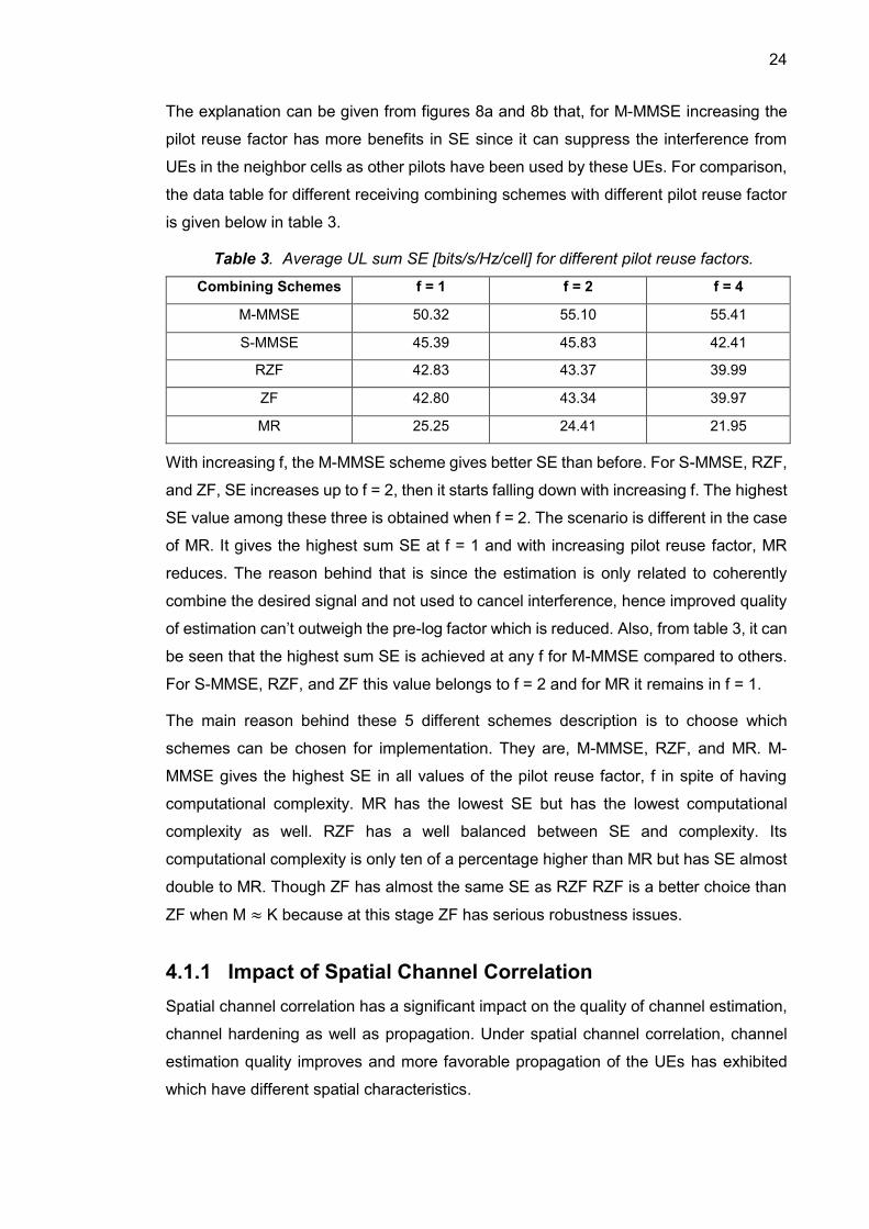
(a) Strongest UEs in the cell
(b) Weakest UEs in the cell
Figure 10. Average UL power of the desired signal with coherent interference and non-coherent interference
The simulation’s figure 10a has shown the signal power with coherent and non-coherent
interference for both the strongest and weakest (figure 10b) UEs of all the three
combining schemes. From the curve, the strongest UE has almost the same signal power
for any value of the pilot reuse factor. Hence, the impact on the MSC for the channel
estimator is very minor. The received desire signal has 25 dB higher signal power than
con-coherent interference and more than 40 dB higher power than coherent interference.
28
MR combining has provided the highest signal power, while to find combining vectors,
M-MMSE and RZF lose a few signal powers in order to suppress 10 dB or more
interference. Hence, the nutshell of the simulation is, as UEs, which causes interference
far away from receiving BS, coherent interference’s impact is negligible to the strongest
UEs than non-coherent interference.
Figure 10b shows the UEs which is located at the cell edge. Compared to the strongest
UE, additional path loss has decreased the signal’s power many tens of dB lower. The
quality of channel estimation is poor for that after receive combining the desired signal
power can be increased with the aid of larger f. MR has the strongest signal power though
it is almost 10 dB weaker than the non-coherent interference. As their present intra-cell
interference which can’t suppress. To find combining vector, RZF and M-MMSE sacrifice
a few dB of signal power which suppresses non-coherent interference by more than or
equals 10 dB. Hence, for calculating signal power for the weakest UEs, coherent
interference holds the dominant interference. For uncorrelated fading coherent
interference is almost the same for all schemes. But, increasing f, its dominant effect can
be diminished. In that sense, and for strongest UE, M-MMSE has the most beneficial
effect from increasing f as for suppressing inter-cell interference, it performs better.
To conclude, pilot contamination has an adverse impact on the cell edge UEs which
exhibit uncorrelated fading. But, a very low impact on the channel estimation quality. Pilot
contamination has given birth to Coherent interference. Coherent interference can be
stronger than the non-coherent interference in some cases when UEs are at the cell
edge and exhibit uncorrelated fading. However, it can be alleviated if the pilot reuse
factor can increase. The remaining pilot contamination’s impact lies in the pre-log factor
of SE. This can also be decreased as the number of pilots grow.
4.1.3 SE with Other Channel Estimation Schemes than MMSE
To compensate for the computational complexity with the aid of estimation quality
reduction, alternative EW-MMSE, as well as LS channel estimator, are proposed in [53].
To compare these different channel estimators, simulation has been executed. We have
tried to figure out the average UL sum SE by using MMSE, EW-MMSE, and LS.
Considering the number of BS antennas, M = 100 and K = 10 UEs simulation has been
done. The pilot reuse factor is used according to the combining schemes by which SE
becomes maximized From the simulation output and curves in figure 11, it has observed
a bar diagram of the average UL sum SE with M-MMSE, RZF, and MR combining
schemes.

29
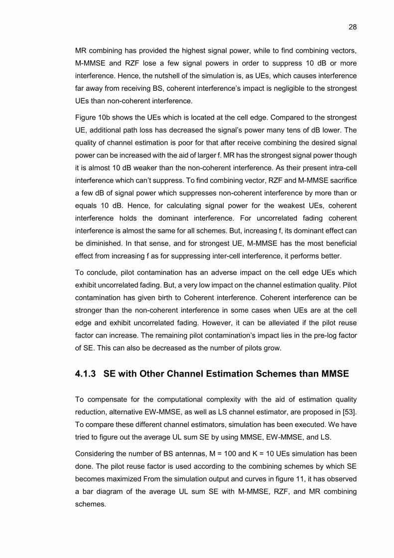
Figure 11. Average UL sum SE of M-MMSE, RZF, and MR combining by using MMSE, EW-MMSE, and LS estimator
From the figure, the highest SE is achieved by using the MMSE estimator followed by
the EW-MMSE estimator which has on average 8%-12% less SE depending on
combining schemes compared to MMSE. M-MMSE combining performance is very poor
in LS estimators but compared to EW-MMSE, RZF and MR have the same SE in both
cases. In the presence of pilot contamination, the LS estimator is unable to provide the
right scaling of the channel estimates. On the contrary, it acts like an estimator that sum
the interfering channel.
The main target is to obtain substantial SE gain irrespective of channel estimator. MMSE
provides better SE in all three schemes but introduces high complexity. Since high
complexity estimation schemes are tried to be avoided sometimes. In that case, EW-
MMSE can be a better option as it shows the good tradeoff between SE and complexity.
Hence, an alternative, EW-MMSE channel estimator can be a suitable preference if the
highest SE is not the priority. However, LS estimation should be avoided.
30
4.2 Energy Efficiency
4.2.1 Hotspot Tier
Hotspot tier is a part of the heterogeneous network. It consists of mainly indoor base
stations that provide high throughput within a small area. The mmWave bands are
congenial for it to improve throughput.
Hotspot BS has played an important role to reduce transmit power at the same time
increasing throughput. It basically provides additional capacity within the coverage tier
BSs by narrowing the distance between serving BSs and UEs [54]. The mechanism
behind hotspot BS is, deploying a wider range of network infrastructure and a large
amount of transceiver hardwires [55]. But deploying such a large number of transceivers
and network structure, it can increase the power consumption of the network, although
there remain various possible solutions. Sensor technology can be a possible solution
where hotspot BSs is equipped with a traffic load monitoring mechanism [56],[57], and
an automatic turn-on, turn-off components according to the demands. These
technologies are really efficient to reduce power consumption without losing area
throughput. But there remains a huge leakage, that is, these technologies degrade the
coverage the mobility support and coverage. Hence, it is not very suitable for the
operation of the coverage tier. Researches have been going over how to make the
consumed power equal to the network load so that the dynamic turn-on and turn-off can
be avoided.
Before making any network Energy Efficient, we have to know Area Transmit Power
(ATP), which is the network-average power uses for the sake of per area data
transmission. It is basically a metric that measures the consumed transmit power by the
wireless network. Therefore, it is described as,
𝐴𝑇𝑃 = 𝑃 ∗ 𝐷 (4.3)
where P is the transmit power (W/cell) and D is the average cell density in the unit area
(cells/km2). The unit of ATP is W/km2.
Now, for ATP for UL in MMIMO, if a network is considered which is equipped with L cells,
number of BS j, and K UEs, and if BS j wants to communicate with Kj UEs, pjK is the
signal variance, then, ATP of the BSj for UL becomes,
𝐴𝑇𝑃𝐽𝑈𝐿 = 𝐷 ∑ 𝑃𝑗𝐾
𝐾𝑗
𝐾=1 . (4.4)
For the corresponding ATP for DL, 𝐴𝑇𝑃𝐽𝐷𝐿 can be achieved only by replacing PjK by 𝜌𝑗𝐾.
If we want to calculate 𝐴𝑇𝑃𝐽𝐷𝐿 or 𝐴𝑇𝑃𝐽
𝑈𝐿 (both would be same as both needs transmit

31
power to 20 dBm for MMIMO), considering K equals 10 UEs, pilot reuse factor, f equals
1, 4 by 4 cells, BS coverage area of (0.25*0.25) km2, and number of antennas, M, then
the total transmit power would be = 100 mW * 10 = 1000 mW = 1W = 30 dBm. Therefore,
𝐴𝑇𝑃𝐽𝐷𝐿 would be = (4*4) *1 = 16W/km2.The same result would be achievable for 𝐴𝑇𝑃𝐽
𝑈𝐿.
Compared to the LTE network this UL or DL ATP is much smaller.
Table 4. Average DL throughput over 20 MHz channels per cell.
Schemes M = 10 M = 50 M = 100
M-MMSE 243 Mbit/s 795 Mbit/s 1053 Mbit/s
RZF 217 Mbit/s 648 Mbit/s 832 Mbit/s
MR 118 Mbit/s 345 Mbit/s 482 Mbit/s
Table 4 represents the average DL throughput for M-MMSE, RZF, and MR combining
over 20 MHz channels per cell. Values are collected from [48]. From the table it can
experience, M-MMSE, as expected, has the highest throughput for every number of BS
antenna. For, M = 100, M-MMSE and MR have DL throughput of 1053 Mbit/s and 482
Mbit/s respectively which is almost 10 times higher than LTE [58]. Hence, total area
throughput of M-MMSE become 3.88 Gbit/s/km2, 12.72 Gbit/s/km2 and 16.8 Gbit/s/km2
for M = 10, 50 and 100 respectively.
Hence, with a large number of BS antennas, MMIMO can achieve much higher
throughput and an-order-of magnitude ATP savings than LTE at the same time. Besides
total transmit power divides among all the antennas M, resultant transmit power per
antenna is very low. As it can be seen from here, if the total 1W transmit power is divided
among 100 antennas, then only 10mW per antenna for transmission is consumed. As
transmit power per antenna is low, we don’t need to use high power-consuming PAs
which are being used in the traditional cellular networks. Operators can replace them
with hundreds of low powers (~mW range) and low-cost PAs.
One and most important drawback of ATP metric is that it increases the circuit power of
the network. Since, for this setup, we need to deploy multiple RF chains,
precoding/combining schemes, in each BS. For that, the computational complexity
becomes much higher depending on the number of UEs and BS antennas, M and
resultant increases CP. As a result, to make the network energy efficient which is the
main motto of this thesis remains under obstacle. For that EE metric can be a better
choice than ATP metric.

32
4.2.2 Asymptotic Analysis of Transmit Power
Asymptotic analysis means calculating the operating time of an algorithm in
mathematical units of computation. It basically mentions an algorithm’s mathematical
boundation or framing according to its run-time performance [66]. After performing
asymptotic analysis, the algorithm’s case scenario ( the best case, average case or worst
case) can be judged.
The explanation of asymptotic analysis of the transmit power has given about the impact
in EE when the number of antennas grows higher. It will see the CP performance when
Mj → ∞ in the asymptotic regime while keeping the number of UEs, K fixed. MMIMO can
be operated at really very small transmit power levels. In theoretical assumption,
approaching toward a non-zero SE, transmit power can asymptotically become zero.
To reach the asymptotic non-zero limit, a calculation has performed in [50] with DL
transmit power and considering MR schemes. As other precoding and combining
schemes have better and larger SE value than MR, that’s why he establishes with MR
so that other schemes can hold the same result as well. With MR precoding, having K
UEs in cell j has DL channel capacity which is lower bounded by,
𝑆𝐸𝐽𝐾𝐷𝐿 =
𝜏𝑑
𝜏𝑐
𝑙𝑜𝑔2(1 + 𝑆𝐼𝑁𝑅𝐽𝐾𝐷𝐿) (4.5)
where this term 𝑆𝐼𝑁𝑅𝑗𝐾𝐷𝐿 has derived from [48, equation 5.4].
[48, lemma 5.1] has shown transmit power scaling low for MMIMO networks, where the
conditions are,
M → ∞ if ∈1+∈2 < 1
while 𝑆𝐼𝑁𝑅𝑗𝐾𝐷𝐿 → 0 if ∈1+∈2 > 1.
The condition ∈1+∈2 < 1 implies that, either both UL and DL transmit power pjK and
𝜌𝑗𝐾 should decrease roughly as 1/√𝑀 or, or we can decrease one faster, one slower
until the product PjK*𝜌𝑗𝐾 doesn’t decay faster than 1/M.
From the power scaling low, if transmit power can be reduced faster than these two
conditions, then zero asymptotic SE is achievable.
To exemplify this asymptotic result, simulation has performed with the lemma 5.1 taking
MR precoding. Assuming ∈ = ∈1 =∈2, number of UEs, K = 10, UL/DL transmit power per
UE, 𝑃 = 𝑃 = 20 dBm, total DL transmit power, K𝑃 = 30 dBm, ∈ = 1/2 , ∈ = 1 and ∈ = 0.
Considered Uncorrelated Rayleigh fading showed in figure 12.

33
Figure 12. Average DL sum SE with normalized MR precoding as a function of
the number of antennas, M. Taking 𝑃 = 𝑃 = 20 dBm ; fixed power (i.e., ∈ =
0), ∈ = ½ and ∈ = 1; Considering Uncorrelated Rayleigh fading.
From figure 12, it can be shown that, when ∈ = ½ i.e., PjK and 𝜌𝑗𝐾 decrease as 1/√𝑀,
DL sum SE approaches towards the non-zero asymptotic limit. The behavior is
somewhat almost similar to fixed power (when ∈ = 0). 55% asymptotic value is obtained
when the number of antennas, M =103 i.e., 1000. While almost 95% asymptotic value
can be achieved with M = 106 i.e., 1,000,000. When ∈ = 1, the average DL sum SE
vanishes.
In addition, when M = 100, the total transmit power of BS decreases from 1W to K𝑃/√𝑀
= 0.1W.
Dividing this 0.1W among 100 transmitting antennas, 1 mW power is needed to operate
each antenna. This clearly indicates that, theoretically, MMIMO can be operated at low
transmit power, keeping the same SE values. Although this transmits power reduction
comes for deploying more BSs antennas which increase circuit power eventually.

34
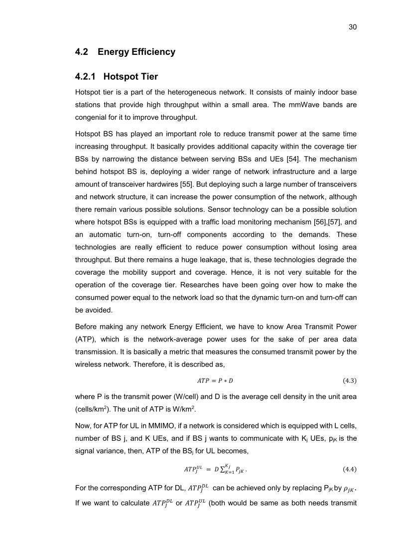
5. SIMULATIONS AND RESULTS
Massive MIMO and NB-IoT can certainly improve the network efficiency of the cellular
network. Whereas, at the same time, increasing the performance of spectral efficiency
substantially degrades the energy efficiency due to the huge number of RF chains and
PAs. Experimenting the spectral and energy efficiencies along with RF chains, power
amplifiers, base station’s power consumption, precoding and combining schemes and
so on, it has shown that there exists an optimal point, where it is possible to maintain the
energy efficiency without decreasing the spectral efficiency as well as throughput. For
the simulation purposes, a general form of 20 MHz band MMIMO network is considered
which is mathematically more convenient to study and MATLAB simulations have
performed by using data from [48]. From [59], the upper bound of the energy efficiency
is derived as,
𝜂�̂�𝐹 =K𝑙𝑜𝑔2 [1 + (
𝑃𝑂𝑈𝑇K ) ∗ (
𝑁𝑇𝑋𝜋2 − 𝜋 + 44 )]
1𝛼 𝑃𝑂𝑈𝑇 + 𝐾((𝑃𝑅𝐹 + 𝑃𝐵𝐵) + 𝑃’𝐶
(5.1)
where K is the total number of Users Equipment, POUT is the BS downlink transmit power,
PRF is the power consumed by RF chains, PBB is the power consumed for the baseband
processing, P’C is the fixed power consumption by BS not including the power consumed
for downlink transmission, NTX is the number of transmitting antennas in BS.
Implementing this algorithm in Matlab and then the result has illustrated in figure 13. The
energy efficiency as a function of the number of transmitting antennas in a single BS, the
first assumption is that, with increasing the number of transmitters energy efficiency
increases. At first, when the number of transmitters rises from 1 to 20, energy efficiency
increases rapidly. After that, the increment of EE is smoother and gradual. From 1 to 40
transmitters, EE increasing rate is high and after that, it becomes gradual and smooth.
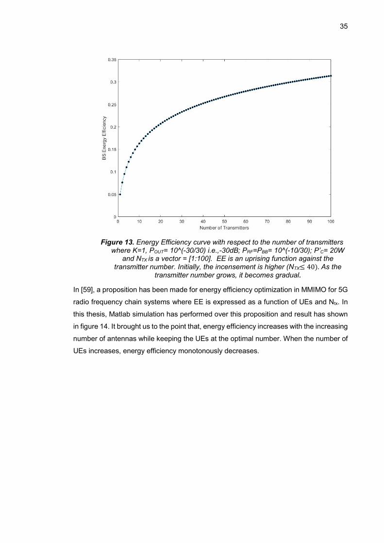
35
Figure 13. Energy Efficiency curve with respect to the number of transmitters
where K=1, POUT= 10^(-30/30) i.e.,-30dB; PRF=PBB= 10^(-10/30); P’C= 20W and NTX is a vector = [1:100]. EE is an uprising function against the
transmitter number. Initially, the incensement is higher (NTX≤ 40). As the transmitter number grows, it becomes gradual.
In [59], a proposition has been made for energy efficiency optimization in MMIMO for 5G
radio frequency chain systems where EE is expressed as a function of UEs and Ntx. In
this thesis, Matlab simulation has performed over this proposition and result has shown
in figure 14. It brought us to the point that, energy efficiency increases with the increasing
number of antennas while keeping the UEs at the optimal number. When the number of
UEs increases, energy efficiency monotonously decreases.

36
Figure 14. G(K, NTX) as a function of UEs with respect to the number of antennas. K is a vector = [1:100], POUT= 10^(-30/30) i.e.,-30dB; PRF=PBB=
10^(-10/30); P’C= 20W and NTX is a vector = [1:100]. The function is monotonically decreasing with relevant to the number of antennas, NTX.
Also, it decreases gradually while increasing the number of UEs.
To explore into more detail calculations considering various network parameters under
different operating conditions, first, it has examined the two-cell Wyner model for UL [60].
From [60], the number of UE in cell 1 is 1, assuming no Inter-cell Interference (ISI) from
cell 2 and considering Rayleigh fading channels, SE and EE have calculated from cell 1
as,
𝑆𝐸 = [1 + (𝑀 − 1)𝑝
𝜎2 𝛽] (5.2)
𝐸𝐸 = 𝐵 ∗ 𝑆𝐸
(2𝑆𝐸 − 1)𝜗
(𝑀 − 1)+ 𝑃𝐹𝐼𝑋
. (5.3)
Form the above expressions, calculating them and doing simulation the maximum
tradeoff of EE and SE for cell 1 (Figure 15) has obtained. The maximum tradeoff has
been achieved as it has only considered the basic model ignoring fading, non-line-of-
sight (NLoS), ISI and RF chains power consumption in BS.
According to the [60], the Maximum EE(EE*) and maximum SE(SE*) in cell 1 satisfy the
identity as,
𝑙𝑜𝑔2(𝐸𝐸∗) + 𝑆𝐸∗ = 𝑙𝑜𝑔2 [(𝑀 − 1)𝐵
𝜗𝑙𝑜𝑔2(2)] . (5.4)
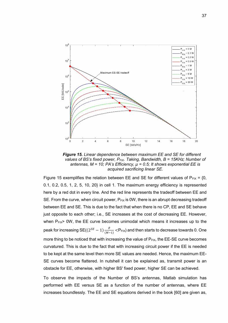
37
Figure 15. Linear dependence between maximum EE and SE for different values of BS’s fixed power, PFIX. Taking, Bandwidth, B = 15KHz; Number of
antennas, M = 10; PA’s Efficiency, µ = 0.5; It shows exponential EE is acquired sacrificing linear SE.
Figure 15 exemplifies the relation between EE and SE for different values of PFIX = {0,
0.1, 0.2, 0.5, 1, 2, 5, 10, 20} in cell 1. The maximum energy efficiency is represented
here by a red dot in every line. And the red line represents the tradeoff between EE and
SE. From the curve, when circuit power, PFIX is 0W, there is an abrupt decreasing tradeoff
between EE and SE. This is due to the fact that when there is no CP, EE and SE behave
just opposite to each other; i.e., SE increases at the cost of decreasing EE. However,
when PFIX> 0W, the EE curve becomes unimodal which means it increases up to the
peak for increasing SE((2𝑆𝐸 − 1)𝜗
(𝑀−1)<PFIX) and then starts to decrease towards 0. One
more thing to be noticed that with increasing the value of PFIX, the EE-SE curve becomes
curvatured. This is due to the fact that with increasing circuit power if the EE is needed
to be kept at the same level then more SE values are needed. Hence, the maximum EE-
SE curves become flattered. In nutshell it can be explained as, transmit power is an
obstacle for EE, otherwise, with higher BS' fixed power, higher SE can be achieved.
To observe the impacts of the Number of BS’s antennas, Matlab simulation has
performed with EE versus SE as a function of the number of antennas, where EE
increases boundlessly. The EE and SE equations derived in the book [60] are given as,
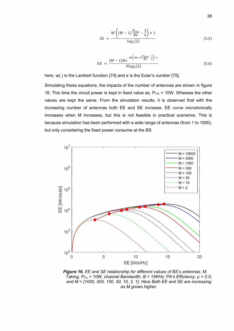
38
𝑆𝐸 =
𝑊 ((𝑀 − 1)𝑃𝐹𝐼𝑋
𝜗𝑒 –
1𝑒
) + 1
𝑙𝑜𝑔2(2) (5.5)
𝐸𝐸 = (𝑀 − 1)𝐵𝑒
−𝑊((𝑀−1)𝑃𝐹𝐼𝑋
𝜗𝑒 –
1𝑒
)−1
𝜗𝑙𝑜𝑔2(2) (5.6)
here, w(.) is the Lambert function [74] and e is the Euler’s number [75].
Simulating these equations, the impacts of the number of antennas are shown in figure
16. This time the circuit power is kept in fixed value as, PFIX = 10W. Whereas the other
values are kept the same. From the simulation results, it is observed that with the
increasing number of antennas both EE and SE increase. EE curve monotonically
increases when M increases, but this is not feasible in practical scenarios. This is
because simulation has been performed with a wide range of antennas (from 1 to 1000),
but only considering the fixed power consume at the BS.
Figure 16. EE and SE relationship for different values of BS’s antennas, M. Taking, PFix = 10W, channel Bandwidth, B = 15KHz; PA’s Efficiency, µ = 0.5; and M = [1000, 500, 100, 50, 10, 2, 1]. Here Both EE and SE are increasing
as M grows higher.

39
In MMIMO, each and every antenna is equipped with RF chains and PAs. These things
consume power which can not be ignored when calculating the number of antennas like
50, 100, 500 or 1000. Hence for basic and simple understanding, increasing the BS
transmitting antennas, both EE and SE increase unless the total power consumption is
considered.
When the EE-SE tradeoff exemplifies, the impact of the noise power, 𝜎2 and the average
channel gain of the active UEs, 𝛽 should be considered. In all these simulations, the
value of 𝜎2/ 𝛽 is defined as -6dBm as it is the most common case considering 20 MHz
band cellular MMIMO. Here, simulation has been performed by taking into account
different 𝜎2/𝛽 values which has shown in figure 17. The same equations of SE and EE,
which have used to illustrate EE and SE relationship for different values of BS’s
antennas, have been used here. In this case, the number of antennas kept fixed as, M =
10,000.
Figure 17. EE versus SE relation for different 𝜎2/ 𝛽 values. Keeping PFix = 10W, channel Bandwidth, B = 15KHz; PA’s Efficiency, µ = 0.5; and M =
10000. We have taken value as [-2, -3, -4, -5, -6, -7, -8, -9].

40
Figure 17 illustrates, changing the ratio value between signal power and average channel
gain per active UE, it is observed that EE increases when the value of 𝜎2/ 𝛽 decreases.
This indicates that in order to glorify EE, the average channel gain fo the active UE’s
needs to increase and at the same time, the signal noise power needs to decrease. The
MMIMO’s assume UL bandwidth is 100 kHz, whereas in NB-IoT, for UL, the bandwidth
is 15KHz bandwidth. As from equations,
Noise Power = 𝐾𝑏 ∗ T ∗ B (5.7)
where Kb is the Boltzmann constant of value 1.38*10-23 J/K, T is the absolute temperature
of the device which is approximate ~ 273.15K and B is the channel bandwidth. Here, if
Kb and T are considered as constant quantity, then the noise power is totally dependent
on B. Hence if channel BW is smaller (such as NB-IoT), the system’s noise power will be
less. For example, if calculation is done for the noise power of MMIMO and NB-IoT, NB-
IoT has smaller noise power values compared to the proposed MMIMO. In the same
way, the average channel gain 𝛽 is better in NB-IoT than other technologies. Therefore,
the value of the 𝜎2/𝛽 is smaller and certainly better EE and SE value can be achievable.
So far, from [60, corollary 5.2], it can be observed that with increasing the number of
antennas M, EE grows higher in the logarithmical scale and in the contrary it decreases
more or less linearly with increasing PFIX. Whereas SE goes higher with a logarithmic
scale for both M and PFIX [60, equation 5.22]. The reason behind that is, until now, only
the simplistic model of power consumption is used of the PFIX in CP. As the M increases
in BS, the number of RF chains connecting with each antenna also increases. Hence,
increasing M equally increasing the RF chains in BSs which contains the components
like, Power Amplifiers (PAs), Digital-to-Analog Converters (DACs), Analog-to-Digital
Converters (ADCs), In-phase or Quadrature-phase filters (I/Q), Local Oscillators (LOs),
Mixers, Modulators, and Demodulators. All these components are consuming energy.
Now If there are M antennas in a BS, then the power consumption for all these will be M
times higher, like M*PBS. Where PBS is the power consumption of the RF components in
each antenna. From here it can be calculated the CP model for cell 1 as,
𝐶𝑃 = 𝑃𝐹𝐼𝑋 + 𝑀 ∗ 𝑃𝐵𝑆 . (5.8)
From here the EE equation can be derived for cell 1 as,
𝐸𝐸 = 𝐵 ∗ 𝑆𝐸
(2𝑆𝐸 − 1)𝜗
(𝑀 − 1)+ 𝑃𝐹𝐼𝑋 + 𝑀𝑃𝐵𝑆
. (5.9)
Assuming that each BS antenna’s RF components consume the power of 1W (including
all the RF chains, like PA, ADC, DAC, Mixer, and so on). Hence, PBS equals to 1W.

41
Figure 18. EE versus SE relation for wide range of antennas, M. Considering
PBS = 1W, PFIX = 10W, B = 100KHz; PA’s Efficiency, µ = 0.5; and = -6dBm. The red dotted line represents the tradeoff of EE and SE for different values
of M and the red dot shows the maximum EE on each value of M.
Now taking into account this CP, if the simulation can be performed as EE versus SE
under the same conditions, but keeping 𝜎2/𝛽 value fixed (-6dBm), then the achievable
output is shown in figure 18. The contrast can be observed between the figure 17 and
figure 18 due to the impact of the PBS.
In figure 18, the tradeoff curve of EE-SE increases with the number of antennas up to M
≤ 10. This part, increasing EE is a unimodal function of M. After M > 10, the EE-SE curve
decreases monotonically and the highest EE is achieved when M = 10. In figure 17 it is
observed that the EE-SE increases with the number of antennas and it grows
unboundedly. Whereas taking into account the power consumption of the BS’s RF
chains, these number of antennas begins the limit the EE. Hence, the EE-SE curve here
doesn’t grow unboundedly. It illustrates that, while dealing with energy and spectral
efficiency and calculating their cut-off values, CP modeling should be given one of the
highest priorities and calculation should be accurate.
Getting into deeper calculations in this thesis, consideration has been made for a few
existing things like inter-cell, intra-cell interference and CP consumption by active UEs
in the system. As considering the two-cell Wyner model (cell 1 & 2), the calculation for
inter-cell interference’s relative strength would be,
�̅� = 𝛽2
1
𝛽11 =
𝛽12
𝛽22 .

42
Moreover, considering additional power used by the active UEs in cell 1 as,
𝐶𝑃 = 𝑃𝐹𝐼𝑋 + 𝑀 ∗ 𝑃𝐵𝑆 + 𝐾 ∗ 𝑃𝑈𝐸 (5.10)
where PUE denotes as power requires for each single cell-antenna UE.
Consedring all these things, calculation has done for EE with respect to SE for cell 1 as,
𝑙𝑜𝑔2(𝐸𝐸) + 𝑆𝐸 − 2𝑙𝑜𝑔2[1 − ((2𝑆𝐸 − 1)1
(𝑀 − 1)) (𝐾�̅� − 1 + 𝐾) = 𝑙𝑜𝑔2 [(𝑀 − 1)
𝐵
𝜗𝑙𝑜𝑔2(2)] . (5.11)
Which has simulated to observe the impact in EE-SE tradeoff in figure 19. Assuming
inter-cell interference’s relative strength -10dB and number of active UEs in cell 1 as 10
the simulation has performed.
In figure 19, EE-SE tradeoff is a unimodal function of the number of UEs, K where EE
increases with the ratio of UEs and antennas up to M/K ≤ 3. When M/K > 3, EE starts
decreasing slowly. Sum SE is an increasing function of K whereas, EE degrades with
increasing sum SE. This is due to the fact that each UE is consuming the power of 0.5W
and hence BS’s PC increases. Intuitively, in the operating regime, there remains a
maximal pair of BS antennas and UEs for which the maximum EE in cell 1 is achievable.
With taken values and simulations, EE is maximum when M/K = 3.
Figure 19. EE as a function of SE for different M/K ratios. Considering, PFIX =
10W, PBS = 1W, PUE = 0.5W, K = 10, �̅� = -10dB, B = 100 KHz, µ = 0.5; and = -6dBm.
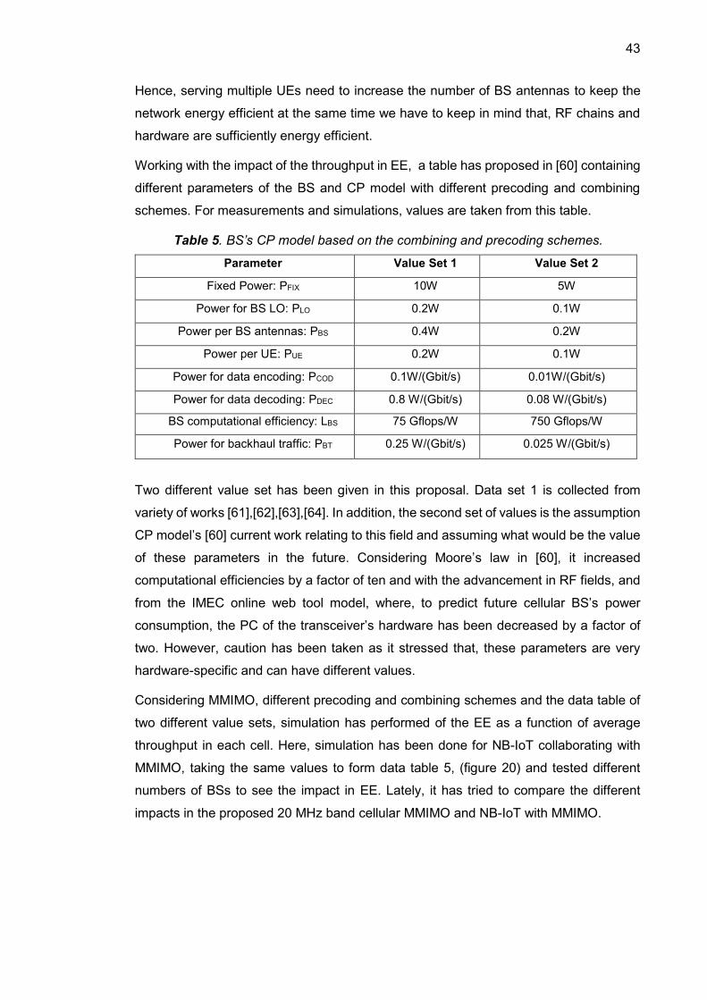
43
Hence, serving multiple UEs need to increase the number of BS antennas to keep the
network energy efficient at the same time we have to keep in mind that, RF chains and
hardware are sufficiently energy efficient.
Working with the impact of the throughput in EE, a table has proposed in [60] containing
different parameters of the BS and CP model with different precoding and combining
schemes. For measurements and simulations, values are taken from this table.
Table 5. BS’s CP model based on the combining and precoding schemes.
Parameter Value Set 1 Value Set 2
Fixed Power: PFIX 10W 5W
Power for BS LO: PLO 0.2W 0.1W
Power per BS antennas: PBS 0.4W 0.2W
Power per UE: PUE 0.2W 0.1W
Power for data encoding: PCOD 0.1W/(Gbit/s) 0.01W/(Gbit/s)
Power for data decoding: PDEC 0.8 W/(Gbit/s) 0.08 W/(Gbit/s)
BS computational efficiency: LBS 75 Gflops/W 750 Gflops/W
Power for backhaul traffic: PBT 0.25 W/(Gbit/s) 0.025 W/(Gbit/s)
Two different value set has been given in this proposal. Data set 1 is collected from
variety of works [61],[62],[63],[64]. In addition, the second set of values is the assumption
CP model’s [60] current work relating to this field and assuming what would be the value
of these parameters in the future. Considering Moore’s law in [60], it increased
computational efficiencies by a factor of ten and with the advancement in RF fields, and
from the IMEC online web tool model, where, to predict future cellular BS’s power
consumption, the PC of the transceiver’s hardware has been decreased by a factor of
two. However, caution has been taken as it stressed that, these parameters are very
hardware-specific and can have different values.
Considering MMIMO, different precoding and combining schemes and the data table of
two different value sets, simulation has performed of the EE as a function of average
throughput in each cell. Here, simulation has been done for NB-IoT collaborating with
MMIMO, taking the same values to form data table 5, (figure 20) and tested different
numbers of BSs to see the impact in EE. Lately, it has tried to compare the different
impacts in the proposed 20 MHz band cellular MMIMO and NB-IoT with MMIMO.

44
Figure 20. EE as a function of average throughput per cell for L = 16. Taking
into consideration of NB-IoT and the first set of the value-form table. M from 1o to 200 with a step size of 10 and K = 10. All combining and precoding schemes are increasing EE and throughput but M-MMSE has the highest
EE values followed by S-MMSE.
Figure 20 illustrates EE versus throughput for all schemes when the number of BSs is
16 and the number of BS antennas varies from 10 to 200 in step size of 10. EE becomes
and unimodal function of throughput for the value set 1 of the table for all schemes. It
means EE and throughput can jointly increase until the maximum edge of EE. After that,
EE falls at the cost of increasing throughput. From different schemes, the highest EE at
different throughput points is observed. M-MMSE has the highest EE for any value
regarding throughput followed by S-MMSE. Maximum M-MMSE for this setup is 0.227
Mbit/Joule/cell corresponding throughput of 6 Mbit/s/cell. Moreover, this maximum EE
is conquered at M = 30. Hence, the total area throughput stands for 96 Mbit/s/km2.
With S-MMSE, the highest EE obtained is 0.2136 Mbit/joule/cell which reduced EE by
6.3% compared to M-MMSE and corresponding throughput of 5.638 Mbit/s/cell which is
also lower than M-MMSE by 6.5%. Both achieved at M = 30.
RZF and ZF have almost similar performance except. RZF has maximal EE of 0.1985
Mbit/joule corresponding throughput of 5.24 Mbit/s/cell and it’s achieved when M = 30.
On the contrary, ZF has 0.195 Mbit/joule EE for throughput of 5.927 Mbit/s/cell and it
comes at M = 40.

45
MR provides maximal EE of 0.1043 Mbit/joule corresponding to the throughput of 3.17
Mbit/s/cell. Therefore, the total throughput of the area stands for 1.6688 Mbit/s/km2.
Now, if a comparison is made for the NB-IoT collaborating with MMIMO system with
defined cellular MMIMO, at first glance it seems like EE and throughput has been fallen
in NB-IoT compared to 20 MHz band MMIMO. But it doesn’t happen actually. Compare
taking the value of M-MMSE,
In [60], for M-MMSE scheme, 21.26 Mbit/joule/cell of EE is achieved considering the
throughput of 600 Mbit/s/cell and total area throughput of 9.6 Gbit/s/km2. In addition to
NB-IoT, it is 0.227 Mbit/joule/cell EE at the cost of 6.008 Mbit/s/cell throughput and total
area throughput of 96 Mbit/s/km2. In both cases, the highest EE is obtained at M = 30.
But, in 20 MHz band MMIMO, in [60] BW of 20 MHz is used and for NB-IoT BW is only
200 kHz, which is 100 times smaller. Now, if multiplication can be done with the EE and
throughput by the factor of 100, it can be obtained EE of 22.7 Mbit/joule/cell and each
cell throughput of 600 Mbit/s. Which stands total throughput of 9.6 Gbit/s/km2. Comparing
these two scenarios, a conclusion can be made like, with the same throughput and
number of antennas NB-IoT with MMIMO has better EE (approximately 6.3%) than
traditional 20 MHz Band MMIMO.
In the time following, to see the impact of increasing the number of BSs, the simulation
has done considering the same scenario. BS numbers are taken as, L = 32, L = 64, and
L = 128, 3 more different values to observe the changes in EE (figure 21, 22 and 23).
Figure 21. EE as a function of average throughput per cell for L = 32

46
Figure 22. EE as a function of average throughput per cell for L = 32
Figure 23. EE as a function of average throughput per cell for L = 64
From figures 21, 22, and 23, it can observe that increasing the BS number has no or
very little impact on both EE and throughput. This is due to the fact that the system has
calculated the EE versus throughput depending on the CP model, where consideration
is only in the PFIX, PBS, PUE, PLO, PCOD, PDEC & PBT. Now, in every case, the number of
transmitting antennas, M remained fixed (from 10 to 200 in steps of 10). Hence,
increasing L has either no or negligible impact on the EE versus throughput curve.

47
Figure 24. EE as a function of average throughput per cell for the NB-IoT with
MMIMO system. Considering hardware parameters from value set 2 and the number of BS, L = 16. Different throughputs are gained varying numbers to transmitter antenna, M from 20 to 200 with a step size of 10. Apart from the
Hardware parameter’s value set, rest are kept the same.
Taking the value set 2 from the table (where computational efficiencies have been
increased by a factor of ten and transceiver’s hardware PC has been decreased by a
factor of two) the simulation has done exactly the same as the value set 1 for NB-IoT
with MMIMO (figure 24). It is observed that, for all considered combining and precoding
schemes, the EE is almost double.
Comparing figure 20 (for the value set 1) with figure 24 (for the value set 2), EE has
become almost double due to reducing most of the coefficient of CP. The maximum EE
has achieved in the M-MMSE scheme among all the schemes followed by S-MMSE. In
M-MMSE, EE is 0.4224 Mbit/joule/cell followed by S-MMSE of 0.3947 Mbit/joule/cell.
Both are achieved for M = 40 and M = 30 respectively. Throughput per cell 6.88 Mbit/s
for M-MMSE and 5.638 Mbit/s for S-MMSE. For RZF and ZF schemes, the highest EE
is achieved at the cost of M = 40 and after M = 40, increasing throughput causes EE
decreasing. The downslope is almost similar for both schemes. It achieved 0.1947
Mbit/joule/cell EE for MR along with 3.17 Mbit/s/cell throughput. However, in both value
sets, the MR curve is smoother than with other schemes.
Again, comparing NB-IoT collaboration with MMIMO scheme and 20 MHz band defined
MMIMO scheme, the same output is observed. For MMIMO (B = 20 MHz), where for the
value Set 2, it has achieved EE 41.52 Mbit/Joule/cell corresponding throughput of 688
Mbit/s/cell. Whereas, for NB-IoT collaboration with MMIMO has obtained EE of 0.4224
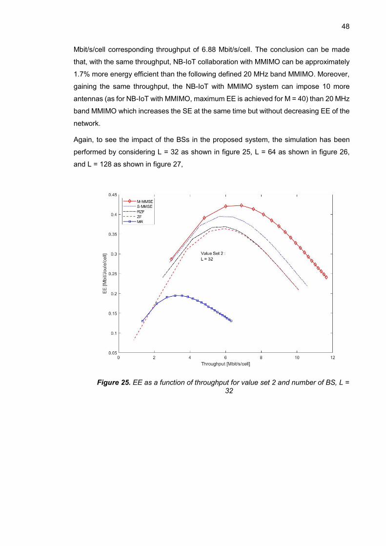
48
Mbit/s/cell corresponding throughput of 6.88 Mbit/s/cell. The conclusion can be made
that, with the same throughput, NB-IoT collaboration with MMIMO can be approximately
1.7% more energy efficient than the following defined 20 MHz band MMIMO. Moreover,
gaining the same throughput, the NB-IoT with MMIMO system can impose 10 more
antennas (as for NB-IoT with MMIMO, maximum EE is achieved for M = 40) than 20 MHz
band MMIMO which increases the SE at the same time but without decreasing EE of the
network.
Again, to see the impact of the BSs in the proposed system, the simulation has been
performed by considering L = 32 as shown in figure 25, L = 64 as shown in figure 26,
and L = 128 as shown in figure 27,
Figure 25. EE as a function of throughput for value set 2 and number of BS, L = 32

49
Figure 26. EE as a function of throughput for value set 2 and number of BS, L = 64
Figure 27. EE as a function of throughput for value set 2 and number of BS, L = 128
From figure 25, 26, and 27 as expected, there is no or very tiny (which can be negligible)
effect of L over EE.

50
To put it in a nutshell, the M-MMSE scheme has the best EE against throughput from
any other schemes. But the computational complexity is higher in this case, and for high
throughput, high CP is needed. Hence, CP is higher in this scheme compared to others.
A similar situation is observed in the case of S-MMSE. RZF and ZF have almost the
same EE across the same throughput. But for small throughput value, ZR deteriorates
abruptly.
To recapitulate, EE is a unimodal function of the throughput for both 20MHz band
MMIMO and NB-IoT with MMIMO scenarios. Maximum EE has achieved when M = 30
or M = 40 for different schemes serving for 10 UEs. NB-IoT with MMIMO has a better EE
scenario compared to 20 MHz band MMIMO for similar throughput. And EE reaches its
maximum edge when the antenna-UE ratio, M/K becomes 3 or 4 as we have obtained.
Simulation results show in figures 25 and 26 that with a fixed number of UEs, increasing
M up to 30 or 40 depending on schemes, EE has increased. However, if the number of
UEs is also increase at the same time, then the scenario becomes different from what is
obtained.
In this final step, a scratch network with modified parameters is observed to obtain the
highest EE with varying both antenna and UE. The perspective is to achieve the optimum
antenna-UE ratio without a priori assumptions so that our EE becomes highest.
In [60], achievable EE for MMIMO with different M/K values along with different
combination schemes have shown. In this thesis, simulation has been performed for NB-
IoT with MMIMO to observe the results and to come to the conclusion (figure 28).
To simulate this, the value set 1 has taken from table 5 except the number of UE which
is considered here from 10 up to 200 with a step size of 10 and the number of antennas
from 20 to 200 with the same step size.

51
Figure 28. Maximal EE as a function of M/K for the M-MMSE combining
scheme. Considering value set 1 from table 5.1 and K ∈ {10, 20, 30, . . .
200}, M ∈ {20, 30, 40, . . . 200} with a step size of 10 for both.
Figure 29. Maximal EE as a function of M/K for the RZF combining scheme.
Considering value set 1 from table 5.1 and K ∈ {10, 20, 30, . . . 200}, M ∈
{20, 30, 40, . . . 200} with a step size of 10 for both.

52
Figure 30. Maximal EE as a function of M/K for MR combining scheme. Considering value set 1 from table 5.1 and K ∈ {10, 20, 30, . . . 200}, M ∈
{20, 30, 40, . . . 200} with step size of 10 for both.
From figure 28, 29, 30 it is observed that, for NB-IoT with MMIMO in every combining
scheme, there is a global optimum EE point and the surface of the EE curve is concave.
It is obtained a different M/K ratio to achieve this global maximal EE. With M-MMSE
scheme, it has obtained the maximal EE of 0.2636 Mbit/Joule corresponding (M,K) =
(70,30) or M/K = 2.3~ 2.5. With RZF and MR schemes, we got EE of 0.2226 Mbit/Joule
at the cost of (M, K) = (90,30) or the ratio, M/K = 3. In addition to MR combining 0.1121
Mbit/Joule EE has acquired at the cost of (M, K) = (60,20) or the ratio of M/K = 3. A piece
of positive and important information can be acquired from here. That is, for M-MMSE,
the ratio for M and K is decreased. For, cellular MMIMO, the M/K is 3 to 4 whereas for
NB-IoT with MMIMO it is 2.3~2.5 which indicates that, to obtain the same SE NB-IoT
with MMIMO may need fewer antennas compared to the considered reference MMIMO
system. It means that energy can be saved more in NB-IoT with MMIMO than considered
reference MMIMO system as less number of antenna needs fewer RF chains, DAC,
ADC, I/Q mixers, PAs, and others part which consume power.
Here, experiments have performed under the consideration of M-MMSE, ZRF, and MR
combining scenarios because S-MMSE and ZF have almost similar CP to that of RZF.
From the simulation, it can be that EE is maximized when the antenna-UE ratio(M/K) is
between 2.5 to 3, and M-MMSE has the best performance with this ratio from the

53
perspective of EE and throughput. However, as it has already said that, due to larger M
and K values, CP increases in this scheme more. Moreover, computational complexity
is still present here. However, with more energy-efficient hardware and within our
resultant M/K = 2.5~3 ratio, M-MMSE is the potential solution for EE from the throughput
and SE perspective.
From all of these simulations and comparisons between NB-IoT with MMIMO and 20
MHz band cellular MMIMO technology to observe tradeoff EE and SE, the conclusion
can be made as,
1. Noise Power, 𝜎2 should be minimized or average channel gain of the active UE
should be increased at any cell so that the values of 𝜎2
𝛽 can be kept smaller. For this
circumstance, NB-IoT with MMIMO has better performance than that of 20 MHz band
cellular MMIMO. However, if the value of 𝜎2
𝛽 can be kept like -8 dBm or 9-dBm (usual
case it is -6 dBm), 20MHz cellular MMIMO EE performance against SE will be better.
2. The power consumption of BS transceiver hardware should be minimized by a factor
of 2 or at least 1.5 in order to get a better EE-SE tradeoff. With the advancement in
the field of RF and electronics, BS’s hardware technology already works on that [7]
to make some extent energy-efficient transceiver’s hardware.
3. For the best EE-SE tradeoff, the antenna-UE ratio or M/K should be in-between 3-4
and for NB-IoT with MMIMO it would be 2-3.
4. For this M/K ratio, M-MMSE can be better combining scheme for better EE-SE
tradeoff as well as for throughput if energy-efficient transceiver hardware can be
considered. Since M/K ratio is between 2 to 3 for NB-IoT with MMIMO and 3 to 4 for
20 MHz bands defined cellular MMIMO, computational complexity would be within a
reasonable range. In turn as an alternative option, RZF can be used which provides
moderate tradeoff.
54
6. CONCLUSION
In this thesis, a framework for EE-SE tradeoff is presented in the wireless communication
network using a simple two-cell Wyner model considering 4*4 cells and 0.25km*0.25km
per cell dimension. Improvisation has been done from [60] and attempts have been taken
to modify it for better EE-SE tradeoff. Besides, an effort has given to observe whether
the EE and SE will be upgraded or not if, in the future, NB-IoT will collaborate with
MMIMO. The simulations and results have proven that, if the ratio of signal’s noise power
and the average channel gain of active user equipments can be decreased, the EE-SE
tradeoff becomes better, as noise power-average channel gain ratio value decrease
which improves the EE-SE tradeoff. Besides, increasing the power amplifier’s efficiency
has the same result as expected. The best possible way to increase that is, firstly, to use
multiple PAs instead of a big powerful one, because the loss factor is higher in a bigger
one than a few smaller ones. Secondly, decreasing the cell radius. If the cell radius is
small, the signal need not be amplified more. Uses of power amplifiers will be limited and
hence loss factor will be decreased as well. In that scenario, NB-IoT with MMIMO would
show better performance compared to defined 20 MHz band cellular MMIMO. Choosing
precoding and combining schemes have a great impact on EE-SE tradeoff. MMSE has
the best performance in terms of EE-SE tradeoff. Though the computational complexity
is high, other schemes can’t transgress its barrier. Besides, with the consideration of
Moore’s law, the IMEC web tool model, and the advancement in the field of RF
technologies, computational complexity is becoming diminished [61]. Finally, when the
wireless network can be able to keep the antenna-user equipment ratio between 3-4, the
best EE-SE tradeoff can be achieved. In addition, in the future, considering Moore’s law,
if the power consumption of the transceiver’s hardware can decrease by a factor of two
and increase computational efficiencies by a factor of 10, both EE and SE will be
increased and resultant, better EE-SE tradeoff can be achieved than ever. Also, the
antenna-user equipment ratio will be lower.
However, fulfilling Moore’s law regarding BS’s circuit power consumption model is the
open challenge right now. Good thing is, researchers have already started working on
that [62]. Besides, they have also started working on efficient digital signal processing
and circuit architecture to minimize the CP consumption for MMIMO [63].
In the future, structure-based MMIMO alone with such a high increasing rate of the UEs
in wireless networks will not be able to provide the best throughput as its proving right
now. As the world is going through Internet-of-things, we must collaborate NB-IoT

55
technology with MMIMO networks. Although researchers have been trying to customize
MMIMO’s antennas to collaborate with both narrowband and ultrawide-band, emphasis
should be given more to make it happen at the earliest possible time.

56
REFERENCES
[1] E. Gustafsson, A. Jonsson. Always best connected. IEEE Wireless
Communications. 2003;10(1):49-55. doi: 10.1109/MWC.2003.1182111.
[2] T. L. Marzetta. Massive MIMO: An introduction. Bell Labs Technical Journal.
2015;20:11-22. doi: 10.15325/BLTJ.2015.2407793.
[3] J. G. Andrews, S. Buzzi, W. Choi, et al. What will 5G be? IEEE Journal on
Selected Areas in Communications. 2014;32(6):1065-1082. doi:
10.1109/JSAC.2014.2328098.
[4] T. L. Marzetta. Noncooperative cellular wireless with unlimited numbers of
base station antennas. IEEE Transactions on Wireless Communications.
2010;9(11):3590-3600. doi: 10.1109/TWC.2010.092810.091092
[5] E. Björnson, E. G. Larsson, T. L. Marzetta. Massive MIMO: Ten myths and one
critical question. IEEE Communications Magazine. 2016;54(2):114-123. doi:
10.1109/MCOM.2016.7402270.
[6] F. Boccardi, R. W. Heath, A. Lozano, T. L. Marzetta, P. Popovski. Five
disruptive technology directions for 5G. IEEE Communications Magazine.
2014;52(2):74-80. doi: 10.1109/MCOM.2014.6736746.
[7] D. Lister, "An operators view on green radio", presented at the Proc. IEEE Int.
Workshop on Green Communications, 2009.
[8] D. C. Kilper, G. Atkinson, S. K. Korotky, et al. Power trends in communication
networks. IEEE Journal of Selected Topics in Quantum Electronics.
2011;17(2):275-284. doi: 10.1109/JSTQE.2010.2074187
[9] "Summer net internal demand capacity resources and capacity margins 2012
actual 2013–2017 projected", Energy Information Administration: Official
Energy Statistics from the U.S. Government, May 2015.
[10] J. G. Andrews, S. Buzzi, W. Choi, S. V. Hanly, A. Lozano, A. C. K. Soong, J. C.
Zhang. What will 5G be? IEEE Journal on Selected Areas in Communications.
2014;32(6):1065-1082. doi: 10.1109/JSAC.2014.2328098.
[11] Y. Chen, S. Zhang, S. Xu, G. Y. Li. Fundamental trade-offs on green wireless
networks. IEEE Communications Magazine. 2011;49(6):30-37. doi:
10.1109/MCOM.2011.5783982.
[12] H. Q. Ngo, E. G. Larsson, T. L. Marzetta. Energy and spectral efficiency of very
large multiuser MIMO systems. IEEE Transactions on Communications.
2013;61(4):1436-1449. doi: 10.1109/TCOMM.2013.020413.110848.
57
[13] H. Yang, T. L. Marzetta. Performance of conjugate and zero-forcing
beamforming in large-scale antenna systems. IEEE Journal on Selected Areas
in Communications. 2013;31(2):172-179. doi: 10.1109/JSAC.2013.130206.
[14] E. Björnson, L. Sanguinetti, J. Hoydis, M. Debbah. Optimal design of energy-
efficient multi-user MIMO systems: Is massive MIMO the answer? IEEE
Transactions on Wireless Communications. 2015;14(6):3059-3075. doi:
10.1109/TWC.2015.2400437.
[15] W. Liu, S. Han, C. Yang, C. Sun. Massive MIMO or small cell network: Who is
more energy efficient?. 2013;24-29. doi: 10.1109/WCNCW.2013.6533309.
[16] C. Li, J. Zhang, K. B. Letaief. Throughput and energy efficiency analysis of
small cell networks with multi-antenna base stations. IEEE Transactions on
Wireless Communications. 2014;13(5):2505-2517. doi:
10.1109/TWC.2014.031714.131020.
[17] H. Li, L. Song, M. Debbah. Energy efficiency of large-scale multiple antenna
systems with transmit antenna selection. IEEE Transactions on
Communications. 2014;62(2):638-647. doi:
10.1109/TCOMM.2014.011414.130498.
[18] B. M. Lee, J. H. Choi and J. H. Bang, "An energy efficient antenna selection for
large scale green MIMO systems", Proc. IEEE Int. Symp. Circuits Syst., pp.
950-953, May. 2013.
[19] S. K. Goudos, M. Deruyck, D. Plets, et al. A novel design approach for 5G
massive MIMO and NB-IoT green networks using a hybrid jaya-differential
evolution algorithm. IEEE Access. 2019;7:105687-105700. doi:
10.1109/ACCESS.2019.2932042.
[20] J. Aquil, D. Sarkar, K. V. Srivastava. Eight-port MIMO antenna for integrated
narrowband / ultra-wideband (UWB) applications. 2018 IEEE Indian
Conference on Antennas and Propogation (InCAP). 2018:1-4. doi:
10.1109/INCAP.2018.8770754.
[21] G. Manganaro, D. Leenaerts, “Advances in Analog and RF IC Design for
Wireless Communication Systems”, 2013;1:1-6. doi: 10.1016/B978-0-12-
398326-8.00001-7. [Online].
Available:https://www.sciencedirect.com/science/article/pii/B978012398326800
0017.
[22] M. Alam, D. Yang, J. Rodriguez, R. A. Abd-alhameed. Secure device-to-device
communication in LTE-A. IEEE Communications Magazine. 2014;52(4):66-73.
doi: 10.1109/MCOM.2014.6807948.
[23] U. N. Kar, D. K. Sanyal. An overview of device-to-device communication in
cellular networks. 2018;4(4):203-208. doi: 10.1016/j.icte.2017.08.002. [Online].

58
Available:https://www.sciencedirect.com/science/article/pii/S240595951730146
7.
[24] M. Hicham, N. Abghour, M. Ouzzif. Device-To-Device (D2D) Communication
Under LTE-Advanced Networks. International Journal of Wireless & Mobile
Networks. 2016;8: 11-22. doi: 10.5121/ijwmn.2016.8102.
[25] S. Kinney. What is massive MIMO. Jun. 2017. [Online].
Available:https://www.rcrwireless.com/20170628/5g/what-is-massive-mimo-
tag17-tag99.
[26] E. G. Larsson, O. Edfors, F. Tufvesson, T. L. Marzetta. Massive MIMO for next
generation wireless systems. IEEE Communications Magazine.
2014;52(2):186-195. doi: 10.1109/MCOM.2014.6736761.
[27] J. Mundy, K. Thomas, What is massive MIMO technology? [Online]. Available:
https://5g.co.uk/guides/what-is-massive-mimo-technology/.
[28] R. Ratasuk, N. Mangalvedhe, A. Ghosh. Overview of LTE enhancements for
cellular IoT. 2015 IEEE 26th Annual International Symposium on Personal,
Indoor, and Mobile Radio Communications (PIMRC). 2015:2293-2297. doi:
10.1109/PIMRC.2015.7343680.
[29] D. Patel, M. Won. Experimental study on low power wide area networks for
mobile internet of things, in: Proc. of VTC, Sydney, Australia. 2017: 1-5
[30] M. Centenaro, L. Vangelista, A. Zanella, M. Zorzi. Long-range communications
in unlicensed bands: The rising stars in the IoT and smart city scenarios. IEEE
Wireless Communications. 2016;23(5):60-67. doi:
10.1109/MWC.2016.7721743.
[31] Spectral efficiency, En.wikipedia.org, 2019. [Online]. Available:
https://en.wikipedia.org/wiki/Spectral_efficiency. [Accessed: 17- Oct- 2019].
[32] R. Hranac. Spectral Efficiency. Scte.org, 2019. [Online]. Available:
https://www.scte.org/TechnicalColumns/12-10-
01%20spectral%20effieciency.pdf. [Accessed: 17- Oct- 2019].
[33] T. Cheng, A. Keintola. Why Does Spectral Efficiency Matter?,
Bluedanube.com, 2019. [Online]. Available:
https://www.bluedanube.com/blog/2018/07/23/why-does-spectral-efficiency-
matter/. [Accessed: 17- Oct- 2019]
[34] A. Zappone, E. Jorswieck. Energy efficiency in wireless networks via fractional
programming theory. Foundations and Trends in Communications and
Information Theory. 2015;11(3-4):185–396. doi: 10.1561/0100000088.
59
[35] M. Rouse. What is throughput? - Definition from
WhatIs.com, SearchNetworking, 2019. [Online]. Available:
https://searchnetworking.techtarget.com/definition/throughput. [Accessed: 17-
Oct- 2019].
[36] Power consumption, Wikipedia, 2019. [Online]. Available:
https://simple.wikipedia.org/wiki/Power_consumption#cite_not. [Accessed: 17-
Oct- 2019].
[37] E. Björnson, J. Hoydis, L. Sanguinetti. Massive MIMO Networks: Spectral,
Energy, and Hardware Efficiency, Foundations and Trends® in Signal
Processing: 2017;11(3-4):154-655. doi: 10.1561/2000000093. [Online].
Available: https://ieeexplore.ieee.org/servlet/opac?bknumber=8187178.
[38] Z. Hasan, H. Boostanimehr, V. K. Bhargava. Green cellular networks: A
survey, some research issues and challenges. IEEE Communications Surveys
& Tutorials. 2011;13(4):524-540. doi: 10.1109/SURV.2011.092311.00031.
[39] A. Ashikhmin, T. Marzetta. Pilot contamination precoding in multi-cell large
scale antenna systems. 2012 IEEE International Symposium on Information
Theory Proceedings. 2012:1137-1141. doi: 10.1109/ISIT.2012.6283031.
[40] G. Auer, O. Blume, V. Giannini. Energy efficiency analysis of the reference
systems, areas of improvements and target breakdown. 2010; 1-68.
[41] E. Björnson, J. Hoydis, L. Sanguinetti. Massive MIMO Networks: Spectral,
Energy, and Hardware Efficiency, Foundations and Trends® in Signal
Processing: 2017;11(3-4):154-655. doi: 10.1561/2000000093. [Online].
Available: https://ieeexplore.ieee.org/servlet/opac?bknumber=8187178
[42] E. Björnson, J. Hoydis, L. Sanguinetti. Massive MIMO Networks: Spectral,
Energy, and Hardware Efficiency, Foundations and Trends® in Signal
Processing: 2017;11(3-4):154-655. doi: 10.1561/2000000093. [Online].
Available: https://ieeexplore.ieee.org/servlet/opac?bknumber=8187178
[43] H. Yang, T. L. Marzetta. Total energy efficiency of cellular large scale antenna
system multiple access mobile networks. 2013 IEEE Online Conference on
Green Communications (OnlineGreenComm). 2013:27-32. doi:
10.1109/OnlineGreenCom.2013.6731024
[44] E. Björnson, L. Sanguinetti, J. Hoydis, M. Debbah. “Designing multi-user MIMO
for energy efficiency: When is massive MIMO the answer?” In: Proc. IEEE
WCNC. 2014; 242–247.
[45] E. Bjornson E, Sanguinetti L, Hoydis J, Debbah M. Optimal design of energy-
efficient multi-user MIMO systems: Is massive MIMO the answer? TWC.
2015;14(6):3059-3075. https://ieeexplore.ieee.org/document/7031971. doi:
10.1109/TWC.2015.2400437

60
[46] E. Björnson, L. Sanguinetti, M. Kountouris. Deploying dense networks for
maximal energy efficiency: Small cells meet massive MIMO. IEEE Journal on
Selected Areas in Communications. 2016;34(4):832-847. doi:
10.1109/JSAC.2016.2544498
[47] E. Björnson, J. Hoydis, L. Sanguinetti. Massive MIMO Networks: Spectral,
Energy, and Hardware Efficiency, Foundations and Trends® in Signal
Processing: 2017;11(3-4):154-655. doi: 10.1561/2000000093. [Online].
Available: https://ieeexplore.ieee.org/servlet/opac?bknumber=8187178
[48] E. Björnson, J. Hoydis, L. Sanguinetti. Massive MIMO Networks: Spectral,
Energy, and Hardware Efficiency, Foundations and Trends® in Signal
Processing: 2017;11(3-4):154-655. doi: 10.1561/2000000093. [Online].
Available: https://ieeexplore.ieee.org/servlet/opac?bknumber=8187178
[49] E. Björnson, J. Hoydis, L. Sanguinetti. Massive MIMO Networks: Spectral,
Energy, and Hardware Efficiency, Foundations and Trends® in Signal
Processing: 2017;11(3-4):154-655. doi: 10.1561/2000000093. [Online].
Available: https://ieeexplore.ieee.org/servlet/opac?bknumber=8187178
[50] E. Björnson, J. Hoydis, L. Sanguinetti. Massive MIMO Networks: Spectral,
Energy, and Hardware Efficiency, Foundations and Trends® in Signal
Processing: 2017;11(3-4):154-655. doi: 10.1561/2000000093. [Online].
Available: https://ieeexplore.ieee.org/servlet/opac?bknumber=8187178
[51] "Uplink Power Budget", Trepo.tuni.fi, 2019. [Online]. Available:
https://trepo.tuni.fi/bitstream/handle/123456789/27158/Kavuri.pdf?sequence=4
&isAllowed=y. pp 32. [Accessed: 17- Oct- 2019].
[52] Itu.int, 2019. [Online]. Available: https://www.itu.int/en/ITU-D/Regional-
Presence/AsiaPacific/SiteAssets/Pages/ITU-ASP-CoE-Training-on-
/Session5_NB_IoT%20networks%20web.pdf. [Accessed: 17- Oct- 2019].
[53] E. Björnson, J. Hoydis, L. Sanguinetti. Massive MIMO Networks: Spectral,
Energy, and Hardware Efficiency, Foundations and Trends® in Signal
Processing: 2017;11(3-4):154-655. doi: 10.1561/2000000093. [Online].
Available: https://ieeexplore.ieee.org/servlet/opac?bknumber=8187178
[54] E. Björnson, J. Hoydis, L. Sanguinetti. Massive MIMO Networks: Spectral,
Energy, and Hardware Efficiency, Foundations and Trends® in Signal
Processing: 2017;11(3-4):154-655. doi: 10.1561/2000000093. [Online].
Available: https://ieeexplore.ieee.org/servlet/opac?bknumber=8187178
[55] G. Castignani, J. Monetti, N. Montavont, A. A. Moret, R. Frank, T. Engel. A
study of urban IEEE 802.11 hotspot networks: Towards a community access
network. 2013 IFIP Wireless Days (WD). 2013:1-8. doi:
10.1109/WD.2013.6686459.

61
[56] I. Ashraf, F. Boccardi, L. Ho. SLEEP mode techniques for small cell
deployments. IEEE Communications Magazine. 2011;49(8):72-79. doi:
10.1109/MCOM.2011.5978418.
[57] J. Wu, Y. Zhang, M. Zukerman, E. K. Yung. Energy-efficient base-stations
sleep-mode techniques in green cellular networks: A survey. IEEE
Communications Surveys & Tutorials. 2015;17(2):803-826. doi:
10.1109/COMST.2015.2403395
[58] Evolved Universal Terrestrial Radio Access (E-UTRA); Radio frequency (RF)
system scenarios (Release 8). 2008. 3GPP TS 36.942
[59] R. Zi, X. Ge, J. Thompson, C. Wang, H. Wang, T. Han. Energy efficiency
optimization of 5G radio frequency chain systems. IEEE Journal on Selected
Areas in Communications. 2016;34(4):758-771. doi:
10.1109/JSAC.2016.2544579.
[60] E. Björnson, J. Hoydis, L. Sanguinetti. Massive MIMO Networks: Spectral,
Energy, and Hardware Efficiency, Foundations and Trends® in Signal
Processing: 2017;11(3-4):154-655. doi: 10.1561/2000000093. [Online].
Available: https://ieeexplore.ieee.org/servlet/opac?bknumber=8187178
[61] S. Ahmed, F. Iqbal, S. Kim. Complexity reduction of MMSE method for iterative
MIMO systems. 2018 International Conference on Information and
Communication Technology Convergence (ICTC). 2018:10-14. doi:
10.1109/ICTC.2018.8539477.
[62] T. A. Khan, A. Yazdan, Y. Maguire, R. W. Heath. Energy efficiency of wireless
information and power transfer with massive MIMO. 2017 IEEE 85th Vehicular
Technology Conference (VTC Spring). 2017:1-5. doi:
10.1109/VTCSpring.2017.8108320.
[63] L. Van der Perre, L. Liu, E. G. Larsson. Efficient DSP and circuit architectures
for massive MIMO: State of the art and future directions. IEEE Transactions on
Signal Processing. 2018;66(18):4717-4736. doi: 10.1109/TSP.2018.2858190.
[64] "Power Model for Wireless Base Stations", Imec-int.com, 2019. [Online].
Available: https://www.imec-int.com/en/powermodel. [Accessed: 21- Oct-
2019].
[65] X. Gao, O. Edfors, F. Rusek, F. Tufvesson. Massive MIMO performance
evaluation based on measured propagation data. IEEE Transactions on
Wireless Communications. 2015;14(7):3899-3911. doi:
10.1109/TWC.2015.2414413
[66] Data Structures - Asymptotic Analysis - Tutorialspoint, Tutorialspoint.com,
2019. [Online]. Available:
62
https://www.tutorialspoint.com/data_structures_algorithms/asymptotic_analysis
.htm. [Accessed: 28- Oct- 2019].
[67] J. Hoydis, S. T. Brink, M. Debbah. Massive MIMO in the UL/DL of cellular
networks: How many antennas do we need? J-SAC. 2013;31(2):160-
171. https://ieeexplore.ieee.org/document/6415388. doi:
10.1109/JSAC.2013.130205
[68] T. L. Marzetta. Noncooperative cellular wireless with unlimited numbers of
base station antennas. IEEE Transactions on Wireless Communications.
2010;9(11):3590-3600. doi: 10.1109/TWC.2010.092810.091092
[69] F. Rusek, D. Persson, B. K. Lau, et al. Scaling up MIMO: Opportunities and
challenges with very large arrays. IEEE Signal Processing Magazine.
2013;30(1):40-60. doi: 10.1109/MSP.2011.2178495
[70] S. Misra. Millimeter wave wireless communications (rappaport, T., et al; 2014)
[book review]. IEEE Wireless Communications. 2015;22(5):6-7. doi:
10.1109/MWC.2015.7306370.
[71] X. Li, E. Björnson, E. G. Larsson, S. Zhou, J. Wang. Massive MIMO with multi-
cell MMSE processing: exploiting all pilots for interference suppression.
https://jwcn-eurasipjournals.springeropen.com/articles/10.1186/s13638-017-
0879-2. Published 2019. Accessed October 28, 2019.
[72] E. Björnson, J. Hoydis, L. Sanguinetti. Massive MIMO Networks: Spectral,
Energy, and Hardware Efficiency, Foundations and Trends® in Signal
Processing: 2017;11(3-4):154-655. doi: 10.1561/2000000093. [Online].
Available: https://ieeexplore.ieee.org/servlet/opac?bknumber=8187178
[73] D. Malik, D. Batra. Comparison of various detection algorithms in a MIMO
wireless communication receiver. Pdfs.semanticscholar.org.
https://pdfs.semanticscholar.org/0b6c/a18db525b9669876c97e0180a45ae5a9
9cbe.pdf. Published 2019. Accessed October 28, 2019.
[74] Lambert W-Function -- from Wolfram MathWorld. Mathworld.wolfram.com.
http://mathworld.wolfram.com/LambertW-Function.html. Published 2019.
Accessed November 3, 2019.
[75] Euler Number -- from Wolfram MathWorld.
Mathworld.wolfram.com.http://mathworld.wolfram.com/EulerNumber.html.
Published 2019. Accessed November 3, 2019.
[76] R. V. Raja Kumar, J. Gurugubelli. How green the LTE technology can be?.
Semanticscholar.org. https://www.semanticscholar.org/paper/How-green-the-
LTE-technology-can-be-Kumar
Gurugubelli/10248d17ede7b6186971a941a6afd2e01f684282. Published 2011.
Accessed November 13, 2019.

63
[77] G. Auer,O. Blume, V. Giannini, I. Godor, M. A. Imran, Y. Jading, E. Katranaras,
M. Olsson, D. Sabella, P. Skillermark, and W. Wajda. 2012. D2.3: Energy
efficiency analysis of the reference systems, areas of improvements and target
breakdown. INFSOICT – 247733 EARTH, ver. 2.0.
![Spectral Efficiency and Energy Efficiency in Massive MIMO ...wingn/Diwei_Sun_thesis.pdf · (P2P) system [12], spectral efficiency in massive MIMO systems are enhanced significantly,](https://img.dokumen.tips/doc/110x75/5f0382b97e708231d4096b34/spectral-efficiency-and-energy-efficiency-in-massive-mimo-wingndiweisun-.jpg)


![Distributed Spectral Efficiency Optimization At Hotspots ... · Distributed Spectral Efficiency Optimization At ... the QoS and system wide throughput in WCS. ... HSDPA [6] and LTE](https://img.dokumen.tips/doc/110x75/5b1906037f8b9a3c258c4bb6/distributed-spectral-efficiency-optimization-at-hotspots-distributed-spectral.jpg)