Embed Size (px)
Citation preview

Modelling Alternative Generation’s Ability to Match Demand During Extreme Weather Events
E21 Conference Melbourne 2009
Presentation outline
1. Problem – timing difference between peak demand vs solar & wind generation
2. Peak demand trends over a day and a season
3. Supply trends over a day and a season
4. Simulating the seasonal trends of demand vs supply
5. Supply changes to offset the weather driven demand changes
6. Impact of extreme seasons
7. Conclusions
Background perspective
My background– Developing peak MW demand forecasting models
My perspective– Apparent lack of focus on how extreme weather events affect both
demand and supply (solar & wind) – as long term forecasting for each tends to be carried out separately
Aim– Simulate demand and supply in one model to demonstrate the
systematic shifts that occur in the balance over a typical and an extreme season
Benefit– A better understanding of how events, like extreme weather, can
impact on both demand and supply will facilitate a better the match between demand and solar & wind generators – lowering the redundancy in other types of generation to meet demand
Background perspective
Incorporating solar and wind generators into a network is an area of many complexities. To have a manageable project, I did not look at the following areas:
– calculating how many solar and wind generators will be required– the economics of alternative generation– the quality of the power supplied– feed-in tariffs & other incentives programs– the efficiency of different types of alternative generators– the size of the generators required to meet a distribution network’s
peak MW demand– the benefits of distributed generation on infrastructure investments– total energy supplied over a year
Firstly - what is demand
Customer demand is driven by all the factors you may expect including…– temperature, wind, rain, cloud cover, etc. affecting the air conditioning or
heating load– economic/population growth, appliance penetration/size/efficiency affecting
the growth over time
… as well as other more “social convention” type factors like:– time of the day, day of week, and weekends– Jan 30 and back to school, Xmas and other holidays – Hot Friday afternoons in industrial areas –
Peak MW demand the maximum rate (i.e. over 30 mins) of supply over a day, season, year etc.. And is the result of each of these factors interacting
Any model which matches demand against supply, needs to account for the combined impact of weather and in social convention type factors
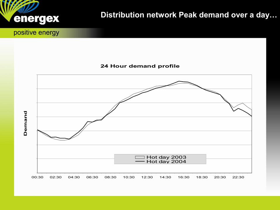
Distribution network Peak demand over a day…
24 Hour demand profile
00:30 02:30 04:30 06:30 08:30 10:30 12:30 14:30 16:30 18:30 20:30 22:30
Dem
an
d M
W
Hot day 2003Hot day 2004

…And over a season
• Every day as a profile from October to March
• Long axis on LHS – day of year. Short axis RHS – daily half hour intervals
• Chart is summer weekday data – as demand tends to be higher
• Different times of the year have different characteristics. i.e. October’s twin peaked profile vs’ February’s single
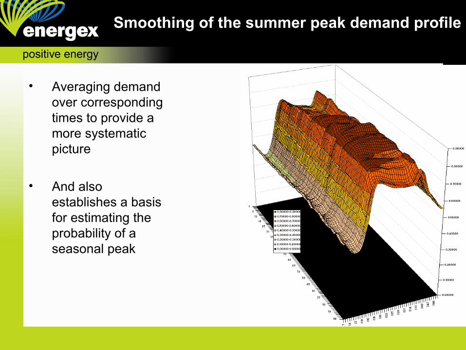
Smoothing of the summer peak demand profile
• Averaging demand over corresponding times to provide a more systematic picture
• And also establishes a basis for estimating the probability of a seasonal peak
Charts are based on index values
Index values– All the charts are based on index values. Each point is that half
hour’s demand relative to its season’s peak
Averaging over years– The use of an index enables multiple years of data to be added
together – without being corrupted by growth. It also enables supply to be subtracted from demand more easily
Use of available energy– Without actual solar and wind generation data, weather data was
used to create indexes based on ‘available’ energy. While this may not fully replicate the actual performance of the generators – it provides an good overall picture of systematic changes
Solar - solar radiation interval data from University of Queensland
Wind - wind speed interval data from University of Queensland

Building the supply side model
Generation types– solar and wind, both are influenced by the same weather
events as peak demand
Solar– hot sunny days are significant peak demand events and should
correspond with high output from solar generators
Wind– chosen because of its different generation characteristics to
solar (possible generation at night) and because of the potential for heatwaves to impact on the strength of the ambient wind
Modelling the supply side
Equal index values– solar and wind generation was modelled using the index based
approach as demand, avoiding the need to estimate the scale of the generation plant required to match demand
Index weightings– the relative contribution of solar or wind was changed with different
weightings applied to their index values
Negative index numbers– the supply side is differentiated by the use of negative index numbers,
to demonstrate the ‘imbalance’ between the demand and the supply
More volatile index values– solar and wind generation is far more volatile than demand, as this
type of generation has times of “zero” supply, while demand is always positive
Solar Supply index over a season
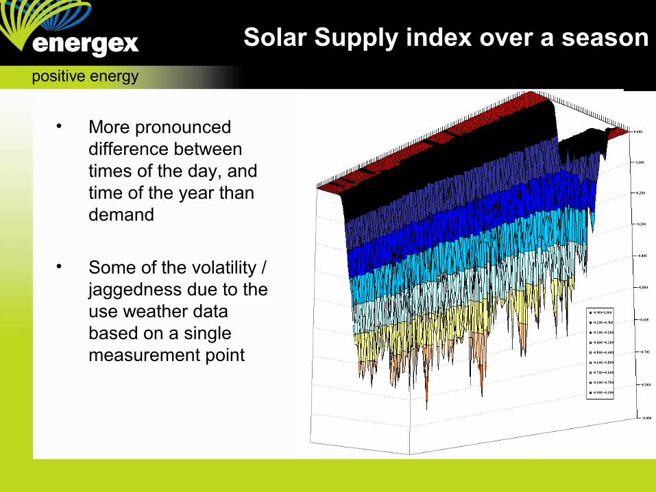
• More pronounced difference between times of the day, and time of the year than demand
• Some of the volatility / jaggedness due to the use weather data based on a single measurement point

Smoothing the index over corresponding times
Averaging supply over a corresponding times to provide a more systematic picture
Consistently high during the middle of the day for early in the summer, but seems to have a structural shift down later in the season, possibly changing solar angle/increased cloud cover?
Subtracting solar supply from demand
Balance, the net result– The balance between supply and demand is the net result of
each time interval’s ‘supply’ number is added to its ‘demand’ number
Lowering redundancy– The better that the wind and solar generators match
demand, the less reliance on other generators
The perfect outcome– Variations in demand to be perfectly met by solar & wind
generation supply. In a chart, this would appear as a flat plane – centred exactly at the zero index value
Balance: Solar v peak MW
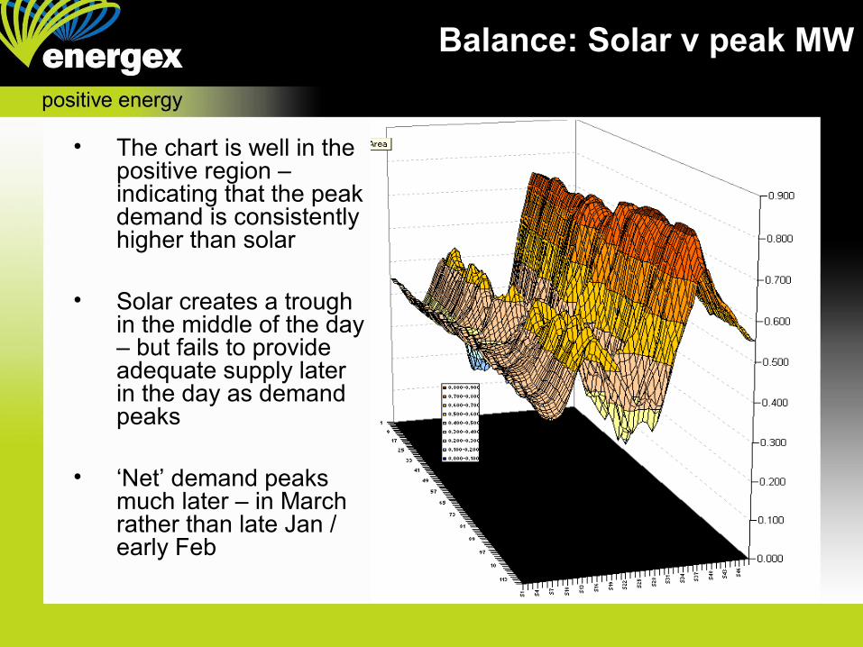
• The chart is well in the positive region – indicating that the peak demand is consistently higher than solar
• Solar creates a trough in the middle of the day – but fails to provide adequate supply later in the day as demand peaks
• ‘Net’ demand peaks much later – in March rather than late Jan / early Feb

Wind generation
• Now, taking a look at the contribution from wind generators.
• Once again, quite jagged compared to the demand index.
• Like solar, some of the volatility / jaggedness due to the use weather data based on a single measurement point
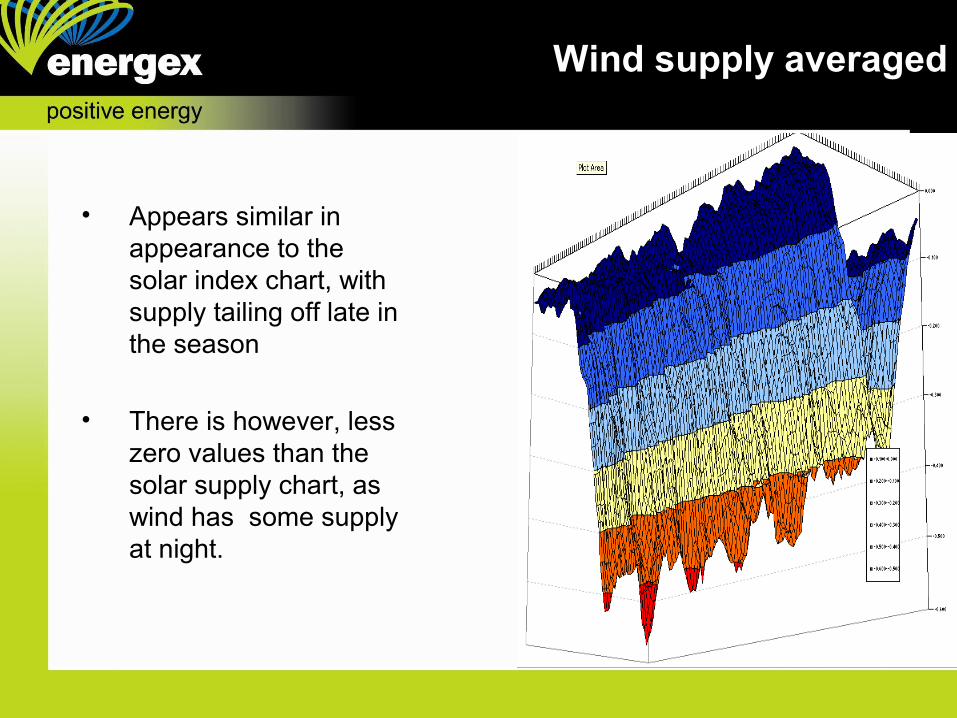
Wind supply averaged
• Appears similar in appearance to the solar index chart, with supply tailing off late in the season
• There is however, less zero values than the solar supply chart, as wind has some supply at night.
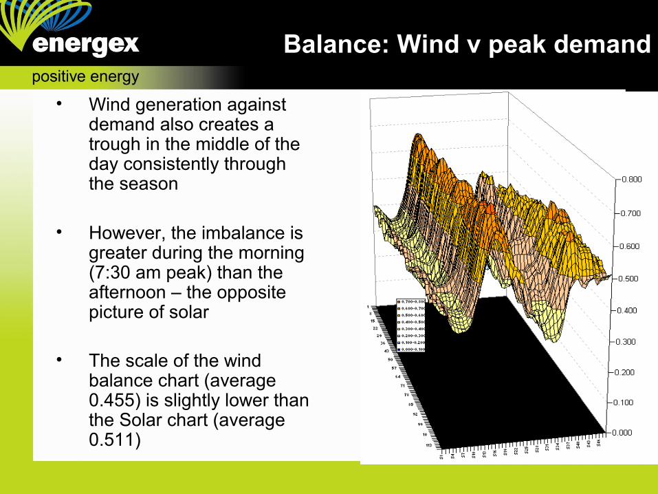
Balance: Wind v peak demand
• Wind generation against demand also creates a trough in the middle of the day consistently through the season
• However, the imbalance is greater during the morning (7:30 am peak) than the afternoon – the opposite picture of solar
• The scale of the wind balance chart (average 0.455) is slightly lower than the Solar chart (average 0.511)
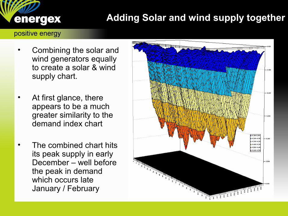
Adding Solar and wind supply together
• Combining the solar and wind generators equally to create a solar & wind supply chart.
• At first glance, there appears to be a much greater similarity to the demand index chart
• The combined chart hits its peak supply in early December – well before the peak in demand which occurs late January / February

Wind and solar supply against peak demand
• Solar and wind supply chart still has the characteristic peaks in morning and afternoon
• However, the peaks appear to be more evenly matched than the solar or wind supply charts alone.
• The time of the net demand peak has also been pushed back into late February, and the time from around 3pm to 7pm
Locating a solar plant
Solar plant location– To enable solar to more effectively offset demand, a theoretical exercise was
undertaken to “move” the solar generation plant to a location far from where demand is centred
Losses vs coincidence– While locating the plant away from the point of demand will result in higher
losses transporting the power back, it enables the solar plant to hit its maximum efficiency at the time when demand is peaking
New Zealand?– Initially the plant was chosen to be two hours east (NZ) and 2 hours west
(South/Western Australia), however this 2 hour offset was inadequate
Four hour time shift– A four hour shift was required to ‘flatten’ the solar supply profile enough to
make it correspond with the demand profile
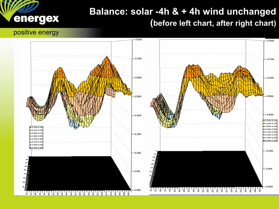
Balance: solar -4h & + 4h wind unchanged(before left chart, after right chart)
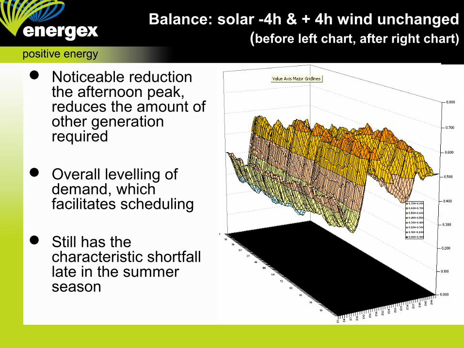
Balance: solar -4h & + 4h wind unchanged(before left chart, after right chart)
Noticeable reduction the afternoon peak, reduces the amount of other generation required
Overall levelling of demand, which facilitates scheduling
Still has the characteristic shortfall late in the summer season
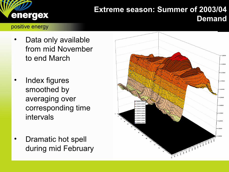
Extreme season: Summer of 2003/04Demand
• Data only available from mid November to end March
• Index figures smoothed by averaging over corresponding time intervals
• Dramatic hot spell during mid February
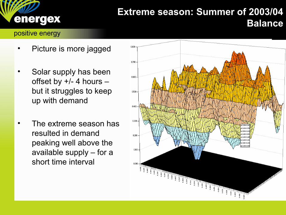
Extreme season: Summer of 2003/04Balance
• Picture is more jagged
• Solar supply has been offset by +/- 4 hours – but it struggles to keep up with demand
• The extreme season has resulted in demand peaking well above the available supply – for a short time interval

Extreme season: Summer of 2003/04Demand management 10% at peak
• To remove the spike in the imbalance between demand and supply, demand management initiatives are examined
• The DM simulation took the form of a 10% reduction in demand for 170 half hour intervals (3% of the total) for the year of 2004
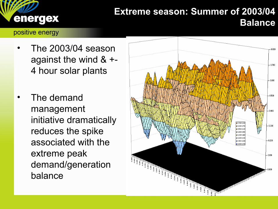
Extreme season: Summer of 2003/04Balance
• The 2003/04 season against the wind & +- 4 hour solar plants
• The demand management initiative dramatically reduces the spike associated with the extreme peak demand/generation balance
Limitations
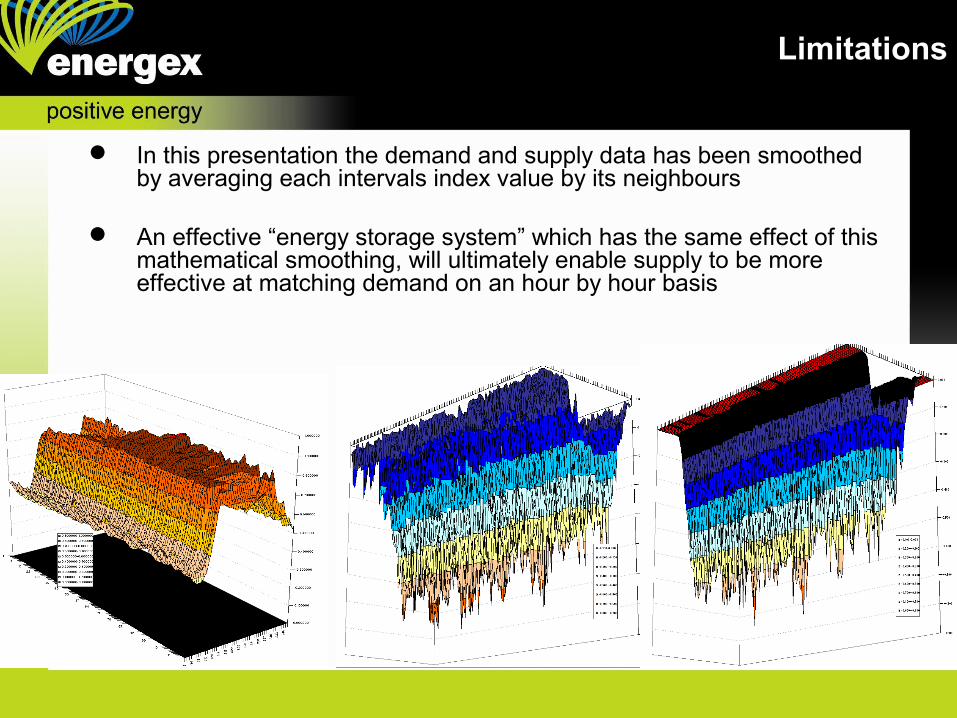
In this presentation the demand and supply data has been smoothed by averaging each intervals index value by its neighbours
An effective “energy storage system” which has the same effect of this mathematical smoothing, will ultimately enable supply to be more effective at matching demand on an hour by hour basis
Points to consider
Supply volatility– The contribution of solar and wind generators would greatly
increase if efficient storage systems were able to smooth supply shortfalls in the very short term (minute by minute) and in the long term for extreme seasons
Use of system costs – Total generation in the future may become more fragmented if
solar and wind generators remain proportionally smaller than current systems. This will require a corresponding increase in the transmission/distribution network to connect them to the grid
Transport costs– While integrating solar and wind generators across vast areas
enables use of the existing transmission/distribution network, it increases losses and other transport costs
Conclusions
Geographically distributed generation– A distributed network of solar plants enables wind and solar generation
to be matched more effectively against peak demand
Energy storage to smooth supply– Any incorporation of solar and wind generators will benefit substantially
from a good energy storage system to smooth out the short term volatility in supply
Extreme seasons a significant obstacle– Extreme weather events will require different strategies to those used
in average seasons, strategies which include factors like demand management
Simultaneous equations– This method of analysis also presents the possibility of using
simultaneous equations to determine the scale and mix of generators required by running scenarios

Questions, Comments, Contacts
Any questions? Comments?
Craig Pollard
Senior Forecasting Analyst
Energex
Ph 07 3407 4851
Mobile 0419 606 972