Embed Size (px)
Citation preview
ENERGETIC CARRYING CAPACITY OF HABITATS USED BY SPRING-
MIGRATING WATERFOWL IN THE UPPER MISSISSIPPI RIVER AND GREAT
LAKES REGION
A Thesis
Presented in Partial Fulfillment of the Requirements for
the Degree Master of Science in the
Graduate School of The Ohio State University
By
Jacob N. Straub, B.S.
*****
The Ohio State University 2008
Masters Examination Committee: Approved by Dr. Robert J. Gates, Adviser Dr. Tina Yerkes _______________________ Adviser Dr. Craig Davis Graduate Program in Natural Resources Dr. Stan Gehrt

ii
ABSTRACT
The Upper Mississippi River and Great Lakes region (UMRGLR), including
Wisconsin, Illinois, Indiana, Ohio, and Michigan, are part of an important migration
corridor for >12 million waterfowl annually. Waterfowl rely on wetland and cropland
habitats in the region to secure nutrients needed to complete life-history events. Wetland
loss in some of these states exceeds 95% of historic levels, raising concern that food
resources may be insufficient to support spring-migrating waterfowl. The goal of this
project was to improve understanding of food resource density and energy availability in
wetlands and adjacent cropland habitats used by spring-migrating waterfowl in the
UMRGLR. I collected plant and invertebrate food samples during two periods in spring
2006 in three wetland habitat classes (palustrine emergent, palustrine forested,
lacustrine/riverine) and croplands (corn and soybean) at six study areas in the UMRGLR.
I used two methods to convert food abundance to energetic carrying capacity (ECC)
estimates (duck use days/ha [dud/ha] ). The first method assumes constant food, habitat,
and daily energy requirements (ECCu), while the second uses foraging guild- (i.e., small
dabbling, grazing dabbling, omnivorous dabbling, and diving duck) specific food habits
and energy requirements (ECCw). Total estimated food biomass in wetlands consisted
almost entirely (>98%) of seeds, tubers, and invertebrates from benthic (substrate)
samples. I failed to detect a statistically significant difference between ECCu and ECCw
in 15 of 21 paired-t-test comparisons. The largest difference occurred in

iii
lacustrine/riverine wetlands in east-central Wisconsin where ECCu (59 dud/ha) was 88%
below ECCw (482 dud/ha). ECCw varied among study sites (F5,504 = 14.46, P<0.001),
and habitat types (F2,504 = 47.67, P<0.001) but did not differ by sampling period (F1,504 =
0.46, P = 0.500). ECCw was consistently greatest in palustrine emergent habitats (range
across sites = 613 – 1,287 dud/ha), and least in lacustrine habitats (range across sites = 22
– 342 dud/ha). Cropland ECC was more variable than in wetland habitats (ranges across
sites = 146- 3,303 dud/ha). Croplands had sufficient food energy to support large
numbers of waterfowl but few species are capable of foraging in this habitat.
Invertebrates did not contribute substantially to total food biomass or ECC for most sites
and habitat types. My estimates of ECC were below what the UMRGLR Joint Venture
assumes habitats provide. The greatest difference was in lacustrine habits where site-
specific habitat estimates were 82-99% lower than the Joint Venture estimate. Thus,
waterfowl that use lacustrine / deep water habitats may be energy-limited during spring
migration in the UMRGLR. My study examined the extent to which habitats used by
spring-migrating waterfowl in the UMRGLR can provide food energy abundance.
Conservation planners need reliable food abundance estimates for croplands, marshes,
natural lakes, rivers, impoundments, and riparian forests that individually and collectively
contribute to the total habitat resource that supports spring-migrating in the UMRGLR.
My results provide a basis for understanding variation in food resource abundance along
latitudinal and longitudinal gradients in the region and can strengthen the biological
foundation of strategic planning of habitat conservation to achieve population goals of the
North American Waterfowl Management Plan.

iv
ACKNOWLEDGMENTS Principle funding for this project was provided by the Ducks Unlimited Inc. Great
Lakes Atlantic Regional Office. Additional funding was provided by the U.S. Fish and
Wildlife Service Upper Mississippi Great Lakes Joint Venture, Ohio Department of
Natural Resources Division of Wildlife, Winous Point Marsh Conservancy, Ohio
Agriculture Research and Development Center, The Ohio State University School of
Environment and Natural Resources, Illinois Department of Natural Resources, Illinois
Natural History Survey, Wisconsin Department of Natural Resources, Waterfowl
Research Foundation, Saginaw Bay Watershed Initiative Network (WIN), Bruning
Foundation, Cristel DeHaan Family Foundation, DOW and Gerstocker Foundations.
I wish to thank Tina Yerkes, Craig Davis and Stan Gehrt for serving on my
committee. Tina has been instrumental in many aspects of my project and encouraged
me to pursue a master’s degree while I was working with DU in Michigan. I wish to
thank John Coluccy for review of my thesis draft as well as advice and assistance with
project planning. I also would like to express my gratefulness to Bob Gates for serving
as my graduate adviser. Bob provided motivation and support when I most needed it and
his confidence in my abilities allowed me to truly demonstrate my potential as a student
and researcher. I look forward to working with Bob in the future. In addition, I have
enjoyed having Bob as a friend, as it was always nice having another “cheesehead”
around.
v
I am indebted to Bill and Vivian Young as well as Elmer and Eleanor Naffein for
allowing myself and my field crew to use their accommodations at Marbill Island in
Michigan. I truly enjoyed my time spent with them and Elmer’s “home-made” wine.
The accommodations were far more than any graduate student could ever ask for. My
experiences and memories on one of the last remaining Great Lakes coastal wetlands will
always be cherished.
I wish to express my gratitude to all the individuals who helped with the
development and execution of this project. I extend a great thanks to all the field
technicians who helped on this project, especially Alan Leach, Ron Sting, and Matt
Schroeder, although I’m still not sure if they liked working with me or simply liked the
fact they could legally shoot ducks in the spring. I must also acknowledge all the hard
work of the “seed” technicians including, Casey Wright, Mariah Linkhart, Chriss Grimm,
Carly Kestler, Dustin Kasier, and Gretchen Walburn have put forth. They have put in
countless hours identifying, sorting, and counting the seemingly endless supply of
samples. Jay Hitchcock and Rich Schultheis at Southern Illinois University have been
great research partners and I look forward to working with them in the future. Josh
Stafford and Steve Matthews provided critical statistical advice when I most needed it.
Finally I would like express my thanks to the people, past and present in the Terrestrial
Wildlife Ecology Lab at Ohio State whose interaction and friendship I have come to truly
appreciate.
I would like to thank my dad who introduced me to the outdoors at a young age
and has inspired me to be the man I am today. I have greatly appreciated his full support

vi
in every major decision I have made throughout my life. In addition, Rachel Schultz has
taught me to appreciate wetlands for more than just the fact they can support ducks. Her
calmness and encouragement during times of chaos have been exceptional, and I’m not
sure I could have been as successful without her.

vii
VITA
September 4, 1981……………….................................... .............................Born – West Bend, WI Education December 2004……………………………..B.S. University of Wisconsin-Stevens Point, Stevens
Point, WI. Major Field (Natural Resource Management –
Land Use Planning option) Major Field (Geography – Physical Environment) Minor Field (Geographical Information Systems)
Professional Experience March 2005 – September 2005……………GIS Intern, Ducks Unlimited’s Great Lakes/Atlantic
Regional Office, Ann Arbor, MI
September 20005 – present………………………..Graduate Research and Teaching Associate,
The Ohio State University, Columbus, OH
FIELDS OF STUDY
Major Field: Natural Resources Area of emphasis: Wetlands and Waterfowl Ecology and Management
viii
TABLE OF CONTENTS ABSTRACT........................................................................................................................ ii ACKNOWLEDGMENTS ................................................................................................. iv VITA................................................................................................................................. vii LIST OF TABLES.............................................................................................................. x LIST OF FIGURES .......................................................................................................... xii CHAPTERS 1 INTRODUCTION ....................................................................................................... 1 2 STUDY AREAS and METHODS............................................................................. 11
Cache River.......................................................................................................... 13 Illinois River ........................................................................................................ 14 East-central Wisconsin......................................................................................... 16 Scioto River ......................................................................................................... 17 Lake Erie Marshes ............................................................................................... 19 Saginaw Bay ........................................................................................................ 20
METHODS ................................................................................................................ 22
Food Sample Collection....................................................................................... 22 Sampling Design and Allocation ................................................................... 22 Wetland Food Biomass .................................................................................. 24 Cropland Plant Food Biomass....................................................................... 25
Laboratory Methods............................................................................................. 25 Energetic Carrying Capacity................................................................................ 28 Waterfowl Use-Days............................................................................................ 32 Statistical Analyses .............................................................................................. 33
Biomass Density Estimates ............................................................................ 33 Variation in plant and invertebrate food abundance..................................... 35 Invertebrate contribution ............................................................................... 36 Energetic Carrying Capacity ......................................................................... 36
3 RESULTS ................................................................................................................ 38
Percent Occurrence of plant food items............................................................... 38 Nektonic food biomass ........................................................................................ 38 Benthic Food Biomass ......................................................................................... 41

ix
Invertebrate foods .......................................................................................... 41 Plant Foods .................................................................................................... 45
Relative biomass, Plant vs. Invertebrates ............................................................ 49 Energetic Carrying Capacity............................................................................... 55
Weighted vs. un-weighted estimates ............................................................ 55 Energetic Carrying Capacity Versus Observed Use ................................... 58
4 DISCUSSION.......................................................................................................... 67
Energetic carrying capacity.................................................................................. 77 5 IMPLICATIONS FOR CONSERVATION MANAGEMENT .............................. 83 LITERATURE CITED ..................................................................................................... 89 APPENDICES ................................................................................................................ 103

x
LIST OF TABLES
Table 1.1 Waterfowl habitat areas (ha) at six study sites in the Upper Mississippi River
and Great Lakes Region where energetic carrying capacity was estimated during February-May 2006. . ........................................................................................ 12
Table 3.1. Percent occurrence and mean biomass (kg/ha) of seeds and tubers in benthic
and nektonic samples from wetland habitats at six study sites in the Upper Mississippi River and Great Lakes Region, USA during February-May 2006. 39
Table 3.2. Estimated means (x⎯ ), standard errors (SE), and coefficients of variation (CV) of seed, invertebrate, tuber and total food density (kg/ha) of nektonic samples collected in palustrine emergent (PEM), palustrine forested (PF), and lacustrine (LC) wetlands at six study sites in the Upper Mississippi River and Great Lakes Region, USA, during February-May 2006. . .................................................... 40
Table 3.3. Estimated means(x⎯ ), standard errors (SE), and coefficients of variation (CV) of seed, invertebrate, tuber and total food density (kg/ha) of benthic samples collected in palustrine emergent (PEM), palustrine forested (PF), and lacustrine (LC) wetlands at six study sites in the Upper Mississippi River and Great Lakes Region, USA, during February-May 2006.. ...................................................... 43
Table 3.4. Candidate models explaining variation in benthic invertebrate food density (kg/ha) sampled in wetlands at six sites in the Upper Mississippi River and Great Lakes Region, USA during February-May 2006.. ................................... 44
Table 3.5. Candidate models explaining variation in benthic plant food density (kg/ha) sampled in wetlands at six sites in the Upper Midwest, USA, during February-May 2006. .......................................................................................................... 47
Table 3.6. Estimated means(x⎯ ), standard errors (SE), and coefficients of variation (CV) of corn and soybean food density (kg/ha) found in croplands at six study sites in the Upper Mississippi River and Great Lakes Region, USA, during February-May 2006. .......................................................................................................... 50
Table 3.7. Estimated means (x⎯ ), standard errors (SE), and coefficients of variation (CV) of energetic carrying capacity (ECCu) with presumed foraging threshold in palustrine emergent, palustrine forested, lacustrine, and cropland habitats at six study sites in the Upper Midwest, USA during February-May 2006. ............... 56
Table 3.8 Estimated means (x⎯ ), standard errors (SE), and coefficients of variation (CV) of energetic carrying capacity (ECCw) with presumed foraging thresholds in palustrine emergent, palustrine forested, lacustrine, and cropland habitats at six study sites in the Upper Midwest, USA during February-May 2006. . ............ 57

xi
Table 4.1. Published estimates of seed, invertebrate and waste grain biomass (kg/ha)) and energetic carrying capacity (duck use days [dud]/ha) in various geographic study locations in the United States. .................................................................. 69
Table A.1. Number of survey days and samples (benthic and nektonic) taken from
cropland (Ag), palustrine forested wetlands (PF), palustrine emergent wetlands (PEM) and lacustrine wetlands (LC) in the Upper Mississippi River and Great Lakes Region during February-May 2006....................................................... 104
Table A.2. TME values (kcal/g) used to calculate energetic carrying capacity for food items identified in benthic and nektonic samples in habitat types in the Upper Mississippi andGreat Lakes Region during February-May 2006. ................... 105
Table A.3. Seed taxa with sources, percent fiber and true metabolizeable energy (TME) used in regression equations which predicted seeds with no published TME value................................................................................................................. 108
Table A.4. Daily energetic requirements (DER) of species and guilds (bold) commonly found in wetland habitat in the Upper Mississippi River Great Lakes Region........................................................................................................................... 109
Table A.5. Percent of total ducks observed by foraging guild during spring migration at six study sites in four habitat types in the Upper Mississippi and Great Lakes Region during February-May 2006. ................................................................ 110
Table A.6. Food items assumed to be consumed by foraging guilds. Data obtained from concurrent study that examined diets of mallard, lesser scaup, ring-necked duck, gadwall and blue-winged teal and were used to calculate weighted and guild specific energetic carrying capacity................................................................. 111
Table A.7. Habitat type and foraging depths assumed to be used by foraging guilds and used to calculate weighted and guild specific energetic carrying capacity. .... 114
Table A.8. Mean observed waterfowl use (cumulative) per hectare (duck use days/ha) from observational surveys conducted on habitats at six sites in the Upper Mississippi and Great Lakes Region during February-May 2006. .................. 115
Table A.9. Duck use day/ha estimates of specific foraging guilds (ECCguild) in habitats sampled in the Upper Mississippi and Great Lakes Region during February-May 2006.................................................................................................................. 116
xii
LIST OF FIGURES
Figure 1.1. Locations of study sites within the Upper Mississippi River/Great Lakes Region Joint Venture where energetic carrying capacity was estimated during February-May 2006. ............................................................................................ 8
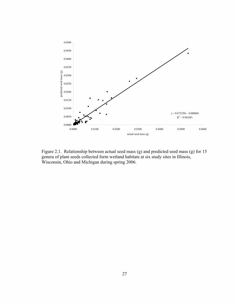
Figure 2.1. Relationship between actual seed mass (g) and predicted seed mass (g) for 15
genera of plant seeds collected form wetland habitats at six study sites in Illinois, Wisconsin, Ohio and Michigan during spring 2006............................. 27
Figure 2.2. Relationship between percent fiber content and true metabolizeable energy (TME) for 22 genera of seeds.. .......................................................................... 29
Figure 3.1 Seed and invertebrate densities with standard errors in wetland habitat types,
pooled across study sites and sampling periods. Samples were obtained in wetland habitats in Upper Mississippi River and Great Lakes Region during February-May 2006. .......................................................................................... 46
Figure 3.2. Seed and invertebrate densities during early (before arrival of migrating waterfowl) and late(after departure of migrating waterfowl) sampling periods, pooled across study sites and habitat types........................................................ 46
Figure 3.3. Seed and invertebrate density at study sites, pooled across sampling periods and habitat types. ............................................................................................... 48
Figure 3.4. Mean % invertebrates of total benthic biomass (kg/ha) in Palustrine emergent (A), Palustrine forested (B) and Lacustrine (C) wetlands sampled in the Upper Mississippi River and Great Lakes Region during February-May 2006 ........... 51
Figure 3.5. Mean % invertebrates of total nektonic biomass (kg/ha) in Palustrine emergent (A), Palustrine forested (B) and Lacustrine (C) wetlands sampled in the Upper Mississippi River and Great Lakes Region during February-May 2006. ................................................................................................................. 53
Figure 3.6. Energetic carrying capacity estimates (DUD/ha) +/- standard errors for ECCu and ECCw at the Scioto River, Lake Erie Marshes and Saginaw Bay Study sites in wetland and cropland habitats during February-May 2006. .......................... 59
Figure 3.7. Energetic carrying capacity estimates (DUD/ha) +/- standard errors for ECCu and ECCw at the Cache River, Illinois River and East Central Wisconsin Study sites in wetland and cropland habitats during February-May 2006. .................. 60
Figure 3.8. Contribution of cropland, lacustrine, palustrine forested, and palustrine emergent habitats to potential duck use days assuming no foraging threshold (none) and three theoretical thresholds at six study sites in the Upper Mississippi River and Great Lakes Region, USA, during February-May
2006…………………………………………………………………………….61

xiii
Figure 3.9. Total potential duck use days that wetlands habitats could support assuming energy, diet, and habitat requirements of dabbling, grazing, diving, and teal foraging guilds at six study sites in the Upper Mississippi River and Great Lakes Region, USA, during February-May 2006 ........................................................ 62
Figure 3.10. Energetic carrying capacity (weighted) +/- standard errors and mean observed waterfowl use/ha on palustrine emergent, palustrine forested, and lacustrine wetlands and croplands at Scioto River (A), Lake Erie (B) and Saginaw Bay (C) study sites during February-May 2006.................................. 63
Figure 3.11. Energetic carrying capacity (weighted) +/- standard errors and mean observed waterfowl use/ha on palustrine emergent, palustrine forested, and lacustrine wetlands and croplands at Cache River (A), Illinois River (B) and East-central Wisconsin (C) study sites during February-May 2006.................. 65
Figure 4.1. Frequency distribution of seeds, tubers, and invertebrates (kg/ha, dry mass)
from a multistage sample of palustrine emergent, palustrine forested, and lacustrine wetland habitats at six study sites in the Upper Mississippi River and Great Lakes Region, USA, during February-May 2006 .................................... 75
Figure 4.2. Total biomass (seeds + invertebrates + tubers) by habitat type combined across all sites using multi-stage sampling (MSS), simple random sampling (SRS), median, and geometric mean estimates.................................................. 76
Figure 5.1. Energetic carrying capacity (kcal/ha) differences between the Upper
Mississippi River Great Lakes Region Joint Venture’s Habitat conservation strategy and my estimates (with 95% confidence intervals). ........................... 84
Figure 5.2. Habitat required to meet the desired species population objectives set forth by the Upper Mississippi River Great Lakes Region Joint Venture’s Habitat conservation strategy. ...................................................................................... 86

CHAPTER 1
INTRODUCTION
The Upper Mississippi River and Great Lakes Region (UMRGLR) is an important
migration corridor for nearly 12 million waterfowl and accounts for nearly 500 million
waterfowl use-days annually (Soulliere et al. 2007). The UMRGLR is located between
two important waterfowl wintering areas (Mid-Atlantic Coast and the Mississippi
Alluvial Valley), and the important breeding areas of the Prairie Pothole and Boreal
Forest regions in the northern U.S. and Canada. A variety of wetland systems occur
throughout the UMRGLR including palustrine, lacustrine, and riverine wetlands
(Cowardin et al. 1979). Glaciated lakes, depressions, and beaver (Castor canadensis)
ponds comprise most of the habitat in the northern UMRGLR, while habitat in the
southern portion is primarily floodplain wetlands, man-made reservoirs and the major
river systems of the Mississippi and Ohio rivers (Soulliere et al. 2007). Coastal marshes
of Lakes Superior, Michigan, Erie and Huron also contain > 15,000 ha of wetland habitat
(Bookhout et al 1989).
Wetland loss in the UMRGLR has been and continues to be substantial. Less
than 15% of historic wetland habitat remains in Ohio, Iowa, Indiana, and Illinois (Dahl
2006). Most wetland loss in rural areas is caused by agricultural conversion (Frayer et al
1983). However urban development and expansion are the leading causes of wetland loss
2
in densely populated areas (Ducks Unlimited 2005). The uncertain consequences of
global climate change and spread of exotic or invasive species also place increasing
pressures on remaining wetlands in the UMRGLR (Johnson et al. 2005).
Historically, waterfowl research focused on the breeding grounds, as populations
were thought to be primarily driven by conditions experienced here. Species distribution,
habitat relationships, and diets of waterfowl were all intensively examined (Trauger and
Stoudt 1978, Bellrose 1979, Swanson et al. 1979). However, habitat conditions and
nutrient resources encountered during the non-breeding period have been linked to
subsequent breeding success and other fitness-related measures, such as survival and
recruitment (Ankney and MacInnes 1978, Hepp 1984, Hohman et al. 1988, Batt et al.
1992, Zimin et al. 2002, Devries et al. 2008). Thus, much research emphasis shifted to
the non-breeding period. Here, most studies were predominately conducted during
autumn and winter because of its importance to over-winter survival and managing
harvest (for review see Weller 1988).
Recent population modeling of mallards (Anas platyrynchos) has demonstrated
that population growth (λ) is most sensitive to nest success, duckling survival, and non-
breeding survival (Hoekman 2002, Coluccy 2008). Devries et al. (2008) examined
individual reproductive investment and nesting success of mallards in the prairie-
parklands of Canada. Their results showed that females with better body condition when
arriving on the breeding grounds had higher nesting propensity and clutch sizes, as well
as earlier nest initiation and hatch dates compared to females in poorer body condition.
Thus, the ability of waterfowl to secure nutrients during spring migration should have a
direct effect on population growth rates (Afton 1984, Anteau and Afton 2004, Newton

3
2006). Indeed, the importance of food availability at spring stop-over sites, when birds
are preparing for the ensuing nesting period, has been demonstrated (LeGrange and
Dinsmore 1988, Jorde et al. 1995, Anteau and Afton 2008). Until recently, autumn and
winter were assumed to be the most limiting portion of the non-breeding season to
sustaining growth of waterfowl populations, however a great deal of attention has shifted
to better understand how habitat factors during spring migration might limit waterfowl
population growth rates.
Despite the potential importance of spring migration, relatively little is known
regarding spring stopover ecology, which continues to be one of the least studied aspects
of avian migration (Lindstrom 1995, Yerkes et al. 2008). In particular, there are few
studies of food availability for waterfowl during spring migration (but see LeGrange and
Dinsmore 1985, DeRoia and Bookhout 1989) although numerous studies have measured
food abundance during autumn migration and winter (Manley et. al. 2004, Boyer et. al.
2005, Stafford et al. 2006a, Brasher et al. 2007, Kross et al. 2008).
Quantity and quality of habitats that waterfowl encounter during spring migration
may differ from autumn migration. Heavy rains and melt-water from winter snowfall
flood crop fields, wetlands, and forested bottomlands during spring. In addition, most
emergent wetlands have considerably different characteristics in spring compared to
autumn as non-persistent emergent and submergent vegetation senesces, falls into the
water column, and decays overwinter. This changes the structure and density of
vegetation in palustrine emergent and aquatic bed wetlands (Galatowitsch and van der
Valk 1996). The decaying plant matter also supports blooms of invertebrates that
become available to spring-migrating waterfowl as they move northward (Euliss and

4
Grodhaus 1987). Waterfowl utilize these flooded habitats as they migrate northward,
accumulating energy and nutrients required for the subsequent breeding season
(LeGrange and Dinsmore 1988, Heitmeyer 2006). Availability of plant foods to spring-
migrating waterfowl likely varies among wetlands with decomposition rates, substrate
firmness, and consumption by non-waterfowl species (Nelms and Twedt 1996, Greer
2006). Although spring flooding may increase habitat availability for spring-migrating
waterfowl relative to autumn, abundance and quality of plant food for waterfowl could be
greatly reduced near the end of winter when waterfowl need nutrients to begin spring
migration. The degree to which invertebrate populations compensate for overwinter loss
of plant food is unknown.
Indeed, food resources have been found to be less abundant in spring compared to
autumn. Greer et al. (2007) demonstrated that spring-flooded impoundments had low
food abundance compared to fall-flooded, likely due to depletion by wintering waterfowl.
Brasher et al. (2007) demonstrated a similar pattern in central and northern Ohio as
wetlands sampled during spring had far less food energy compared to autumn. In
addition, some plant seeds partially decompose, thereby diminishing the energy and
nutrient contents of plant food resources (Nelms and Twedt 1996). Rising water levels
during spring limit foraging opportunities for dabbling and other shallow water foraging
species, though may create foraging opportunities for species that forage in deeper water
(Fredrickson and Drobney 1979, Riley and Bookhout 1993).
Food abundance varies among wetland habitats (Bowyer et al. 2005, Greer et al.
2007, Johnson 2007). Factors such as hydrology, vegetation structure, disturbance,
management regime, soils, and substrate composition all affect food availability. Seed
5
resources are usually most abundant in managed moist soil impoundments where water
levels are manipulated to promote growth of high-yielding moist soil plant seeds and
tubers (Fredrickson and Taylor 1982), although passively-managed wetlands also
produce abundant food (Brasher et al. 2007). Invertebrate abundance fluctuates within
and among seasons (Murkin and Kadlec 1986, Anteau and Afton 2008). Unlike over-
wintering seeds and tubers, invertebrates are continually renewed as populations emerge
and grow. Thus, the standing crop of invertebrates at any single point in time
underestimates the total quantity of food resources available to supply energy and protein
to spring-migrating waterfowl.
Collectively, seeds, tubers, and invertebrates provide the necessary energy and
nutrients for spring-migrating waterfowl. Plant seeds and tubers typically provide more
true metabolizable energy (TME) in the form of carbohydrates (Baldassarre and Bolen
2006), while invertebrates are an essential source of protein (Krapu and Swanson 1975).
While carbohydrates are readily converted into lipids that are mobilized for energy
needed during migration and nesting (Ricklefs 1974), protein is especially important in
late spring and summer when hens lay nutrient-rich eggs (Krapu 1981).
Most waterfowl begin to switch from a diet of primarily plant material that is high
in carbohydrates to an invertebrate diet with high protein near the end of winter, during
spring migration, or after arriving on nesting grounds (Taylor 1978, Heitmeyer 1985,
Lovvorn 1987, Miller 1987, Gammonley and Heitmeyer 1990, but see Gruenhagen and
Fredrickson 1990). The timing of this dietary shift is unknown and likely varies with
species. Hitchcock (Southern Illinois University personal communication) found that
lesser scaup (Athya affinis) consumed higher proportions of invertebrates as they moved
6
north during spring migration. There is conflicting evidence from food habit studies,
whether the transition to a high protein diet occurs during spring migration because
nutritional requirements change, or due to declining abundance of high-carbohydrate
plant foods (Lovvorn 1987). Smith (2007) found that lesser scaup and mallards collected
during spring consumed primarily plant matter, although plant matter was less abundant
where ducks foraged than animal matter. In contrast, Pederson and Pederson (1983)
found that mallards in March and April consumed foods in proportion to their
availability. Although spring-migrating waterfowl utilize both plant and invertebrate
food resources extensively to obtain energy and nutrients, the extent and timing with
which these resources become available to waterfowl in the UMRGLR is unknown.
The Upper Mississippi River and Great Lakes Region (UMRGLR) Joint Venture
has taken a lead role in conservation planning for waterfowl and their habitats in the
region. The UMRGLR Joint Venture boundaries encompass the Great Lakes marshes
and the Ohio, Illinois, upper Mississippi, and lower Missouri river systems (Figure 1.1).
The UMRGLR Joint Venture strives to conserve and enhance critical habitat to meet
breeding waterfowl population goals established by the North American Waterfowl
Management Plan (NAWMP).
The UMRGLR Joint Venture and other non-breeding habitat Joint Ventures have
developed a landscape level bio-energetic approach which seeks to identify the amount of
foraging habitat required to meet waterfowl population goals set by the North American
Waterfowl Management Plan (NAWMP), and to prioritize areas for habitat protection,
restoration, and enhancement. The bioenergetics approach requires understanding of
food energy abundance of habitats and daily energetic requirements of ducks. The
7
UMRGLR Joint Venture has utilized this approach to calculated carrying capacity (i.e.,
duck use days/ha [dud/ha]) estimates that are used to derive habitat objective required to
support breeding population goals of NAWMP. Previous evidence suggests that
waterfowl may be limited by available food energy during spring (Brasher et al. 2007).
Consequently, the UMRGLR Joint Venture recently shifted its focus from autumn
migration to providing adequate habitat for wintering and spring-migrating waterfowl.
The bioenergetics approach assumes that waterfowl can access and consume all
food items within all suitable habitats they encounter during spring migration. More
realistically, species-specific differences in preference and utilization of individual food
items and habitats are well documented (Nudds 1983, DuBowy 1988). Daily energy
requirements of waterfowl also vary among and within species with body mass and
composition (Miller and Eadie 2006). Furthermore, current recommendations for the
UMRGLR Joint Venture waterfowl conservation strategy are derived from small-scale
studies that focused strictly on plant food resources (Korschgen et al 1988, Heitmeyer
1989, Steckel 2003, Boyer et al. 2005, Stafford et al. 2006a). Other NAWMP joint
venture regions have undertaken large-scale assessments of habitat carrying capacity.
Stafford et al. (2006a) and Kross et al. (2008) estimated moist soil seed and rice
abundance across the Mississippi Alluvial Valley. However, to my knowledge no study
has attempted to estimate energetic carrying capacity from plant and invertebrate food
resources over a broad range of wetland and agricultural habitats on a large regional scale
such as the Upper Midwest. More precise measures of food energy abundance and
patterns of temporal and spatial variation in plant and invertebrate food abundance in
different habitat types will strengthen the biological foundation of habitat conservation

Figure 1.1. Locations of study sites within the Upper Mississippi River/Great Lakes Region Joint Venture where energetic carrying capacity was estimated during February-May 2006.
8
9
strategies for the UMRGLR Joint Venture, allowing conservation planners to more
efficiently anticipate waterfowl habitat needs and target priority areas for future
protection, restoration, and enhancement efforts. Undoubtedly, large-scale studies are
needed to direct wetland conservation efforts over broad geographic regions to
complement what has been learned at local scales (Flather and Sauer 1996, Haig 1998).
Therefore the specific research questions I addressed include; 1) what factors are
most important in explaining variation in food density in habitats utilized by spring-
migrating waterfowl? 2) What is the relative contribution of invertebrates to total food
biomass and do invertebrates increase in abundance over time? 3) Do energetic carrying
capacity estimates accounting for guild-specific requirements differ from the more
traditional approach to estimating carrying capacity? 4) Do observed waterfowl
utilization rates exceed energetic carrying capacity estimates, indicating that food energy
may be a limiting factor during spring migration? The following research objectives
were pursued to answer these questions:
1) Identify factors (i.e., study site, habitat type, sampling period) explaining
variation in seed and invertebrate food density (kg/ha).
2) Precisely (CV <15%) estimate food density (kg/ha) from both plant and
invertebrate food sources for spring-migrating waterfowl in four habitat types.
3) Compare changes in relative contributions of plant and invertebrate food
sources to total food biomass over time, sites, and habitats.
4) Compare two models of energetic carrying capacity and explore potential
differences in these methods in relation to importance of conservation planning in the
UMRGLR.

10
5) Compare energetic carrying capacity (dud/ha) with observed waterfowl
utilization rates (bud/ha) of wetlands and croplands habitats.
11
CHAPTER 2
STUDY AREAS AND METHODS
I selected six study sites in four states based on their importance as mid-migration
stopover sites for waterfowl (Figure 1.1). These sites were purposively selected to
provide two latitudinal cross-sections of north-south migration paths within the
UMRGLR. The western study sites included the Cache River region of southern Illinois,
the Illinois River region of central Illinois, and the southeastern glaciated region of east-
central Wisconsin. The eastern study sites from south to north included the Scioto River
in south-central Ohio, the western Lake Erie marshes of northern Ohio, and the eastern
shore of Saginaw Bay in Michigan. Jurisdictionally, all sites were within the Mississippi
Flyway. The majority of waterfowl that use this region are from birds using the
Mississippi River corridor (Bellrose 1968) but there is also a large influx of waterfowl
from the Atlantic coast (T. Yerkes personal communication). Habitat types and amounts
varied by study site (Table1.1). According to National Wetland Inventory (1990) data
(NWI), the Illinois River site had the most wetland area (> 14,000 ha) while the Scioto
River site had the least (< 1,000 ha). Palustrine forested wetlands were the most
abundant wetland type at the Cache and Illinois River sites; palustrine emergent wetlands
were most common in the east-central Wisconsin, Lake Erie marshes, and Saginaw Bay
sites, while lacustrine habitat was most prevalent at the Scioto River site. Agriculture

12
Study Site Habitat Type Source Area (ha)Cache River palustrine-forested NWI 4,608 palustrine-emergent NWI 790 lacustrine NWI 141 cropland SMI 6,215 Illinois River palustrine-forested NWI 7,717 palustrine-emergent NWI 2,143 lacustrine NWI 4,450 cropland SMI 4,959 Wisconsin palustrine-forested WWI 1,608 palustrine-emergent WWI 6,004 lacustrine WWI 180 cropland SMI 20,109 Scioto River palustrine-forested NWI 259 palustrine-emergent NWI 274 lacustrine NWI 413 cropland SMI 2,075 Lake Erie Marshes palustrine-forested NWI 2,010 palustrine-emergent NWI 2,130 lacustrine NWI 1,854 cropland SMI 7,369 Saginaw Bay palustrine-forested NWI 1,080 palustrine-emergent NWI 13,150 lacustrine NWI 6 cropland SMI 3,048
Table 1.1. Waterfowl habitat areas (ha) at six study sites in the Upper Mississippi River and Great Lakes Region where energetic carrying capacity was estimated during February-May 2006. Source: National Wetlands Inventory (NWI), Wisconsin Wetlands Inventory (WWI) and Ducks Unlimited, Inc. Soil Moisture Index (SMI).

13
was the predominant land use at all six sites. The UMRGLR experiences a wide range of
annual climatic conditions that influence the length of the growing season, the number of
ice-free days, and surface hydrology. As a result waterfowl use of this area is closely tied
to seasonal and annual variation in weather conditions (Reid et al 1989, Stafford et al.
2007). The UMRGLR Joint venture implementation plan (1998) has designated each
site as a focus area in recognition of their regional significance as waterfowl habitat.
Each study area encompassed approximately 520 km2. Study site boundaries were
oriented to capture the major hydrologic features (i.e., major rivers, lake shorelines and/or
wetland complexes) and representative habitat types at each site.
Cache River The Cache River site, centered near Cairo, IL, included a 44 km reach of the
lower Cache River and Cypress Creek. The Cache River watershed encompasses 927
km2 with elevation 85 – 102m above sea level. Mean annual temperature is 13.7 C, with
average winter temperatures ranging from 3.2 – 8.3 C, and spring temperatures ranging
from 8.5 – 18.8 C (Illinois State Water Survey 2008). Mean annual rainfall is 122.7 cm;
greatest precipitation occurs in late winter and spring (Illinois State Water Survey 2008).
The lower Cache River is highly modified and its hydrology differs from the
upper section. Channel modifications have introduced major changes to the Cache
River’s hydrology over the past 100 years. The Post Creek Cutoff constructed around
1915 diverted water from the Cache River which now flows directly into the Ohio River.
The Cache River floodplain is bordered by upland deciduous forests consisting of oaks
(Quercus spp.) and hickories (Carya spp.) with interspersed rocky bluffs. Most (68%) of

14
the lower cache river floodplain has been cleared for agriculture (Hutchison 1987,
Demissie et al. 1990). Forested wetlands characterize the Cache River floodplain, with
70% identified as bottomland hardwood forest and 16% as bald cypress (Taxodium
distichum) swamp totaling over 5,497 ha collectively (Havera 1999). In fact, the
watershed encompasses most of the remaining bald cypress swamps in southern Illinois
(Dorge et al. 1984).
The Cache river floodplain is important for waterfowl and other birds as over 250
species occur within the region. The RAMSAR Convention designated the Cache River
a wetland of international importance. The wetlands reserve program (WRP) has
increased managed wetland areas in recent years. The Frank C. Bellrose federal
waterfowl reserve, within the Cypress Creek National Wildlife Refuge, is managed to
provide migratory waterfowl and shorebirds with moist soil habitats where water level
are manipulated and periodic mechanical disturbance is used to promote growth of
desirable wetland food plants.
Illinois River
The Illinois River study site is centered near Chandlersville, IL along a 45 km
reach of the Illinois River and includes part of Chautauqua and Emiquon National
Wildlife Refuges, and Sanganois and Anderson Lake public wildlife areas. Mean annual
temperature is 10.8 C with average winter temperatures ranging from -1.9 – 4.8 C , and
spring temperatures ranging from 4.4 –16.9 C (Illinois State Water Survey 2008).
The Illinois River is historically known as one of the most important areas for
migrating waterfowl in all of North America (UMRGLR Joint Venture Management

15
Board 1998). The Illinois River has been greatly altered since it was impounded and
dredged for navigation in the early 1900s. Sediments from farmed uplands in the
watershed are now deposited in floodplain lakes when river levees are overtopped during
flood events. Prior to human alteration, natural flows of clear water allowed growth of
emergent and submergent waterfowl food plants in backwater lakes and side-channels of
the Illinois River floodplain. Runoff from surrounding uplands, and sediment transported
into side-channels and bottomland lakes during Illinois River flood events has created
turbid conditions, soft substrates, and sedimented backwater lakes. In addition, exotic
fish (e.g. Cyprinus spp.) stir up bottom sediments, uproot vegetation, and re-suspend
contaminants, leading to secondary loss of wetland vegetation. Floodplain forests have
also changed from hard to soft-mast producing species (Havera 1999). The natural flood
pulse pattern essential to that system is presently impaired (Sparks et al. 1998; Koel &
Sparks 2002). The river now has unnaturally high water levels in the summer, with
several minor floods in midsummer that often drown moist-soil plants.
Despite these large scale changes in environmental quality, the Illinois River
floodplain still serves as an important migration staging area for waterfowl each year.
Chautauqua NWR has been designated a Western Hemisphere Shorebird Network Site
and a Globally Significant Bird Area (Havera 1999). The Chautauqua NWR supports
roughly 45% of waterfowl use of the Illinois segment of the Mississippi Flyway and
nearly 70% of the waterfowl that use the Illinois River Corridor (USFWS 2004). Over
1.5 million mallards have been recorded using the area during one census period (Havera
1999).

16
East-central Wisconsin
This site was located near Waupun, WI in the Upper Rock River watershed in
southeastern Wisconsin, including portions of the Horicon National Wildlife Refuge and
extending into Dodge and Fond du Lac counties. Mean annual temperature is 7.6 C, with
average winter temperature ranging from -1.9 – -6.3 C and spring temperatures ranging
from 0.2 –14.3 C (Midwest Regional Climate Center 2008). Mean annual rainfall is 83.9
cm; greatest precipitation occurs in late summer and early fall (Midwest Regional
Climate Center 2008).
Surrounding land use consists largely of highly productive agriculture supported
by rich peaty soils and glacial outwash. Most of the agricultural land is used for dairy
farming. Wetland habitat in this area of Wisconsin is predominately cattail (Typha spp.)
marsh, although some wetlands are managed to promote hemi-marsh habitat. The most
recent glaciations created numerous pothole wetlands which are attractive sources of
breeding habitat for many waterfowl. In fact, this site has the most significant numbers
of nesting blue winged teal, mallards and some diving ducks, compared to my other study
sites (Van Horn and Gatti 2006). Dodge and Fond du Lac counties, including the
Horicon area, are only 7 and 11% forested, respectively (Craven and Hunt 1984).
The Horicon Marsh system is considered the largest cattail (Typha spp.) marsh in
the United States. The marsh consists of a shallow basin drained by the Rock River. The
northern 8,367 ha is managed by the U.S. Fish and Wildlife Service as Horicon NWR and
the remainder is managed by the Wisconsin Department of Natural Resources. There are
216 species of birds that commonly use Horicon Marsh. Another 32 species occasionally
occur there (USFWS, 1994). Recognizing the diversity of flora and fauna and the large
17
populations of waterfowl that Horicon Marsh supports, the RAMSAR convention
designated Horicon Marsh as an Wetland of International Importance in 1990 (Davis
1994). However, severe problems continue to threaten the habitat resources of Horicon
marsh. The most severe problem is siltation due to soil erosion from surrounding
watersheds. Other major problems include rough fish infestation (mainly Cyprinus
carpio), purple loosestrife (Lythrum salicaria) infestation, high inflow of nutrients
(primarily phosphorous) into the marsh from surrounding farms, pastures and barnyards,
and overall loss of native vegetation communities.
East-central Wisconsin has been identified as the region of Wisconsin that
contains the majority of migratory habitat for waterfowl (UMRGLR Joint Venture 1998).
The importance of this region for migration, staging and nesting Canada geese (Branta
canadensis) has been well documented (Craven and Hunt 1984, Heinrich and Craven
1992), and is also important for many duck species (Stollberg 1950, VanHorn et al. 2006,
Wisconsin Department of Natural Resources 2008).
Scioto River
The Scioto River study site was centered on a 45 km segment of the Scioto River
approximately 15 km south of Columbus, OH. Mean annual temperature is 10.5 C with
average winter temperatures ranging from -3.06 – 5.67 C, and spring temperatures
ranging from -1.11 – 15.5 C (Midwest Regional Climate Center 2008). Mean annual
snowfall is 36.1 cm, with highest snowfalls in January, and the mean annual rainfall is
99.1 cm (Midwest Regional Climate Center 2008).
18
The Scioto River area has numerous flat plains, many of which have been cleared
and farmed, and numerous small streams that remain open in winter and are tributaries to
the larger Scioto River. The lower Scioto River valley is very large compared to the
width of the river itself where melt-waters from retreating Ice Age glaciers carved the
valley exceptionally wide. Besides being Ohio's longest river, the Scioto River
Watershed is home to more species of fish and mussels than any other Ohio watershed.
Principal wetland areas within the site include Stage’s Pond Nature Preserve, which
encompasses two glacially formed kettle lakes and surrounding wetland communities,
and Calamus Swamp, a primarily cattail marsh. Forested wetlands are primarily
restricted to the banks of the Scioto River and Big Darby Creek. Despite the lack of
wetland area, there are hundreds of hectares of private land enrolled in the Conservation
Reserve Enhancement Program (CREP). So far, farmers have enrolled more than 22,000
ha in 15-year conservation agreements throughout the 1.6 million-hectare Scioto River
Watershed (The Nature Conservancy 2008). Flooded CREP areas provided access to
abundant food resources and increased the amount of usable habitat for waterfowl. Since
many of these CREP fields are within the Scioto River floodplain , they often become
inundated with floodwater during late winter and spring.
The Scioto River study site had the smallest total wetland area (946 ha) among the
six study sites, so this area’s importance to waterfowl is not well understood. Most of
this is the Scioto River itself. However the Scioto river valley likely serves as important
American black duck (Anas rubripes) and mallard wintering and migration habitat
(UMRGLR Joint Venture 1998).
19
Lake Erie Marshes
The Lake Erie site was located about 2 km South of Port Clinton, Ohio, centered
around Sandusky Bay, Ohio. Mean annual temperature is 10.6 C with average winter
temperatures ranging from 0.4 – 2.9 C, and spring temperatures ranging from 3.6 – 15.8
C. Mean annual snowfall is 25.9 cm, with highest snowfalls in January, and the mean
annual rainfall is 95.6 cm.
The western Lake Erie marshes historically consisted of freshwater tidal marshes
bordering the Sandusky and Muddy Creek Bays. High water levels over the past several
decades have eradicated these naturally occurring marshes and current wetlands are
mostly impounded marshes actively managed by the Ohio Department of Natural
Resources Division of Wildlife, U.S. Fish and Wildlife Service or private waterfowl
hunting clubs. A landscape matrix of tiled agricultural fields surrounds Sandusky Bay,
leaving very little ephemeral flooded agricultural habitat; although many hunt clubs
actively flood croplands in the fall (Olson 2003, Baranowski 2007). The Winous Point
Marsh Conservancy (WPMC), located near the center of the Lake Erie site is the first
private duck hunting club in North America. WPMC consists of 570 ha of wetland
habitats and harbors thousands of waterfowl and shorebirds during fall and spring
migration (Farney 1975, Olson 2003, Steckel 2003, Baranowski 2007). The Lake Erie
marshes have always been important migration areas for waterfowl (Bookhout 1989).
Aerial surveys conducted by the Ohio Division of Wildlife confirm that hundreds of
thousands of waterfowl heavily use habitats in this region during both autumn and spring
migrations.
20
Saginaw Bay
The Saginaw Bay study site was centered near Sebewaing, MI on the eastern
shore of Saginaw Bay between Fish Point State Game Area and Sand Point. Mean
annual temperature is 7.06 C, with average winter temperatures ranging from to -6.11 –
3.11 C, and spring temperatures ranging from -5.33 – 11.5 C. Mean annual snowfall is
85.6 cm and mean annual rainfall is 66 cm with the greatest precipitation occurring in late
summer (Midwestern Regional Climate Center 2008).
The study site emcompassed shallow waters within 5 km of the Lake Huron
shoreline, including Wildfowl Bay, and adjacent uplands and inland marshes < 5 km
from the shoreline. Several barrier islands with wetland and upland habitats were
included in the study site, including Middle Grounds, Heisterman, Maisou, Defoe,
Pitcher’s Reef, and Lone Tree Islands. These islands formed a boundary between the
shallower waters east of the islands and deeper water to the west. Water levels fluctuate
seasonally and daily, typical of freshwater coastal marshes (Bishop 1990). The highest
water levels occur when prevailing winds are from the north to northeast, while low
water levels occur during a south to southwest wind. Bottom sediments throughout the
bay range in size from large pebbles to clay, while medium to fine grained quartz sand is
also common (Wood 1964). Nalepa et al. (1995) estimated that 70% of the bottom
consists of sand, cobble, and gravel and 30% consists of silt/mud within the shallow
waters of inner bay.
The adjacent upland is largely rural and land use is primarily agriculture. Poorly
drained, nutrient rich loamy soils underlie most of the area. Nearly all of the agricultural
fields have been tiled to promote rapid run-off of surface water, discharging sediments
21
into the bay. Major drainage systems include the Sebewaing River, Pigeon River, several
wide sand channels formed from glacial melt-water streams, and many man-made
channels including the Shebeon drain (Smith 1901).
Wetland habitats are primarily associated with the shallow waters of Saginaw Bay
and at Fish Point WA. The National Wetlands Inventory (NWI) identified >13,150 ha of
coastal wetland habitat as seasonally emergent wetland. These habitats typically lack
submergent vegetation and are dominated by bulrush (Scirpus spp.) in spring. Much of
the wetland habitat identified by the NWI has been destroyed due to wave action and
discharge of sediments into Saginaw Bay from adjacent croplands. In addition, common
reed (Phragmites australis) a non-native species has colonized and displaced much of the
native vegetation in these habitats. Cropland dominates the upland habitats; three main
crop types grown in the area including corn (Zea mays), soybean (Glycine max), and
sugar beet (Beta vulgaris).
22
METHODS
Food Sample Collection
Sampling Design and Allocation
I used a Geographical Information System (GIS) to overlay 2,292 16-ha square
grid cells over combined wetlands inventory and soil moisture index (SMI) coverages of
each study site. I used the Wisconsin Wetlands Inventory (WWI; Johnnston 1984) to
identify wetlands at the Wisconsin study site and The National Wetlands Inventory
(NWI; National Wetlands Inventory 1990) for all other sites. The source date of imagery
used for both the NWI and WWI varied from 1978 –1984. Grid cells with > 0.8 ha of
wetland habitat were classified into one of three sampling strata based on wetland habitat
and wet soil composition. I chose this size threshold to increase the chance of
encountering wetlands within a cell in the field since NWI and WWI can potentially
misclassify smaller wetlands (Tiner 1997). I similarly classified the remaining cells as
cropland cells when they contained >8 ha of cropland identified as “prone” to flooding by
the SMI coverage (Ducks Unlimited 2005a). Wetland cells took priority over cropland
cells because cropland was the dominant land-use at all sites thus at some sites there
would not have been enough wetland cells to take an adequate sample from. Cells that
contained < 0.8 ha of NWI data and < 8 ha of SMI were not included in my sampling
design. At the Illinois River study site, adequate samples could not be obtained from

23
selected cells so I drew samples from habitats outside my selected cells. These samples
were selected by convenience sampling but were selected in proportion to the amounts of
habitat in the area.
I further stratified wetland cells based on the predominant wetland type
(Cowardin et al. 1979) within the cell. Wetland cells were classified as palustrine
emergent (PEM), palustrine forested (PF), or lacustrine (LC). I used the Animal
Movements extension in ArcView 3.3 (Hooge and Eichenlaub 1997) to randomly select
wetland and cropland cells from each study site. Wetland cell types (i.e., PF, PEM, LC)
were selected in proportion to their availability at each study site. Therefore, my
sampling frame represented 16 ha cells, where there was at least 0.8 ha of wetland or
cropland habitats potentially usable by waterfowl.
I ground-truthed cells to determine the types of habitats actually present within
each randomly selected cell using a Dell PDA 750 with ArcPad (ESRI 2001). I classified
and confirmed wetlands within cells as palustrine forested (PF), palustrine emergent
(PEM) or lacustrine (LC) based on their hydrological characteristics and dominant
vegetation present at the time of each visit following the criteria of Cowardin et al.
(1979). I classified cropland (AG) habitats according to the crop type present. I used
maps with aerial photographs of the cell to delineate the boundaries of all habitat types
during each visit to a cell. Interpreting these maps and aerial photographs, I also
estimated the percentage of the wetland that was >30 cm deep. At each site a number
quota of food samples was identified based on processing capacity in the laboratory. I
sampled only as many cells as necessary to fill the quota. All or nearly all cells were
surveyed for waterfowl use, whereas a subset of cells was used to obtain food samples.
24
Wetland Food Biomass
Sampling dates varied by study site, depending on timing and duration of passage
of waterfowl through each site during spring 2006. A pre-migration sample was always
taken immediately following ice-thaw, before migrating waterfowl arrived. A post-
migration food sample occurred after most waterfowl departed from each study site
(Appendix 1). I determined migration chronology from observed waterfowl use on my
study cells. I randomly selected wetlands in proportion to their occurrence within a
particular study site to estimate biomass (kg/ha) of both plant and invertebrate food items.
I obtained two samples from shallow (< 30 cm) and deep (>30 cm) zones of each wetland
except where the deep zone was absent. Thus, I obtained four total samples per wetland
per sampling round for most wetlands. I sampled nektonic biomass by sweeping a d-
frame net (33 cm diameter, 500 μm mesh) in the water column within a 100 cm x 50 cm
x 75 cm, 500 μm mesh side panel drop box. I then sampled benthic biomass by inserting
a core sampler (7 cm diameter) 10 cm into the substrate at a random location within the
drop box. I washed samples in the field using a 500 μm sieve bucket and placed them
into a 3.8 l labeled polyethylene bag containing 10% formalin solution. I categorized
each sampling location into one of four distinct vegetation cover classes (mostly
vegetated, interspersed vegetation, vegetated edges and mostly open water (Stewart and
Kantrud 1971). I recorded the UTM coordinates of the sample location using a Global
Positioning System (GPS).

25
Cropland Plant Food Biomass
I used a technique modified from Frederick et al. (1984) to sample plant food
biomass in cornfields. I randomly placed a 14-m nylon rope perpendicular to planting
rows, and then selected one side of the rope to sample by coin flip. I collected all whole
and partial corn ears that retained grains within 1 m of the rope over a distance of 14 m. I
defined a partial corn ear as one that had at least 1 corn kernel adhering to it. I also
collected individual corn kernels by inserting a core sampler (7 cm diameter) 3 cm into
the substrate placed at five systematic locations along the 14 m rope. I sampled soybean
fields by randomly placing the drop box (100 cm x 50 cm) and collecting (by hand when
not flooded or the d-net when flooded) all soybean seeds that were present within the
box. I placed samples in labeled 3.8 l polyethylene bags. Cropland samples were taken
back to a lab, where they were allowed to air dry before being placed in a convection
oven for 48 hours at 60 C to constant mass.
Laboratory Methods
Wetland food samples collected in the field were sent to Southern Illinois
University at Carbondale (SIUC) where they were hand-picked to separate all non-food
material from waterfowl plant and invertebrate food items. Invertebrates were identified
to family or lower taxonomic level when possible by Richard Schultheis, a PhD candidate
at SIUC. Seeds were shipped back to the lab at Ohio State University where seeds and
tubers were identified to genus (Martin and Barkley 1961, Delorit 1970, Montgomery

26
1977, Davis 1993), sorted, and dried to constant mass at 60 C for 48 hours in a
convection oven before weighing to the nearest 0.0001g. I defined duck food as plant
and invertebrate food items known to be consumed by at least one species of waterfowl
in the UMRGLR (Martin and Uhler 1951, Farney 1975, Havera 1999, Smith 2007). I
counted but did not weigh seeds from the following genera Amaranthus spp., Bidens
spp., Cephalanthus spp., Chenopodium spp, Cyperus spp., Echinocloa spp., Eleocharis
spp., Leersia spp., Najas., Panicum spp., Polygonum spp., Potamogeton spp., Rumex
spp., Sagittaria spp. and Scirpus spp when samples contained < 25 seeds of these genera
to reduce processing time spent on small samples. I used the product of the number of
seeds from each genus and mean seed mass from a representative sample of each genus
to estimate mass to the nearest 0.0001g when samples contained <25 seeds of these
genera. Using average seed mass to predict total sample mass was determined by Arzel
et al. (2007). I always dried and weighed all other seed genera identified as waterfowl
food, and when there were > 25 seeds from the genera listed above. Actual and predicted
seed mass was tightly correlated (Figure 2.1) and there was no difference between actual
and predicted seed mass (paired t (1.88) = -1.01, P = 0.314). I represented biomass
estimates as kg/ha.
y = 0.872359x - 0.000004R2 = 0.901091
0.0000
0.0050
0.0100
0.0150
0.0200
0.0250
0.0300
0.0350
0.0400
0.0450
0.0500
0.0000 0.0100 0.0200 0.0300 0.0400 0.0500 0.0600
actual seed mass (g)
pred
icte
d se
ed m
ass (
g)
Figure 2.1. Relationship between actual seed mass (g) and predicted seed mass (g) for 15 genera of plant seeds collected form wetland habitats at six study sites in Illinois, Wisconsin, Ohio and Michigan during spring 2006.
27

Energetic Carrying Capacity
I converted food biomass estimates to energetic carrying capacity (ECC) by using
published values of true metabolizable energy (TME) for seeds, tubers, and invertebrates
(Appendix 2) as described by Reinecke et al. (1989). I substituted TME values for some
taxa when published estimates were not available with those from the closest taxonomic
group. When crude fiber estimates were available, I regressed % fiber content (Havera
1999) on published TME values (Appendix 3) to estimate TME for taxa without
published estimates (Figure 2.2) after Petrie et al. (1998).
I used two methods to calculate ECC, as one of my objectives was to illuminate
differences in duck species-weighted vs. un-weighted ECC estimates. The un-weighted
ECC estimate, hereafter ECCu, assumes each duck use-day represents a constant daily
energy requirement (DER) of 292 kcal/day (i.e., typical female mallard), and that all
potential food items can be consumed (i.e., no food preferences), from any available
habitat. The formula used to calculate ECCu per habitat type was;
ECCu = ∑ (massi × 1000 × TMEi) )/ 292 kcal/day) =
n
i 1
where ECCu= carrying capacity of (dud/ha), n = total number of food items, massi =
biomass of particular food item (kg/ha), TMEi = true metabolizable energy (kcal/g) of
food item. I derived the weighted estimate of ECC (hereafter ECCw) to account for duck
species-specific DER, food habits, and habitat utilization rates of four separate foraging
guilds. The guilds included dabblers (mallard, American black duck, northern pintail
[Anas acuta], wood duck [Aix sponsa]), divers (lesser scaup, canvasback [Aythya
vallisineria], redhead [Aythya americana], ring-necked duck [Aythya collaris], and ruddy
28

y = -0.0553x + 3.3361R2 = 0.3297
0.00
0.50
1.00
1.50
2.00
2.50
3.00
3.50
4.00
0.0 5.0 10.0 15.0 20.0 25.0 30.0 35.0 40.0 45.0 50.0
& Fiber
TME
Figure 2.2. Relationship between percent fiber content and true metabolizeable energy (TME) for 22 genera of seeds. Percent fiber content values are from (Havera 1999) and TME (kcal/g) values are from various published sources.
29

30
duck [Oxyura jamaicensis]), grazers (American wigeon [Anas americana] and gadwall
[Anas strepera] ), and teal (blue-winged teal [Anas discors], green winged teal [Anas
crecca], and northern shoveler [Anas clypeata]). I estimated a weighted guild-specific
DER by averaging DER of all species in a guild following Miller and Eadie (2006;
Appendix 4) and multiplying by the proportion of each guild observed in a habitat at a
site (Appendix 5). I obtained species-specific food habit data from a concurrent diet
study that focused on mallard, gadwall, blue-winged teal, ring-necked duck, and lesser
scaup (Jay Hitchcock Southern Illinois University–Carbondale; Appendix 6). I assumed
all species of dabblers consumed the same foods as mallards, and similarly substituted
ring-necked duck and lesser scaup diets for all divers, gadwall for grazers and blue-
winged teal for the teal guild. I also assumed diving ducks foraged only in palustrine
emergent and lacustrine wetlands and all food >30 cm depth found in the benthic samples
was available only to divers (Appendix 7). Therefore, the weighted ECCw estimate
should be more representative of energetic carrying capacity because it accounts for
guild-specific food habits, habitat use, and daily energy requirements.
I also computed a guild-specific ECC estimate (hereafter ECCguild) which uses the
same parameters as ECCw but I did not weight the DER by the proportion of guilds using
a habitat at a site. Instead I used a foraging guilds mean DER and assumed all the
biomass in a wetland regardless of the presence of other guilds could only be consumed
by one guild. Thus, this estimate represents the carrying capacity for each specific guild.
Therefore, ECCw and ECCguild were estimated with a deterministic equation based
on estimated guild specific energetic carrying capacities. The model included inputs: (1)
biomass (kg/ha); (2) TME values; (3) daily energy requirements; and (4) proportion of

each guild observed using a particular habitat at each site. The model formula for ECCw
per habitat type was:
31
ECCw = ∑
=
n
i 1
(massi × 1000 × TMEi )
( )∑=
4
1g( DERg × pHg )
where ECCw = carrying capacity (dud/ha), n = total number of food items, massi =
biomass of particular food item (kg/ha) , TMEi = true metabolizable energy of food item i
(kcal/g), DERg = daily energy requirement of a particular guild (kcal/day), and pHg =
proportion guild observed using a particular habitat. The model formula for ECCguild per
habitat type was:
ECCguild = ∑
=
n
i 1
(massi × 1000 × TMEi ) ( )DERg
where ECCguild = carrying capacity (dud/ha), n = total number of food items, massi =
biomass of particular food item (kg/ha), TMEi = true metabolizable energy of food item i
(kcal/g), DERg = daily energy requirement of a particular guild (kcal/day).
Waterfowl have been shown to abandon food patches when food biomass drops
below a certain threshold where it is no longer energetically profitable to search for food
(Reinecke et al. 1989). Several foraging thresholds have been proposed. Reinecke et al.
(1989) suggested that waterfowl were unable to forage profitably on waste rice densities
<50 kg/ha. Naylor (2002) examined post-winter food densities in wetlands, and
concluded that 130 kg/ha was the average foraging threshold, although variability was
high among years. Finally, Hagy (Mississippi State University, personal communication)
found that food levels were greater than 280 kg/ha after waterfowl abandoned moist-soil
wetland sites in Mississippi in late winter. I converted these biomass thresholds to
32
energetic thresholds following Brasher et al. (2007), with corresponding thresholds of
324, 865, and 1,996 dud/ha, respectively.
Waterfowl Use-Days
I censused all waterfowl present in wetland and cropland habitats within the
boundaries of 16 ha study cells at each study site. A minimum of 38 cells were surveyed
per study site and were visited 1-8 times between the first and last food sampling periods.
I did not record ducks that were outside of any study cell even if they occurred on the
same wetland that was partially included in a cell. I used maps with aerial photographs to
determine the boundaries of each cell in the field. I first counted all species via visual
observation using a spotting scope and binoculars and subsequently walked through
dense vegetation to flush ducks that were not visible. Care was taken to avoid double-
counting ducks that flushed from, and landed on, different parts of the survey plots. I
derived estimates of total ducks use-days by averaging the number of ducks (by species)
per survey on each wetland or crop unit present within each wetland or crop unit within
each cell, separately by study site. The mean number of ducks observed/day was
multiplied by the number of days between first and last dates that food samples were
collected at each study site to convert mean counts (a mean of one duck observed on each
wetland within a cell represented one duck use-day) to duck use-days (DUD) over the
entire survey period (35 – 53 days across sites; Appendix 1). Individual estimates of
DUD by all unique combinations of site, cell, and wetland were divided by the estimated
area of each wetland (within sites and cells) to convert DUD estimates to the same units
(DUD/ha) as food energy carrying capacity estimates. These estimates were then
33
averaged within wetland system or crop categories at each site to obtain waterfowl
utilization rates (DUD/ha) for the same habitat systems used to summarize ECC (AG,
PEM, PF, and LC).
Statistical Analyses
Biomass Density Estimates
I used multi-stage sampling (MSS) to estimate abundance of food energy in
wetland and cropland habitats at each site. Multi-stage sampling provides an un-biased
estimate that is particularly appropriate for large-scale natural resource surveys,
especially those with hierarchical nested designs similar to mine (Conroy and Smith
1994, Stafford et al. 2006b.) My sampling design treated cells as primary sampling units,
wetlands and croplands as secondary units, and plots within wetlands and croplands as
tertiary units. I used PROC SURVEYMEANS in SAS version 8.02 to estimate food
density in wetland and cropland habitats. I performed separate analyses for each study
site. I estimated mean food density per wetland system for all sites with sampling
weights derived for each individual study site. I also estimated biomass density pooled
across sites by using site specific sampling weights. I calculated the probability of
selecting a cell by dividing the number of sampled cells by the total number of cells
available at a site. I calculated the probability of selecting a wetland or cropland unit by
dividing the number of sampled wetlands by the number of wetlands or croplands present
within a cell. I calculated the probability of taking a benthic sample by dividing the area
of the core sampler (38.23cm2) by the number of possible cores given the area of wetland
or cropland. I calculated the probability of obtaining a nektonic sample by dividing the
34
area of the drop box (0.5m2) by the number possible given the area of the wetland or
cropland. The inverse of the product of the 3 selection probabilities (i.e., cell,
wetland/cropland, and benthic/nektonic) was the sample weight used in analyses.
SURVEYMEANS uses Taylor series linearization to estimate variances of means (SAS
Institute 1999:3200). In the case of the Illinois River where I took samples outside of my
study cells, I used the mean weight from samples where I did sample within cells at that
site.
Individual datum points in a MSS can have a strong influence on the overall mean
(Gershunskaya and Huff 2004). I examined marginal plots to examine the influence of
individual datum points on the overall means. Marginal plots display box plots of sample
values (i.e., kg/ha) versus sample weights. For each analysis, I adjusted the weight of a
datum point by assigning it the mean weight of the remaining datum points if a marginal
plot identified a datum point as an outlier (i.e., it had both a large sample value and high
weight; California Health Interview Survey 2002).
I calculated percent occurrence of plant food items within wetlands by
determining the frequency of occurrence for seed or tuber taxa within benthic or nektonic
samples, divided by the total number of benthic and nektonic samples. I used PROC
SURVEYMEANS to calculate seed and tuber density estimates in wetlands habitats
summed across all sites. I summed estimates and variances of benthic and nektonic
samples (Stafford 2006a), to provide a single density estimate per habitat type.

35
Variation in plant and invertebrate food abundance
I used the GLM package (Dobson 1990) in R version 2.4.0 (R Development Core
Team 2006) to model the relationships of food abundance as a function of site, sampling
period, habitat type, wetland depth zone, and cover class. I only explored relationships in
benthic samples since density of food items from benthic samples was vastly greater than
nektonic samples and represented the majority of total food biomass (>98%). I
performed two analyses; one each with plant food abundance (kg/ha) and invertebrate
food abundance (kg/ha) as response variables. I designated site, sampling period, habitat
type, wetland depth zone and cover class as fixed explanatory variables. After assessing
the normality of the data and inspecting the residuals vs. the fitted values I log-
transformed my response variable then applied a generalized linear model using a
Gaussian distribution with the identity link.
I used Akaike’s Information Criterion (AIC) to identify candidate models that
best fit the data (Burnham & Anderson 1998). The AIC identifies the most parsimonious
model from a set of candidate models; that is, the model supported most strongly by the
data, given the bias corrected, maximized log-likelihood of the fitted model, and a
penalty for the number of parameters used. This method of model selection counters the
problem of over-fitting and the subsequent loss of precision of parameter estimates. The
AIC values of parameter estimates were adjusted for over-dispersion by calculating a
variance inflation factor. The AIC value adjusted for over-dispersion is termed the
corrected quasi-likelihood AIC (denoted as QAIC). Therefore, I constructed candidate
models based on a priori expectations regarding which variables, combinations of
variables, and interactions might be biologically meaningful. I considered the best model
36
to be the one with the lowest QAIC. I used the results from the QAIC to inform
decisions on which factors were most important in explaining variation of my response
variables and summarized the results accordingly.
Invertebrate contribution
I divided the biomass of invertebrates (kg/ha) by the total biomass (kg/ha) for
individual samples to calculate percent contribution of invertebrates to total food biomass
for each nektonic and benthic sample. I used analysis of variance (ANOVA) in R version
2.4.0 to test for differences in percent invertebrate contribution by study site, wetland
system, and sampling period. I ran separate tests for nektonic and benthic samples. I
used a logistic transformation (log(1/1-x)) to normalize percent invertebrate contribution
and meet distributional assumptions of the test. Logistic transformations are applied to
analyze responses such as mine that are restricted to a finite interval (i.e., 0 – 100%;
Lesaffre et al. 2006).
Energetic Carrying Capacity
I used ANOVA in R version 2.4.0 to test if ECCu and ECCw varied by study site,
habitat type and sampling period. I log transformed (base 10) food energy abundance
estimates to normalize distributions and account for homogeneity of variance prior to
statistical analysis (Quinn and Keough 2002). I used a paired t-test in R version 2.4.0 to
test differences between ECCu and ECCw in each of the 21 habitat by site specific
comparisons.
I used PROC SURVEYMEANS in SAS version 8.02 to estimate ECCu and ECCw
in wetland and cropland habitats. I computed separate estimates at each study site for

37
each habitat type. I examined marginal plots to examine individual datum points and
their influence on the overall means and adjusted weights if a datum point simultaneously
had both a sample value and weight as an outlier (California Health Interview Survey
2002). I multiplied ECCw and ECCguild by the amount of habitat at a particular site
(Table 1.1) to compute species-specific use days a site could potentially support.
38
CHAPTER 3
RESULTS
Percent Occurrence of plant food items
I summarized % occurrence and biomass (kg/ha) density for 37 genera of seeds.
Seeds from the family Cyperaceae (i.e., sedges and rushes) and Poacae (i.e., grasses)
contributed nearly 60% to total seed biomass in PEM wetlands (Table 3.1) Polygonum
spp., Cornus spp. Quercus spp., and Cephalanthus occidentalis, contributed 71% of total
plant biomass in PF wetlands (Table 3.1). Ipomoea spp., Cyperacea, and tubers from
Sagitaria spp. and Cyperus Spp. contributed nearly 50% of total plant biomass in LC
wetlands (Table 3.1). Polygonum spp. was the most frequently occurring seed taxon in
all three wetland habitats I sampled. Collectively they accounted for 7.4%, 24.6%, and
6.3% of total plant biomass in PEM, PF, and LC wetlands respectively.
Nektonic food biomass
I sampled 110 PEM wetlands, 84 PF wetlands and 76 LC wetlands across all sites
(Table 3.2). Total food density was greatest in PF wetlands (4.84 kg/ha), followed by
PEM wetlands (2.49 kg/ha), and LC wetlands (0.58 kg/ha; Table 3.2) across all sites.
Within study sites, CVs were mostly greater than my desired level of precision (CV ≤
15%); however, for the total food density combined sites the CVs for PF samples were
the only ones to exceed CV = 15% (Table 3.2). Seed and invertebrate densities were
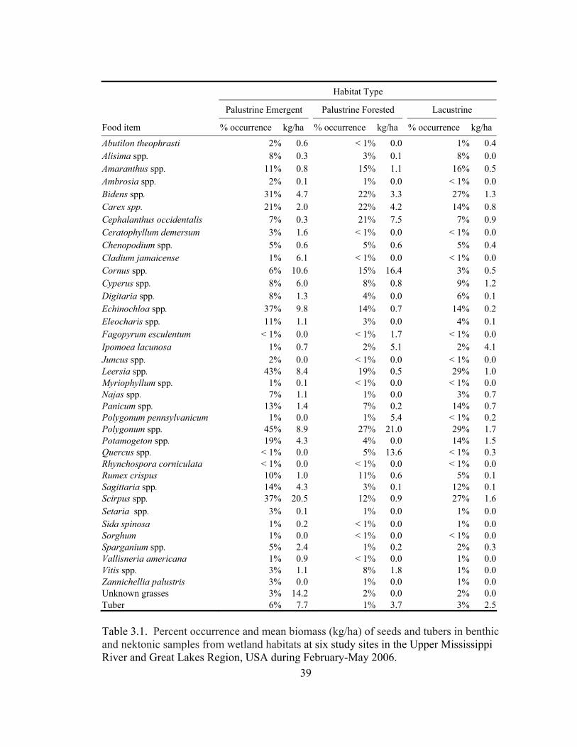
39
Habitat Type
Palustrine Emergent Palustrine Forested Lacustrine
Food item % occurrence kg/ha % occurrence kg/ha % occurrence kg/ha
Abutilon theophrasti 2% 0.6 < 1% 0.0 1% 0.4Alisima spp. 8% 0.3 3% 0.1 8% 0.0Amaranthus spp. 11% 0.8 15% 1.1 16% 0.5Ambrosia spp. 2% 0.1 1% 0.0 < 1% 0.0Bidens spp. 31% 4.7 22% 3.3 27% 1.3Carex spp. 21% 2.0 22% 4.2 14% 0.8Cephalanthus occidentalis 7% 0.3 21% 7.5 7% 0.9Ceratophyllum demersum 3% 1.6 < 1% 0.0 < 1% 0.0Chenopodium spp. 5% 0.6 5% 0.6 5% 0.4Cladium jamaicense 1% 6.1 < 1% 0.0 < 1% 0.0Cornus spp. 6% 10.6 15% 16.4 3% 0.5Cyperus spp. 8% 6.0 8% 0.8 9% 1.2Digitaria spp. 8% 1.3 4% 0.0 6% 0.1Echinochloa spp. 37% 9.8 14% 0.7 14% 0.2Eleocharis spp. 11% 1.1 3% 0.0 4% 0.1Fagopyrum esculentum < 1% 0.0 < 1% 1.7 < 1% 0.0Ipomoea lacunosa 1% 0.7 2% 5.1 2% 4.1Juncus spp. 2% 0.0 < 1% 0.0 < 1% 0.0Leersia spp. 43% 8.4 19% 0.5 29% 1.0Myriophyllum spp. 1% 0.1 < 1% 0.0 < 1% 0.0Najas spp. 7% 1.1 1% 0.0 3% 0.7Panicum spp. 13% 1.4 7% 0.2 14% 0.7Polygonum pennsylvanicum 1% 0.0 1% 5.4 < 1% 0.2Polygonum spp. 45% 8.9 27% 21.0 29% 1.7Potamogeton spp. 19% 4.3 4% 0.0 14% 1.5Quercus spp. < 1% 0.0 5% 13.6 < 1% 0.3Rhynchospora corniculata < 1% 0.0 < 1% 0.0 < 1% 0.0Rumex crispus 10% 1.0 11% 0.6 5% 0.1Sagittaria spp. 14% 4.3 3% 0.1 12% 0.1Scirpus spp. 37% 20.5 12% 0.9 27% 1.6Setaria spp. 3% 0.1 1% 0.0 1% 0.0Sida spinosa 1% 0.2 < 1% 0.0 1% 0.0Sorghum 1% 0.0 < 1% 0.0 < 1% 0.0Sparganium spp. 5% 2.4 1% 0.2 2% 0.3Vallisneria americana 1% 0.9 < 1% 0.0 1% 0.0Vitis spp. 3% 1.1 8% 1.8 1% 0.0Zannichellia palustris 3% 0.0 1% 0.0 1% 0.0Unknown grasses 3% 14.2 2% 0.0 2% 0.0Tuber 6% 7.7 1% 3.7 3% 2.5 Table 3.1. Percent occurrence and mean biomass (kg/ha) of seeds and tubers in benthic and nektonic samples from wetland habitats at six study sites in the Upper Mississippi River and Great Lakes Region, USA during February-May 2006.
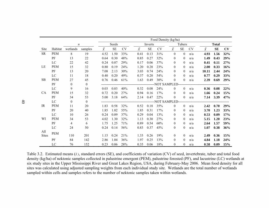
Food Density (kg/ha) n Seeds Inverts Tubers Total Site Habitat wetlands samples x⎯
SE CV x⎯ SE CV x⎯ SE CV x⎯ SE CV SR PEM 8 19 4.52 1.50 33% 0.41 0.13 31% 0 0 n/a 4.93 1.56 32% PF 13 22 0.64 0.30 48% 0.85 0.27 32% 0 0 n/a 1.49 0.43 29% LC 22 42 0.24 0.07 29% 0.17 0.06 37% 0 0 n/a 0.41 0.11 27% LE PEM 15 32 0.80 0.19 24% 1.20 0.28 23% 0 0 n/a 2.00 0.33 16% PF 13 20 7.08 2.13 30% 3.03 0.74 24% 0 0 n/a 10.11 2.44 24% LC 11 18 0.40 0.20 49% 0.37 0.20 54% 0 0 n/a 0.77 0.29 33% SB PEM 27 45 0.76 0.46 61% 1.63 0.49 30% 0 0 n/a 2.39 0.69 29% PF 0 0 -----------------------------------------------NOT SAMPLED--------------------------------------------- LC 9 16 0.03 0.03 40% 0.32 0.08 24% 0 0 n/a 0.36 0.08 22% CA PEM 15 32 0.72 0.20 27% 0.94 0.16 17% 0 0 n/a 1.66 0.24 15% PF 34 53 5.00 3.18 64% 2.14 0.47 22% 0 0 n/a 7.14 3.39 47% LC 0 0 -----------------------------------------------NOT SAMPLED--------------------------------------------- IR PEM 11 20 1.83 0.58 32% 0.52 0.18 35% 0 0 n/a 2.42 0.70 29% PF 20 40 1.85 1.02 55% 1.85 0.31 17% 0 0 n/a 3.70 1.23 33% LC 10 26 0.24 0.09 37% 0.29 0.04 13% 0 0 n/a 0.53 0.09 17% WI PEM 34 53 4.02 1.30 32% 1.13 0.30 27% 0 0 n/a 5.15 1.20 23% PF 4 6 1.75 1.25 71% 0.89 0.54 60% 0 0 n/a 2.64 1.57 59% LC 24 50 0.24 0.14 56% 0.83 0.37 45% 0 0 n/a 1.07 0.38 36% All Sites PEM 110 201 1.15 0.24 21% 1.33 0.26 19% 0 0 n/a 2.49 0.36 15% PF 84 142 2.86 1.04 36% 1.97 0.25 13% 0 0 n/a 4.84 1.18 24% LC 76 152 0.23 0.06 28% 0.35 0.06 18% 0 0 n/a 0.58 0.09 15%
Table 3.2. Estimated means (x⎯ ), standard errors (SE), and coefficients of variation (CV) of seed, invertebrate, tuber and total food density (kg/ha) of nektonic samples collected in palustrine emergent (PEM), palustrine forested (PF), and lacustrine (LC) wetlands at six study sites in the Upper Mississippi River and Great Lakes Region, USA, during February-May 2006. Mean food density for all sites was calculated using adjusted sampling weights from each individual study site. Wetlands are the total number of wetlands sampled within cells and samples refers to the number of nektonic samples taken within wetlands.
40
40

41
greatest at the Lake Erie marshes study site in PF wetlands, representing 7.08 kg/ha and
3.03 kg/ha respectively.
Benthic Food Biomass
I sampled 111 PEM wetlands, 87 PF wetlands and 76 LC wetlands across all sites
(Table 3.3). Marginal plots identified four datum points as having influential weights on
the final mean of within-site estimates; five datum points were influential on among-site
estimates. Therefore, I performed analyses with adjusted weights. Total food density
was greatest in PEM wetlands and ranged from 255 kg/ha at the Scioto River site to 170
kg/ha at the Illinois River site (Table 3.3). Within study sites, CVs were mostly greater
than my desired level of precision (CV ≤ 15%); however, for the total food density
combined sites the CVs for LC estimates were the only ones to exceed CV of 15%
(Table 3.3). Seed density was greatest at the Wisconsin study site in PEM wetlands (212
kg/ha), while invertebrate density was greatest at the Saginaw Bay study site in PEM
wetlands (159 kg/ha). Tubers did not contribute substantially to total food biomass but
was greatest at the Illinois River site in PEM wetlands (84 kg/ha; Table 3.3).
Invertebrate foods
Error variances of invertebrate food density were constant and were linearly
related to explanatory variables as revealed in residual plots. The dispersion parameter of
the full model was 2.65, indicating a high amount of autocorrelation, so I used QAIC that
corrected for over-dispersion and penalized models with more parameters (Burnham and
Anderson 1998). The model containing wetland system was the top approximating
model explaining variation in invertebrate food density (ω 1 = 0.310; Table 3.4).

42
Palustrine emergent wetlands averaged 24.5% more invertebrate food density than
lacustrine wetlands (Figure 3.1). I considered the additive model containing wetland

Food Density (kg/ha) N Seeds Inverts Tubers Total Site Habitat wetlands samples x⎯
SE CV x⎯ SE CV x⎯ SE CV x⎯ SE CV SR PEM 10 23 210 88 42% 43 12 28% 2 1 74% 255 89 35% PF 14 24 65 32 49% 11 2 14% 0 0 n/a 76 32 42% LC 20 42 28 17 62% 26 17 64% 0 0 n/a 54 23 43% LE PEM 14 30 211 65 31% 22 6 28% 0 0 n/a 233 68 29% PF 15 24 194 68 35% 23 4 17% 0 0 n/a 217 68 31% LC 9 16 25 12 49% 7 2 23% 0 0 n/a 32 12 38% SB PEM 27 43 67 20 30% 159 67 42% 0 0 61% 227 70 31% PF 0 0 -----------------------------------------------NOT SAMPLED--------------------------------------------- LC 10 17 3 1 45% 3 1 25% 0 0 n/a 6 1 23% CA PEM 15 39 83 22 26% 60 22 37% 46 28 60% 190 48 25% PF 33 51 78 33 43% 27 6 22% 0 0 n/a 105 34 32% LC 0 0 -----------------------------------------------NOT SAMPLED--------------------------------------------- IR PEM 11 19 78 21 27% 8 3 33% 84 78 93% 170 98 58% PF 20 41 72 17 24% 26 6 24% 5 5 98% 103 19 18% LC 10 27 30 13 44% 39 16 40% 6 6 94% 75 26 35% WI PEM 34 55 212 42 20% 40 21 54% 2 2 89% 254 54 21% PF 5 8 186 95 51% 12 8 70% 0 0 n/a 198 100 50% LC 24 54 123 20 16% 123 36 29% 0 0 87% 247 43 18% All PEM 111 209 118 21 17% 68 15 22% 8 4 56% 194 25 13% PF 87 149 82 15 18% 26 4 17% 4 4 97% 112 16 14% LC 73 156 19 5 25% 18 5 28% 3 2 96% 40 8 20%
Table 3.3. Estimated means(x⎯ ), standard errors (SE), and coefficients of variation (CV) of seed, invertebrate, tuber and total food density (kg/ha) of benthic samples collected in palustrine emergent (PEM), palustrine forested (PF), and lacustrine (LC) wetlands at six study sites in the Upper Mississippi River and Great Lakes Region, USA, during February-May 2006. Mean food density for all sites was calculated using adjusted sampling weights from each individual study site. Wetlands are the total number of wetlands sampled within cells and samples refers to the number of benthic samples taken within wetlands.
43
43

44
Model K QAIC ∆QAIC ω i R2 System 3 770.7 0.0 0.310 0.02 System + Period 4 772.0 1.3 0.163 0.02 System + Zone 4 772.7 2.0 0.116 0.02 Period 2 773.1 2.4 0.094 0.00 Zone 2 773.8 3.0 0.068 0.00 System * Period 6 773.9 3.2 0.064 0.03 System + Cover 7 774.0 3.2 0.061 0.04 Site 6 775.3 4.6 0.031 0.02 System* Zone 6 776.2 5.5 0.020 0.02 Site + Period 7 776.3 5.6 0.019 0.03 System + Site 8 776.4 5.7 0.018 0.03 Cover 5 776.7 5.9 0.016 0.01 Site +System +Period 9 777.5 6.8 0.010 0.04 Site* System 18 778.4 7.7 0.007 0.10 Site * Period 11 781.8 11.1 0.001 0.03 System* Cover 15 786.0 15.3 0.000 0.04 Site * System * Period 37 800.8 30.1 0.000 0.13 null 1 982.5 211.8 0.000 n/a
a SITE = study site; SYSTEM = wetland system (i.e., palustrine emergent, palustrine forested, lacustrine); PERIOD = sampling period; COVER = vegetation cover type; ZONE = sampling zone (i.e., shallow vs. deep). Table 3.4. Candidate models explaining variation in benthic invertebrate food density (kg/ha) sampled in wetlands at six sites in the Upper Mississippi River and Great Lakes Region, USA during February-May 2006. Models are ranked by Quasi-Akaike’s Information Criterion (QAIC). Also included are the number of estimable parameters (K), model weight (ω i), and proportion of variance accounted for (R2).

system and sampling period (ω 1 = 0.163) competitive since it was within 2 ∆QAIC units
of the top model. Invertebrate density increased from early to late sampling period
(Figure 3.2).
Plant Foods
Error variances of plant food density were constant and were linearly related to
explanatory variables as revealed in residual plots. The dispersion parameter of the full
model was 4.01, indicating a high amount of autocorrelation, so I used QAIC that
corrected for over-dispersion and penalized models with more parameters (Burnham and
Anderson 1998).
The top approximating model explaining variation in plant food density was the
additive model containing wetland system and study site (ω 1 = 0.506; Table 3.5).
Palustrine emergent wetlands averaged 41.5% more plant food density than lacustrine
wetlands (Figure 3.1). The east-central Wisconsin site had the greatest food density
(Figure 3.3). The next closest model, which I considered competitive since it was within
2 ∆QAIC units, was the additive model of wetland system, study site, and sampling
period (ω 1 = 0.224). Similar to invertebrate density, plant food density also increased
between early and late sampling periods (Figure 3.2).
Cropland Food Biomass
I adjusted weights of four samples from the east-central Wisconsin study site for
the within-site estimates. I adjusted weights for one sample from the east-central
Wisconsin site and one sample from the Lake Erie Marshes site for the among-site
estimates.

0
0.5
1
1.5
2
2.5
3
3.5
4
4.5
Palustrine emergent Palustrine forested Lacustrine
Log
(kg/
ha)
Seed densityInvertebrate density
Figure 3.1 Seed and invertebrate densities with standard errors in wetland habitat types, pooled across study sites and sampling periods. Samples were obtained in wetland habitats in Upper Mississippi River and Great Lakes Region during February-May 2006.
0
0.5
1
1.5
2
2.5
3
3.5
4
Early Sampling Period Late Sampling Period
Log
(kg/
ha)
Seed densityInvertebrate density
Figure 3.2. Seed and invertebrate densities during early (before arrival of migrating waterfowl) and late(after departure of migrating waterfowl) sampling periods, pooled across study sites and habitat types. Samples were obtained in wetland habitats in Upper Mississippi River and Great Lakes Region during February-May 2006.
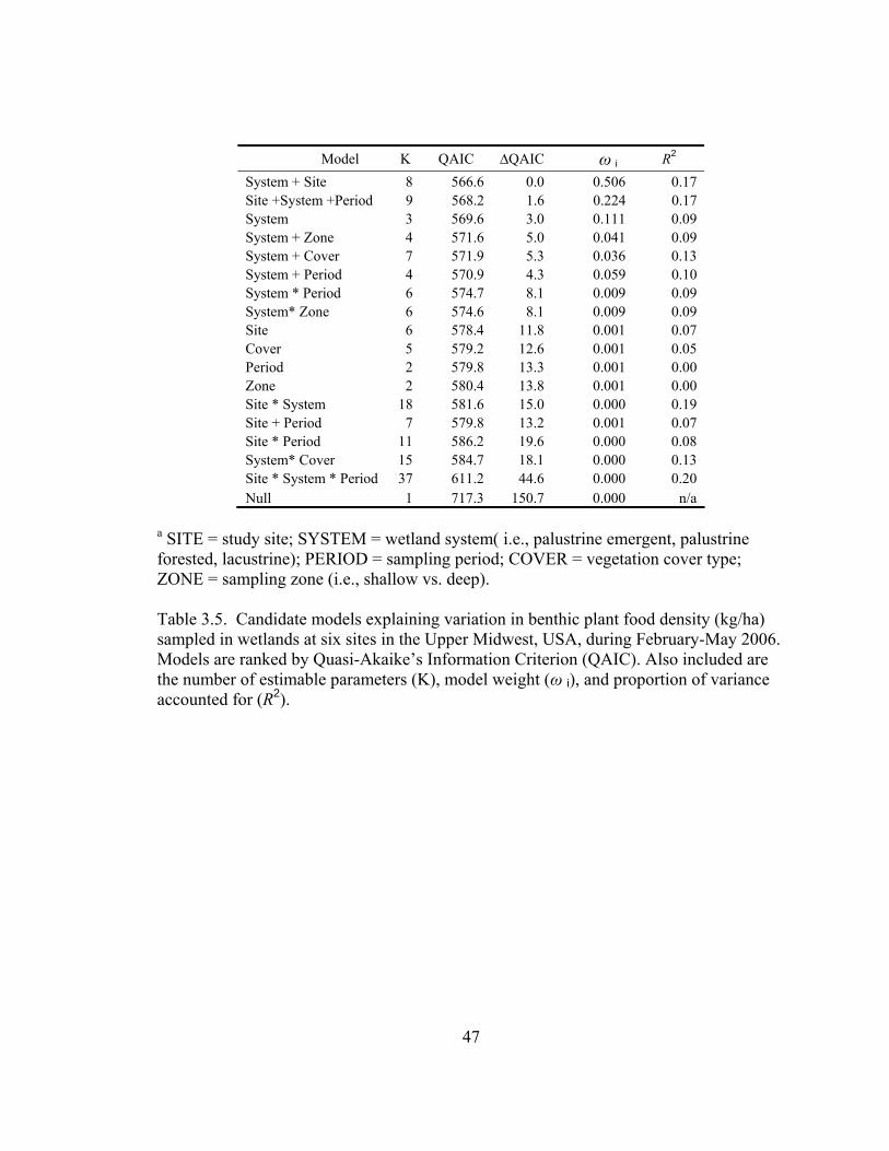
47
Model K QAIC ∆QAIC ω i R2 System + Site 8 566.6 0.0 0.506 0.17 Site +System +Period 9 568.2 1.6 0.224 0.17 System 3 569.6 3.0 0.111 0.09 System + Zone 4 571.6 5.0 0.041 0.09 System + Cover 7 571.9 5.3 0.036 0.13 System + Period 4 570.9 4.3 0.059 0.10 System * Period 6 574.7 8.1 0.009 0.09 System* Zone 6 574.6 8.1 0.009 0.09 Site 6 578.4 11.8 0.001 0.07 Cover 5 579.2 12.6 0.001 0.05 Period 2 579.8 13.3 0.001 0.00 Zone 2 580.4 13.8 0.001 0.00 Site * System 18 581.6 15.0 0.000 0.19 Site + Period 7 579.8 13.2 0.001 0.07 Site * Period 11 586.2 19.6 0.000 0.08 System* Cover 15 584.7 18.1 0.000 0.13 Site * System * Period 37 611.2 44.6 0.000 0.20 Null 1 717.3 150.7 0.000 n/a
a SITE = study site; SYSTEM = wetland system( i.e., palustrine emergent, palustrine forested, lacustrine); PERIOD = sampling period; COVER = vegetation cover type; ZONE = sampling zone (i.e., shallow vs. deep). Table 3.5. Candidate models explaining variation in benthic plant food density (kg/ha) sampled in wetlands at six sites in the Upper Midwest, USA, during February-May 2006. Models are ranked by Quasi-Akaike’s Information Criterion (QAIC). Also included are the number of estimable parameters (K), model weight (ω i), and proportion of variance accounted for (R2).
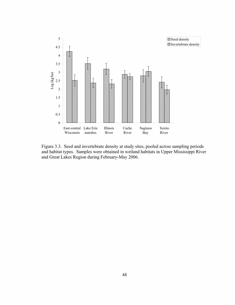
0
0.5
1
1.5
2
2.5
3
3.5
4
4.5
5
East-centralWisconsin
Lake Eriemarshes
IllinoisRiver
CacheRiver
SaginawBay
SciotoRiver
Log
(kg/
ha)
Seed densityInvertebrate density
Figure 3.3. Seed and invertebrate density at study sites, pooled across sampling periods and habitat types. Samples were obtained in wetland habitats in Upper Mississippi River and Great Lakes Region during February-May 2006.
48

49
I obtained 83 samples from corn fields and 31 from soybean fields across all sites
(Table 3.6). Total food density in croplands varied from 223 kg/ha at the Illinois River
site to 17 kg/ha at the Lake Erie site (Table 3.6) for the within site estimates. Biomass
density from cornfields always exceeded soybean fields (Table 3.6). All estimates from
all sites exceeded the desired CV of 15%.
Relative biomass, Plant versus. Invertebrate Foods
Percent invertebrate contribution from benthic samples differed by study site (F
(5,505) = 5.06, P < 0.001) and wetland system (F (2,505) = 6.79, P = 0.001). I did not detect
a difference between sampling periods (F (1,505) = 0.65, P = 0.419). Benthic invertebrates
comprised the highest mean percentage (79%) of total biomass in lacustrine habitats at
the Saginaw Bay study site during the late sampling period, while palustrine emergent
wetlands at the Illinois River site during the late sampling period comprised the least
(15%; Figure 3.4).
Percent invertebrate contribution from nektonic samples differed by study site (F
(5,487) = 9.04, P < 0.001), wetland system (F (2,487) = 8.52, P < 0.001) and sampling period
(F (1,487) = 5.79, P = 0.016). Lacustrine wetlands at Saginaw Bay during the late sampling
period comprised the highest mean percentage (80%) of total biomass, while palustrine
forested wetlands in Wisconsin during the early sampling period made up the least (11%,
Figure 3.5).
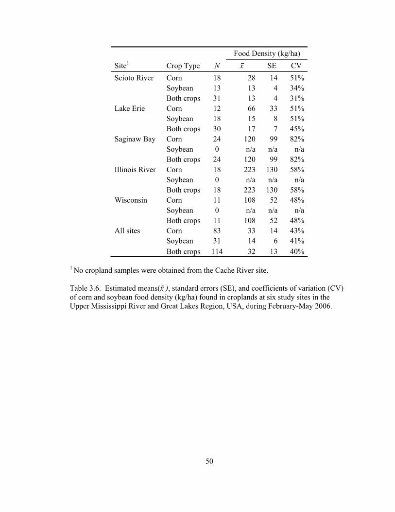
50
Food Density (kg/ha) Site1 Crop Type N x⎯ SE CV Scioto River Corn 18 28 14 51% Soybean 13 13 4 34% Both crops 31 13 4 31% Lake Erie Corn 12 66 33 51% Soybean 18 15 8 51% Both crops 30 17 7 45% Saginaw Bay Corn 24 120 99 82% Soybean 0 n/a n/a n/a Both crops 24 120 99 82% Illinois River Corn 18 223 130 58% Soybean 0 n/a n/a n/a Both crops 18 223 130 58% Wisconsin Corn 11 108 52 48% Soybean 0 n/a n/a n/a Both crops 11 108 52 48% All sites Corn 83 33 14 43% Soybean 31 14 6 41% Both crops 114 32 13 40%
1 No cropland samples were obtained from the Cache River site.
Table 3.6. Estimated means(x⎯ ), standard errors (SE), and coefficients of variation (CV) of corn and soybean food density (kg/ha) found in croplands at six study sites in the Upper Mississippi River and Great Lakes Region, USA, during February-May 2006.

0%
10%
20%
30%
40%
50%
60%
70%
80%
90%
100%
Early Late Early Late Early Late Early Late Early Late Early Late
Cache River Illinois River Lake Erie Saginaw Bay Scioto River Wisconsin
Palustrine Emergent
Mea
n %
Inve
rtebr
ates
InvertebratesSeeds and Tubers
A
Figure 3.4. Mean % invertebrates of total benthic biomass (kg/ha) in palustrine emergent (A), palustrine forested (B) and lacustrine (C) wetlands sampled in the Upper Mississippi River and Great Lakes Region during February-May 2006. Palustrine forested wetlands were not sampled at Saginaw Bay. Lacustrine wetlands were not sampled at the Cache River.
continued
51
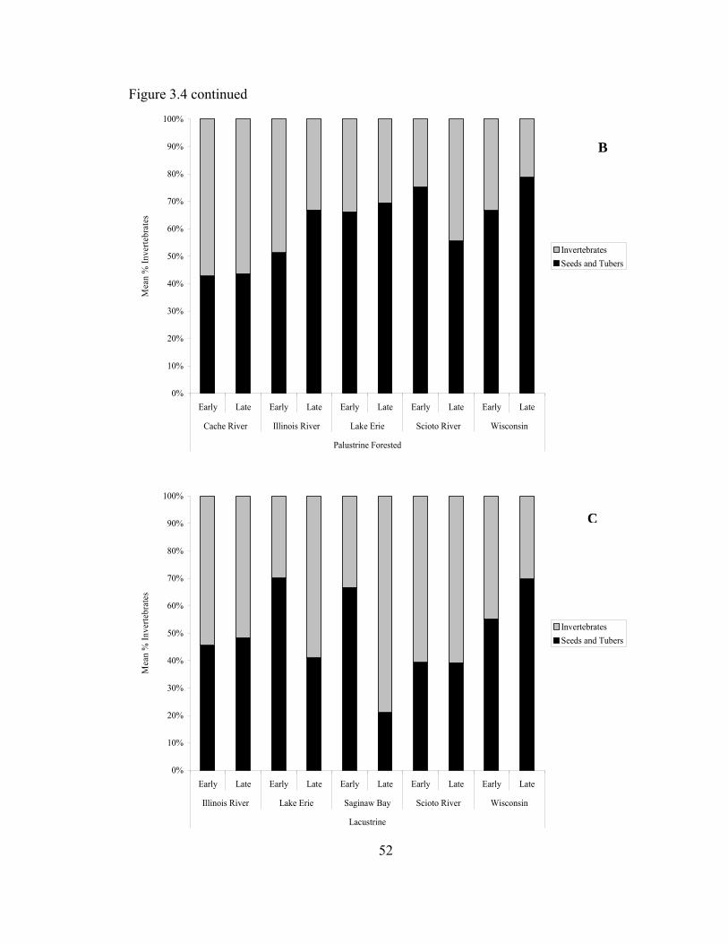
Figure 3.4 continued
0%
10%
20%
30%
40%
50%
60%
70%
80%
90%
100%
Early Late Early Late Early Late Early Late Early Late
Cache River Illinois River Lake Erie Scioto River Wisconsin
Palustrine Forested
Mea
n %
Inve
rtebr
ates
InvertebratesSeeds and Tubers
B
52
0%
10%
20%
30%
40%
50%
60%
70%
80%
90%
100%
Early Late Early Late Early Late Early Late Early Late
Illinois River Lake Erie Saginaw Bay Scioto River Wisconsin
Lacustrine
Mea
n %
Inve
rtebr
ates
InvertebratesSeeds and Tubers
C
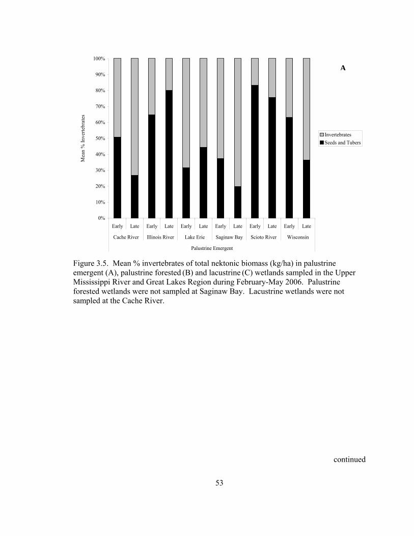
0%
10%
20%
30%
40%
50%
60%
70%
80%
90%
100%
Early Late Early Late Early Late Early Late Early Late Early Late
Cache River Illinois River Lake Erie Saginaw Bay Scioto River Wisconsin
Palustrine Emergent
Mea
n %
Inve
rtebr
ates
InvertebratesSeeds and Tubers
A
Figure 3.5. Mean % invertebrates of total nektonic biomass (kg/ha) in palustrine emergent (A), palustrine forested (B) and lacustrine (C) wetlands sampled in the Upper Mississippi River and Great Lakes Region during February-May 2006. Palustrine forested wetlands were not sampled at Saginaw Bay. Lacustrine wetlands were not sampled at the Cache River.
continued
53
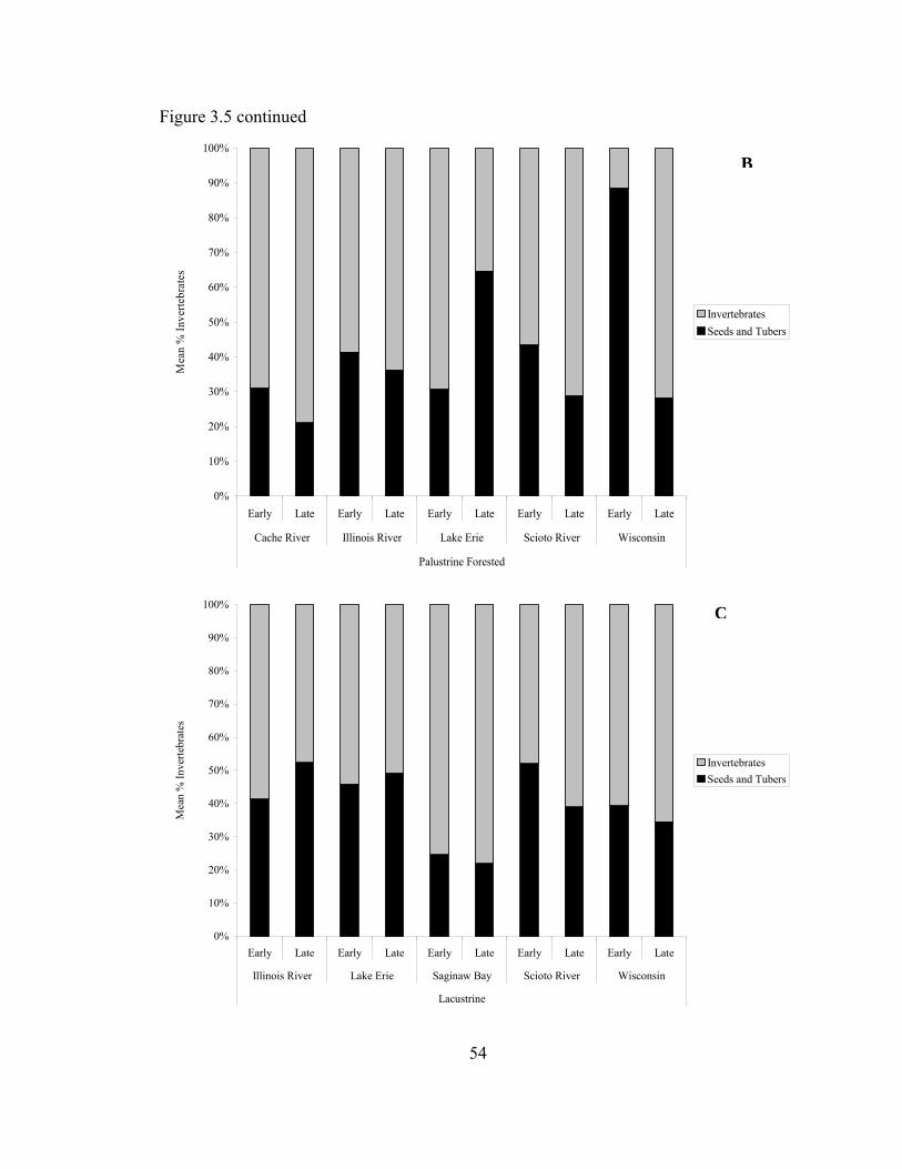
Figure 3.5 continued
0%
10%
20%
30%
40%
50%
60%
70%
80%
90%
100%
Early Late Early Late Early Late Early Late Early Late
Cache River Illinois River Lake Erie Scioto River Wisconsin
Palustrine Forested
Mea
n %
Inve
rtebr
ates
InvertebratesSeeds and Tubers
B
0%
10%
20%
30%
40%
50%
60%
70%
80%
90%
100%
Early Late Early Late Early Late Early Late Early Late
Illinois River Lake Erie Saginaw Bay Scioto River Wisconsin
Lacustrine
Mea
n %
Inve
rtebr
ates
InvertebratesSeeds and Tubers
C
54
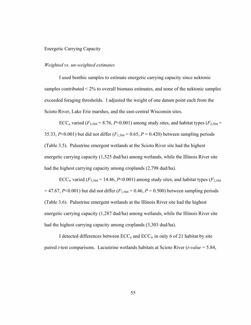
55
Energetic Carrying Capacity
Weighted vs. un-weighted estimates
I used benthic samples to estimate energetic carrying capacity since nektonic
samples contributed < 2% to overall biomass estimates, and none of the nektonic samples
exceeded foraging thresholds. I adjusted the weight of one datum point each from the
Scioto River, Lake Erie marshes, and the east-central Wisconsin sites.
ECCu varied (F5,504 = 8.76, P<0.001) among study sites, and habitat types (F2,504 =
35.33, P<0.001) but did not differ (F1,504 = 0.65, P = 0.420) between sampling periods
(Table 3.5). Palustrine emergent wetlands at the Scioto River site had the highest
energetic carrying capacity (1,525 dud/ha) among wetlands, while the Illinois River site
had the highest carrying capacity among croplands (2,798 dud/ha).
ECCw varied (F5,504 = 14.46, P<0.001) among study sites, and habitat types (F2,504
= 47.67, P<0.001) but did not differ (F1,504 = 0.46, P = 0.500) between sampling periods
(Table 3.6). Palustrine emergent wetlands at the Illinois River site had the highest
energetic carrying capacity (1,287 dud/ha) among wetlands, while the Illinois River site
had the highest carrying capacity among croplands (3,303 dud/ha).
I detected differences between ECCu and ECCw in only 6 of 21 habitat by site
paired t-test comparisons. Lacustrine wetlands habitats at Scioto River (t-value = 5.84,
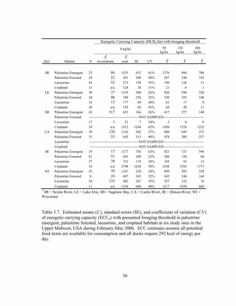
56
Energetic Carrying Capacity (DUDu/ha) with foraging threshold
0 kg/ha 50
kg/ha 130
kg/ha 280
kg/ha
Site1 Habitat N x⎯
invertebrate x⎯
total SE CV x⎯ x⎯ x⎯
SR Palustrine Emergent 23 86 1525 632 41% 1276 994 708 Palustrine Forested 24 22 431 208 48% 287 246 185 Lacustrine 42 52 272 150 55% 190 126 31 Cropland 31 n/a 124 38 31% 21 6 1
LE Palustrine Emergent 30 37 1155 300 26% 920 596 320 Palustrine Forested 24 46 749 236 32% 520 355 140 Lacustrine 16 13 177 84 48% 81 17 8 Cropland 30 n/a 159 69 43% 68 20 11
SB Palustrine Emergent 43 317 633 166 26% 417 277 140 Palustrine Forested -------------------------------------------NOT SAMPLED----------------------------------- Lacustrine 17 5 21 7 34% 2 0 0 Cropland 24 n/a 1512 1244 82% 1450 1376 1252
CA Palustrine Emergent 39 120 1126 302 27% 880 645 373 Palustrine Forested 51 53 645 313 49% 478 389 257 Lacustrine -------------------------------------------NOT SAMPLED----------------------------------- Cropland -------------------------------------------NOT SAMPLED-----------------------------------
IR Palustrine Emergent 19 17 1177 736 63% 921 727 596 Palustrine Forested 41 51 456 100 22% 260 158 60 Lacustrine 27 78 312 119 38% 185 93 12 Cropland 18 n/a 2798 1628 58% 2588 2295 1773
WI Palustrine Emergent 55 79 1167 230 20% 899 585 228 Palustrine Forested 8 24 697 363 52% 442 346 164 Lacustrine 54 135 482 267 55% 327 122 10 Cropland 11 n/a 1354 648 48% 1217 1039 668
1 SR = Scioto River, LE = Lake Erie, SB = Saginaw Bay, CA = Cache River, IR = Illinois River, WI = Wisconsin Table 3.7. Estimated means (x⎯ ), standard errors (SE), and coefficients of variation (CV) of energetic carrying capacity (ECCu) with presumed foraging threshold in palustrine emergent, palustrine forested, lacustrine, and cropland habitats at six study sites in the Upper Midwest, USA during February-May 2006. ECC estimates assume all potential food items are available for consumption and all ducks require 292 kcal of energy per day.
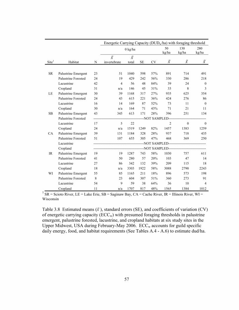
57
Energetic Carrying Capacity (DUDw/ha) with foraging threshold
0 kg/ha
50
kg/ha 130
kg/ha 280
kg/ha
Site1 Habitat N x⎯
invertebrate x⎯
total SE CV x⎯ x⎯ x⎯
SR Palustrine Emergent 23 51 1040 598 57% 891 714 491 Palustrine Forested 24 19 429 242 56% 330 286 218 Lacustrine 42 4 56 48 84% 39 24 0 Cropland 31 n/a 146 45 31% 33 8 3
LE Palustrine Emergent 30 39 1168 317 27% 935 625 354 Palustrine Forested 24 43 615 221 36% 424 276 86 Lacustrine 16 14 169 87 52% 73 11 0 Cropland 30 n/a 164 71 43% 71 21 11
SB Palustrine Emergent 43 345 613 171 28% 396 251 134 Palustrine Forested -------------------------------------------NOT SAMPLED-------------------------------- Lacustrine 17 5 22 2 0 0 Cropland 24 n/a 1519 1249 82% 1457 1383 1259
CA Palustrine Emergent 39 131 1184 328 28% 937 718 435 Palustrine Forested 51 107 655 305 47% 468 369 250 Lacustrine -------------------------------------------NOT SAMPLED-------------------------------- Cropland -------------------------------------------NOT SAMPLED--------------------------------
IR Palustrine Emergent 19 19 1287 743 58% 1030 757 611 Palustrine Forested 41 50 280 57 20% 103 47 14 Lacustrine 27 86 342 132 39% 209 115 18 Cropland 18 n/a 3303 1922 58% 3088 2790 2243
WI Palustrine Emergent 55 85 1165 211 18% 896 573 198 Palustrine Forested 8 23 604 307 51% 360 273 91 Lacustrine 54 9 59 38 64% 36 10 4 Cropland 11 n/a 1707 817 48% 1565 1384 1012
1 SR = Scioto River, LE = Lake Erie, SB = Saginaw Bay, CA = Cache River, IR = Illinois River, WI = Wisconsin Table 3.8 Estimated means (x⎯ ), standard errors (SE), and coefficients of variation (CV) of energetic carrying capacity (ECCw) with presumed foraging thresholds in palustrine emergent, palustrine forested, lacustrine, and cropland habitats at six study sites in the Upper Midwest, USA during February-May 2006. ECCw accounts for guild specific daily energy, food, and habitat requirements (See Tables A.4 - A.6) to estimate dud/ha.
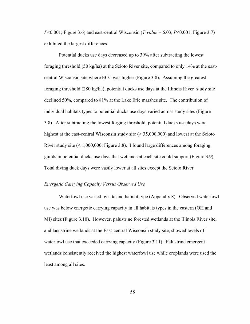
58
P<0.001; Figure 3.6) and east-central Wisconsin (T-value = 6.03, P<0.001; Figure 3.7)
exhibited the largest differences.
Potential ducks use days decreased up to 39% after subtracting the lowest
foraging threshold (50 kg/ha) at the Scioto River site, compared to only 14% at the east-
central Wisconsin site where ECC was higher (Figure 3.8). Assuming the greatest
foraging threshold (280 kg/ha), potential ducks use days at the Illinois River study site
declined 50%, compared to 81% at the Lake Erie marshes site. The contribution of
individual habitats types to potential ducks use days varied across study sites (Figure
3.8). After subtracting the lowest forging threshold, potential ducks use days were
highest at the east-central Wisconsin study site (> 35,000,000) and lowest at the Scioto
River study site (< 1,000,000; Figure 3.8). I found large differences among foraging
guilds in potential ducks use days that wetlands at each site could support (Figure 3.9).
Total diving duck days were vastly lower at all sites except the Scioto River.
Energetic Carrying Capacity Versus Observed Use
Waterfowl use varied by site and habitat type (Appendix 8). Observed waterfowl
use was below energetic carrying capacity in all habitats types in the eastern (OH and
MI) sites (Figure 3.10). However, palustrine forested wetlands at the Illinois River site,
and lacustrine wetlands at the East-central Wisconsin study site, showed levels of
waterfowl use that exceeded carrying capacity (Figure 3.11). Palustrine emergent
wetlands consistently received the highest waterfowl use while croplands were used the
least among all sites.

0
500
1000
1500
2000
2500
3000
PalustrineEmergent
PalustrineForested
Lacustrine Cropland PalustrineEmergent
PalustrineForested
Lacustrine Cropland PalustrineEmergent
Lacustrine Cropland
Scioto River Lake Erie marshes Saginaw Bay
DU
D/h
a
ECCuECCw
*
*59
*
Figure 3.6. Energetic carrying capacity estimates (DUD/ha) +/- standard errors for ECCu and ECCw at the Scioto River, Lake Erie Marshes and Saginaw Bay Study sites in wetland and cropland habitats during February-May 2006. * = significant difference with paired t-test (P < 0.05)

0
1000
2000
3000
4000
5000
6000
PalustrineEmergent
PalustrineForested
PalustrineEmergent
PalustrineForested
Lacustrine Cropland PalustrineEmergent
PalustrineForested
Lacustrine Cropland
Cache River Illinois River East Central Wisconsin
DU
D/h
a ECCuECCw
*60
**
Figure 3.7. Energetic carrying capacity estimates (DUD/ha) +/- standard errors for ECCu and ECCw at the Cache River, Illinois River and East Central Wisconsin Study sites in wetland and cropland habitats during February-May 2006. * = significant difference with paired t-test (P < 0.05)
60

0
5,000,000
10,000,000
15,000,000
20,000,000
25,000,000
30,000,000
35,000,000
40,000,000
45,000,000
none
50 K
g/ha
130
Kg/
ha
300
Kg/
ha
none
50 K
g/ha
130
Kg/
ha
300
Kg/
ha
none
50 K
g/ha
130
Kg/
ha
300
Kg/
ha
none
50 K
g/ha
130
Kg/
ha
300
Kg/
ha
none
50 K
g/ha
130
Kg/
ha
300
Kg/
ha
none
50 K
g/ha
130
Kg/
ha
300
Kg/
ha
Foraging threshold Foraging threshold Foraging threshold Foraging threshold Foraging threshold Foraging threshold
Scioto River Lake Erie Saginaw Bay Cache River Illinois River Wisconsin
Pote
ntia
l Duc
k U
se D
ays
CroplandLacustrineForestedEmergent
61
Figure 3.8. Contribution of cropland, lacustrine, palustrine forested, and palustrine emergent habitats to potential duck use days assuming no foraging threshold (none) and three theoretical thresholds at six study sites in the Upper Mississippi River and Great Lakes Region, USA, during February-May 2006. ECCw estimates (Table 3.8) were multiplied by amount of habitat at a site (Table 1.1) to derive potential duck use days. 61
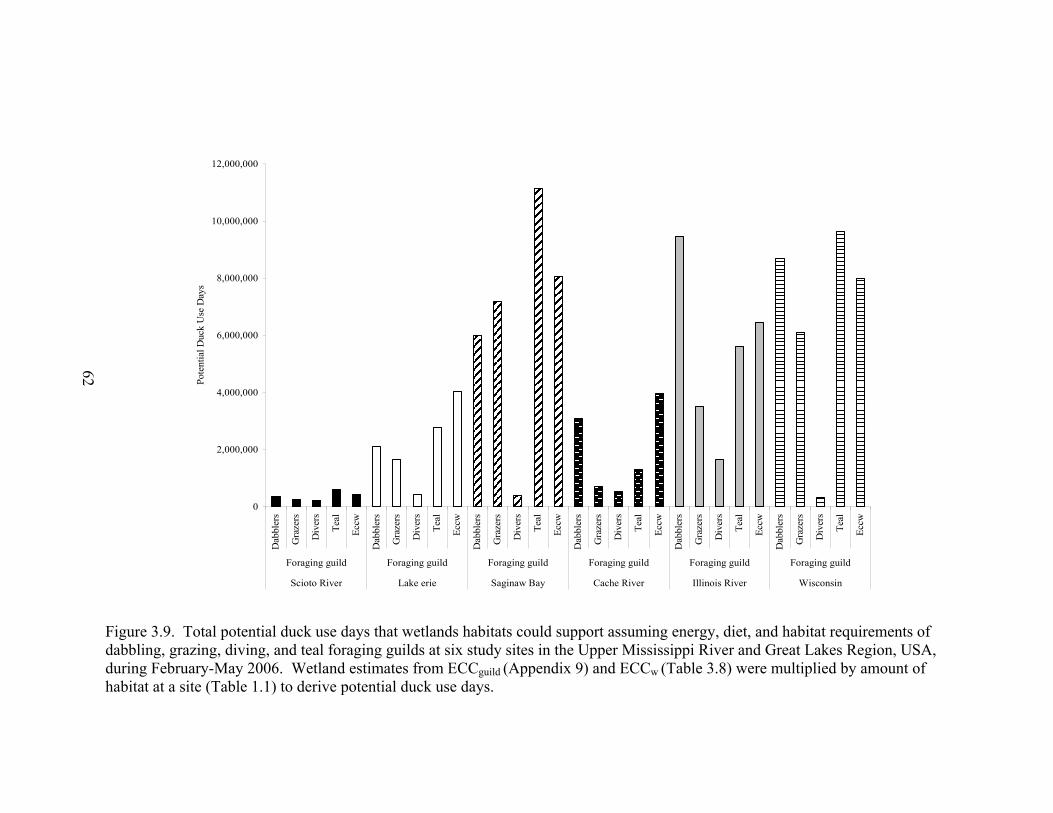
62
0
2,000,000
4,000,000
6,000,000
8,000,000
10,000,000
12,000,000
Dab
bler
s
Gra
zers
Div
ers
Teal
Eccw
Dab
bler
s
Gra
zers
Div
ers
Teal
Eccw
Dab
bler
s
Gra
zers
Div
ers
Teal
Eccw
Dab
bler
s
Gra
zers
Div
ers
Teal
Eccw
Dab
bler
s
Gra
zers
Div
ers
Teal
Eccw
Dab
bler
s
Gra
zers
Div
ers
Teal
Eccw
Foraging guild Foraging guild Foraging guild Foraging guild Foraging guild Foraging guild
Scioto River Lake erie Saginaw Bay Cache River Illinois River Wisconsin
Pote
ntia
l Duc
k U
se D
ays
Figure 3.9. Total potential duck use days that wetlands habitats could support assuming energy, diet, and habitat requirements of dabbling, grazing, diving, and teal foraging guilds at six study sites in the Upper Mississippi River and Great Lakes Region, USA, during February-May 2006. Wetland estimates from ECCguild (Appendix 9) and ECCw (Table 3.8) were multiplied by amount of habitat at a site (Table 1.1) to derive potential duck use days.
62
0
200
400
600
800
1,000
1,200
1,400
1,600
1,800
PalustrineEmergent
Palustrine Forested Lacustrine Cropland
Scioto River
DU
D/h
a
Carrying CapacityObserved Use
Foraging Threshold*
A
0
200
400
600
800
1,000
1,200
1,400
1,600
Palustrine Emergent Palustrine Forested Lacustrine Cropland
Lake Erie Marshes
DU
D/h
a
Carry CapacityObserved Use
Foraging Threshold*
Figure 3.10. Energetic carrying capacity (weighted) +/- standard errors and mean observed waterfowl use/ha on palustrine emergent, palustrine forested, and lacustrine wetlands and croplands at Scioto River (A), Lake Erie (B) and Saginaw Bay (C) study sites during February-May 2006. Energetic foraging threshold is equivalent to 50 kg/ha food density.
B
continued 63
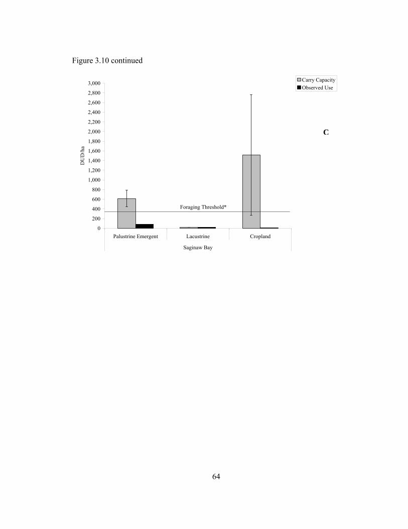
Figure 3.10 continued
0
200
400
600
800
1,000
1,200
1,400
1,600
1,800
2,000
2,200
2,400
2,600
2,800
3,000
Palustrine Emergent Lacustrine Cropland
Saginaw Bay
DU
D/h
aCarry CapacityObserved Use
Foraging Threshold*
C
64

0
200
400
600
800
1,000
1,200
1,400
1,600
Palustrine Emergent Palustrine Forested Cropland
Cache River
DU
D/h
a
Carrying CapacityObserved Use
Foraging Threshold*
0200400600800
1,0001,2001,4001,6001,8002,0002,2002,4002,6002,8003,0003,2003,4003,6003,8004,0004,2004,4004,6004,8005,000
Palustrine Emergent Palustrine Forested Lacustrine Cropland
Illinois River
DU
D/h
a
Carry CapacityObserved Use
Foraging Threshold*
A
B
Figure 3.11. Energetic carrying capacity (weighted) +/- standard errors and mean observed waterfowl use/ha on palustrine emergent, palustrine forested, and lacustrine wetlands and croplands at Cache River (A), Illinois River (B) and East-central Wisconsin (C) study sites during February-May 2006. Energetic foraging threshold is equivalent to 50 kg/ha food density.
continued 65

Figure 3.11 continued
0
200
400
600
800
1,000
1,200
1,400
1,600
1,800
2,000
2,200
2,400
2,600
Palustrine Emergent Palustrine Forested Lacustrine Cropland
Wisconsin
DU
D/h
aCarry capacityObserved Use
Foraging Threshold*
C
66
67
CHAPTER 4
DISCUSSION
In contrast to other NAWMP Joint Venture regions such as the Mississippi
Alluvial Valley and the Central Valley of California, the UMRGLR contains a wide
diversity of wetland types (Bookhout et al. 1989). Therefore, an attempt to quantify and
compare food abundance among habitat types in the region has been challenging.
Conservation planners need reliable food abundance estimates for croplands, marshes,
natural lakes, rivers, impoundments, and riparian forests to effectively anticipate
energetic and nutritional needs of spring-migrating waterfowl. These habitat types
individually and collectively contribute to the total habitat resource that supports spring-
migrating in the UMRGLR. My results provide a basis for understanding variation in
food resource abundance along latitudinal and longitudinal gradients in the region.
Northern sites (i.e., Saginaw Bay and east-central Wisconsin) tended to have more
food biomass in lacustrine, palustrine, forested and cropland habitats than southern sites
(i.e., Scioto River and Cache River). Western sites tended to have more food biomass
density in lacustrine and cropland habitats, compared to the eastern sites. Total food
density varied among sites and habitat types. Palustrine emergent wetlands consistently
had the highest food density (kg/ha) across study sites, followed by palustrine forested
68
wetlands, lacustrine wetlands, and finally croplands. Large differences among similar
habitat types suggest regional differences in site factors influence food abundance.
Plant seeds accounted for the majority of food biomass in all wetland types, but
species composition and biomass differed among wetland types. Plant food was
concentrated primarily on or within the substrate of wetlands, contributing >98% of total
food biomass. Similar to my results, Bartonek and Hickey (1969) reported few seeds
(<1% total food) in the water column and Baldassarre (1980) further corroborated this
pattern by finding the majority (>85%) of seeds in benthic samples.
My estimates of biomass density were generally similar to other estimates;
however, few studies of this type have been conducted during spring (Table 4.1).
Variability in estimates among studies likely resulted from site-specific influences or
different sampling and estimation methods. My benthic sampling method quantified
biomass density of food in the top 10cm of the substrate. The ability of waterfowl to
access food in the substrate likely differs among species. In fact, numerous studies have
demonstrated substantial differences in niche overlap in terms of foraging depth (Nudds
1983). Canvasbacks are known to consume sago pondweed (Potamogeton pectinatus)
tubers up to 20 cm below the substrate surface (Anderson and Low 1976). My estimates
of biomass in the substrate of wetlands were similar to Naylor (2002) and Dibona (2008)
who also sampled the top 10cm of the substrate during spring. However, my estimates
were substantially higher than Brasher et al. (2007) who sampled passive- and active-
managed wetlands in central and northern Ohio during springs 2000 – 2002. Brasher et
al. (2007) sampled only to the surface of the substrate using a stove-pipe sampler. Thus,
a likely reason why my estimates were higher is my sampling technique quantified
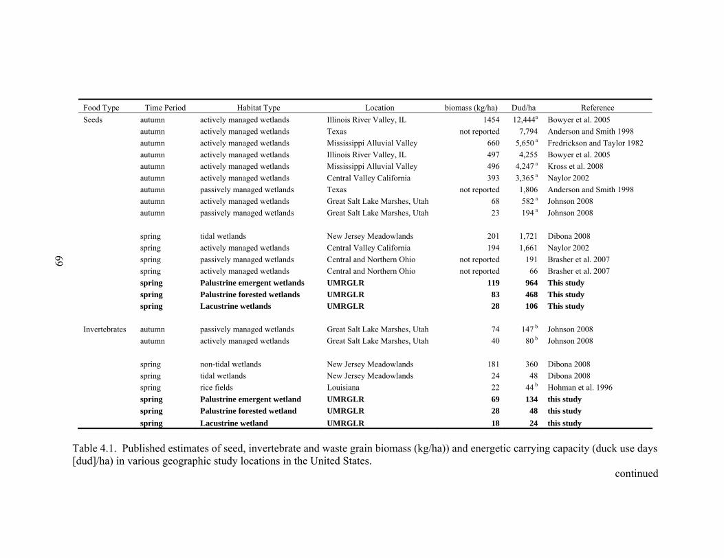
Food Type Time Period Habitat Type Location biomass (kg/ha) Dud/ha Reference Seeds autumn actively managed wetlands Illinois River Valley, IL 1454 12,444a Bowyer et al. 2005 autumn actively managed wetlands Texas not reported 7,794 Anderson and Smith 1998 autumn actively managed wetlands Mississippi Alluvial Valley 660 5,650 a Fredrickson and Taylor 1982 autumn actively managed wetlands Illinois River Valley, IL 497 4,255 Bowyer et al. 2005 autumn actively managed wetlands Mississippi Alluvial Valley 496 4,247 a Kross et al. 2008 autumn actively managed wetlands Central Valley California 393 3,365 a Naylor 2002 autumn passively managed wetlands Texas not reported 1,806 Anderson and Smith 1998 autumn actively managed wetlands Great Salt Lake Marshes, Utah 68 582 a Johnson 2008 autumn passively managed wetlands Great Salt Lake Marshes, Utah 23 194 a Johnson 2008 spring tidal wetlands New Jersey Meadowlands 201 1,721 Dibona 2008 spring actively managed wetlands Central Valley California 194 1,661 Naylor 2002 spring passively managed wetlands Central and Northern Ohio not reported 191
69 Brasher et al. 2007 spring actively managed wetlands Central and Northern Ohio not reported 66 Brasher et al. 2007 spring Palustrine emergent wetlands UMRGLR 119 964 This study spring Palustrine forested wetlands UMRGLR 83 468 This study spring Lacustrine wetlands UMRGLR 28 106 This study Invertebrates autumn passively managed wetlands Great Salt Lake Marshes, Utah 74 147 b Johnson 2008 autumn actively managed wetlands Great Salt Lake Marshes, Utah 40 80 b Johnson 2008 spring non-tidal wetlands New Jersey Meadowlands 181 360 Dibona 2008 spring tidal wetlands New Jersey Meadowlands 24 48 Dibona 2008 spring rice fields Louisiana 22 44 b Hohman et al. 1996 spring Palustrine emergent wetland UMRGLR 69 134 this study spring Palustrine forested wetland UMRGLR 28 48 this study spring Lacustrine wetland UMRGLR 18 24 this study
Table 4.1. Published estimates of seed, invertebrate and waste grain biomass (kg/ha)) and energetic carrying capacity (duck use days [dud]/ha) in various geographic study locations in the United States.
continued 69

70
Table 4.1 continued
Food Type Time Period Habitat Type Location biomass (kg/ha) Dud/ha Reference Waste grains autumn cornfield Iowa, Nebraska, Texas 321 4,034c Frederick et al. 1984 autumn rice fields Mississippi Alluvial Valley 78 892d Stafford et al 2006a autumn rice fields Mississippi Alluvial Valley 66 755 d Kross et al. 2008 spring corn and soybean fields UMRGLR 33 474 this study
a calculated for this table following methods of Reinecke et al. (1989) and using 2.5 kcal/g as true metabolizable energy value for moist-soil seeds. b calculated for this table following methods of Reinecke et al. (1989) and using 0.58 kcal/g as true metabolizable energy value for invertebrates. c calculated for this table following methods of Reinecke et al. (1989) and using 3.67 kcal/g as true metabolizable energy value for corn. d calculated for this table following methods of Reinecke et al. (1989) and using 3.34 kcal/g as true metabolizable energy value for rice.
70
71
biomass from a larger portion of the substrate. I have no knowledge of the vertical
distribution of food resources within my substrate samples. If the majority of food
biomass I sampled was concentrated deep in the substrate, then I may have overestimated
biomass and ECC for species that feed only at or just below the wetland substrate surface.
Further research is needed to assess the depth into the substrate waterfowl are able to
access food resources and examine how this varies among species and substrate types.
Submerged aquatic vegetation (SAV) could be an additional source of food for
waterfowl in lacustrine habitats that I did not sample. Indeed, Winslow (2003) estimated
SAV biomass was 199 – 274 kg/ha in coastal impoundments in Louisiana during winter.
However, over-winter weather conditions in the UMRGLR typically cause SAV to
disappear before spring (Schloesser and Manny 1990, Wersal et al. 1996). Other studies
have documented the scarcity of SAV during spring (Brasher et al. 2007, Dibona 2008).
Concurrent studies showed that algae and duckweed (Lemna spp.) were important food
items for gadwalls (Jay Hitchcock SIUC unpublished thesis). My estimates do not
include these two potential food items. Thus, my estimates may be underestimated for
species that heavily rely on these food items.
I probably did not recover all food biomass during sampling. Reinecke and
Hartke (2005) recovered all but 12% of barnyard grass seeds from samples containing
known amounts of seeds. I sampled benthic biomass similar to Reinecke and Hartke
(2005) so I likely recovered a similar percentage of seeds of this size. However I may
have missed a higher percentage of small seeds (i.e., Juncus spp., Eleocharis spp.,
Amaranthus spp.). Although recovery efficiency of seeds from nektonic samples was
unknown, nektonic samples comprised < 2% of total food biomass. Thus, even doubling
72
my nektonic estimates (i.e., assume 50% recovery efficiency) would only contribute
about 10 kg/ha to total biomass.
The relative abundance of invertebrates was less in the substrate of wetlands than
in the water column, especially at the end of spring migration. Surprisingly few studies
have examined the abundance of invertebrates in relation to total food biomass (but see
Cox and Kadlec 1995). Invertebrates are important sources of protein and have been
shown to correlate with increased lipid reserves in waterfowl (Whyte and Bolen 1984,
Miller 1986). Invertebrate-rich wetlands can attract large numbers of wintering
waterfowl, including typically herbivorous species such as pintails (Euliss et al. 1991).
In addition, female waterfowl are known to rely heavily on invertebrates on their
breeding grounds (Swanson et al. 1979). Diet information during the spring is sparse and
conflicting, so it is unclear whether waterfowl actively select invertebrates or simply
consume food resources in proportion to local abundance. A concurrent diet study
showed that invertebrate consumption by dabbling ducks increased from south to north
across my study sites (Jay Hitchcock, Southern Illinois University, unpublished data).
My results indicate that invertebrates do not appear to contribute substantially to
total food density in palustrine emergent and palustrine forested wetlands but they do so
in open water lacustrine wetlands. My results showed that invertebrate biomass
increased from south to north study sites as palustrine emergent wetlands at Saginaw Bay
and lacustrine wetlands at east-central Wisconsin had 53% and 62% more invertebrate
biomass, respectively, than any other wetland habitat sampled in the other 4 more
southerly sites. However, relative abundance of benthic invertebrates between the early
and late sampling period, showed no strong pattern along the south to north gradient.
73
There was a relatively strong pattern in nektonic invertebrate abundance whereby
invertebrate relative abundance increased between early and late sampling period at all
sites. Since these nektonic samples contributed minimally to overall biomass the
importance of nektonic invertebrates to meeting food requirements of ducks is probably
negligible. However, unlike plant food resources, the standing crop of invertebrates at
any single point in time underestimates the total quantity of food resource available to
supply energy and protein to spring-migrating waterfowl. Invertebrates are a continually
renewed food resource during spring, whereas plant foods, particularly seeds, are finite
resources that were produced during the preceding growing season. Therefore, my
estimates of invertebrate abundance likely underestimated their total contribution to
meeting dietary needs of spring-migrating waterfowl.
Invertebrates are known to have high turnover rates, especially in shallow
wetlands (Jeffries 2006). Many factors influence the emergence and growth of
invertebrate populations. The top model from my QAIC analysis for invertebrate
abundance explained only 2% (R2 = 0.02) of the variation compared to 17% (R2 = 0.17)
for plant food abundance. Factors such as temperature, pH, conductivity, and water
clarity are important in explaining invertebrate growth and abundance in wetlands during
spring all of which I did not measure.
Ducks rely on food at staging sites to fuel their migration flight (Ankney et al.
1991, Alisauskas and Ankney 1992). One theory of migration states that birds can
optimize breeding success by migrating early to avoid competition with conspecifics for
access to declining food resources (Alerstam and Hogstedt 1982). My results suggest
that since plant and invertebrate food densities did not decline between early and late
74
spring there was no energetic advantage for waterfowl to migrate early, although the
benefits of early arrival on breeding grounds are well-known (Alerstam and Högstedt.
1982, Baldassare and Bolen 2006, Devries et al. 2008).
The variability and highly skewed distribution of my data (Figure 4.1) raises
several issues to consider. Only 19.5%, 14.4%, and 22.1% of samples exceed the mean
for palustrine emergent, palustrine forested and lacustrine wetlands, respectively when
combined across study sites and sampling periods,. Although multi-stage sampling
(MSS) uses a weighted mean to compute unbiased estimates, the design is still sensitive
to skewed distributions (Ernst 1980, Hidiroglou and Srinath 1981), producing higher
measures of central tendency than other measures such as the median or geometric mean
(see Figure 4.2). This raises the question, which measure of central tendency best
expresses the overall level of food resource available to spring-migrating waterfowl?
Each of the measures in figure 4.2 has validity under certain assumptions of how
waterfowl distribute themselves across varying levels of food resource in their
environment.
At least two theoretical distributions are relevant in considering the appropriate
measure of central tendency. Ideal free distribution (IFD) theory (Fretwell 1972) predicts
that animals distribute themselves among suitable habitats with densities that are
proportional to the inherent quality (i.e. food energy) of those habitats. According to
IFD, fitness is equal for all individuals, but habitats with lower inherent quality will
support smaller densities of animals that occupy them. Simply stated in the context of
my study, if wetland A contains twice as much food as wetland B, waterfowl utilization
rates will be twice that of wetland B. The IFD assumes that animals correctly and

75
Figure 4.1. Frequency distribution of seeds, tubers, and invertebrates (kg/ha, dry mass) from a multistage sample of palustrine emergent, palustrine forested, and lacustrine wetland habitats at six study sites in the Upper Mississippi River and Great Lakes Region, USA, during February-May 2006

0
50
100
150
200
250
300
Palustrine emergent Palustrine forested Lacustrine Cropland
All Sites
Tota
l bio
mas
s (kg
/ha)
MSSSRSMedianGeometric mean
76
Figure 4.2. Total biomass (seeds + invertebrates + tubers) by habitat type combined across all sites using multi-stage sampling (MSS), simple random sampling (SRS), median, and geometric mean estimates.
76

77
immediately identify high quality food patches and are free to move unhindered among
habitat patches to sustain the highest rates of food intake possible. Although similar to
the IFD, in the ideal despotic distribution (IDD; Fretwell 1972) an individual's options for
settling are constrained by the territorial behavior of already established individuals. In
the IDD, territoriality limits species density, thus, resources in the preferred habitat would
be underutilized. In this case, if wetland A contains twice as much food as wetland B,
waterfowl utilization on wetland A will be influenced by the territorial nature of the
despots. It is unreasonable to assume that free-living waterfowl behave in a perfectly
ideal free, or despotic manner. However, in controlled experiments of captive flocks,
waterfowl have been known to distribute themselves in both an ideal free and despotic
manner (Harper 1982, Poysa 2002). Harper (1982) found that free-living, albeit tame
mallards, distributed themselves proportionally to available food patches. In the same
study, despotic behavior of dominant individuals forced some individuals to abandon
feeding, even though there was food available. The relevance of these experiments to
free living waterfowl may be limited since these birds are faced with more complicated
foraging choices. Nonetheless, there is some evidence that free living waterfowl use
wetlands with increasing proportion, relative to food abundance (Van Eerden 1984,
Pehrsson 1984, Murkin and Kadlec 1986, Grabaskas 1993, Steckel 2005). There is also
strong evidence of territoriality in waterfowl, especially when males are mate-guarding
during spring (Mckinney et al. 1983, Davis 2002).
Selecting the best measure of food abundance that “typically” occurs within
habitats has important ramifications for conservation planning strategies. If measures of
food abundance are incorrectly estimated, it follows that habitat objectives will not

78
adequately reflect the need of anticipated waterfowl populations in the region.
Specifically, the different distribution assumptions proposed here have direct implications
to island biogeography theory (MacArthur and Wilson 1967) which is the basis for the
debate over conserving single large versus several small areas (SLOSS) habitat areas for
species conservation. This model has not worked well for many terrestrial species but it
may have some application for migratory birds that depend on wetlands that can be
conceived as islands of habitat embedded in a matrix (i.e., ocean) of largely unsuitable
terrestrial areas that they must traverse during migration.
If spring-migrating waterfowl distribute themselves among available resource
patches (i.e., wetlands) in a perfectly ideal free manner, then mean (arithmetic or MSS)
estimates of food resources would better express the average quantity of total food
resources available to the population. Under this scenario, waterfowl would distribute
themselves among the most highly profitable food patches. Thus, conservation priority
would be placed on maintaining and enhancing large wetland complexes, where
management efforts can produce large quantities and densities of food resources.
Conversely, if populations distribute themselves in a despotic manner (i.e., strong density
dependence), then some waterfowl are forced into low quality food patches (assuming
food is limiting). In this case, the median and geometric mean better express the quantity
of resource that members of the population are likely to encounter during spring
migration. Thus, conservation strategies whould emphasize ensuring small isolated
wetlands have adequate food supplies in addition to large wetland complexes. More
research is required to adequately understand how free-living waterfowl distribute
79
themselves among and within habitats, especially during spring migration, when density
dependent factors may be at its highest.
Energetic carrying capacity
To effectively anticipate the needs of waterfowl, conservation planners use a
biological approach that identifies the amount of habitat required (energetic carrying
capacity; ECC) to meet NAWMP population objectives. This approach, first described
by Reinecke et al. (1989), requires estimates of the amount of energy available to
waterfowl in a particular habitat type. The simplest energetic approach assumes that all
duck food items are available for consumption, ducks can forage at all water depths in all
habitats, and all ducks require 292 kcal/day (typical female mallard). Since 1989, a
plethora of research has come forth, allowing a more refined approach to estimating ECC
including more precise TME estimates (Sherfy 1999, Kaminski et al 2003, Dugger et al.
2005) and typical daily energy requirements of ducks (Miller and Eadie 2006).
Researchers now have the ability to make more sophisticated estimates of ECC.
Therefore, I used my estimates of biomass to compute ECC using guild specific
requirements, and compared results with estimates derived from the traditional approach.
The UMRGLR Joint Venture habitat conservation strategy uses an approach similar to
mine to derive migration and wintering habitat objectives. However, with limited
information on availability of food energy, estimates from a small number of studies were
pooled to generate the Joint Venture’s ECC estimates. Few spring studies are available
for comparison, but my estimates of ECC were generally similar to other published
estimates during spring (Table 4.1).

80
The ECCw estimates did not appear to substantially differ from ECCu estimates.
Several factors explain this result. First, dabbling ducks comprised the majority of use at
all sites and habitats so daily energy requirements used in modeling were heavily
weighted toward the requirements of dabblers (i.e., 300 kcal/day), which is similar to the
traditional approach (292 kcal/day). Although I used guild-specific diet preferences from
a concurrent study, this caused very little difference in estimates of total ECC because all
four foraging guilds consumed diets largely consisting of the same food items. Although
there were some differences in foods consumed, diet differences among foraging guilds
were usually food items that did not contribute substantially to total biomass of samples.
Diving ducks had the most restrictive habitat requirements as they do not feed in
croplands or forested wetlands. However, since diving ducks comprised smaller
proportions of use at most sites, their habitats requirements were not highly weighted in
the ECCw estimate. My results suggest that the traditional approach to estimating ECC
first suggested by Reinecke (1989) is an adequate and reliable measure of what actual
energy waterfowl may require. However when large dabbling ducks such as mallards do
not comprise the majority of waterfowl it may actually overestimated energetic carrying
capacity.
Although scrub shrub/forested wetlands provide seasonally important habitat for
waterfowl in some regions (Heitmeyer 2006), there is insufficient research on the
importance of these habitats in the UMRGLR. On the other hand, the importance of open
water lakes and deep water (i.e., lacustrine habitats), especially to diving duck species,
has been well documented (Thompson 1973, Korschgen et al. 1988). Not only do diving
ducks require open water habitats they also typically rely heavily on invertebrates,
81
particularly as the breeding season approaches (Krapu and Swanson 1975, Krapu and
Reinecke 1992). My study indicates that although invertebrates contributed a larger
percentage of overall energy in lacustrine habitats, availability of food energy may be
insufficient for diving ducks during spring migration. This may especially true for lesser
scaup, which are typically more carnivorous compared to other ducks in this guild
(Wooten and Werner 2004, Badzinski and Petrie 2006). Consequently, quality of
lacustrine open water habitat during spring migration may limit waterfowl use, especially
for diving ducks which rely heavily on these habitats.
Although food energy appears to be more abundant in palustrine emergent
wetland habitats, the ability of waterfowl to exploit and assimilate that energy is
unknown. Research has shown that waterfowl abandon food patches when food densities
drop below a foraging threshold (Reinecke 1989, Naylor 2002). However, the proposed
theoretical foraging thresholds may differ from what waterfowl actually use during
spring. These proposed thresholds were conducted on habitats during winter. In spring,
time and feeding budgets of most species are more constrained as they must ultimately
make it to their breeding grounds. Therefore, ducks are more likely to abandon food
patches even though there is sufficient food, because they must fulfill other life-history
requirements. Not only do foraging thresholds likely vary among species, they likely
vary among individual food items. Further research is required during spring to assess
the idea of foraging thresholds and its relationship with available energy. Nevertheless, I
examined how my estimates from benthic samples compared to theoretical foraging
thresholds. Less than half (40%) of my point samples were above the least restrictive (50
kg/ha) foraging threshold, while less than 15% were above the most restrictive foraging

82
threshold (280 kg/ha). Assuming these foraging thresholds are realistic, my results imply
most areas (>60%) within habitats may have limited or no energetic value to waterfowl
during spring. If indeed these “giving up” densities are accurate, my results suggest that
waterfowl may be energy limited in some habitats.
I estimated croplands could support millions of use days at some sites. Although
croplands can be important sources of energy, morphological restrictions negate the value
of these habitats for the majority of waterfowl species that use the UMRGLR during
spring. A concurrent diet study indicated that corn and soybeans comprised less than 5%
of aggregate percent mass of all food items consumed by species (mallard, gadwall, blue-
winged teal, ring-necked duck, and lesser scaup; Jay Hitchcock SIUC unpublished
thesis). In addition, use data from a concurrent study, indicated the majority of use is
occurring in wetland habitats. Furthermore, predicted use days from croplands may be
biased high because when modeling total use days, I assumed all croplands within my
study sites were either corn or soybean fields. Other crop types (which I did not sample)
likely existed in varying acreages across the sites I sampled. Though croplands may be
locally significant in some areas in terms of meeting energy needs, my study suggests
conservation priority be placed on restoring and enhancing wetland habitats for spring-
migrating waterfowl. Specifically, emergent wetland habitats should receive the highest
priority for restoration and enhancement since the have the greatest capability to support
the most ducks.
83
CHAPTER 5
IMPLICATIONS FOR CONSERVATION MANAGEMENT
My estimates of energetic carrying capacity in wetlands, although not as low as
what previous research has suggested (Brasher et al. 2007), are nonetheless still below
what current conservation plans suggest. I compared my wetland estimates of ECC with
those from the UMRGLR Joint Venture waterfowl conservation strategy. The current
UMRGLR Joint Venture waterfowl habitat conservation strategy (Soulliere et al. 2007)
presents estimates in raw energy (kilojoules/ha) and assumes 50% of available energy is
accessible. To facilitate comparisons I converted the joint venture estimates to kcal/ha
and reduced my estimates by 50%. My mean estimates of ECC for all four habitat types I
sampled were below what the JV currently assumes habitats provide (Figure 5.1). The
largest discrepancy was in lacustrine habits where my site- and habitat-specific estimates
were 82 – 99% below the JV estimate. My estimates included seed, tuber, and
invertebrate contributions to energy; whereas the joint venture strategy assumes plant
food contributes to energy needs. My results imply that current habitat objectives put
forth by the UMRGLR Joint Venture for forested wetlands and extensive open water, and
to lesser extents emergent wetlands, may be underestimated.
I explored the implications of my estimates of energetic carrying capacity to
proposed habitat objectives in the UMRGLR. Current habitat objectives set forth by the
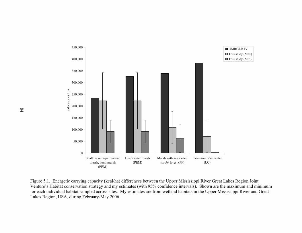
0
50,000
100,000
150,000
200,000
250,000
300,000
350,000
400,000
450,000
Shallow semi-permanentmarsh, hemi marsh
(PEM)
Deep-water marsh(PEM)
Marsh with associatedshrub/ forest (PF)
Extensive open water(LC)
Kilo
calo
ries /
ha
UMRGLR JVThis study (Max)This study (Min)
84
Figure 5.1. Energetic carrying capacity (kcal/ha) differences between the Upper Mississippi River Great Lakes Region Joint Venture’s Habitat conservation strategy and my estimates (with 95% confidence intervals). Shown are the maximum and minimum for each individual habitat sampled across sites. My estimates are from wetland habitats in the Upper Mississippi River and Great Lakes Region, USA, during February-May 2006. 84

85
UMRGLR Joint Venture waterfowl conservation strategy are designed to meet the
energetic demands of waterfowl populations that migrate and winter in the UMRGLR
(Soulliere 2007). Derivation of habitat goals is a function of the estimated waterfowl
population, energy density of habitat types (i.e., ECC), and the daily energy requirements
of ducks. I compared how much spring habitat would be required to support mallard,
lesser scaup, canvasback, blue-winged teal, northern pintail, and ring-necked duck
populations in the UMRGLR, using my estimates of ECC with those of the current
UMRGLR Joint Venture waterfowl habitat conservation strategy (Figure 5.2). According
to my results, spring habitat objectives for individual species such as mallards need to be
increased by only 5% to meet desired population objectives. However, spring habitat
objectives for scaup and canvasback need to be increased by 82% to meet desired
population objectives. My results suggest much more habitat is need for species that
heavily rely on deep water, lacustrine wetland habitat to meet energetic demands during
spring migration. For that reason, I recommend the UMRGLR JV adjust their habitat
objectives, especially for species other than mallards.
I encourage waterfowl managers and conservation planners in the UMRGLR Joint
Venture to reconsider assumed foraging values for habitats used by spring-migrating
waterfowl. Specifically, I suggest the UMRGLR Joint Venture adopt my estimates of
food energy abundance, as these estimates come from a sampling frame representing the
diversity of habitats that exist in the region. Priorities for conservation effort at the
national scale should recognize the importance preserving and enhancing habitats
encountered by waterfowl during spring migration. My results show that it is during this
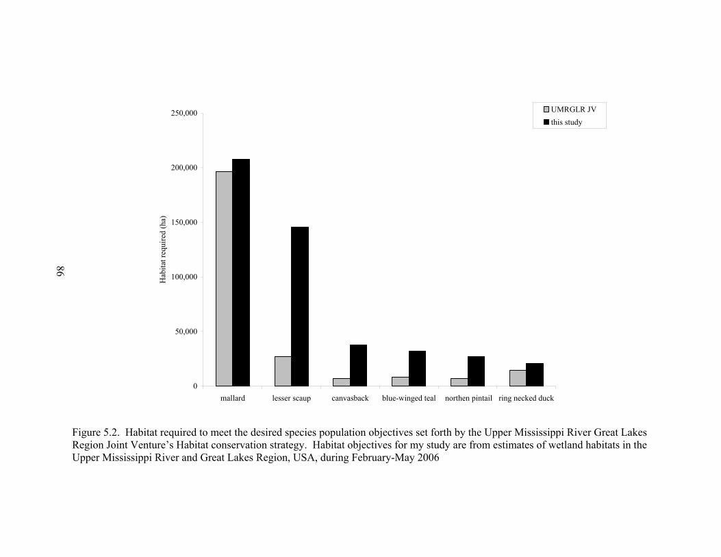
0
50,000
100,000
150,000
200,000
250,000
mallard lesser scaup canvasback blue-winged teal northen pintail ring necked duck
Hab
itat r
equi
red
(ha)
UMRGLR JVthis study
86
Figure 5.2. Habitat required to meet the desired species population objectives set forth by the Upper Mississippi River Great Lakes Region Joint Venture’s Habitat conservation strategy. Habitat objectives for my study are from estimates of wetland habitats in the Upper Mississippi River and Great Lakes Region, USA, during February-May 2006
86
87
time, that these habitats have the least capability to support energetic demands of
waterfowl. In addition, recent research has shown a strong link between the body
condition of female mallards arriving on the breeding grounds, and numerous
reproductive indicators (Devries et al. 2008). Without a doubt, factors such as food
abundance and availability have a direct and immediate effect on body condition.
Food energy abundance appears be more limiting during spring compared to
autumn migrations. Therefore, at a more local scale, wetland managers should consider
flooding wetlands in late winter or early spring, as this has shown to increase spring food
abundance (Greer et al. 2007). Though invertebrates did not contribute substantially to
total energy they likely still play a significant role in meeting other dietary requirements,
especially for female waterfowl. Hence, I suggest wetland managers ensure wetland
habitats provide both an abundance of invertebrates and seeds during the spring. Future
work should focus on the identifying the importance of invertebrates to spring migrating
waterfowl, especially for primarily carnivorous species, and investigate the possibility of
spring-migrating waterfowl being protein limited.
My study demonstrated differences among study sites in the UMRGLR in terms
of their ability to support migrating waterfowl. Conservation planners should identify
these areas where food density, energy, and habitat availability are comparatively low,
then determine the feasibility to restore, or enhance these habitats. For instance, the
Scioto River site had the least amount of overall habitat for spring migrating waterfowl,
although food density estimates were similar to other study sites. The overall lack of
habitat in the area likely reduced overall use of habitats even though they were capable of
supporting high densities of waterfowl. Further research is required to determine if

88
patterns that I observed hold true over multiple years. In addition, more reliable
estimates of “giving up” densities (i.e., foraging thresholds) as well as information
regarding the manner in which waterfowl will distribute themselves in relation to
available energy resources at multiple scales will further strengthen the biological
approach to conservation management in the UMRGLR.
89
LITERATURE CITED
Afton, A. D. 1984. Influence of age and time on reproductive performance of female Lesser Scaup. Auk 101:255–265.
Alerstam, T., and G. Högstedt. 1982. Bird migration and reproduction in relation to
habitats for survival and breeding. Ornis Scand 13:25–37. Alisauskas, R. T., and C. D. Ankney. 1992. The cost of egg laying and its relationship to
nutrient reserves in waterfowl. Pages 30–61 in B. D. J. Batt, A. D. Afton, M. G. Anderson, C. D. Ankney, D. H. Johnson, J. A. Kadlec, and G. L. Krapu, editors. Ecology and Management of Breeding Waterfowl. University of Minnesota Press, Minneapolis, Minnesota, USA.
Anderson, M. G., and J. B. Low. 1976. Use of sago pondweed by waterfowl on the
Delta Marsh, Manitoba. Journal of Wildlife Management 40:233–242. Anderson, J. T., and L. M. Smith. 1998. Protein and energy production in playas:
implications for migratory bird management. Wetlands 18:437-446. Ankney, C. D., and C.D. MacInnes. 1978. Nutrient reserves and reproductive
performance of female lesser snow geese. Auk 95:459–471.
Ankney, C. D. 1991. The role of nutrient reserves in limiting waterfowl reproduction. Condor 93:1029–1032.
Anteau, M. J., and A. D. Afton. 2004. Nutrient reserves of lesser scaup during spring migration in the Mississippi Flyway: a test of the Spring Condition Hypothesis. Auk 121:917–929.
______, and A. D. Afton. 2008. Amphipod densities and indices of wetland quality
across the Upper-Midwest, USA. Wetlands 28:184–196. Arzel, C., J. Elmberg, and M. Guillemain. 2006. Ecology of spring-migrating Anatidae:
a review. Journal of Ornithology. 147:167–184.
90
______,. Elmberg, M. Guillemain, P. Legagneux, F. Bosca, M. Chambouleyron, M. Lepley, C. Pin, A. Arnaud, and V. Schricke. 2007. Average mass of seeds encountered by foraging dabbling ducks in Western Europe. Wildlife Biology 13:328–336.
Badzinski, S. S., and S. A. Petrie. 2006. Diets of lesser and greater scaup during autumn
and spring on the lower Great Lakes. Wildlife Society Bulletin 34:664–674. Baldassare, G. A. 1980. Residual seeds as potential spring waterfowl foods in small, man-made impoundments. Prairie Naturalist 12:1–8. ______ and E. G. Bolen. 2006. Waterfowl Ecology and Management. Second edition.
Krieger Publishing Company, Malabar, Florida, USA. Ballard, B. M., J. E. Thompson, M. J. Petrie, J. M. Checkett, and D. G. Hewitt. 2004.
Diet and nutrition of northern pintails wintering along the southern coast of Texas. Journal of Wildlife Management 68:371–382.
Baranowski, T. E. 2007. Shorebird migration, habitat use and availability in the Lake
Erie Marshes region. Thesis, The Ohio State University, Columbus, USA. Bartonek, J. C., and J. J. Hickey. 1969. Selective feeding by juvenile diving ducks in
summer. Auk 86:443–457. Batt, B. D. J., A. D. Afton, M. G. Anderson, C. D. Ankney, D. H. Johnson, J. A. Kadlec,
and G. L. Krapu, editors. 1992. Ecology and Management of Breeding Waterfowl. University of Minnesota Press, Minneapolis, Minnesota, USA.
Bellrose, F. C. 1968. Waterfowl migration corridors east of the Rocky Mountains in the
United States. Illinois Natural History Survey Biological Notes. No. 61. 24 pp. ______ 1977. Species distribution, habitats, and characteristics of breeding dabbling
ducks in North America. Pages 1–17 in T. A. Bookhout, editor. Waterfowl and Wetlands – An Integrated Review. Proceedings of the 39th Midwest Fish and Wildlife Conference, Madison, Wisconsin, USA.
Bishop, C. T. 1990. Historical variation of water levels in Lakes Erie and Michigan-
Huron. Journal of Great Lakes Research 16:406–425. Bookhout, T. A., K. D. Bednarik, and R. W. Kroll. 1989. The Great Lakes marshes.
Pages 131–156 in L. M. Smith, R. L. Pederson, and R. M. Kaminski, editors. Habitat Management for Migrating and Wintering Waterfowl in North America. Texas Tech University Press, Lubbock, Texas, USA.
91
Boyer, M. W., J. D. Stafford., A. P.Yetter, C. S. Hine, M. M. Horath, and S. P. Havera. Moist-soil plant seed production for waterfowl at Chautauqua National Wildlife Refuge, Illinois. The American Midland Naturalist 154:331–341.
Brasher, M. E., J. D. Steckel, and R. J. Gates. 2007. Energetic carrying capacity of
actively and passively managed wetlands for migrating ducks in Ohio. Journal of Wildlife Management 71:2532–2541.
Burnham, K. P., and D. R. Anderson. 1998. Model selection and inference: a practical
information-theoretic approach. Springer-Verlag, New York, New York, USA. California Health Interview Survey. 2002. CHIS 2001 Methodology Series: Report 5 –
Weighting and Variance Estimation. Los Angeles, CA: UCLA Center for Health Policy Research.
Checkett, J. M., R. D. Drobney, M. J. Petrie, and D. A. Graber. 2002. True
metabolizable energy of moist-soil seeds. Wildlife Society Bulletin 30:1113–1119.
Coluccy, J. M., T. Yerkes, R. Simpson, J. W. Simpson, L. Armstrong, J. Davis. 2008. Population dynamics of breeding mallards in the Great Lakes states. Journal of Wildlife Management 72:1181–1187.
Conroy, M. J., and D. R. Smith. 1994. Designing large-scale surveys of wildlife abundance and diversity using statistical sampling principles. Transactions of the North American Wildlife and Natural Resources Conference 59:159–169.
Cowardin, L. M., V. Carter, and E. T. LaRoe. 1979. Classification of Wetlands and
Deepwater Habitats of the United States. U.S. Department of the Interior, Fish and Wildlife Service. FWS/OBS – 79/31.
Craven, S. R., and R. A. Hunt. 1984. Fall food habits of Canada geese in Wisconsin.
Journal of Wildlife Management 48:169–173. Dahl, T. E. 2006. Status and trends of wetlands in the conterminous United States 1998
to 2004. U.S. Department of the Interior; Fish and Wildlife Service, Washington, D.C. 112 pp.
Davis, E. S. 2002. Female choice and the benefits of mate guarding by male mallards.
Animal Behaviour. 64 (4): 619-628. Davis, L. W. 1993. Weed Seeds of The Great Plains: A handbook for identification.
Lawrence, KS: University Press of Kansas. 145 p.
92
Davis T. J. 1994. The Ramsar Convention Manual. A guide to the Convention of Wetlands of International Importance especially as waterfowl habitat. Ramsar Convention Bureau, Gland, Switzerland.
DiBona, M. T. 2007. Seasonal food availability for wintering and migrating dabbling
ducks and its implications for management at the Hackensack Meadowlands of New Jersey. Thesis, University of Delaware, Newark, Delaware, USA.
Delorit, R. J. 1970. An Illustrated Taxonomy Manual of Weed Seeds. Agronomy
Publications, River Falls Wisconsin, USA. Demarest, D. W., R. M. Kaminski, L. A. Brennan, and C. R. Boyle. 1997. Body-mass,
survival, and pairing consequences of winter-diet restriction in wood ducks. Journal of Wildlife Management 61:822–832.
Demissie, M. T., W. Soong, R. Allgire, L. Keefer, and P. Makowski. 1990. Cache River
basin: hydrology, hydraulics, and sediment transport, Vol. 1: background, data collection, and analysis. Illinois State Water Survey Contract Report, Champaign, Illinois, USA.
DeRoia, D. A., and T. A. Bookhout. 1989. Spring feeding ecology of teal on the Lake
Erie marshes. Ohio Journal of Science 89:3 Devries, J.H, R.W.Brook, D.W. Howerter, and M.G. Anderson. 2008. Effects of spring
body condition and age on reproduction in mallards (Anas platyrhncos). The Auk. 125 (3): 618-628.
Dobson, A. J. 1990. An introduction to generalized linear models. Chapman and Hall,
London. Dorge, C. L., W. J. Mitsch,. And J. R. Wiemhoff. 1984. Cypress wetlands in southern
Illinois. Pages 393–404 in K. C. Ewel and H. T. Odum, editors. Cypress swamps. University of Florida Press, Gainesville, Florida, USA.
DuBowy, P. J. 1988. Waterfowl communities and seasonal environments: Temporal
variability in interspecific competition. Ecology 69:1439–1453. Ducks Unlimited. 2005a. Development of a potential wetland restoration layer for
research and planning in the Great Lakes. Final Report. Submitted to the U.S. Fish and Wildlife Service, Upper Mississippi Great Lakes Joint Venture, 1 Federal Drive, Fort Snelling, MN. 32p. <http://www.ducks.org/media/Conservation /GLARO/_documents/_library/_gis/GLPotentialWetland.pdf.> Accessed 16 August, 2008.
93
Ducks Unlimited. 2005b. Updating the National Wetland Inventory (NWI) for the southern lower peninsula of Michigan. Final report submitted to the U.S. Fish and Wildlife Service Great Lakes Coastal Program Office. Ducks Unlimited’s Great Lakes / Atlantic Regional Office, Ann Arbor, Michigan, USA 38pp. <http://ww w.ducks.org/media/Conservation/GLARO/_documents/_library/_gis/NWI_FinalReport.pdf>. Accessed 15 August 15 2008.
Dugger, B. D., M. L. Moore, R. S. Finger, and M. J. Petrie. 2007. True metabolizeable
energy for seeds of common moist-soil plant species. Journal of Wildlife Management 71:1964–1967.
Environmental Systems Research Institute. [ESRI]. 2001. ArcGIS Spatial Analyst
Software, Version 9.0. ESRI 380 New York St., Redlands, California, USA. Ernst, L. R. 1980. Variance of the estimated mean for several imputation procedures.
Proceedings Survey Research: Methods Section. American Statistics. Association., pp. 716–720.
Euliss, N. H., Jr., and G. Grodhaus. 1987. Management of midges and other
invertebrates for waterfowl wintering in California. California Fish and Game 73:238–243.
Euliss, N. H., Jr., R. L. Jarvis, and D. S. Gilmer. 1991. Feeding ecology of waterfowl
wintering on evaporation ponds in California. Condor 93:582–590. Farney, R. A. 1975. Fall foods of ducks in Lake Erie marshes during high water years.
Thesis, The Ohio State University, Columbus, Ohio, USA. Flather, C. H., and J. R. Sauer. 1996, Using landscape ecology to test hypotheses about
large-scale abundance patterns in migratory birds. Ecology 77:28–35. Frayer, W. E., T. J. Monahan, D. C. Bowden, and F. A. Graybill. 1983. Status and
trends of wetlands and deepwater habitats of the conterminous United States, 1950’s to 1970’s. U.S. Fish and Wildlife Service, Washington, D.C. 33pp.
Frederick, R. B., E. E. Klass, G. A. Baldassarre, and K. J. Reinecke. 1984. A method for
sampling waste corn. Journal of Wildlife Management 48:298–303.
Fredrickson, L. H., and R. D. Drobney. 1979. Habitat utilization by post-breeding waterfowl. Pages 119–131 in T. A. Bookhout, editor. Waterfowl and Wetlands – An Integrated Review. Proceedings of the 39th Midwest Fish and Wildlife Conference, Madison, Wisconsin, USA.
94
_______and T. S. Taylor. 1982. Management of seasonally flooded impoundments for wildlife. Resource Publication 148. U.S. Dept. of Interior, Fish and Wildlife Service, Washington, D.C.
Fretwell, S. D. 1972. Populations in a seasonal environment. Princeton University
Press. Gammonley, J. H., and M. E. Heitmeyer. 1990. Behavior, body condition, and foods of
buffleheads and lesser scaups during spring migration through the Klamath Basin, California. Wilson Bulletin 102:672–683.
Gershunskaya, J., and L. Huff. 2004. Outlier Detection and Treatment in the Current
Employment Statistics Survey. Proceedings of the Section on Survey Research Methods, American Statistical Association.
Galatowitsch, S. M., and A. G. van der Valk, 1996. The vegetation of restored and
natural prairie wetlands. Ecological Applications 61:102–112. Grabaskas, M. E. 1993. Aquatic vegetation and migratory waterfowl use of closed (non-
hunted) and open (hunted) areas of Pools 4 and 5 of the Upper Mississippi River National Wildlife and Fish Refuge. Thesis, The Ohio State University, Columbus, Ohio, USA.
Greer A. K., B. D. Dugger, D. A. Graber, and M. J. Petrie. 2007. The effects of seasonal
flooding on seed availability for spring migrating waterfowl. Journal of Wildlife Management 71:1561–1566.
Gruenhagen, N. M., and L. H. Fredrickson. 1990. Food use by migratory female
Mallards in northwest Missouri. Journal of Wildlife Management 54:622–626. Haig, S. M. 1998. Molecular contributions to conservation. Ecology 79:413–425. Harper, D.G. 1982. Competitive foraging in mallards: ‘ideal free’ ducks. Animal
Behavior. 30: 575-584. Haukos, D. A., and L. M. Smith. 1993. Moist-soil management of playa lakes for migrating and wintering ducks. Wildlife Society Bulletin 21:288-298.
Havera, S. P. 1999. Waterfowl of Illinois: status and management. Illinois Natural
Survey Special Publication 21. xliii+ 628 pp. Heinrich, J. W., and S. R. Craven. 1992. The economic impact of Canada geese at the
Horicon Marsh, Wisconsin. Wildlife Society Bulletin 20:364–371.
95
Heitmeyer, M. E. 1985. Wintering strategies of female mallards related to dynamics of lowland hardwood wetlands in the upper Mississippi Delta. Dissertation, University of Missouri, Columbia, Missouri, USA.
______ 1988. Body composition of female mallards in winter in relation to annual cycle
events. Condor 90:669–680. ______ 1989. Agricultural/wildlife enhancement in California: The Central Valley
Habitat Joint Venture. Transactions of the North American Wildlife and Natural Resources Conference 54:391–402.
_______ 2006. The importance of winter floods to mallards in the Mississippi Alluvial
Valley. Journal of Wildlife Management 70:101–110. Hepp, G. R. 1984. Dominance in wintering Anatinae: potential effects on clutch size and
time of nesting. Wildfowl 35:132–134. Hidiroglou, M., and K. P. Srinath. 1981. Some estimators of a population total from
simple random samples containing large units. Journal of American statistics Association 76:690–695.
Hoekman, S. T., L. S. Mills, D. H. Howerter, J. H. Devries, and I. J. Ball. 2002.
Sensitivity analyses of the life cycle of mid-continent mallards. Journal of Wildlife Management 66:883–900.
Hoffman, R. D., and T. A. Bookhout. 1985. Metabolizable energy of seeds consumed by
ducks in Lake Erie marshes. Transactions of the North American Wildlife and Natural Resources Conference 50:557–565.
Hohman, W. L., T. S. Taylor, and M. W. Weller. 1988. Annual body weight change in
ring-necked ducks (Aythya collaris). Pages 257–269 in M. W. Weller, editor. Waterfowl in Winter. University Minnesota Press, Minneapolis, Minnesota, USA.
Hooge P. N., and B. Eichenlaub. 1997. Animal movement extension to Arcview,
version 1.1. U.S. Geological Survey, Anchorage, Alaska, USA. Hutchison, M. D., 1987. The Lower Cache River basin of southern Illinois. Erigenia 9:1–
54. Illinois State Water Survey [ISWS]. 2008. ISWS home page. <http:www.sws.uiuc.edu>. Accessed 15 August 2008. Jeffries, M. 2006. Invertebrate communities and turnover in wetland ponds affected by
drought. Freshwater Biology. 32(3): 603-612.

96
Johnson, A. M. 2007. Food abundance and energetic carrying capacity for wintering waterfowl in the Great Salt Lake wetlands. Thesis, Oregon State University, Corvallis, Oregon, USA.
Johnson, W. C., B. V. Millett, T. Gilmanvov, R. A Voldseth, B. R. Guntenspergen, and D. E. Naugle. 2005. Vulenerability of northern prairie wetlands to climate change. BioScience 55:863–872.
Johnston, C. A. 1984. Mapping Wisconsin’s wetlands. Wisconsin Natural Resources, 8 4–6.
Jorde, D. G., and R. B. Owen, Jr. 1988. Efficiency of nutrient use by American black ducks wintering in Maine. Journal of Wildlife Management 52:209–214.
______., M. Haramis, C. M. Bunck, and G. W. Pendleton. 1995. Effects of diet on rate of body mass gain by wintering canvasbacks. Journal of Wildlife Management 59:31–39.
Kaminski, R. M., J. B. Davis, H. W. Essig, P. D. Gerard, and K. J. Reinecke. 2003. True metabolizable energy for wood ducks from acorns compared to other waterfowl foods. Journal of Wildlife Management 67:542–550.
King, J. R. 1974. Seasonal allocation of time and resources in birds. Pages 4-85 in R. A.
Paynter, editor. Avian energetics. Nuttall Ornithological Club 15, Cambridge, Mas- sachusetts, USA.
Korschgen, C. E., L. S George, and W. L. Green. 1988. Feeding ecology of canvasbacks
staging on Pool 7 of the Upper Mississippi River. Pages 237–249 in M.W. Weller, editor. Waterfowl in Winter. University of Minnesota Press, Minneapolis, Minnesota, USA.
Koel, T. M., and R. E. Sparks. 2002. Historical patterns of river stage and fish
communities as criteria for operations of dams on the Illinois River. River Research and Applications 18:2–19.
Krapu, G. L., and G. A. Swanson. 1975. Some nutritional aspects of reproduction in
prairie nesting pintails. Journal of Wildlife Management 39:156–162. ______ 1981. The role of nutrient reserves in mallard reproduction. Auk 98:29–38. ______ and K. J. Reinecke. 1992. Foraging ecology and nutrition. Pages 1–29 in B. D.
J. Batt, A. D. Afton, M. G. Anderson, C. D. Ankney, D. H. Johnson, J. A. Kadlec, and G. L. Krapu, editors. Ecology and Management of Breeding Waterfowl. University of Minnesota Press, Minneapolis, Minnesota, USA.

97
Kross, J., R. M. Kaminski, K. J. Reinecke, E. J. Penny, A. T. Pearse. 2008. Moist-soil
seed abundance in managed wetlands in the Mississippi Alluvial Valley. Journal of Wildlife Management 72:707–714.
LaGrange, T. G. 1985. Habitat use and nutrient reserves dynamics of spring migratory mallards in central Iowa. Thesis, Iowa State University, Ames, Iowa, USA. ______ and J. J. Dinsmore. 1989. Habitat use by mallards during spring migration
through central Iowa. Journal of Wildlife Management 53:1076–1081. Lesaffre E, D. Rizopoulos, and R. Tsonaka. 2006. The logistic-transformation for
bounded outcome scores. Biostatistics 2006. Lovvorn, J. R. 1987. Behavior, energetics, and habitat relations of canvasback ducks
during winter and early spring migration. Dissertation, University of Wisconsin, Madison, Wisconsin, USA.
MacArthur, R. H. and Wilson, E. O. 1967. The Theory of Island Biogeography.
Princeton University Press. Princeton, New Jersey. Martin, A. C., and F. M. Uhler. 1951. Food of game ducks in the United States and
Canada. U.S. Fish and Wildlife Service Research Report 30. 308 pp. ______ and W. D. Barkley. 1961. Seed identification manual. University of California
Press, Berkeley, California, USA. Manley, S. W., R. M. Kaminski, K. J. Reinecke, and P. D. Gerard. 2004. Waterbird
foods in winter-managed ricefields in Mississippi. Journal of Wildlife Management 68:74–83.
McKinney, F., S.R. Derrickson, and P. Mineau. 1983. Forced Copulation in Waterfowl. Behavior. 86: 250-293. Midwestern Regional Climate Center [MRCC]. 2008. MRCC home page. <http://mcc.
sws.uiuc.edu/climate_midwest>. Accessed 15 August 2008.
Miller, M. R. 1986. Northern Pintail body condition during wet and dry winters in the Sacramento Valley, California. Journal of Wildlife Management 50:189–198.
______ and J. Eadie. 2006. The allometric relationship between resting metabolic rate
and body mass in wild waterfowl (Anatidae) and an application to estimation of winter habitat requirements. Condor 108:166–177.
98
Montgomery, F. H. 1977. Seeds and fruits of plants of eastern Canada and northeastern United States. University of Toronto Press, Toronto, Canada.
Murkin, H. R., and J. A. Kadlec. 1986. Relationships between waterfowl and
macroinvertebrate densities in a northern prairie marsh. Journal of Wildlife Management 50:212–217.
Nalepa, T. F., A. J. Wojcik, D. L., Fanslow, and G. A. Lang. 1995. Initial Colonization
of the zebra mussel (Dreissena polymorpha) in Saginaw Bay, Lake Huron: population recruitment, density and size structure. Journal of Great Lakes Research 1:417–434.
National Wetlands Inventory (NWI). 1990. Photointrepretation conventions for the
National Wetlands Inventory. U.S. Fish and Wildlife Service. National Wetlands Inventory Center, St. Petersburg, Florida, USA.
Naylor, L. W. 2002. Evaluating moist-soil seed production and management in Central
Valley wetlands to determine habitat needs for waterfowl. Thesis, University of California, Davis, California, USA.
Nelms, C. O., and D. J. Twedt. 1996. Seed deterioration in flooded agricultural fields
during winter. Wildlife Society Bulletin 24:85–88. Newton, I. 2006. Can conditions experienced during migration limit the populations
levels of birds? Journal of Ornithology. 147: 146-166. Nudds, T. D. 1983. Niche dynamics and organization of waterfowl guilds in variable
environments. Ecology 64:319–330. Olson, T. M. 2003. Variation in use of managed wetlands by waterfowl, wading birds,
and shorebirds in Ohio. Thesis, The Ohio State University, Columbus, Ohio, USA.
O’neal, B. J., E. J. Heske, and J. D. Stafford. 2008. Waterbird response to wetlands
restored through the Conservation Reserve Enhancement Program. Journal of Wildlife Management 72:654–664.
Pederson, G. B., and R. L. Pederson. 1983. Feeding ecology of mallards and pintails in
lower Klamath marshes. U.S. Fish and Wildlife Service final report. Humboldt State University Foundation, Arcata, California, USA. 89pp.
Pehrsson, O. 1984. Diving duck populations in relation to their food supplies. Pages
101–122 in P. R. Evans, J. D. Goss-Custard, and W. G. Hale, editors. Coastal Waders and Wildfowl in Winter. Cambridge University Press.
99
Petrie, M. J., R. D. Drobney, and D. A. Graber. 1998. True metabolizable energy estimates of Canada goose foods. Journal of Wildlife Management 62:1147–1152.
Poysa, H. 2001. Dynamics of habitat distribution in breeding mallards: assessing the
applicability of current habitat selection models. Oikos. 94: 365-373. Quinn G. P., and M. J. Keough. 2002. Experimental Design and Data Analysis for
Biologists. Cambridge University Press, Cambridge, New York, Melbourne, Madrid, Cape Town, 537 pp.
R Development Core Team (version 2.5.1). 2006. R: A Language and Environment for
Statistical Computing. R Foundation for Statistical Computing, Vienna, Austria. Reid, F. A., J. R. Kelley, T. S. Taylor, L. H. Fredrickson. 1989. Upper Mississippi
Valley Wetlands- Refuges and Moist-Soil Impoundments. Pages 181–202 in L. M. Smith, R. L. Pederson, and R. M. Kaminski, editors. Habitat Management for Migrating and Wintering Waterfowl in North America. Texas Tech University Press, Lubbock, Texas, USA.
Reinecke, K. J., R. M. Kaminski, D. J. Moorhead, J. D. Hodges, and J. R. Nassar, 1989.
Mississippi Alluvial Valley. Pages 203–247 in L. M. Smith, R. L. Pederson, and R. M. Kaminski, editors. Habitat Management for Migrating and Wintering Waterfowl in North America. Texas Tech University Press, Lubbock, Texas, USA.
______,and K. M. Hartke. 2005. Estimating moist-soil seeds available to waterfowl with
double sampling for stratification. Journal of Wildlife Management 69:794–799. Ricklefs, R. E. 1974. Energetics of reproduction in birds. Pages 152–292 in R. A
Paytner, Jr., editor. Avian Energetics. Nuttall Ornithological. Cambridge, Massachusetts, USA.
Riley, T. Z., and T. A. Bookhout. 1993. Response of dabbling ducks to early-spring
partial drawdown on Lake Erie marshes. Prairie Naturalist 25:13–18. SAS Institute. 1999. SAS/STAT User’s Guide. SAS Institute, Cary, North Carolina,
USA. Schloesser, D. W., and B. A. Manny. 1990. Decline of wild celery buds in the lower
Detroit River, 1950–85. Journal of Wildlife Management 54:72–76. Sherfy, M. H. 1999. Nutritional value and management of waterfowl and shorebird foods
in Atlantic Coastal moist-soil impoundments. Dissertation, Virginia Polytechnic Institute and State University, Blacksburg, Virginia, USA.
100
Smith, H. I. 1901. Summary of the archeology of Saginaw valley, Michigan. American
Anthropologist 3:286–293. Smith, R. V. 2007. Evaluation of waterfowl habitat and spring food selection by mallard
and lesser scaup on the Swan Lake Illinois Habitat Rehabilitation and Enhancement Project. Thesis, Southern Illinois University, Carbondale, Illinois, USA.
Soulliere, G. J., B. A. Potter, J. M. Coluccy, R. C. Gatti., C. L. Roy, D. R. Luukkonen, P.
W. Brown, and M. W. Eichholz. 2007. Upper Mississippi River and Great Lakes Region Joint Venture Waterfowl Habitat Conservation Strategy. U.S. Fish and Wildlife Service, Fort Snelling, Minnesota, USA.
Sparks, R. E., J. C. Nelson, and Y.Yin. 1998. Naturalization of the flood regime in
regulated rivers. BioScience 48:706–720. Stafford, J. D., R. M. Kaminski, K. J. Reinecke, and S. W. Manley. 2006a. Waste rice
for waterfowl in the Mississippi Alluvial Valley. Journal of Wildlife Management 70:61–69.
______, K. J. Reinecke, R. M. Kaminski, and P. D. Gerard. 2006b. Multi-stage
sampling for large scale natural resource surveys: a case study of rice and waterfowl. Journal of Environmental Management 78:353–361.
______, M. M. Horath, A. P.Yetter, C. S. Hine, and S. P. Havera. 2007. Wetland use by
mallards during spring and fall in the Illinois and central Mississippi River Valleys. Waterbirds 30:394–402.
Steckel, J. D. 2003. Food availability and waterfowl use on mid-migration habitats in
central and northern Ohio. Thesis, The Ohio State University, Columbus, Ohio, USA.
Stollberg, B. P. 1950. Food habits of shoal-water ducks on Horicon Marsh, Wisconsin.
Journal of Wildlife Management 14:214–217. Sugden, L. G. 1971. Metabolizable energy of small grains for mallards. Journal of
Wildlife Management 35:781–785. Swanson, G. A., G. L. Krapu, and J. R. Serie. 1979. Foods of laying female dabbling
ducks on the breeding grounds. Pages 59–70 in T. A. Bookhout, editor. Waterfowl and Wetlands – An Integrated Review, Proceedings of the 39th Midwest Fish and Wildlife Conference, Madison, Wisconsin, USA.
101
Taylor, T. S. 1978. Spring foods of migrating blue-winged teal on seasonally flooded impoundments. Journal of Wildlife Management 42:900–903.
The Nature Conservancy. 2008. Safeguarding the Scioto: Conservation Reserve
Enhancement Program. <http://www.nature.org/wherewework/northamerica /states/ohio/preserves/art14378.html>. accessed 17 August 2008.
Thompson, D. 1973. Feeding ecology of diving ducks on Keokuk pool, Mississippi
River. Journal of Wildlife Management 37:367–381.
Trauger, D. L., and J. H. Stoudt. 1978. Trends in waterfowl populations and habitats on study areas in Canadian parklands. Transactions of North American Wildlife and Natural Resources Conference 43:187–205.
Upper Mississippi River and Great Lakes Region [UMRGLR] Joint Venture
Management Board. 1998. Upper Mississippi River and Great Lakes Region Joint Venture Implementation Plan Update. U.S. Fish and Wildlife Service, Fort Snelling, Minnesota, USA.
U.S. Fish and Wildlife Service. 2004. Illinois River: National Wildlife and Fish Refuge
Complex Comprehensive Conservation Plan Approval. http://www.fws.gov/ midwest/planning/IllinoisRiver/index.html Accessed 15 August, 2008.
Van Eerden, M. R. 1984. Waterfowl movements in relation to food stocks. Pages 84–
100 in P. R. Evans, J. D. Goss-Custard, and W. G. Hale, editors. Coastal Waders and Wildfowl in Winter. Cambridge University Press.
Van Horn, K., K. Benton, and R. Gatti. 2006. Waterfowl breeding population survey for
Wisconsin, 1973–2006. Wisconsin Department of Natural Resources, Bureau of Wildlife Management, Madison Wisconsin.
Weller, M. W., editor. 1988. Waterfowl in winter. University Minnesota Press, Minneapolis, Minnesota, USA. Wersal, R. M., J. D. Madsen, B. R. McMillan, and P. D. Gerard. 2006. Environmental
factors affecting biomass and distribution of Stuckenia Pectinata in the Heron Lake System, Minnesota, USA. Wetlands 26:313–321.
Winslow, C. J. 2003. Estimation of waterfowl food abundance in coastal freshwater
marshes of Louisiana and Texas. Thesis, Louisiana State University, Baton Rouge, Louisiana, USA.
Wisconsin Department of Natural Resources. 2008. Wisconsin Waterfowl Strategic Plan
2008–2018. < http://prodwbin99.dnr.state.wi.us/org/land/wildlife/plan/plan2.pdf> Accessed 15 August 2008.
102
Wood, L. E. 1964. Bottom sediments of Saginaw Bay, Michigan. Journal of
Sedimentary Research 34:173–184. Wooten, D. E., and S. J. Werner. 2004. Food habits of lesser scaup aythya affinis
occupying baitfish aquaculture facilities in Arkansas. Journal of the World Aquaculture Society 35:70–77.
Whyte, R. J., and E. G. Bolen. 1984. Variation in winter fat depots and condition indices
of mallards. Journal of Wildlife Management 48:1370–1373. Yerkes T., K. A. Hobson, L. I. Wassenaar, R. Macleod, and J. M. Coluccy. 2008. Stable
isotopes (δD, δ13C, δ15N) reveal associations among geographic location and condition of Alaskan northern pintails. Journal of Wildlife Management 72:715–725.
Zimin V. B., A. V. Artemyev, and N. V. Lapshin. 2002. Survey of spring migrations
and stopovers in the Olonets fields in Karelia. Pages 18–28 in G.A. Noskov, A. Czajkowski, and K. P. Fertikova, editors. Study of the status and trends of migratory bird populations in Russia, Fourth issue. OMPO special publication, St Petersburg, Worlds and Family.

103
APPENDICES
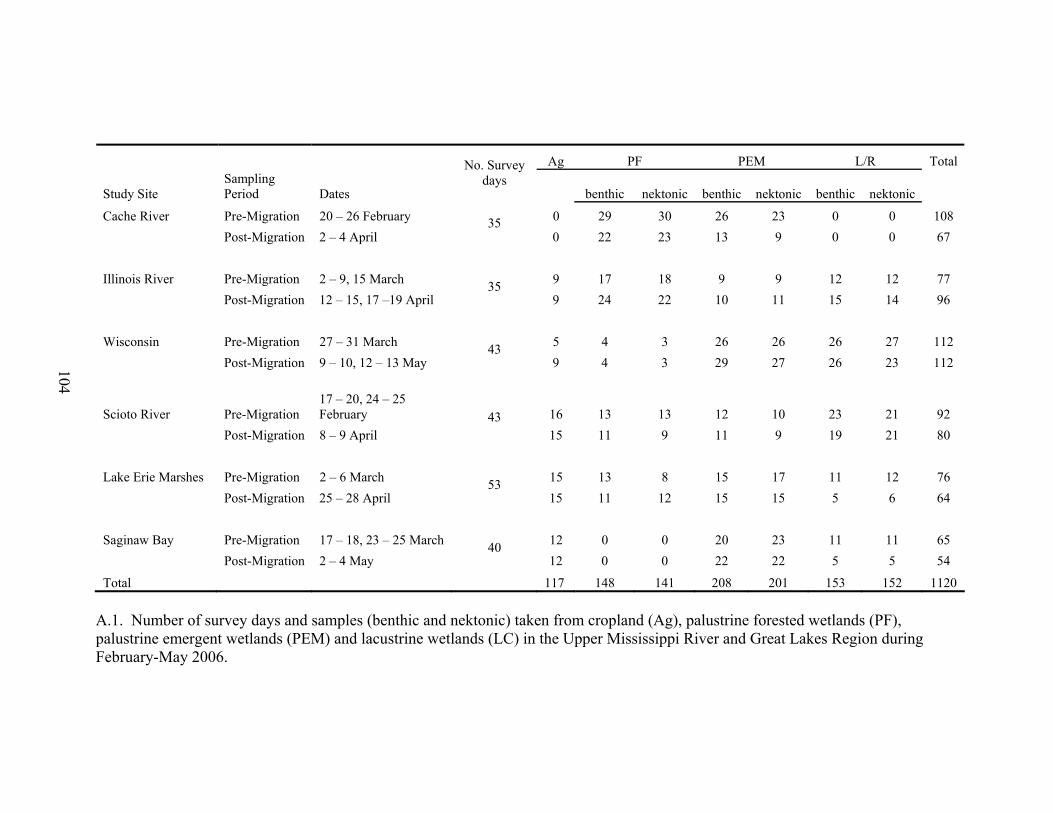
Ag PF PEM L/R Total No. Survey days
benthic nektonic benthic nektonic benthic nektonic Study Site Sampling Period Dates
Cache River Pre-Migration 20 – 26 February 0 29 30 26 23 0 0 108 35 0 22 23 13 9 0 0 Post-Migration 2 – 4 April 67
Illinois River Pre-Migration 2 – 9, 15 March 9 17 18 9 9 12 12 77 35
9 24 22 10 11 15 14 Post-Migration 12 – 15, 17 –19 April 96 Wisconsin Pre-Migration 27 – 31 March 5 4 3 26 26 26 27 112 43
9 4 3 29 27 26 23 Post-Migration 9 – 10, 12 – 13 May 112 104
Scioto River Pre-Migration 17 – 20, 24 – 25 February 16 13 13 12 10 23 21 92 43
15 11 9 11 9 19 21 Post-Migration 8 – 9 April 80 Lake Erie Marshes Pre-Migration 2 – 6 March 15 13 8 15 17 11 12 76 53
15 11 12 15 15 5 6 Post-Migration 25 – 28 April 64 Saginaw Bay Pre-Migration 17 – 18, 23 – 25 March 12 0 0 20 23 11 11 65 40
12 0 0 22 22 5 5 Post-Migration 2 – 4 May 54
Total 117 148 141 208 201 153 152 1120 A.1. Number of survey days and samples (benthic and nektonic) taken from cropland (Ag), palustrine forested wetlands (PF), palustrine emergent wetlands (PEM) and lacustrine wetlands (LC) in the Upper Mississippi River and Great Lakes Region during February-May 2006.
104
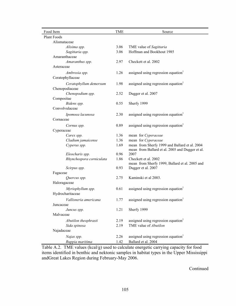
Food Item TME Source Plant Foods Alismataceae Alisima spp. 3.06 TME value of Sagittaria Sagittaria spp. 3.06 Hoffman and Bookhout 1985 Amaranthaceae Amaranthus spp. 2.97 Checkett et al. 2002 Asteraceae Ambrosia spp. 1.26 assigned using regression equation1 Ceratophyllaceae Ceratophyllum demersum 1.98 assigned using regression equation1 Chenopodiaceae Chenopodium spp. 2.52 Dugger et al. 2007 Compositae Bidens spp. 0.55 Sherfy 1999 Convolvulaceae Ipomoea lacunosa 2.30 assigned using regression equation1 Cornaceae Cornus spp. 0.89 assigned using regression equation1 Cyperaceae Carex spp. 1.36 mean for Cyperaceae Cladium jamaicense 1.36 mean for Cyperaceae Cyperus spp. 1.69 mean from Sherfy 1999 and Ballard et al. 2004
Eleocharis spp. 0.96 mean from Ballard et al. 2005 and Dugger et al. 2007
Rhynchospora corniculata 1.86 Checkett et al. 2002
Scirpus spp. 0.93 mean from Sherfy 1999, Ballard et al. 2005 and Dugger et al. 2007
Fagaceae Quercus spp. 2.75 Kaminski et al 2003. Haloragaceae Myriophyllum spp. 0.61 assigned using regression equation1 Hydrocharitaceae Vallisneria americana 1.77 assigned using regression equation1 Juncaceae Juncus spp. 1.21 Sherfy 1999 Malvaceae Abutilon theophrasti 2.19 assigned using regression equation1 Sida spinosa 2.19 TME value of Abutilon Najadaceae Najas spp. 2.26 assigned using regression equation1 Ruppia maritima 1.42 Ballard et al. 2004
Table A.2. TME values (kcal/g) used to calculate energetic carrying capacity for food items identified in benthic and nektonic samples in habitat types in the Upper Mississippi andGreat Lakes Region during February-May 2006.
Continued
105
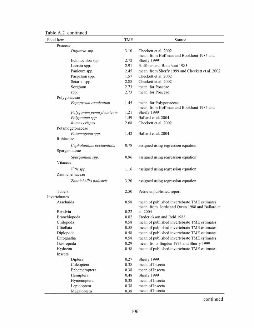
Table A.2 continued Food Item TME Source Poaceae Digitaria spp. 3.10 Checkett et al. 2002
Echinochloa spp. 2.72 mean from Hoffman and Bookhout 1985 and Sherfy 1999
Leersia spp. 2.91 Hoffman and Bookhout 1985 Panicum spp. 2.45 mean from Sherfy 1999 and Checkett et al. 2002 Paspalum spp. 1.57 Checkett et al. 2002 Setaria spp. 2.88 Checkett et al. 2002 Sorghum 2.73 mean for Poaceae spp. 2.73 mean for Poaceae Polygonaceae Fagopyrum esculentum 1.45 mean for Polygonaceae
Polygonum pennsylvanicum 1.21 mean from Hoffman and Bookhout 1985 and Sherfy 1999
Polygonum spp. 1.59 Ballard et al. 2004 Rumex crispus 2.68 Checkett et al. 2002 Potamogetonaceae Potamogeton spp. 1.42 Ballard et al. 2004 Rubiaceae Cephalanthus occidentalis 0.78 assigned using regression equation1 Sparganiaceae Sparganium spp. 0.96 assigned using regression equation1 Vitaceae Vitis spp. 1.16 assigned using regression equation1 Zannichelliaceae Zannichellia palustris 3.20 assigned using regression equation1 Tubers 2.50 Petrie unpublished report Invertebrates Arachnida 0.58 mean of published invertebrate TME estimates
Bivalvia 0.22 mean from Jorde and Owen 1988 and Ballard et al. 2004
Branchiopoda 0.82 Frederickson and Reid 1988 Chilopoda 0.58 mean of published invertebrate TME estimates Clitellata 0.58 mean of published invertebrate TME estimates Diplopoda 0.58 mean of published invertebrate TME estimates Entognatha 0.58 mean of published invertebrate TME estimates Gastropoda 0.29 mean from Sugden 1973 and Sherfy 1999 Hydozoa 0.58 mean of published invertebrate TME estimates Insecta Diptera 0.27 Sherfy 1999 Coleoptera 0.38 mean of Insecta Ephemeroptera 0.38 mean of Insecta Hemiptera 0.48 Sherfy 1999 Hymenoptera 0.38 mean of Insecta Lepidoptera 0.38 mean of Insecta Megaloptera 0.38 mean of Insecta
continued
106
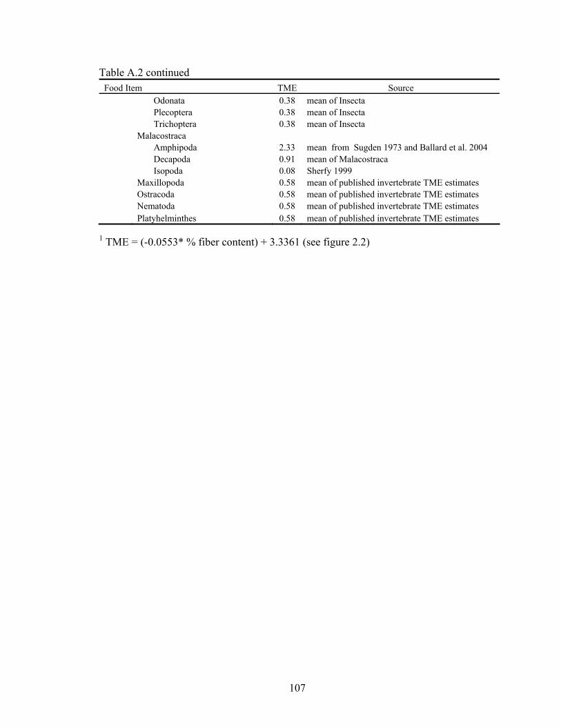
Table A.2 continued Food Item TME Source Odonata 0.38 mean of Insecta Plecoptera 0.38 mean of Insecta Trichoptera 0.38 mean of Insecta Malacostraca Amphipoda 2.33 mean from Sugden 1973 and Ballard et al. 2004 Decapoda 0.91 mean of Malacostraca Isopoda 0.08 Sherfy 1999 Maxillopoda 0.58 mean of published invertebrate TME estimates Ostracoda 0.58 mean of published invertebrate TME estimates Nematoda 0.58 mean of published invertebrate TME estimates Platyhelminthes 0.58 mean of published invertebrate TME estimates
1 TME = (-0.0553* % fiber content) + 3.3361 (see figure 2.2)
107
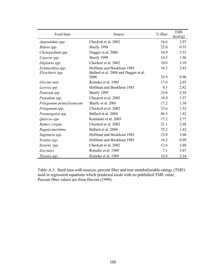
Food Item Source % fiber TME (kcal/g)
Amaranthus spp. Checkett et al. 2002 16.6 2.97Bidens spp. Sherfy 1999 22.0 0.55Chenopodium spp. Dugger et al. 2006 16.9 2.52Cyperus spp. Sherfy 1999 14.5 1.96Digitaria spp. Checkett et al. 2002 10.0 3.10Echinochloa spp. Hoffman and Bookhout 1985 18.2 2.82Eleocharis spp. Ballard et al. 2004 and Dugger et al.
2006 32.9 0.96Glycine max Reineke et al. 1989 17.6 2.65Leersia spp. Hoffman and Bookhout 1985 9.3 2.82Panicum spp. Sherfy 1999 25.0 2.54Paspalum spp. Checkett et al. 2002 18.9 1.57Polygonum pennsylvanicum Sherfy et al. 2001 17.2 1.30Polygonum spp. Checkett et al. 2002 23.6 1.52Potamogeton spp. Ballard et al. 2004 46.5 1.42Quercus spp. Kaminski et al. 2003 17.2 2.77Rumex crispus Checkett et al. 2002 21.1 2.68Ruppia maritima Ballard et al. 2004 35.2 1.42Sagittaria spp. Hoffman and Bookhout 1985 23.0 3.06Scirpus spp. Hoffman and Bookhout 1985 16.2 0.99Setaria spp. Checkett et al. 2002 12.6 2.88Zea mays Reineke et al. 1989 7.1 3.67Zizania spp. Reineke et al. 1989 10.4 3.34
Table A.3. Seed taxa with sources, percent fiber and true metabolizeable energy (TME) used in regression equations which predicted seeds with no published TME value. Percent fiber values are from Havera (1999).
108
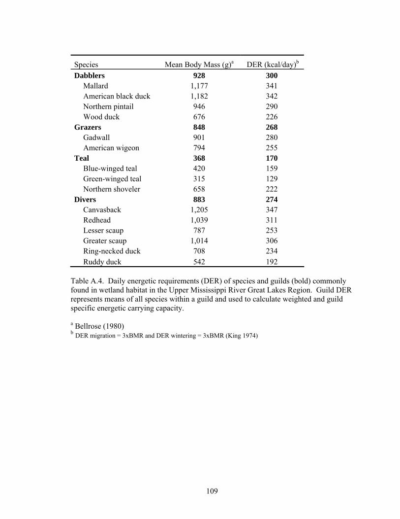
Species Mean Body Mass (g)a DER (kcal/day)b Dabblers 928 300 Mallard 1,177 341 American black duck 1,182 342 Northern pintail 946 290 Wood duck 676 226 Grazers 848 268 Gadwall 901 280 American wigeon 794 255 Teal 368 170 Blue-winged teal 420 159 Green-winged teal 315 129 Northern shoveler 658 222 Divers 883 274 Canvasback 1,205 347 Redhead 1,039 311 Lesser scaup 787 253 Greater scaup 1,014 306 Ring-necked duck 708 234 Ruddy duck 542 192
Table A.4. Daily energetic requirements (DER) of species and guilds (bold) commonly found in wetland habitat in the Upper Mississippi River Great Lakes Region. Guild DER represents means of all species within a guild and used to calculate weighted and guild specific energetic carrying capacity. a Bellrose (1980) b DER migration = 3xBMR and DER wintering = 3xBMR (King 1974)
109
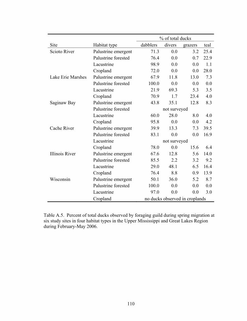
% of total ducks Site Habitat type dabblers divers grazers teal Scioto River Palustrine emergent 71.3 0.0 3.2 25.4 Palustrine forested 76.4 0.0 0.7 22.9 Lacustrine 98.9 0.0 0.0 1.1 Cropland 72.0 0.0 0.0 28.0Lake Erie Marshes Palustrine emergent 67.9 11.8 13.0 7.3 Palustrine forested 100.0 0.0 0.0 0.0 Lacustrine 21.9 69.3 5.3 3.5 Cropland 70.9 1.7 23.4 4.0Saginaw Bay Palustrine emergent 43.8 35.1 12.8 8.3 Palustrine forested not surveyed Lacustrine 60.0 28.0 8.0 4.0 Cropland 95.8 0.0 0.0 4.2Cache River Palustrine emergent 39.9 13.3 7.3 39.5 Palustrine forested 83.1 0.0 0.0 16.9 Lacustrine not surveyed Cropland 78.0 0.0 15.6 6.4Illinois River Palustrine emergent 67.6 12.8 5.6 14.0 Palustrine forested 85.5 2.2 3.2 9.2 Lacustrine 29.0 48.1 6.5 16.4 Cropland 76.4 8.8 0.9 13.9Wisconsin Palustrine emergent 50.1 36.0 5.2 8.7 Palustrine forested 100.0 0.0 0.0 0.0 Lacustrine 97.0 0.0 0.0 3.0 Cropland no ducks observed in croplands
Table A.5. Percent of total ducks observed by foraging guild during spring migration at six study sites in four habitat types in the Upper Mississippi and Great Lakes Region during February-May 2006.
110
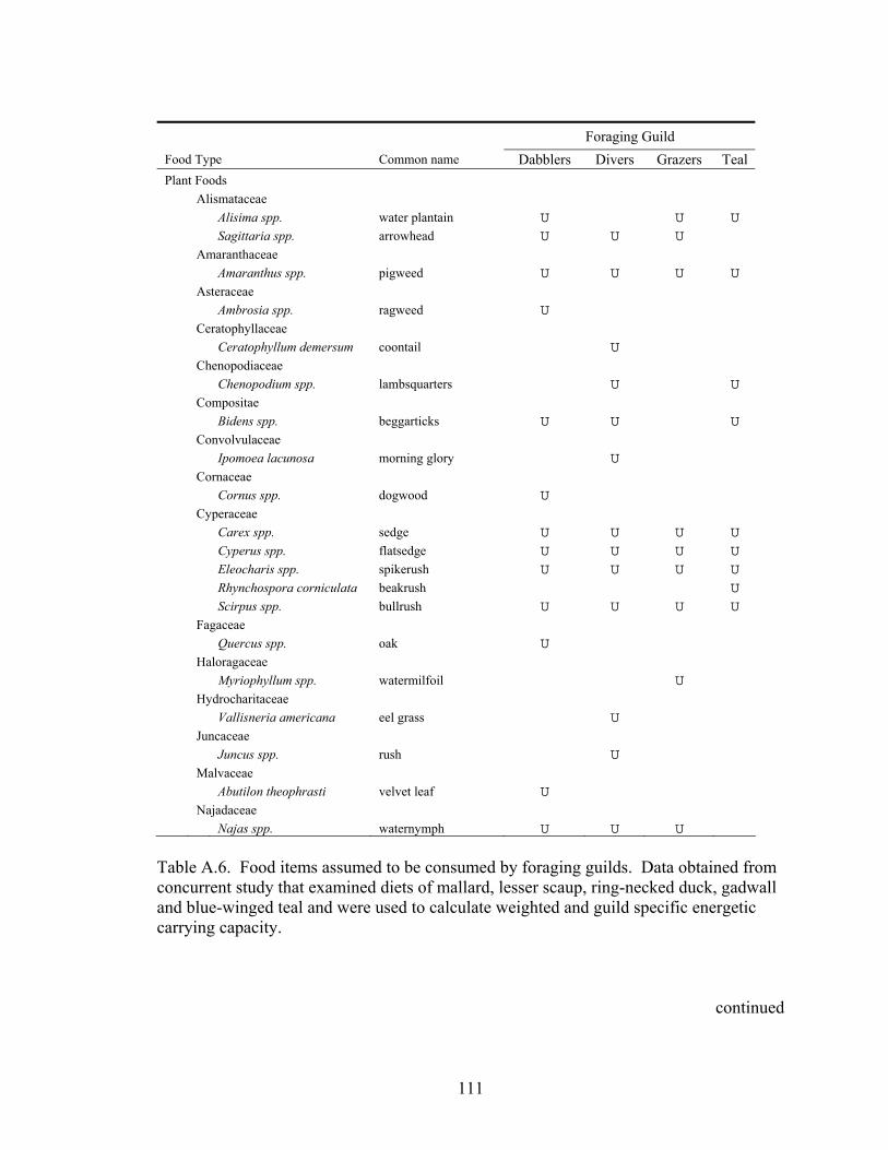
Foraging Guild Food Type Common name Dabblers Divers Grazers Teal Plant Foods Alismataceae Alisima spp. water plantain U U U Sagittaria spp. arrowhead U U U Amaranthaceae Amaranthus spp. pigweed U U U U Asteraceae Ambrosia spp. ragweed U Ceratophyllaceae Ceratophyllum demersum coontail U Chenopodiaceae Chenopodium spp. lambsquarters U U Compositae Bidens spp. beggarticks U U U Convolvulaceae Ipomoea lacunosa morning glory U Cornaceae Cornus spp. dogwood U Cyperaceae Carex spp. sedge U U U U Cyperus spp. flatsedge U U U U Eleocharis spp. spikerush U U U U Rhynchospora corniculata beakrush U Scirpus spp. bullrush U U U U Fagaceae Quercus spp. oak U Haloragaceae Myriophyllum spp. watermilfoil U Hydrocharitaceae Vallisneria americana eel grass U Juncaceae Juncus spp. rush U Malvaceae Abutilon theophrasti velvet leaf U Najadaceae Najas spp. waternymph U U U
Table A.6. Food items assumed to be consumed by foraging guilds. Data obtained from concurrent study that examined diets of mallard, lesser scaup, ring-necked duck, gadwall and blue-winged teal and were used to calculate weighted and guild specific energetic carrying capacity.
continued
111

Table A.6 continued
Foraging Guild Food Type Common name Dabblers Divers Grazers Teal Poaceae Digitaria spp. crabgrass U U U Echinochloa spp. millet U U U U Leersia spp. rice cut-grass U U U U Panicum spp. panic grass U U U U Setaria spp. bristlegrass U spp. grasses U U Polygonaceae
Polygonum pennsylvanicum
pennsylvania smartweed U U U U
Polygonum spp. smartweed U U U U Rumex crispus dock U U Potamogetonaceae Potamogeton spp. pondweed U U U U Rubiaceae Cephalanthus occidentalis buttonbush U U U U Sparganiaceae Sparganium spp. bur-reed U Vitaceae Vitis spp. grape U Zannichelliaceae Zannichellia palustris horned pondweed U Tubers U U Invertebrates Bivalvia mollusks, clams U U Branchiopoda fairy shrimp U U U Chilopoda centipedes U Clitellata earthworms, leaches U U U U
Entognatha ametabolous arthropods U U
Gastropoda snails U U U U Insecta Diptera flies U U U U Coleoptera beetles U U Ephemeroptera mayflies U Hemiptera aphids U U Hymenoptera bees, wasps, ants Lepidoptera butterflies U U
Odonata dragon flies, damselflies U U U
Trichoptera cadisflies U U continued
112

Table A.6 continued
Foraging Guild Food Type Common name Dabblers Divers Grazers Teal Malacostraca Amphipoda fresh water shrimp U U U U Isopoda sowbugs U U U U Maxillopoda copepods U U U Ostracoda seed shrimp U U U Nematoda roundworms U U U Gastropoda U U U U
113
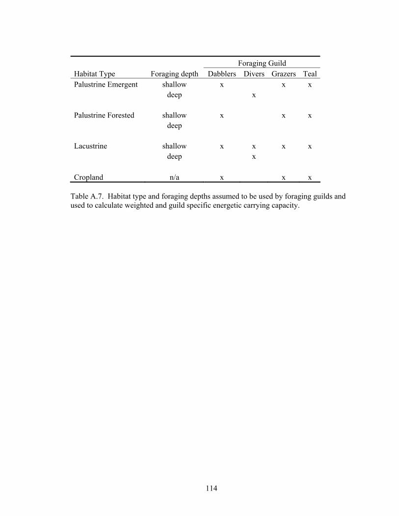
Foraging Guild Habitat Type Foraging depth Dabblers Divers Grazers Teal Palustrine Emergent shallow x x x deep x Palustrine Forested shallow x x x deep Lacustrine shallow x x x x deep x Cropland n/a x x x
Table A.7. Habitat type and foraging depths assumed to be used by foraging guilds and used to calculate weighted and guild specific energetic carrying capacity.
114
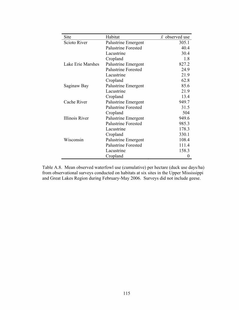
Site Habitat x⎯ observed use Scioto River Palustrine Emergent 305.1 Palustrine Forested 40.4 Lacustrine 30.4 Cropland 1.8 Lake Erie Marshes Palustrine Emergent 827.2 Palustrine Forested 24.9 Lacustrine 21.9 Cropland 62.8 Saginaw Bay Palustrine Emergent 85.6 Lacustrine 21.9 Cropland 13.4 Cache River Palustrine Emergent 949.7 Palustrine Forested 31.5 Cropland 504 Illinois River Palustrine Emergent 949.6 Palustrine Forested 985.3 Lacustrine 178.3 Cropland 330.1 Wisconsin Palustrine Emergent 108.4 Palustrine Forested 111.4 Lacustrine 158.3 Cropland 0
Table A.8. Mean observed waterfowl use (cumulative) per hectare (duck use days/ha) from observational surveys conducted on habitats at six sites in the Upper Mississippi and Great Lakes Region during February-May 2006. Surveys did not include geese.
115

116
Foraging guild (ECCguild)
Site Habitat dabblers divers grazers teal SR Palustrine Emergent 882 450 538 1461
Palustrine Forested 367 n/a 328 619 Lacustrine 58 269 40 101 Cropland 121 n/a 135 213
LE Palustrine Emergent 387 63 671 1121 Palustrine Forested 578 n/a 75 131 Lacustrine 75 156 41 60 Cropland 155 n/a 173 273
SB Palustrine Emergent 455 30 546 847 Lacustrine 19 22 13 22 Cropland 1472 n/a 1647 2597
CA Palustrine Emergent 323 661 403 673 Palustrine Forested 612 n/a 86 168
IR Palustrine Emergent 712 82 433 689 Palustrine Forested 976 n/a 250 398 Lacustrine 93 331 148 238 Cropland 2724 n/a 3049 4807
WI Palustrine Emergent 1274 41 930 1451 Palustrine Forested 644 n/a 318 569 Lacustrine 87 503 54 84 Cropland 1318 n/a 1476 2327
Table A.9. Duck use day/ha estimates of specific foraging guilds (ECCguild) in habitats sampled in the Upper Mississippi and Great Lakes Region during February-May 2006. Estimates were calculated using multistage sampling and using guild specific daily energy, diet, and habitat requirements.