Energetic boundary element method for accurate solution of

J Eng Math (2021) 127:29https://doi.org/10.1007/s10665-021-10100-y

Energetic boundary element method for accurate solution ofdamped waves hard scattering problems

Alessandra Aimi · Mauro Diligenti ·Chiara Guardasoni

Received: 6 October 2020 / Accepted: 31 January 2021 / Published online: 26 March 2021© The Author(s) 2021

Abstract The paper deals with the numerical solution of 2D wave propagation exterior problems including viscousand material damping coefficients and equipped by Neumann boundary condition, hence modeling the hard scatter-ing of damped waves. The differential problem, which includes, besides diffusion, advection and reaction terms, iswritten as a space–time boundary integral equation (BIE) whose kernel is given by the hypersingular fundamentalsolution of the 2D damped waves operator. The resulting BIE is solved by a modified Energetic Boundary ElementMethod, where a suitable kernel treatment is introduced for the evaluation of the discretization linear system matrixentries represented by space–time quadruple integrals with hypersingular kernel in space variables. A wide varietyof numerical results, obtained varying both damping coefficients and discretization parameters, is presented andshows accuracy and stability of the proposed technique, confirming what was theoretically proved for the simplerundamped case. Post-processing phase is also taken into account, giving the approximate solution of the exteriordifferential problem involving damped waves propagation around disconnected obstacles and bounded domains.

Keywords Damped wave equation · Energetic boundary element method · Hard scattering · Hypersingular kernel ·Weak boundary integral formulation

Mathematics Subject Classification 65M38

1 Introduction

Wave propagation problems are widely studied because they model a variety of phenomena in everyday life. Inthis context, while elastic forces tend to maintain the oscillatory motion, the transient effect vanishes because of

Alessandra Aimi, Mauro Diligenti and Chiara Guardasoni—Members of INdAM-GNCS Research Group.

A. Aimi · M. Diligenti · C. Guardasoni (B)Department of Mathematical, Physical and Computer Sciences, University of Parma, Parco Area delle Scienze, 53/A, 43126Parma, Italy e-mail: [email protected]

A. Aimie-mail: [email protected]

M. Diligentie-mail: [email protected]

123

http://crossmark.crossref.org/dialog/?doi=10.1007/s10665-021-10100-y&domain=pdf

https://orcid.org/0000-0002-4699-4261

http://orcid.org/0000-0002-7054-8579

29 Page 2 of 30 A. Aimi et al.

energy dissipation process, referred to as damping. Usually, the dissipation is generated by the interaction betweenthe waves and the propagation medium. On the other side, for instance in mechanical systems, since damping hasthe effect of reducing the amplitude of vibrations, it is desirable to have some amount of damping in order to fasterachieve an equilibrium configuration. Hence, damping is whether an unavoidable presence in physical reality or adesired characteristic in industrial design (see e.g., the applicative papers [1–4]).

For these reasons, it is interesting to consider damping terms into the modeling partial differential equations(PDEs): well-known examples are, for instance, the Klein–Gordon or the Telegraph equations (see e.g. [5] andreferences therein). For what concerns their approximate resolution, while the application of advanced numericaltechniques, such as finite element (FEM) and finite difference (FDM) methods, is well established, the Boundaryelement method (BEM) analysis of dissipation through damped wave equation rewritten as a boundary integralequation (BIE) is a relatively recent research topic [6–8] and not yet sufficiently investigated. Note that BEMsare ideally suited for solving problems defined in unbounded domains, such as wave propagation scattering byfinite obstacles, because they (i) rewrite the problem over the bounded obstacle and (ii) implicitly fulfill prescribedsolution behavior at infinity. Let us further remark that for the numerical solution of this kind of problems, oneneeds consistent approximations and accurate simulations even on large time domains of analysis.

In principle, both frequency domain [9,10] and time domain [11,12] BEM can be used for hyperbolic initial-boundary value problems. Space–time BEM has the advantage that it directly gives the unknown time-dependentquantities; in the case of unbounded domain problems, this is very beneficial. Let us note that Dirichlet absorbingboundary condition methods (see [13–17]) share the same feature. For space–time BEM, the construction of theBIEs, via boundary integral representation formula of the PDE solution, uses the fundamental solution of thehyperbolic differential operator at hand, if available, and jump relations [18]. The mathematical background oftime-dependent BIEs is summarized by Costabel in [19].

This paper deals with the numerical solution of wave propagation problems exterior to open arcs in the plane,including viscous and material damping coefficients into the PDE, and equipped by Neumann boundary conditionand homogeneous initial conditions. The numerical study of damped waves hard scattering model is a challengingtask due to the presence of advection and reaction terms, and the adopted methodology generalizes what hasbeen done in [20] for the much simpler undamped case. The differential problem is written as a space–time BIEwhose kernel is given by the hypersingular fundamental solution of the 2D damped waves operator. The integralproblem is then solved by a modified energetic BEM, appeared for the first time in its original form in [21]. Here, asuitable kernel treatment is introduced for the efficient evaluation of the discretization linear system matrix entriesrepresented by space–time quadruple integrals with hypersingular kernel in space variables having no analyticaltime integration available, differently from the undamped case.

The paper is structured as follows: at first, we present the differential model problem on an unbounded 2D domainand its BIE energetic weak formulation. Section 3 briefly summarizes, for reader’s convenience, the main featuresof Energetic BEM discretization which leads to a final linear system having a lower triangular block Toeplitzmatrix. Section 4 highlights the new approach introduced for the evaluation of quadruple space–time integrals withhypersingular damped kernel, giving some details about the adopted quadrature schemes, while in Sect. 5, a widevariety of significant results are presented and discussed, showing, from a numerical point of view, stability andaccuracy of the proposed technique, theoretically proved for the undamped case in [20]. Post-processing phase isalso taken into account, giving the numerical solution of the exterior differential problem involving damped wavespropagation around disconnected obstacles and bounded domains. Conclusions and ongoing research are reportedin the last Section.

123

Energetic BEM for damped waves hard scattering problems Page 3 of 30 29

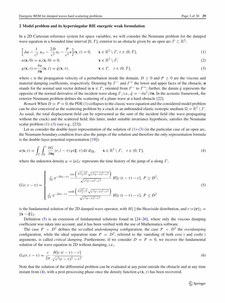
2 Model problem and its hypersingular BIE energetic weak formulation

In a 2D Cartesian reference system for space variables, we will consider the Neumann problem for the dampedwave equation in a bounded time interval [0, T ], exterior to an obstacle given by an open arc Γ ⊂ R

2:

[Δu − 1

c2 utt − 2D

c2 ut − P

c2 u](x, t) = 0, x ∈ R

2 \ Γ, t ∈ (0, T ], (1)

u(x, 0) = ut (x, 0) = 0, x ∈ R2 \ Γ, (2)

q(x, t):=∂u

∂n(x, t) = q̄(x, t), x ∈ Γ, t ∈ (0, T ], (3)

where c is the propagation velocity of a perturbation inside the domain, D ≥ 0 and P ≥ 0 are the viscous andmaterial damping coefficients, respectively. Denoting by Γ − and Γ + the lower and upper faces of the obstacle, nstands for the normal unit vector defined in x ∈ Γ , oriented from Γ − to Γ +; further, the datum q̄ represents theopposite of the normal derivative of the incident wave along Γ , i.e., q̄ = −∂uI /∂n. In the acoustic framework, theexterior Neumann problem defines the scattering of a plane wave at a hard obstacle [22].

RemarkWhen D = P = 0, the PDE (1) collapses to the classic wave equation and the considered model problemcan be also conceived as the scattering problem by a crack in an unbounded elastic isotropic medium � = R

2 \ Γ .As usual, the total displacement field can be represented as the sum of the incident field (the wave propagatingwithout the crack) and the scattered field; this latter, under suitable invariance hypothesis, satisfies the Neumannscalar problem (1)–(3) (see e.g., [23]).

Let us consider the double-layer representation of the solution of (1)–(3) (in the particular case of an open arc,the Neumann boundary condition fixes also the jumps of the solution and therefore the only representation formulais the double-layer potential representation [19]):

u(x, t) =∫

Γ

∫ t

0

∂G

∂nξ(r, t − τ) ϕ(ξ , τ ) dτ dγξ , x ∈ R

2 \ Γ, t ∈ (0, T ], (4)

where the unknown density ϕ = [u]Γ represents the time history of the jump of u along Γ ,

G(r, t − τ) =

⎧⎪⎪⎪⎪⎪⎪⎨⎪⎪⎪⎪⎪⎪⎩

c2π

e−D(t−τ)cos

(√P−D2c

√c2(t−τ)2−r2

)√

c2(t−τ)2−r2H [c (t − τ) − r ], P ≥ D2,

c2π

e−D(t−τ)cosh

(√D2−Pc

√c2(t−τ)2−r2

)√

c2(t−τ)2−r2H [c (t − τ) − r ], P ≤ D2

(5)

is the fundamental solution of the 2D damped wave operator, with H [·] the Heaviside distribution, and r :=‖r‖2 =‖x − ξ‖2.

Definition (5) is an extension of fundamental solutions found in [24–26], where only the viscous dampingcoefficient was taken into account, and it has been verified with the use of Mathematica software.

The case P > D2 defines the so-called underdamping configuration, the case P < D2 the overdampingconfiguration, while the ideal separation state P = D2, referred to the vanishing of both cos(·) and cosh(·)arguments, is called critical damping. Furthermore, if we consider D = P = 0, we recover the fundamentalsolution of the wave equation in 2D without damping, i.e.,

G0(r, t − τ) = c

2π

H [c (t − τ) − r ]√c2(t − τ)2 − r2

. (6)

Note that the solution of the differential problem can be evaluated at any point outside the obstacle and at any timeinstant from (4), with a post-processing phase once the density function ϕ(x, t) has been recovered.

123


To this aim, applying a directional (normal) derivative w.r.t. x in (4), performing a limiting process for x tendingto Γ and using the assigned Neumann boundary condition (3), we obtain the hypersingular space–time BIE∫

Γ

∫ t

0

∂2G

∂nx∂nξ

(r, t − τ)ϕ(ξ , τ ) dτ dγξ = q̄(x, t), x ∈ Γ, t ∈ [0, T ], (7)

in the unknown ϕ(x, t), which can be written with the compact notation

Dϕ = q̄. (8)

The equivalence of (8) with the initially given differential model problem (1)–(3) has been stated for generaltime-dependent problems in [19].

In order to properly manage equation (8), we introduce the following results.

Proposition 1 Defining the auxiliary kernel G̃(r, t − τ) as

⎧⎪⎪⎨⎪⎪⎩

√P−D2

2πe−D(t−τ) sin

(√P−D2

c

√c2(t − τ)2 − r2

)H [c (t − τ) − r ], P ≥ D2,

−√D2−P2π

e−D(t−τ) sinh(√

D2−Pc

√c2(t − τ)2 − r2

)H [c (t − τ) − r ], P ≤ D2,

(9)

representation formula (4) can be rewritten explicitly for x ∈ R2 \ Γ and t ∈ (0, T ] as

u(x, t) =∫

Γ

∫ t

0

r · nξ

r

{G(r, t − τ)

[ϕτ (ξ , τ ) + Dϕ(ξ , τ )

c+ ϕ(ξ , τ )

c(t − τ) + r

]+ G̃(r, t − τ)

ϕ(ξ , τ )

c(t − τ) + r

}

× dτ dγξ . (10)

Proof Let us consider the case P ≥ D2; starting from the definition of the double-layer potential in the right-handside of (4), we observe that

∂G

∂nξ

(r, t − τ) = ∂G

∂r(r, t − τ)

∂r

∂nξ

= c

2 πe−D(t−τ),

∂

∂r

[cos

(√P − D2

c

√c2(t − τ)2 − r2

) 1√c(t − τ) + r

H [c(t − τ) − r ]√c(t − τ) − r

] ∂r

∂nξ

= c

2 πe−D(t−τ)

[√P − D2

csin

(√P − D2

c

√c2(t − τ)2 − r2

) r H [c(t − τ) − r ]c2(t − τ)2 − r2

−1

2cos

(√P − D2

c

√c2(t − τ)2 − r2

) 1

c(t − τ) + r

H [c(t − τ) − r ]√c2(t − τ)2 − r2

+ cos(√

P − D2

c

√c2(t − τ)2 − r2

) 1

c√c(t − τ) + r

∂

∂τ

H [c(t − τ) − r ]√c(t − τ) − r

] ∂r

∂nξ

.

Now, considering the integration over Γ × (0, t) of the above expression multiplied by ϕ(ξ , τ ), integrating in thesense of distributions the term containing the derivative with respect to τ and then expressing explicitly

∂

∂τ

[e−D(t−τ) cos

(√P − D2

c

√c2(t − τ)2 − r2

) 1

c√c(t − τ) + r

],

one finally deduces the thesis. When P < D2 we can proceed in the same manner, remembering that cos(i ·) =cosh(·) and sin(i ·) = i sinh(·), being i the imaginary unit. �Proposition 2 The space–time hypersingular integral operator D admits the following explicit expression:

Dϕ(x, t) =∫

Γ

∫ t

0

{(nx · nξ

r− r · nx r · nξ

r3

)

123


×[G(r, t − τ)

(ϕτ (ξ , τ ) + Dϕ(ξ , τ )

c+ ϕ(ξ , τ )

c(t − τ) + r

)+ G̃(r, t − τ)

ϕ(ξ , τ )

c(t − τ) + r

]

−r · nx r · nξ

r2

[G(r, t − τ)

(1

c2 [ϕττ (ξ , τ ) + 2Dϕτ (ξ , τ ) + D2ϕ(ξ , τ )]

+2ϕτ (ξ , τ ) + Dϕ(ξ , τ )

c[c(t − τ) + r ] +(

3

[c(t − τ) + r ]2 − P − D2

c2

c(t − τ) − r

c(t − τ) + r

)ϕ(ξ , τ )

)

+G̃(r, t − τ)

(2

ϕτ (ξ , τ ) + Dϕ(ξ , τ )

c[c(t − τ) + r ] + 3ϕ(ξ , τ )

[c(t − τ) + r ]2

)]}dτ dγξ . (11)

Proof Applying ∂/∂nx to the integrand function in (10), after some analytical manipulations, similar to what hasbeen shown in the proof of Proposition 1, (11) is straightforwardly deduced. �Note that the expressions in the right-hand sides of (10) and (11) generalize formulas given for the case of undampedwaves (P = D = 0) and for c = 1 in [20].

Problem (8) is then set in a weak form. Its energetic weak formulation can be deduced observing that, multiplyingthe PDE (1) by ut , integrating over [0, T ] × (R2 \ Γ ) and using integration by parts in space, one obtains that theenergy of the solution u at the final time of analysis T , defined by

E(u, T ):=1

2

∫

R2\Γ

[‖∇xu(x, T )‖2 + 1

c2 u2t (x, T ) + P

c2 u2(x, T ) + 4D

c2

∫ T

0u2t (x, t)dt

]dγx (12)

can be rewritten as

E(u, T ) =∫

Γ

∫ T

0[ut ]Γ (x, t)

∂u

∂nx(x, t) dt dγx =

∫

Γ

∫ T

0ϕt (x, t)Dϕ(x, t) dt dγx. (13)

Hence, projecting (8) by means of test functions ψ , derived w.r.t. time and belonging to the same functional spaceof the unknown density ϕ, we can write the energetic weak problem:

find ϕ ∈ H1([0, T ]; H1/20 (Γ )) such that ∀ψ ∈ H1([0, T ]; H1/2

0 (Γ ))

∫

Γ

∫ T

0Dϕ(x, t) ψt (x, t) dt dγx =

∫

Γ

∫ T

0q̄(x, t) ψt (x, t) dt dγx. (14)

Remark The theoretical analysis of the quadratic form coming from the left-hand side of (14) was carried outfor the undamped case (P = D = 0) in [20]: under suitable hypothesis, coercivity was proved in an infinite-dimensional subspace HΔx of H1([0, T ]; H1/2

0 (Γ )) depending on a piece-wise linear semi-discretization in spacevariables. Fixing trivial damping parameters in (11)and indicating by D0 the hypersingular integral operator soobtained for the undamped case, it holds∫

Γ

∫ T

0D0ϕ(x, t) ϕt (x, t) dt dγx ≥ C ‖ϕ‖2

L2((0,T );L2(Γ ))∀ϕ ∈ HΔx ,

with C = C(Δ x, T−2) (see [20] for the great amount of technical details). This property allowed us to deducestability and convergence of the related space–time Galerkin approximate solution. For the more involved case ofnon-trivial damping coefficients, these properties are only conjectured, but they will be checked from a numericalpoint of view with intensive tests on several benchmarks discussed in Sect. 5.

3 Energetic BEM discretization

In the following, we will briefly summarize the main steps in the discretization of energetic weak problem (14).

123


For time discretization, we consider a uniform decomposition of the time interval [0, T ] with time step Δt =T/NΔt , NΔt ∈ N

+ generated by the NΔt+1 time-knots: tk = kΔt, k = 0, . . . , NΔt and we choose piece-wise lineartime shape functions defined by

vk(t) = R(t − tk) − 2R(t − tk+1) + R(t − tk+2), k = 0, . . . , NΔt − 1, (15)

where R(t − tk):= t−tkΔt H [t − tk] is the ramp function.

For the space discretization, we introduce on the obstacle a mesh constituted by MΔx straight elementse1, . . . , eMΔx , with 2li :=length(ei ) ≤ Δx , ei ∩ e j = ∅ if i �= j and such that

⋃MΔxi=1 ei coincides with Γ if

the obstacle is (piece-wise) linear, or is a suitable approximation of Γ , otherwise. The functional background com-pels one to choose space shape functions belonging to H1

0 (Γ ); hence we use standard piece-wise linear polynomialboundary element functions w j (x), j = 1, . . . , MΔx − 1, related to the introduced mesh and vanishing at theendpoints of Γ , even if higher degree Lagrangian basis can be employed. Hence, the approximate solution of theproblem at hand will be expressed as

ϕ(x, t) �NΔt−1∑k=0

MΔx−1∑j=1

α(k)j w j (x) vk(t). (16)

The Galerkin BEM discretization coming from energetic weak formulation (14) produces the linear system

A α = b, (17)

of order (MΔx − 1) · NΔt , where α = (α(k)

), k = 0, . . . , NΔt − 1, with α(k) =

(α

(k)j

), j = 1, . . . , MΔx − 1,

and matrix A has a block lower triangular Toeplitz structure, owing, respectively, to the choice (15) and the factthat involved kernels depend on the difference between t and τ . Each block has dimension MΔ x − 1, which for2D problems is typically low. The solution of (17) is obtained by a block forward substitution, being the diagonalblock non-singular. A FFT-based algorithm for the fast resolution of this kind of structured linear systems can beused to speed up the computation, as suggested in [27].

4 Handling hypersingular kernel space–time integration in matrix entries evaluation

In order to avoid a heavy notation in the explanation of the fundamental issues involved in the evaluation of theentries of matrix A, we consider, at first, the geometrical case of a straight obstacle Γ . In this setting, the BIE (8)reduces to∫

Γ

∫ t

0

1

r

[G(r, t − τ)

(ϕτ (ξ , τ ) + Dϕ(ξ , τ )

c+ ϕ(ξ , τ )

c(t − τ) + r

)+ G̃(r, t − τ)

ϕ(ξ , τ )

c(t − τ) + r

]dτ dγξ = q̄(x, t) (18)

and, in (17), matrix entries coming from the energetic weak formulation of (18) are quadruple integrals of the form∫

Γ

wi (x)∫

Γ

w j (ξ)

r

∫ T

0vh,t (t)

∫ t

0

[G(r, t − τ)

(vk,τ (τ ) + D vk(τ )

c+ vk(τ )

c(t − τ) + r

)

+G̃(r, t − τ)vk(τ )

c(t − τ) + r

]dτ dt dγξ dγx. (19)

Specifying the choice made for time basis function, quadruple integral (19) results, after some analytical manipu-lations, in a linear combination of integrals of the form

− 1

(Δt)2

∫

Γ

wi (x)∫

Γ

w j (ξ)H [c(th − tk) − r ]

r

123


×∫ th

tk+ rc

∫ t− rc

tk

[G(r, t − τ)

(1 + D (τ − tk)

c+ τ − tk

c(t − τ) + r

)+ G̃(r, t − τ)

τ − tkc(t − τ) + r

]dτ dt dγξ dγx.

(20)

In the case of the undamped wave equation, the analysis of the space hypersingularity O(1/r2) of the integrandfunction has been performed in detail in [20]; furthermore, the presence in the kernels of the Heaviside distributionH [c (t − τ) − r ], which represents the wavefront, and of the square root

√c2(t − τ)2 − r2 can cause numerical

troubles that in [28] have been solved by suitable splitting of the outer integral over Γ and using quadrature schemeswhich regularize integrand functions with mild singularities. We stress the fact that all the above-recalled spacesingularities appear after analytical integration in time variables.

Unfortunately, these analytical time integrations are no more possible on the damped kernel but we expect forthe problem at hand a singular behavior similar to the one just described. Therefore, we consider the first term ofthe expansion of G(r, t − τ) with respect to damping parameters, centered in P = D = 0, i.e., the undampedkernel G0(r, t − τ) defined in (6), and we subtract and add back this term to the damped fundamental solution. Inthis way, we can split (20) as

− 1

(Δt)2

∫

Γ

wi (x)∫

Γ

w j (ξ)H [c(th − tk) − r ]

r

∫ th

tk+ rc

∫ t− rc

tk

{[G(r, t − τ) − G0(r, t − τ)

]

×(

1 + D (τ − tk)

c+ τ − tk

c(t − τ) + r

)+ G̃(r, t − τ)

τ − tkc(t − τ) + r

}dτ dt dγξ dγx

− 1

(Δt)2

∫

Γ

wi (x)∫

Γ

w j (ξ)H [c(th − tk) − r ]

r

×∫ th

tk+ rc

∫ t− rc

tkG0(r, t − τ)

(1 + D (τ − tk)

c+ τ − tk

c(t − τ) + r

)dτ dt dγξ dγx. (21)

After analytical double time integration in the second quadruple integral of (21), we finally obtain the followingexpression for (20):

− 1

(Δt)2

∫

Γ

wi (x)∫

Γ

w j (ξ)H [c(th − tk) − r ]

r2 [r F1(r, th, tk) − F2(r, th, tk)] dγξ dγx, (22)

where

F1(r, th, tk) :=∫ th

tk+ rc

∫ t− rc

tk

{[G(r, t − τ) − G0(r, t − τ)]

×(

1 + D (τ − tk)

c+ τ − tk

c(t − τ) + r

)+ G̃(r, t − τ)

τ − tkc(t − τ) + r

}dτ dt (23)

and

F2(r, th, tk) := 1

8πc3

{[−2cr + Dr2 + 2Dc2(th − tk)

2][r log −r log(c(th − tk)

+√c2(th − tk)2 − r2)] − c(2c − 3r D)(th − tk)

√c2(th − tk)2 − r2

}. (24)

Proposition 3 In (22), it holds:

limr→0

[r F1(r, th, tk) − F2(r, th, tk)] = (th − tk)2

4π(25)

thus highlighting the hypersingular nature of space integration.

123


Proof The limit of F2(r, th, tk) can be evaluated straightforwardly from (24) and it turns out to be − (th−tk )2

4π. For what

concerns the limit of r F1(r, th, tk), we cannot perform, as already remarked, time integrations in (23) analytically;anyway, since we are interested in the behavior of the integrand function for vanishing r , we observe that in this casethe time integration, which for r > 0 must handle a weak singularity due to the presence of [c2(t − τ)2 − r2]−1/2,shows a stronger singularity in the neighborhood of τ = t . Hence, if we expand the whole integrand function in (23)w.r.t. r = 0 and τ = t , we obtain, besides regular terms of polynomial type r� (t − τ)ι, � ≥ 0, ι ≥ 0, which cannot

develop outer space singularities, terms of the type r�

(t−τ)ι+1 , � ≥ 0, ι = 0, . . . , �. These terms, after double timeintegration, show a space singular behavior at most of type log(r); therefore, limr→0 r F1(r, th, tk) = 0 and thethesis follows. �

Remark The above result assures that the difference between G and G0 in (23) removes outer integration spacehypersingularities. These singularities stem only after time integration in the second quadruple integral in (21).Moreover, we will have to deal only with weakly singular numerical time integration in (23) for r > 0, since thecase r = 0 has been treated by means of the above analytical considerations.

For the general case of an open arc Γ in the plane, we can proceed in the same manner, starting from the completeexpression of the hypersingular integral operator in (11). Hence, we can finally state the following result.

Proposition 4 Using piece-wise linear time basis functions, matrix entries coming from the energetic weak formu-lation of (8) are of the form

1∑ν,η,ζ=0

(−1)ν+η+ζ

(Δt)2

{−

∫

Γ

wi (x)∫

Γ

w j (ξ)(nx · nξ − r · nx r · nξ

r2

) H [c(th+ν − tk+η+ζ ) − r ]r2

×[r F1(r, th+ν, tk+η+ζ ) − F2(r, th+ν, tk+η+ζ )

]dγξ dγx

+∫

Γ

wi (x)∫

Γ

w j (ξ)r · nx r · nξ

r2

H [c(th+ν − tk+η+ζ ) − r ]r2

× [r2 F3(r, th+ν, tk+η+ζ ) − F4(r, th+ν, tk+η+ζ )] dγξ dγx

}, (26)

where F1(r, th, tk) and F2(r, th, tk) are defined in (23) and (24), respectively,

F3(r, th, tk) :=∫ th

tk+ rc

∫ t− rc

tk

{[G(r, t − τ) − G0(r, t − τ)]

×( 1

c2 [δ(τ − tk) + 2D + D2(τ − tk)] + 21 + D(τ − tk)

c[c(t − τ) + r ]+

( 3

[c(t − τ) + r ]2 − P − D2

c2

c(t − τ) − r

c(t − τ) + r

)(r − tk)

)

+G̃(r, t − τ)(

21 + D(τ − tk)

c[c(t − τ) + r ] + 3(τ − tk)

[c(t − τ) + r ]2

)}dτ dt, (27)

and

F4(r, th, tk) := 1

8πc4

{[ − 2c2 + 4D c r − D2(r2 + 2c(th − tk)2) + 2(P − D2)

×c(th − tk)(c(th − tk) + 4r) + 5(P − D2)r2][ − r2 log(r) + r2 log(c(th − tk)

+√c2(th − tk)2 − r2)

] + [c(th − tk)(−2c2 − 4D c r + 3D2r2

−7(P − D2)r2)) − 8(P − D2)r3]√c2(th − tk)2 − r2}. (28)

123


−0.05 0 0.05 0.1 0.15−0.05

0

0.05

0.1

0.15

2li=0.1 th−tk=0.15

s

z

−0.05 0 0.05 0.1 0.15−0.05

0

0.05

0.1

0.15

2li=0.1 th−tk=0.05

s

z

s1

−0.05 0 0.05 0.1 0.15−0.05

0

0.05

0.1

0.15

2li=0.1 th−tk=0.025

s

z

s1 s

2

Fig. 1 Double integration domain (coincident elements) for different values of (th − tk), having fixed c = 1

Moreover,

limr→0 [r F1(r, th, tk) − F2(r, th, tk)] = (th−tk )2

4π,

limr→0 [r2 F3(r, th, tk) − F4(r, th, tk)] = (th−tk )2

4π,

thus highlighting the hypersingular nature of space integration in (26).Using the standard element by element technique, the evaluation of every double integral (22) (the same treatment

is applied to (26)) is reduced, up to the constant −1/(Δt)2, to the assembling of local contributions of the type

∫ 2li

0w̃i (s)

∫ 2l j

0w̃ j (z)

H [c(th − tk) − r ]r2 [r F1(r, th, tk) − F2(r, th, tk)] dz ds, (29)

where r = r(s, z) and w̃i , w̃ j define one of the Lagrangian basis functions in local space variables over the elementsei and e j , respectively. Due to the hypersingularity O(1/r2) for r → 0, the evaluation of double integrals of type(29) is troublesome when ei ≡ e j and when ei , e j are consecutive, and it has been performed similarly as in [28].Anyway, for reader’s convenience, in the following we describe the double integration over coincident elements ofthe boundary mesh, i.e., i = j , which is the the most difficult case since hypersingularity appears at any point of ei .

Let us start with an analysis of the double integration domain in (29) for i = j . In this case, the distancebetween the source and the field points can be written as r = |s − z|. Due to the presence of the Heaviside functionH [c(th − tk)− r ], the double integration domain is represented by the intersection between the square [0, 2 li ]2 andthe strip defined by |s − z| < c(th − tk) where the Heaviside function is not trivial. Having set

Ms = max(0, s − c(th − tk)), ms = min(2li , s + c(th − tk)),

double integral (29) in this case becomes

∫ 2 li

0w̃i (s)

∫ ms

Ms

w̃ j (z)r F1(r, th, tk) − F2(r, th, tk)

|s − z|2 dz ds. (30)

The numerical quadrature in the variable s has been performed possibly subdividing the outer interval of integrationin correspondence to the abscissas

s1 = c(th − tk), s2 = 2li − c(th − tk).

Note that if c(th − tk) > 2li these points do not belong to the integration interval [0, 2li ]; if c(th − tk) = 2li thesepoints coincide with the endpoints of the integration interval; when 0 < c(th − tk) < 2li and c(th − tk) �= li bothpoints belong to [0, 2li ]; at last, when c(th − tk) = li only one point belongs to the integration interval (s1 = s2).Almost all these geometrical situations are shown in Fig. 1.

123


Table 1 Relative errors fordifferent values ofparameters p, q andincreasing number ofquadrature nodes in theouter integration of I1, forP = D = 0

No. of nodes p = q = 1 p = q = 2 p = q = 3

16 4.183928 × 10−3 7.371884 × 10−5 2.757167 × 10−6

32 1.075548 × 10−3 4.851512 × 10−6 6.125659 × 10−8

64 2.728950 × 10−4 2.977504 × 10−7 −128 6.875518 × 10−5 −

Hence, (30) will be eventually decomposed into the sum of double integrals of the form

I:=∫ b

aw̃i (s)

∫ ms

Ms

w̃ j (z)r F1(r, th, tk) − F2(r, th, tk)

|s − z|2 dz ds, (31)

where [a, b] ⊂ [0, 2li ]. Of course when no subdivision is needed, we will have to deal with only one double integral(31) where [a, b] ≡ [0, 2li ].At this stage, exploiting (25), we rewrite double integral (31) as follows:

I =∫ b

aw̃i (s)

∫ ms

Ms

1

|z − s|w̃ j (z)[r F1(r, th, tk) − F2(r, th, tk)] − w̃ j (s)

(th−tk )2

4π

|s − z| dz ds

+ (th − tk)2

4π

∫ b

aw̃i (s)w̃ j (s)

∫ ms

Ms

1

|s − z|2 dz ds =: I1 + I2.

For the numerical evaluation of I1 we use:Outer integral regularization procedure for integrand functions with endpoints mild singularities, coupled withGauss–Legendre rule, as introduced and analyzed in [29]. This procedure depends on parameters p, q whichsuitably push the quadrature nodes towards the lower and upper endpoints of the integration interval, respectively(p = q = 1 means standard Gauss–Legendre rule);Inner integral interpolatory product rule [30] for |s − z|−1 kernel, with Gauss–Legendre quadrature nodes andmodified Gauss–Legendre weights absorbing the strong singularity.

Fixing P = D = 0 and discretization parameters 2li = 0.1, th − tk = 0.15, c = 1, F1(r, th, tk) becomes trivialand it is possible to evaluate I1 analytically. Therefore, Table 1 reports the relative errors in the numerical evaluationof the integral I1, varying p and q and increasing the number of nodes in the outer integration; the inner integrationhas been performed with 16-nodes product rule, assuring single precision accuracy. Symbol ‘−’ means that theoverall single precision accuracy in the evaluation of I1 has been achieved.Further, Table 2 shows results for an example of evaluation of integral I1 in the presence of damping. Let us observethat in this case we have to evaluate numerically F1(r, th, tk): time integration has been done by means of theabove-cited regularization procedure [29] coupled with Gauss–Legendre rule, due to the presence of square rootfunction

√c2(th − tk)2 − r2. The inner integration of I1 in z variable has been performed with 16-nodes product

rule, as before. For the outer integration we have fixed p = q = 2.Table 2 reports the relative errors (evaluated w.r.t. a reference value obtained fixing 256 nodes in all quadrature

rules) in the numerical integration of I1, varying the number of outer quadrature nodes and increasing the valueof damping parameters. In this case, the stabilization worsens a little bit w.r.t. to the simpler case P = D = 0numerically analyzed before.

For I2, after the inner analytical integration of the hypersingular kernel we have

I2 = (th − tk)2

4π

∫ b

aw̃i (s) w̃ j (s)

[1

s − ms− 1

s − Ms

]ds =: I1

2 + I22 .

123


Table 2 Example ofevaluation of integral I1:relative errors varying thenumber of outer quadraturenodes and increasing thevalue of dampingparameters

No. of nodes P = 0 D = 0

D = 1 D = 2 D = 4 P = 1 P = 2 P = 4

8 2.45 × 10−3 3.03 × 10−3 4.20 × 10−3 1.89 × 10−3 1.92 × 10−3 1.96 × 10−3

16 1.36 × 10−3 1.67 × 10−3 2.30 × 10−3 1.05 × 10−3 1.07 × 10−3 1.09 × 10−3

32 6.80 × 10−4 8.40 × 10−4 1.16 × 10−3 5.30 × 10−4 5.40 × 10−4 5.50 × 10−4

64 2.90 × 10−4 3.60 × 10−4 4.90 × 10−4 2.30 × 10−4 2.30 × 10−4 2.40 × 10−4

128 9.00 × 10−5 1.10 × 10−4 1.60 × 10−4 7.00 × 10−5 7.00 × 10−5 8.00 × 10−5

I12 and I2

2 can be evaluated up to machine precision with the 2-points Gauss–Radau quadrature rule [31] forHadamard finite part integrals if Ms = a, ms = b (as it is the case for the previously given numerical examples),otherwise with the standard Gauss–Legendre formula with a very low number of nodes.

For consecutive as well as disjoint boundary elements involved as double integration domain, the interest readercan proceed similarly as described in [28]. The overall accuracy of the adopted numerical integration schemesis based on the convergence properties of the above-cited basic quadrature rules and allows to obtain stable andconvergent approximate BIE solutions, as we will show in the next Section.

5 Numerical results

In the following, we present an intensive numerical study of Energetic BEM applied to the analysis of 2D dampedwaves hard scattering by both connected and disconnected obstacles and considering not only open arcs but alsobounded domains.

At first, we consider the model problem (1)–(3), fixing Γ = {x = (x, 0) | x ∈ [0, 1]}, c = 1 and Neumannboundary datum coming from an incident plane wave uI (x, t) = f (t − k · x) propagating in direction k =(cos θ, sin θ), i.e.,

q̄(x, t) = − ∂

∂nxf (t − k · x)

∣∣∣Γ

. (32)

We show the results obtained for two different functions f (·), chosen also in [20] for the known asymptoticbehavior of the solution, which allow us to validate the space–time approximate solution on Γ . In fact, at theAuthors’ knowledge, no analytical space–time solution is available for the model problem taken into account. Inparticular, we will see how differently the solution of a scalar wave propagation problem behaves in the presenceof damping terms w.r.t. the undamped case.

Firstly, we consider a plane harmonic wave, i.e., a wave which becomes harmonic after a fixed time:

f (t) =

⎧⎪⎪⎪⎪⎨⎪⎪⎪⎪⎩

0 if t < 0,

12 (1 − cos ωt) if 0 ≤ t ≤ π

ω,

sin(

ωt2

)if t ≥ π

ω,

(33)

where ω represents the frequency. In this case the solution has to become harmonic too, with the same period asthe incident wave, i.e., 2π/ω̃, where ω̃ = ω/2. The fixed circular frequency ω = 8π is such that the wave lengthλ = 2π/ω is equal to a quarter the crack length.

We choose a uniform decomposition of the crack Γ in 20 subintervals (Δx = 0.05) and we decompose theobservation time interval [0, 5] in 100 equal parts (Δt = 0.05).

123


0 1 2 3 4 5t

-3

-2

-1

0

1

2

3P=0, D=0, x=0.25

0 1 2 3 4 5t

-3

-2

-1

0

1

2

3P=0, D=0, x=0.35

Fig. 2 ϕ(0.25, t) (left) and ϕ(0.35, t) (right) for θ = π/2 and P = 0, D = 0

0 0.2 0.4 0.6 0.8 1-2

-1

0

1

2COD

t=1t=3t=5

Fig. 3 COD at t = 1, 3, 5 for θ = π/2 and P = 0, D = 0

Fig. 4 ϕ(0.25, t) (left) and ϕ(0.35, t) (right) for θ = π/2 and P = 0, D = 4

In Fig. 2, for θ = π2 and P = 0, D = 0, we show the time harmonic behavior of the Crack Opening Displacement

(COD) ϕ at x = 0.25 (left) and at x = 0.35 (right), obtained starting from the energetic weak formulation. Notethat the solution becomes immediately not trivial in both points, since the incident wave strikes the whole cracksimultaneously.

In order to verify that the period of ϕ coincides with the period of the incident wave, we show in Fig. 3 theapproximated COD at time instants t = 1, 3, 5, separated by multiples of the time period; note that, after the firstconsidered time instant, the two successive curves perfectly match each other.

In Figs. 4, 5 (left) we show analogous results for P = 0, D = 4. Note that the presence of the non-trivial viscousdamping coefficient changes the profile of the approximate solution, reducing the amplitude of the oscillations.

123


Fig. 5 COD at t = 1, 3, 5 for θ = π/2 and P = 0, D = 4 (left), P = 4, D = 0 (right)

Table 3 ϕ(0.25, t), t =1, 3, 5, for different valuesof material dampingparameter P , for D = 0

P t = 1 t = 3 t = 5

0.25 − 1.499 − 1.314 − 1.310

0.5 − 1.598 − 1.314 − 1.309

1 − 1.493 − 1.314 − 1.307

2 − 1.480 − 1.316 − 1.302

4 − 1.442 − 1.310 − 1.294

In Fig. 5 (right), CODs at the above-considered time instants t = 1, 3, 5 are reported for P = 4, D = 0.The profiles are very similar to the undamped case, but, due to the presence of the non-trivial material dampingcoefficient, the approximate solution presents a slightly more amplified oscillating behavior and at t = 3, 5 therelated graphs are not yet completely overlapped, as one can see in Fig. 3. In Table 3 we show the variation ofϕ(0.25, t), t = 1, 3, 5, for D = 0 and different values of parameter P .

Now, let us consider an incident plane linear wave, i.e., we fix in (32) f (t) = 0.5 t H [t]. In this case, when ttends to infinity, the Neumann datum (32) tends to q̄θ (x) = 0.5nx · (cos θ, sin θ)� = 0.5 (0, 1) · (cos θ, sin θ)� =0.5 sin θ =: q̄θ , independent of time and constant, so we expect that the approximate transient solution ϕ(x, t) ofBIE (7) on Γ will tend to the BIE solution related to a simpler elliptic PDE.

When P = 0, D ≥ 0, we can discard in (1) the term depending on P and those derived w.r.t. time, for t → ∞;we can therefore consider the following exterior Boundary Value Problem (BVP) for the Laplace equation:

⎧⎨⎩

Δu∞(x) = 0, x ∈ R2 \ Γ,

q∞(x) = q̄θ , x ∈ Γ,

u∞(x) = O(‖x‖−12 ), ‖x‖2 → ∞,

(34)

and the related BIE on Γ , whose analytical solution is explicitly known and it reads ϕ∞(x) = sin θ√x(1 − x). Let

us remark that the static solution remains the same for every value of D, when P = 0, once θ is fixed.For an incident angle θ = π/3 and for discretization parameters fixed as Δx = 0.05 and Δt = 0.05, in Fig.

6 we show the approximate solution obtained by Energetic BEM, at the final time instant of analysis T = 5,for P = 0 and different values of the viscous damping parameter D = 0, 0.5, 1, 4 (overdamping configuration),together with the reference Laplace BIE solution. The higher the value of D, the higher the gap between transientand steady-state solutions, meaning that, when we are in the presence of growing viscosity, more time is needed tosee the overlapping between the two corresponding plots, i.e., to reach the equilibrium, conceived as the solutionof the stationary BIE.

123


0 0.2 0.4 0.6 0.8 10

0.1

0.2

0.3

0.4

0.5T=5, D=0, P=0

Approximate transient BIE solutionLaplace BIE solution

0 0.2 0.4 0.6 0.8 10

0.1

0.2

0.3

0.4

0.5T=5, D=0.5, P=0


0 0.2 0.4 0.6 0.8 10

0.1

0.2

0.3

0.4

0.5T=5, D=1, P=0


0 0.2 0.4 0.6 0.8 10

0.1

0.2

0.3

0.4

0.5T=5, D=4, P=0


Fig. 6 ϕ(x, T ) on Γ , for P = 0 and different values of D, having fixed θ = π/3, compared with ϕ∞(x)

In Fig. 7, we show the time history of the transient approximate solution obtained by Energetic BEM withΔx = 0.0125 and Δt = 0.0125 at some points of Γ on the time interval [0, 10] for P = 0, D = 0, and forθ = π/3 (left) and θ = π/6 (right): let us note that the solution behaves differently at the beginning of thesimulation at symmetric points of the obstacle w.r.t. x = 0.5, but after t = 4 it recovers a symmetric profile. Thesame feature can be observed on Γ for different time instants until t = 4, in Fig. 8, for θ = π/3 (top) and θ = π/6(bottom): for short times, if the wave hits the obstacle with a non-perpendicular incident direction, different pointsof the obstacle are stressed at different time instants generating an asymmetric solution on Γ . When the wavefronthas covered the whole crack, for growing times the transient solution converges to the symmetric static one, andtherefore the asymmetry tends to disappear.

In Fig. 9, the surface of the approximate solution in space and time variables is plotted for P = 0, D = 1,θ = π/2 (top), and θ = π/6 (bottom), together with the corresponding surface representing the difference betweentransient and analytic static solutions, on the time interval [0, 6]. Also here there is the evidence that when thewavefront of the incident wave is not perpendicular to the obstacle, different points of Γ are stricken at differenttime instants at the beginning of the simulation.

In order to observe longtime behavior of the Energetic BEM solutions and to numerically check longtime stabilityof the energetic formulation (14), we choose a uniform decomposition of Γ in 10 subintervals (Δ x = 0.1) andenlarge the observation time interval, fixing T = 15 and Δt = 0.1. In Fig. 10, for θ = π/3, P = 0 and differentvalues of D ≥ 0, the graphs report the time history of ‖ϕ(·, t)−ϕ∞(·)‖L1(Γ ), i.e., the time history of the differencein L1(Γ ) norm between the approximate transient solution and the analytical stationary one related to the LaplaceBVP (34). The fastest convergence is related to the critical damping configuration; the error order, which for growingtime becomes the same for all values of D, is of course related to the fixed discretization parameters.

In this respect, in Fig. 11, we show the time history of ‖ϕ(·, t) − ϕ∞(·)‖L1(Γ ) on the time interval [0, 8] forP = 0, D = 0, 0.125, 0.25 and different discretization parameters, having fixed θ = π/3: the smaller Δx andΔt , the smaller the gap between the approximate transient solution and the equilibrium state, for growing t . The

123


0 2 4 6 8 100

0.1

0.2

0.3

0.4

0.5

0.6

t

P=0 D=0 θ=π/3

x=0.1x=0.9x=0.2x=0.8x=0.4x=0.6

0 2 4 6 8 100

0.05

0.1

0.15

0.2

0.25

0.3

0.35

t

P=0 D=0 θ=π/6

x=0.1x=0.9x=0.2x=0.8x=0.4x=0.6

Fig. 7 Time history of the transient approximate solution at some points of Γ , for θ = π/3 (left) and θ = π/6 (right)

0 0.2 0.4 0.6 0.8 10

0.05

0.1

0.15

0.2

0.25

0.3

0.35

0.4

0.45θ=π/3 Δ

x= Δ

t= 0.0125

x

t=0.1t=0.2t=0.3t=0.5t=0.8

0 0.2 0.4 0.6 0.8 10

0.1

0.2

0.3

0.4

0.5

θ=π/3 Δx= Δ

t= 0.0125

x

t=1.0t=1.2t=2.0t=3.0t=4.0

0 0.2 0.4 0.6 0.8 10

0.04

0.08

0.12

0.16

0.2θ=π/6 Δ

x= Δ

t= 0.0125

x

t=0.1t=0.2t=0.3t=0.5t=0.8

0 0.2 0.4 0.6 0.8 10

0.05

0.1

0.15

0.2

0.25

0.3

0.35θ=π/6 Δx= Δt= 0.0125

x

t=1.0t=1.2t=2.0t=3.0t=4.0

Fig. 8 Transient approximate solution on Γ at different time instants, for θ = π/3 (top) and θ = π/6 (bottom)

123


0

0.5

1

0

2

4

60

0.1

0.2

0.3

0.4

0.5

x

P=0 D=1 θ=π/2

t0

0.5

1

0246

0

0.1

0.2

0.3

0.4

0.5

t

P=0 D=1 θ=π/2

x

0

0.5

1

0

2

4

60

0.05

0.1

0.15

0.2

0.25

x

P=0 D=1 θ=π/6

t0

0.5

1

0246

0

0.05

0.1

0.15

0.2

0.25

t

P=0 D=1 θ=π/6

x

Fig. 9 Surfaces of approximate solution and its difference with the static one, for P = 0, D = 1, θ = π/2 (top) and θ = π/6 (bottom)

0 5 10 15t

10-3

10-2

10-1

100P=0

D=4D=0D=0.25D=0.5D=2D=1

Fig. 10 Convergence of damped BIE solution, for P = 0 and D ≥ 0

evidence from Fig. 11 (and from the great amount of numerical simulations not shown here for brevity) is that theerror decay is O(Δx) + O(Δt), as already found in [20] in the 2D undamped case and theoretically proved in [5]for 1D damped problems.

123


0 2 4 6 810−4

10−3

10−2

10−1

100

t

P=0 −− D=0

Δ x=Δ t=0.05Δ x=Δ t=0.025Δ x=Δ t=0.0125

0 2 4 6 810−4

10−3

10−2

10−1

100

t

P=0 −− D=0.125

Δ x=Δ t=0.05Δ x=Δ t=0.025Δ x=Δ t=0.0125

0 2 4 6 8t10-4

10-3

10-2

10-1

100P=0 -- D=0.25

x= t=0.05 x= t=0.025 x= t=0.0125

Fig. 11 Convergence of damped BIE solution, for different values of discretization parameters, having fixed θ = π/3, for P = 0 andD = 0 (left), D = 0.125 (center), D = 0.25 (right)

Table 4 ‖ϕ‖2E on the time

interval [0, 10], for P = 0,different viscous dampingparameters and diminishingspace–time mesh size. Thetotal amount of degrees offreedom of the discreteEnergetic BEM problem isalso reported

Δt = Δx = 0.1 Δx = Δt = 0.05 Δx = Δt = 0.025 Δx = Δt = 0.0125

NΔt · (MΔx − 1) 900 3800 15600 63200

D = 0 1.372139 1.404552 1.419965 1.427481

D = 0.125 1.363393 1.395559 1.411352 1.419118

D = 0.25 1.355711 1.387674 1.403852 1.410230

Further, even if the space–time analytical solution is not known, we have studied the space–time energy normof the approximate solutions. Remembering (13), this norm is defined by

‖ϕ‖2E := < Dϕ, ϕt >L2(Γ ×[0,T ]) . (35)

In Table 4, we show the values of (35), having fixed [0, T ] = [0, 10], θ = π/3, P = 0, and D = 0, 0.125, 0.25,for diminishing discretization parameters. We observe that the energy norms are converging to a limit value whichcan be conceived as the energy norm of the exact space–time BIE solution. Let us note that limit values are similarbecause, apart from an initial different transient phase due to different viscous damping parameters, the limitstationary solution is the same for the three problems here considered. Moreover, they are reasonably lower forhigher damping parameters.When P > 0 we can discard in (1) the terms derived w.r.t. time, for t → ∞; hence, for any value of D ≥ 0, wecan consider the following exterior BVP for the Helmholtz equation:

⎧⎨⎩

Δu∞(x) + k2u∞(x) = 0, x ∈ R2 \ Γ,

q∞(x) = q̄θ , x ∈ Γ,

u∞(x) = O(‖x‖−12 ), ‖x‖2 → ∞,

(36)

with k2 = −P . The corresponding BIE solution ϕ∞(x) on Γ assumes the same behavior of the steady-state BIEsolution related to the Laplace BVP and, of course, it changes for different values of material damping coefficientP .

For an incident angle of π/3 and for discretization parameters fixed as Δx = 0.05 and Δt = 0.05, in Fig. 12 (leftcolumn) we show the approximate solution obtained by Energetic BEM, at the final time instant of analysis T = 5,for D = 0 and different values of the material damping parameter P = 0.5, 1, 4 (underdamping configuration),together with the corresponding reference Helmholtz approximate solution obtained by standard Galerkin BEM

123


Fig. 12 ϕ(x, T ) on Γ , for D = 0 and different values of P (left), together with the corresponding Helmholtz BIE static approximatesolution (right), having fixed θ = π/3

with the same space discretization parameter (right column). The higher the value of P , the smaller the maximumvalue of the transient and steady-state solutions. The accordance between the corresponding plots is perfectly visible.In order to observe longtime behavior of the above transient solutions and to numerically check longtime stabilityof the energetic formulation (14), we choose a uniform decomposition of Γ in 10 subintervals (Δ x = 0.1) andenlarge the observation time interval, fixing T = 15 and Δt = 0.1.

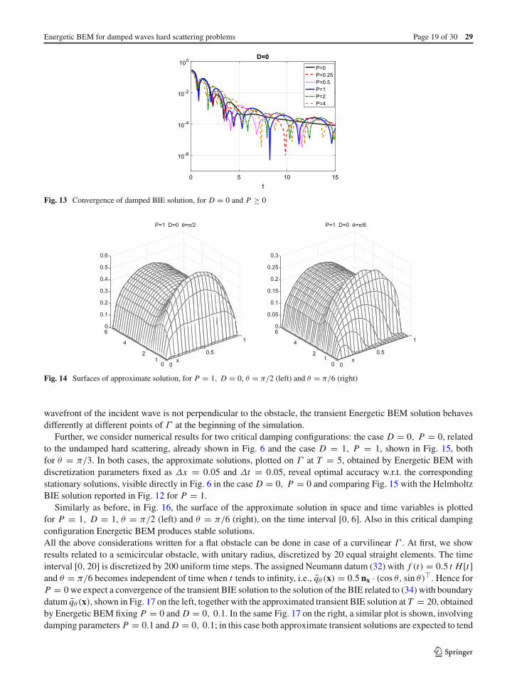
Looking at the graphs reporting the time history of ‖ϕ(·, t) − ϕ∞(·)‖L1(Γ ), shown in Fig. 13 for D = 0, P ≥ 0,we observe the expected convergence of each approximate transient solution to the corresponding approximatestationary one obtained using the same space discretization parameter. In particular, curves reveal a growing numberof oscillations for growing P > 0 (underdamping configuration), but the same global decay of the undamped case,which presents a monotone convergence after t = 6 time instant. Note that the oscillations are due to intersectionsbetween approximate transient solutions and corresponding approximate stationary ones; they can be interpretedas oscillations of diminishing amplitude of each damped solution around its own equilibrium configuration.

In Fig. 14, the surface of the approximate solution in space and time variables is plotted for P = 1, D = 0,θ = π/2 (left), and θ = π/6 (right), on the time interval [0, 6]. Also here there is the evidence that when the

123


0 5 10 15t

10-6

10-4

10-2

100D=0

P=0P=0.25P=0.5P=1P=2P=4

Fig. 13 Convergence of damped BIE solution, for D = 0 and P ≥ 0

0

0.5

1

0

2

4

60

0.1

0.2

0.3

0.4

0.5

0.6

x

P=1 D=0 θ=π/2

t0

0.5

1

0

2

4

60

0.05

0.1

0.15

0.2

0.25

0.3

x

P=1 D=0 θ=π/6

t

Fig. 14 Surfaces of approximate solution, for P = 1, D = 0, θ = π/2 (left) and θ = π/6 (right)

wavefront of the incident wave is not perpendicular to the obstacle, the transient Energetic BEM solution behavesdifferently at different points of Γ at the beginning of the simulation.

Further, we consider numerical results for two critical damping configurations: the case D = 0, P = 0, relatedto the undamped hard scattering, already shown in Fig. 6 and the case D = 1, P = 1, shown in Fig. 15, bothfor θ = π/3. In both cases, the approximate solutions, plotted on Γ at T = 5, obtained by Energetic BEM withdiscretization parameters fixed as Δx = 0.05 and Δt = 0.05, reveal optimal accuracy w.r.t. the correspondingstationary solutions, visible directly in Fig. 6 in the case D = 0, P = 0 and comparing Fig. 15 with the HelmholtzBIE solution reported in Fig. 12 for P = 1.

Similarly as before, in Fig. 16, the surface of the approximate solution in space and time variables is plottedfor P = 1, D = 1, θ = π/2 (left) and θ = π/6 (right), on the time interval [0, 6]. Also in this critical dampingconfiguration Energetic BEM produces stable solutions.All the above considerations written for a flat obstacle can be done in case of a curvilinear Γ . At first, we showresults related to a semicircular obstacle, with unitary radius, discretized by 20 equal straight elements. The timeinterval [0, 20] is discretized by 200 uniform time steps. The assigned Neumann datum (32) with f (t) = 0.5 t H [t]and θ = π/6 becomes independent of time when t tends to infinity, i.e., q̄θ (x) = 0.5nx · (cos θ, sin θ)�. Hence forP = 0 we expect a convergence of the transient BIE solution to the solution of the BIE related to (34) with boundarydatum q̄θ (x), shown in Fig. 17 on the left, together with the approximated transient BIE solution at T = 20, obtainedby Energetic BEM fixing P = 0 and D = 0, 0.1. In the same Fig. 17 on the right, a similar plot is shown, involvingdamping parameters P = 0.1 and D = 0, 0.1; in this case both approximate transient solutions are expected to tend

123


0 0.2 0.4 0.6 0.8 10

0.1

0.2

0.3

0.4

0.5

App

roxi

mat

e B

IE s

olut

ion

T=5, D=1, P=1

Fig. 15 ϕ(x, T ) on Γ for the critical damping configuration D = 1, P = 1, having fixed θ = π/3

0

0.5

1

0

2

4

60

0.1

0.2

0.3

0.4

0.5

x

P=1 D=1 θ=π/2

t0

0.5

1

0

2

4

60

0.05

0.1

0.15

0.2

0.25

0.3

x

P=1 D=1 θ=π/6

t

Fig. 16 Surfaces of approximate solution, for P = D = 1, θ = π/2 (left) and θ = π/6 (right)

0 0.5 1 1.5 2 2.5 3 parametrization interval

-0.2

0

0.2

0.4

0.6

0.8

1

P=0,D=0P=0,D=0.1Laplace BIE solution

0 0.5 1 1.5 2 2.5 3 parametrization interval

-0.2

0

0.2

0.4

0.6

0.8

1

P=0.1,D=0P=0.1,D=0.1

Fig. 17 Approximated transient BIE solutions for P = 0, D = 0, 0.1 and BIE static solution on Γ related to the Laplace BVP (34)(left), approximated transient BIE solutions for P = 0.1, D = 0, 0.1 (right), for θ = π/6 and T = 20

123


0 5 10 15 20t

0

0.2

0.4

0.6

0.8

1

P=0, D=0P=0, D=0.1

0 5 10 15 20t

0

0.2

0.4

0.6

0.8

1

P=0.1, D=0P=0.1, D=0.1

Fig. 18 Time history of Γ midpoint solution for P = 0, D = 0, 0.1 (left) and for P = 0.1, D = 0, 0.1 (right), for θ = π/6

Fig. 19 Behavior of the approximated transient solution on Γ in the first time instant of analysis (left) and for growing time (right),for P = 0.1, D = 0, and for θ = π/6

Fig. 20 Images of the last two curvilinear obstacles

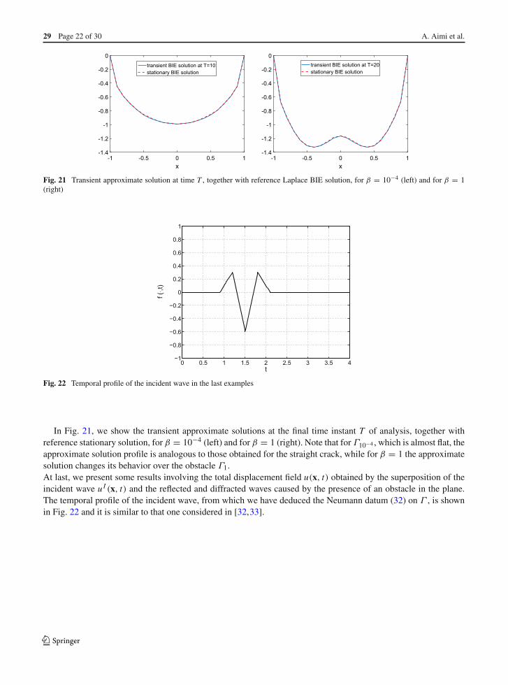
to the same stationary Helmholtz BIE solution over the semicircular arc. The overlapping is very good. In Fig. 18,the time history of Γ midpoint solution in the previous parameters case is presented. Note that for D = 0, transientsolution is still slightly oscillating, while damped solution has already reached a stationary configuration at the endof the time interval of analysis. At last, in Fig. 19, for P = 0.1, D = 0 we plot the behavior of the approximatedtransient solution on Γ in the first time instants of analysis on the left and for growing time on the right. Note thatfor t = 14 and t = 20 the graphs are nearly overlapped.

Now, fixing the temporal incident wave profile as f (t) = − 0.5 t H [t], let us consider the following obstacles:

Γβ = {x = (x, β sin(πx))|x ∈ [− 1, 1]} , β = 10−4, 1

whose images are reported in Fig. 20, stricken perpendicularly by the considered plane linear wave. These obstaclesare non-uniformly meshed by a uniform decomposition of the parametrization interval in 20 subintervals. Forβ = 10−4, the time interval of analysis [0, 10] is uniformly subdivided by using Δt = 0.1; for β = 1 the timeinterval of analysis is doubled as well as the number of time mesh intervals. Fixing P = 0, D = 0.01, we expectthat, for growing time, the approximate transient BIE solution tends to the corresponding Laplace BIE stationaryone, as happened in the previously analyzed cases.

123


-1 -0.5 0 0.5 1x

-1.4

-1.2

-1

-0.8

-0.6

-0.4

-0.2

0transient BIE solution at T=10stationary BIE solution

-1 -0.5 0 0.5 1x

-1.4

-1.2

-1

-0.8

-0.6

-0.4

-0.2

0transient BIE solution at T=20stationary BIE solution

Fig. 21 Transient approximate solution at time T , together with reference Laplace BIE solution, for β = 10−4 (left) and for β = 1(right)

0 0.5 1 1.5 2 2.5 3 3.5 4−1

−0.8

−0.6

−0.4

−0.2

0

0.2

0.4

0.6

0.8

1

t

f (⋅,t

)

Fig. 22 Temporal profile of the incident wave in the last examples

In Fig. 21, we show the transient approximate solutions at the final time instant T of analysis, together withreference stationary solution, for β = 10−4 (left) and for β = 1 (right). Note that for Γ10−4 , which is almost flat, theapproximate solution profile is analogous to those obtained for the straight crack, while for β = 1 the approximatesolution changes its behavior over the obstacle Γ1.At last, we present some results involving the total displacement field u(x, t) obtained by the superposition of theincident wave uI (x, t) and the reflected and diffracted waves caused by the presence of an obstacle in the plane.The temporal profile of the incident wave, from which we have deduced the Neumann datum (32) on Γ , is shownin Fig. 22 and it is similar to that one considered in [32,33].

123


Fig. 23 Total recovered displacement around breakwater obstacle for P = 0, D = 0

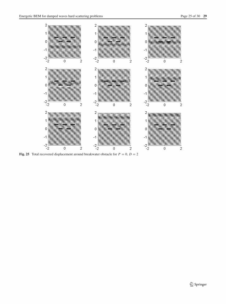
In the first simulation, Energetic BEM is applied in the case of a disconnected obstacle. In particular, the incidentplane wave strikes perpendicularly a breakwater obstacle, made by five disjoint aligned or parallel segments eachof length 0.5. The observation time interval is [0, 3]. As uniform temporal discretization step we use Δ t = 0.1 andevery segment is uniformly approximated by 5 boundary elements. The total recovered displacement in a squarearound the obstacle at time instants t = 0.2 + j 0.3, j = 0, . . . , 8 is presented in Fig. 23 for P = 0, D = 0. Theseresults show how the plane wave reaches the obstacle and how Γ degenerates the wavefront. Reflected waves areevident in the lower half of the square. As time increases, the wavefront recovers and the scattering effect causedby the obstacle on the plane wave diminishes. As one can see, the adopted approximation technique furnishessatisfactory results. In Figs. 24, 25, we show analogous results for P = 0, D = 1 and P = 0, D = 2, respectively:the higher the value of D, the lower the effects of reflection and diffraction around the disconnected obstacle. Thewavefront is, however, overall weakened.

123



The proposed methodology can handle also closed boundaries. In the following simulation, the same incidentplane wave strikes a unitary circle. The observation time interval is [0, 4]. As uniform temporal discretization stepwe use Δ t = 0.1 and the boundary of the circle is uniformly approximated by 80 straight boundary elements.Several snapshots related to the total recovered displacement in a square around the plane convex domain are shownin Fig. 26 for P = D = 0. In Fig. 27 for P = 1, D = 0, the positive material damping coefficient amplifies therecovering of the wavefront at the top of the circle, producing circular waves that are not present in the undampedcase. Further, in Fig. 28 related to the critical damping configuration P = 1, D = 1, the positive viscosity weakensall phenomena around the circle visible in the previous figure.

123



123


Fig. 26 Total recovered displacement around the circular obstacle for P = D = 0

123


Fig. 27 Total recovered displacement around the circular obstacle for P = 1, D = 0

123


Fig. 28 Total recovered displacement around the circular obstacle for P = 1, D = 1

6 Conclusions

We have considered the numerical solution of 2D damped wave propagation exterior problems equipped by Neumannboundary condition, which model hard scattering phenomena. A modified version of Energetic BEM has beenapplied, in order to take into account the non-analytical time integrability of the hypersingular damped kernel hereinvolved. The original version of this method was already considered in the case of undamped wave equations,revealing, also from theoretical point of view, its accuracy and stability. Numerical results obtained in the dampedscenario confirm that these properties are maintained in presence of dissipation. Next steps will involve BEM–FEMcoupling for this kind of model problems.

Acknowledgements This work has been partially supported by INdAM, Italy, through granted GNCS research projects.

Funding Open access funding provided by Università degli Studi di Parma within the CRUI-CARE Agreement.

Open Access This article is licensed under a Creative Commons Attribution 4.0 International License, which permits use, sharing,adaptation, distribution and reproduction in any medium or format, as long as you give appropriate credit to the original author(s)

123


and the source, provide a link to the Creative Commons licence, and indicate if changes were made. The images or other third partymaterial in this article are included in the article’s Creative Commons licence, unless indicated otherwise in a credit line to the material.If material is not included in the article’s Creative Commons licence and your intended use is not permitted by statutory regulation orexceeds the permitted use, you will need to obtain permission directly from the copyright holder. To view a copy of this licence, visithttp://creativecommons.org/licenses/by/4.0/.

References

1. Gaul L (1999) The influence of damping on waves and vibrations. Mech. Syst. Sign. Process. 13(1):1–302. Langer S (2004) BEM-studies of sound propagation in viscous fluids. In: ECCOMAS 2014 Conference Proceedings3. Mazzotti M, Bartoli I, Marzani A, Viola E (2013) A 2.5D boundary element formulation for modeling damped waves in arbitrary

cross-section waveguides and cavities. J. Comput. Physics 248(1):363–3824. Reinhardt A, Khelif A, Wilm M, Laude V, Daniau W, Blondeau-Patissier V, Lengaigne G, Ballandras S (2005) Theoretical analysis

of damping effects of acoustic waves at SOLID/FLUID interfaces using a mixed periodic FEA/BEM approach. In: EFTF 2005Conference Proceedings, pp. 606–610

5. Aimi A, Panizzi S (2014) BEM-FEM coupling for the 1D Klein-Gordon equation. Numer. Methods Partial Differential Equations30(6):2042–2082

6. Gaul L, Schanz M (1998) Material damping formulations in boundary element methods. In: IMAC 1998 Conference Proceedings7. Gaul L, Schanz M (1999) A comparative study of three boundary element approaches to calculate the transient response of

viscoelastic solids with unbounded domains. Computer Meth. Appl. Mech. Engrg. 179(1–2):111–1238. Vick A, West R (1997) Analysis of Damped Wave Using the Boundary Element Method. Trans. Modell. Simul. 15:265–2789. Abreu A, Carrer J, Mansur W (2008) Scalar wave propagation in 2D: a BEM formulation based on the operational quadrature

method. Eng. Anal. Bound. Elem. 27:101–10510. Mansur W, Abreu R, Carrer J, Ferro M (2002) Wave propagation analysis in the frequency domain: Initial conditions contribution.

In: C. Brebbia, A. Tadeu, V. Popov (eds.) Twenty-Fourth International Conference on the Boundary Element Method IncorporatingMeshless Solution Seminar, BEM XXIV, International Series on Advances in Boundary Elements, vol. 13, pp. 539–548

11. Bamberger A, Ha Duong T (1986) Formulation variationelle espace-temps pour le calcul par potential retardé de la diffractiond’une onde acoustique (I). Math. Methods Appl. Sci. 8:405–435

12. Bamberger A, Ha Duong T (1986) Formulation variationelle pour le calcul de la diffraction d’une onde acoustique par une surfacerigide. Math. Methods Appl. Sci. 8:598–608

13. Falletta S, Monegato G (2014) An exact non reflecting boundary condition for 2D time-dependent wave equation problems. Wavemotion 51(1):168–192

14. Givoli D (2004) High-order non-reflecting boundary conditions: a review. Wave motion 39:319–32615. Mossaiby F, Shojaei A, Booromand B, Zaccariotto M (2020) Local Dirichlet-type absorbing boundary conditions for transient

elastic wave propagation problems. Computer Meth. Appl. Mech. Engrg. 362:11285616. Shojaei A, Hermann A, Seleson P, Cyron C (2020) Dirichlet absorbing boundary conditions for classical and peridynamic diffusion-

type models. Comput. Mech. 66(4):773–79317. Shojaei A, Mossaiby F, Zaccariotto M, Galvanetto U (2019) A local collocation method to construct Dirichlet-type absorbing

boundary conditions for transient scalar wave propagation problems. Computer Meth. Appl. Mech. Engrg. 356:629–65118. Ha Duong T (2003) On retarded potential boundary integral equations and their discretization. In: P.D. et al. (ed.) Topics in

computational wave propagation. Direct and inverse problems, pp. 301–336. Springer-Verlag19. Costabel M (2004) Time-dependent problems with the boundary integral equation method. In: E. Stein (ed.) Encyclopedia of

Computational Mechanics, pp. 1–28. John Wiley and Sons20. Aimi A, Diligenti M, Panizzi S (2010) Energetic Galerkin BEM for wave propagation Neumann exterior problems. CMES

58(2):185–21921. Aimi A, Diligenti M (2008) A new space-time energetic formulation for wave propagation analysis in layered media by BEMs.

Internat. J. Numer. Methods Engrg. 75:1102–113222. Stephan E, Suri M (1989) On the convergence of the p-version of the Boundary Element Galerkin Method. Math. Comp. 52(185):31–

4823. Becache E (1993) A variational Boundary Integral Equation method for an elasodynamic antiplane crack. Internat. J. Numer.

Methods Engrg. 36:969–98424. Aleixo R, Capelas de Oliveir E (2008) Green’s function for the lossy wave equation. Rev. Bras. Ensino Fis 30(1):1–525. Sezginer A, Chew W (1984) Closed Form Expression of the Green’s Function for the Time-Domain Wave Equation for a Lossy

Two-Dimensional Medium. IEEE TRANS. AP 32:527–52826. Todorova G, Yordanov B (2000) Critical exponent for a nonlinear wave equation with damping. C. R. Acad. Sci. Paris 330:557–56227. Hairer E, Lubich C, Schlichte M (1985) Fast numerical solution of nonlinear Volterra convolution equations. SIAM J. Sci. Stat.

Comput. 6:532–54128. Aimi A, Diligenti M, Guardasoni C (2010) Numerical integration schemes for space-time hypersingular integrals in Energetic

Galerkin BEM. Num. Alg. 55(2–3):145–170

123

http://creativecommons.org/licenses/by/4.0/


29. Monegato G, Scuderi L (1999) Numerical integration of functions with boundary singularities. J. Comput. Appl. Math. 112(1–2):201–214

30. Aimi A, Diligenti M, Monegato G (1997) New numerical integration schemes for applications of Galerkin BEM to 2-D problems.Internat. J. Numer. Methods Engrg. 40:1977–1999

31. Diligenti M, Monegato G (1993) Finite-part integrals: their occurence and computation. Rendiconti del Circolo Matematico diPalermo, Series II(33):39–61

32. Iturraran-Viveros U, Vai R, Sanchez-Sesma FJ (2005) Scattering of elastic waves by a 2-D crack using the Indirect BoundaryElement Method (IBEM). Geophys. J. Int. 162:927–934

33. Sanchez-Sesma FJ, Iturraran-Viveros U (2001) Scattering and diffraction of SH waves by a finite crack: an analytical solution.Geophys. J. Int. 145:749–758

Publisher’s Note Springer Nature remains neutral with regard to jurisdictional claims in published maps and institutional affiliations.

123

Documents

Energetic boundary element method for accurate solution of