Enemalta FMA Draft Final Report 2010-11-19 · PDF fileENVIRONMENTAL ASSESSMENT OF THE INVESTMENT OPTIONS 32 ... REVIEW OR USE OF THIS REPORT ... Relative Dependence of the Options

Report

Fuel Optimization Study

to

Enemalta

November 12 2010

Fuel Optimization Study

to

Enemalta

IPA Energy + Water Economics Limited 101 Wigmore Street London W1U 1QU

United Kingdom Tel: +44 (0) 20 7962 1333 Fax: +44 (0) 20 7962 1321

Email: [email protected] Web site: www.ipaeconomics.com

TABLE OF CONTENTS

TABLE OF CONTENTS

DISCLAIMER I

GLOSSARY II

LIST OF EXHIBITS III

1. EXECUTIVE SUMMARY 4

2. INTRODUCTION 7

3. MODELLING APPROACH 9

4. MODEL ASSUMPTIONS 11

4.1. Macroeconomic Assumptions 11 4.2. Energy and Peak Demand Projections 11 4.3. Characteristics of Existing Power Plants 12 4.4. Characteristics of New (Potential) Plants 13 4.5. Characteristics of Interconnectors 15 4.6. International Fuel Price Projections and Scenarios 17 4.7. Southern Italian Power Prices and Scenarios 19 4.8. CO2, SO2 and NOx Emissions 20 4.9. SO2 and NOX Emission Abatement 22 4.10. Costs Associated with the Emissions of CO2, SO2 and NOx 23

5. MODEL SCENARIOS 26

5.1. The Core Scenarios 26 5.2. The Additional Scenarios 26

6. FINANCIAL ASSESSMENT OF THE INVESTMENT OPTIONS 28

6.1. NPVSC under Core Scenarios 28 6.2. NPVSC under Additional Scenarios 29 6.3. Levelised Cost of Power (LCP) under Core Scenarios 30 6.4. Levelised Cost of Power (LCP) under Additional Scenarios 30 6.5. Conclusions Based on Financial Measures 31

7. ENVIRONMENTAL ASSESSMENT OF THE INVESTMENT OPTIONS 32

7.1. CO2 Emissions under Core Scenarios 32 7.2. CO2 Emissions under Additional Scenarios 32 7.3. SO2 Emissions under Core Scenarios 33 7.4. SO2 Emissions under Additional Scenarios 34 7.5. NOx Emissions under Core Scenarios 35 7.6. NOx Emissions under Additional Scenarios 36 7.7. Conclusions Based on Environmental Measures 36

8. QUALITATIVE ASSESSMENT OF THE INVESTMENT OPTIONS 37

8.1. New Capacity Requirements under Core Scenarios 37 8.2. New Capacity Requirements under Additional Scenarios 38 8.3. Analysis of Fuel Storage Requirements 41 8.4. Analysis of Security of Supply Issues 42

9. CONCLUSIONS 44

ANNEX A : EXPLANATION OF PLANT CHARACTERISTICS 46

ANNEX B: OPTIMAL NEW BUILD CAPACITY 47

ANNEX C: INVESTMENT MODEL MAINTENANCE AND EXTENSION S 48

TABLE OF CONTENTS

The Investment Model 48 Maintenance Issues 49 Potential Extensions 49

ANNEX D: INTRODUCTION TO THE ECLIPSE ® PLATFORM 52

DISCLAIMER

i

IMPORTANT NOTICE REVIEW OR USE OF THIS REPORT BY ANY PARTY CONSTITUTES ACCEPTANCE OF THE FOLLOWING TERMS. Please read these terms carefully. They constitute a binding agreement between you and IPA Energy + Water Economics Limited (“IPA”). By your review or use of the report, you hereby agree to the following terms. Use of this Report This Report is prepared for Enemalta Corporation (the “Client”). Use of this Report without this disclaimer is forbidden. The Client may refer to this Report and information contained within for reporting and research purposes, which may be shared with third parties for their internal use only and such use shall be governed by the terms contained in this notice as stated here. Distribution of this Report Only the Client may copy this report in whole or in part to relevant government ministry or bodies in Malta for their internal use only and such use shall be governed by the terms contained in the notice as stated here. Content of this Report This report and information and statements herein are based in whole or in part on information obtained from various sources. IPA makes no assurances as to the accuracy of any such information or any conclusions based thereon. IPA is not responsible for typographical, pictorial or other editorial errors. The report is provided AS IS. Warranties NO WARRANTY, WHETHER EXPRESSED OR IMPLIED, INCLUDING THE IMPLIED WARRANTIES OF MERCHANTABILITY AND FITNESS FOR A PARTICULAR PURPOSE IS GIVEN OR MADE BY IPA IN CONNECTION WITH THIS REPORT. You use this report at your own risk. IPA is not liable for any damages of any kind attributable to your use of this report.

DISCLAIMER

GLOSSARY

ii

GLOSSARY

ACF Annual Capacity Factor BAT Best Available Techniques / Technologies CAPEX Capital Expenditure CCGT Combined Cycle Gas Turbine CDM Clean Development Mechanism CO2 Carbon Dioxide ECLIPSE Emission Constraints and Policy Interactions in Power System Economics ELV Emission Limit Values EU ETS European Union Emissions Trading Scheme FOM Fixed Operating and Maintenance GHG Greenhouse Gases GWh Gigawatt-hour HFO Heavy Fuel Oil HHV Higher Heating Value HVAC High Voltage Alternating Current IMF International Monetary Fund IPPC Integrated Pollution Prevention and Control IED Industrial Emissions Directive JI Joint Implementation KWh Kilowatt Hour LCPD Large Combustion Plant Directive LRCCR Levelised Real Capital Charge Rate LNG Liquefied Natural Gas MW Megawatt MWh Megawatt-hour NERP National Emission Reduction Plan NPV Net Present Value NOx Nitrogen Oxide OCGT Open Cycle Gas Turbine PV Present Value SO2 Sulphur Dioxide ToP Take or Pay VOM Variable Operating and Maintenance WEO World Economic Outlook

LIST OF EXHIBITS

iii

LIST OF EXHIBITS

Exhibit 1: NPV of Total System Cost - Scenarios relative to Status Quo..................................... 5 Exhibit 2: Total Energy and Peak Demand Projections.............................................................. 12 Exhibit 3: Characteristics of Existing Generation Capacity........................................................ 13 Exhibit 4: Characteristics of Firm Build Plants........................................................................... 14 Exhibit 5: Characteristics of New Build Plants........................................................................... 15 Exhibit 6: Characteristics of the Firm Build Interconnector ....................................................... 16 Exhibit 7: Characteristics of the New Build Interconnector ....................................................... 16 Exhibit 8: Base Case Fuel Price Scenarios.................................................................................. 18 Exhibit 9: Low Case Fuel Price Scenarios .................................................................................. 18 Exhibit 10: High Case Fuel Price Scenarios ............................................................................... 18 Exhibit 11: Hourly Weekday Power Prices in Southern Italy..................................................... 19 Exhibit 12: Hourly Weekend Power Prices in Southern Italy..................................................... 19 Exhibit 13: Southern Italy Power Price Escalation Factor .......................................................... 20 Exhibit 14: CO2 Content of Fuels ............................................................................................... 21 Exhibit 15: SO2 Content of Fuels................................................................................................ 21 Exhibit 16: NOx Intensity of Existing, Firm Build, and New Build Plants ................................ 22 Exhibit 17: Percentage Reduction in NOx .................................................................................. 23 Exhibit 18: CO2 Price Scenarios ................................................................................................. 24 Exhibit 19: 18 Core Scenarios Modelled .................................................................................... 26 Exhibit 20: Additional Scenarios Modelled ................................................................................ 27 Exhibit 21: NPVSCs - Core Scenarios Indexed to Scenario 1 (NPVSC under Scenario 1 = 100)..................................................................................................................................................... 28 Exhibit 22: NPVSCs - Additional Scenarios............................................................................... 29 Exhibit 23: LCPs - Core Scenarios Indexed to Scenario 1 (LCP under Scenario 1 = 100) ........ 30 Exhibit 24: LCPs - Additional Scenarios .................................................................................... 30 Exhibit 25: CO2 Emissions - Core Scenarios Indexed to Scenario 1 (Scenario 1 = 100) .......... 32 Exhibit 26: CO2 Emissions - Additional Scenarios.....................................................................32 Exhibit 27: SO2 Emissions - Core Scenarios Indexed to Scenario 1 (Scenario 1 = 100)............ 34 Exhibit 28: SO2 Emissions - Additional Scenarios .....................................................................34 Exhibit 29: NOx Emissions - Core Scenarios Indexed to Scenario 1 (Scenario 1 = 100) ........... 35 Exhibit 30: NOx Emissions - Additional Scenarios.....................................................................36 Exhibit 31: Optimal New Build Capacity – Core Scenarios ....................................................... 37 Exhibit 32: Optimal New Build Capacity – Lower Gasoil to HFO Price Ratio.......................... 39 Exhibit 33: Optimal New Build Capacity (2010-2035) – Additional 200 MW Interconnection 39 Exhibit 34: Optimal New Build Capacity (2010-2035) – Lower Italian Power Prices............... 40 Exhibit 35: Optimal New Build Capacity (2010-2035) – Higher Reserve Margin & Higher Gas Price Option. ............................................................................................................................... 41 Exhibit 36: Relative fuel storage requirements of the options .................................................... 42 Exhibit 37: Relative Dependence of Investment Options on External Sources and Countries... 43 Exhibit 38: Relative Dependence of the Options on One Commodity or Technology ............... 43 Exhibit 39: Overall Assessment of Investment Options ............................................................. 44

SECTION 1 EXECUTIVE SUMMARY

4

1. EXECUTIVE SUMMARY Enemalta Corporation (“Enemalta” or “the Client”) hired IPA Energy+Water Economics (“IPA”) to investigate options for future investment in generation and interconnection capacity in Malta to meet system requirements from demand growth and aging infrastructure, subject to volatile commodity prices in the future (“the Assignment”). Historically, heavy fuel oil and gasoil have been utilized for power generation in Malta. Without indigenous fossil fuel sources, the power system in Malta is dependent on imported fuels and hence susceptible to international prices which have fluctuated considerably within the last decade. This has prompted the authorities to plan for alternative thermal generation sources such as natural gas and also importing power. In parallel, the Client has recently decided to invest in a sub-sea HVAC cable of 1 x 200MW capacity to import electricity from Sicily. Enemalta is also interested in adding natural gas into its fuel mix for power generation, which can contribute to security of supply and help meet the future power demand and environmental goals at lower costs. Previous studies that IPA conducted for Enemalta emphasized the sensitivity of investment value in natural gas-fired local generation to differences in international fuel prices and volume of electricity imports from Sicily. This necessitated a deeper understanding of the dynamics that would underpin the optimal investment decisions. Thus, Enemalta commissioned IPA to undertake this Assignment, taking into consideration both financial and non-financial performance measures in assessing optimal investment decisions. As part of the Assignment, IPA has completed the following tasks:

� Construction of a comprehensive investment model that considers costs associated with each competing power generation option available and seeks to find the mixture of capacity and generation that would minimise the NPV of the total power system cost, given forecasted power demand and various predefined constraints over 2010-20351;

� Designing a series of scenarios in liaison with Enemalta to explore the potential impact of key drivers such as fuel prices and availability of natural gas in the power system;

� Assessment of the modelling results with respect to: financial performance, security of supply, dependence on one commodity or technology, and environmental performance.

This report sets out the assumptions, modelling results and analysis of various scenarios that the Client requested IPA to investigate. As required by the Client, the scenarios were devised in consideration of the investment decisions recently undertaken, especially the 1 x 200MW interconnector, to reflect three distinct investment decision paths to be analyzed:

1 IPA built the investment model for the purposes of the Assignment and also for Enemalta’s future use to assess different investment decisions.


5

1. Investment in gas import infrastructure given that 1 x 200MW Malta – Sicily interconnector will be built and commissioned in 2013;

2. No investment in gas import infrastructure given that 1 x 200MW Malta – Sicily interconnector will be built and commissioned in 2013; and

3. No investment in gas import infrastructure or interconnector – a hypothetical status quo scenario, since we are assuming that the decision to invest in the interconnector is already made – as a benchmark for comparison.

Each of the investment decision paths were modelled and analyzed under three fuel price (Base, Low, High) and two demand growth scenarios (Base, Low) resulting in 18 permutations. Modelling results show that the NPV of system costs are the lowest when gas is available except in the presence of low fuel prices. Findings on the relative financial performance of the scenarios with respect to the status quo are illustrated in the exhibit below.

Exhibit 1: NPV of Total System Cost - Scenarios relative to Status Quo

The investment options are also holistically assessed in terms of financial viability, environmental impact, fuel storage requirements and security of supply, resulting in the following conclusions. Investment in both the Interconnector and Gas Import Infrastructure - All Change Option: This option is associated with NPV of total system costs of between €3.4 billion to €5.7 billion. It scores relatively well on all metrics and is deemed to be the most attractive from the perspective of technology or commodity dependence.


6

Investment in the Interconnector without Investing in Gas Import Infrastructure – Environmentally Attractive Option: This option is associated with NPV of total system costs of between €3.3 billion to €6.0 billion. It appears to be the best in terms of both environmental performance (based on the metric of local rather than global emissions) and in fuel storage requirements. However, in terms of security of supply, it does not perform well, as a significant proportion of Malta’s energy supply would be dependent on a single country/interconnection point. No investment in Gas or an Interconnector - Status Quo Option: This option is associated with the highest NPV of total system costs which range between €3.6 and €6.9 billion depending on fuel prices and energy demand. Although this option does offer relatively less dependence on a single country than the other options, because it relies solely on the highly tradable commodity, oil, in terms of dependence on one commodity it scores badly. It also performs the least well on the other metrics - fuel storage requirement and environmental impact. Therefore, if possible, it is not recommended that the status quo should be maintained.

SECTION 2 INTRODUCTION

7

2. INTRODUCTION Enemalta Corporation (“Enemalta” or “the Client”) hired IPA Energy+Water Economics (“IPA”) to investigate options for future investment in generation and interconnection capacity in Malta to meet system requirements from demand growth and aging infrastructure, subject to volatile commodity prices in the future (“the Assignment”). Historically, heavy fuel oil and gasoil have been utilized for power generation in Malta. Without indigenous fossil fuel sources, the power system in Malta is dependent on imported fuels and hence susceptible to international prices which have fluctuated considerably within the last decade. This has prompted the authorities to plan for alternative thermal generation sources such as natural gas and also importing power. In parallel, the Client has recently decided to invest in a sub-sea HVAC cable of 1 x 200MW capacity to import electricity from Sicily. Enemalta is also interested in adding natural gas into its fuel mix for power generation, which can contribute to security of supply and help meet the future power demand and environmental goals at lower costs. Previous studies that IPA conducted for Enemalta emphasized the sensitivity of investment value in natural gas-fired local generation to differences in international fuel prices and volume of electricity imports from Sicily. This necessitated a deeper understanding of the dynamics that would underpin the optimal investment decisions. Thus, Enemalta commissioned IPA to undertake this Assignment, taking into consideration both financial and non-financial performance measures in assessing optimal investment decisions. As part of the Assignment, IPA has completed the following tasks:

� Construction of a comprehensive investment model that considers costs associated with each competing power generation option available and seeks to find the mixture of capacity and generation that would minimise the net present value of the total power system cost, given forecasted power demand and various predefined constraints over 2010-20352;

� Designing a series of scenarios in liaison with Enemalta to explore the potential impact of key drivers such as fuel prices and availability of natural gas in the power system;

� Assessment of the modelling results with respect to: financial performance, security of supply, dependence on one commodity or technology, and environmental performance.

This report sets out the assumptions, modelling results and analysis of various scenarios that the Client requested IPA to investigate. The scenarios considered the impact of the following factors:

� availability of gas � power demand � fuel prices (reference oil, gas, HFO, gasoil, carbon) � the existence of power interconnector(s) between Sicily and Malta

2 IPA built the investment model for the purposes of the Assignment and also for Enemalta’s future use to assess different investment decisions.

SECTION 2 INTRODUCTION

8

� gasoil to HFO price ratios � Italian power prices � the reserve margin requirement in the power system of Malta � gas purchase options (specific commercial terms).

In particular, the scenario results were assessed in terms of their: � financial performance � security of supply � fuel storage requirements � dependence on external sources and countries � dependence on one commodity or technology � environmental performance.

The remainder of this report is structured as follows:

� Section 3 explores the modelling methodology � Section 4 sets out the assumptions used in the scenario modelling � Section 5 provides details of the scenarios modelled � Section 6 sets out the modelling results � Section 7 analyses the results � Section 8 draws conclusions � Annex A explains the meaning of key plant characteristics � Annex B presents total new build capacity under different scenarios � Annex C provides a description of the model used and discusses maintenance

issues as well as potential extensions with respect to the model. � Annex D provides a short description of IPA’s ECLIPSE® modelling platform � Annex E includes the New Party Undertaking document

SECTION 3 MODELLING METHODOLOGY

9

3. MODELLING APPROACH In order to carry out the required analysis for the Assignment, IPA developed a 25-year electricity dispatch and investment assessment model, encompassing the period 2009-2035 (“the Investment Model” or “the Model”). The Investment Model is an implementation of IPA’s proprietary power market analysis platform, the ECLIPSE®. The underlying ECLIPSE® algorithm assesses alternative dispatch and capacity expansion patterns and selects the schedule that minimises the total operating and investment costs over the entire forecast horizon. ECLIPSE® therefore provides the resulting NPV of the total cost of power generation as well as power prices, and total pollutant emissions over the time period considered. This makes ECLIPSE® an attractive platform to produce the quantitative underpinnings of optimal options for the secure, clean, and cost-effective expansion of a power system that are also robust under various fuel price and growth scenarios3. The Investment Model has the following Key Features:

� Development in the Microsoft Excel Environment;

� Ability to define, develop and solve very complex mathematical programming challenges associated with electricity dispatch and capacity expansion modelling by the addition of a 3rd party complex linear optimiser, What’s Best;

� Development in a Windows-friendly environment enabling model results to be easily linked to other spreadsheets;

� Implementation of least-cost system dispatch modelling algorithm, dispatching generation units to meet demand and minimise the cost of system operation;

� Ability to limit dispatch subject to generator-specific constraints;

� Simulation of the hourly dispatch of the system for a typical weekday and weekend day for every month over the period 2009-2035;

� Simulation of the operation of each generation unit, along with its capacity, fuel costs, variable costs, and fixed costs;

� Ability to calculate the NPV impact of each investment option over the forecast horizon, taking into account all of the different cost components (all variable costs, fixed costs, capital costs) and their profile over the modelling period.

� Flexible enough to explore a vast number of scenarios based inter alia on the following variables:

o 3 different demand growth scenarios for peak and energy demand;

o 3 different price scenarios for 5 different commodities;

o 6 different evolution paths for 2 different Italian power price series;

o 2 different forecast bases for the reference natural gas prices;

o 6 different commercial arrangements for gas importation;

o option on whether natural gas is allowed in the system;

3 Please see Annex D for further information on the ECLIPSE® Platform.

SECTION 3 MODELLING METHODOLOGY

10

o option on whether CAPEX costs for Firm Build plants are captured as part of fixed costs of power generation

o options on various new capacity type, size and timing controls (i.e., which technology is allowed to come online after which year at which minimum and maximum magnitude)

SECTION 4 MODEL ASSUMPTIONS

11

4. MODEL ASSUMPTIONS The following sections set out the assumptions used in the analysis carried out for the Assignment. Unless explicitly stated in this report, the source of the assumptions is the Client and/or IPA’s own proprietary research. Over the course of the Assignment these assumptions have been revised and agreed with Enemalta through written and verbal correspondence.

4.1. Macroeconomic Assumptions

All macroeconomic variables enter the Investment Model as exogenous inputs and in real terms expressed in euro, chained to 2010 level.

FOREX

The euro-GB pound and US dollar-euro exchange rates are assumed to remain fixed over the forecast period at 0.87 and 0.75 respectively.

Inflation

It is assumed that the inflation rate in the Euro Area will increase substantially over the next six years from its current low level of 0.31% to 2% a year, where it is assumed to remain for the rest of the forecast period. The inflation rate forecast for the next 6 years is taken from the IMF October 2009 World Economic Outlook study. The inflation rate in the US is assumed to be 2% for the entire forecast period.

Discount Rate

Enamalta’s real discount rate of 6% is used to assess new investment options. It is implemented in the Investment Model as a fixed variable throughout the forecast horizon.

4.2. Energy and Peak Demand Projections

Annual energy demand (GWh) and peak demand (MW) are both assumed to grow at 1% per year in our base case scenario and 0.5% a year in our low case scenario.

Exhibit 2 illustrates how these assumptions affect the projections for electricity demand and peak demand. The reserve margin is currently assumed to be 20% but assumed to increase to 40% over the 2009-2014 period and remain at that level for the rest of the forecast period.


12

Exhibit 2: Total Energy and Peak Demand Projections

4.3. Characteristics of Existing Power Plants

It is assumed that current generating capacity, net of the plants’ own consumption and losses is 539.7MW. 74% of this capacity runs on HFO and the rest on gasoil (natural gas if / when available) as primary fuel. There are five generating plants, of which two are steam turbines, two are gas turbines, and one is a combined cycle gas turbine (CCGT). The two steam turbine plants are assumed to be decommissioned during the forecast period, one in 5 years (after 2013) and one in 12 years (after 2020). The CCGT plant is expected to be decommissioned in 17 years (after 2025). Exhibit 3, overleaf, summarises the characteristics of the existing power plants while Annex A provides further explanation.


13

Exhibit 3: Characteristics of Existing Generation Capacity

Plant Acronym: MPS_Steam MPS_GT DPS_Steam DPS_CCGT DPS_GT

Primary Fuel HFO 1% HFO 1% HFO 0.7% Gasoil Gasoil

Secondary Fuel HFO 1% Gasoil HFO0.7 Gas Gas

Size 204.20 36.5 120 107 72

Decommissioning Time (End of Year)

2013 N/A 2020 2026 N/A

Efficiency HHV 26.1% 32.0% 32.0% 40.0% 32.0%

Effective Forced Outage 10.0% 3.0% 2.0% 1.0% 3.0%

Scheduled Maintenance 4.6% 4.1% 8.2% 11.5% 4.1%

Minimum Availability Constraint

2.0% 11.0% 21.7% 18.7% 5.6%

FOM (€/KWy) 53.97 53.97 41.60 42.80 43.40

VOM4 (€/MWh) 0.34 0.34 0.11 0.11 0.11

Reserve Margin Contribution 90.0% 97.0% 98.0% 99.0% 97.0%

Maximum ACF 85.9% 93.0% 90.0% 87.6% 93.0%

Gas Conversion CAPEX (€/KW)

60 60 145 60 60

Gas Conversion Period (Modeling Years after 2008)

0 6 0 6 6

Retrofit Period N/A N/A 2011 N/A N/A

Retrofit CAPEX (€/KW) N/A N/A 198 N/A N/A

LRCCR For Gas Conversion and Retrofitting (% of CAPEX applied per annum)

26% 10% 17% 15% 10%

4.4. Characteristics of New (Potential) Plants

In our scenario modelling, two types of new plants are considered: those that are definitely going to be built (“Firm Build”) and those that could potentially be built (“New Build”) , if determined by the Investment Model as economically optimal. New Builds are added endogenously by the underlying ECLIPSE® algorithm, with the aim of minimising the costs of generating electricity whilst meeting peak and electricity demand. The decision of which technology, how much, and when to add to the power system is based on capital investment, financing, fuel, and other fixed and variable running costs for each New Build option.

4 Firm DPS_IC Plant incurs a VOM of 3.68 when gas is available for it to run and 8.28 otherwise. To be prudent regarding estimation of operating costs, New Diesel VOM is set to 8.28 regardless.


14

Firm Build Plants

In the Firm Build group, it is assumed that two 10MW solar power plants and one 144MW Internal Combustion plant will be built. All three plants are expected to come online in 4 years time (after 2012). Modelling assumptions regarding Firm Build plants are shown in the table below5.

Exhibit 4: Characteristics of Firm Build Plants

Plant Acronym: Firm Solar 1 Firm Solar 2 DPS_IC

Primary Fuel Solar Solar HFO0.7

Secondary Fuel Solar Solar Gas

Size 10 10 144

Online Year 2012 2012 2012

Life (Years) 25 25 99

Efficiency HHV 100.0% 100.0% 46.8%

Effective Forced Outage 5.0% 5.0% 3.0%

Scheduled Maintenance 0.0% 0.0% 5%

Minimum Availability Constraint 25.0% 25.0% 8.3%

FOM (€/KWy) 0.00 0.00 62.61

VOM (€/MWh) 300 250 3.68

Reserve Margin Contribution 30.0% 30.0% 97%

Maximum ACF 30.0% 30.0% 92.2%

CAPEX – Total Investment cost (€/KW) 0.0 0.0 955

LRCCR N/A N/A 8.44%

Gas Conversion CAPEX N/A N/A 191

Gas Conversion Period N/A N/A 6

LRCCR For Gas Conversion and Retrofitting

N/A N/A 10%

Note that the CAPEX for Firm Build solar plants is set to zero as Enemalta would not be incurring any of the investment costs. Instead, Government of Malta will finance the development and Enemalta would be required to purchase the power generated by these plants at the rates of €300/MWh and €250/MWh. This is effectively a variable operating cost for Enemalta. Therefore, these “feed-in” tariffs were modelled as if they were the VOM costs for the respective plants, incurred by Enemalta. LRCCR for gas conversion and retrofitting assumes that required return on capital is recovered during the plant’s operating life or the last modelling year, whichever comes first.

New Build Plants

The New Build plants include the following types6:

5 The model is also capable of modelling up to four other Firm Build plants, namely a Wind Powered plant, CHP plant and two other plants, which can be configured as desired. For the current runs however it was agreed that only DPS_IC, Interconnector (see next section), and two solar plants are modelled as Firm Build. 6 The Investment Model is also capable of investigating the viability of new wind plants as New Build. However, for the current model runs, this was not considered as per the Client’s request.


15

� Combined Cycle Gas Turbine (CCGT);

� Open Cycle Gas Turbine (OCGT);

� Diesel; and

� Solar

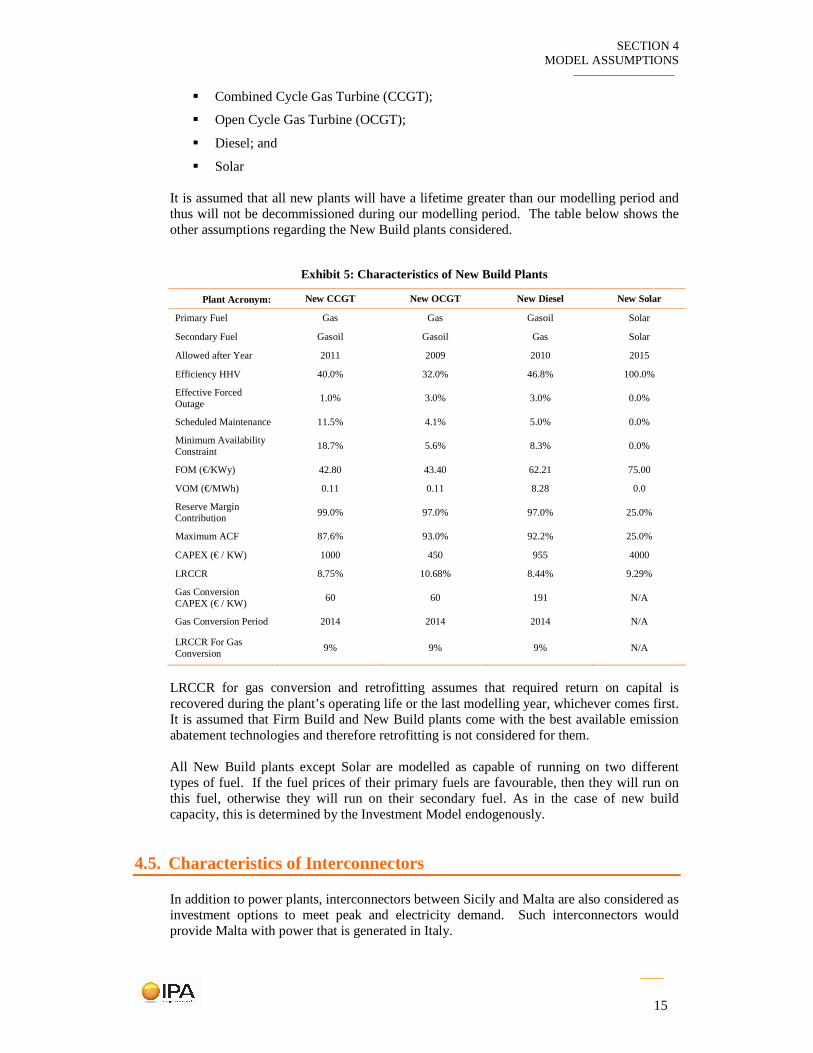
It is assumed that all new plants will have a lifetime greater than our modelling period and thus will not be decommissioned during our modelling period. The table below shows the other assumptions regarding the New Build plants considered.

Exhibit 5: Characteristics of New Build Plants

Plant Acronym: New CCGT New OCGT New Diesel New Solar

Primary Fuel Gas Gas Gasoil Solar

Secondary Fuel Gasoil Gasoil Gas Solar

Allowed after Year 2011 2009 2010 2015

Efficiency HHV 40.0% 32.0% 46.8% 100.0%

Effective Forced Outage

1.0% 3.0% 3.0% 0.0%

Scheduled Maintenance 11.5% 4.1% 5.0% 0.0%


18.7% 5.6% 8.3% 0.0%

FOM (€/KWy) 42.80 43.40 62.21 75.00

VOM (€/MWh) 0.11 0.11 8.28 0.0

Reserve Margin Contribution 99.0% 97.0% 97.0% 25.0%

Maximum ACF 87.6% 93.0% 92.2% 25.0%

CAPEX (€ / KW) 1000 450 955 4000

LRCCR 8.75% 10.68% 8.44% 9.29%

Gas Conversion CAPEX (€ / KW)

60 60 191 N/A

Gas Conversion Period 2014 2014 2014 N/A

LRCCR For Gas Conversion

9% 9% 9% N/A

LRCCR for gas conversion and retrofitting assumes that required return on capital is recovered during the plant’s operating life or the last modelling year, whichever comes first. It is assumed that Firm Build and New Build plants come with the best available emission abatement technologies and therefore retrofitting is not considered for them.

All New Build plants except Solar are modelled as capable of running on two different types of fuel. If the fuel prices of their primary fuels are favourable, then they will run on this fuel, otherwise they will run on their secondary fuel. As in the case of new build capacity, this is determined by the Investment Model endogenously.

4.5. Characteristics of Interconnectors

In addition to power plants, interconnectors between Sicily and Malta are also considered as investment options to meet peak and electricity demand. Such interconnectors would provide Malta with power that is generated in Italy.


16

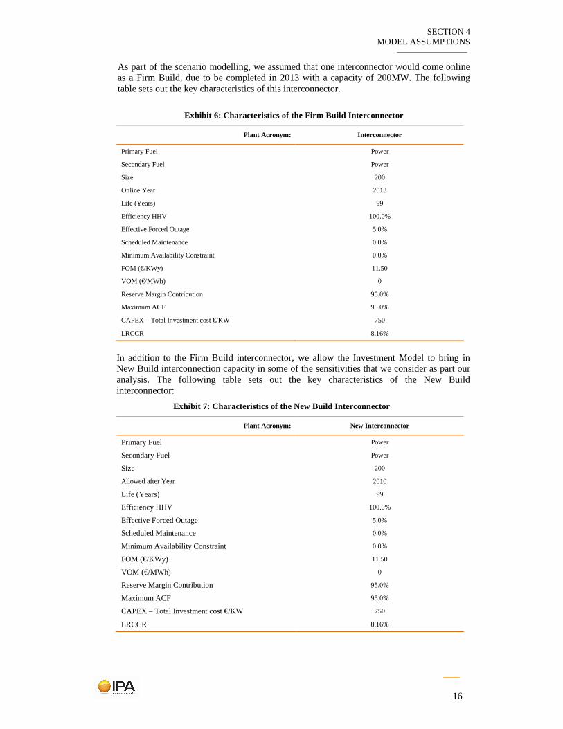
As part of the scenario modelling, we assumed that one interconnector would come online as a Firm Build, due to be completed in 2013 with a capacity of 200MW. The following table sets out the key characteristics of this interconnector.

Exhibit 6: Characteristics of the Firm Build Interc onnector

Plant Acronym: Interconnector

Primary Fuel Power

Secondary Fuel Power

Size 200

Online Year 2013

Life (Years) 99

Efficiency HHV 100.0%

Effective Forced Outage 5.0%

Scheduled Maintenance 0.0%

Minimum Availability Constraint 0.0%

FOM (€/KWy) 11.50

VOM (€/MWh) 0

Reserve Margin Contribution 95.0%

Maximum ACF 95.0%

CAPEX – Total Investment cost €/KW 750

LRCCR 8.16%

In addition to the Firm Build interconnector, we allow the Investment Model to bring in New Build interconnection capacity in some of the sensitivities that we consider as part our analysis. The following table sets out the key characteristics of the New Build interconnector:

Exhibit 7: Characteristics of the New Build Interconnector

Plant Acronym: New Interconnector

Primary Fuel Power

Secondary Fuel Power

Size 200

Allowed after Year 2010

Life (Years) 99

Efficiency HHV 100.0%

Effective Forced Outage 5.0%

Scheduled Maintenance 0.0%

Minimum Availability Constraint 0.0%

FOM (€/KWy) 11.50

VOM (€/MWh) 0

Reserve Margin Contribution 95.0%

Maximum ACF 95.0%

CAPEX – Total Investment cost €/KW 750

LRCCR 8.16%


17

4.6. International Fuel Price Projections and Scenarios

Four different fuel types were considered in our modelling:

� Heavy Fuel Oil with 0.7% Sulphur (“HFO0.7”)

� Heavy Fuel Oil with 1% Sulphur (“HFO1”);

� Gasoil (a.k.a diesel); and

� Natural Gas.

The charts overleaf present our base, low and high case delivered price assumptions for these fuels. These assumptions are based on IPA’s PowerView fuel price projections combined with a number of calibrations and comparisons with the delivered fuel prices Enemalta realised in 2009.

These three price scenarios have been designed to ensure that modelling results are robust under a range of fuel price scenarios.


18

Exhibit 8: Base Case Fuel Price Scenarios

Exhibit 9: Low Case Fuel Price Scenarios

Exhibit 10: High Case Fuel Price Scenarios


19

4.7. Southern Italian Power Prices and Scenarios

It was assumed that the cost of electricity sourced from the interconnector (Firm Build or New Build) would be equal to projected power prices in Southern Italy. The Southern Italian power price projections were calculated using average hourly power prices in Southern Italy for an average weekday and weekend in each month of 2009 and multiplying this price by an annual escalation factor to arrive at projections beyond 2009. Average hourly power prices in Southern Italy by month and workday/weekday as well as the calculated annual escalation factors are shown in the exhibits below.

Exhibit 11: Hourly Weekday Power Prices in Southern Italy

Exhibit 12: Hourly Weekend Power Prices in Southern Italy


20

Exhibit 13: Southern Italy Power Price Escalation Factor

The escalation factor used for modelling was the arithmetic average of the four other escalation factors, based on:

1. previous power price projections in Italy by IPA;

2. reference gas price projections used in this assignment;

3. reference oil price projections used in this assignment; and

4. reference carbon price projections used in this assignment.

As different reference fuel prices are assumed for different scenarios, the power price escalation factor is automatically adjusted and applied, resulting in a consistent change in the relative price of power coming through the interconnector.

We note that a commercial arrangement in the form of a long-term power purchase agreement via the interconnector is likely to result in more favourable power prices for Enemalta than spot prices. However, sufficient commercial detail had not been available for the purposes of modelling at the time the Assignment was undertaken.

4.8. CO2, SO2 and NOx Emissions

We considered the pollutant intensity of fuels and also power generation technologies to calculate the CO2, SO2 and NOx emissions that would be produced via power generation in Malta over 2009-2035. The following sub-sections describe the relevant assumptions used in the Investment Model in further detail.

CO2 Emissions

The following chart sets out the assumed CO2 intensity of the fuels (per MWh of fuel consumed) used in the modelling7.

7 These assumptions come from Table 1.4 in 2006 IPCC Guidelines for National Greenhouse Gas Inventories and Enemalta.


21

Exhibit 14: CO2 Content of Fuels

It is assumed that there are no emissions of CO2 associated with renewable generation plants, such as Solar. Similarly, it is also assumed that there are no emissions associated with power imported via the Interconnector. However, note that Enemalta will incur some CO2 emission costs for power produced in Italy when importing power through the Interconnector. These CO2 costs would be internalized in the Italian power prices

SO2 Emissions

The graph below shows the assumed SO2 content of Gasoil, HFO1, and HFO0.7.

Exhibit 15: SO2 Content of Fuels

Natural gas combustion produces negligible levels of SO2. Therefore, it is assumed that no emissions of SO2 would be produced via gas-firing. Likewise, power generation with renewables and power imports via the Interconnector are assumed to produce no SO2 emissions.


22

NOX Emissions

Emission of NOx are primarily determined by the generating plant characteristics rather than the fuel used. The following table sets out the NOx emissions associated with different generating plants. As in case of CO2 and SO2, renewables and interconnectors are not associated with NOx emissions.

Exhibit 16: NOx Intensity of Existing, Firm Build, and New Build Plants

4.9. SO2 and NOX Emission Abatement

With respect to SO2 abatement, it was assumed that the existing and new diesel plants would be able to abate nearly 80% of SO2 emissions produced during power generation. All other plants were assumed to emit SO2 in accordance with the SO2 content of the fuel used in the plant, shown in Section 4.8 above. With respect to NOx abatement, the following chart shows the percentage abatement expected to be achieved in the relevant plants, with respect to the NOx intensity levels presented in the previous section8.

8 Abatement level shown for DPS_CCGT and DPS_Steam are relevant for modelling period after 2011


23

Exhibit 17: Percentage Reduction in NOx

4.10. Costs Associated with the Emissions of CO2, SO2 and NOx

Although, Malta has no individual Greenhouse Gas (GHG) emission limitation commitments under the Kyoto Protocol, the Maltese Government is fully committed to reducing GHGs and as a Member State of the European Union, is bound by the obligations set out in the European Union legislation. There are a number of EU Regulations regarding the emission of CO2, SO2 and NOx that Malta is bound by. These regulations include:

� The EU’s Emission Trading Directive (2003/87/EC)

� The EU’s Large Combustion Plant Directive (LCPD, 2001/80/EC)

� The EU’s Integrated Pollution Prevention and Control Directive (IPPC, 2008/1/EC)

� The EU’s new Industrial Emissions Directive (IED)

Modelling the Cost of CO2 Emissions

The Emissions Trading Directive established the EU’s Emission Trading System (EU ETS). The scheme restricts the amount a carbon dioxide that can be emitted from certain energy intensive sectors, including power generation, by issuing a limited number of tradable permits that allows companies and industries to emit GHGs, which is primarily CO2. If organisations don’t have enough permits to cover their emissions, they must buy some permits, stop emitting or alternatively invest in a carbon reduction project outside Europe through the Clean Development Mechanism (CDM) or Joint Implementation scheme (JI) to offset their emissions. The EU ETS is currently in its second phase which runs from January 2008 to December 2012. The third phase will begin in January 2013. During the second phase, Member States determined (with the approval of the European Commission) how many allowances should be issued in their country. The final National Allocation Plan (NAP) approved by The European Commission allows 10.715 million tonnes of carbon credits


24

allocated to installations in Malta during the second phase of EU ETS. Under the NAP, no allocation of allowances will be made available up front to ‘new entrants’ in the power sector or in other sectors covered by the emissions trading scheme, unless the new entrants reserve is replenished through the transfer of allowances from an incumbent installation that undergoes full closure. In the absence of any allowances available in the reserve, new entrants will have to purchase the amount of allowances they require.Finally, injection of CDM/JI credits is allowed for up to 10% a level equivalent to 10% of the respective total allocation for each installation. From 2013, a single EU wide cap on emission allowances is envisaged to apply, reducing the number of allowances available to businesses to 21% below the 2005 level by 2020. The price of the tradable permits is determined by the market forces of demand and supply. CO2 emission reduction targets are not “physical”, i.e. they can simply be met by surrendering an adequate number of credits at the end of each compliance year based on actual emissions. Therefore, CO2 enters the Investment Model and subsequently our analysis as a variable cost based on power generated by local fossil fuel fired plants. The following chart sets out the carbon price projection assumptions that we used in our modelling. As with fuel costs, we investigated different scenarios using a Base, Low and High carbon price. These price projections are also from IPA’s Powerview publication.

Exhibit 18: CO2 Price Scenarios

0

10

20

30

40

50

60

70

80

Eu

ro /

To

nn

e

Base

Low

High

Modelling the Cost of SO2 and NOx Emissions

As for SO2 and NOx emissions, the LCPD applies to combustion plants with a thermal output greater than 50 MW. The directive states that all new combustion plants must comply with Emission Limit Values (ELV) as set out in the Annexes of the Directive. Older plants, those licensed prior to the 1st of July 1987, have three different options. They can either comply with the ELVs, operate within the emission trading scheme under the National Emissions Reduction Plan (NERP), or they can “opt out” from compliance


25

by committing to limit operations to no more than 20,000 operational hours between 1st January 2008 and 31 December 2015.

The IPPC introduced an environmental permit system that requires that all combustion installations with a thermal input rate exceeding 50MW must operate in such a way that:

a) All the appropriate preventative measures are taken against pollution, in particular through application of the best available techniques (BAT)

b) No significant pollution is caused

c) Waste production is avoided

d) Energy is used efficiently

e) Necessary measures are taken to prevent accidents and limit their consequences

f) the necessary measures are taken upon definitive cessation of activities to avoid any pollution risk and return the site of operation to a satisfactory state

The new IED, endorsed on the 7th of July 2010, combines seven existing air pollution directives, including the two abovementioned directives. It sets stricter limits on atmospheric pollutants such as nitrogen oxides (NOx) and sulphur dioxide (SO2) and dust. Installations will have until 2016 to comply with the stricter limits. However derogations will apply to Malta that will allow the installations to comply by 2020. Compliance will require implementation of “best available techniques”, or the most effective technologies that can provide high levels of environmental protection while balancing cost and benefit.

Regarding the existing plants in Malta only the 2x60MW steam plant is assumed to be relevant for retrofitting as others would either be decommissioned or would not require significant retrofitting to comply with the stricter limits of the IED. The steam plant is assumed to be retrofitted in 2011 with relevant abatement technologies at an estimated cost of €198 per KW.

As per new plants, the investment cost (capital expenditure) of each plant was assumed to include the cost of “best available technologies” and hence the cost of SO2 and NOx abatement is contained within the costs set out in section 4.4 above.

SECTION 5 MODEL SCENARIOS

26

5. MODEL SCENARIOS As per the Client’s requirements, IPA considered 18 core scenarios (“Core Scenarios”) for modelling and analysis. Based on the modelling results of the 18 Core Scenarios, the Client then requested that a further 7 scenarios (“Additional Scenarios”) are examined as sensitivities. Subsections below provide a detailed description of the 18 Core Scenarios and the 7 Additional Scenarios.

5.1. The Core Scenarios

Enemalta initially asked IPA to investigate how the introduction of the following three factors would affect optimal investment decisions in the power sector, under the three different fuel price scenarios as described in Section 4.6:

� a lower energy demand profile;

� a 200MW interconnector between Sicily and Malta; and

� availability natural gas.

To investigate the impact of these factors on the optimal investment decisions, IPA looked at the following 18 scenarios:

Exhibit 19: 18 Core Scenarios Modelled

With 200MW

Interconnector and Gas

With 200MW Interconnector and

Without Gas

No Interconnector and No Gas

Base Fuel Price Scenario1 Scenario 7 Scenario 13

Low Fuel Price Scenario 2 Scenario 8 Scenario 14 Baseline Energy Demand

High Fuel Price Scenario 3 Scenario 9 Scenario 15

Base Fuel Price Scenario4 Scenario 10 Scenario 16

Low Fuel Price Scenario 5 Scenario 11 Scenario 17

Low Energy Demand

High Fuel Price Scenario 6 Scenario 12 Scenario 18

5.2. The Additional Scenarios

The motivation behind investigating the Additional Scenarios was to better understand how some specific changes to the assumptions would affect the modelling results. In particular, Enemalta wished to see how the following factors would affect the results with respect to some of the Core Scenarios modelled:

� a lower gasoil to HFO price ratio;

� a compulsory second interconnector;

� lower Italian power prices;

SECTION 5 MODEL SCENARIOS

27

� a higher reserve margin;

� if Gas Option 1 rather than Gas Option 5, which represents a commercial arrangement yielding higher delivered gas prices, was taken.

The lower gasoil to HFO price ratio was applied to the aforementioned Scenario 8, while all other assumption changes were applied to Scenario 1. In the case of the compulsory second interconnector and the lower Italian power price, the changes were also introduced into Scenario 7 (i.e. Scenario 1 with no gas). The table below describes each of these additional scenarios in further detail.

Exhibit 20: Additional Scenarios Modelled

Scenario Acronym Description

1 8 HFOGO Scenario 8 (from the Core Scenarios) with Gasoil/HFO ratio set to 1.4 throughout the modelling timeline instead of the original variable that was set at 1.4 and rising to circa 1.7

2 CABL2 This is Scenario 1 (from the Core Scenarios) with a 200MW additional interconnector forced to come online in 2016. Also the reserve margin is adjusted to that there is at least 200MWs of reserve after the firm interconnector in 2013 is built.

3 CABL2NG As with CABL2 but without gas, i.e. Scenario 7.

4 LoPow This is Scenario 1 (from the Core Scenarios) with lower Italian power prices and the freedom for an additional interconnector to be built should it be deemed economical but with a maximum capacity of 120MW in any given year.

5 LoPowNG As with LoPow but without gas, i.e. Scenario 7.

6 ResMar This is Scenario 1 (from the Core Scenarios) where we adjust the reserve margin requirement to ensure that we have at least 200MWs of reserve after the Firm Build interconnector comes online.

7 S1GASOPT1 This is Scenario 1(from the Core Scenarios) with gas option 1 rather than option 5, in order to capture the impact of higher gas prices.

SECTION 6 FINANCIAL ASSESSMENT OF THE INVESTMENT OPTIONS

28

6. FINANCIAL ASSESSMENT OF THE INVESTMENT OPTIONS

This section sets out the financial assessment of the scenario analysis that IPA conducted based on the analysis of the Core Scenarios and Additional Scenarios modelled. In particular, we consider the relative costs of the options in terms of the net present value of the total system costs9 (NPVSC) and the Levelised Cost of Power (LCP).

6.1. NPVSC under Core Scenarios

The NPVSC for Scenario 1, where there is gas, a 200MW Interconnector, base fuel price and base energy demand is estimated to be approximately €4.6 billion. The NPVSC for the other scenarios relative to this scenario are shown in the table below.

Exhibit 21: NPVSCs - Core Scenarios Indexed to Scenario 1 (NPVSC under Scenario 1 = 100)

With 200MW



Without Gas


Base Fuel Price 100 103 115

Low Fuel Price 76 75 82 Base Energy

Demand

High Fuel Price 123 131 150


Low Fuel Price 75 73 78 Low Energy

Demand


These results show that, in general NPVSCs are the lowest in scenarios where there is gas in the system, except in the presence of a 200MW Interconnector and low fuel prices. Lower fuel prices in general favour generation with liquid fuels, resulting in a relatively lower consumption of gas in ideal conditions. However, the Take-or-Pay (ToP) conditions become binding in the presence of low fuel prices, pushing costs upwards and resulting in slightly less favourable total cost figures. When gas is not available, then a 200 MW Interconnector reduces NPVSCs by between 7.6% and 12.5% (i.e. comparing Scenario 13 to Scenario 7, Scenario 14 to Scenario 8 and Scenario 15 to Scenario 9).

Lower energy demand, could reduce NPVSCs by 2% to 5%. Impact of lower demand is greatest where total system costs are highest, i.e. in case of no gas and no Interconnector. The prevailing fuel price assumptions have the greatest impact on the overall system costs. Other things equal, the lower fuel prices could reduce NPVSCs by up to 29%, while the higher fuel prices could increase the same metric by up to 31% compared to the respective base fuel price scenario.

9 At a discount rate of 6% per annum.


29

6.2. NPVSC under Additional Scenarios

The following table summarises the NPVSCs of the Additional Scenarios and how they compare to the reference Core Scenarios (if other than Scenario 1) as well as to Scenario 1.

Exhibit 22: NPVSCs - Additional Scenarios

Scenario Acronym NPV of Total System

Cost (€000)

NPV of Total System Cost Indexed to relevant Scenario for comparison

NPV of Total System Cost Indexed to Scenario 1

(Scenario 1=100)

1 8 HFOGO 3,417,567 98 74

2 CABL2 4,765,754 Indexation to Scenario 1 - see figure in on the right

103

3 CABL2NG 4,783,188 101 103

4 LoPow 5,003,521 Indexation to Scenario 1 - see figure in on the right

108

5 LoPowNG 4,441,594 94 96

6 ResMar 4,646,660 Indexation to Scenario 1 - see figure in on the right

100

7 S1GASOPT1 5,113,334 Indexation to Scenario 1 - see figure in on the right

110

It appears that changing the gasoil to HFO price ratio to 1.4 (i.e., Scenario 8 HFOGO) results in a 2.1% reduction of the NPVSCs, relative to the respective base scenarios.

Forcing an additional 200MW interconnector in Scenario 1 (i.e., Scenario CABL2) leads to a 2.9% increase in NPVSC compared to Scenario 1. On the other hand, when a second interconnector is forcibly added in the absence of gas (i.e., Scenario CABL2NG), it increases the NPVSC by 3.2%, again with respect to Scenario 1, but has negligible impact (less than +1%) with respect to Scenario 7. The introduction of lower Italian power prices (i.e., Scenario LoPow) results in an 8% increase in NPVSC relative to Scenario 1. This is due to Take or Pay (ToP) constraints on natural gas10. When lower Italian power prices are introduced to Scenario 7 where no gas is allowed in the system (i.e., Scenario LoPowNG), NPVSC relative to Scenario 7 and Scenario 1 are lower by 6.49% and 4.1% respectively. Increasing the reserve margin (i.e., Scenario ResMar) yields a negligible increase (0.3%) in NPVSCs relative to Scenario 1.On the other hand, using Gas option 1 rather than Gas option 5 (i.e. Scenario S1GASOPT1) results in a 10% increase in NPVSC.

10 Without the ToP constraints, the NPVSC would be around 9% lower than in Scenario 1.


30

6.3. Levelised Cost of Power (LCP) under Core Scenarios

In addition to calculating the NPVSC, the Investment Model calculates the Levelised Cost of Power (LCP) which expresses the NPVSC in terms of Euros per megawatt hour generated. In Scenario 1, this cost is approximately €133 per MWh. The LCP associated with the other Core Scenarios relative to this scenario’s costs are presented in the table below.

Exhibit 23: LCPs - Core Scenarios Indexed to Scenario 1 (LCP under Scenario 1 = 100)

With 200MW Interconnector and Gas


Without Gas




Demand


Base fuel Price 102 102 114


Demand


As with NPSCs, levelised costs are generally at their lowest when there is gas available. However, levelised costs associated with low energy demand scenarios are slightly higher than the levelised costs associated with base energy demand scenarios. This is simply because in the low demand scenarios, although total system costs are lower as was seen in Section 6.1, costs in terms of megawatt hours generated are higher due to the proportionally lower volume of power generated.

6.4. Levelised Cost of Power (LCP) under Additional Scenarios

The following table summarises the LCPs of the Additional Scenarios and how they compare to the reference Core Scenarios (if other than Scenario 1) as well as to Scenario 1.

Exhibit 24: LCPs - Additional Scenarios

Scenario Acronym Levelised Cost

(€/MWh)

Levelised Cost indexed to relevant Scenario for

Comparison

Levelised Cost indexed to Scenario 1 (Scenario

1=100)

1 8 HFOGO 98 98 74

2 CABL2 137

Indexation to Scenario 1 - see figure in on the right 103

3 CABL2NG 138 101 103

4 LoPow 144


5 LoPowNG 128 94 96

6 ResMar 134


7 S1GASOPT1 147



31

Lowering the gasoil-HFO price ratio with respect to Scenario 8 lowers levelised costs by 2%.

On the other hand, forcibly introducing a second interconnector increases levelised costs by around 3% in scenarios where gas is available and around 1% in scenarios where gas is unavailable.

The introduction of lower Italian power prices, increases levelised costs when gas is available. Again this is due to the ToP conditions. When gas is unavailable, the lower Italian power prices reduce levelised costs by 6% relative to the same scenario and 4% relative to Scenario 1.

As with total NPVSCs, increasing the reserve margin only increases levelised costs slightly (0.3%) and changing the gas option to Option 1 rather than Option 5 increases levelised costs by around 10%.

6.5. Conclusions Based on Financial Measures

All in all, system costs are lower when gas is available, and energy demand as well as fuel prices are low. Of all factors affecting the total system costs, it is fuel prices that have the largest impact (c. 30% of swing when there is neither gas nor interconnection capacity). Bringing both gas and interconnection capacity jointly can pull down NPVSC by up to 18% (in the base demand and high fuel price case). Marginal impact of bringing gas or interconnection capacity separately into the energy mix is not assessed since investment in interconnection is already under way. Regardless, the results suggest that it is financially optimal to invest in gas import infrastructure.

SECTION 7 ENVIRONMENTAL ASSESSMENT OF THE INVESTMENT OPTIONS

32

7. ENVIRONMENTAL ASSESSMENT OF THE INVESTMENT OPTIONS

This section sets out the environmental assessment of the scenario analysis based on the Core Scenarios and Additional Scenarios. In particular, we consider the relative emissions of CO2, SO2 and NOx under different modelling scenarios.

7.1. CO2 Emissions under Core Scenarios

The total amount of CO2 to be emitted over the modelling period (2009-2035) under Scenario 1 is expected to be approximately 25 million tonnes. The CO2 expected to be emitted under different scenarios relative to Scenario 1 are presented in the following table:

Exhibit 25: CO2 Emissions - Core Scenarios Indexed to Scenario 1 (Scenario 1 = 100)

With 200MW



Without Gas




Demand High Fuel Price 100 94 161



Demand High Fuel Price 95 88 153

An interesting result is that when the Interconnector is present, the availability of gas actually increases CO2 emissions. The reason is that when gas is available, it is more cost effective to domestically generate power rather than importing through the Interconnector. Since no CO2 emissions are accounted for imported power, the scenarios without gas appear to result in lower emissions than the scenarios with gas when the Interconnector is present. Note that this does not mean that global carbon emissions are lower with the Interconnector. When the interconnector capacity and gas are not available and all power must be domestically generated with liquid fuels, CO2 emissions are significantly higher, as expected.

7.2. CO2 Emissions under Additional Scenarios

The table below summarises the CO2 emission results for the Additional Scenarios.

Exhibit 26: CO2 Emissions - Additional Scenarios

Scenario Acronym CO2 Emitted (2009-2035)

KTonnes

CO2 Emitted indexed to relevant scenario

CO2 Emitted indexed to Scenario 1 (Scenario 1=100)

1 8 HFOGO 26,251 103 105


33

2 CABL2 23,751


3 CABL2NG 23,106 95 92

4 LoPow 17,867


5 LoPowNG 19,301 80 77

6 ResMar 25,193


7 S1GASOPT1 23,699


Lowering the gasoil-HFO price ratio (with respect to Scenario 8) has interesting results. CO2 emissions tend to increase because as well as displacing HFO, the increased use of gasoil displaces power imports via the Interconnector. Since imported power is associated with zero (local) CO2 emissions, CO2 emissions originated from Malta increase.

The introduction of a second interconnector results in higher power imports compared to Scenario 1, reducing local CO2 emissions by 5%. The same trend is present no gas is available.

Lower power prices in Italy result in quite significant reductions in locally generated CO2, as lower prices make it more cost-effective to import power rather than producing domestically. Where gas is available the reduction is around 29% compared to the case where prices are higher (Scenario 7). In cases where gas is unavailable, the reduction in carbon is around 20% compared to Scenario 7. Increasing the reserve margin to 200MW does not have much impact on CO2 emissions but changing the gas purchasing option does result in lower local emissions. This is due to the fact that with higher gas prices, it is more cost effective to import power rather than generating it with gas.

7.3. SO2 Emissions under Core Scenarios

The total amount of SO2 emitted over the modelling period (2009-2035) under Scenario 1 is expected to be 40,000 tonnes. The amount of SO2 expected to be emitted in other scenarios relative to Scenario 1 is presented in the following table.


34

Exhibit 27: SO2 Emissions - Core Scenarios Indexed to Scenario 1 (Scenario 1 = 100)

With 200MW



Without Gas




Demand




Demand


Unlike CO2, local SO2 emissions are all lower when gas is available than when it is unavailable. The existence of the Interconnector does not change this result. Since gas generally contains negligible amounts of sulphur, the existence of gas in the generation mix quite significantly reduces the SO2 emissions. The Interconnector also reduces the amount of local SO2 emitted as we do not capture any emissions associated with imported power.

7.4. SO2 Emissions under Additional Scenarios

The table below summarises the SO2 emission results for the Additional Scenarios.

Exhibit 28: SO2 Emissions - Additional Scenarios

Scenario Acronym

SO2 Emitted (2009-2035) KTonnes

SO2 Emitted indexed to relevant scenario

SO2 Emitted indexed to Scenario 1 (Scenario

1=100)

1 8 HFOGO 63 92 157

2 CABL2 40 Indexation to Scenario 1 - see figure in on the right

100

3 CABL2NG 64 100 158

4 LoPow 41 Indexation to Scenario 1 - see figure in on the right

101

5 LoPowNG 54 84 133

6 ResMar 40 Indexation to Scenario 1 - see figure in on the right

100

7 S1GASOPT1 41 Indexation to Scenario 1 - see figure in on the right

101

Lowering the gasoil-HFO ratio results in lower local SO2 emissions with respect to Scenario 8. Lowering the price of gasoil, which is less SO2 intensive, makes it a more attractive fuel for electricity production, increasing its utilisation which results in lower SO2 emissions. However, local SO2 emissions are much higher compared to Scenario 1, as lower fuel prices make local power generation (versus importing) more attractive in general, which yields higher local SO2 emissions.


35

The introduction of a second 200 MW interconnector does not significantly affect local SO2 emissions because SO2 is only emitted from existing plants until the point where abatement technologies are introduced, with the vast majority of the local SO2 emissions within 2009-2035 emitted before the Firm Build Interconnector comes online. The second interconnector displaces generation plants that are virtually “SO2 free”, so its introduction has little effect on the local SO2 emissions. Lower Italian power prices actually cause a slight increase (1%) in local SO2 emissions when gas is available. This is because a small New OCGT plant (c. 33MW) is brought into the system by the Investment Model under this scenario in year 2010 as opposed to the 2 new plants, one New OCGT (15MW) and one New Diesel (18MW) as in Scenario 1. The reason for the difference in new build capacity is that OCGTs are cheaper to build but more expensive to run, making them better suited for meeting capacity demand rather than energy demand. When lower prices are introduced for imported power, power imports increase, reducing the energy demand that needs to be met via local generation. Therefore, the Investment Model favours the New OCGT over New Diesel. However, when the less efficient New OCGT does operate, it ends up emitting relatively larger amounts of SO2. When lower Italian power prices are introduced in the absence of gas, local SO2 emissions tend to fall by 16%. This is because more power is purchased from the Interconnector which displaces power generated through existing gas turbine and diesel plants that would have been utilised more, had power prices been higher. Increasing the reserve margin to 200MW does not have a significant impact on local SO2

emissions. Changing the gas purchase option results in a negligible increase in SO2 emissions.

7.5. NOx Emissions under Core Scenarios

In Scenario 1, total local NOx emissions over the modelling period (2009-2035) are expected to be around 59,000 tonnes. The expected local NOx emissions under different scenarios relative to Scenario 1 are presented in the table below.

Exhibit 29: NOx Emissions - Core Scenarios Indexed to Scenario 1 (Scenario 1 = 100)

With 200MW



Without Gas



Low Fuel Price 98 86 140 Base Energy Demand



Low Fuel Price 93 81 134 Low Energy Demand


Local NOx emissions are lowest when the Interconnector is present and gas is unavailable. This is because under such scenarios, more power is imported through the Interconnector, which provides imported power that is not associated with local NOx

emissions. When gas is available, it is cost effective to generate more power locally, resulting in higher local NOx emissions.


36

7.6. NOx Emissions under Additional Scenarios

The table below summarises the NOx emissions for with the Additional Scenarios.

Exhibit 30: NOx Emissions - Additional Scenarios

Scenario Acronym

NOx Emitted (2009-2035)

KTonnes

NOx Emitted indexed to relevant scenario

NOx Emitted indexed to Scenario 1 (Scenario

1=100)

1 8 HFOGO 52 102 88

2 CABL2 57 Indexation to Scenario 1 - see figure in on the right

96

3 CABL2NG 45 95 76

4 LoPow 41 Indexation to Scenario 1 - see figure in on the right

70

5 LoPowNG 37 78 63

6 ResMar 60 Indexation to Scenario 1 - see figure in on the right

101

7 S1GASOPT1 56 Indexation to Scenario 1 - see figure in on the right

94

When the gasoil to HFO price ratio is lowered with respect to Scenario 8, the lower priced fuels induce more local power generation and less import via the interconnector, increasing NOx emissions. The introduction of a second cable results in lower local NOx emissions both in scenarios with gas and scenarios without gas. This is because more power is sourced from the “NOx free” interconnectors at the expense of local generation. The same is true in scenarios where Italian power prices are lower (both LoPow and LoPowNG) and where gas prices are higher (S1GASOPT1). Increasing the reserve margin leads to a negligible increase in local NOx emissions.

7.7. Conclusions Based on Environmental Measures

The modelling results show that emissions are the lowest in scenarios where there is an interconnector, energy demand is low and fuel prices are high. In the case of CO2 and NOx emissions, availability of gas tends to increase emissions while lower Italian power prices induce the opposite. The reason that CO2 emissions are lower without gas or with lower Italian power prices is because less power is generated locally. Since we are considering locally produced emissions only, overall emissions of CO2 are lower when local generation falls. The reason that NOx emissions are lower when there is no gas is also partly because local generation is higher, but also because the availability of gas results in a greater capacity of new (local) plants that yield more NOx. In contrast, the availability of gas results in lower SO2 emissions. This is because gas-fired power generation is not associated with SO2, even though it increases the attractiveness of local generation. Existence of gas reduces generation with other fuels, which are more SO2 intensive.

SECTION 8 QUALITATIVE ASSESSMENT OF THE INVESTMENT OPTIONS

37

8. QUALITATIVE ASSESSMENT OF THE INVESTMENT OPTIONS

This section sets out the type and amount of new generation capacity that would need to be built under each of the scenarios modelled and then goes on to qualitatively assess the results in terms of:

• fuel storage requirements; and,

• security of supply.

The assessment of security of supply encompasses:

• dependence on external sources and countries; and,

• dependence on one commodity/technology.

8.1. New Capacity Requirements under Core Scenarios

The following chart shows the optimal new capacity under each of the Core Scenarios as determined by the Investment Model. Note that for scenarios where gas was present in the fuel mix (scenarios 1-6), it was found to be the strategic fuel of choice in terms of total fuel consumption in MWhs over the modelling period (2009-2035).

Exhibit 31: Optimal New Build Capacity – Core Scenarios

0

50

100

150

200

250

300

350

400

450

500

1 2 3 4 5 6 7 8 9 10 11 12 13 14 15 16 17 18

MW

New CCGT New OCGT New Diesel New Solar


38

Analysis Based on Gas and Firm Build Interconnector Availability

The results show that in scenarios where there is a 200MW Interconnector (scenarios 1-12), total new build capacity is lower than in scenarios where there is no interconnector. New Build capacity could be as low as 200MW if energy demand is low, but otherwise the system would need new capacity of around 250MW.

In scenarios where gas is available (scenarios 1-6) the Investment Model suggests a mix of New CCGT, New OCGT and New Diesel for additional capacity needs, with New Diesel dominating unless fuel prices are low. When fuel prices are low, New CCGTs that run on gas or gasoil are attractive enough to replace New Diesels that run on HFO or gas, depending on fuel availability and prices.

Where gas is unavailable, the Investment Model suggests that new capacity should largely come from New OCGT and New Diesel plants. In two of the scenarios where fuel prices are high and the Interconnector is not present (Scenarios 15 and 18), small amounts of New Solar capacity are also suggested. The optimal choice of new build capacity is also affected by fuel prices significantly. In scenarios where fuel prices are lower, New Diesel plants are favoured. In scenarios where fuel prices are higher, New CCGTs is preferred in scenarios where there is gas, while OCGT is favoured in scenarios where there is no gas.

8.2. New Capacity Requirements under Additional Scenarios

Lower Gasoil-HFO Price Ratio – Scenario 8HFOGO

The impact of changing the gasoil to HFO price ratio to 1.4 with respect to Scenario 8 is slightly larger New Diesel capacity and slightly smaller New OCGT capacity. This is due to the fact that New Diesel is cheaper to run compared to New OCGT, but more expensive to build. Whilst the lower gasoil price induces more New Diesel build, it also results in the higher utilisation of the existing DPS_GT plant. So, instead of completely replacing New OCGT in favour of New Diesel, the Investment Model finds the mix of new build and loading of new and existing plants that minimize the present value of total cost across the modelling period.


39

Exhibit 32: Optimal New Build Capacity – Lower Gasoil to HFO Price Ratio

0

50

100

150

200

250

300

Scenario 8 8 HFOGO

MW

New OCGT New Diesel

Additional Interconnector Build – Scenarios CABL2 and CABL2NG

Forcing a second 200MW interconnector into Scenario 1, affects the volume of new build capacity required as well as the plant choice of that build. This can be seen in the chart below.

Exhibit 33: Optimal New Build Capacity (2010-2035) – Additional 200 MW Interconnection

0

50

100

150

200

250

300

350

400

Scenario 1 CABL2 Scenario 7 CABL2NG

MW

New CCGT New OCGT New Diesel New Interconnection

The Investment Model suggests that when a second interconnector is added to new build capacity, total new build capacity increases to 336MW when gas is available and 301MW when gas is unavailable. This suggests that additional interconnection of 200MW in forced to come online in 2016 is redundant, at least partly, regardless of whether gas is in


40

the system. Utilization figures for the first 200MW and additional interconnection also support this finding. In case of CABL2 where gas is available, the utilisation of the first 200MW interconnector fluctuates between 33% and 60%, stabilising at around 45% by 2028. In case of CABL2NG where gas is not available, utilisation of the first 200MW interconnector is around 60% for the first few years, rising to 70% in 2021 and then stabilising around 80% by 2028. Utilisation of the additional 200 MW interconnection brought after 2016 is negligible in either case.

With respect to the capacity mix, introduction of the additional 200MW interconnector in scenarios with gas implies that only half the New Diesel capacity should be built and that no New CCGT or New OCGT should be built over 2010-2035. When gas is removed from this scenario, the results suggest that an even smaller diesel capacity (c.18MW) and OCGT capacity (c.38MW) would be optimal over 2010-2035. It also suggests that a slightly larger interconnector (c. 45MW) built in 2010 would have been optimal.

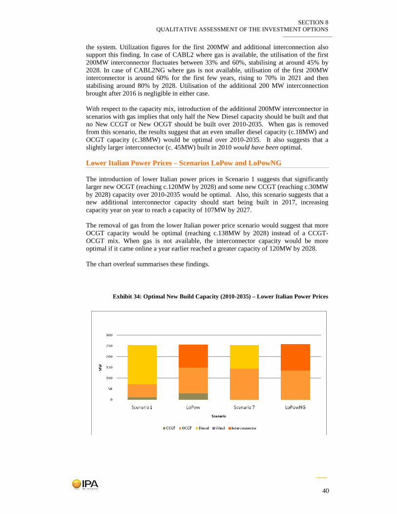
Lower Italian Power Prices – Scenarios LoPow and LoPowNG

The introduction of lower Italian power prices in Scenario 1 suggests that significantly larger new OCGT (reaching c.120MW by 2028) and some new CCGT (reaching c.30MW by 2028) capacity over 2010-2035 would be optimal. Also, this scenario suggests that a new additional interconnector capacity should start being built in 2017, increasing capacity year on year to reach a capacity of 107MW by 2027. The removal of gas from the lower Italian power price scenario would suggest that more OCGT capacity would be optimal (reaching c.138MW by 2028) instead of a CCGT-OCGT mix. When gas is not available, the interconnector capacity would be more optimal if it came online a year earlier reached a greater capacity of 120MW by 2028. The chart overleaf summarises these findings.

Exhibit 34: Optimal New Build Capacity (2010-2035) – Lower Italian Power Prices


41

Higher Reserve Margin and Higher Gas Prices – Scenarios ResMar and S1GASOPT

Increasing the reserve margin increases the total new build capacity that should be installed to 295MW and implies that it CCGT and OCGT capacity should be increased by 11% and 73% respectively compared to Scenario 1 and that diesel capacity should be reduced by slightly (2%). This result is presented in the chart below alongside the result that when the gas purchase option is changed, relatively more diesel capacity should be built at the expense of the OCGT capacity.

Exhibit 35: Optimal New Build Capacity (2010-2035) – Higher Reserve Margin & Higher Gas Price Option.

8.3. Analysis of Fuel Storage Requirements

Fuel storage requirements are less in scenarios where there are interconnectors than in those without interconnectors because less generation needs to be done locally reducing the need to store fuel. Also, the scenarios where liquid fuels are utilised locally imply higher fuel storage requirements. In case of gas, storage depends on the means of delivery. Pipeline and CNG deliveries are conceivable without any storage requirements, while LNG deliveries often require storage. Gas is therefore deemed to be the “middle” ranked option in terms of fuel storage requirements. The higher the energy demand, the larger the amount of fuel that will have to be stored, hence in lower energy demand scenarios, there will be less fuel storage requirements. The table below summarises these findings by ranking the scenarios according to the fuel storage requirements.


42

Exhibit 36: Relative fuel storage requirements of the options

With 200MW



Without Gas


Base fuel Price Low Fuel Price

Base Energy Demand

High Fuel Price Base fuel Price Low Fuel Price Low Energy

Demand High Fuel Price

Best Worst

8.4. Analysis of Security of Supply Issues

The assessment of security of supply encompasses the treatment of the following issues:

• dependence on external sources and countries; and,

• dependence on one commodity/technology.

The following subsections describe the analysis in detail.

8.4.1. Dependence on External Sources and Countries

To some degree Malta will always be dependent on external sources and countries. Oil and gas will always need to be imported as there is no domestic supply. The import of gas however, is likely to imply a greater reliance on a particular supply country than the import of oil. This is because even if gas is imported as LNG, it is highly likely that such an import arrangement will involve a long term contract between Malta and a gas supplier that will leave Malta dependent on that supplier. Similarly, if Malta imports gas via a pipeline it will be dependent on the source country. On the other hand, oil is a more widely tradable commodity that can be easily sourced from a larger variety of countries without the need for such long term contracts. Thus, scenarios without gas and without an interconnector will have the least dependence on a single external source because all power will be locally generated used oil products, or in cases where fuel prices are high, it will be supported by solar.

As gas is potentially available from multiple sources in the form of LNG, it is deemed to be the next best option in terms of minimising dependence on external sources.

The use of interconnectors will make Malta dependent on a single country, Italy, and hence reduce security of supply, especially in scenarios where the interconnection is heavily utilised. This is deemed to be the least beneficial in terms on dependence on external sources.


43

The colour-coded exhibit below summarises these findings.

Exhibit 37: Relative Dependence of Investment Options on External Sources and Countries

With 200MW



Without Gas


Base fuel Price Low Fuel Price

Base Energy Demand

High Fuel Price Base fuel Price Low Fuel Price

Low Energy Demand

High Fuel Price

Best Worst

8.4.2. Dependence on One Commodity or Technology

The scenarios offering Enemalta the least dependence on one commodity or technology are those where there are gas and an interconnector as these provide Malta with widest range of options to meet power demands. When there is gas, fuel prices affect the flexibility because when prices are high or low, only two types of new capacity are built (three if an interconnector is included) but in the presence of base fuel prices, a mix of three different new capacity types appear optimal, thus offering a wider range of generation options. The colour-coded exhibit overleaf summarises these findings, according to dependence on one commodity or technology.

Exhibit 38: Relative Dependence of the Options on One Commodity or Technology

With 200MW



Without Gas


Base fuel Price Low Fuel Price Base Energy

Demand High Fuel Price Base fuel Price Low Fuel Price Low Energy

Demand High Fuel Price

Best Worst

SECTION 9 CONCLUSIONS

44

9. CONCLUSIONS The modelling results and the subsequent analysis suggest that the financially optimal investment decision is to invest in gas. This can be challenged in the presence of sustained low liquid fuel prices. However, this is not a very likely scenario. On the other hand, the results indicate that the environmentally optimal investment decision (based on reducing total emissions actually produced in Malta) is to invest in interconnection capacity and possibly not in gas infrastructure. The realistic investment options open to Enemalta at the moment are:

1. Investment in both the Interconnector and Gas Import Infrastructure - All Change Option

2. Investment in the Interconnector without Investing in Gas Import Infrastructure

– Environmentally Attractive Option

3. No investment in Gas or an Interconnector - Status Quo Option Putting together the preceding analysis, the table below highlights, in a high level fashion, the relative merits of these investment options.

Exhibit 39: Overall Assessment of Investment Options

Status Quo Environmentally Attractive All Change

Gas No No Yes

Interconnector No Yes Yes Financial Performance

Environmental Performance

Fuel storage requirements

Dependence on External Sources/ Countries

R

Technology or Commodity Dependence

Best Worst

The subsections below further describe the investment options and the respective conclusions based on the analysis.

SECTION 9 CONCLUSIONS

45

All Change Option

This option is associated with NPV of total system costs of between €3.4 billion to €5.7 billion. It scores relatively well on all metrics and is deemed to be the most attractive from the perspective of technology or commodity dependence.

Environmentally Attractive Option

This option is associated with NPV of total system costs of between €3.3 billion to €6.0 billion. It appears to be the best in terms of both environmental performance (based on the metric of local rather than global emissions) and in fuel storage requirements. However, in terms of security of supply, it does not perform well, as a significant proportion of Malta’s energy supply would be dependent on a single country/interconnection point.

Status Quo Option

This option is associated with the highest NPV of total system costs which range between €3.6 and €6.9 billion depending on fuel prices and energy demand. Although this option does offer relatively less dependence on a single country than the other options, because it relies solely on the highly tradable commodity, oil, in terms of dependence on one commodity it scores badly. It also performs the least well on the other metrics - fuel storage requirement and environmental impact. Therefore, if possible, it is not recommended that the status quo should be maintained.

ANNEX A EXPLANATION OF PLANT CHARACTERISTICS

46

ANNEX A : EXPLANATION OF PLANT CHARACTERISTICS

Assumption Explanation

Primary Fuel Fuel that plant is originally designed to run on.

Secondary Fuel Fuel that the plant can run on, if cheaper than primary fuel.

Type Existing, Firm, Optional (size and build year determined by the Investment Model).

Size Size of plant in MW.

Online Year Modeling Period in which Firm Build Plant comes online.

Allowed after Modeling Year Modeling Period after which a New Build is considered as an investment option.

Life Lifetime of the Firm Build Plant.

Decommissioning Time Retirement time of plant in years.

Efficiency HHV High heat value efficiency of the plant in %.

Effective Forced Outage Unexpected plant downtime expressed as % of its annual loading.

Scheduled Maintenance Scheduled plant downtime expressed as % of its annual loading.


Minimum time plant must run, expressed as % of its annual loading.

FOM Fixed Operating and Maintenance Costs.

VOM Variable Operating and Maintenance Costs. Firm DPS_IC Plant incurs a VOM of 3.68 when gas is available for it to run and 8.28 otherwise. To be prudent, New Diesel VOM is set to 8.28 regardless.

Reserve Margin Contribution Contribution of the plant capacity in MW towards meeting capacity demand after adjustment for Effective Forced Outage and Spinning Reserves, expressed as % of plant's net capacity.

Maximum ACF Maximum allowed annual capacity factor, aka plant loading.

CAPEX Total investment cost in € / KW.

LRCCR Long Run Capital Charge Rate, the minimum amount of capital charge required for the investment to service debt and meet target for required return on equity, expressed as % of CAPEX, applied during the operational lifetime of the asset.

Gas Conversion CAPEX

Investment cost applied in addition to account for gas burning technology in € / KW.

Gas Conversion Period Period after which gas conversion CAPEX is applied.

SO2 & NO2 Abatement Retrofit CAPEX

Investment cost of installing technology to abate SO2 and NO2 in € / KW.

Retrofit Period Period after Retrofit CAPEX is applied.

LRCCR For Gas Conversion and Retrofitting

Levelised Real Capital Charge Rate applied to gas conversion and retrofits. Required return of 9.22% based on Enemalta's Regulated Rate of Return is assumed to be recovered during the lifetime of the plant.

ANNEX B OPTIMAL NEW BUILD CAPACITY

47

ANNEX B: OPTIMAL NEW BUILD CAPACITY

Cumulative Total Optimal New Build Capacity Over 2009-2035 (MW)

With Interconnector Without Interconnector

With Gas Without Gas Without Gas

CC

GT

(M

W)

OC

GT

(M

W)

Die

sel (

MW

)

Sol

ar (

MW

)

OC

GT

(M

W)

Die

sel (

MW

)

Sol

ar (

MW

)

OC

GT

(M

W)

Die

sel (

MW

)

Base Fuel Price

13 59 183 0 145 110 0 150 301

Low Fuel Price

171 81 0 0 234 21 0 242 209 Base Energy Demand

High Fuel Price

0 39 217 0 115 140 14 96 351

Base Fuel Price

8 29 160 0 128 69 0 132 261

Low Fuel Price

143 52 0 0 198 0 0 217 177 Low Energy Demand

High Fuel Price

0 10 188 0 101 96 14 83 307

ANNEX C INVESTMENT MODEL MAINTENANCE AND EXTENSIONS

48

ANNEX C: INVESTMENT MODEL MAINTENANCE AND EXTENSIONS

The Investment Model

As part of the Assignment, IPA constructed a comprehensive electricity infrastructure investment model (“The Investment Model”) that seeks to find the combination of new capacity additions (magnitude, timing, and technology type of each competing power generation option) and utilisation of existing and new capacity that would minimise the net present value (NPV) of the total power system cost, given forecasted power demand and various predefined constraints over 2010-2035. IPA used the Investment Model to investigate in detail the options for future investment in generation and interconnection capacity in Malta to meet system requirements from demand growth and aging infrastructure, considering volatile commodity prices in the future. IPA handed over the Investment Model to Enemalta for Enemalta’s future use to assess different investment decisions. Currently the investment model can be used to analyse inter alia the following key issues:

1. Financial and environmental impact of:

o investing new gas infrastructure or interconnection capacity;

o investing in a specific new power plant, CHP facility, or interconnector (physical, operational and financial parameters associated with the plant can be user-defined);

o forcing a certain utilisation level for one or many existing or new power plant(s) or interconnector(s);

o allowing the Investment Model to determine the technical and financially optimal capacity expansion and fuel utilisation path,

using the metrics of:

o present value of total system costs (annual and over 2009-2035)11;

o levelised power prices over the modelling period;

o average power prices (annual and over 2009-2035);

o CO2, SO2, and NOX emissions (annual and over 2009-2035).

2. Fuel dependence and diversity, using the key metrics of:

11 Actually the model is built at 48-hourly granularity based on a weekday-weekend separation aggregated on a monthly basis over 2009-2035. This results in 48 x 12 = 576 segments per year where there is an input and output. This means that it is possible to view model results at this granularity although the data extraction and presentation is done at the annual level for the purposes of this study.


49

o Annual loading / use of one / many power plant(s) and interconnector(s) over the modelling period 2009-2035

o Annual consumption and share of each fuel in the power system

The Investment Model can run permutations of 3 different demand growth scenarios for peak and energy demand, 3 different price scenarios for 5 different commodities, 6 different evolution paths for 2 different Italian power price series, 2 different forecast bases for the reference natural gas prices, 6 different commercial arrangements for gas importation, whether gas is allowed in the system, inclusion of CAPEX costs for Firm Build plants within the fixed costs of power generation, inclusion of CHP facilities, and various other capacity size and timing controls – at least 6,718,464 scenario permutations for each given set of input assumptions.

Maintenance Issues

The Investment Model allows the user to explore a vast number of scenarios and sensitivities. This flexible nature of the model makes it inherently complex, requiring special care during its operation and also analysis and interpretation of its results in the future. IPA conducted a workshop / training session before the conclusion of the project to discuss maintenance and operation issues with the potential users of the model in detail. General guidelines are also present in the master copy of the model delivered. However, it is common for models that are used on an ongoing basis to evolve over time to be used for purposes for which they are not designed. Changes are often made by more than one user and many different copies of the model can exist. Eventually the model could evolve so much that it might not even closely resemble the original model in terms of features and capability. In order to minimize the operational risk associated with using a model on an ongoing basis to underpin managerial decisions, we recommend the following general practices to be followed at the very least:

o Keeping a copy of the original model in a secure location

o Keeping a very detailed written log of any changes to the model, whether structural or not, including explanation and reasons for the changes made

o Having any changes to the model, whether structured or not to be independently reviewed (i.e. one person makes a change, another person reviews and makes sure the change is implemented as intended)

o Ensuring that any new user of the model is adequately trained to use the model and interpret the results

o Having the entire model professionally reviewed by an independent party (e.g. IPA or another firm) at least every year, if any changes are made, or the model is about to be used to analyse a material issue.

Potential Extensions

The investment model can be extended in various different ways to perform an even larger set of tasks to address other interesting strategic and tactical issues. It is not


50

possible to list all the potential extensions to the model here, the following list includes some key extensions that may be of interest to Enemalta that have also been discussed during the execution of the Assignment. IPA can help Enemalta implement these potential model extensions which would significantly increase Enemalta’s in-house strategic and tactical decision-making capability by providing the decision-makers high quality quantitative and analytical capability.

Modification of the Investment Model to support Optimal Electricity Tariff Setting and Financial Planning

Tariff setting is an important issue for Enemalta, since power tariffs are independently reviewed and set by the market regulator. The investment model captures nearly all costs associated with the wholesale power market in Malta. Appropriate modifications can be made to the Investment Model to consider all relevant costs for tariff setting, which would allow the model to underpin Enemalta’s tariff projections in a much more detailed level. The outputs can be used by the finance department inter alia for budgeting and investment planning and analysis.

Modification of the Investment Model to support Dispatch Decisions in the Presence of Competition

Power market in Malta is currently not open to competition due to the relevant derogations granted to Malta when the country joined the EU. However, competitive market rules in both the retail and wholesale areas will eventually be adopted, followed inevitably by new market entry. As an institution, it would be in Enemalta’s interest to consider (simulate) the power market with such new entrants included and have the ability to analyse operational decisions (dispatch, fuel burn, etc.) from a financial point of view, accordingly. The current model provides a very good foundation that can be modified to perform forward-looking simulations of the power market at a more granular (e.g. hourly, half-hourly) level, but over a shorter period of time (e.g. one year, one month), which would provide a sharper view on the generation cost and loading of various existing and potential plants in the portfolio as well as the overall merit order in the system.

Modification of the Investment Model to include Uncertainty and Probabilistic Decision-Making Capability

Even though the existing model can be used to run virtually any number of scenarios to analyse the impact of a certain combination key inputs (e.g. fuel prices, capital costs, demand, etc.) and variations thereof, it does this in a deterministic manner, i.e. given one set of inputs, it provides outputs. By defining the entire probability distributions for all or some key input variables and the dependence structure (correlations) among them it is possible to modify the Investment Model to run structured simulations that would enable it to provide analytical support in a vast number of new areas. The following list includes some examples:

• Ability to attach probabilities to certain outcomes and conduct conditional expectations analysis of the model results, e.g. it would be possible to analyse the following statement:


51

“. . . the probability that present value of the system cost is above € XX billion [or carbon emissions are above XX million tonnes], given that oil price is above Y, gas price is below Z, demand growth is above W%. . .” instead of: “. . . the present value of the system cost is € XX billion [or carbon emissions are XX million tonnes] given that oil price is Y, gas price is Z, demand growth is W%. . .”

• Ability to investigate investment options on a risk-return basis, capturing the risk (variability) in a mathematically structured manner

• Ability to simulate the financial, operational, and environmental impact of certain

events like an interconnection cable outage, plant outage, weather events, catastrophic events, etc.

• Ability to design, price, and negotiate hedging arrangements (like fuel price

hedging) more effectively and efficiently.

ANNEX D INTRODUCTION TO THE ECLIPSE® PLATFORM

52

ANNEX D: INTRODUCTION TO THE ECLIPSE ® PLATFORM

IPA’s ECLIPSE®, which stands for Emissions Constraints and Policy Interactions in Power System Economics, is designed to simulate the developments of an actual power system. By incorporating the economic and environmental constraints facing power system participants in the real world, ECLIPSE® can replicate how decisions are made when subject to a slate of operational constraints, irrespective of whether these constraints are physical, economic, or environmental. How ECLIPSE® works

Demand (MW)

Load duration curve (seasonal)

Hour

Capacity (MW)

Available generating capacity and

peak demand

Years

Cost (SGD/MMBtu)

for all fuels (oil, gas, coal…)

YearsThermal efficiency

Technical and cost characteristics for all plant

types

Plant type

Ste

am

GT

CC

GT

Ste

am

Cost New entrant, retrofit, repoweringcosts analysis

Load factor

Cost

Emissions (tonnes) CO2, SO2,

and NOX emission production

Output (MWh)

Emissions CO2, SO2, or NOX limits

Years

Capacity

(SGD/kWy)

Alternative costs for increasing generating capacity

Capacity (MW)

Electricity Merit order

Capacity (MW)

Cost (SGD/MWh)

1 2

3

4

56

7

limit (tonnes)

Premium

Cost curves

Interconnectorcapacity and developments

(SGD/kWy)

Demand (MW)

Load duration curve (seasonal)

Hour

Capacity (MW)

Available generating capacity and

peak demand

Years

Cost (SGD/MMBtu)

for all fuels (oil, gas, coal…)

YearsThermal efficiency

Technical and cost characteristics for all plant

types

Plant type

Ste

am

GT

CC

GT

Ste

am

Cost New entrant, retrofit, repoweringcosts analysis

Load factor

Cost

Emissions (tonnes) CO2, SO2,

and NOX emission production

Output (MWh)

Emissions CO2, SO2, or NOX limits

Years

Capacity

(SGD/kWy)

Alternative costs for increasing generating capacity

Capacity (MW)

Electricity Merit order

Capacity (MW)

Cost (SGD/MWh)

1 2

3

4

56

7

limit (tonnes)

Premium

Cost curves

Interconnectorcapacity and developments

(SGD/kWy)

Source: IPA.

The modelling platform is based on a linear programming approach with the objective of minimising the present value of fuel, maintenance, and capital investment costs across the whole forecast horizon. Resulting prices, dispatch, fuel use, and capacity expansion are optimal for each set of input parameters. Our models are developed as bespoke applications in Excel with a compatible linear optimiser (e.g. What'sBest! from LINDO Systems) and designed for fast turnaround to enable consideration of multiple scenarios. Although the resulting models could have significantly different properties due to the requirements of the specific application, it is possible to think of the model carrying out a series of common tasks, depicted in the exhibit above and described in detail overleaf.

1. Extracting current capacity and demand

The starting point of our analysis is the collection of detailed information on existing generating capacity and the characteristics of demand. The demand for electricity can be subdivided into

ANNEX D INTRODUCTION TO THE ECLIPSE® PLATFORM

53

two key components: hourly demand and total annual demand. The hourly demand, or load profile, is the demand for electrical energy on an hour-by-hour basis across the whole year. In addition to this demand being met, an adequate safety margin needs to be maintained in the form of non-generating capacity in case of any sudden plant failures. The Minimum Reserve Margin is defined as a percentage of the highest hourly demand in the year (“peak demand”).

2. Identifying generation-specific operational costs

When determining how to generate electricity to meet a certain level of demand at minimum cost, available power stations need to be ranked according to their generation-specific operating costs. This includes fuel and operating and maintenance costs. Information is needed on fuel options, fuel prices and detailed information on the technical characteristics of the existing power stations. The marginal fuel cost will take into account the fuel price and the technology-specific fuel-to-electricity conversion factor (“thermal efficiency”).

3. Initial dispatching of resources to meet demand

Once the costs per unit have been defined, the model dispatches as many resources as required. Not withstanding other constraints described below, the lowest cost resources will be dispatched first. Dispatch can be optimised to take into account any requirements to meet ancillary services.

4. Applying network constraints

Network constraints can influence the initial dispatch in Step 3. Electricity travels from power stations to consumers via high and low voltage transmission and distribution networks. Due to constraints and bottlenecks on this network, both within countries as well as between them, the most cost-effective solution to meeting a certain electrical demand may in fact not be technically feasible. Despite the robustness incorporated into a lot of electrical equipment, certain events must be avoided. Therefore, in order to limit the possibility of damaging sensitive equipment, more expensive electricity from a power station that has unhindered access to consumers may be used instead of a cheaper power station at the wrong side of a bottleneck. Transmission constraints are accommodated by defining different dispatch zones. Dispatch across zones is optimised to take account of user-defined available transfer capacities.

5. Applying environmental constraints

The relative cost of production of different power stations can also be affected by the application of environmental constraints. For example, if a power station has to pay for allowances to cover its emissions of CO2, this additional cost must be added to its costs of production. ECLIPSE® takes these types of constraints into account whether these are defined in terms of allowance prices (measured in SGD per tonne of pollutant emitted) or emission limits (measured as weight limits or rate caps).

6. Applying entry and exit constraints

In order to meet demand and maintain adequate security standards new power stations can be built, and existing ones closed, refurbished or repowered. The financing and investment costs for all options must be defined. The model will weigh up the benefits from all options offered.

7. Intelligent dispatch and capacity expansion

Plants’ availability, retirement dates and dispatch profiles can be either hard-wired into the model, or endogenously adjusted by the model in response to developments. Having defined the constraints and options above, the model assesses alternative dispatch and capacity expansion patterns and selects the schedule that minimises the sum of operating and investment costs over the entire forecast horizon.

Documents

Enemalta FMA Draft Final Report 2010-11-19 · PDF fileENVIRONMENTAL ASSESSMENT OF THE INVESTMENT OPTIONS 32 ... REVIEW OR USE OF THIS REPORT ... Relative Dependence of the Options