FEDERAL RESERVE BANK OF SAN FRANCISCO

WORKING PAPER SERIES

The views in this paper are solely the responsibility of the author and should not be interpreted as reflecting the views of the Federal Reserve Bank of San Francisco or the Board of Governors of the Federal Reserve System. This paper was produced under theauspices of the Center for the Study of Innovation and Productivity within the Economic Research Department of the Federal Reserve Bank of San Francisco.

Endogenous Skill Bias in Technology Adoption:

City-Level Evidence from the IT Revolution

Paul Beaudry University of British Columbia and NBER

Mark Doms

Federal Reserve Bank of San Francisco

Ethan Lewis Dartmouth College

August 2006

http://www.frbsf.org/publications/economics/papers/2006/wp06-24bk.pdf

Endogenous Skill Bias in Technology Adoption:

City-Level Evidence from the IT Revolution

Paul Beaudry Mark Doms Ethan Lewis ∗

University of British Federal Reserve Bank Dartmouth CollegeColumbia and NBER of San Francisco

August 2006

∗The authors would like to thank Daron Acemoglu, David Autor, David Green, Larry Katz, ThomasLemieux, and seminar participants at UBC, LSE, UCL, the NBER Summer Institute, and the New YorkFederal Reserve for very helpful discussions and to Meryl Motika for research assistance.

1

— Abstract —

This paper focuses on the bi-directional interaction between technology adoption and labor

market conditions. We examine cross-city differences in PC-adoption, relative wages, and

changes in relative wages over the period 1980-2000 to evaluate whether the patterns conform

to the predictions of a neoclassical model of endogenous technology adoption. Our approach

melds the literature on the effect of the relative supply of skilled labor on technology adoption

to the often distinct literature on how technological change influences the relative demand for

skilled labor. Our results support the idea that differences in technology use across cities and

its effects on wages reflect an equilibrium response to local factor supply conditions. The

model and data suggest that cities initially endowed with relatively abundant and cheap

skilled labor adopted PCs more aggressively than cities with relatively expensive skilled

labor, causing returns to skill to increase most in cities that adopted PCs most intensively.

Our findings indicate that neo-classical models of endogenous technology adoption can be

very useful for understanding where technological change arises and how it affects markets.

Key Words: Biased Technological Change, Relative Wages, Education, Technology Diffusion

JEL Class.: E13, O33, J30

Paul Beaudry Mark Doms Ethan LewisDepartment of Economics Federal Reserve Economics DepartmentUniversity of British Columbia Bank of San Francisco Dartmouth College997-1873 East Mall 101 Market Street, MS 1130Vancouver, B.C. San Francisco, CA 94105 Hanover, NH 03755Canada, V6T 1Z1and NBERpaulbe@interchange.ubc.ca mark.doms@sf.frb.org ethan.g.lewis@dartmouth.edu

1 Introduction

Research examining the relationships between technology and skilled labor usually takes one

of two forms. The first, addressed in a voluminous literature on skill-biased technological

change, examines to what extent relative demand for skilled labor may be influenced by

technology.1 The second examines to what extent technology adoption is affected by the

relative supply of skilled labor.2 More rarely are both forms approached simultaneously,

though the existence of such rich literatures in both areas argues that accurately identifying

either the effects of technology on the demand for skilled workers, or the effects of skill supply

on technology adoption, will be difficult.

In this paper we address this difficulty by first presenting a neoclassical model of endogenous

technological adoption – similar in spirit to some used in the economic history literature –

that has implications regarding the supply of skill, the returns to skill, technology adoption,

and changes in the return to skill. To test the predictions of the model, we use a dataset on

technology, skills, and returns to skill for a sample of 230 U.S. cities over the main period of

diffusion of the personal computer (PC), that is, from 1980 to 2000. In addition to having

appropriate skill and technology measures, identification requires the use of valid instruments

of skill across cities, and we use those developed in Doms and Lewis (2006). Indeed we find

that the predictions of the model closely align with the patterns observed in our cross-city

data.

The model examines how the supply of skilled labor affects the adoption of new technology,

and then how that adoption subsequently affects the demand for labor. The structure of the

model stems from the observation that firms often face many choices in the mix of techniques

used to produce a good, and the choice of techniques is influenced by the factor prices facing

the firm.3 As such, the model implies that new technologies are initially attractive only

for localities facing particular configurations of factor prices; it may be optimal for one

locality to adopt a new technology–if it has a comparative advantage in doing so–while in a

different locality it is optimal to maintain an old technology. In the case of the PC (a proxy

for information technology more generally), cities that have a relative abundance of skilled

labor (a factor complementary to PCs) tend to have low relative wages of skilled workers

1For recent examples see Author, Levy, and Murnane (2003), Autor, Katz, and Kearney (2006).2For example, see Comin and Hobijn (2004) and Benhabib and Speigel (2005).3An attractive feature of the choice of technique model is that relatively few parameters allows for a very

rich set of substitution possibilities between inputs.

1

and therefore also adopt PCs more aggressively.4

The model predicts that as the price of the new technology declines over time, the conditions

for profitable adoptions increase, supporting a dynamic process with diffusion progressing

both on the intensive (within localities) and the extensive margin (across localities). Further,

the model predicts that those cities that adopt PCs most aggressively are the cities where

relative wages will rise the most. However, in the absence of externalities, the rise in relative

wages as a result of PC adoption will not be so great so as to create a positive association

between the supply of skill and the return to skill. Finally, the model predicts that real

wages of skilled workers will increase as technology is adopted whereas the wages of unskilled

workers will remain flat or even fall.

Consistent with the model, we find that it is in cities where high school educated workers

are more costly (and scare) relative to college educated workers that PCs were adopted

most intensely. It is also these cities that experience the greatest increase in the returns

to education. That is, it is cities that possess a more abundant supply of college educated

workers that adopted PCs most intensively and saw the returns to college increase fastest;

the downward slope across cities between the supply of skill and the return to skill that

existed from 1970 to 1990 dissipates by 2000. As the model suggests, the high PC adopting

cities are not observed to have higher returns to education in 2000 than their slower adopting

counterparts. Notice that this observation contrasts with common intuition regarding the

likely correlation between PC use and returns to education, but it is consistent with the

endogenous technology adoption framework.5

The economic history literature has employed models similar to ours. For example, Habakkuk

(1962) argues that land abundance in the United states affected relative factor prices and

thereby lead to different patterns of technological adoption compared to England. Another

example, Goldin and Sokoloff (1984), posit that factor prices differences in 1830 between

the northern and southern U.S. states (due to crop differences) help explain the differential

patterns of industrialization. Similarly to the model that we present and test, Goldin and

4Our approach stands in contrast to many other models that rely on other mechanisms to explain patternsof technology diffusion. Doms and Lewis (2006) examine a variety of factors related to technology diffusionand find that the most important factor in understanding the large variance in PC use across cities is thesupply of human capital. The present paper extends Doms and Lewis (2006) by specifying and testing themechanism that drives these differences in PC adoption.

5An important byproduct of our analysis is the observation that city-level wages do not behave as ifthere where fully integrated into an national aggregate. Instead we find that city level wages are determinedlocally in conjunction with PC use.

2

Sokoloff (1984) find that areas with relatively low payments to factors complementary to a

new technology are the areas that adopt the technology (industrialization in their case) was

adopted most aggressively. Further, like our model and results, payments to those factors

rise fastest in areas where technology was adopted most aggressively.6

This paper is also closely related to the recent literature on endogenous bias in technology

which emphasizes two avenues by which factor supplies can affect the bias of technological

change. First, market conditions may influence the direction of research and thereby favor

innovations that are biased towards or against a particular factor. This avenue reflects the

endogeneity of technology supply (see for example Acemoglu 1998, 2002). Alternatively,

market forces may affect decisions regarding which technologies to adopt. In contrast with

the innovation route, this second avenue reflects the potential endogeneity of the demand

for biased technologies (see for example Atkinson and Stiglitz (1969), Basu and Weil (1998),

Caselli (1999), Beaudry and Green (1998, 2003, and 2005), Caselli and Coleman (2006)).

Our exploration focuses on the relevance of this second channel.7

The remaining sections of the paper are structured as follows. In section 2, we present

a simple model of biased technology adoption and derive a set of implications regarding

local level interactions between returns to education, changes in returns to education, and

technology use. In our model, the labor market is viewed as a local market while the market

for technologies is a global market. Further, firms have a choice between a more and less

skilled biased technology where the skilled biased technology is PC-intensive. In Section 3

we discuss the data. In Section 4 we explore a set of empirical patterns predicted by the

theory. Section 5 examines and dispels several alternative explanations for our results. This

section also shows how our choice of technique model differs from other, more commonly

used models of production, and how those other models fail to capture all of the observed

phenomena that we document. Section 6 offers concluding comments.

6Another example in this neoclassical literature is Manuelli and Seshadri (2004) that examine the diffusionof the farm tractors across the US in the early 20th century. For an analysis of a more recent time period,Beaudry and Green (2003) argues that differences in factor accumulation between the US and Germany mayhave caused differences in technological choices and thereby differences in wages and employment patterns.

7Although our paper focuses on the second channel, the first channel provides at least a partial explanationas to why PCs may have been developed to be complements with skilled labor, where skilled labor hasincreased in abundance.

3

2 A neoclassical model of technology adoption

Consider a environment where firms have access to a set of technologies to produce a final

good denoted by Yt. The production of Yt requires inputs Xt, where these inputs can

be organized in different ways to produce output, each of these alternative organizations

corresponding to a different technology. If we parameterize the different technologies by

θ ∈ Θ, then the production possibilities facing a firm can be represented by:

F (Xt, θ), θ ∈ Θt

where for each θ ∈ Θ, the production function is assumed to satisfy constant returns to scale

and concavity. In this case, a price taking firm will aim to maximize profits by solving the

following problem,

maxXt,θt

F (Xt, θt)− wtXt

where wt is the vector of factor prices. In such an environment, it is straightforward to

extend the definition of a competitive equilibrium to include the choice of technologies, that

is, a competitive equilibrium can be defined as a set of prices, allocations and technology

choices, such that given prices, allocations and technology choices are optimal, and markets

clear.8

Let us now consider the situation with a set of distinct markets, indexed by i. Each of these

markets is assumed to have access to the same set of technologies, but differ in terms of the

supply of at least a subset of the factors X. The question we want to ask, is how do the

different markets react to a a change in the set of choices, that is, a change in Θt. Obviously,

the answer to this question depends on the nature of the change in Θ. In particular, given the

time period that interests us, we want to examine the effects of having Θ extend to include a

more skilled biased technology relative to the pre-existing choices. To this end, we will focus

on the case where initially there is only one dominant technology used across all markets.

This technology uses as inputs skilled labor S, unskilled labor U and traditional capital K.

The market for skilled and unskilled labor is assumed to be a local market, with exogenously

fixed local supplies. The market for K is assumed to be a common market, where firms

from all localities can rent the capital at the rate rk. Finally, for ease of presentation, the

pre-existing technology is assumed to have the following functional form:

8Standard techniques can be used to prove the existence of a competitive equilibrium with technologychoices

4

F T (K,S, U) = K1−α[aSσ + (1− a)Uσ]ασ , 0 < α < 1, 1 < a < 1, −∞ < σ < 1

In this environment, the initial returns to skill will differ across markets. In particular, the

ratio of the market specific skilled wage wSi to the unskilled wage w

Ui will be given by:

wSi

wUi

=aSσ−1

i

(1− a)Uσ−1i

where Si and Ui represent the quantities of skilled labor available market i.

Now suppose that at a point in time, say at t = 0, a new technology becomes available. This

technology has two characteristics that differentiate it from the traditional technology. First,

it uses a different form of capital, which we will denote as PC capital. This PC capital is

assumed to be available on a common market at rental rate rPC . Second, the new technology

is assumed to be skilled biased relative to the old technology in the sense that a common

factor prices, the new technology uses skilled labor more intensively (i.e., has a higher ratio

of SU). These features are captured in the following functional form for the new technology:

FN(PC, S, U) = PC1−α[bSσ + (1− b)Uσ]ασ , a < b < 1

What is important to notice is that the new technology does not dominate the old technology

in the sense of producing more output at any input combinations. In effect, for given

rental rates of capital rK and rPC , the old technology is more productive than the new

technology when used with a small fraction of skilled workers, while the new technology

is more productive (higher output per worker) when used with a high fraction of skilled

workers. This property is depicted in Figure 1.

5

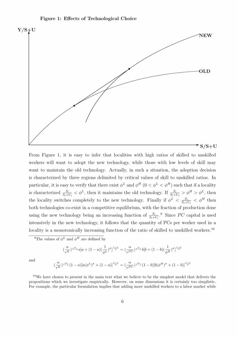
Figure 1: Effects of Technological Choice

6Y/S+U

-S/S+U

OLD

NEW

´´´´´´´´´´´´´́

s

s

From Figure 1, it is easy to infer that localities with high ratios of skilled to unskilled

workers will want to adopt the new technology, while those with low levels of skill may

want to maintain the old technology. Actually, in such a situation, the adoption decision

is characterized by three regions delimited by critical values of skill to unskilled ratios. In

particular, it is easy to verify that there exist φL and φH (0 < φL < φH) such that if a locality

is characterized SiSi+Ui

< φL, then it maintains the old technology. If SiSi+Ui

> φH > φL, then

the locality switches completely to the new technology. Finally if φL < SiSi+Ui

< φH then

both technologies co-exist in a competitive equilibrium, with the fraction of production done

using the new technology being an increasing function of SiSi+Ui

.9 Since PC capital is used

intensively in the new technology, it follows that the quantity of PCs per worker used in a

locality is a monotonically increasing function of the ratio of skilled to unskilled workers.10

9The values of φL and φH are defined by

(α

rK)

α1−α a[a+ (1− a)(

1

φL)σ]

1−σσ = (

α

rPC)

α1−α b[b+ (1− b)(

1

φH)σ]

1−σσ

and(α

rK)

α1−α (1− a)[a(φL)σ + (1− a)]

1−σσ = (

α

rPC)

α1−α (1− b)[b(φH)σ + (1− b)]

1−σσ

10We have chosen to present in the main text what we believe to be the simplest model that delivers thepropositions which we investigate empirically. However, on some dimensions it is certainly too simplistic.For example, the particular formulation implies that adding more unskilled workers to a labor market while

6

This forms the basis of Proposition 1.

Proposition 1: After the arrival of a PC-based, skilled-biased technology, the ratio of PCs

per worker will be an increasing function of a locality’s ratio of skilled to unskilled workers.

Proposition 1 indicates that skill biased technologies are adopted most aggressively by lo-

calities in which skill is relatively abundant, and therefore the observable aspects of the

technology – such as here PC capital — are most prevalent in localities with more skill.

This implication is the focus of the Doms & Lewis (2006) paper. Here, we want to go further

and derive a set of additional implications in order to examine more closely the relevance of

a biased technology adoption model for understanding differences in outcomes across locali-

ties. To this end, we first extend slightly Proposition 1 and derive a corollary that captures

the incentive mechanism that lead to the different adoption decisions. Note that from an

individual firm’s perspective, the differential adoption decisions across localities must reflect

different incentives induced by factor prices. In effect, in localities with initially high ratios

of skilled to unskilled labor, the relative price of skilled labor is initially low (prior to the

availability of the new technology), favoring the adoption of a technology which uses skill

intensively. This implication is expressed in Corollary 1.

Corollary 1: The ratio of PCs per worker is an increasing function of a locality’s initial

ratio of skilled to unskilled wages.

Proposition 1 and Corollary 1 focus on the effects of local market condition on adoption

decisions. We now want to change perspective and examine instead how the arrival of the

new technology affects relative wages. In particular, we first want to emphasize how changes

in the return to skill, as expressed by the change in the (log) ratiowSiwUi, vary across localities

faced with similar new options. This is captured in Proposition 2 and Corollary 2.

keeping the number of skill workers constant would lead to a decrease in the number of PCs. This implicationis likely false as it results from the assumption that there is no possibility of using PCs in the traditionaltechnology. A slightly generalized formulation, which reverses this implication, is one where the traditionaltechnology use both structures and equipment. At t = 0, the PC becomes available. The PC can thenbe used either as a substitute for equipment in the traditional technology, or it can be used in a new formof organization which is both skill-biased and uses PC more intensely than the traditional technology (isthe sense that, as given factor prices, it uses a greater number of PC per worker). This later form ofwork organization is what we envision as the new technology. It can be easily verified that this alternativeformulation is consistent which the all the propositions presented in the paper, but it does not imply thatthe number of PCs used would decrease with an increase in unskilled labor.

7

Proposition 2: The arrival of the skilled biased technology causes the returns to skill to

increase most in localities where skill is abundant.

The content of Proposition 2 can be obtained by deriving the relationship between the

return to skill and the supply of skill before and after the arrival of the new technology, and

taking the difference between the two. This relationship is expressed analytically below and

graphically in Figure 2. As can be seen, for localities with very low initial supply of skilled

workers, relative wages don’t change since the new technology is not adopted. For localities,

with φH < SiSi+Ui

, they experience the largest increase in the returns to skill since they switch

entirely to the new technology which acts as an increase in the demand for skill. Finally, for

localities in partial adoption region φL < SiSi+Ui

< φH , the increase in the returns to skill in

strictly increasing in the supply of skill since the endogenously induced demand for skill is

increasing with skill.

∆ lnwsi

wUi

= 0 ifSi

Si + Ui

≤ φL

∆ lnwsi

wUi

= (1− σ)[logSi

Ui

− log φL] if φL <Si

Si + Ui

≤ φH

∆ lnwsi

wUi

= (1− σ)[log φH − log φL] if φH <Si

Si + Ui

Proposition 2 expresses how the arrival of the new technology induces a positive association

between the supply of skill and changes in returns to skills. However, the proposition by-

passes the channel through which this arises and, in this sense, it represents a reduced form

relationship. Corollary 2 addresses this issue by combining Propositions 1 and 2 to highlight

how it is the adoption of the PC-intensive technology that leads to increases in returns to

skill.

Corollary 2: Returns to skill increase most in localities which choose to use PCs most

intensively.

Any approach taken to evaluate Corollary 2 must acknowledge the endogeneity between

PCs and returns to skill. Corollary 2 implies that its is the adoption of PCs induced by

differences in initial supply of skill (or initial returns to skill) that causes increases in returns

to skill. Viewed in this light, Corollary 2 can be evaluated by employing an IV strategy where

8

either initial (pre-PC-adoption) levels of skill or returns to skill are used as instruments for

PC-adoption in a regression of changes in the returns to skill on PC-adoption.

6∆ wc

wH

Figure 2: Effect of Initial Supply on Change in Relative Wage

-S/U

´´´´´´´´´´´´´´´´´́

At first pass, Proposition 2 may possibly appear to contradict the law of supply and demand

because it predicts an increase in return to skill where supply is most abundant. However,

this is not the case since the model does not allow the level of the return to skill to be

positively related to supply. In fact, as stated in Proposition 3, even after the introduction

of the skill-biased technology, the returns to skill must remain a weakly decreasing function

of the supply of skill. Note that it is possible for the arrival of the skill biased technology

to cause the disappearance of a negative relation between return and supply if localities are

concentrated in the technology-mixing zone (φL < SiSi+Ui

< φH), since in this region there

is factor price equalization. However, in the absence of any externalities in adoption, the

model implies that the relationship between returns to skill and supply of skill cannot be

positive even after the introduction of the skilled-biased technology.

9

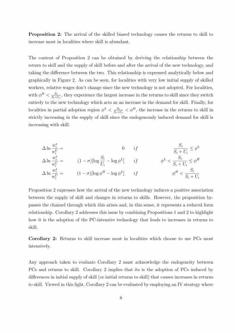
Proposition 3: The arrival of the skill biased technology cannot induce a positive associa-

tion between the return to skill and the supply of skill.

The content of Propositions 2 and 3 can be easily inferred from Figure 1. Because the returns

to skill in this figure are captured by the slope of the production function, we can note that

the slope of the outer envelop is weakly decreasing in the fraction of skilled workers. This

is the content of Proposition 3. In contrast, if we consider the change in the return to skill

induced by the new technology for an initial supply in the region (φL < SiSi+Ui

< φH), we see

that the increase in the slope is larger for initial higher levels of supply. The reason is that

the return to skill was initially more depressed in the higher supply localities and therefore

the new technology allows for greater induced demand for skill in such areas. The content

of Proposition 3 is depicted in Figure 3. In this figure we see that the availability of the new

technology alters the relationship between returns to skill and supply. However, the slope of

the new relationship is nowhere positive. Note that in the region φL < SiSi+Ui

< φH , the slope

of the relationship is zero. This arises since the technological choice allows the reallocation

of additional skill between the two technologies without affecting the returns.11

Now that we have examined the effects of supply on both adoption and wage change, we can

therefore combine the two to obtain Corollary 3.

Corollary 3: The return to skill will not be larger in localities with more intensive use of

PCs.

Corollary 3 indicates that although PC adoption and increases in the returns to skill should

go hand-in-hand (as stated in Corollary 2), such positive co-movement cannot induce an

outcome where the returns to skill are higher in a locality with a higher PC-intensity. The

reason for this result comes directly from the fact that PC adoption is endogenous in the

framework. To be more precise, PCs are adopted more aggressively in one locality versus

another only because the cost of skill is lower. Therefore, PC capital cannot be more intensely

used in a locality with a higher cost of skill. By contrast, if the adoption and subsequent

use of PCs were viewed as an exogenous phenomena (as is the case in many papers), then

it would be natural to expect to find a positive association with PC use and returns to skill

(assuming that PCs are a skill-biased technology). Hence, this prediction nicely illustrates

how a model of endogenous technology adoption differs from more conventional models with

11This mechanism is identical to that underlying factor price equalization zones in international tradetheory.

10

exogenous technological change.12

6wc

wH

Figure 3: Effect of Supply on Relative Prices

-S/L

PPPPPPPPPPPPPPPPPPPPPPPPPPPRE

PPPPP XXXXXXPOST

So far we have focused on the implications of the process of technology adoption on the

returns to skill, but we have not examined implications for each component, that is, impli-

cations for changes in the the wage of skilled workers and wages of unskilled workers taken

individually. Proposition 4 addresses this point.

Proposition 4: After the arrival of the skill biased technology, the wage paid to skilled

workers should increasemost in localities which adopt PCs most intensively, or alternatively

in localities with either an initially low return to skill or a high supply of skill. Conversely,

the wage paid to unskilled workers should decrease most in localities which adopt PCs most

12The implication of endogenous adoption stated in the previous propositions and corollaries would bemodified if the adoption process involved externalities. For example, suppose there existed a network typeexternality associated with the adoption of the new technology, that is, suppose that as more local productionwas done with the new technology, the productive performance of the new technology increased. In sucha case, it would be possible to have returns to skill being positively correlated to PC-intensity. Also, thereturns to skill could be, at least over a range, an increasing function of the supply of skill.

11

intensively, or alternatively in localities with either an initially low return to skill or a high

supply of skill.

Proposition 4 indicates that the model of endogenous technology adoption predicts opposite

responses for high skilled wages versus low skilled wages to local supply conditions. In

particular, as in the case of Proposition 2, Proposition 4 predicts positive relationships

between changes in wages for a skill group and its relative supply. The intuition is again

simple. If a locality has an abundance of skilled workers, then it should adopt the new

technology aggressively which induces an increased demand for skill and a substitution away

from less skilled workers. If instead the locality has mostly unskilled workers, then it does

not adopt the new technology intensely and hence such a locality should not experience

a strong reduction in the demand for less skilled workers. As discussed in Section 5, the

prediction that the adoption of PCs leads to a decrease in the wage of less skilled workers is

a feature that will help differentiate the current model from alternative explanations.

So far we have emphasized the role of differences in skill mix at the city level on technology

adoption and on the subsequent changes in wages. However, we have not offered any expla-

nation for the observed difference in skill mix across cities (which are stark and are shown in

the next section), we have simply noted that it predates the arrival of the PC and therefore

may plausibly be taken as exogenous to the process of PC adoption. One possible reason for

differences in skill mix across cities is the presence of amenities that act as luxury goods. As

discussed in Black, Kolesnikova and Taylor (2004), such amenities can help explain differ-

ences in skill mix, differences in returns to skill and differences in housing prices across cities.

In fact, the data patterns presented in this section can be shown to be consistent with an

environment where (1) skilled workers are mobile across cities and land prices adjust to make

such individuals indifferent between locations (as discussed in Black, Kolesnikova and Taylor

(2004)), and (2) cities gained the option of adopting a PC and skill-intensive technology over

the period 1980-2000.13 However, for simplicity we have not pursued this avenue here.

13Another possible reason for differences in skill levels across cities are differences in industry composition.However, as shown in Doms and Lewis (2006), industry composition accounts for very little of the cross-sectional variation in skill levels.

12

3 Data

Section 2 highlighted several implications of viewing technological adoption as driven by

principles of comparative advantage. Our goal now is to examine whether city-level outcomes

observed over the 1980-2000 period exhibit the patterns implied by such a model. We choose

to focus on this period for several reasons. First, this is a period often referred to as one

of technological revolution due to astounding technical progress and diffusion of information

technology. Hence it is a perfect candidate period to see whether our neoclassical model

of technological adoption is relevant. Second, it is a period in which returns to education

have increased substantially, for which skill-biased technological change is a primary suspect.

Therefore, it is particularly relevant to examine whether this period is best characterized as

reflecting the effects of exogenous technological change (in line with much of the literature

which treats the extent and bias of technological change as an exogenous driving force) or

whether instead it reflects a process of endogenous choice of production techniques.14

The city-level data we use can roughly be divided into two categories; technology and demo-

graphic. The technology data is derived from establishment-level information on technology

use and is described in more detail in Doms and Lewis (2006). About 160,000 establishment-

level observations per year are used to compute the PC intensity (PCs per employee) of each

city in our sample (230 cities).15 Our PC intensity measure is an industry-adjusted measure;

in computing the PC intensity, we control for the 3-digit SIC industry interacted with 8

establishment size classes, for a total of over 1,800 interactions.16

We focus on PCs instead of other IT technologies for several reasons. First and foremost,

businesses spent about 90 percent more money on PCs during the 1990s than on other types

14Note that it could be possible that the extent of bias of technical change is endogenous at the nationallevel, but not at the city level since markets across cities are well integrated. In such a case, our approachof focusing on city level outcomes would not identify elements of endogenous technological change. In otherwords, our empirical work evaluates the joint hypothesis that technological adoption is a phenomena thatreacts to market conditions and that the labor markets in cities across the US are not perfectly integrated.

15To increase the precision of our city-level measures, the 1990 PC intensity measure uses data from1990 and 1992 and the 2000 PC intensity measure relies on 2000 and 2002 data. Doms and Lewis (2006)define “city” primarily as consolidated metropolitan statistical areas (CMSAs). The logic was to derive citydefinitions that corresponded to the idea of a local labor markets. In some cases, CMSAs were modified tomore closely capture the concept of a labor market. Our results throughout the paper are insensitive to howwe define labor markets in especially large, contiguous areas, such as in and around New York City.

16The SIC-size interaction allows for the possibility that, for instance, large banks perform different oper-ations than small banks. As described in Doms and Lewis (2006), our city-level measures of PC intensityare strongly correlated with other measures that control for 4-digit SIC and for measures that also controlfor the firm to which an establishment belongs.

13

of computers. Also, spending on PCs is likely correlated with other information technology

spending, such as spending on software, computer networking equipment, printers, et cetera.

Finally, we were able to obtain consistent measures of PCs over this period.17

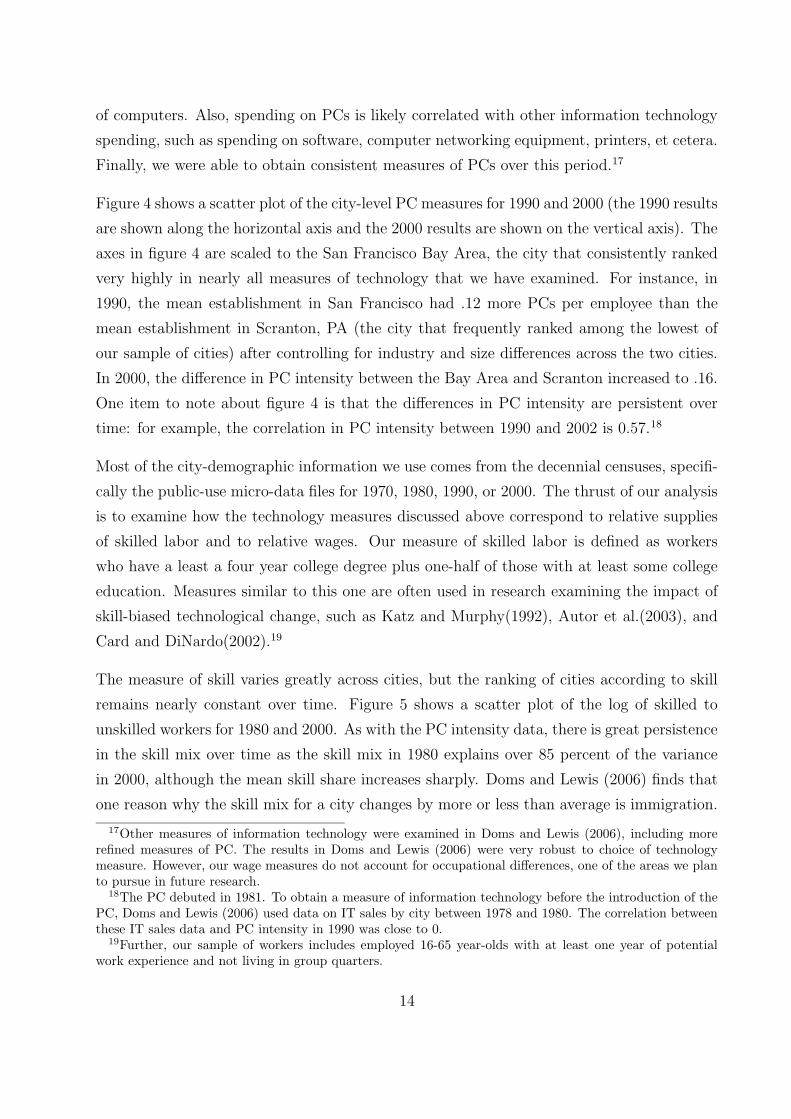
Figure 4 shows a scatter plot of the city-level PC measures for 1990 and 2000 (the 1990 results

are shown along the horizontal axis and the 2000 results are shown on the vertical axis). The

axes in figure 4 are scaled to the San Francisco Bay Area, the city that consistently ranked

very highly in nearly all measures of technology that we have examined. For instance, in

1990, the mean establishment in San Francisco had .12 more PCs per employee than the

mean establishment in Scranton, PA (the city that frequently ranked among the lowest of

our sample of cities) after controlling for industry and size differences across the two cities.

In 2000, the difference in PC intensity between the Bay Area and Scranton increased to .16.

One item to note about figure 4 is that the differences in PC intensity are persistent over

time: for example, the correlation in PC intensity between 1990 and 2002 is 0.57.18

Most of the city-demographic information we use comes from the decennial censuses, specifi-

cally the public-use micro-data files for 1970, 1980, 1990, or 2000. The thrust of our analysis

is to examine how the technology measures discussed above correspond to relative supplies

of skilled labor and to relative wages. Our measure of skilled labor is defined as workers

who have a least a four year college degree plus one-half of those with at least some college

education. Measures similar to this one are often used in research examining the impact of

skill-biased technological change, such as Katz and Murphy(1992), Autor et al.(2003), and

Card and DiNardo(2002).19

The measure of skill varies greatly across cities, but the ranking of cities according to skill

remains nearly constant over time. Figure 5 shows a scatter plot of the log of skilled to

unskilled workers for 1980 and 2000. As with the PC intensity data, there is great persistence

in the skill mix over time as the skill mix in 1980 explains over 85 percent of the variance

in 2000, although the mean skill share increases sharply. Doms and Lewis (2006) finds that

one reason why the skill mix for a city changes by more or less than average is immigration.

17Other measures of information technology were examined in Doms and Lewis (2006), including morerefined measures of PC. The results in Doms and Lewis (2006) were very robust to choice of technologymeasure. However, our wage measures do not account for occupational differences, one of the areas we planto pursue in future research.

18The PC debuted in 1981. To obtain a measure of information technology before the introduction of thePC, Doms and Lewis (2006) used data on IT sales by city between 1978 and 1980. The correlation betweenthese IT sales data and PC intensity in 1990 was close to 0.

19Further, our sample of workers includes employed 16-65 year-olds with at least one year of potentialwork experience and not living in group quarters.

14

Cities such as Fresno, Stockton, and El Paso received relatively large numbers of unskilled

immigrants over the past several decades, resulting in lower than average skill appreciation.

Our measure of relative wages is computed using the wages of people who report exactly a

high-school degree or GED and people with exactly a four years of post high school education.

We adjusted wages for each group by controlling for a fourth-degree polynomial in potential

work experience, a female dummy, an immigrant dummy, and a dummy for people born after

1950. Although the results presented in subsequent tables use these adjusted relative wages,

the results are robust to using non-adjusted wages as well.

We also construct several city-level measures that we label as city controls. These measures

include the log of the size of the labor force and percent of the workforce in a city are African

American, female, Hispanic, and U.S. citizens. Additionally, we construct 9 industry controls

which reflect the employment distribution across major industry groups within each city.

In the empirical work that follows, it is necessary for us to use instruments that are correlated

with the human capital in a city but not correlated with any of the unobserved determinants

of technology adoption. Instruments used in Doms and Lewis (2006) relied on the historical

density of colleges in an area. There are three reasons why the presence of colleges in an area

may increase the general skill level of that area. The first is that the presence of colleges

in an area reduces the cost of obtaining higher education for an area’s residents. Second,

college graduates may more likely settle in areas where they went to school as a result of low

search costs. Finally, areas that have an abundance of colleges may also have amenities that

college graduates place relatively high values on.20 One instrument we use, following Moretti

(2004), is a dummy for whether or not the metropolitan area has a land-grant college. Land-

grant colleges came into existence after Congress in 1862 passed the Morrill Act, which gave

states land to fund the creation of university-level agricultural schools. Doms and Lewis

(2006) shows that areas with land-grant colleges tend to have a significantly higher college-

educated share. In addition to the information on land-grant colleges, we also use lagged

information on local college density generally. There has been a dramatic growth in two-

year colleges since World War II (documented in Kane and Rouse, 1999) which may have

raised educational attainment in areas which received new schools. To capture the effect

non-land-grant may have on the local college share, we construct additional instruments

20As a result, human capital theory predicts otherwise similar individuals will have higher college at-tainment (Card, 1999). At an individual level, for example, several studies have showed that the distancea person lives from a college when they are growing up predicts their college attainment (e.g. Kane andRouse, 1995; Card, 1995).

15

using information on enrollment at two- and four-year colleges in 1971 in each metropolitan

area.21

4 Empirical results

Our presentation of empirical results closely follows the order of the Propositions and Corol-

laries presented in Section 2. We begin by examining the determinants of technology adoption

as measured by diffusion of PCs (Proposition 1). The first results echo those presented in

Doms and Lewis (2006). We then go further by examining whether returns to skill in 1980,

at the beginning of the diffusion process for PCs, are negatively associated with the intensity

of PC use in 2000 (Corollary 1). We next turn to examining implications of the model for

changes in the returns to skill, as measured by the ratio of college wages to high school

wages. In particular, we explore whether the data exhibits a positive co-movement between

PC-adoption and changes in the returns to skill as implied by Corollary 2, but do not reveal

a positive association between the level of returns to skill and PC use as implied by Corollary

3. We also report the reduced form implications of the model regarding the changes in the

returns to skill and the supply of skill (Proposition 2), in addition to examining changes in

the relationship between the level of return and the supply of skill (Proposition 3). Finally,

we examine the relationship between PC-adoption and changes in the wages paid to high

school workers and college workers separately (Proposition 4).

4.1 PC adoption and local market conditions

To begin and to illustrate the strength of the relationship between PC adoption and skills,

Figure 6 shows a scatter plot of PC intensity against the log ratio of skilled versus unskilled

labor for 2000. To examine the relationship between these variables more rigorously, Table 1

reports a series of regression results. The first column of Table 1 reports the results obtained

by regressing our city-level measure of PCs-per-worker on the log ratio of college to high

school equivalent workers. As can be seen from the table, cities with a high fraction of

college educated workers in 2000 also had adopted PCs more intensively by the year 2000.

21Doms and Lewis (2006) also examine instruments based on immigration patterns for the change in collegeshare. Doms and Lewis (2006) find very similar results in PC adoption equations between the college-basedinstruments for the level of human capital and the immigrant-based instruments for the change in humancapital.

16

The data in Figure 6 demonstrate that the relationship is not driven by outliers. Since cities

that use information technology more intensively may attract higher educated workers, this

observation does not imply that the local supply of college educated workers caused a greater

adoption of PCs. In order to address the possibility of reverse causation, Column 4 reports

an estimate obtained by instrumental variables, where the instruments, which are described

more fully in the previous section, correspond to measures of local college accessibility and

attendance as of 1971, which is well before the availably of PCs.22 The IV estimate is almost

identical to the OLS estimate, suggesting that the endogeneity of worker migration cross

cities to take advantage of more IT intensive cities may not be very strong.

Columns 2,3,5 and 6 follow up on this conjecture by breaking down the local skill measure

into its level in 1980 (just before the introduction of the IBM PC) and its change between

1980 and 2000. The only difference between columns 2 and 3, and between columns 5 and 6,

is the addition of a set of city level controls.23 The estimates in columns 2 and 3 are obtained

by OLS, while those in column 5 and 6 are obtained by IV. The results reported in Column 5

and 6 are based on the same 1971 variables to instrument both the the level and the change

in skill supply. Note that if the supply of skills is exogenous to the process of technology

adoption, then the coefficients on both the 1980 level of skill and the change in skill between

1980 and 2000 should have the same size coefficient, and this is what is observed in all but

one case.24 Furthermore, the estimates obtained by OLS and IV are very similar adding

support to the notion that it is the local supply of skill that favored differential adoption

patterns across US cities and not the reverse.25 While there are many models or mechanisms

of technological change that could potentially explain the observations presented in Table 1,

our goal now is to examine whether the mechanism outlined in the theory section is relevant

by examining implications for wages.

The estimates presented in Table 1 indicate that cities with a more educated labor force

as of 1980 adopted PCs more aggressively between 1980 and 2000. The neoclassical model

presented in Section 2 suggests that such an outcome arises due to the price incentive by

firms in cities with initially expensive low skilled workers (relative to high skilled workers)

to adopt skill-biased technologies.26 In Table 2 we examine whether the data support such a

22The first stage had an r2 of .32.23The city level controls correspond the size of the labor force, unemployment rate, the fraction of popu-

lation which is female, percent African-American, and U.S. citizens.24We tested the equality of these coefficients, and the p-values are reported on the last row of the table.25Recall that the measure of city-level PC-use we use controls for a cities industrial composition.26A clear negative trend between relative wages and the supply of skilled labor for 1970, 1980 and 1990 is

17

mechanism by regressing PC intensity in 2000 on the relative cost of skilled versus unskilled

labor in 1980. As can be seen in Column 1, cities with low relative cost of skills in 1980 are

observed to be using PCs more intensively as of 2000. In the second column, we add the

change in the ratio of college and high-school educated workers, and in column 3 we also

control for share of employment at the industry level (in two digit industries). In the fourth

column, we instrument the change in the ratio of college to high school educated workers,

again using 1971 college attainment and access variables as instruments. In all cases, we

find that the return to skill as of 1980 has a significant negative effect on subsequent PC-

adoption. We also find that after controlling for initial returns to skill, an increase in the

college population favors more PC-adoption. Once again we find only minor differences

between treating changes in the college population as exogenous to the adoption process as

compared with estimating by IV, further suggesting that the endogeneity of skill supply to

PC-adoption process is likely minor.

4.2 Returns to skill and PC adoption

We now turn to the relationship between the adoption of PCs and changes in the returns

to skill. Recall that our model implies a positive association between these two endogenous

variables. In Table 3 we report results obtained by regressing the change in the return to

skill over the period 1980-2000 on the extent of PC-adoption in 2000. In the first 3 columns

we estimate the relationship by OLS, which likely provides a downward biased estimate due

to the endogeneity of PC-use. In particular, given our theoretical framework, we expect

that unobserved variables which lead to higher returns to skill would result in lower PC

adoption. As can be seen, our OLS results find a positive, but weak and insignificant

relationship between these two variables. In columns 4 to 6, we report IV estimates where

we instrument the PC-adoption variable by the 1980 ratio of college educated workers to

high school educated workers. As shown in Table 1, the first stage of this regression works

well. The IV results indicate a strong positive association between PC-adoption and changes

in returns to skill, even after including city and industry controls. We also estimated (but

did not report here) the relationship using as an instrument the 1980 value of the returns

to skill (as suggested by Table 2). In this case, we also found a very significant and robust

positive relationship between changes in returns to skill and PC-adoption. The estimates

shown by the scatter-plots in figures 8a-8c.

18

are bigger than the ones reported in Columns 4-6, but are less precise.27

In addition to predicting that localities that adopt PCs intensively should witness greater

increases in returns to skill, the model also predicts that the adoption process should not lead

to a situation where returns to skill are higher in cities that adopted PCs most intensively. To

examine this implication of the model, Table 4 reports estimates of the relationship between

returns to skill in 2000 and the use of PCs in 2000. The first 3 columns report results based

on estimating the relationship by OLS, and in the last three columns the relationship is

estimated by IV, where the ratio of college to high school equivalent workers in 1980 is the

instrument. In none of these cases do we observe a positive relationship between PC-use

and returns to skill; in some cases we actually find a significant negative relationship. Taken

together, the results in Tables 3 and 4 provide considerable support for the view that PC-

adoption and changes in returns to skill should be viewed as jointly determined, and that

the process appears to conform to the neoclassical principles outlined in Section 2.

4.3 Reduced form relationship between returns and skill supply

Tables 3 and 4 report results associated with examining the implications of the model as

stated in Corollaries 2 and 4. For completeness, it is also of interest to directly examine

the reduced form relationship emphasized by Proposition 2 and 3. To this end, we begin

by showing a plot, Figure 7a, of the changes in the returns to skill and the initial supply of

skill. As can be seen, there is a clear positive relationship with a regression slope coefficient

of .07 and standard error of .01. Figures 7b and 7c decompose the changes by decade and

show that the change in relative wages between 1980 and 1990 had no significant relationship

vis-a-vis skill share, whereas the change in 1990-2000 had the most pronounced relationship

with skill share.28 This suggests that PC adoption may have been a much more important

force in explaining changes in wage differentials movements in the 1990s then during the

introductory phase of the 1980. Turning to a fuller set of regressions, the first three columns

of Table 5 report the results of regressing change in the returns to skill over the period 1980

to 2000 on the 1980 ratio of college to high school educated workers and the change in skill

27As a robustness check, we ran the regressions in Table 3 separately for the change in relative wages ofmen only and women only. The results for each group were similar to those reported in Table 3 althoughthe results for women were, on average, a bit stronger than those for men.

28As we have mentioned previously, the PC was introduced in 1981, and hence we frequently begin ouranalyses with data in 1980. However, it was not until the 1990s that information technology became asignificant share of the capital stock and a significant contributor to GDP growth.

19

supply over the period 1980-2000.

In order to better interpret the coefficients on the initial supply of skill and the coefficient

on the change in the supply of skill, it is helpful to recall that the theory implies that the

arrival of a skilled biased technology will cause a flattening of the relationship between the

returns to skill and the local supply of skill (as depicted in Figure 3). If we approximate this

prediction by a change in the linear relationship between return and relative supply, then we

can see that theory predicts the change in the returns to skill to be positively related to the

initial level of skill and negatively related to the change in skill. In order to see this more

clearly, let us express the initial relationship between return and supply by:

wSi,0

wUi,0

= α1 + α2Si,0

Ui,0

and denote the relationship after the arrival of the technological option by:

wSi,1

wUi,1

= β1 + β2Si,1

Ui,1

where α2 < β2 ≤ 0.

Then the change in the returns to skill is then given by

∆wSi

wUi

= (β1 − α1) + (β2 − α2)Si,0

Ui,0

+ β2∆Si

Ui

with β2 − α2 > 0 and β2 ≤ 0. In words, the coefficient on the initial supply should capture

the change in the slope of the relationship between return and relative supply of skill–which

the theory predicts in positive – and the coefficient on the change in supply should capture

the final slope– which according to the theory could be either negative or zero in the absence

of externalities.

Interestingly, the results in Columns 1-3 of Table 5 indicate a positive relationship between

the change in returns and the initial supply of skill, while simultaneously observing a negative

or zero relationship between the change in returns and the supply of skill. In fact, the latter

relationship is sufficiently weak to suggest it may be a zero relationship. The last three

columns examine the effect of replacing the initial skill ratio with the initial value of the

20

returns to skill, as also suggested by Proposition 2. Here we see, consistent with the theory,

that returns to skills increased most in cities where the returns were initially low.

The results presented in Table 5 were aimed at evaluating the implications of Proposition

2. The goal of Figure 8 and Table 6 is to examine more directly the local flattening of

the relationship between returns to skill and supply of skill implied by the theory. To this

end, Figure 8 plots the relative wages and the supply of skill for 1970, 1980, 1990 and 2000

and Table 5 reports the associated regression estimates. From the figures and the table

we can see that the slope of the relationship between returns to skill and the supply of

skill is significantly negative in 1970, 1980 and 1990.29 By contrast, in 2000 the returns

to skill/supply of skill relationship essentially evaporates at the local level. This finding is

consistent with Proposition 3 if cities are finding it optimal to simultaneously use both old

and new technologies. Note that these observation are also consistent with those presented

in Table 5, which can be viewed as providing first difference estimates of both the slope in

2000 (through the coefficient on the change in supply of skill) and the change in the slope

between 1980 and 2000.30

4.4 Changes in wages and PC adoption

In order to complete our exploration of the implications derived in Section 2, namely Propo-

sition 4, Table 7 displays results of changes in college and high school real wages separately.

In this table we see that the growth in wages of high school educated workers (in columns

1,3 and 5) was negatively associated with the extent of PC adoption within cities, and this

pattern is observed whether the relationship is estimated by OLS or by IV using the city

level market conditions in 1980 as instruments for PC adoption. Note that this result is not

implied by the previous results since high school educated workers could have made wage

gains in cities that adopted PCs aggressively while allowing college educated workers to do

even better. However, this is not what is observed. Instead, consistent with the theory, we

29Because of data issues, we could only focus only on 140 of our 230 sample of our cities for 1970.30An alternative explanation for such convergence is that the supplies of skills converges across cities.

However, there was actually only minimal convergence in the fraction of college equivalent workers acrosscities over this period, with the variance of the fraction college equivalents per city being almost the samein 2000 as in 1980. This contrasts with Glaser (2005) which reports a divergence in the concentration ofcollege educated over this period. His result relies on looking precisely at the fraction of workers with 4years of college or more. If instead we look at the fraction of college equivalents, where workers with postsecondary education are allocated equally between high skill and low skill, then there is no indication ofeither convergence or divergence. Finally, if we look at the log of the ratio of college equivalents to highschool equivalents, there is evidence of convergence but the coefficient is nowhere near -1.

21

see that high school educated workers were negatively affected by the adoption of PC in an

absolute sense, not just a relative sense.

For college educated workers, the OLS results do not uncover much of a relationship between

their wage change and the adoption of PCs. However, since both variables are endogenous,

the coefficient can be expected to be biased. Accordingly, we also report results where

we instrument the extent of PC-adoption by the ratio of college and high school educated

workers in 1980 and the return to college in 1980 (using only one of these instruments gives

similar, but slightly less precise, estimates). The IV results indicate that college educated

workers had faster wage gains in cities that adopted PCs most intensely, nearly to the same

extent that high school workers lost.31

5 Alternative explanations

The evidence presented in Tables 1 to 8 provide considerable support for the model of endoge-

nous technology adoption we presented in Section 2. However, such evidence does not imply

that this model is correct since the data may be consistent with alternative interpretations.

In this section we compare the properties of our model to several alternative technology

specifications used in the literature. We then examine two non-technological explanations

for our results; increased labor mobility and increased trade.

5.1 A comparison to other technology specifications

We ask whether the observed patterns can be easy explained by alternatives suggested by

the literature. One class of explanations we want to examine focuses upon the effects of a fall

in the price of equipment – such as PCs – within a stable production function framework.

To be more precise, let us continue to consider an environment with four factors of produc-

tion: traditional capital (K), PC/equipment (PC), skilled labor (S)and unskilled labor (U).

However, instead of considering two production functions, let us postulate a unique produc-

tion function denoted by f(Kt, PCt, St, Ut), with wages for skilled and unskilled labor given

by the marginal products. The issue we want to address is whether the cross-city patterns

31The result for college wages is robust to a wide variety of specifications, especially for specifications thatexamine the changes in wages in the 1990s. The results for high school wages are somewhat less robust, but,the high school wage results always imply a zero to negative relationship with PC adoption, a result in starkcontrast to that for college wages.

22

we have documented can be explained within this alternative framework as the result of a

common fall in the price of PC/equipment. If we impose no restrictions on the function f(·),

the answer to this question is a trivial yes since the stable production needs to be chosen

as the outer envelop of our two production function setup.32 Hence, to make this question

relevant, we need to ask whether the observed patterns could be explained by commonly

used parameterizations for such a function. To this end, we will focus on three nested CES

specifications.

The first parametrization we consider, denoted by f I , is in the spirit of the work by Katz

and Murphy (1992). In this case, the two types of capital form a sub-aggregate and the two

types of labor form a sub-aggregate. The function f I(·) can then be represented by

f I(Kt, PCt, St, Ut) = [Kσt + PCσ

t ]ασ [Sγ

t + Uγt ]

1−αγ

In the second case (F II), motivated by the capital skill-complementarity hypothesis, we allow

PC capital to be a complement to skilled labor. This case is represented by the following

production function

f II(Kt, PCt, St, Ut) = Kαt [[S

σt + PCσ

t ]γσ + U

γt ]

1−αγ σ < 0

The third possibility is motivated by Autor, Levy and Murnane (2003) which emphasizes

the substitution between PCs and unskilled workers. In this case, the production function

takes the form

f III(Kt, PCt, St, Ut) = Kαt [[Ut + PC]γ + S

γt ]

1−αγ

Given that we want to consider the situation where firms at the city level can rent both types

of capital on a common market, it is useful to define a reduced form production function

f̃ i, i = I, II, III, which represents the production possibility set at the city level, as follows

32Given that there is a fundamental observational equivalence between a choice of technique frameworkand a stable production function framework, one may ask what is the advantage of the choice of techniqueframework. One answer is that the endogenous choice of technique framework leads one to consider param-eterizations of the aggregate production function which otherwise would appear bizarre, un-intuitive andwould therefore likely be overlooked. By contrast, when such parameterizations are presented through thelens of the endogenous technological adoption framework, they become intuitive and credible contenders asexplanations to observations.

23

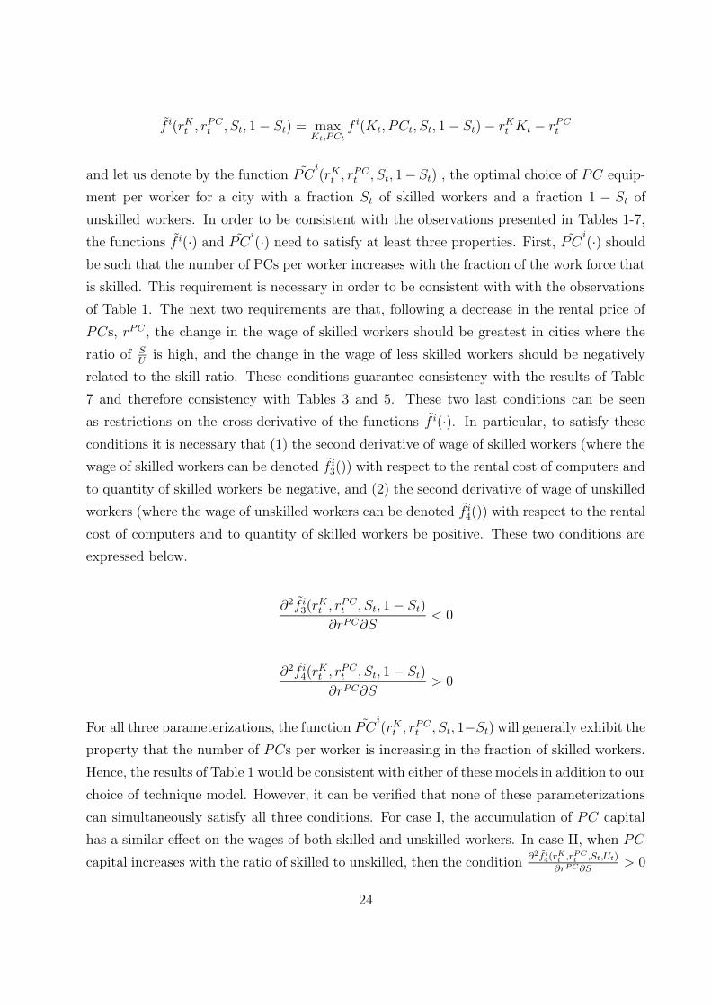
f̃ i(rKt , rPCt , St, 1− St) = max

Kt,PCtf i(Kt, PCt, St, 1− St)− rKt Kt − rPCt

and let us denote by the function P̃Ci(rKt , r

PCt , St, 1−St) , the optimal choice of PC equip-

ment per worker for a city with a fraction St of skilled workers and a fraction 1 − St of

unskilled workers. In order to be consistent with the observations presented in Tables 1-7,

the functions f̃ i(·) and P̃Ci(·) need to satisfy at least three properties. First, P̃C

i(·) should

be such that the number of PCs per worker increases with the fraction of the work force that

is skilled. This requirement is necessary in order to be consistent with with the observations

of Table 1. The next two requirements are that, following a decrease in the rental price of

PCs, rPC , the change in the wage of skilled workers should be greatest in cities where the

ratio of SUis high, and the change in the wage of less skilled workers should be negatively

related to the skill ratio. These conditions guarantee consistency with the results of Table

7 and therefore consistency with Tables 3 and 5. These two last conditions can be seen

as restrictions on the cross-derivative of the functions f̃ i(·). In particular, to satisfy these

conditions it is necessary that (1) the second derivative of wage of skilled workers (where the

wage of skilled workers can be denoted f̃ i3()) with respect to the rental cost of computers and

to quantity of skilled workers be negative, and (2) the second derivative of wage of unskilled

workers (where the wage of unskilled workers can be denoted f̃ i4()) with respect to the rental

cost of computers and to quantity of skilled workers be positive. These two conditions are

expressed below.

∂2f̃ i3(rKt , r

PCt , St, 1− St)

∂rPC∂S< 0

∂2f̃ i4(rKt , r

PCt , St, 1− St)

∂rPC∂S> 0

For all three parameterizations, the function P̃Ci(rKt , r

PCt , St, 1−St) will generally exhibit the

property that the number of PCs per worker is increasing in the fraction of skilled workers.

Hence, the results of Table 1 would be consistent with either of these models in addition to our

choice of technique model. However, it can be verified that none of these parameterizations

can simultaneously satisfy all three conditions. For case I, the accumulation of PC capital

has a similar effect on the wages of both skilled and unskilled workers. In case II, when PC

capital increases with the ratio of skilled to unskilled, then the condition∂2f̃ i4(rKt ,rPCt ,St,Ut)

∂rPC∂S> 0

24

will not be satisfied due to the fact that increases in PC capital leads to an increase in the

wage of less skilled workers. In case III, the change in relative wages due to a change in the

cost of PC is independent of of local factor supplies (as in case I), and accordingly can not

satisfy the conditions. Hence, these standard parametrizations of the aggregate production

function are not sufficiently flexible to offer an explanation of our set of observations, which

are easily explained with an endogenous technology model.

5.2 Labor mobility and trade

We now briefly examine the possibility that our cross-cities observations could be primarily

driven by some non-technological forces as opposed to the technological forces emphasized

by the model. In particular, we want to ask whether the observed patterns could be easily

explained by either an increase in labor mobility across cities or by increased goods market

integration (freer inter-city trade).

Let us start with labor mobility. One reason why there are less systematic differences in

returns to skill across cities in 2000 than in 1980 could be that labor mobility across cities

has increased; for instance, highly skilled individuals may have moved between cities where

skill is abundant to where it was relatively scarce. There are two problems associated with

this conjecture as an explanation to the observed patterns. First, it does not appear that

labor flows were in a direction that would favor convergence. For example, the correlation

between the change in college equivalent share by city over the period 1980-2000 with the

initial level of the college equivalent share in 1980 (or the return to skill in 1980) is very close

to zero.33 This is not surprising given that figure 5 showed very strong persistence in the

skill levels across cities from 1980 to 2000. Furthermore, if labor mobility were the dominant

force favoring a convergence in returns to skill across cities over this period – as opposed

to different speeds of technology adoption – we would not expect to observe the patterns

presented in Table 5. Recall that Table 5 showed that changes in the college-high school

wage differentials over 1980-2000 were positively and significantly related to the fraction of

college workers in 1980 and only weakly related to the change in the education composition

of the city.

A second mechanism that could remove systematic differences in returns to skill across cities

33Barry and Glaeser (2005) actually suggest that flows favored divergence. The difference with the resultreported here is they did not include any of the workers with post-secondary education in their measure ofskilled workers, while our college equivalent share measure includes a fraction of post-secondary workers.

25

is increased trade between cities. If the cost of trading between cities diminished significantly

over the period, this should favor a reallocation of industries to take advantage of differences

in skill supply across cities, thereby leading to factor price equalization. Taking this argument

to the next logical step then, it should also be the case that the local industry mix will become

more sensitive to the local factor endowments mix, as localities adapt industry mix to their

comparative advantage. We evaluate that possibility with the following statistic:

∑

j

CEj

Nj

[

∆

(

Nj,c

Nj

)

−∆

(

Nj

N

)]

whereCEjNjis the college equivalent share for industry j in 2000 and the term in brackets is

equal to the change in employment share in industry j and city c compared to industry j

in the nation as a whole between 1980 and 2000. This statistic tells us how much changes

in industry mix in c are expected to increase college share in c. If geographic integration

is occurring, then this statistic will be high for cities with a high college share, as college-

intensive industries disproportionately relocate to them, and low for cities with a low college

share.

In order to evaluate the extent to which this is the case, Figure 9 plots this statistic against

1980 college equivalent share (normalized to zero for the average city, i.e. the “excess”

college share). Note that this statistic is generally quite small - changes in industry mix

have virtually no differential impact on changes in college share in most cities - and there is

no sign that this relates positively to college share. For instance, one of the least educated

cities in our sample, Scranton, PA, has one of the larger increases in college-intensive industry

shares between 1980 and 2000. More generally, the coefficient from the regression line can be

interpreted as the proportion of differences in college share absorbed by changes in industry

mix: it is -.01 with a standard error of 0.01.34 Thus, at the level of industry detail available in

the censuses, there is no evidence that cities are “integrating” over time.35 This is consistent

with Lewis (2003) and Card and Lewis (2006) who find, using a similar approach, that

industry mix accounts for little of the skill mix differences across cities.

Another difficulty with the increased inter-city trade explanation is that, controlling for

34The regression used the same weights used in the regression presented in tables 1-7.35Industry mix is measured at the level of detail available in the 1980 PUMS, which is roughly equivalent

to the 3-digit SIC. We used the same mapping of Lewis (2003) to match the industry codes in the 1980 and2000 Censuses.

26

industry structure, there should be no systematic differences in PC-use across cities: cities

with more educated workers should have more skill and PC intensive industries but should

not use PCs more intensively within an industry. However, as documented in Table 1 and

illustrated in Figure 6, there is a strong positive link between PC use within industries and

the local supply of skill.

6 Conclusion

In this paper we began by highlighting the implications of a simple neoclassical model of

endogenous technology adoption. This model generates a number of predictions that we

test using a dataset on technology, skills, and wages for a set of 230 cities during the IT

revolution. We found the predictions of the model to conform well with the patterns found

in the data.

One important aspect of the model and the empirical results is that they tie together two

rather disparate strands of the literature. One strand has focused on how technological

change affects the demand for skilled labor while the other has examined how the supply of

skilled labor affects technological adoption. At the heart of the model is a choice facing firms

on which production technique to employ. In our model, we choose a parsimonious approach

and focus on just two choices. However, having these two choices produces a rich set of

implications (richer than can be generated from more standard nested CES specifications).

Our results are in many ways similar to those in the economic history literature, notably

Goldin and Sokoloff (1984). We find that cities that enjoyed relative abundance of skilled

labor in 1980 were those cities that adopted PCs (a skill-biased technology) most aggressively.

Further, cities that adopted PCs the most aggressively were also cities that witnessed the

largest increase in relative wages. In fact, the downward sloping relationship between relative

wages and the supply of skilled labor that existed in 1970, 1980, and 1990 had lessened

considerably by 2000. The increase in relative wages in response to PC adoption appears

to be driven by gains in wages of high-skilled workers and declines of wages of low-skilled

workers.

27

References

Acemoglu, Daron (1998), “Why Do New Technologies Complement Skills? Directed Tech-

nical Change and Wage Inequality,” Quarterly Journal of Economics, November 1998, vol

113, 1055-1089.

Acemoglu, Daron (2002), “Directed Technical Change”, Review of Economic Studies, volume

69. pp. 781-810.

Altonji, Joseph and David Card (1991), “Effects of Immigration on Labor-Market Outcomes

of Less-Skilled Natives,” in John Abowd and Richard Freeman, eds., Immigration, Trade,

and Labor p. 201-234.

Atkinson, Anthony B. and Joseph E.Stiglitz (1969), “A New View of Technological Change,”

Economic Journal, September, 79(3), pp.573-78.

Autor, David, Lawrence F. Katz and Melissa S. Kearney (2006), ”The Polarization of the

U.S. Labor Market,” mimeo.

Autor, David H., Frank Levy and Richard J. Murnane (2003), “The Skill Content of Recent

Technological Change: An Empirical Exploration,” Quarterly Journal of Economics, 118

(4): November 2003, p. 1279-1334.

Basu, Susanto and David Weil (1998), “Appropriate Technology and Growth,” Quarterly

Journal of Economics, November, 113(4), pp. 1025-54.

Beaudry, Paul and David Green (1998), “What is Driving US and Canadian Wages: Exoge-

nous Technical Change or Endogenous Choice of Technique?” (December), NBER working

paper 6853.

Beaudry, Paul and David Green (2003), “The Changing Structure of Wages in the US and

Germany: What explains the differences?” American Economic Review, June , pp 573-603.

Beaudry, Paul and David Green (2005), “Changes in U.S. Wages, 1976ndash2000: Ongoing

Skill Bias or Major Technological Change?” Journal of Labor Economics, vol 23 , pp. 609-

648.

Benhabib, Jess and Mark Spiegel (2005), ”Human Capital and Technology Diffusion,” forth-

coming, Handbook of Economic Growth, Philippe Aghion and Steven Durlauf, eds., North-

Holland, Amsterdam.

28

Black, Dan, N. Kolesnikova and L. Taylor (2004), “Understanding the Returns to Education

when Wages and Prices Vary by Location,” working paper.

Card, David (1995), “Using Geographic Variation in College Proximity to Estimate the

Return to Schooling,” in Louis N. Chiristofides, E. Kenneth Grant , and Robert Swidinsky,

Eds., Aspects of Labour Market Behaviour: Essays in Honour of John Vanderkamp. Toronto:

University of Toronto Press, p. 201-222.

Card, David (1999), “The Causal Effect of Education on Earnings,” Handbook of Labor

Economics. Volume 3A, 1999, p 1801-1863. Amsterdam, New York and Oxford: Elsevier

Science, North-Holland.

Card, David and John E. DiNardo (2002), “Skill-Biased Technological Change and Rising

Wage Inequality: Some Problems and Puzzles,” Journal of Labor Economics, 20 (4): October

2002, pp. 733-83.

Card, David and Ethan Lewis (2005), “The Diffusion of Mexican Immigrants During the

1990s: Explanations and Impacts,” NBER Working Paper no. 11552, August 2005.

Caselli, Francesco (1999), “Technological Revolutions,” American Economic Review, 89:1,

pp. 78-102.

Caselli, Francesco and W. John Coleman (2006), “The World Technology Frontier,” Ameri-

can Economic Review, forthcoming.

Comin, Diego and Bart Hobijn (2004), “Cross-Country Technology Adoption: Making the

Theories Face the Facts,” Journal of Monetary Economics, 2004, 51, 39-83.

Doms, Mark and Ethan Lewis (2006), “The Diffusion of Personal Computers Across the

U.S., 1990-2002,” Working Paper Series 2006-18, Federal Reserve Bank of San Francisco.

Gerschenkron, A. (1962), Economic Backwardness in Historical Perspective, Cambridge,

Belknap Press of Harvard University Press.

Glaeser, Edward (2005), “Urban Colossus: Why is New York America’s Largest City?,”

Harvard Institute of Economic Research Discussion Paper 2073.

Goldin, Claudia and Kenneth Sokoloff (1984), “The Relative Productivity Hypothesis of

Industrialization: The American Case, 1820 to 1850,” Quarterly Journal of Economics, 99

(August): 461- 488.

29

Habakkuk, H. J. American and British Technology in the Nineteenth Century. Cambridge:

Cambridge University Press, 1962.

Kane, Thomas J. and Cecilia Elena Rouse (1995), “Labor Market Returns to Two- and

Four-Year College,” American Economic Review 85(3): June 1985, p. 600-614.

Kane, Thomas J. and Cecilia Elena Rouse (1999), “The Community College: Educating

Students at the Margin Between College and Work,” Journal of Economic Perspectives

13(1): Winder 1999, p. 63-84.

Katz, Lawrence F. and Kevin M. Murphy, “Changes in Relative Wages, 1963-1987: Supply

and Demand Factors,” Quarterly Journal of Economics 112: 1992, p 291-303.

Krueger, Alan (1993), “How Computers Have Changed the Wage Structure: Evidence from

Microdata 1984-1989,” Quarterly Journal of Economics 108(1): 1993, p. 33-60.

Lewis, Ethan (2003),“Local, Open Economies Within the US: How Do Industries Respond to

Immigration?” Federal Reserve Bank of Philadelphia Working Paper no. 04-01, December

2003.

Lewis, Ethan (2005), “Immigration, Skill Mix, and the Choice of Technique,” Federal Reserve

Bank of Philadelphia Working Paper, May 2005.

Manuelli, Rodolfo and Ananth Seshadri (2004), “Frictionless Technology Diffusion: The Case

of Tractors,” working paper.

Moretti, Enrico (2004), “Estimating the Social Return to Higher Education: Evidence From

Longitudinal and Repeated Cross-Sectional Data,” Journal of Econometrics 121(1-2): July-

August 2004, p. 175-212.

Nervis, Allan (1962). The State Universities and Democracy. Urbana, IL: University of

Illinois Press, 1962.

Welch, Finis (2000), “Growth in Women’s Relative Wages and in Inequality Among Men:

One Phenomenon or Two?,” Papers and Proceedings of the American Economic Association,

pp. 444-449.

30

Table 1: PC Adoption and Education

OLS OLS OLS IV IV IV1 2 3 4 5 6

(

CH

)

20000.101 - - 0.102 - -( 0.009) ( 0.017)

(

CH

)

80- 0.100 0.084 - 0.097 0.094

( 0.009) ( 0.012) ( 0.017) ( 0.022)

∆(

CH

)

- 0.117 0.088 - 0.174 0.134( 0.022) ( 0.029) ( 0.050) ( 0.089)

City Controls - - yes - - yes

R2 0.34 0.34 0.58p-value - 0.65 0.02 - 2.38 0.32

The dependant variable is the number of PCs per worker at the city level corrected for industry

composition. The variable CHcorresponds to the log of the ratio of college equivalent workers to

high school equivalent workers. The instruments used are measures of local college availability

and attendance patterns as of 1971. The reported p-value is associated to the test of equality of

coefficients on(

CH

)

80and ∆

(

CH

)

, where the latter is the change over the period 1980-2000. The

city level controls correspond the the log of the labor force, the unemployment rate, the fraction of

city population which is female, African-American, and U.S. citizens. The regressions were run on

230 observations and weighted by the square root of the size of the labor force.

31

Table 2: PC Adoption and Initial Returns to Skill

OLS OLS OLS IV1 2 3 4

(

wC

wH

)

80-0.231 -0.250 -0.195 -0.201

( 0.054) (0.057) ( 0.059) ( 0.092)

∆(

CH

)

- 0.028 0.053 0.066( 0.028) ( 0.032) ( 0.138)

City Controls yes yes yes yes

Ind. Shares - - yes yes

R2 0.36 0.37 0.45

The dependant variable is the number of PCs per worker at the city level corrected for industry

composition. The variable(

wC

wH

)

80corresponds to the relative wage of college to high-school work-

ers. The instruments used are measures of local college availability and attendance patterns as

of 1971. The variable ∆(

CH

)

corresponds to the 1980-2000 change in the skill level of the city’s

workforce. The city level controls correspond the the log of the labor force, the unemployment rate,

the fraction of city population which is female, African-American, and U.S. citizens. The industry

controls include the share of the workforce in 12 major industry groups. The regressions were run

on 230 observations and weighted by the square root of the size of the labor force.

Table 3: Changes in Returns and PC Adoption

OLS OLS OLS IV IV IV1 2 3 4 5 6

(

PCL

)

20000.107 0.042 0.049 1.073 1.158 0.896

( 0.074 ) ( 0.077 ) ( 0.076 ) ( 0.259 ) ( 0.391 ) ( 0.293 )

∆(

CH

)

- - -0.061 - - -0.081( 0.035 ) ( 0.045)

City Controls yes yes yes yes yes yes

Ind. Shares - yes yes - yes yes

R2 0.26 0.35 0.36 - - -

The dependent variable is the change in the log ratio of college to high school wages, where wages

are adjusted for experience and gender. The instrument used for PCs is the ratio of college to high

school equivalent workers in 1980. See the notes in Table 1 and Table 2 about sample size, controls,

and weighting.

32

Table 4: Returns to Education and PCs in 2000

OLS OLS OLS IV IV IV1 2 3 4 5 6

(

PCL

)

2000-0.184 -0.234 -0.099 -0.526 -1.467 -3.398( 0.076) ( 0.078) ( 0.079) ( 0.217) ( 0.357) ( 3.433)

(

CH

)

2000- - -0.118 - - 0.229

(0.024) - ( 0.367)

City Controls yes yes yes yes yes yes

Ind. Shares - yes yes - yes yes

R2 0.39 0.46 0.52 - - -

The dependant variable is the log ratio of college to high-school wages, where the wages are adjusted

to control for experience and gender. The PC-measure controls for industry composition. See the

notes in Table 1 and Table 2 about sample size, controls, and weighting.

Table 5: Changes in Relative Wages and Skill: Reduced Form Relationships

1 2 3 4 5 6(

CH

)

19800.054 0.063 0.086 - - -

( 0.011 ) ( 0.014 ) ( 0.022 )

∆(

CH

)

-0.083 -0.040 0.001 -0.079 -0.047 0.013( 0.027 ) ( 0.034 ) ( 0.037 ) ( 0.027 ) ( 0.029 ) ( 0.032 )

(

wC

wH

)

1980- - - -0.320 -0.442 -0.474

( 0.062 ) ( 0.057 ) ( 0.059 )

City Controls - yes yes - yes yes

Ind. Shares - - yes - - yes

R2 0.16 0.35 0.41 0.17 0.44 0.51

The dependent variable is the change in log ratio of college to high school wages, where wages

are adjusted for experience and gender. See the notes in Table 1 and Table 2 about sample size,

controls, and weighting.

33

Table 6: Relative Wages and Supply of Skills (all OLS)

1(2000) 2(1990) 3(1980) 4(2000) 5(1990) 6(1980)(

CH

)

2000-0.001 - - -0.028 - -( 0.014 ) ( 0.015 )

(

CH

)

1990- -0.055 - - -0.055 -

( 0.012 ) ( 0.014 )(

CH

)

1980- - -0.066 - - -0.106

( 0.011 ) ( 0.012 )

C. Cont. - - - yes yes yes

R2 0.00 0.08 0.13 0.38 0.31 0.38

The dependent variable is log ratio of college to high school wages, where wages are adjusted for

experience and gender. The variable CHcorresponds to the log of the ratio of college equivalent

workers to high school equivalent workers. See the notes in Table 1 and Table 2 about sample size,

controls, and weighting.

Table 7: Changes in Wages and PCs: College and High School Educated Workers

1 2 3 4 5 6HS Coll HS Coll HS CollOLS OLS IV IV IV IV

(

PCL

)

2000-0.117 -0.010 -0.607 0.652 -0.470 .465( 0.080 ) ( 0.094 ) ( 0.222 ) (0.266) (0.192) (0.228)

∆(

CH

)

- - - - 0.043 -0.055( 0.035 ) ( 0.052 )

City Controls yes yes yes yes yes yes

R2 0.52 0.48 - - - -

The dependant variable is either the percentage increase in the wage of high school educated workers

or the percentage increase in the wage of college educated workers. For the columns indicated by

IV, the variable PCLis instrumented by the ratio of college to high school educated workers in 1980

and the return to college in 1980. See the notes in Table 1 and Table 2 about sample size, controls,

and weighting.

34

Appleton, WI Atlanta

Austin

Boston

Cedar Rapids, IACharlotte

Chattanooga

ChicagoDallasDavenportDenverDes Moines

Detroit

El Paso

Fresno, CA

Greensboro

Hickory, NCHonolulu

HoustonKansas City

Lexington, KY

Lincoln

Little Rock

Los Angeles

Madison

Memphis

Minneapolis

NYC

Omaha

PhiladelphiaPortland

Reno

San Francisco Bay Area

Scranton, PA

Seattle

Springfield, MO

Springfield, MA

Stockton, CA

Tallahasee

Utica, NY

DC

PC intensity 2002=0+.84*PC intensity 1990-.2

-.15

-.1

-.05

0

.05

2002

-.15 -.1 -.05 01990

PC intensity computed from establishement-level regressions that control for 3-digit SIC industry interacted with 8employment-size categories. The size of the markers in the figure are proportional to the square root of employment inthe city. This same measure is used as weights in the regression. All data are from Harte-Hanks.

(after controlling for industry and establishment size)

Figure 4: PCs per Employee by City in 1990 and 2000:Difference from the San Francisco Bay Area

35

Appleton, WI

Atlanta

AustinBoston

Cedar Rapids, IA

Charlotte

Chattanooga

ChicagoDallas

Davenport

Denver

Des MoinesDetroit

El PasoFresno, CAGreensboro

Hickory, NC

Honolulu

Houston

Kansas CityLexington, KY

Lincoln

Little Rock Los Angeles

Madison

Memphis

MinneapolisNYC

OmahaPhiladelphiaPortland

Reno

San Francisco Bay Area

Scranton, PA

Seattle

Springfield, MO

Springfield, MA

Stockton, CA

Tallahasee

Utica, NY

DC

ln(C/H)2000=0.56+.89*ln(C/H)1980-1

-.5

0

ln(C

/H) 2

000

-1.5 -1 -.5 0ln(C/H) 1980

The size of the markers in the figure are proportional to the square root of employment in the city. This same measure is used as weights in the regression. College equivalents is defined as those with a college degree or more plus 1/2of those with some college. All data come from the PUMS

Figure 5: Log of College to High School Equivalents 2000 and 1980

36

Appleton, WI

Atlanta

Austin

BostonCedar Rapids, IA

Charlotte

Chattanooga

ChicagoDallasDavenportDenverDes MoinesDetroit

El Paso

Fresno, CA

Greensboro

Hickory, NC

Honolulu

HoustonKansas City

Lexington, KY

Lincoln

Little RockLos Angeles

Madison

Memphis

Minneapolis

NYCOmaha

PhiladelphiaPortland

Reno

San Francisco Bay Area

Scranton, PA

Seattle

Springfield, MO

Springfield, MA

Stockton, CA

Tallahasee

Utica, NY

DC

PC intensity 2002=-.03+.09*ln(C/H)2000-.2

-.1

0

.1

PC

inte

nsity

(diff

eren

ce fr

om S

F B

ay A

rea)

-1 -.5 0 .5ln(C/H)

PC intensity computed from establishement-level regressions that control for 3-digit SIC industry interacted with8 employment-size categories. C/H is the ratio of college equivalent workers to high school equivalent workers.The size of the markers in the figure are proportional to the square root of employment in the city. This same measure is used as weights in the regression.

Figure 6: PC Intensity and Skills in 2000

37

Appleton, WI

AtlantaBoston

Charlotte

Chicago

Colorado Springs

Dallas

Denver

Detroit

El PasoFresno, CA

GreensboroHickory, NC

HonoluluHouston

Las Vegas

Little Rock

Los Angeles

Madison

MemphisMinneapolis

NYCPhiladelphia

PortlandSt. Louis

San Francisco Bay Area

Scranton, PA

Seattle

Tucson

DC

Change in Return to Skill=.19+.07*ln(C/H)-.1

0

.1

.2

.3

.4C

hang

e in

Rel

ativ

e W

ages

198

0-20

00

-2 -1.5 -1 -.5 0ln(C/H), 1980

C/H is the ratio of college equivalent workers to high school equivalent workers. The size of the markers in the figure areproportional to the square root of employment in the city. This same measure is used as weights in the regression.

Figure 7a: Initial Skill and Changes in the Relative Wages, 1980-2000

38

Appleton, WI

AtlantaBoston

Charlotte

Chicago

Colorado Springs

Dallas

Denver

Detroit

El Paso

Fresno, CA

Greensboro

Hickory, NC

Honolulu

Houston

Las Vegas

Little Rock

Los Angeles

MadisonMemphis

MinneapolisNYC

Philadelphia

Portland

St. Louis

San Francisco Bay Area

Scranton, PA

Seattle

Tucson

DC

Change in Return to Skill=.07+.08*ln(C/H)-.2

-.1

0

.1

.2C

hang

e in

Rel

ativ

e W

ages

199

0-20

00

-1.5 -1 -.5 0ln(C/H), 1990

C/H is the ratio of college equivalent workers to high school equivalent workers. The size of the markers in the figure areproportional to the square root of employment in the city. This same measure is used as weights in the regression.

Figure 7b: Initial Skill and Changes in the Relative Wages, 1990-2000

39

Appleton, WIAtlanta

BostonCharlotte

ChicagoColorado Springs

Dallas DenverDetroit

El Paso

Fresno, CA

Greensboro

Hickory, NC

HonoluluHouston

Las Vegas

Little Rock Los Angeles

Madison

Memphis

MinneapolisNYC

Philadelphia

Portland

St. LouisSan Francisco Bay Area

Scranton, PA Seattle

Tucson

DC

Change in Return to Skill=.08-.01*ln(C/H)-.1

0

.1

.2

.3C

hang

e in

Rel

ativ

e W

ages

198

0-19

90

-1.5 -1 -.5ln(C/H), 1980

C/H is the ratio of college equivalent workers to high school equivalent workers. The size of the markers in the figure areproportional to the square root of employment in the city. This same measure is used as weights in the regression.

Figure 7c: Initial Skill and Changes in the Relative Wages, 1980-1990

40

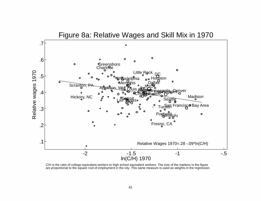
Appleton, WI AtlantaBoston

Charlotte

Chicago

Dallas

Denver

DetroitEl Paso

Fresno, CA

Greensboro

Hickory, NC

Honolulu

Houston

Las Vegas

Little Rock

Los AngelesMadison

Memphis

MinneapolisNYC

Philadelphia

Portland

St. Louis

San Francisco Bay Area

Scranton, PA

Seattle

Tucson

DC

Relative Wages 1970=.28 -.09*ln(C/H).1

.2

.3

.4

.5

.6

.7

Rel

ativ

e w

ages

197

0

-2 -1.5 -1 -.5ln(C/H) 1970

C/H is the ratio of college equivalent workers to high school equivalent workers. The size of the markers in the figureare proportional to the square root of employment in the city. This same measure is used as weights in the regression.

Figure 8a: Relative Wages and Skill Mix in 1970

41

Appleton, WI

Atlanta

Boston

Charlotte

Chicago

Colorado Springs

Dallas

DenverDetroit

El Paso

Fresno, CA

GreensboroHickory, NC

Honolulu

Houston

Las VegasLittle Rock Los Angeles

Madison

Memphis

Minneapolis

NYCPhiladelphia

Portland

St. Louis

San Francisco Bay Area

Scranton, PA

SeattleTucson

DC

Relative Wages 1980=.27 -.06*ln(C/H).1

.2

.3

.4

.5

.6

Rel

ativ

e w

ages

198

0

-1.5 -1 -.5ln(C/H) 1980

C/H is the ratio of college equivalent workers to high school equivalent workers. The size of the markers in the figureare proportional to the square root of employment in the city. This same measure is used as weights in the regression.

Figure 8b: Relative Wages and Skill Mix in 1980

42

Appleton, WI

Atlanta

Boston

Charlotte

Chicago

Colorado Springs

Dallas

DenverDetroit

El Paso

Fresno, CAGreensboro

Hickory, NC

Honolulu

Houston

Las Vegas

Little RockLos Angeles

Madison

Memphis

Minneapolis

NYCPhiladelphiaPortlandSt. LouisSan Francisco Bay Area

Scranton, PA

Seattle

Tucson

DC

Relative Wages 1990=.38 -.07*ln(C/H)

.1

.2

.3

.4

.5

.6

.7

Rel

ativ

e w

ages

199

0

-1.5 -1 -.5 0 .5ln(C/H) 1990

C/H is the ratio of college equivalent workers to high school equivalent workers. The size of the markers in the figureare proportional to the square root of employment in the city. This same measure is used as weights in the regression.

Figure 8c: Relative Wages and Skill Mix in 1990

43

Appleton, WI

Atlanta

Boston

Charlotte

ChicagoColorado Springs

Dallas

Denver

Detroit

El Paso

Fresno, CA

GreensboroHickory, NC

Honolulu

Houston

Las Vegas

Little Rock

Los Angeles

Madison

Memphis

Minneapolis

NYCPhiladelphia

Portland

St. Louis

San Francisco Bay Area

Scranton, PASeattle

Tucson

DC

Relative Wages 2000=.45 -.01*ln(C/H).2

.3

.4

.5

.6

.7

Rel

ativ

e w

ages

200

0

-1 -.5 0ln(C/H) 2000

C/H is the ratio of college equivalent workers to high school equivalent workers. The size of the markers in the figureare proportional to the square root of employment in the city. This same measure is used as weights in the regression.

Figure 8d: Relative Wages and Skill Mix in 2000

44

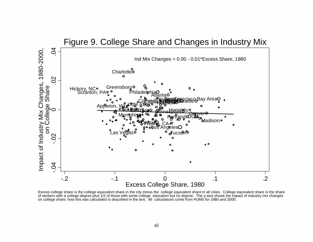
Hickory, NCScranton, PA

Appleton, WI

Charlotte

Greensboro

Las Vegas

MemphisEl PasoSt. Louis

Little Rock

Detroit

PhiladelphiaAtlantaChicago

Fresno, CA

DallasHoustonColorado SpringsNYC

Los Angeles

Boston

MinneapolisPortland

Tucson

Honolulu

Seattle

DCDenver

San Francisco Bay Area

Madison

Ind Mix Changes = 0.00 - 0.01*Excess Share, 1980-.0

4-.0

20

.02

.04

Impa

ct o

f Ind

ustry

Mix

Cha

nges

, 198

0-20

00,

on C

olle

ge S

hare

-.2 -.1 0 .1 .2Excess College Share, 1980

Excess college share is the college equivalent share in the city minus the college equivalent share in all cities. College equivalent share is the shareof workers with a college degree plus 1/2 of those with some college education but no degree. The y-axis shows the impact of industry mix changeson college share; how this was calculated is described in the text. All calculations come from PUMS for 1980 and 2000.

Figure 9. College Share and Changes in Industry Mix

45