En l’honneur de Jean Walrand The Next Wave in Networking … · 2019-06-27 · INTERFERENCE QUEUING ORKS NETW Wireless Spatial Birth-Death Pro cesses F. Baccelli UT Austin En l’honneur

✬ ✩

INTERFERENCE QUEUING NETWORKS

Wireless Spatial Birth-Death Pro esses

F. Ba elli

UT Austin

En l’honneur de Jean Walrand

The Next Wave in Networking ResearchSeptember 07, 2018, Berkeley

✫ ✪

✬ ✩1

Stru ture of the Le ture

Background and Motivation

Wireless Birth-Death Processeswith A. Sankararaman, IEEE Tr. IT, 63(6) 20171. Stability, 2. Clustering, 3. Quantitative results

Interference Queuing Networkswith S. Foss & A. Sankararaman, arXiv 1710.097971. Stability, 2. Minimal solution, 3. Initial condition

Interference Queuing Networks✫ ✪

✬ ✩2

Motivations in Wireless Networks

Lack of understanding and analysis of

Space-time interactions

– Static spatial setting well understood: Stochastic Geometry[FB, Blaszczyszyn 01]

– Churn taken into account in flow-based queuing[Bonald, Proutiere 06], [Shakkottai, De Veciana 07][Jiang, Walrand 09]

Contents of this lecture:

Models with such dynamics in stochastic geometry


✬ ✩3

I. Wireless Birth-Death Pro esses

Setting: Infrastructureless Wireless Network:Ad-hoc Networks, D2D Networks, IoT

Statistical assumptions: Markov Models:Poisson, Exponential

Mathematical tools:Point processes, Fluid


✬ ✩4


✬ ✩5

Sto hasti Network Model

S = [−Q,Q]× [−Q,Q]: torus where the wireless links live

Links: (Tx-Rx pairs)

Links: arrive as a PPP on IR× S with intensity λ:Prob. of a point arriving in space dx and time dt: λdxdt

Each Tx has an i.i.d. exponential file sizeof mean L bits to transmit to its Rx

A point exits after the Tx finishes transmitting its file

Φt: set of locations of links present at time t:

Φt = {x1, . . . ,xNt}, xi ∈ S


✬ ✩6

Interferen e and Servi e Rate

Interference seen at point x due to configuration Φ

I(x,Φ) =∑

xi∈Φ6=x

l(||x− xi||)

– Distance on the torus

– l(·): IR+ → IR+: path loss function

The speed of file transfer by link at x in configuration Φ is

R(x,Φ) = B log2

(

1 +1

N + I(x,Φ)

)

B,N Positive constants


✬ ✩7

B& D Master Equation

A point born at xp and time bp with file-size Lp dies at time

dp = inf

t > bp :

t∫

u=bp

R(xp,Φu)du ≥ Lp

Spatial Birth-Death Process

– Arrivals from the Poisson Rain

– Departures happen at file transfer completion


✬ ✩8

Properties of the Dynami s

The statistical assumptions imply that Φt is a Markov Pro-cess on the set of simple counting measures on S

Euclidean extension of the flow-level models of[Bonald, Proutiere 06], [Shakkottai, De Veciana 07]


✬ ✩9

Questions

Existence and uniqueness of the stationary regimes of Φt

Characterization of the stationary regime(s) if existence


✬ ✩10

Main Stability Results

a :=

∫

x∈S

l(||x||)dx

Theorem

– If λ > Bln(2)La, then Φt admits no stationary regime.

– If λ < Bln(2)La

, and r → l(r) bounded and monotone,

then Φt admits a unique stationary regime

Necessary condition by Palm calculus, Stochastic intensity

Sufficient condition by fluid limit

CorollaryFor the path-loss model l(r) = r−α, α ≥ 2, for all λ > 0, and allmean file sizes, the process Φt admits no stationary-regime


✬ ✩11

Main Qualitative Result

Φ stationary point-process on S with Palm distribution P0

ClusteringΦ is clustered if for all bounded, positive, non-increasingfunctions f(·) : R+ → R

+, the shot-noise

F(x,Φ) :=∑

y∈Φ\{x}

f(||y − x||)

satisfiesE0[F(0,Φ)] ≥ E[F(0,Φ)]


✬ ✩12

Main Qualitative Result (continued)

TheoremThe steady-state point process, when it exists, is clustered

Follows from Palm calculus + the FKG inequality

Interpretation of the resultThe steady-state interference measured at a uniformly ran-domly chosen point of is larger in mean than that at anuniformly random location of space.

Key Observation

– Dynamics Shapes Geometry

– Geometry Shapes Dynamics


✬ ✩13

0 5 10 150

5

10

15

A sample of Φ when λ = 0.99 and l(r) = (r + 1)−4.


✬ ✩14

Quantitative Results

Heuristics for the intensity of the steady-state process

1. Poisson heuristic βf - derived by neglecting clustering andassuming Poisson

2. Second-order heuristic βs based on a second-order cavityapproximation of the dynamics


✬ ✩15

Poisson Heuristi

Exact Rate Conservation Law:

λL = βE0Φ

[

log2

(

1 +1

N + I(0)

)]

.

Poisson Heur.: Largest solution to the fixed point equation:

λL =βf

ln(2)

∞∫

z=0

e−Nz(1− e−z)

ze−βf

∫

x∈S(1−e−zl(||x||))dxdz

Ignores the Palm effect and uses that if X,Y are non-negativeand independent,

E

[

ln

(

1 +X

Y + a

)]

=

∞∫

z=0

e−az

z(1− E[e−zX])E[e−zY]dz.

The Poisson heuristic is tight in heavy and light traffic


✬ ✩16

Se ond Order Heuristi

The intensity βs is given by

βs =λL

B log2

(

1 + 1N+Is

)

where Is is the smallest solution of the fixed-point equation

Is = λL

∫

x∈S

l(||x||)

B log2

(

1 + 1N+Is+l(||x||)

)dx


✬ ✩17

Second Order Heuristic (continued)

Rationale based on ρ2(x,y): second moment measure of Φ

Rate Conservation for ρ2: when considering Is as a constant

ρ2(x,y)1

LB log2

(

1 +1

N + Is + l(||x− y||)

)

= λβs

From the definition of second moment measure,

Is =

∫

x∈S

l(||x||)ρ2(0,x)

βsdx

which gives the fixed point equation for Is

The formula for βs follows from Rate Conservation for ρ1 = βs


✬ ✩18

0.4 0.5 0.6 0.7 0.8 0.9 1

0

5

10

15

20

25

30

λ / λc

β

Simulations

Second−Order Heuristic

Poisson Heuristic

95% confidence interval when l(r) = (r + 1)−4


✬ ✩19

II. Interferen e Queuing Networks

Aim: extension of dynamics to R2 (scalability)

Setting

– Discretization: queuing dynamics on a grid

– Low SINR: linearization of the log

Mathematical Tools

– Interacting particle systems

– Coupling from the past

– Rate conservation principle


✬ ✩20


✬ ✩21

Assumptions, Notation

Queue i at i ∈ Zd has state xi(t) ∈ N at time t

Arrivals to queues:i.i.d. Poisson processes of rate λ > 0

Interference sequence:{ai}i∈Zd, non-negative, symmetric (ai = a−i), and irreducible

Service discipline:generalized processor-sharing with rate of queue i at time t:

xi(t)∑

j∈Zd ajxi−j(t)


✬ ✩22

Stability, Minimal Stationary Regime

Stability: when starting the system empty at time 0, weakconvergence of the state of any finite set of queues as t → ∞

Theorem If

λ <1

∑

i∈Zd ai

– The network is stable

– The weak limit is the minimal stationary regime

Proof: CFP

The stability condition λ < 1∑

i∈Zdaiis sharp (current proof in

special cases only)


✬ ✩23

Quantitative Properties of Minimal Stationary Regime

Theorem The weak limit, when it exists, satisfies

E[x0] =λa0

1− λ∑

i∈Zd ai

In addition its coordinates (xi)i∈Zd are associated

Proof: RCP

Association: analogue of of clustering in the continuum

Remarkable fact: closed form for the mean for thisinfinite-dimensional, non-reversible, non-asymptotically in-dependent particle system


✬ ✩24

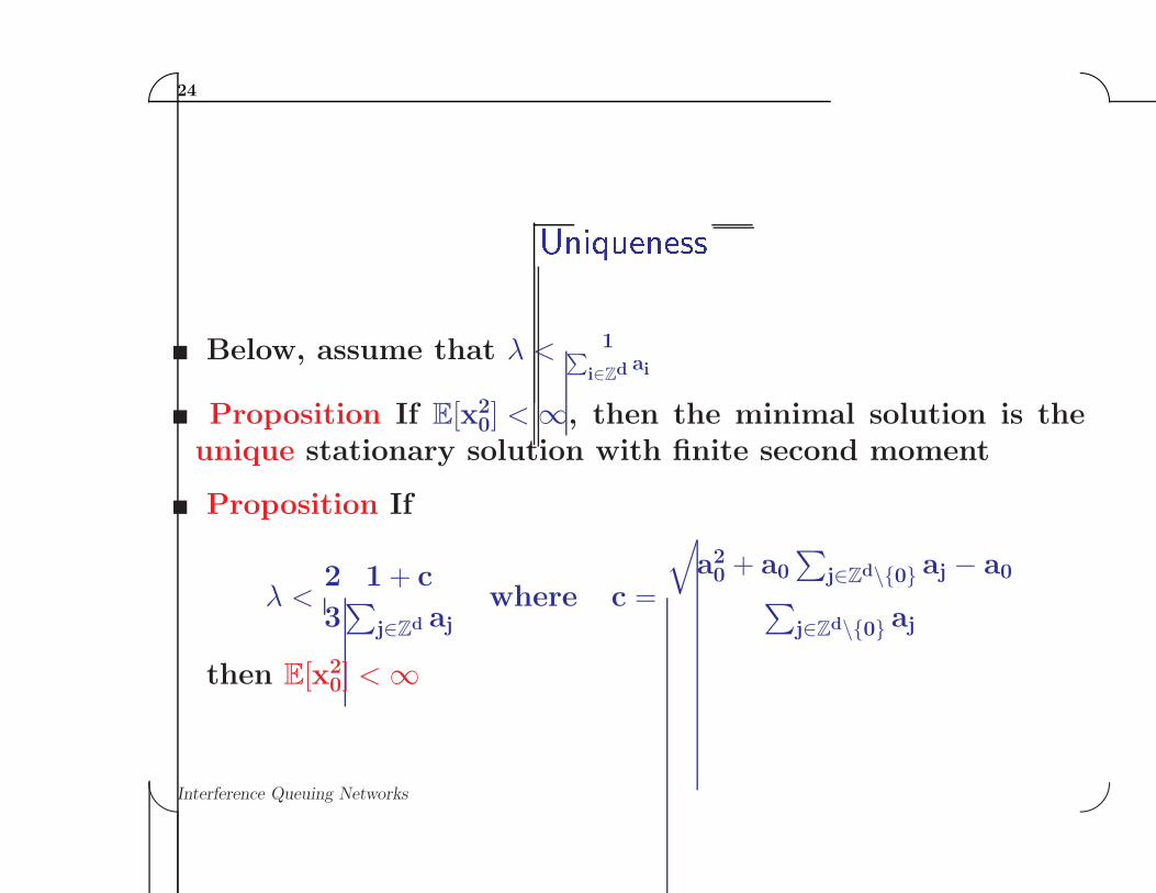
Uniqueness

Below, assume that λ < 1∑

i∈Zdai

Proposition If E[x20] < ∞, then the minimal solution is the

unique stationary solution with finite second moment

Proposition If

λ <2

3

1 + c∑

j∈Zd ajwhere c =

√

a20 + a0∑

j∈Zd\{0} aj − a0∑

j∈Zd\{0} aj

then E[x20] < ∞


✬ ✩25

Domain of Attra tion of the Minimal Solution

Theorem If λ < 23

1+c∑

j∈Zdaj

and the initial condition satisfies

supi∈Zd

xi(0) < ∞

then {xi(·)}i∈Zd converges weakly to the minimal stationarysolution

Theorem For d = 1, for all λ > 0, there exists

1. A deterministic sequence (αi)i∈Z such that if xi(0) ≥ αi forall i ∈ Z, then limt→∞ x0(t) = ∞ a.s.

2. A distribution ξ on N s.t. if {xi(0)}i∈Z is i.i.d. with marginaldistr. ξ, then limt→∞ x0(t) = ∞ a.s.


✬ ✩26

Summary

A new basic representation of space-time interactions inwireless networks

A generative model for clustering as assumed in simulationstandards

A new dynamic notion of capacity involving both queuingand IT

First exact analytical results in the low SINR case and goodheuristics in general

A new particle system dynamics with closed form althoughno reversibility, no asymptotic independence


✬ ✩27

Thanks Jean

MERCI JEAN POUR NOS PREMIERS ∼ 40 ANSD’INTERACTIONS AMICALES ET

SCIENTIFIQUES!


Documents

En l’honneur de Jean Walrand The Next Wave in Networking … · 2019-06-27 · INTERFERENCE QUEUING ORKS NETW Wireless Spatial Birth-Death Pro cesses F. Baccelli UT Austin En l’honneur