EMPIRICAL STUDY OF TWO HYPOTHESIS TEST METHODS FOR

EMPIRICAL STUDY OF TWO HYPOTHESIS TEST METHODS FOR COMMUNITY

STRUCTURE IN NETWORKS

A Thesis

Submitted to the Graduate faculty

of the

North Dakota State University

of Agriculture and Applied Science

By

Yehong Nan

In Partial Fulfillment of the Requirements

for the Degree of

MASTER OF SCIENCE

Major Program:

Applied Statistics

April 2019

Fargo, North Dakota

North Dakota State University

Graduate School

Title

Empirical study of two hypothesis test methods for community structure in networks

By

Yehong Nan

The Supervisory Committee certifies that this disquisition complies with North Dakota

State University’s regulations and meets the accepted standards for the degree of

MASTER OF SCIENCE

SUPERVISORY COMMITTEE:

Dr. Rhonda Magel

Chair

Dr. Mingao Yuan

Dr. Lu Liu

Approved:

April 30, 2019 Dr. Rhonda Magel

Date Department Chair

iii

ABSTRACT Many real-world network data can be formulated as graphs, where a binary relation exists

between nodes. One of the fundamental problems in network data analysis is community detection,

clustering the nodes into different groups. Statistically, this problem can be formulated as

hypothesis testing: under the null hypothesis, there is no community structure, while under the

alternative hypothesis, community structure exists. One is of the method is to use the largest

eigenvalues of the scaled adjacency matrix proposed by Bickel and Sarkar (2016), which works

for dense graph. Another one is the subgraph counting method proposed by Gao and Lafferty

(2017a), valid for sparse network. In this paper, firstly, we empirically study the BS or GL methods

to see whether either of them works for moderately sparse network; secondly, we propose a

subsampling method to reduce the computation of the BS method and run simulations to evaluate

the performance.

iv

ACKNOWLEDGEMENTS

I would like to thank my advisor, Dr. Mingao Yuan, for his excellent guidance and support,

great help and patience, and the most kindness throughout the course of this work.

My thanks also go to the members of my supervisory committee, Dr. Rhonda Magel and

Dr. Lu Liu, for their insightful advice and great support.

I would also like to thank my husband and my parents for their encouragement, inspiration,

and support.

I am grateful to all my friends, classmates, and teachers for their friendship, love, support,

and help during the course of my graduate studies.

Finally, I would like to thank the North Dakota State University and the Department of

Statistics for awarding me an opportunity for pursuing my Master Degree of Applied Statistics.

v

TABLE OF CONTENTS

ABSTRACT ................................................................................................................................... iii

ACKNOWLEDGEMENTS ........................................................................................................... iv

LIST OF TABLES ........................................................................................................................ vii

LIST OF FIGURES ..................................................................................................................... viii

1. INTRODUCTION ...................................................................................................................... 1

2. BACKGROUND ........................................................................................................................ 3

2.1. BS Test ................................................................................................................................. 4

2.1.1. Bickel and Sarkar (2016) .......................................................................................... 5

2.2. GL Test ................................................................................................................................. 5

2.2.1. Gao and Lafferty (2017a) ......................................................................................... 6

3. SUBSAMPLING METHOD FOR BS ....................................................................................... 8

4. SIMULATION-BASED COMPARISON ................................................................................ 10

4.1. Simulated size and power of GL Method ........................................................................... 10

4.2. Simulated size and power of BS Method ........................................................................... 13

4.3. Simulated size and power: degree-corrected SBM ............................................................ 15

4.4. Simulated size and power for degree-corrected SBM ........................................................ 17

4.5. Simulated size and power of subsampling method for BS ................................................. 17

5. SUMMARY .............................................................................................................................. 20

REFERENCES ............................................................................................................................. 21

APPENDIX A. R CODE FOR SIMULATED GL METHOD ..................................................... 24

APPENDIX B. R CODE FOR SIMULATED BS METHOD SBM ........................................... 26

APPENDIX C. R CODE FOR SIMULATED GL-W METHOD SIZE&POWER...................... 29

APPENDIX D. CODE FOR BS-W METHOD SIZE&POWER OF SBM .................................. 32

APPENDIX E. CODE FOR SUBSAMPLING-BS METHOD .................................................... 35

vi

APPENDIX F. CODE FOR CURVES ......................................................................................... 38

vii

LIST OF TABLES

Table Page

1. Simulated size and power of GL Method ................................................................................ 12

2. Simulated size and power BS Method SBM............................................................................ 14

3. Simulated size and power: degree-corrected SBM .................................................................. 16

4. Simulated size and power: BS method for degree-corrected SBM ......................................... 17

5. Simulated size and power subsampling method for BS ........................................................... 19

viii

LIST OF FIGURES

Figure Page

1. Simulated power of GL Method .............................................................................................. 11

2. Simulated size and power: degree-corrected SBM .................................................................. 15

3. Simulated size and power subsampling method for BS ........................................................... 18

1

1. INTRODUCTION

Many real-world data can be formulated as graphs, where a binary relation (edge) exists

between nodes. For example, in the Facebook, each user is a node and the friendship between two

users form an edge; in the coauthored-ship data, each author of a paper is a node, and an edge

exists between two authors if they coauthored one paper. These data are called network data and

the analysis of these data is named the network data analysis. One of the fundamental questions is

community detection, grouping the nodes into different clusters. In the literature, there are various

algorithms that output the clusters given the network data as an input. However, one may wonder

whether the output makes sense or not, that is, whether any community structure truly exists or

not. Statistically, this is equivalent to testing the null hypothesis that there is no community

structure against the alternative hypothesis that community structure exists. There are several

statistical testing procedures proposed based on the sparsity of the network in the literatures

(Bickel and Sarkar (2016); Gao and Lafferty (2017a); Zhao Levina and Zhu (2011)). For example,

the spectral method (BS) proposed by Bickel and Sarkar (2016) works for dense graph, while the

subgraph-counting method (GL) proposed by Gao and Lafferty works for relatively sparse network

(Gao and Lafferty (2017a), Gao and Lafferty (2017b)) and the likelihood-ratio type test proposed

by Yuan, Feng and Shang (2019) is valid for the extremely sparse network. For moderately dense

network, to our knowledge, there is no existing test procedures. In this paper, firstly, we

empirically study the BS or GL methods to see whether either of them works for moderately dense

network; secondly, we propose a subsampling method to reduce the computation of the BS method

and run simulations to evaluate the performance.

2

The rest of the paper is organized as follows. In section 2, we briefly introduce the SBM

models, the BS or GL methods, and present the subsampling method for BS test. In section 3, we

present the simulation results, followed by a summary in section 4.

3

2. BACKGROUND

The network data can be formulated as a graph. Let 𝐺𝑛 = (𝑉, 𝐸) be a graph with 𝑛 nodes,

where 𝑉 is the vertex set and 𝐸 is the edge set. Let 𝐴 be the adjacency matrix, that is, 𝐴𝑖𝑗 = 1 if

(ⅈ, 𝑗) is an edge, 𝐴𝑖𝑗 = 0, otherwise. In the research of network data, SBM is one of the most

popular and tractable models, it plays an important role in providing a supporting ground to study

many crucial problems, such as clustering and community detection (Amini, Chen and Bickel

(2013); Amini and Levina (2018); Neeman and Netrapalli (2014); Sarkar and Bickel (2015);

Bickel and Chen (2009); Zhao Levina and Zhu (2012)) and the goodness-of-fit of SBMs (Bickel

and Sarkar (2016); Lei (2016); Montanari and Sen (2016); Banerjee and Ma (2017); Banerjee

(2018); Gao and Lafferty (2017a). Gao and Lafferty (2017b)) or various phase transition

phenomena (Abbe (2017)). The SBM is defined as follows. Let 𝐺𝐾 (𝑛,𝐵

𝑛) be a SBM, where 𝐾 is

the number of communities and 𝐵 is a 𝐾 × 𝐾 symmetric matrix with positive entries; let 𝑍 be a

random uniform lable assignment taking value in {1,2, ⋯ , 𝐾}. given 𝑍, the edge probability is

defined as ℙ ( 𝐴𝑖𝑗= 1| Z) = 𝐵𝑧𝑖𝑧𝑗

𝑛 ; besides, 𝐴𝑖𝑗 are assumed to be conditionally independent. In this

paper, we focus on the case where 𝐵11 =𝐵22 =𝑎 , 𝐵12 =𝐵21 =𝑏 . Here, 𝑎

𝑛 represents the within

community probability and 𝑏

𝑛 is the between community probability. And we assume 𝑎 > 𝑏, that

is, edge density in intra-community is larger than inter-community. The 𝐸𝑟𝑑�̈� − 𝑅é𝑛𝑦ⅈ model is

a counterpart of SBM, where any two nodes are connected with probability 𝑝 . Note that

the 𝐸𝑟𝑑�̈� − 𝑅é𝑛𝑦ⅈ model only has one cluster. If the edge probability 𝑝 is a fixed constant, the

network is said to be dense. If 𝑝 goes to zero at the order 1

𝑛, we say it is extremely sparse. When

𝑝 =𝑎𝑛

𝑛 for some positive sequence 𝑎𝑛 of smaller order than 𝑛 but goes to infinity as 𝑛, we say the

network is moderately sparse or dense.

4

In practice, the SBM may not be a good fit of the real data. For example, in the Facebook

user data, each user may have different number of friends; in the coauthorship data, the number of

coauthors a researcher may vary a lot. The degree-corrected SBM is one generalization of it. The

advantage is that it allows for heterogeneity of degrees in the network. Let 𝑊𝑖(1 ≤ ⅈ ≤ 𝑛) be iid

random variables with 𝐸𝑊2 = 1 and 𝑍𝑖~𝑈𝑛ⅈ𝑓𝑜𝑟𝑚([k]). In the degree-corrected stochastic block

model, the adjacency matrix component 𝐴𝑖𝑗 | 𝜃𝑖𝑗~𝐵𝑒𝑟𝑛𝑜𝑢𝑙𝑙ⅈ(𝜃ⅈ𝑗) , where 𝜃𝑖𝑗 = 𝑊𝑖𝑊𝑗((𝑎 −

𝑏)𝐼[𝑧𝑖 = 𝑧𝑗] + 𝑏), where 𝑎 represents the within-cluster edge probability and 𝑏 is the between-

cluster edge probability. Conditional on 𝑊 and 𝑍 , 𝐴𝑖𝑗 are assumed to be independent. Note that if

we take 𝑊𝑖 = 1, then the degree-corrected SBM is just the usual SBM.

Whether community structure exists in a network can be formulated as the hypothesis

problems: under the null hypothesis, the network is generated from the 𝐸𝑟𝑑�̈� − 𝑅é𝑛𝑦ⅈ model,

while under the alternative hypothesis, the network is generated from the corresponding SBM or

degree-corrected SBM. There are several statistical testing procedures proposed based on the

sparsity of the network in the literature. For dense network, Bickel and Sarkar (2016) proposed the

spectral method (BS); for relatively sparse network, Gao and Lafferty(2017b) proposed the

subgraph-counting method (GL). In the following, we introduce the two methods in detail.

2.1. BS Test

By using the largest eigenvalues of the scaled adjacency matrix, Bickel and Sarkar (2016)

proposed a test statistic to test community structures. Let 𝐴 be the adjacency matrix of a network.

Suppose that there are no self-loops, that is, 𝐴𝑖𝑖 = 0, ∀ⅈ. Under the 𝐸𝑟𝑑�̈� − 𝑅é𝑛𝑦ⅈ model, define

𝑃 as follows,

𝑃 = 𝑛𝑝ⅇⅇ𝑇 – 𝑝𝐼,

5

where 𝑒 is a length 𝑛 vector with 𝑒𝑖 = 1/√𝑛 , ∀ⅈ , and 𝐼 is the 𝑛 × 𝑛 identity matrix. Then

we scale the 𝐴 as follows,

�̃�′ =𝐴−�̂�

√(𝑛−1)𝑝(1−𝑝) ,

where �̂� = 𝑛�̂�ⅇⅇ𝑇 − �̂�𝐼,�̂� =𝛴𝐴𝑖𝑗

𝑛(𝑛−1). Let

𝜃 = 𝑛23(𝜆1(�̃�′) − 2) .

Here, λ1 is the largest eigen-values of a matrix. Bickel and Sarkar get the following asymptotic

distribution of 𝜃.

2.1.1. Bickel and Sarkar (2016)

Under the 𝐸𝑟𝑑�̈� − 𝑅é𝑛𝑦ⅈ model, for fixed 𝑝 , 𝜃 converges in distribution to the Tracy-

Widom law with index 1, 𝑇𝑊1.

Based on Theorem 2.1.1, we reject the null hypothesis if 𝜃 > 𝑇𝑊1,1−𝛼, where 𝑇𝑊1,1−𝛼 is

the (1 − 𝛼)100% quantile.

2.2. GL Test

By using relations between the observed frequencies of small subgraphs, Gao and Lafferty

proposed a subgraph counting method to test for the existence of communities (Gao and Lafferty

(2017a)). Consider the population edge, vee, and triangle probabilities

𝐸 = ℙ(𝐴12 = 1),

𝑉 = ℙ(𝐴12𝐴13 = 1),

𝑇 = ℙ(𝐴12𝐴13𝐴23 = 1).

Under the degree-corrected SBM, direct computation yields

𝑋𝑒𝑧 ≡ 𝑇 − (𝑉

𝐸)

3

=(𝑘−1)(𝑎−𝑏)3

𝑘3 .

6

Clearly, a good property of this quantity is that it vanishes under the null hypothesis while

it is not zero under the alternative hypothesis. Hence 𝑋𝑒𝑧 can be used to distinguish the null

hypothesis and the alternative hypothesis and the empirical version of it is a reasonable test statistic.

Denote

�̂� =1

(𝑛𝑛)

∑ 𝐴𝑖�̇�1≤ⅈ≤𝑗≤𝑛

,

�̂� =1

(𝑛3)

∑𝐴𝑖𝑗𝐴𝑖𝑙+𝐴𝑖𝑗𝐴𝑗𝑙+𝐴𝑖𝑙𝐴𝑗𝑙

31≤ⅈ<𝑗<𝑙≤𝑛 ,

�̂� =1

(𝑛3)

∑ 𝐴𝑖𝑗𝐴𝑗𝑙𝐴𝑙𝑖1≤ⅈ<𝑗<𝑙≤𝑛

,

�̂�, �̂�, �̂� are estimates of 𝐸, 𝑉, 𝑇 respectively. Define

�̂�𝑒𝑧 ≡ �̂� − (�̂� ∕ �̂�)3 .

The following theorem gives the asymptotic distribution of �̂�𝑒𝑧 under the null hypothesis and then

we can set threshold at the given significance level.

2.2.1. Gao and Lafferty (2017a)

Assume 𝐸𝑊4 = 𝑂(1) and 𝑛−1 ≪ 𝑎 , 𝑏 ≪ 𝑛−2

3. Let

𝛿 = 𝑙ⅈ𝑚𝑛

(𝑘 − 1)(𝑎 − 𝑏)

√6((

𝑛

𝑘(𝑎 + (𝑘 − 1)𝑏))

32

) .

Then the following holds,

√(

𝑛3)�̂�𝑒𝑧

√�̂� → 𝑁(𝛿, 1),

√(𝑛3)�̂�𝑒𝑧

√(𝑉∕�̂�)3 → 𝑁(𝛿, 1),

2√(𝑛3

)(√�̂� − (�̂� ∕ �̂�)3

2⁄→ 𝑁(𝛿, 1).

7

Theorem 2.2.1. (Gao and Lafferty (2017a)) shows that the asymptotic distribution of testing

statistic is the standard normal distribution. We can get the rejection region based the asymptotic

distribution. Note that the GL method works for relatively sparse networks, that is, 𝑛−1 ≪ 𝑎, 𝑏 ≪

𝑛−2

3 . The power of the GL test can attain 1 if the sample size and 𝛿 go to infinity (Gao and Lafferty

(2017a)).

8

3. SUBSAMPLING METHOD FOR BS

Note that the BS method requires the eigenvalue of the adjacency matrix. For large

network data, it’s impossible or at least time-consuming to calculate the eigenvalue. To reduce the

computation time, we propose a subsampling method as follows. Firstly, we randomly and

uniformly sample 𝑟 × 𝑛 indexes from [𝑛] = {1,2, . . . , 𝑛} without replacement. Here 𝑟 is a number

between 0 and 1. If 𝑟 is equal to 1, then all the original nodes are sampled. When 𝑟 is close to zero,

then only a small portion of the original nodes are sampled. Hence 𝑟 controls the proportion of

nodes we want to sample. Denote by 𝑆 the index set, say, 𝑆={1,2, . . . , 𝑟𝑛}. Then we apply the BS

method to the graph induced by 𝑆, that is, to the induced adjacency matrix 𝐴𝑠𝑠. For example, if

𝑆={1,2, . . . , 𝑟𝑛}, then 𝐴𝑠𝑠 is just the first 𝑟𝑛 rows and columns of the original adjacency matrix 𝐴.

To make the test based on subsample useful, we need to derive the asymptotic distribution of 𝜃𝑠,

the test statistic calculated based on 𝐴𝑠𝑠. Actually, it’s easy to see that Theorem 2.1.1. (Bickel and

Sarkar (2016)) still holds for 𝜃𝑠 . The basic idea behind this is that if 𝐴 is generated from an

𝐸𝑟𝑑�̈� − 𝑅é𝑛𝑦ⅈ model, 𝐴𝑠𝑠 is also generated from an 𝐸𝑟𝑑�̈� − 𝑅é𝑛𝑦ⅈ model. Suppose for 𝐴, the

edge probability is 𝑝0, then the edge probability is still 𝑝0 for 𝐴𝑠𝑠. The only difference is that there

are 𝑛 nodes for 𝐴 but 𝑟𝑛 nodes for 𝐴𝑠𝑠. Hence 𝐴𝑠𝑠 is still a dense network as 𝐴. Then Theorem

2.1.1. (Bickel and Sarkar (2016)) still holds.

For given significance level 𝛼, we can construct the rejection region. We reject the null

hypothesis if 𝜃𝑠 > 𝑇𝑊1,1−𝛼, where 𝑇𝑊1,1−𝛼 is the (1 − 𝛼)100% quantile of the Tracy-Widom

law with index 1. In terms of computation time, if 𝑟 is a constant, then the reduced time is moderate.

However, if we allow 𝑟 to approach zero, in this case, the reduced time is significant. But there

might be a trade-off between running time and power of the test. Larger 𝑟 implies larger power

9

but slower computation; smaller 𝑟 will save more time but sacrifices some power. In practice, we

recommend to use the largest 𝑟 within the computation budget.

10

4. SIMULATION-BASED COMPARISON

In this simulation, let =𝑎𝑛

𝑛 , 𝑏 =

𝑏𝑛

𝑛, where 𝑎𝑛 and 𝑏𝑛 are given in the tables and they

control the sparsity of the network. If 𝑎𝑛 = 𝑐1𝑛, 𝑏𝑛 = 𝑐2𝑛 for constants 𝑐1 and 𝑐2 between zero

and one, then the network is dense. When (𝑎𝑛, 𝑏𝑛)= (𝑐3𝑛λ , 𝑐4𝑛μ) for some positive constants

𝑐3, 𝑐4 and 0 < λ < 1, 0 < μ < 1, we say the network is moderately sparse. For the subsample

method, the subsample size is 𝑟𝑛, where 0 < 𝑟 < 1. In this simulation, we use 𝑟=0.05, 0.10, 0.15,

0.20. We use the nominal significance level 𝑎 = 0.05 and generate the SBM with 𝑘 = 2

communities with or without degree correction. Both size and power are calculated as proportions

of rejections based on 500 independent experiments. To simulate the size, we generate the data

from the 𝐸𝑟𝑑�̈� − 𝑅é𝑛𝑦ⅈ model with probability 𝑎𝑛+𝑏𝑛

2𝑛. To evaluate the tendency of the power, we

increase 𝑎𝑛 with 𝑏𝑛 fixed. This will make the gap between 𝑎𝑛 and 𝑏𝑛 enlarge and the power is

expected to increase.

4.1. Simulated size and power of GL Method

Table 1 summarizes the size and power of GL method with various 𝑎𝑛 and 𝑏𝑛. In the first

column, 𝑘 means the number of community and in our simulation, we used 𝑘 = 2. In the second

column, we present the within-community and between-community probabilities 𝑎𝑛 , 𝑏𝑛 . The

sample size 𝑛 ranges from 200 to 500. From the R output, almost all the simulated sizes are close

to the nominal level 0.05, while the sizes in the last three rows are a little far away from 0.05. For

the larger 𝑎𝑛 and 𝑏𝑛 , we find the size are not close to 0.05. We omit the result. This is consistent

with the theory that the test only works for relatively sparse network, that is, 1 <<𝑎𝑛, 𝑏𝑛 << 𝑛−1

3.

For fixed 𝑎𝑛 and 𝑏𝑛 , when the sample size increases, the power also increases. For

example, when (𝑎𝑛, 𝑏𝑛)= (8𝑛0.2 , 𝑛0.2), the power for 𝑛 = 200 is 0.714, which increases to 0.914

11

when 𝑛 = 500. For fixed 𝑛, the power increases as the differences of 𝑎𝑛 and 𝑏𝑛 increases. For

instance, 𝑛 = 500 , (𝑎𝑛, 𝑏𝑛)= (2𝑛0.2 , 𝑛0.2), the power is 0.018, when (𝑎𝑛, 𝑏𝑛)= (8𝑛0.2 , 𝑛0.2),

the power is 0.914. All these patterns are clearly presented in Figure 1 for (𝑎𝑛, 𝑏𝑛)= (2𝑛0.2 ,

𝑛0.2), (4𝑛0.2 , 𝑛0.2), (8𝑛0.2 , 𝑛0.2).

Figure 1. Simulated power of GL Method

12

Table 1. Simulated size and power of GL Method

(an , bn)

n=200

GL(size)power

n=300

GL(size)power

n=400

GL(size)power

n=500

GL(size)power

k=2 (2log(n), log(n))

(4log(n), log(n))

(8log(n), log(n))

(0.044) 0.038

(0.024) 0.434

(0.024) 1.000

(0.036) 0.024

(0.032) 0.482

(0.024) 1.000

(0.058) 0.036

(0.034) 0.600

(0.038) 1.000

(0.048) 0.036

(0.030) 0.594

(0.040) 1.000

k=2 (2n0.1 , n0.1)

(4n0.1 , n0.1)

(8n0.1 , n0.1)

(0.072) 0.012

(0.050) 0.036

(0.042) 0.172

(0.078) 0.012

(0.028) 0.030

(0.038) 0.204

(0.062) 0.012

(0.054) 0.034

(0.048) 0.222

(0.062) 0.004

(0.058) 0.046

(0.058) 0.242

k=2 (2n0.2 , n0.2)

(4n0.2 , n0.2)

(8n0.2 , n0.2)

(0.046) 0.024

(0.034) 0.080

(0.024) 0.714

(0.052) 0.024

(0.040) 0.110

(0.044) 0.828

(0.054) 0.022

(0.038) 0.120

(0.048) 0.858

(0.044) 0.018

(0.042) 0.148

(0.036) 0.914

k=2 (2n0.3 , n0.3)

(4n0.3 , n0.3)

(8n0.3 , n0.3)

(0.030) 0.000

(0.040) 0.310

(0.010) 1.000

(0.060) 0.020

(0.030) 0.510

(0.010) 1.000

(0.080) 0.040

(0.020) 0.540

(0.030) 1.000

(0.054) 0.050

(0.030) 0.696

(0.032) 1.000

k=2 (2n0.4 , n0.4 )

(4n0.4 , n0.4)

(8n0.4 , n0.4)

(0.020) 0.030

(0.010) 0.980

(0.010) 1.000

(0.030) 0.070

(0.020) 0.980

(0.030) 1.000

(0.020) 0.070

(0.060) 1.000

(0.020) 1.000

(0.034) 0.082

(0.032) 1.000

(0.016) 1.000

13

4.2. Simulated size and power of BS Method

Table 2 shows the size and power of Bickel and Sarkar (BS) method with estimated 𝑎𝑛 and

𝑏𝑛. Firstly, when 𝑎𝑛 < 0.12𝑛 and 𝑏𝑛 < 0.10𝑛 ,we can see the simulated sizes are all significantly

larger than 0.05, which implies the BS method doesn’t work for sparse network(small edge

probability). In this case, it doesn’t make sense to run the power simulation, so we omit it (the star

sign). Secondly, when 𝑎𝑛 > 0.15𝑛 and 𝑏𝑛 > 0.10𝑛 all the sizes are close to 0.05, which implies

the BS method is valid for dense network. Thirdly, for fixed 𝑎𝑛 and 𝑏𝑛,when sample size increases,

the power also increases. For example, (𝑎𝑛, 𝑏𝑛) = (0.15𝑛, 0.10𝑛), the power increases from 0.220

at 𝑛 = 200 to 0.998 at 𝑛 = 500. For fixed 𝑛, when the gap between 𝑎𝑛 and 𝑏𝑛 enlarges, the power

increases.

14

Table 2. Simulated size and power BS Method SBM

(an , bn)

n=200

BS(size) power

n=300

BS(size) power

n=400

BS(size) power

n=500

BS(size) power

K=2 (0.02n, 0.01n)

(0.04n, 0.01n)

(0.06n, 0.01n)

(0.08n, 0.01n)

(0.10n, 0.01n)

(0.10n, 0.03n)

(0.10n, 0.05n)

(0.10n, 0.07n)

(0.10n, 0.09n)

(0.12n, 0.10n)

(0.994) *

(0.920) *

(0.640) *

(0.450) *

(0.244) *

(0.234) *

(0.160) *

(0.100) *

(0.090) *

(0.110) *

(0.984) *

(0.854) *

(0.610) *

(0.460) *

(0.290) *

(0.176) *

(0.116) *

(0.124) *

(0.114) *

(0.070)*

(1.000) *

(0.810) *

(0.670) *

(0.430) *

(0.220) *

(0.130) *

(0.190) *

(0.080) *

(0.080) *

(0.110) *

(1.000) *

(0.850) *

(0.620) *

(0.320) *

(0.250) *

(0.300) *

(0.140) *

(0.170) *

(0.080) *

(0.050) *

K=2 (0.15n, 0.10n)

(0.20n, 0.10n)

(0.30n, 0.10n)

(0.40n, 0.10n)

(0.30n, 0.20n)

(0.40n, 0.20n)

(0.050) 0.220

(0.040) 1.000

(0.030) 1.000

(0.000) 1.000

(0.020) 0.840

(0.030) 1.000

(0.080) 0.600

(0.070) 1.000

(0.050) 1.000

(0.040) 1.000

(0.030) 1.000

(0.040) 1.000

(0.050) 0.960

(0.050) 1.000

(0.060) 1.000

(0.000) 1.000

(0.010) 1.000

(0.010) 1.000

(0.050) 0.998

(0.050) 1.000

(0.080) 1.000

(0.030) 1.000

(0.030) 1.000

(0.020) 1.000

15

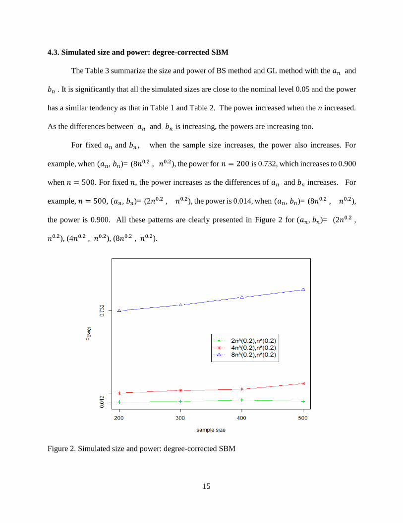
4.3. Simulated size and power: degree-corrected SBM

The Table 3 summarize the size and power of BS method and GL method with the 𝑎𝑛 and

𝑏𝑛 . It is significantly that all the simulated sizes are close to the nominal level 0.05 and the power

has a similar tendency as that in Table 1 and Table 2. The power increased when the 𝑛 increased.

As the differences between 𝑎𝑛 and 𝑏𝑛 is increasing, the powers are increasing too.

For fixed 𝑎𝑛 and 𝑏𝑛 , when the sample size increases, the power also increases. For

example, when (𝑎𝑛, 𝑏𝑛)= (8𝑛0.2 , 𝑛0.2), the power for 𝑛 = 200 is 0.732, which increases to 0.900

when 𝑛 = 500. For fixed 𝑛, the power increases as the differences of 𝑎𝑛 and 𝑏𝑛 increases. For

example, 𝑛 = 500, (𝑎𝑛, 𝑏𝑛)= (2𝑛0.2 , 𝑛0.2), the power is 0.014, when (𝑎𝑛, 𝑏𝑛)= (8𝑛0.2 , 𝑛0.2),

the power is 0.900. All these patterns are clearly presented in Figure 2 for (𝑎𝑛, 𝑏𝑛)= (2𝑛0.2 ,

𝑛0.2), (4𝑛0.2 , 𝑛0.2), (8𝑛0.2 , 𝑛0.2).

Figure 2. Simulated size and power: degree-corrected SBM

16

Table 3. Simulated size and power: degree-corrected SBM

(an , bn)

n=200

GL(size) power

n=300

GL(size) power

n=400

GL(size) power

n=500

GL(size) power

K=2 (log(n), log(n))

(2log(n), log(n))

(4log(n), log(n))

(8log(n), log(n))

(0.046) 0.012

(0.026) 0.016

(0.028) 0.402

(0.014) 0.998

(0.048) 0.014

(0.042) 0.036

(0.040) 0.454

(0.048) 1.000

(0.040) 0.024

(0.056) 0.042

(0.024) 0.560

(0.038) 1.000

(0.046) 0.024

(0.036) 0.028

(0.036) 0.610

(0.034) 1.000

K=2 (n0.1 , n0.1)

(2n0.1 , n0.1)

(4n0.1 , n0.1)

(8n0.1 , n0.1)

(0.104) 0.012

(0.098) 0.012

(0.040) 0.040

(0.046) 0.164

(0.134) 0.012

(0.068) 0.020

(0.038) 0.046

(0.044) 0.210

(0.168) 0.012

(0.054) 0.012

(0.036) 0.044

(0.038) 0.240

(0.198) 0.006

(0.074) 0.012

(0.050) 0.030

(0.032) 0.228

K=2 (n0.2 , n0.2)

(2n0.2 , n0.2)

(4n0.2 , n0.2)

(8n0.2 , n0.2)

(0.042) 0.014

(0.054) 0.012

(0.044) 0.082

(0.022) 0.732

(0.066) 0.010

(0.046) 0.016

(0.038) 0.104

(0.034) 0.778

(0.046) 0.018

(0.066) 0.028

(0.034) 0.114

(0.036) 0.838

(0.042) 0.014

(0.038) 0.018

(0.052) 0.158

(0.028) 0.900

K=2 (n0.3 , n0.3)

(2n0.3 , n0.3)

(4n0.3 , n0.3)

(8n0.3 , n0.3)

(0.036) 0.012

(0.046) 0.026

(0.022) 0.344

(0.024) 0.996

(0.340) 0.018

(0.020) 0.026

(0.022) 0.464

(0.050) 0.998

(0.040) 0.010

(0.036) 0.024

(0.044) 0.566

(0.018) 1.000

(0.054) 0.022

(0.040) 0.038

(0.044) 0.660

(0.044) 1.000

K=2 (n0.4, n0.4 )

(2n0.4, n0.4 )

(4n0.4 , n0.4)

(8n0.4 , n0.4)

(0.026) 0.022

(0.040) 0.062

(0.016) 0.904

(0.034) 1.000

(0.046) 0.018

(0.030) 0.052

(0.028) 0.986

(0.042) 1.000

(0.052) 0.010

(0.030) 0.084

(0.050) 0.998

(0.042) 1.000

(0.052) 0.036

(0.032) 0.112

(0.044) 0.998

(0.052) 1.000

17

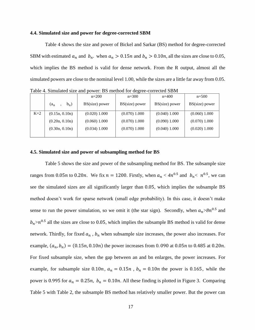
4.4. Simulated size and power for degree-corrected SBM

Table 4 shows the size and power of Bickel and Sarkar (BS) method for degree-corrected

SBM with estimated 𝑎𝑛 and 𝑏𝑛. when 𝑎𝑛 > 0.15𝑛 and 𝑏𝑛 > 0.10𝑛, all the sizes are close to 0.05,

which implies the BS method is valid for dense network. From the R output, almost all the

simulated powers are close to the nominal level 1.00, while the sizes are a little far away from 0.05.

Table 4. Simulated size and power: BS method for degree-corrected SBM

(an , bn)

n=200

BS(size) power

n=300

BS(size) power

n=400

BS(size) power

n=500

BS(size) power

K=2 (0.15n, 0.10n)

(0.20n, 0.10n)

(0.30n, 0.10n)

(0.020) 1.000

(0.060) 1.000

(0.034) 1.000

(0.070) 1.000

(0.070) 1.000

(0.070) 1.000

(0.040) 1.000

(0.090) 1.000

(0.040) 1.000

(0.060) 1.000

(0.070) 1.000

(0.020) 1.000

4.5. Simulated size and power of subsampling method for BS

Table 5 shows the size and power of the subsampling method for BS. The subsample size

ranges from 0.05𝑛 to 0.20𝑛. We fix 𝑛 = 1200. Firstly, when 𝑎𝑛 < 4𝑛0.5 and 𝑏𝑛< 𝑛0.5, we can

see the simulated sizes are all significantly larger than 0.05, which implies the subsample BS

method doesn’t work for sparse network (small edge probability). In this case, it doesn’t make

sense to run the power simulation, so we omit it (the star sign). Secondly, when 𝑎𝑛>8𝑛0.5 and

𝑏𝑛>𝑛0.5 all the sizes are close to 0.05, which implies the subsample BS method is valid for dense

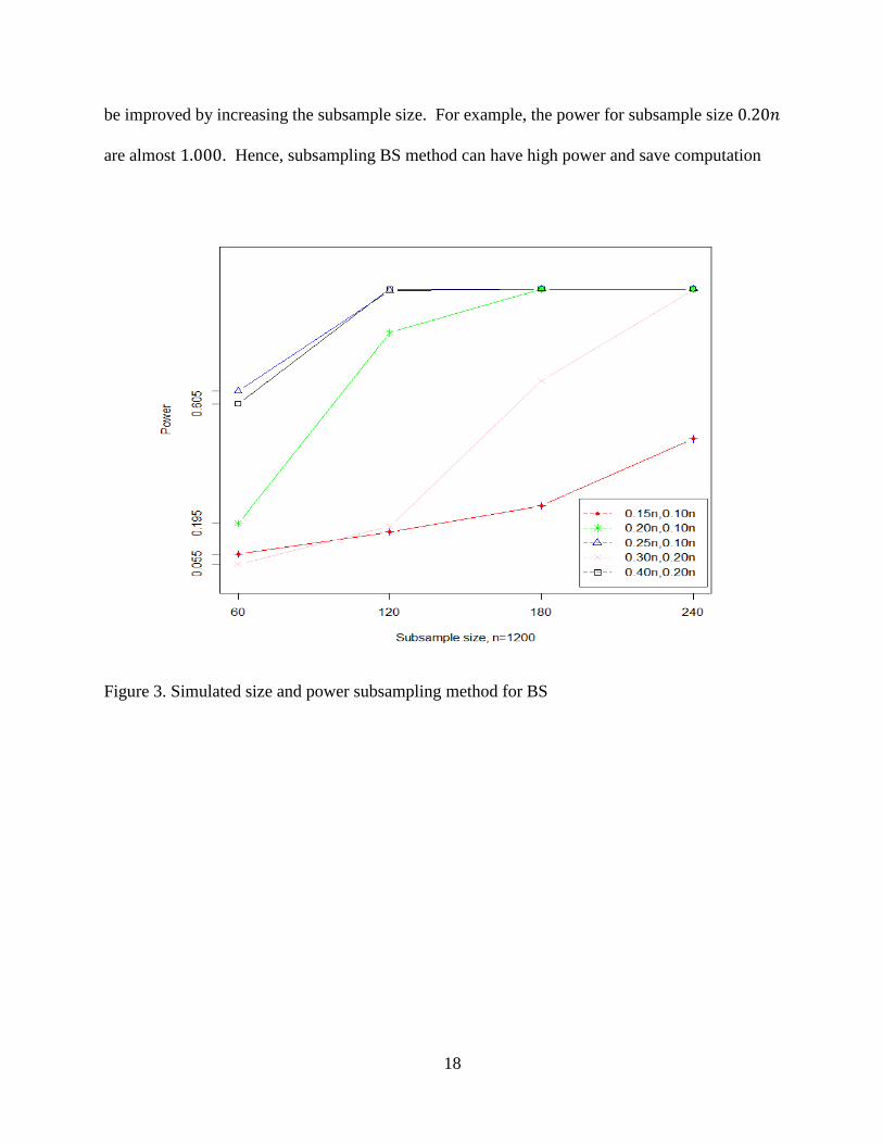
network. Thirdly, for fixed 𝑎𝑛 , 𝑏𝑛 when subsample size increases, the power also increases. For

example, (𝑎𝑛, 𝑏𝑛) = (0.15𝑛, 0.10𝑛) the power increases from 0. 090 at 0.05𝑛 to 0.485 at 0.20𝑛.

For fixed subsample size, when the gap between an and bn enlarges, the power increases. For

example, for subsample size 0.10𝑛 , 𝑎𝑛 = 0.15𝑛 , 𝑏𝑛 = 0.10𝑛 the power is 0.165 , while the

power is 0.995 for 𝑎𝑛 = 0.25𝑛, 𝑏𝑛 = 0.10𝑛. All these finding is plotted in Figure 3. Comparing

Table 5 with Table 2, the subsample BS method has relatively smaller power. But the power can

18

be improved by increasing the subsample size. For example, the power for subsample size 0.20𝑛

are almost 1.000. Hence, subsampling BS method can have high power and save computation

Figure 3. Simulated size and power subsampling method for BS

19

Table 5. Simulated size and power subsampling method for BS

(an , bn)

0.05n

(size) power

0.10n

(size) power

0.15n

(size) power

0.20n

(size) power

K=2 (2n0.3 , n0.3)

(4n0.3 , n0.3)

(8n0.3 , n0.3)

(0.972) *

(0.896) *

(0.642) *

(1.000) *

(0.968) *

(0.748) *

(1.000) *

(0.978) *

(0.732) *

(1.000) *

(0.982) *

(0.746) *

K=2 (2n0.5 , n0.5)

(4n0.5 , n0.5)

(8n0.5 , n0.5)

(0.380) *

(0.170) *

(0.058) 1.000

(0.452) *

(0.210) *

(0.048) 1.000

(0.466) *

(0.164) *

(0.070) 1.000

(0.488) *

(0.190) *

(0.054) 1.000

K=2 (2n0.7 , n0.7)

(4n0.7 , n0.7)

(8n0.7 , n0.7)

(0.030) 0.270

(0.020) 1.000

(0.010) 1.000

(0.032) 1.000

(0.024) 1.000

(0.008) 1.000

(0.030) 1.000

(0.026) 1.000

(0.014) 1.000

(0.012) 1.000

(0.012) 1.000

(0.012) 1.000

K=2 (0.15n, 0.10n)

(0.20n, 0.10n)

(0.25n, 0.10n)

(0.30n, 0.20n)

(0.40n, 0.20n)

(0.038) 0.090

(0.036) 0.195

(0.026) 0.650

(0.016) 0.055

(0.018) 0.605

(0.078) 0.165

(0.030) 0.850

(0.022) 0.995

(0.016) 0.185

(0.024) 1.000

(0.076) 0.255

(0.062) 1.000

(0.046) 1.000

(0.020) 0.685

(0.014) 1.000

(0.070) 0.485

(0.036) 1.000

(0.056) 1.000

(0.016) 0.995

(0.012) 1.000

20

5. SUMMARY

In this paper, we empirically compare two statistical testing procedures for testing

community structures in network data. The GL method is based on the frequencies of triangles,

vees and edges, while the BS method is to use the eigen-values of the centered and scaled

adjacency matrix. Theoretically, the BS method works for dense network and the GL method is

valid for moderately sparse network. By our simulation study, when the network is dense, that is,

the edge probability is far away from zero (larger than 0.15 in our simulation), then the BS method

works well, that is, simulated sizes of BS are close to the nominal level 0.05 and the power can

approach 1. But when the edge probability is closer to zero (less than 0.12 in our simulation), the

simulated sizes are much larger than 0.05, implying the test is not working. For moderately sparse

network work, that is, the edge probability is smaller than 4.5𝑛0.4/𝑛 (average of 8𝑛0.4/𝑛 and

𝑛0.4/𝑛) in our simulation, the GL method has good performance, with the sizes close to the

nominal and the largest power close to 1. For moderately dense network, that is, edge probability

is between 4.5𝑛0.4/𝑛 and 0.15, both methods have simulated size much larger than 0.05. Hence,

there is still a gap between GL and BS method to be filled.

To reduce the computation time of the BS method, we proposed a subsampling method.

The idea behind this is that there is no community structure in the network, neither does the

subsampled network. By our simulation, smaller sample size (0.1n) can achieve high power.

Based on the result of our simulation, the future work might be: 1) develop a test statistic

that fills the gap between the GL method and the BS method; 2) decide what’s the optimal choice

of 𝑟 for the subsample BS method in terms of the running time and power of the test.

21

REFERENCES

Abbe, E.(2017). Community detection and stochastic block models: recent developments. https://

arxiv .org/pdf/1703.10146.pdf.

Amini, A., Chen, A. and Bickel, P.(2013). Pseudo-likelihood methods for community detection

in large sparse networks. Annals of Statistics, 41 (4), 2097-2122.

Amini, A. and Levina, E.(2018). On semidefinite relaxations for the block model. Annals of

Statistics,46 (1),149-179.

Abbe, E. and Sandon, C. (2017). Proof of the Achievability Conjectures for the General Stochastic

Block Model. Communications on Pure and Applied Mathematics, in press.

Banerjee, D. (2018). Contiguity and non-reconstruction results for planted partition model: the

dense case. Electronic Journal of Probability, 23, 28 pages.

Banerjee, D. and Ma, Z. (2017). Optimal hypothesis testing for stochastic block models with

growing degrees. arXiv:1705.05305.

Basak, A. and Mukherjee,S.(2017). University of the mean-flied for the Potts model. Probability

Theory and Related Fileds, 168, 557-600.

Bickel, P. J. and Chen, A. (2009). A nonparametric view of network models and Newman- Girvan

and other modularities. Proc. Natl. Acad. Sci. USA, 106, 21068-21073.

Bickel, P. J. and Sarkar, P. (2016). Hypothesis testing for automated community detection in

networks. Journal of Royal Statistical Society, Series B, 78, 253-273.

Decelle, A., Krzakala, F., Moore, C., and Zdeborová, F. (2011). Asymptotic analysis of the

stochastic block model for modular networks and its algorithmic applications. Physics

Review E,84, 066-106.

22

Fosdick, B. K. and Hoff, P. D. (2015). Testing and modeling Dependencies Between a Network

and Nodal Attributes. Journal of the American Statistical Association, 110, 1047-1056.

Gao, C. and Lafferty, J. (2017a). Testing for Global Network Structure Using Small Subgraph

Statistics. https://arxiv .org/pdf/1710.00862.pdf

Gao, C. and Lafferty, J. (2017b). Testing Network Structure Using Relations Between Small

Subgraph Probabilities. https://arxiv .org/pdf/1704. 06742 .pdf

Lei, J. (2016). A Goodness-of -fit Test for Stochastic Block Models. Annals of Statistics, 44, 401-

424.

Leskovec, J., Lang K. L., Dasgupta, A. and Mahoney, M. W. Statistical Properties of community

structure in large social and information networks. In Proceeding of the 17th international

conference on world Wide Web, pages 695-704. ACM, 2008.

Maugis, P-A. G., Priebe, C. E., Olhede, S. C. and Wolfe, P. J. (2017). Statistical Inference for

Network Samples Using Subgraph Counts. http://arxiv .org/pdf/1701.00505.pdf.

Montanari, A. and Sen, S. (2016). Semidefinite Programs on Sparse Random Graphs and their

Application to Community Detection. STOC ’16 Proceedings of the forty-eighth annual

ACM symposium on theory of Computing. Pages 814-827

Newman, M. E. J. (2006). Finding community structure in networks using the eigenvectors of

matrices. Phys. Rev. E, 74(3):036104.

Strogatz, S. H. (2001). Exploring complex networks. Nature, 410(6825):268-276.

Sarkar, P. and Bickel, P. (2015). Role of normalization in spectral clustering for stochastic

blockmodels. Annals of Statistics, 43 (3), 962-990.

Yuan, M., Feng, Y. and Shang, Z. (2018). Inference on multi-community stochastic block models

with bounded degree. Manuscript.

https://arxiv/

https://arxiv/

http://arxiv/

23

Zhao, Y, Levina, E. and Zhu, J. (2011). Community extraction for social networks. Proc. Natn.

Acad. Sci. USA, 108, 7321-7326.

Zhao, Y, Levina, E. and Zhu, J. (2012). Consistency of Community Detection in Networks Under

Degree-corrected Stochastic Block Models. Annals of Statistics, 40, 2266-2292.

Yuan, M., Feng, Y. and Shang, Z. (2019). A likelihood-Ratio type test for stochastic block models

with bounded degrees. Submitted to Bernoulli

Yuan, M., Liu, R., Feng, Y. and Shang, Z. (2019). Testing community structure for hypergraphs,

https://arxiv.org/pdf/1810.04617.pdf

https://arxiv.org/pdf/1810.04617.pdf

24

APPENDIX A. R CODE FOR SIMULATED GL METHOD

install.packages("RMTstat")

library(RMTstat)

n=500

### 300, 400, 500, 600, 800, 1000##

an=8*log(n)

bn=log(n)

M=500

t1=proc.time()

size=NULL

power=NULL

for (k in 1:M){

## under H0:

A=matrix(0,n,n)

A

pn=(an+bn)/(2*n)

pn

for (i in 1:(n-1)){

A[i,(i+1):n]=rbinom(n-i,1,pn)

}

A=A+t(A)

E.hat=sum(A)/(n*(n-1))

V.hat=(sum(A%*%A)-sum(diag(A%*%A)))/(n*(n-1)*(n-2))

T.hat=(sum(diag(A%*%A%*%A)))/(n*(n-1)*(n-2))

X=2*sqrt((n*(n-1)*(n-2))/6)*((sqrt(T.hat))-((V.hat/E.hat)^(3/2)))

size[k]=X

}

size.simulate=mean(abs(size)>1.96)

size.simulate

for ( k in 1:M){

25

## under H1:

A=matrix(0,n,n)

v=rbinom(n,1,1/2)

for(i in 1:(n-1)){

for(j in (i+1):n){

A[i,j]=rbinom(1,1,((an-bn)/n)*v[i]*v[j]+(bn/n))

}

}

A=A+t(A)

EE.hat=sum(A)/(n*(n-1))

VV.hat=(sum(A%*%A)-sum(diag(A%*%A)))/(n*(n-1)*(n-2))

TT.hat=(sum(diag(A%*%A%*%A)))/(n*(n-1)*(n-2))

XX=2*sqrt((n*(n-1)*(n-2))/6)*((sqrt(TT.hat))-((VV.hat/EE.hat)^(3/2)))

power[k]=XX

}

power.simulate=mean(power>1.96)

power.simulate

t2=proc.time()

t2-t1

26

APPENDIX B. R CODE FOR SIMULATED BS METHOD SBM


library(RMTstat)

###################################

############# BS Size ########

###################################

t1=proc.time()

n=500

an=0.2*(n)

bn=0.1*(n)

M=100

t1=proc.time()

size=NULL

power=NULL

for(k in 1:M){

## under H0:

A=matrix(0,n,n)

pn=(an+bn)/(2*n)

pn

for(i in 1:(n-1)){

for(j in (i+1):n){

A[i,j]=rbinom(1,1,pn)

}

}

A=A+t(A)

p.hat=sum(A)/(n*(n-1))

J=matrix(1,n,n)/n

PP.hat=n*p.hat*J-p.hat*diag(n)

A.hat=(A-PP.hat)/(sqrt((n-1)*p.hat*(1-p.hat)))

eigen(A.hat)$values

lambda=max(eigen(A.hat)$values)

27

theta=n^(2/3)*(lambda-2)

size[k]=theta

}

a=qtw(0.95, beta=1, lower.tail = TRUE, log.p = FALSE)

a

size.simulate=mean(size>a)

size.simulate

t2=proc.time()

t2-t1

###################################

############# BS Power ########

###################################

t1=proc.time()

n=500

an=0.2*(n)

bn=0.1*(n)

M=50

t1=proc.time()

size=NULL

power=NULL

for(k in 1:M){

## under H0:

A=matrix(0,n,n)

v=rbinom(n,1,1/2)

for(i in 1:(n-1)){

for(j in (i+1):n){

A[i,j]=rbinom(1,1,((an-bn)/n)*v[i]*v[j]+bn/n)

}

}

A=A+t(A)

A

28


J=matrix(1,n,n)/n



eigen(A.hat)$values



size[k]=theta

}


a

power.simulate=mean(size>a)

power.simulate

t2=proc.time()

t2-t1

29

APPENDIX C. R CODE FOR SIMULATED GL-W METHOD SIZE&POWER

library(RMTstat)

###### GL method

### 200, 300, 400, 500####

n=300

an=n*0.4

bn=n*0.4

M=500

t1=proc.time()

size=NULL

power=NULL

for(k in 1:M){

## under H0:

A=matrix(0,n,n)

pn=(an+bn)/(2*n)

pn

X=runif(n,0,1)

W=sqrt(3)*X

pn*max(W)*max(W)

for(i in 1:(n-1)){

for(j in (i+1):n){

A[i,j]=rbinom(1,1,pn*W[i]*W[j])

}

}

A=A+t(A)

E.hat=sum(A)/(n*(n-1))

V.hat=(sum(A%*%A)-sum(diag(A%*%A)))/(n*(n-1)*(n-2))

T.hat=(sum(diag(A%*%A%*%A)))/(n*(n-1)*(n-2))

Xe=2*sqrt((n*(n-1)*(n-2))/6)*((sqrt(T.hat))-((V.hat/E.hat)^(3/2)))

size[k]=Xe

}

30

size.simulate=mean(abs(size)>1.96)

size.simulate

t2=proc.time()

t2-t1

library(RMTstat)

n=500

## 300, 400, 500, 600, 800, 1000##

an=4*n^0.3

bn=n^0.3

M=500

t1=proc.time()

power=NULL

for ( k in 1:M){

## under H1:

A=matrix(0,n,n)

v=rbinom(n,1,1/2)

X=runif(n,0,1)

W=sqrt(3)*X

W

max(W)*max(W)

for(i in 1:(n-1)){

for(j in (i+1):n){

A[i,j]=rbinom(1,1,W[i]*W[j]*(((an-bn)/n)*v[i]*v[j]+bn/n))

}

}

A=A+t(A)

A

EE.hat=sum(A)/(n*(n-1))

VV.hat=(sum(A%*%A)-sum(diag(A%*%A)))/(n*(n-1)*(n-2))

TT.hat=(sum(diag(A%*%A%*%A)))/(n*(n-1)*(n-2))

XX=2*sqrt((n*(n-1)*(n-2))/6)*((sqrt(TT.hat))-((VV.hat/EE.hat)^(3/2)))

power[k]=XX

31

}

power.simulate=mean(power>1.96)

power.simulate

t2=proc.time()

t2-t1

32

APPENDIX D. CODE FOR BS-W METHOD SIZE&POWER OF SBM


library(RMTstat)

###################################

############# BS Size ########

###################################

t1=proc.time()

n=200

an=0.3*(n)

bn=0.10*(n)

M=100

t1=proc.time()

size=NULL

power=NULL

for(k in 1:M){

## under H0:

A=matrix(0,n,n)

pn=(an+bn)/(2*n)

pn

for(i in 1:(n-1)){

for(j in (i+1):n){


}

}

A=A+t(A)


J=matrix(1,n,n)/n



eigen(A.hat)$values


33


size[k]=theta

}


a


size.simulate

t2=proc.time()

t2-t1

###################################

############# BS Power ########

###################################

t1=proc.time()

n=200

an=0.3*(n)

bn=0.10*(n)

M=5

t1=proc.time()

size=NULL

power=NULL

for(k in 1:M){

## under H0:

A=matrix(0,n,n)

v=rbinom(n,1,1/2)

X=runif(n,0,1)

W=sqrt(3)*X

W

max(W)*max(W)

for(i in 1:(n-1)){

for(j in (i+1):n){

A[i,j]=rbinom(1,1,W[i]*W[j]*(((an-bn)/n)*v[i]*v[j]+bn/n))

}

}

34

A=A+t(A)

A


J=matrix(1,n,n)/n



eigen(A.hat)$values



size[k]=theta

}


a

power.simulate=mean(size>a)

power.simulate

t2=proc.time()

t2-t1

35

APPENDIX E. CODE FOR SUBSAMPLING-BS METHOD

############## size

n0=1200

n=n0

r0=0.1

N=r0*n

### r0=0.05, 0.1, 0.15, 0.2

###

an=8*(n^(0.5))

bn=(n^(0.5))

M=500

t1=proc.time()

size=NULL

power=NULL

for(k in 1:M){

## under H0:

n=n0

A=matrix(0,n,n)

pn=(an+bn)/(2*n)

pn

X=runif(n,0,1)

for(i in 1:(n-1)){

for(j in (i+1):n){


}

}

ind=sample(1:n,N,replace=FALSE)

A=A[ind,ind]

n=nrow(A)

n

A=A+t(A)


36

J=matrix(1,n,n)/n



eigen(A.hat)$values



size[k]=theta

}


a


size.simulate

###################################

############## power ##############

###################################

n0=1200

n=n0

r0=0.2

N=r0*n

### r0=0.05, 0.1, 0.15 , 0.2,

###

an=0.8*n

bn=0.1*n

M=500

t1=proc.time()

size=NULL

power=NULL

for(k in 1:M){

## under H0:

n=n0

A=matrix(0,n,n)

pn=(an+bn)/(2*n)

pn

37

X=runif(n,0,1)

for(i in 1:(n-1)){

for(j in (i+1):n){


}

}

ind=sample(1:n,N,replace=FALSE)

A=A[ind,ind]

n=nrow(A)

n

A=A+t(A)


J=matrix(1,n,n)/n



eigen(A.hat)$values



power[k]=theta

}

t2=proc.time()


a

power.simulate=mean(power>a)

power.simulate

t2-t1

38

APPENDIX F. CODE FOR CURVES

delta=c(200,300,400,500)

alpha=c(0.024,0.080,0.714)

power1=c(0.024,0.024,0.022,0.018)

power2=c(0.080,0.110,0.120,0.148)

power3=c(0.714,0.828,0.858,0.914)

plot(delta,power1,type="b",pch=3,col='blue',ylim=c(0,1.1),xlab="sample size",

main="Figure_1 of Table_1 Simulated Power",ylab="Power",xaxt='n',yaxt='n')

lines(delta,power1,type="b",col='red',pch=20)

lines(delta,power2,type="b",col='green',pch=8)

lines(delta,power3,type="b",col='blue',pch=2)

axis(1,delta)

axis(2,alpha)

legend(350, 0.55, legend=c(bquote('2n^(0.2),n^(0.2)'),

expression(paste('4n^(0.2),n^(0.2)')),bquote('8n^(0.2),n^(0.2)')),

col=c("green", "red", "blue"), lty=c(2,2,2),pch=c(2,0,3), cex=1.2)

delta=c(200,300,400,500)

alpha=c(0.012,0.082,0.732)

power1=c(0.012,0.016,0.028,0.018)

power2=c(0.082,0.104,0.114,0.158)

power3=c(0.732,0.778,0.838,0.900)

plot(delta,power1,type="b",pch=3,col='blue',ylim=c(0,1.1),xlab="sample size",

main="Figure_2 of Table_3 Simulated Power in degree-

corrected(W)",ylab="Power",xaxt='n',yaxt='n')


39



axis(1,delta)

axis(2,alpha)

legend(350, 0.55, legend=c(bquote('2n^(0.2),n^(0.2)'),

expression(paste('4n^(0.2),n^(0.2)')),bquote('8n^(0.2),n^(0.2)')),

col=c("green", "red", "blue"), lty=c(2,2,2),pch=c(2,0,3), cex=1.2)

n=1200

delta=c(0.05*n,0.10*n,0.15*n,0.20*n)

alpha=c(0.055,0.090,0.195,0.605,0.650)

power1=c(0.090,0.165,0.255,0.485)

power2=c(0.195,0.850,1.000,1.000)

power3=c(0.650,0.995,1.000,1.000)

power4=c(0.055,0.185,0.685,0.995)

power5=c(0.605,1.000,1.000,1.000)

plot(delta,power1,type="b",pch=3,col='blue',ylim=c(0,1.1),xlab="Subsample size",

main="Figure_3 of Table_5 Simulated Power in degree-

corrected(W)",ylab="Power",xaxt='n',yaxt='n')




lines(delta,power4,type="b",col='yellow',pch=4)

lines(delta,power5,type="b",col='black',pch=0)

axis(1,delta)

axis(2,alpha)

40

legend(160, 0.55, legend=c(bquote('0.15n,0.10n'),

expression(paste('0.20n,0.10n')),bquote('0.25n,0.10n'),bquote('0.40n,0.20n'),bquote('0.30n,0.20n'

)),

col=c("green", "red", "blue","yellow","black"), lty=c(2,2,2),pch=c(2,0,3), cex=1.2)

Documents

EMPIRICAL STUDY OF TWO HYPOTHESIS TEST METHODS FOR