Embed Size (px)
Citation preview

Rohmad Fakeh & Abdul Azim Abd Ghani
International Journal of Image Processing, Volume (3) : Issue (1) 31
Empirical Evaluation of Decomposition Strategy for Wavelet Video Compression
Rohmad Fakeh [email protected] Engineering Division Department of Broadcasting Radio Television Malaysia
Abdul Azim Abd Ghani [email protected] Faculty of Computer Science and Information Technology Universiti Putra Malaysia 43400 Serdang, Selangor, Malaysia
ABSTRACT
The wavelet transform has become the most interesting new algorithm for video compression. Yet there are many parameters within a wavelet analysis and synthesis which govern the quality of a decoded video. In this paper different wavelet decomposition strategies and their implications for the decoded video are discussed. A pool of color video sequences has been wavelet-transformed at different settings of the wavelet filter bank and quantization threshold and with decomposition of dyadic and packet wavelet transformation strategies. The empirical evaluation of the decomposition strategy is based on three benchmarks: a first judgment regards the perceived quality of the decoded video. The compression rate is a second crucial factor, and finally the best parameter setting with regards to the Peak Signal to Noise Ratio (PSNR). The investigation proposes dyadic decomposition as the chosen decomposition strategy.
Keywords: Wavelet Analysis, Decomposition Strategies, Empirical Evaluation
1. INTRODUCTION Wavelet technology has provided an efficient framework of multi-resolution space-frequency representation with promising applications in video processing. Discrete wavelet transform (DWT) is becoming increasingly important in visual applications because of its flexibility in representing non-stationary signals such as images and video sequences. Applying 3D wavelet transform to digital video is a logical extension to the 2D analysis [20]. Most video compression techniques use 2D coding to achieve spatial compression and motion compensated difference coding in the time domain. Most of these techniques involved complicated and expensive hardware. By applying the wavelet transform in all the three dimensions, the computational complexity of coding while achieving high rates of compression can be reduced, depending on the coding strategy [1]. The choice of coding strategy has been reported by many researchers [19], [20], [22], [6], [5], [1]. Basically the three-dimensional wavelet decomposition can be performed in three ways: temporal filtering followed by two-dimensional spatial filtering known as (t+2D) [19], [20], [27], [22], [6], two-dimensional spatial filtering followed by temporal filtering (2D+t) [30]. The third approach is introduced for scalable video coding (SVC) is 2D+t+2D uses a first stage DWT to produce reference video sequence at various resolution; t+2D transform are then performed on each resolution level of the obtained spatial pyramid [1].

Rohmad Fakeh & Abdul Azim Abd Ghani
International Journal of Image Processing, Volume (3) : Issue (1) 32
The research in t+2D orientation of the 3D spatio-temporal wavelet video coding one important advantage is that it avoids motion estimation and motion compensation which are generally very difficult task where the motion parameters are usually sensitive to transmission errors, include low computational complexity [22]. The research on t+2D was on low bit rate wavelet image and video compression with adaptive quantization, coding and post processing. A video signal is decomposed into temporal and spatial frequency sub bands using temporal and spatial bandpass analysis filter-banks. The computational burden of the 3D sub band video coding is minimized by decomposing the video signal of temporal decomposition based on 2-tap Haar filter-bank basically the difference and average between frames [24], [28]. However this research uses traditional multi-tap FIR filterbanks such as the 9-tap QMF filter of Adelson [2] and perfect-reconstruction FIR filters of Daubechies [9], [10], [11]. This spatio-temporal wavelet transformation which produces fixed and limited to 11 sub-bands tree-structured spatio-temporal decomposition [22] as not optimum and not flexible since the limited level of penetration is limited to two for low-pass-temporal and one level for high-pass temporal. Along the same t+2D orientation using Haar filter for the temporal sub band filtering, research by Ashourian et al. [6] on Robust 3-D sub band video coder has followed the same orientation as done by Luo [22]. The research uses traditional multi-tap FIR filterbanks such as the 9-tap QMF filter of Adelson [2] and spatio-temporal wavelet transformation produces 11 sub-bands. The research also applies different types of quantization depends on the statistics of each of the 11 sub bands which is not optimum in video coding performance, and the high-pass sub bands are quantized using a variant of vector quantization. The rest of the paper is organized as follows: Section 2 discusses related works. Section 3 presents the proposed 3D wavelet video compression scheme. Section 4 contains performance measures, and Section 5 presents results of decomposition strategy. Section 6 discusses the outcomes from decomposition strategy. Finally, the conclusions are mentioned in Section 7.
2. RELATED WORKS Research reported by Luo [22] was on low bit rate wavelet image and video compression with adaptive quantization, coding and post processing. A video signal was decomposed into temporal and spatial frequency subbands using temporal and spatial bandpass analysis filter-banks. According to Karlsson et. al [19], the computational burden of the 3D sub band video coding is minimized by decomposing the video signal of temporal decomposition based on 2-tap Haar filter-bank, basically the difference and average between frames [24], [28]. This also minimizes the number of frames needed to be stored and the delay caused by the analysis and synthesis procedures. In the case of spatial decomposition, longer length of filters can be applied since these filters can be operated in parallel. The research uses traditional multi-tap FIR filterbanks such as the 9-tap QMF filter of Adelson [2] and perfect-reconstruction FIR filters of Daubechies [9], [10], [11]. This spatio-temporal wavelet transformation produces a fixed and limited an 11 sub-bands tree-structured spatio-temporal decomposition as in Figure 1. The template for displaying the 11-band decomposition is as in Figure 2. The sub bands produced correspond to penetration depth or decomposition level of two to the Temporal Low-pass and one level to the Temporal High-Pass sub-bands.
The general strategies for the quantization and coding algorithm on the characteristics of the 11 sub bands are as follows:
1. Sub bands at courser scale levels with small index in Figure 2 with most significant energy and higher visual significance requires relatively higher quality coding and finer quantization.
2. Sub bands at finer scale levels are quantized more coarsely, or can be discarded.

Rohmad Fakeh & Abdul Azim Abd Ghani
International Journal of Image Processing, Volume (3) : Issue (1) 33
FIGURE 1: An 11 sub-bands tree-structured spatio-temporal decomposition
FIGURE 2: Template for displaying the 11-band decomposition
Since images are of finite support, the research by Luo [22] used several applicable extension methods, including zero padding and symmetric extension. Although the best extension method may be image dependent, in most cases, appropriate symmetric extension yield optimum result. The video sequences used are in CIF formats (360x288), with frame rate of 15fps, which are typically used in videoconferencing through ISDN channels. There is no direct comparison to the performance of the 3D methods used since the experimental results are on the entropy reduction for Lena image and the extent of the adaptive quantization with results in comparison to EZW coding. The report proposes a fixed number of sub bands with represents a decomposition of level 2 and this is might not be optimal for rate-distortion point of view since the lowest frequency sub bands can further be decomposed in a tree-structured fashion to achieve higher compression ratio. Research by Ashourian [6] on robust 3-D sub band video coder has followed the same orientation as done by Luo [22]. The research also applies different types of quantization depends on the statistics of each of the 11 sub bands and the high-pass sub bands are quantized using a variant of vector quantization. The results of the simulation over un-noisy channels are as in Table 1.
Claire Miss-
AmericaSalesman Suzie Carphone
Bitrate (kbits/s)
Average PSNR [dB
62.0 37.0 38.5 30.2 33.5 30.0
113.0 39.5 42.0 32.8 34.9 32.2
355.0 42.1 43.8 37.6 38.6 36.9
TABLE 1: Performance comparison (PSNR, [dB] of research by Ashourian [6] at frame rate of
7.5fps, and video bitrate of 62, 113 and 355 kbps.
3. PROPOSED 3D WAVELET VIDEO COMPRESSION SCHEMEThe proposed wavelet 3D
video coding methods is outlined in Figure 3. The original input color video sequences in
INPUT VIDEO
SEQUENCES

Rohmad Fakeh & Abdul Azim Abd Ghani
International Journal of Image Processing, Volume (3) : Issue (1) 34
QCIF, CIF and SIF formats are used in the simulations. The video sequences are fed into the
coder either in RGB, YUV or YCbCr color space first by temporal filtering without motion
compensation and followed by spatial filtering. The color-separator signal is transformed
into frequency space yielding a multi-resolution representation or wavelet tree of image
with different levels of detail.
Separable 3D dyadic wavelet transformation from the four families of filter banks are used and applied to each of the luminance and chrominance components of the video sequences frame by frame. The boundary extensions can be applied here from the proposed boundary treatment strategies. The appropriate level of decomposition depth or penetration depth can be applied to the compression scheme employing either global or level-dependent thresholds. The compressed video sequences of every color components are reconstructed and the objective evaluation of MSE, MAE, PSNR, Bit- rate and compression ratio are then calculated. The input color sequences are first temporally decomposed into Low-Pass-Temporal (LPT) and High-Pass-Temporal (HPT) sub bands. For example for YUV color space of the input video sequences received, for SIF resolution of 352x240 pixels, the corresponding functions to read the .sif video yielding individual Y,U and V image components using level dependent threshold, each of the Y,U,V components are fed into the function of “comp_3dy_qsif_lvd.m” .
[Y,U,V]=read_sif('football',i). By initializing A = zeros(size(352,240)); B = Y; % B is also assigned to values of U and V for the chrominance components L_B = plus(A,B)/2; % For average temporal subbands of the same size H_B = minus(A,B); % For difference temporal subbands of the same size
The various related information and explanation steps used in the proposed algorithm are explained in the proceeding sections. 3.1 Input Sequences The fundamental difficulty in testing an input image and video compression system is how to decide which test sequences to use for the evaluations. Monochrome, color images and color video sequences are to be selected and evaluated. A) Monochrome Images A digital grayscale image is typically represented by 8 bits per pixel (bpp) in its uncompressed form. Each pixel has a value ranging from 0 (black) to 255 (white). Transform methods are applied directly to a two dimensional image by first operating on the rows, and then on the columns. Transforms that can be implemented in this way are called separable. Figure 4: (a) shows the original Lena image which is then wavelet transformed to the fifth decomposition levels, as in (b). The corresponding histogram plot and the frequency response are as in Figure 4: (c) and (d) respectively.

Rohmad Fakeh & Abdul Azim Abd Ghani
International Journal of Image Processing, Volume (3) : Issue (1) 35
Reconstructed Video Sequences
FIGURE 3: Proposed 3D Wavelet Video Compression
B) Color Images A digital color image is stored as a three-dimensional array and uses 24 bits to represent each pixel in its uncompressed form. Each pixel contains a value representing a red (R), green (G), and blue (B) component scaled between 0 and 255–this format is known as the RGB format. Image compression schemes first convert the color image from the RGB format to another color space representation that separates the image information better than RGB. In this thesis the color images are converted to the luminance (Y), chrominance-blue (Cb), and chrominance-red
Input Video Sequences (QCIF, CIF, SIF)
Applying 3-DWT
Low-Pass Temporal
Frame
Temporal Filtering
(Average & Difference)
High-Pass Temporal
Frame
Parameter Setting: Appropriate Filter-Bank Decomposition Level
Quantization Threshold To the compression system
Parameter Setting: Appropriate Filter-Bank Decomposition Level
Quantization Threshold To the compression system
* Separable Wavelet Transform (Dyadic)
* Wavelet Packet
Objective Evaluation
• Compression Ratio
• Bit-rate
• MSE, MAE, PSNR
Boundary Treatment Color Space Conversion

Rohmad Fakeh & Abdul Azim Abd Ghani
International Journal of Image Processing, Volume (3) : Issue (1) 36
(Cr) color space. The luminance component represents the intensity of the image and looks like a grey scale version of the image. The chrominance-blue and chrominance-red components represent the color information in the image. The Y, Cb, and Cr components are derived from the RGB space.
a b
C d
FIGURE 4: (a) The original Lena Image, (b) Level 5 decomposition of Lena image, (c) Histogram plot of the original Lena image, (d) Frequency response after level 5 decomposition of Lena image.
C) Source Picture Formats To implement the standard, it is very important to know the picture formats that the standard supports and positions of the samples in the picture. Table 2 shows the different kinds of motion of QCIF video sequences. The samples are also referred to as pixels (picture elements) or pels. Source picture formats are defined in terms of the number of pixels per line, the number of lines per picture, and the pixel aspect ratio. H.263 allows for the use of five standardized picture formats. These are the CIF (common intermediate format), QCIF (quarter-CIF), sub-QCIF, 4CIF, and 16CIF. Besides these standardized formats, H.263 allows support for custom picture formats that can be negotiated. Details of the five standardized picture formats are summarized in Table 3.

Rohmad Fakeh & Abdul Azim Abd Ghani
International Journal of Image Processing, Volume (3) : Issue (1) 37
Since human eyes are less sensitive to the chrominance components, these components typically have only half the resolution, both horizontally and vertically, of the Y components, hence the term “4:2:0 format.”
No Video Sequences in QCIF Formats
Kinds of Motion
1 Carphone Fast object translation
2 Claire Slow object translation
3 Foreman Object translation and panning. Medium spatial detail and low amount of motion or vice versa.
4 News Medium spatial detail and low amount of motion or vice versa.
5 Akiyo Low spatial detail and low amount of motion
6 Mother &Daughter Low spatial detail and low amount of motion
7 Grandmother Low spatial detail and low amount of motion
8 Salesman Low spatial detail and low amount of motion
9 Suzie Low spatial detail and low amount of motion
10 Miss America Low spatial detail and low amount of motion
TABLE 2: Different Kinds of Motion of QCIF Video Sequences
Format
Property Sub_QCIF QCIF CIF 4CIF 16CIF
Number of pixels per line
Number of lines
Uncompressed bit rate (at 30 Hz), Mbit/s
128
96
4.4
176
144
9.1
352
288
37
704
576
146
1408
1152
584
TABLE 3: Standard Picture Format Supported by H.263
D) Original Sequences Original test video sequences of Quarter Common Intermediate Format (QCIF) with each frame containing 144 lines and 176 pixels per line, Common Interface Format (CIF) with each frame containing 288 lines and 352 pixels per line and SIF with each frame containing 240 lines and 352 pixels per line. The QCIF test video sequences typically have different kinds of motion, such as fast object translation, for the case of Carphone. Foreman has slow object translation and panning. Claire sequence shows slow object translation and low motion activity. Suzie and Miss America show stationary, small displacement and slow motion. The original test sequences in CIF sized progressive digital sequences, are originally stored in YUV format or YCrCb, with the U or Cr and V or Cb components sub-sampled 2:1 in both horizontal and vertical directions. E) Color Space Conversion The video sequences of QCIF, CIF and SIF sizes are converted into individual YCbCr format so that the data is represented in a form more suitable for compression, and wavelet decomposition
Rohmad Fakeh & Abdul Azim Abd Ghani
International Journal of Image Processing, Volume (3) : Issue (1) 38
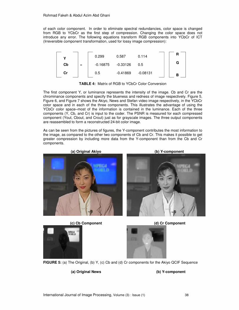
of each color component. In order to eliminate spectral redundancies, color space is changed from RGB to YCbCr as the first step of compression. Changing the color space does not introduce any error. The following equations transform RGB components into YCbCr of ICT (Irreversible component transformation, used for lossy image compression):
Y
0.299 0.587 0.114
R
Cb
=
-0.16875 -0.33126 0.5
G
Cr
0.5 -0.41869 -0.08131
B
TABLE 4: Matrix of RGB to YCbCr Color Conversion
The first component Y, or luminance represents the intensity of the image. Cb and Cr are the chrominance components and specify the blueness and redness of image respectively. Figure 5, Figure 6, and Figure 7 shows the Akiyo, News and Stefan video image respectively, in the YCbCr color space and in each of the three components. This illustrates the advantage of using the YCbCr color space–most of the information is contained in the luminance. Each of the three components (Y, Cb, and Cr) is input to the coder. The PSNR is measured for each compressed component (Yout, Cbout, and Crout) just as for grayscale images. The three output components are reassembled to form a reconstructed 24-bit color image. As can be seen from the pictures of figures, the Y-component contributes the most information to the image, as compared to the other two components of Cb and Cr. This makes it possible to get greater compression by including more data from the Y-component than from the Cb and Cr components.
(a) Original Akiyo (b) Y-component
(c) Cb Component (d) Cr Component
FIGURE 5: (a) The Original, (b) Y, (c) Cb and (d) Cr components for the Akiyo QCIF Sequence
(a) Original News (b) Y-component

Rohmad Fakeh & Abdul Azim Abd Ghani
International Journal of Image Processing, Volume (3) : Issue (1) 39
(c) Cb Component (d) Cr Component
FIGURE 6: a) The Original, (b) Y, (c) Cb and (d) Cr components for the News CIF Sequence
(a) Original Stefan (b) Y-component
(c) Cb Component (d) Cr Component
FIGURE 7: a) The Original, (b) Y, (c) Cb and (d) Cr components for the the Stefan SIF Sequence

Rohmad Fakeh & Abdul Azim Abd Ghani
International Journal of Image Processing, Volume (3) : Issue (1) 40
3.2 Wavelet Transformation Video compression techniques, which only remove spatial redundancy, cannot be highly effective. To achieve higher compression ratios the similarity of successive video frames has to be exploited. A) Temporal Compression The color source video sequences in QCIF, SIF and CIF formats are used producing sequences in Y, U and V color components as the input to the compression scheme. The average and difference between frames producing two temporal low-pass and high-pass sub-bands are calculated. For example the average and difference frame and the corresponding histogram plot for the 1
st. frame of Akiyo video sequence is given as in Figure 8.
Average Frame Hist(L_By)
Difference Frame Hist(H_By)
FIGURE 8: Wavelet decomposition of Average and Difference frame and the corresponding histogram plot for the 1
st. frame of Akiyo video sequence
B) Spatial Compression
For the application of the wavelet transform to images, cascaded 1D filters are used. The 1D discrete wavelet transformation step is calculated by using Mallat's pyramid algorithm [23]. First, the forward transformation combined with a down-sampling process of the image is performed, once in the horizontal and twice in the vertical direction. This procedure produces one low- and three high pass components. This procedure is applied recursively to the low pass output until the resulting low pass component reaches a size small enough to achieve effective compression of the image. In general, additional levels of transformation result in a higher compression ratio.
Spatial compression attempts to eliminate as much redundancy from single video frames as possible without introducing degradation of quality. This is done by first transforming the image from spatial to frequency domain and secondly by applying quantizing threshold the transformed coefficients. A two dimensional discrete wavelet transformation (DWT) is applied spatially to the images producing one level of decomposition into LL, LH, HL and HH sub-bands as in Figure 9. Figure 10 shows the High-pass and Low pass sub-bands with the low-pass sub-bands further decomposed and iterated. Figure 11 further illustrated the decomposition steps up to level three.

Rohmad Fakeh & Abdul Azim Abd Ghani
International Journal of Image Processing, Volume (3) : Issue (1) 41
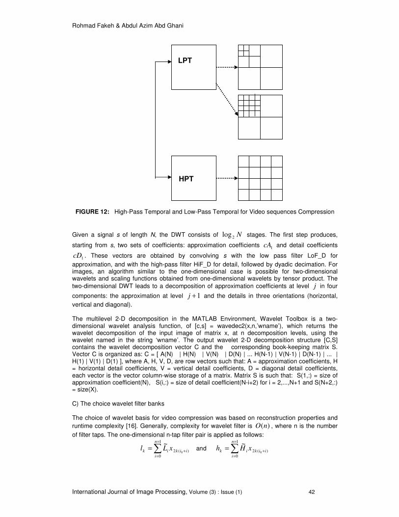
Both the Low-Pass-temporal and the High-Pass-Temporal sequences are shown to be spatially decomposed into a number of sub bands as in Figure 12.
FIGURE 9: Level one of 2-D DWT applied on an image
Highpass
f
Lowpass
FIGURE 10: Level one of 2-D DWT of Highpas and Lowpass
1-level 2-level 3-level
FIGURE 11: Level Three Dyadic DWT scheme used for Image Compression
IMAGE
LL
HL
HH
LH
G
H
H
G
H
G
IMAGE
LL HL
HH LH LH HH
HL
LH HH
HL
H
L
Rohmad Fakeh & Abdul Azim Abd Ghani
International Journal of Image Processing, Volume (3) : Issue (1) 42
FIGURE 12: High-Pass Temporal and Low-Pass Temporal for Video sequences Compression
Given a signal s of length N, the DWT consists of N2log stages. The first step produces,
starting from s, two sets of coefficients: approximation coefficients 1cA and detail coefficients
1cD . These vectors are obtained by convolving s with the low pass filter LoF_D for
approximation, and with the high-pass filter HiF_D for detail, followed by dyadic decimation. For images, an algorithm similar to the one-dimensional case is possible for two-dimensional wavelets and scaling functions obtained from one-dimensional wavelets by tensor product. The
two-dimensional DWT leads to a decomposition of approximation coefficients at level j in four
components: the approximation at level 1+j and the details in three orientations (horizontal,
vertical and diagonal). The multilevel 2-D decomposition in the MATLAB Environment, Wavelet Toolbox is a two-dimensional wavelet analysis function, of [c,s] = wavedec2(x,n,’wname’), which returns the wavelet decomposition of the input image of matrix x, at n decomposition levels, using the wavelet named in the string ‘wname’. The output wavelet 2-D decomposition structure [C,S] contains the wavelet decomposition vector C and the corresponding book-keeping matrix S. Vector C is organized as: C = [ A(N) | H(N) | V(N) | D(N) | ... H(N-1) | V(N-1) | D(N-1) | ... | H(1) | V(1) | D(1) ], where A, H, V, D, are row vectors such that: A = approximation coefficients, H = horizontal detail coefficients, V = vertical detail coefficients, D = diagonal detail coefficients, each vector is the vector column-wise storage of a matrix. Matrix S is such that: S(1,:) = size of approximation coefficient(N), S(i,:) = size of detail coefficient(N-i+2) for i = 2,...,N+1 and S(N+2,:) = size(X). C) The choice wavelet filter banks The choice of wavelet basis for video compression was based on reconstruction properties and
runtime complexity [16]. Generally, complexity for wavelet filter is )(nO , where n is the number
of filter taps. The one-dimensional n-tap filter pair is applied as follows:
∑=
=
+=
1
0
)(2 0
~n
i
iikik xLl and ∑=
=
+=
1
0
)(2 0
~n
i
iikik xHh
LPT
HPT

Rohmad Fakeh & Abdul Azim Abd Ghani
International Journal of Image Processing, Volume (3) : Issue (1) 43
L~
and H~
are the low- and high-pass filters, x the pixel values with row- or column-index i , and
k is the index of filter output. Iterating with step k2 automatically introduces the desired down-
sampling by 2. Filter coefficients are real numbers in the range [-1,1]. Much research effort has been expended in the area of wavelet compression, with the results indicating that wavelet approaches outperform DCT-based techniques [3], [4], [21], [25]. However, it is not completely clear which wavelets are suitable for video compression. Wavelets implemented using linear-phase filters are generally advantageous for image processing because such filters preserve the location of spatial details. A key component of an efficient video coding algorithm is motion compensation. However at the present time it is too computationally intensive to be used in software video compression. A number of low end applications therefore use motion-JPEG, in essence frame by frame transmission of JPEG images [29] with no removal of inter-frame redundancy. The choice of filter bank in wavelet image and video compression is a crucial issue that affects both image and video quality and compression ratio. A series of bi-orthogonal, and orthogonal wavelet filters of differing length were evaluated by compressing and decompressing a number of standard video test sequences, using different quantization thresholds. In this section, the selection of wavelet filter-banks of QCIF, CIF and SIF video sequences and their implications for the decoded image are discussed. A pool of color video sequences has been wavelet -transformed with different settings of the wavelet filter bank, boundary selection, quantization threshold and decomposition method. The reconstructed video sequences of QCIF sizes are evaluated using an objective quality of peak signal to noise ratio (PSNR). This section investigates how wavelet filter banks affect the subsequent quality and size of the reconstructed data, using a wavelet based video codec developed. Test video sequences were compressed with the codec, and the results obtained indicate that the choice of wavelet greatly influences the quality of the compressed data and its size. D) The Wavelet Filter-Banks The DWT is implemented using a two-channel perfect reconstruction linear phase filter bank [26]. Symmetric extension techniques are used to apply the filters near the frame boundaries; an approach that allows transforming images with arbitrary dimensions.
Rohmad Fakeh & Abdul Azim Abd Ghani
International Journal of Image Processing, Volume (3) : Issue (1) 44
3.3 Wavelet Threshold Selection This section describes wavelet thresholding for image compression under the framework provided by Statistical Learning Theory aka Vapnik-Chervonenkis (VC) theory. Under the framework of VC-theory, wavelet thresholding amounts to ordering of wavelet coefficients according to their relevance to accurate function estimation, followed by discarding insignificant coefficients. Existing wavelet thresholding methods specify an ordering based on the coefficient magnitude, and use threshold(s) derived under gaussian noise assumption and asymptotic settings. In contrast, the proposed approach uses orderings better reflecting statistical properties of natural images, and VC-based thresholding developed for finite sample settings under very general noise assumptions.
The plot of wavelet coefficients in Figure 4: (d) Frequency response after level 5 decomposition of Lena image in wavelet domain, suggests that small coefficients are dominated by noise, while coefficients with a large absolute value carry more signal information than noise. Stated more precisely, the motivation to this thresholding idea based on the following assumptions:
• The de-correlating property of a wavelet transform creates a sparce signal: most untouched coefficients are zero or close to zero.
• The noise level is not too high so that the signal wavelet coefficients can be distinguished from the noisy ones.
As it turns out, this method is indeed effective and thresholding is a simple and efficient method for noise reduction. A) Global thresholding Wavelet thresholding for image denoising involves taking the wavelet transform of an image (i.e., calculating the wavelet coefficients discarding setting to zero) the coefficients with relatively small or insignificant magnitudes. By discarding small coefficients one actually discard wavelet basis functions which have coefficients below a certain threshold. The denoised signal is obtained via inverse wavelet transform of the kept coefficients. One global threshold derived by Donoho [13], [14], [15] under gaussian noise assumption. Clearly, wavelet thresholding can be viewed a special case of signal/data estimation from noisy samples, which can be addressed within the framework of VC-theory. The original wavelet thresholding technique is equivalent to specifying a structure that uses only a magnitude ordering of the wavelet coefficients. Obviously, this is not the best way of ordering the coefficients. B) Level dependent threshold Level-dependent thresholding has been proposed to improve the performance of wavelet thresholding method. Instead of using a global threshold, level-dependent thresholding uses a group of thresholds, one for each scale level. It can be interpreted as the ordering of the wavelet coefficients with respect to their magnitudes adjusted by scale level. This suggests that the level-dependent thresholding be viewed as a special case of more sophisticated importance ordering in model selection based denoising method. A number of different structures (ordering schemes) can be specified on the same set of basis functions. A good ordering should reflect the prior knowledge about the signal/data being estimated. Similarly, 2-D image signal estimation with VC approach may require more complicated ordering scheme.
4. PERFORMANCE MEASURES Although there are several metrics that tend to be indicative of image quality, each of them has situations in which it fails to coincide with an observer's opinion [26]. However, since running human trials is generally prohibitively expensive, a number of metrics are often computed to help judge image quality. Some of the more commonly used "quality" metrics are given below,
),( nmx stands for the original data sized M by N, and ),( nmx)
the reconstructed mage.

Rohmad Fakeh & Abdul Azim Abd Ghani
International Journal of Image Processing, Volume (3) : Issue (1) 45
• MAE (Mean Absolute Error) MAE: One quantity, often computed in conjunction with other metrics, is maximum absolute error. Since this metrics measure error, it is regarded as inversely proportional to image quality.
MAE = Max | |),(),( nmxnmx)
− (1)
• MSE (Mean Square Error) MSE, RMS: Two other quantities that appear frequently when comparing original and reconstructed or approximated data are mean square error, and root mean square. These metrics attempt to measure an inverse to image quality.
MSE = [ ]∑∑−
=
−
=
−1
0
21
0
|),(),(.
1 M
j
N
i
nmxnmxMN
) (2)
RMS = MSE (3)
• SNR: Signal to noise ratio
SNR = 10 10log
[ ]
−∑∑
∑∑−
=
=
=
−
=
−
=
1
1
1
0
2
1
0
21
0
),(),(
),(
N
i
M
j
M
j
N
i
nmxnmx
nmx
) (4)
• Peak Signal-to-Noise Ratio (PSNR) Peak signal-to-noise ratio (PSNR) is the standard method for quantitatively comparing a compressed image with the original. For an 8-bit grayscale image, the peak signal value is 255. Hence the PSNR of an M×N 8-bit grayscale image x and its reconstruction ˆx is calculated. PSNR: Peak signal-to-noise ratio. The MSE and PSNR are directly related, and one normally uses PSNR to measure the coder's objective performance.
PSNR = 10 10log
MSE
2255 (5)
At high rate, images with PSNR above 32 dB are considered to be perceptually lossless. At medium and low rates, the PSNR does not agree with the quality of the image. For color images, the reconstruction of all three color spaces must be considered in the PSNR calculation. The MSE is calculated for the reconstruction of each color space. The average of these three MSEs is used to generate the PSNR of the reconstructed RGB image (as compared to the original 24-bit RGB image).
PSNR = 10 10log
RGBMSE
2255 (6)
Where RGBMSE is:-
RGBMSE = 3
gluegreenred MSEMSEMSE ++
(7)

Rohmad Fakeh & Abdul Azim Abd Ghani
International Journal of Image Processing, Volume (3) : Issue (1) 46
• Compression ratio (CR) Compression ratio is the relation between the amount of data of the original signal compared to the amount of data of the encoded signal [8]:
=CR)(
)(
encodeddataofAmount
signaloriginaldataofAmount (8)
5. RESULTS OF DECOMPOSITION STRATEGY To evaluate the decomposition strategy, three types of video sequences in QCIF resolutions with varying types of motion such as Miss America, Foreman and Carphone are used in the simulation. To compare the performance of the decomposition strategy between the dyadic discrete wavelet transform (DWT) and wavelet packet (WP), an empirical evaluation is conducted using three test video sequences of Miss America, Foreman and Carphone. Nine types of wavelet filter-banks s are used for the evaluation. They are Bior-22, Bior-2.6, Bior-4.4, Bior-6.8, Coif-2, Coif-3, Sym-4, Sym-5 and Sym-7. Global threshold is used in this evaluation, with values of threshold (thr) ranging from 10 to 125. For every filter-bank used for decoding the three video sequences, the average PSNR values for both the DWT and WP are calculated and tabulated as in Table 5 to Table 10. The corresponding plots of PSNR values Vs the filter-banks used are as in Figure 13 to Figure 18.
Thr=10
Miss America
Foreman
Carphone
Average PSNR [dB]
Filter Name
DWT WP DWT WP DWT WP DWT WP
Bior-2.2
Bior-2.6
Bior-4.4
Bior-6.8
Coif-2
Coif-3
Sym-4
Sym-5
Sym-7
42.09
42.40
41.80
41.96
41.97
41.89
41.98
42.03
41.86
40.90
40.88
40.73
40.86
30.33
40.06
30.02
41.86
39.96
38.16
38.34
38.28
38.33
38.42
38.39
38.41
38.39
38.34
32.85
32.78
33.38
33.33
21.99
30.18
22.36
36.10
28.47
39.99
40.18
39.71
39.63
39.87
39.74
39.88
39.85
39.62
33.77
33.18
34.37
34.07
22.30
31.47
21.34
37.86
29.90
40.08
40.31
39.93
39.98
40.08
40.01
40.09
40.09
39.94
35.84
35.61
36.16
36.09
24.88
33.90
24.57
38.60
32.78
TABLE 5: Average in PSNR for Wavelet Packet and Discrete Wavelet Transform of three video
sequences of Miss America, Foreman, and Carphone , using the best nine types filters and Global threshold of 10

Rohmad Fakeh & Abdul Azim Abd Ghani
International Journal of Image Processing, Volume (3) : Issue (1) 47
FIGURE 13: The Plot for Average PSNR for Wavelet Packet and Discrete Wavelet Transform of
using the best nine types of wavelet filters and Global threshold of 10
Thr=20
Miss America
Foreman
Carphone
Average PSNR [dB]
Filter Name
DWT WP DWT WP DWT WP DWT WP
bior-2.2
bior-2.6
bior-4.4
bior-6.8
coif-2
coif-3
sym-4
sym-5
sym-7
38.32
38.69
37.74
38.02
38.09
38.06
37.97
38.04
37.94
37.99
38.17
37.47
37.73
30.60
37.59
30.77
38.09
37.09
33.45
33.69
33.32
33.47
33.46
33.43
33.48
33.44
38.34
30.98
31.08
31.54
31.60
23.03
29.94
23.61
32.88
29.59
35.32
35.47
34.85
34.88
34.97
34.86
35.00
34.76
34.61
32.28
32.07
32.78
32.73
22.61
31.28
22.79
34.31
30.11
35.70
35.95
35.30
35.45
35.51
35.45
35.48
35.42
36.96
33.75
33.77
33.93
34.02
25.42
32.94
25.72
35.09
32.27
Table 6: Average in PSNR for Wavelet Packet and Discrete Wavelet Transform of three video
sequences of Miss America, Foreman, and Carphone, using the best nine types filters and Global threshold of 20

Rohmad Fakeh & Abdul Azim Abd Ghani
International Journal of Image Processing, Volume (3) : Issue (1) 48
FIGURE 14: The Plot for Average PSNR for Wavelet Packet and Discrete Wavelet Transform of using the best nine types of wavelet filters and Global threshold of 20
Thr=45
Miss America
Foreman
Carphone
Average PSNR [dB]
Filter Name
DWT WP DWT WP DWT WP DWT WP
bior-2.2
bior-2.6
bior-4.4
bior-6.8
coif-2
coif-3
sym-4
sym-5
sym-7
34.70
35.06
33.92
34.23
34.24
34.22
34.06
33.90
34.07
34.34
34.69
33.86
34.18
31.72
34.04
31.75
33.97
33.94
29.09
29.37
28.43
28.66
28.50
28.48
28.44
28.51
28.45
28.07
28.26
28.01
28.32
24.06
27.30
25.08
28.67
28.69
29.67
30.02
29.20
29.28
29.38
29.10
29.34
29.44
29.10
28.99
28.99
29.14
29.22
27.83
29.18
26.99
29.76
28.70
31.15
31.48
30.52
30.72
30.70
30.60
30.61
30.62
30.54
30.47
30.64
30.34
30.57
27.87
30.17
27.94
30.80
30.44
TABLE 7: Average in PSNR for Wavelet Packet and Discrete Wavelet Transform of three video sequences of Miss America, Foreman, and Carphone , using the best nine types
filters and Global threshold of 45
Rohmad Fakeh & Abdul Azim Abd Ghani
International Journal of Image Processing, Volume (3) : Issue (1) 49
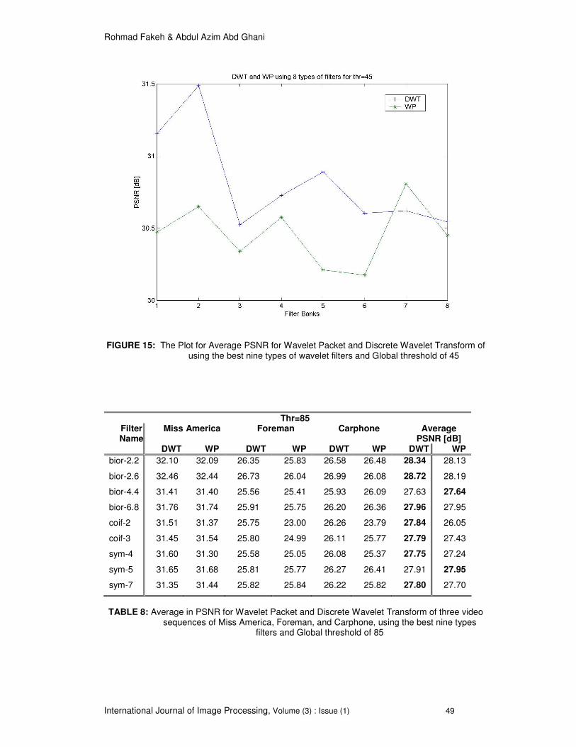
FIGURE 15: The Plot for Average PSNR for Wavelet Packet and Discrete Wavelet Transform of using the best nine types of wavelet filters and Global threshold of 45
Thr=85 Miss America
Foreman
Carphone
Average
PSNR [dB] Filter Name
DWT WP DWT WP DWT WP DWT WP
bior-2.2
bior-2.6
bior-4.4
bior-6.8
coif-2
coif-3
sym-4
sym-5
sym-7
32.10
32.46
31.41
31.76
31.51
31.45
31.60
31.65
31.35
32.09
32.44
31.40
31.74
31.37
31.54
31.30
31.68
31.44
26.35
26.73
25.56
25.91
25.75
25.80
25.58
25.81
25.82
25.83
26.04
25.41
25.75
23.00
24.99
25.05
25.77
25.84
26.58
26.99
25.93
26.20
26.26
26.11
26.08
26.27
26.22
26.48
26.08
26.09
26.36
23.79
25.77
25.37
26.41
25.82
28.34
28.72
27.63
27.96
27.84
27.79
27.75
27.91
27.80
28.13
28.19
27.64
27.95
26.05
27.43
27.24
27.95
27.70
TABLE 8: Average in PSNR for Wavelet Packet and Discrete Wavelet Transform of three video
sequences of Miss America, Foreman, and Carphone, using the best nine types filters and Global threshold of 85

Rohmad Fakeh & Abdul Azim Abd Ghani
International Journal of Image Processing, Volume (3) : Issue (1) 50
FIGURE 16: The Plot for Average PSNR for Wavelet Packet and Discrete Wavelet Transform of
using the best nine types of wavelet filters and Global threshold of 85
Thr=125 Miss America
Foreman
Carphone
Average
PSNR [dB] Filter Name
DWT WP DWT WP DWT WP DWT WP
bior-2.2
bior-2.6
bior-4.4
bior-6.8
coif-2
coif-3
sym-4
sym-5
sym-7
30.95
31.34
30.15
30.40
30.31
30.36
30.34
30.62
30.40
30.85
31.30
30.38
30.65
30.29
30.40
30.40
30.69
30.47
24.71
25.04
23.86
24.17
24.15
24.19
24.08
24.04
24.07
24.48
24.83
23.87
24.20
22.01
23.89
24.09
24.26
24.34
24.58
24.91
23.91
24.13
24.42
24.27
24.18
24.55
24.39
24.48
24.82
24.26
24.27
23.05
24.54
24.56
24.72
24.70
26.75
27.10
25.98
26.24
26.30
26.27
26.20
26.40
26.29
26.60
26.98
26.17
26.37
25.12
26.28
26.35
26.56
26.50
TABLE 9: Average in PSNR for Wavelet Packet and Discrete Wavelet Transform of three video
sequences of Miss America, Foreman and Carphone, using the best nine types of filters and Global threshold of 125

Rohmad Fakeh & Abdul Azim Abd Ghani
International Journal of Image Processing, Volume (3) : Issue (1) 51
FIGURE 17: The Plot for Average PSNR for Wavelet Packet and Discrete Wavelet Transform of using the best nine types of wavelet filters and Global threshold of 125
No. Video Sequences (WP) dB (DWT) dB Difference
(WP-DWT) - dB
1 Miss America 38.09 38.03 0.05
2 Suzie 34.59 34.58 0.01
3 Claire 37.21 37.26 -0.05
4 Mother & Daughter 33.77 33.69 0.07
5 Grandma 33.86 33.80 0.05
6 Carphone 34.88 34.53 0.34
7 Foreman 33.22 33.02 0.19
8 Salesman 32.38 32.19 0.18
TABLE 10: Average and difference in PSNR for Wavelet Packet and Discrete Wavelet Transform
of eight video sequences, using Sym5 Filter for Low-Pass-Temporal and Haar Filter for High-Pass-Temporal Frequencies, at two Decomposition Levels, and Global
threshold of 20
6. DISCUSSION The choice of decomposition strategy between dyadic transformation of Discrete Wavelet Transform (DWT) and Wavelet Packet (WP) Transform has been examined and found that DWT decomposition is preferred over the WP due to the superior values of PSNR generated throughout the simulations for all the lower values of global threshold from thr=10 and thr=20. For thr=45, wavelet filter of sym-5 resulted the WP outperforms DWT, and further for thr=85 and thr=125. At thr=85, bior-4.4 and sym-5 resulted the WP to outperform DWT. Only for higher value

Rohmad Fakeh & Abdul Azim Abd Ghani
International Journal of Image Processing, Volume (3) : Issue (1) 52
of global threshold of 125, the WP shows better PSNR values compared to DWT. However for the results of Table 10, the average difference of WP and DWT is only marginal when global threshold value of 20 and wavelet filter bank of sym-5 is used.
7. CONCLUSION This paper has addressed a number of challenges identified in 3D video compression based on wavelet transformation technique. The challenges appear when having to develop the coding scheme of 3D wavelet video coding, the question arises whether to transform the inter-frame followed by spatial filtering or vice versa. The substantial contribution on 3D wavelet coding is utilizing the spatio-temporal t-2D scheme, which has successfully exploited the wavelet transform technology and the best parameter strategies produces video output of high performance evaluated objectively using PSNR. It has shown that the selection of the parameters within the wavelet transform of periodic symmetric extension as the border distortion strategy, dyadic DWT, and level dependent thresholds have resulted to produce resulted in superior quality of the decoded video sequences. These parameters has been identified and further used in the proposed wavelet video compression (WVC) for the overall objective performance of the decoded video sequences. The spatio-temporal inter-frame temporal analysis of video sequences has been extended using Birge-Massaart strategy of wavelet shrinkage employing level-dependent quantization threshold. The objective evaluation pointed out that the PSNR values correlates better to different types of motion of the test video sequences especially to the Carphone sequence and using newly found Sym-5 filter-bank.
8. REFERENCES 1. Adami, N., Michele, B., Leonardi, R., and Signoroni, A. “A fully scalable wavelet video coding
scheme with homologous inter-scale prediction”. ST Journal of Research, 3(2):19-35, 2006
2. Adelson, E. H., and Simoncelli, E. “Orthogonal pyramid transforms for image coding”. In Proceedings of SPIE Visual Communications and Image Processing II, 845:50-58, 1987
3. Albanesi, M. G., Lotto, I., and Carrioli, L. “Image compression by the wavelet decomposition”. European Transactions on Telecommunication, 3(3):265-274, 1992.
4. Antonini, M., Barlaud, M., Mathieu, P., and Daubechies, I. “Image coding using wavelet transform”. IEEE Transactions on Image Processing, 1(2):205-220, 1992
5. Antonio, N. “Advances in Video Coding for hand-held device implementation in networked electronic media”. Journal of Real-Time Image Processing, 1:9-23, 2006
6. Ashourian, M.; Yusof, Z.M.; Salleh, S.H.S.; Bakar, S.A.R.A. “Robust 3-D subband video
coder”. Sixth International,Symposium on Signal Processing and its Applications, Vol 2:549–552, 2001
7. Brislawn, M. “Classification of non-expansive symmetric extension transforms for multirate filter banks”. Applied and Computational Harmonic Analysis, 3(4): 337-357,1996.
8. Claudia, S. “Decomposition strategies for wavelet-based image coding”. IEEE International Symposium on Signal Processing and its Applications (ISSPA), Vol. 2: 529-532, Kuala Lumpur, Malaysia, 2001.
9. Daubechies, I. “Orthonormal bases of compactly supported wavelets". Commun. Pure Applied. Math, 41:909-996, 1988.
10. Daubechies, I. “The wavelet transform, time-frequency localization and signal analysis”. IEEE Trans. on Information Theory, 36(5):961-1005, 1990.
11. Daubechies, I. “Ten Lectures on Wavelets”. Philadelphia, Pennsylvania: Society for Industrial and Applied Mathematics (SIAM), 1992

Rohmad Fakeh & Abdul Azim Abd Ghani
International Journal of Image Processing, Volume (3) : Issue (1) 53
12. Daubechies, I. and Sweldens, W. “Factoring wavelet transforms into lifting steps”. Journal of Fourier Analysis and Applications, 4(3):245-267, 1998.
13. Donoho, L. “De-noising by soft-thresholding”. IEEE Transactions on Information Theory, 41(3):613-627, 1995.
14. Donoho, L. and Johnstone, I. M. “Ideal spatial adaptation via wavelet shrinkage”. Biometrika, 81(3):425-455, 1994.
15. Donoho, L. and Johnstone, I. M. “Minimax estimation via wavelet shrinkage”. The Annals of Statistics, 26(3):879-921, 1998.
16. George, F., Dasen, M., Weiler, N., Plattner, B., and Stiller, B. “The wavevideo system and network architecture: design and implementation”. Technical report No. 44. Computer Engineering & Networks Laboratory (TIK), E7H, Zurich, Switzerland, 1998.
17. Golwelkar, A. V. and Woods, J. W. “Scalable video compression using longer motion-compensated temporal filters”. VCIP 2003: 1406-1416, 2003
18. Hsiang, S. T. and Woods, J. W. “Embedded video coding using invertible motion
compensated 3-D subband/wavelet filter bank”. Journal of Signal Processing: Image Communication, Vol. 16: 705-724, 2001.
19. Karlsson, G. and Vetterli, M. “Three dimensional subband coding of video”.In Proceedings of
IEEE Int. Conf. Acoustics, Speech, and Signal Processing (ICASSP), II:1100-1103, 1988. 20. Lewis, A. S. and Knowles, G. “Video compression using 3D wavelet transforms”. Electronic
Letters, 26(6):396-398, 1990.
21. Lewis, A. S. and Knowles, G. “Image compression using the 2-D wavelet transform”. IEEE Trans. Image Processing, 1:244-250, 1992.
22. Luo, J. “Low bit rater wavelet-based image and video compression with adaptive quantization, coding and post processing”. Technical Report EE-95-21. The University of Rochester, School of Engineering and Applied Science, Department of Electrical Engineering, Rochester, New York, 1995.
23. Mallat, S. G. 1989. “A theory for multiresolution signal decomposition: the wavelet representation”. IEEE Transactions on Pattern Analysis and Machine Intelligence, 11(7):674-693, 1989.
24. Podilchuk, Jayant, N. S., and Farvardin, N. “Three-dimensional subband coding of video”. IEEE Translation of Image Processing, 4(2): 125-139, 1995.
25. Shapiro, J. M. “Embedded image coding using zerotrees of wavelets coefficients”. IEEE Transactions on Signal Processing, 41(12):3445-3462, 1993.
26. Strang, G., and Nguyen, T. “Wavelets and Filter Banks”. Wellesley-Cambridge Press, Wellesley, MA, USA, 1997.
27. Taubman, D., and Zakhor, A. “Multirate 3-D subband coding of video”. IEEE Transactions on Image Processing, 3(5): 572-588, 1994
28. Vass, J., Zhuang, S., Yao, J., and Zhuang, X. “Mobile video communications in wireless environments”. In Proceedings of IEEE Workshop on Multimedia Signal Processing, Copenhagen, Denmark: 45-50, 1999
29. Wallace, G. K. “The JPEG still picture compression standard”. Comm. ACM, 34(4):30-44, 1994.
Rohmad Fakeh & Abdul Azim Abd Ghani
International Journal of Image Processing, Volume (3) : Issue (1) 54
30. Wang, X., and Blostern, S. D. 1995. “Three–dimensional subband video transmission through mobile satellite channels”. In Proceedings of International Conference on Image Processing, Vol. 3, pp. 384-387, 1995.