An Emission Inventory of Non-point Oil and Gas Emissions Sources in the Western Region

James Russell, Alison Pollack and Greg Yarwood

ENVIRON International Corporation, 101 Rowland Way, Novato, CA 94945 jrussell@environcorp.com

ABSTRACT

As part of an effort undertaken by the Western Regional Air Partnership (WRAP) to consolidate and improve on the 2002 state and tribal emission inventories, ENVIRON developed an emission inventory of non-point emission sources associated with the production of oil and gas. This inventory focused on emissions of nitrous oxides from compressor engines, drill rig engines and coalbed methane pump engines. Methodologies were developed that could be applied consistently across the western region, without overlooking the variability in local production characteristics, control requirements and inventory thresholds. Application of these methodologies resulted in the addition of almost 120,000 tons of NOx emissions to the 2002 WRAP emission inventory. New spatial surrogates were generated based on well locations to appropriately distribute these emissions.

An oil and gas inventory for 2018 was estimated by growing the 2002 inventory using growth factors derived from resource management plans produced by the Bureau of Land Management and regional forecasts made by the Energy Information Administration. Additional effort was made to estimate emissions in new development areas without base year emissions. The resulting approach incorporated the most complete information available on the anticipated oil and gas development in the western region to produce an inventory that predicts a doubling of non-point oil and gas NOx emissions between 2002 and 2018. A complementary project recently completed by the authors in Northeast Texas has demonstrated a control technology for compressor engines with the potential to eliminate approximately 80 percent of the 2002 to 2018 growth in NOx emissions at cost of less than $200 per ton. INTRODUCTION Background

In 2002, more than 8.3 trillion cubic feet of natural gas and 820 million barrels of crude oil were drawn from oil and gas wells in the 14 western states1,2. To achieve this level of production, an extensive fleet of oil and gas production equipment operates continuously across the region. The sizes and types of equipment in that fleet vary from small chemical injection pumps up to gas turbines of several thousand horsepower. Despite their differences, at least one common feature unites many of these equipment types. They emit nitrous oxides (NOx), volatile organic compounds (VOC) and other air pollutants as part of their normal daily operations. Even the smallest of these source types may result in significant emissions when the continuous operation and the number of units are taken into consideration.

Previous emission inventories have addressed limited segments of the oil and gas production industry. In particular, large oil and gas facilities have been well accounted for in state point source inventories. Attempts have also been made to capture some of the smaller oil and gas sources in area source inventories. The 2002 emission inventories prepared by the State of Wyoming and the State of California include emissions for a number of smaller wellhead processes. Additional studies have made gains in characterizing oil and gas emissions in major development areas, such as the San Juan Basin and Jonah-Pinedale. These studies advanced the understanding of emissions from this industry, but the

magnitude of emissions they uncovered also highlighted the absence of area source oil and gas emissions in the inventories of other states and production areas. Objective and Approach

The methodologies and results presented in this paper are the synthesis of three separate studies to characterize emissions from the oil and gas production industry and to determine if future reductions of these emissions could make a significant contribution toward improved air quality. These three studies were as follows:

• 2002 and 2018 state oil and gas inventories prepared for the Stationary Sources Joint Forum (SSJF) of the Western Regional Air Partnership (WRAP) – The WRAP-SSJF commissioned this study to develop and implement an emission inventory methodology for oil and gas sources in the 14 member states – Alaska, Arizona, California, Colorado, Idaho, Montana, Nevada, North Dakota, Oregon, South Dakota, Utah, Washington and Wyoming. This inventory adopted the oil and gas point source emissions from the existing state inventories and reconciled new oil and gas area source inventories with those existing point source emissions. Discussion of this inventory is limited to the development of county level area source oil and gas emissions estimates.

• 2002 and 2018 tribal oil and gas inventories prepared for the Tribal Data Development

Work Group (TDDWG) of the WRAP – In this study, oil and gas emission inventories were prepared for three tribes – the Arapahoe and Shoshone of the Wind River Reservation, the Navajo Nation and the Ute Mountain Ute. Emissions estimates were prepared using the inventory methodology developed for the WRAP-SSJF project, with adjustments to utilize the activity data available for each tribe.

• Pilot project to evaluate the effectiveness of an emission control system for gas compressor

engines conducted for Northeast Texas Air Care (NETAC) – In 2004, NETAC commissioned a pilot project to demonstrate the effectiveness of available technology in reducing nitrogen oxide emissions from compressor engines used in gas production operations. This pilot project succeeded in retrofitting five gas compressor engines with controls that reduced NOx emissions from those engines by greater than 90 percent.

The discussion of these three projects in this paper is organized to focus on the major themes of the three studies – emission inventory development, future year emission projections and emission control strategies. As such, the development of the base year 2002 area source oil and gas inventories for the states and for the tribes is discussed in the first two sections of this paper. The third section describes the procedures used to project oil and gas emissions in the year 2018. This is followed by a brief discussion of the spatial allocation surrogates that were created to facilitate the modeling of those emissions. The final section then relates the results of the pilot project to evaluate an emission control technology for gas compressor engines. WRAP - STATE OIL AND GAS INVENTORIES

The objective of this study was to develop and implement a uniform procedure for estimating area source emissions from oil and gas production operations across the western region. The emphasis of this study was on estimating emissions of pollutants with the potential to impair visibility near Class I areas in the west, in particular NOx emissions. Drill rigs, compressor engines and coalbed methane (CBM) pump engines were focused on because of their importance as NOx sources and the anticipated growth in the use of these equipment types as oil and gas development continues in the region. In

addition, emissions were estimated for a number of sources collectively referred to as ‘minor NOx and VOC sources’ for which production-based emission factors had been developed. Drill Rig Emissions

The approach developed to estimate emissions from drill rig engines used drill permit data from

oil and gas commissions (OGCs) as a measure of activity and emission factors derived from a survey of drilling companies. The drill permit data found to be available from the state OGCs was as follows:

• Spud date - the date that drilling commenced • Well depth - the depth of the well; total vertical, measured or target depending on availability • Completion date - the date well preparation is finalized; occurring with some delay after drilling

ceases • Well formation - the geologic structure that the well was drilled to • Well field - the legal designation for the area where the well was drilled • Well county - the county where the well was drilled; for allocation purposes

The data maintained by state OGCs provided the base level of activity to characterize the number of wells being drilled in an area, the depth of those wells and the amount of time required to construct the wells. To translate that activity data to emissions estimates required the derivation of locally appropriate emission factors from a study of drilling emissions that was completed by the Wyoming Department of Environmental Quality3.

The information provided by WY DEQ represented the synthesis of emissions estimates made by ten different drilling companies for a total of 218 wells drilled. The WY DEQ study yielded emission factors of 13.5 tons NOx and 3.3 tons SO2 per well. However, because emissions from the drilling of a well are dependent upon the depth of the well, the composition of substrate and the characteristics of the rig engine(s), it was not appropriate to use the Jonah-Pinedale emission factors for all wells drilled in the WRAP States without some adjustment. We therefore developed a methodology that uses information about the characteristics of wells in a specific area to scale the Jonah-Pinedale emission factor to better represent drilling operations in that area.

The most local unit for which typical well characteristics were commonly available was the formation. To create emission factors for drilling in a given formation, it was necessary to make two important assumptions. First it was assumed that the difference between the completion date and the date that drilling ceased is, on average, constant relative to the total duration of well preparation activities. This assumption was needed because the actual date that drilling ceased was not available. It was also necessary to assume that the capacity of the equipment used to drill a well was dependent upon the depth of the well. This assumption was made because the data clearly indicated that substantially different rigs were employed in different drilling applications. With those two assumptions, it was possible to scale the emission factor from the Jonah-Pinedale area to other formations based on the average well depth and drilling duration and in doing so to correct for variations due to well depth, composition of substrate, and engine capacity.

The average well depth and drilling duration for the formations drilled in Jonah-Pinedale - based

on drill permit data obtained from the Wyoming OGC for 2002 and 2004 - was 11,896 ft and 80.6 days4. The same type of average well depth and drilling duration was calculated for the other formations drilled in 2002 in the WRAP States. A formation specific emission factor was then created for each formation using Calculation 1.

Calculation 1:

Additional adjustments were considered beyond those for well depths and durations. State DEQs were surveyed to determine the control requirements for drill rigs. All state DEQs responded that controls were not required on drill rig engines. An adjustment was, however, necessary to account for the varying fuel sulfur levels between different states and counties. This adjustment was accomplished by multiplying the county SO2 emission by the ratio of that county’s nonroad diesel sulfur level to the Wyoming nonroad diesel sulfur level. Emissions for each formation were calculated as the product of the formation specific emission factor and the number of wells drilled in the formation in 2002. The emissions for that formation were then allocated to the counties that intersected the formation based on the fraction of the wells drilled that were drilled in each county’s portion of the formation. The state total drill rig NOx and SO2 emissions that resulted from this procedure are shown in Table 1. The adjustments made to the emission factors are apparent in these results. While significantly more wells were drilled in the State of Wyoming than in New Mexico, the emissions in New Mexico are higher than in Wyoming. This occurs because many of the Wyoming wells were drilled quickly and to a shallow depth, as commonly occurs for the Powder River Basin CBM wells. In contrast, the wells in New Mexico were, on average, drilled deeper and took longer to drill. Where average drill depths and durations were more comparable, such as in Colorado and New Mexico, the emissions per well are relatively close. Table 1. State total drill rig emissions.

State Wells Drilled NOx (tons) SO2 (tons) Alaska 205 877 66 Arizona Colorado 1,244 5,734 260 Idaho Montana 463 1,044 227 Nevada 6 24 1 New Mexico 932 6,645 1,444 North Dakota 157 1,536 358 Oregon South Dakota 7 36 8 Utah 126 676 147 Washington Wyoming 2,948 4,964 1,213 Total 6,088 21,536 3,706

EFA = EFJ x ( DA / DJ) x ( TA / TJ )

where:

EFA = The emission factor for another formation EFJ = The Jonah-Pinedale emission factor DA = The average depth of wells drilled in another area Dj = The average depth of wells drilled in Jonah-Pinedale TA = The duration of drilling in another area

Tj = The duration of drilling in Jonah-Pinedale

Non-Point Natural Gas Compressor Engine Emissions

The focus of this area source compressor engine emission estimate was the group of relatively small, dispersed wellhead compressor engines. In all but two of the natural gas producing states, these engines had not been included in previous emission inventories and their inclusion here represents a significant advance in understanding this important component of the gas production industry.

To estimate emissions from compressor engines, a production-based emission factor was developed from a local study of compressor engine emissions. This emission factor was combined with gas production data collected from the state OCGs to estimate emissions. Several local studies were analyzed to determine which offered the most appropriate data from which to derive the emission factor. The strengths and weaknesses of each of those studies was evaluated, and ultimately, an industry-compiled inventory of wellhead compressor engines in the New Mexico portion of the San Juan Basin was selected.

The New Mexico Oil and Gas Association (NMOGA) cooperated in the preparation of the Denver Early Action Compact by compiling an inventory for year 2002 of the unpermitted emissions sources operated by the oil and gas production industry in the New Mexico portion of the San Juan Basin. The NMOGA inventory was based on a survey of exploration and production companies. The survey obtained responses representing activity at 10,582 of 17,108 wells. Emissions for wellhead compressor engines submitted by the responding companies totaled 14,892 tons NOx5. To estimate the emissions at all wells, this emission was divided by the fraction of wells represented in the responses. This produced an estimate of 24,076 tons of NOx emitted by wellhead compression in the New Mexico portion of the San Juan Basin.

This emission estimate corresponds to gas production in three New Mexico counties: Rio Arriba, San Juan and Sandoval. A total 2002 gas production of 1,030 BCF in those three counties was obtained from the online production database maintained by the New Mexico Institute of Mining and Technology6. With these estimates of total gas production and total emissions for wellhead compression, it was possible to calculate a production based emission factor as the quotient of total emissions divided by total gas production. The result is an emission factor of 2.3x10-5 tons NOx per MCF gas produced.

We had previously requested from the OGCs well-specific oil and gas production statistics. These were obtained, either submitted by the OGC or downloaded from the online production statistics maintained by some states OGCs, for all oil and gas producing states. For the compressor engine emissions estimate, total 2002 natural gas production was summed for each county and county level emissions were estimated as the product of natural gas production and the production-based emission factor.

The only states that reported requiring controls on compressor engines were Utah and Wyoming. In both of those states, the emissions are controlled to a rate of 1-2 grams NOx per hp-hr7,8. This represents a substantial reduction from the average emission rate of 11.4 grams NOx/hp-hr that was found by the NMOGA Inventory. In both Utah and Wyoming, the controlled emission factor was calculated as the product of the uncontrolled emission factor and the ratio of controlled hourly emissions to uncontrolled hourly emissions, 2 grams NOx/hp-hr to 11.4 grams NOx/hp-hr. The state total NOx emissions that resulted from the application of these emission factors are presented in Table 2. As is shown in Table 2, the emissions resulting from this procedure are directly related to production. Though at the level of individual wells it may be true that compressor activity is actually higher at less productive wells, when county level production is considered, as in this study, this positive correlation of compressor engine emissions to gas production is supported by all of the studies considered in the development of this methodology.

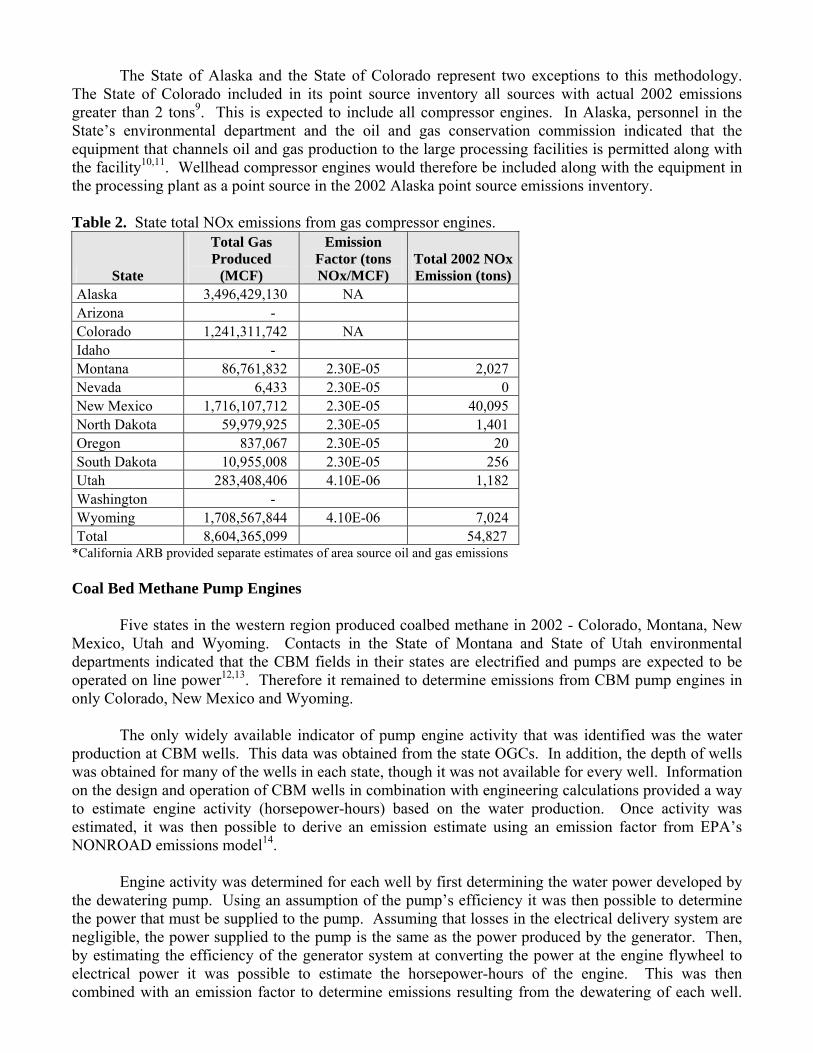
The State of Alaska and the State of Colorado represent two exceptions to this methodology.

The State of Colorado included in its point source inventory all sources with actual 2002 emissions greater than 2 tons9. This is expected to include all compressor engines. In Alaska, personnel in the State’s environmental department and the oil and gas conservation commission indicated that the equipment that channels oil and gas production to the large processing facilities is permitted along with the facility10,11. Wellhead compressor engines would therefore be included along with the equipment in the processing plant as a point source in the 2002 Alaska point source emissions inventory. Table 2. State total NOx emissions from gas compressor engines.

State

Total Gas Produced

(MCF)

Emission Factor (tons NOx/MCF)

Total 2002 NOx Emission (tons)

Alaska 3,496,429,130 NA Arizona - Colorado 1,241,311,742 NA Idaho - Montana 86,761,832 2.30E-05 2,027 Nevada 6,433 2.30E-05 0 New Mexico 1,716,107,712 2.30E-05 40,095 North Dakota 59,979,925 2.30E-05 1,401 Oregon 837,067 2.30E-05 20 South Dakota 10,955,008 2.30E-05 256 Utah 283,408,406 4.10E-06 1,182 Washington - Wyoming 1,708,567,844 4.10E-06 7,024 Total 8,604,365,099 54,827

*California ARB provided separate estimates of area source oil and gas emissions Coal Bed Methane Pump Engines

Five states in the western region produced coalbed methane in 2002 - Colorado, Montana, New

Mexico, Utah and Wyoming. Contacts in the State of Montana and State of Utah environmental departments indicated that the CBM fields in their states are electrified and pumps are expected to be operated on line power12,13. Therefore it remained to determine emissions from CBM pump engines in only Colorado, New Mexico and Wyoming.

The only widely available indicator of pump engine activity that was identified was the water production at CBM wells. This data was obtained from the state OGCs. In addition, the depth of wells was obtained for many of the wells in each state, though it was not available for every well. Information on the design and operation of CBM wells in combination with engineering calculations provided a way to estimate engine activity (horsepower-hours) based on the water production. Once activity was estimated, it was then possible to derive an emission estimate using an emission factor from EPA’s NONROAD emissions model14.

Engine activity was determined for each well by first determining the water power developed by the dewatering pump. Using an assumption of the pump’s efficiency it was then possible to determine the power that must be supplied to the pump. Assuming that losses in the electrical delivery system are negligible, the power supplied to the pump is the same as the power produced by the generator. Then, by estimating the efficiency of the generator system at converting the power at the engine flywheel to electrical power it was possible to estimate the horsepower-hours of the engine. This was then combined with an emission factor to determine emissions resulting from the dewatering of each well.

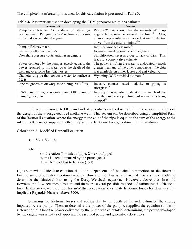
The complete list of assumptions used for this calculation is presented in Table 3. Table 3. Assumptions used in developing the CBM generator emissions estimate.

Assumption Reason Pumping in NM and CO is done by natural gas fired engines. Pumping in WY is done with a mix of natural gas and diesel engines.

WY DEQ data shows that the majority of pump engine horsepower is natural gas fired15. Also, industry representatives indicate that use of electric power from the grid is minimal16.

Pump efficiency = 0.6 Industry provided estimate17. Generator efficiency = 0.85 Estimate based on small size of engines. Downhole pressure contribution is negligible Simplification necessary due to lack of data. This

leads to a conservative estimate. Power delivered by the pump is exactly equal to the power required to lift water over the depth of the well and overcome frictional losses.

The power in lifting the water is undoubtedly much greater than any of the other components. No data was available on minor losses and exit velocity.

Diameter of pipe that conducts water to surface is 0.2 ft

Wyoming OGC provided estimate18

Pipe roughness of drawn/plastic tubing (5x10-6 ft) Industry contact stated majority of piping is fiberglass19

8760 hours of engine operation and 4380 hours of pumping per year

Industry representative indicated that much of the time the engine is operating, but no water is being pumped16.

Information from state OGC and industry contacts enabled us to define the relevant portions of

the design of the average coal bed methane well. This system can be described using a simplified form of the Bernoulli equation, where the energy at the exit of the pipe is equal to the sum of the energy at the inlet plus the energy supplied by the pump and the frictional losses, as shown in Calculation 2. Calculation 2. Modified Bernoulli equation

21 zHHz LP =++ where: z = Elevation (1 = inlet of pipe, 2 = exit of pipe)

Hp = The head imparted by the pump (feet) HL = The head lost to friction (feet)

HL is somewhat difficult to calculate due to the dependence of the calculation method on the flowrate. For the same pipe under a certain threshold flowrate, the flow is laminar and it is a simple matter to determine the frictional loss using the Darcy-Weisbach equation. However, above that threshold flowrate, the flow becomes turbulent and there are several possible methods of estimating the frictional loss. In this study, we used the Hazen-Williams equation to estimate frictional losses for flowrates that implied a Reynolds Number above 3000.

Summing the frictional losses and adding that to the depth of the well estimated the energy imparted by the pump. Then, to determine the power of the pump we applied the equation shown in Calculation 3. Once the power delivered by the pump was calculated, determining the power developed by the engine was a matter of applying the assumed pump and generator efficiencies.

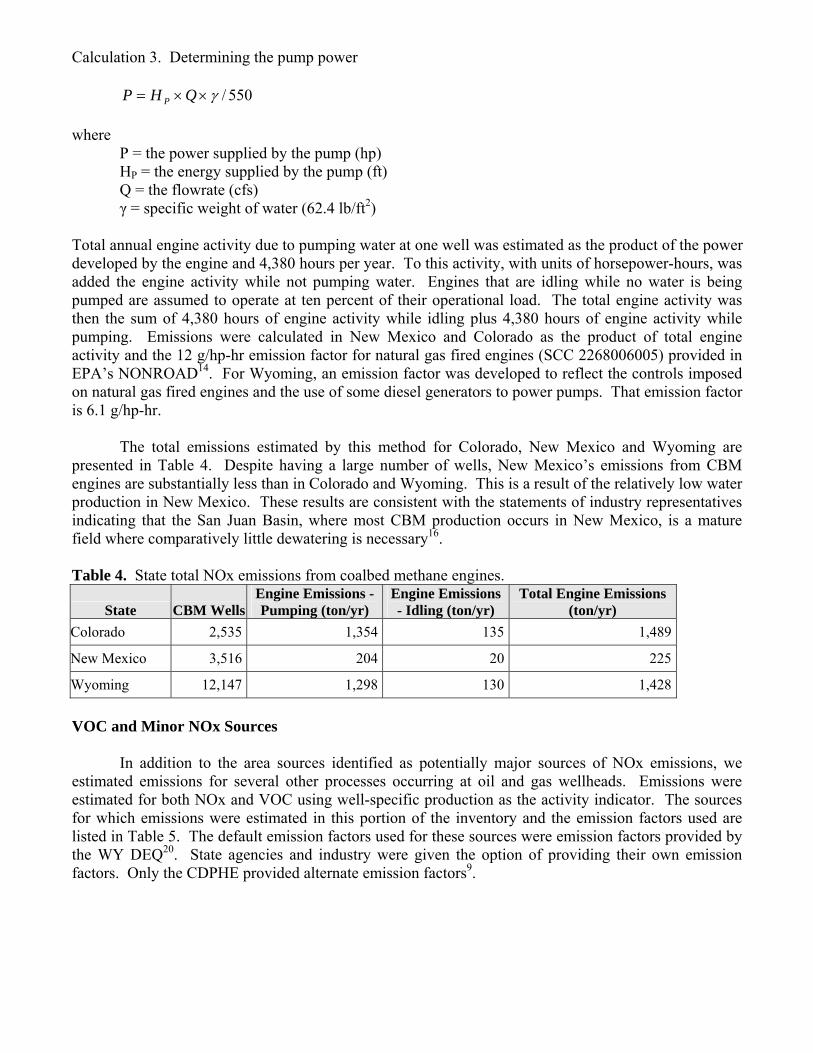
Calculation 3. Determining the pump power 550/γ××= QHP P where P = the power supplied by the pump (hp) HP = the energy supplied by the pump (ft) Q = the flowrate (cfs) γ = specific weight of water (62.4 lb/ft2) Total annual engine activity due to pumping water at one well was estimated as the product of the power developed by the engine and 4,380 hours per year. To this activity, with units of horsepower-hours, was added the engine activity while not pumping water. Engines that are idling while no water is being pumped are assumed to operate at ten percent of their operational load. The total engine activity was then the sum of 4,380 hours of engine activity while idling plus 4,380 hours of engine activity while pumping. Emissions were calculated in New Mexico and Colorado as the product of total engine activity and the 12 g/hp-hr emission factor for natural gas fired engines (SCC 2268006005) provided in EPA’s NONROAD14. For Wyoming, an emission factor was developed to reflect the controls imposed on natural gas fired engines and the use of some diesel generators to power pumps. That emission factor is 6.1 g/hp-hr.

The total emissions estimated by this method for Colorado, New Mexico and Wyoming are presented in Table 4. Despite having a large number of wells, New Mexico’s emissions from CBM engines are substantially less than in Colorado and Wyoming. This is a result of the relatively low water production in New Mexico. These results are consistent with the statements of industry representatives indicating that the San Juan Basin, where most CBM production occurs in New Mexico, is a mature field where comparatively little dewatering is necessary16. Table 4. State total NOx emissions from coalbed methane engines.

State CBM Wells Engine Emissions - Pumping (ton/yr)

Engine Emissions - Idling (ton/yr)

Total Engine Emissions (ton/yr)

Colorado 2,535 1,354 135 1,489

New Mexico 3,516 204 20 225

Wyoming 12,147 1,298 130 1,428 VOC and Minor NOx Sources

In addition to the area sources identified as potentially major sources of NOx emissions, we estimated emissions for several other processes occurring at oil and gas wellheads. Emissions were estimated for both NOx and VOC using well-specific production as the activity indicator. The sources for which emissions were estimated in this portion of the inventory and the emission factors used are listed in Table 5. The default emission factors used for these sources were emission factors provided by the WY DEQ20. State agencies and industry were given the option of providing their own emission factors. Only the CDPHE provided alternate emission factors9.

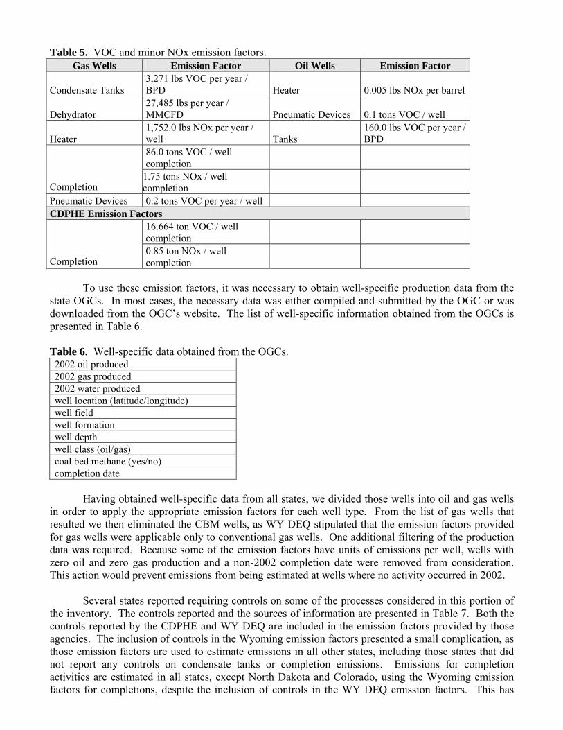
Table 5. VOC and minor NOx emission factors.

Gas Wells Emission Factor Oil Wells Emission Factor

Condensate Tanks 3,271 lbs VOC per year / BPD Heater 0.005 lbs NOx per barrel

Dehydrator 27,485 lbs per year / MMCFD Pneumatic Devices 0.1 tons VOC / well

Heater 1,752.0 lbs NOx per year / well Tanks

160.0 lbs VOC per year / BPD

86.0 tons VOC / well completion

Completion 1.75 tons NOx / well completion

Pneumatic Devices 0.2 tons VOC per year / well CDPHE Emission Factors

16.664 ton VOC / well completion

Completion 0.85 ton NOx / well completion

To use these emission factors, it was necessary to obtain well-specific production data from the

state OGCs. In most cases, the necessary data was either compiled and submitted by the OGC or was downloaded from the OGC’s website. The list of well-specific information obtained from the OGCs is presented in Table 6. Table 6. Well-specific data obtained from the OGCs. 2002 oil produced 2002 gas produced 2002 water produced well location (latitude/longitude) well field well formation well depth well class (oil/gas) coal bed methane (yes/no) completion date

Having obtained well-specific data from all states, we divided those wells into oil and gas wells

in order to apply the appropriate emission factors for each well type. From the list of gas wells that resulted we then eliminated the CBM wells, as WY DEQ stipulated that the emission factors provided for gas wells were applicable only to conventional gas wells. One additional filtering of the production data was required. Because some of the emission factors have units of emissions per well, wells with zero oil and zero gas production and a non-2002 completion date were removed from consideration. This action would prevent emissions from being estimated at wells where no activity occurred in 2002.

Several states reported requiring controls on some of the processes considered in this portion of the inventory. The controls reported and the sources of information are presented in Table 7. Both the controls reported by the CDPHE and WY DEQ are included in the emission factors provided by those agencies. The inclusion of controls in the Wyoming emission factors presented a small complication, as those emission factors are used to estimate emissions in all other states, including those states that did not report any controls on condensate tanks or completion emissions. Emissions for completion activities are estimated in all states, except North Dakota and Colorado, using the Wyoming emission factors for completions, despite the inclusion of controls in the WY DEQ emission factors. This has

been done because the flaring assumed in the emission factor is not very different from the flaring we would assume based only on safety considerations. Table 7. Controls on sources considered in the VOC and minor NOx source inventory.

State Condensate

Tanks Completion: Flaring &

Venting Source Colorado Included in EF provided CDPHE, 2005;

CDPHE, 2005b Montana Flare or vapor

recovery required

Flare or vapor recovery required

MT DEQ, 2005

North Dakota Flare or vapor recovery required

Flare or vapor recovery required

ND DH, 2005

Wyoming Included in EF provided

Included in EF provided WY DEQ, 2004b

WY DEQ assumed that condensate tanks with greater than 18.3 barrels per day of condensate

production would be controlled with an overall efficiency of 98 percent. For wells with condensate production less than 18.3 barrels per day WY DEQ provided an uncontrolled emission factor. Depending upon the specific control requirements in each state, the controlled and uncontrolled factors were applied to no wells, to some fraction of wells, or to all wells. Different control requirements were also applied to completion emissions across the region. A summary of the final, control-adjusted gas well emission factors used is presented in Table 8. The final oil well emission factors used are those presented in Table 5. These emission factors were combined with the well data to estimate emissions following the general procedure shown in Calculation 4. Table 8. Summary of control-adjusted gas well emission factors for VOC and minor NOx sources.

Gas Well Process

State

Condensate

Tanks (lb VOC per year/BPD)

Dehydrator

(lbs VOC per year/MCFD)

Heater (lbs

NOx per year/well)

Completion

(tons per completion)

Pneumatic Devices (tons

VOC per year/well)

Alaska NA NA VOC = 86 NOx = 1.75

Colorado NA NA 1,752 VOC = 16.7 NOx = 0.85 0.2

Montana 65 NA 1,752 VOC = 2.3 NOx = 3.5 0.2

North Dakota 65 27,485 1,752 VOC = 86 NOx = 1.75 0.2

All Other States 3,271 27,485 1,752 VOC = 86

NOx = 1.75 0.2

Wyoming 3,271

(uncontrolled) 65 (controlled)

27,485 1,752 VOC = 86 NOx = 1.75 0.2

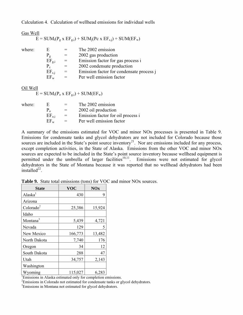
Calculation 4. Calculation of wellhead emissions for individual wells Gas Well

E = SUMi(Pg x EFg,i) + SUMj(Pc x EFc,j) + SUM(EFw) where: E = The 2002 emission

Pg = 2002 gas production EFg,i = Emission factor for gas process i Pc = 2002 condensate production EFc,j = Emission factor for condensate process j EFw = Per well emission factor

Oil Well

E = SUMi(Po x EFg,i) + SUM(EFw) where: E = The 2002 emission

Po = 2002 oil production EFo,i = Emission factor for oil process i EFw = Per well emission factor

A summary of the emissions estimated for VOC and minor NOx processes is presented in Table 9. Emissions for condensate tanks and glycol dehydrators are not included for Colorado because those sources are included in the State’s point source inventory21. Nor are emissions included for any process, except completion activities, in the State of Alaska. Emissions from the other VOC and minor NOx sources are expected to be included in the State’s point source inventory because wellhead equipment is permitted under the umbrella of larger facilities10,11. Emissions were not estimated for glycol dehydrators in the State of Montana because it was reported that no wellhead dehydrators had been installed22. Table 9. State total emissions (tons) for VOC and minor NOx sources.

State VOC NOx Alaska1 430 9Arizona Colorado2 25,386 15,924Idaho Montana3 5,439 4,721Nevada 129 5New Mexico 166,773 13,482North Dakota 7,740 176Oregon 34 12South Dakota 288 47Utah 34,757 2,143Washington Wyoming 115,027 6,283

1Emissions in Alaska estimated only for completion emissions. 2Emissions in Colorado not estimated for condensate tanks or glycol dehydrators. 3Emissions in Montana not estimated for glycol dehydrators.

WRAP - TRIBAL OIL AND GAS INVENTORIES

At the same time as the oil and gas inventory improvement project was conducted for the WRAP States, a similar project was undertaken to estimate oil and gas emissions on tribal lands. Three tribal jurisdictions with oil and gas production on their lands participated in this project - the Arapahoe and Shoshone of the Wind River Reservation, the Navajo Nation and the Ute Mountain Ute. The methods employed to estimate emissions from oil and gas sources on tribal lands were based on those developed for the SSJF project. However, some aspects of the tribal inventories are distinct enough to warrant separate discussion. Data Collection

The most significant way in which the tribal inventories differed from those prepared for the states was in the methods used to obtain activity data. Underlying all of the oil and gas emissions calculation methods is the availability of oil and gas production data and drill permit data. This information was publicly available in all of the WRAP States. The same was not true in the tribal jurisdictions. Among the three tribes worked with under this project, three differing levels of data availability were found. In each case a strategy was developed to fill the need for activity data with the information available in a manner that was acceptable to the tribe. Arapahoe and Shoshone of the Wind River Reservation

The Wind River Environmental Quality Commission (WREQC) was worked with to obtain and validate drilling and oil and gas production data. The Shoshone Oil and Gas Commission (SOGC) was able to provide total 2002 oil and gas production for the fields on the Wind River Reservation, but not the well-specific production information used for many of the emissions estimates. When wells were selected from the WY OGC database using that same list of fields, the resulting wells had a total production within one percent of the production summaries provided by the SOGC4,23. Thus it was deemed acceptable to obtain the well-specific data required by selecting drill permits and well data from the WY OGC database for the fields on the Wind River Reservation. The WREQC confirmed the appropriateness of the final drilling and production activity24. This data is summarized in Table 10. Table 10. Oil and gas activity data for the Wind River Reservation.

Count 2002 Gas Production 2002 Oil/Condensate Production

Drilled Wells 21 CBM Wells 0 0 Gas Wells 212 28,184,154 242,400 Oil Wells 260 89,686 2,064,764

Navajo Nation

The Minerals Department of the Navajo Nation was contacted to obtain well production and drilling permit data. The Department referred us to the data maintained by the Bureau of Land Management (BLM) or the states, which the department believes to be accurate and uses for its own purposes25. Production and drilling data was obtained from the three states that intersect the Navajo Nation. The state data was analyzed to determine what portion of the data was applicable to operations on the Navajo Nation.

Well production and drill permits applicable to the Navajo Nation were selected from the total set of Arizona, Utah and New Mexico data using GIS software to plot the well and drill permit locations and then extract only those wells shown to be on the Navajo Nation. Plotting the locations of wells

drilled revealed that only the New Mexico portion of the Navajo Nation was drilled in 2002. For each well drilled the necessary activity data was extracted from the New Mexico Oil Conservation Division database26. Using the same GIS analysis, oil and gas wells on the Navajo Nation were identified in the data of all three states. For those wells, the production data required for emissions estimates was extracted from the three state databases. The drilling and production data obtained for the Navajo Nation is summarized in Table 11. Table 11. Oil and gas activity data for the Navajo Nation

Count 2002 Gas Production 2002 Oil/Condensate Production

2002 Water Production

Drilled Wells 3 CBM Wells 232 8,463,094 881,743 Gas Wells 523 11,230,764 40,926 Oil Wells 798 4,457,537 5,121,230

Maps of well locations created during this analysis and the production totals for oil and gas wells

on the Navajo Nation were submitted to the Minerals Department for review. The Department responded that the map of well locations appeared to accurately depict oil and gas development on the Navajo Nation25. Also, the production figures developed were reported to be within the expected range for total production on the Navajo Nation27. Ute Mountain Ute

Efforts were made to obtain both drilling and production data from the Ute Mt Ute Energy Department, but the department provided only the names of the two production companies operating on the Ute Mountain Ute lands28. The drilling and production data was ultimately extracted from the databases of the Colorado Oil and Gas Conservation Commission and the NM OCD29,26. Wells on Ute Mt Ute lands were selected from the complete set of wells in New Mexico and Colorado using GIS software to plot the drill permit coordinates and then extract only those wells shown to be on the Ute Mt Ute lands.

The UMU Environmental Department provided 2002 oil and gas sales data collected by the UMU Department of Revenue to enable a check on the data extracted from the state databases30. The gas sales reported by the Department of Revenue proved much higher than was extracted from the state databases. Oil production was also slightly higher than that found in the state databases. To arrive at well specific production that summed to the figures reported by the Department of Revenue, oil and gas production at the wells extracted from the state databases was scaled up by the ratio of total oil/gas production from the state databases to total oil/gas production reported by the Department of Revenue. By this method, well specific oil and gas production was arrived at which, when summed, matched the total oil and gas sales reported by the Department of Revenue. A summary of the activity data compiled for the Ute Mountain Ute is shown in Table 12. Table 12. Oil and gas activity data for the Ute Mountain Ute.

Count 2002 Gas Production 2002 Oil/Condensate Production

2002 Water Production

Drilled Wells 1 CBM Wells 0 0 0 Gas Wells 65 6,796,665 77,472 Oil Wells 27 5,335 11,583

One set of data gathered for the Ute Mountain Ute distinguishes the inventory for that tribe from

all other state and tribal inventories. The two production companies identified by the Energy

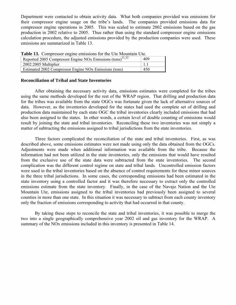
Department were contacted to obtain activity data. What both companies provided was emissions for their compressor engine usage on the tribe’s lands. The companies provided emissions data for compressor engine operations in 2005. This was scaled to estimate 2002 emissions based on the gas production in 2002 relative to 2005. Thus rather than using the standard compressor engine emissions calculation procedure, the adjusted emissions provided by the production companies were used. These emissions are summarized in Table 13. Table 13. Compressor engine emissions for the Ute Mountain Ute. Reported 2005 Compressor Engine NOx Emissions (tons)31,32 409 2002:2005 Multiplier 1.1 Estimated 2002 Compressor Engine NOx Emissions (tons) 450

Reconciliation of Tribal and State Inventories

After obtaining the necessary activity data, emissions estimates were completed for the tribes using the same methods developed for the rest of the WRAP region. That drilling and production data for the tribes was available from the state OGCs was fortunate given the lack of alternative sources of data. However, as the inventories developed for the states had used the complete set of drilling and production data maintained by each state OGC the tribal inventories clearly included emissions that had also been assigned to the states. In other words, a certain level of double counting of emissions would result by joining the state and tribal inventories. Reconciling these two inventories was not simply a matter of subtracting the emissions assigned to tribal jurisdictions from the state inventories.

Three factors complicated the reconciliation of the state and tribal inventories. First, as was described above, some emissions estimates were not made using only the data obtained from the OGCs. Adjustments were made when additional information was available from the tribe. Because the information had not been utilized in the state inventories, only the emissions that would have resulted from the exclusive use of the state data were subtracted from the state inventories. The second complication was the different control regime on state and tribal lands. Uncontrolled emission factors were used in the tribal inventories based on the absence of control requirements for these minor sources in the three tribal jurisdictions. In some cases, the corresponding emissions had been estimated in the state inventory using a controlled factor and it was therefore necessary to extract only the controlled emissions estimate from the state inventory. Finally, in the case of the Navajo Nation and the Ute Mountain Ute, emissions assigned to the tribal inventories had previously been assigned to several counties in more than one state. In this situation it was necessary to subtract from each county inventory only the fraction of emissions corresponding to activity that had occurred in that county.

By taking these steps to reconcile the state and tribal inventories, it was possible to merge the two into a single geographically comprehensive year 2002 oil and gas inventory for the WRAP. A summary of the NOx emissions included in this inventory is presented in Table 14.

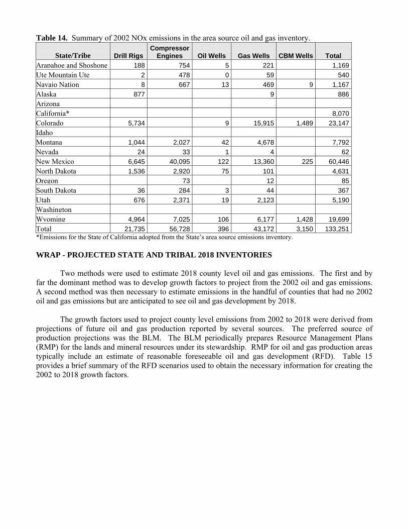
Table 14. Summary of 2002 NOx emissions in the area source oil and gas inventory.

State/Tribe Drill Rigs

Compressor Engines Oil Wells Gas Wells CBM Wells Total

Arapahoe and Shoshone 188 754 5 221 1,169Ute Mountain Ute 2 478 0 59 540Navajo Nation 8 667 13 469 9 1,167Alaska 877 9 886Arizona California* 8,070Colorado 5,734 9 15,915 1,489 23,147Idaho Montana 1,044 2,027 42 4,678 7,792Nevada 24 33 1 4 62New Mexico 6,645 40,095 122 13,360 225 60,446North Dakota 1,536 2,920 75 101 4,631Oregon 73 12 85South Dakota 36 284 3 44 367Utah 676 2,371 19 2,123 5,190Washington Wyoming 4,964 7,025 106 6,177 1,428 19,699Total 21,735 56,728 396 43,172 3,150 133,251*Emissions for the State of California adopted from the State’s area source emissions inventory. WRAP - PROJECTED STATE AND TRIBAL 2018 INVENTORIES

Two methods were used to estimate 2018 county level oil and gas emissions. The first and by far the dominant method was to develop growth factors to project from the 2002 oil and gas emissions. A second method was then necessary to estimate emissions in the handful of counties that had no 2002 oil and gas emissions but are anticipated to see oil and gas development by 2018.

The growth factors used to project county level emissions from 2002 to 2018 were derived from projections of future oil and gas production reported by several sources. The preferred source of production projections was the BLM. The BLM periodically prepares Resource Management Plans (RMP) for the lands and mineral resources under its stewardship. RMP for oil and gas production areas typically include an estimate of reasonable foreseeable oil and gas development (RFD). Table 15 provides a brief summary of the RFD scenarios used to obtain the necessary information for creating the 2002 to 2018 growth factors.

Table 15. BLM Resource Management Plans considered for use in projections.

RMP_NAME

Source Start Date End DateGas

Wells Oil

Wells CBM Wells

Wells Drilled

Northern San Juan Basin Coal Bed Methane Project

USDA FS, 2004 1/1/2004 1/1/2018 296 296

Pinedale RMP WY BLM, 2005 1/1/2006 1/1/2025 9800 9800Wyoming Powder River Basin Final EIS WY BLM, 2001 1/1/2002 1/1/2022 81000 81000White River Resource Area RMP EIS CO BLM, 1996 1/1/1996 1/1/2016 919 1100RMP EIS for Mineral Leasing and Development in Sierra and Otero Counties

NM BLM, 2003 1/1/2003 1/1/2023 36 48 105

Dakota Prairie Grasslands Oil and Gas Leasing

USDA FS, 2003 1/1/2003 1/1/2013 450 60 660

Farmington Proposed Resource Management Plan

NM BLM, 2003b 1/1/2002 1/1/2022 13271 380 2964 16615

Desolation Flats Natural Gas Field Development Project

WY BLM, 2004 1/1/2004 1/1/2024 308 474

Draft Vernal Resource Management Plan UT BLM, 2005 1/1/2006 1/1/2021 4345 2055 130 6530Jack Morrow Hills Coordinated Activity WY BLM, 2004b 7/1/2004 1/1/2021 107 50 255Wind River Natural Gas Project BIA, 2004 1/1/2005 1/1/2018 325 325Powder River and Billings Resource Management Plan

MT DEQ, 2003 1/1/2003 1/1/2023 800 18200 19000

Powder River and Billings Resource Management Plan

MT DEQ, 2003 1/1/2003 1/1/2023 250 6400 6650

Powder River and Billings Resource Management Plan

MT DEQ, 2003 1/1/2003 1/1/2023 150 150

As shown in Table 15, we obtained a number of RMPs covering a large portion of the WRAP

production areas. In addition to the BLM studies, the Alaska Department of Natural Resources prepares 20-year production forecasts that were used in this effort33. For the remaining areas, regional production forecasts published by the Energy Information Administration were used34. For those areas where EIA forecasts were the only source of data identified, separate oil and gas growth factors were calculated as the 2018 regional production forecast by the EIA divided by 2002 regional production reported by the EIA. There are three EIA growth regions in which some portion of emissions in that region were projected using EIA data. Growth factors developed for those regions based on the EIA’s production forecasts are shown in Table 16. Table 16. 2002 to 2018 oil and gas growth factors based on EIA forecasts.

Region Oil Production Gas ProductionRocky Mountain 1.334 1.458 Southwest 0.866 1.354 West Coast 0.601 0.568

Projections to 2018 based on the BLM RMP or Alaska DNR data were made using growth

factors derived from the proposed future development and the actual 2002 activity. In order to estimate the future number of wells, both the number of wells installed and the number of wells plugged and abandoned had to be estimated. As the RMPs do not include estimates of the number of wells that will be plugged and abandoned in future years, we used OGC data to estimate the number of wells plugged and abandoned annually at the county level. We then developed an estimate of the future number of wells in a production area based on the number of existing wells in 2002, the number of new wells anticipated by the RMP and the estimated number of wells that would be abandoned based on the assumed persistence of historical abandonment rates.

Because gas production at all well types drives compressor emissions, none of the three growth factors developed for oil wells, gas wells or CBM wells was alone representative of growth in

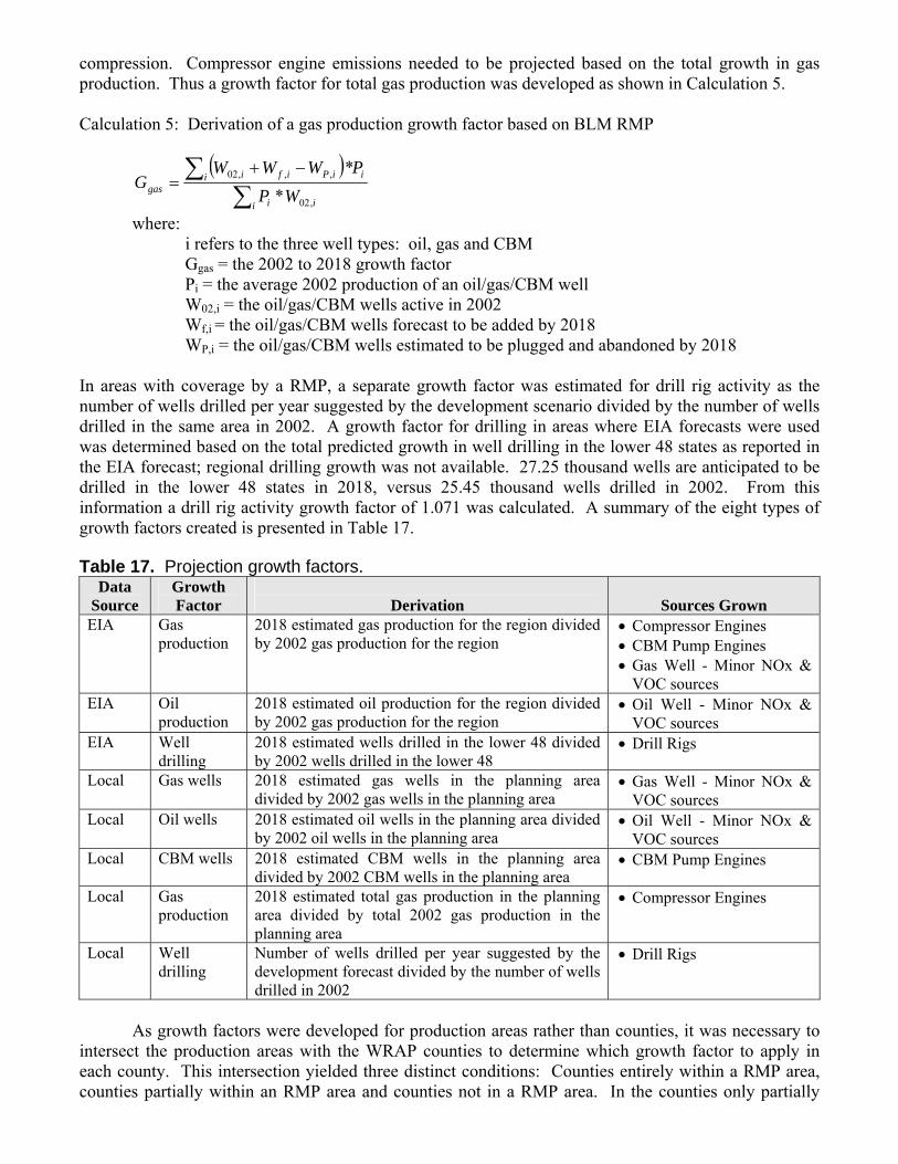
compression. Compressor engine emissions needed to be projected based on the total growth in gas production. Thus a growth factor for total gas production was developed as shown in Calculation 5. Calculation 5: Derivation of a gas production growth factor based on BLM RMP

( )∑

∑ −+=

i ii

ii iPifigas WP

PWWWG

,02

,,,02

**

where: i refers to the three well types: oil, gas and CBM

Ggas = the 2002 to 2018 growth factor Pi = the average 2002 production of an oil/gas/CBM well W02,i = the oil/gas/CBM wells active in 2002 Wf,i = the oil/gas/CBM wells forecast to be added by 2018 WP,i = the oil/gas/CBM wells estimated to be plugged and abandoned by 2018

In areas with coverage by a RMP, a separate growth factor was estimated for drill rig activity as the number of wells drilled per year suggested by the development scenario divided by the number of wells drilled in the same area in 2002. A growth factor for drilling in areas where EIA forecasts were used was determined based on the total predicted growth in well drilling in the lower 48 states as reported in the EIA forecast; regional drilling growth was not available. 27.25 thousand wells are anticipated to be drilled in the lower 48 states in 2018, versus 25.45 thousand wells drilled in 2002. From this information a drill rig activity growth factor of 1.071 was calculated. A summary of the eight types of growth factors created is presented in Table 17. Table 17. Projection growth factors.

Data Source

Growth Factor

Derivation Sources Grown

EIA Gas production

2018 estimated gas production for the region divided by 2002 gas production for the region

• Compressor Engines • CBM Pump Engines • Gas Well - Minor NOx &

VOC sources EIA Oil

production 2018 estimated oil production for the region divided by 2002 gas production for the region

• Oil Well - Minor NOx & VOC sources

EIA Well drilling

2018 estimated wells drilled in the lower 48 divided by 2002 wells drilled in the lower 48

• Drill Rigs

Local Gas wells 2018 estimated gas wells in the planning area divided by 2002 gas wells in the planning area

• Gas Well - Minor NOx & VOC sources

Local Oil wells 2018 estimated oil wells in the planning area divided by 2002 oil wells in the planning area

• Oil Well - Minor NOx & VOC sources

Local CBM wells 2018 estimated CBM wells in the planning area divided by 2002 CBM wells in the planning area

• CBM Pump Engines

Local Gas production

2018 estimated total gas production in the planning area divided by total 2002 gas production in the planning area

• Compressor Engines

Local Well drilling

Number of wells drilled per year suggested by the development forecast divided by the number of wells drilled in 2002

• Drill Rigs

As growth factors were developed for production areas rather than counties, it was necessary to

intersect the production areas with the WRAP counties to determine which growth factor to apply in each county. This intersection yielded three distinct conditions: Counties entirely within a RMP area, counties partially within an RMP area and counties not in a RMP area. In the counties only partially

intersected by a RMP area, it was necessary to apply BLM-based growth factors to the fraction of the wells in the RMP area and EIA-based growth factors to the remaining wells. Independent 2018 emissions estimates

There were some areas where an RMP predicted oil and gas development, but no oil or gas wells existed in 2002. In those cases, the growth factor approach could not be applied. Instead, a method was developed whereby emissions were estimated based on the development forecast by the RMP and the average emissions associated with similar oil and gas sources in the same state. The general form of the calculation used to estimate 2018 emissions in these counties is presented as Calculation 6. Calculation 6. General formula for independent estimates of 2018 emissions

PPP EDE ,02,18 *= where: E18,P = the emissions from a process in 2018 D = the forecast development of process p in the area E02,P = the state average emissions from process p in 2002

This number of 2018 oil, gas, CBM and/or drilled wells predicted by the RMP served as the activity measure for the 2018 emissions estimates. State specific emission factors were derived by dividing 2002 state total process specific emissions by the number of 2002 oil, gas, CBM or drilled wells. In the case of CBM wells, the lack of 2002 emissions in some states required that an emission factor be adopted from another area. In these cases, data from the State of Wyoming was adopted. The emission factors that resulted for NOx are shown in Table 18. Emission factors for other pollutants were developed by the same approach. Table 18. State NOx emission factors used to estimate 2018 emissions.

Process Drill Rigs Compressor Engines

Oil Well Heaters

Gas Well Heaters

Gas Well Completion Flaring & Venting

CBM Pump Engines

Units tons/well drilled

tons/MCF tons/well tons/well tons/well tons/well

Montana 2.26 2.34x10-5 0.011 0.859 0.147 0.12 New Mexico 7.12 2.34x10-5 0.008 0.868 0.046 0.12 North Dakota 9.78 2.34x10-5 0.867 0.031 0.12 Utah 5.37 4.11x10-6 0.015 0.12

The emission factors in Table 18 were combined with development forecasts as shown in

Calculation 6 to produce the county level emissions. These emissions estimates were then combined with the projected 2018 emissions to produce a comprehensive 2018 area source oil and gas emission inventory. Future Year Emission Controls

Implementation of new federal and state control programs will have a substantial impact on future emissions. Known state and federal emissions control estimates were incorporated into the base case projections for 2018. A summary of the controls identified and the actions taken to incorporate them into the 2018 projections is provided in Table 19. These controls add to those previously identified in the 2002 inventory. Thus, although not presented here, the state-specific controls included in the 2002 inventory were adopted by the 2018 inventory.

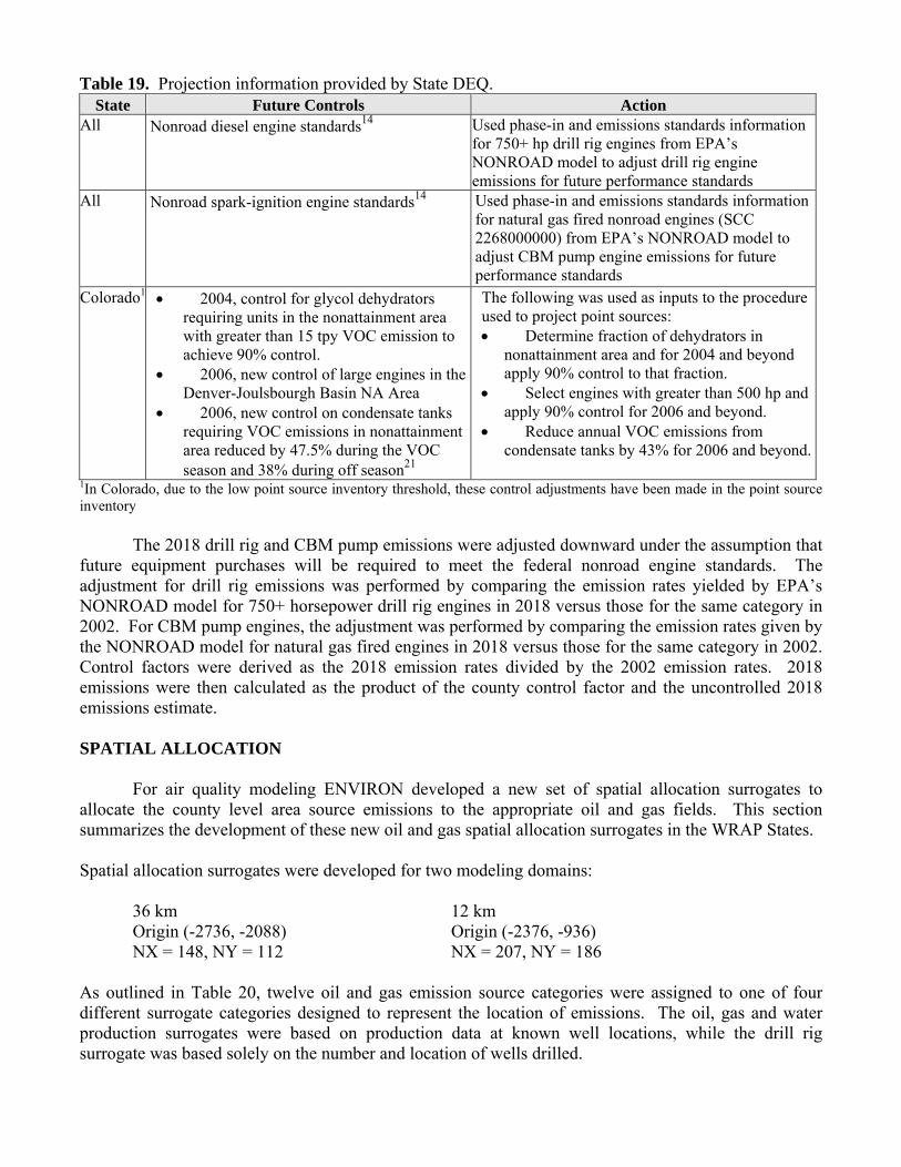
Table 19. Projection information provided by State DEQ.

State Future Controls Action All Nonroad diesel engine standards14 Used phase-in and emissions standards information

for 750+ hp drill rig engines from EPA’s NONROAD model to adjust drill rig engine emissions for future performance standards

All Nonroad spark-ignition engine standards14 Used phase-in and emissions standards information for natural gas fired nonroad engines (SCC 2268000000) from EPA’s NONROAD model to adjust CBM pump engine emissions for future performance standards

Colorado1 • 2004, control for glycol dehydrators requiring units in the nonattainment area with greater than 15 tpy VOC emission to achieve 90% control.

• 2006, new control of large engines in the Denver-Joulsbourgh Basin NA Area

• 2006, new control on condensate tanks requiring VOC emissions in nonattainment area reduced by 47.5% during the VOC season and 38% during off season21

The following was used as inputs to the procedure used to project point sources: • Determine fraction of dehydrators in

nonattainment area and for 2004 and beyond apply 90% control to that fraction.

• Select engines with greater than 500 hp and apply 90% control for 2006 and beyond.

• Reduce annual VOC emissions from condensate tanks by 43% for 2006 and beyond.

1In Colorado, due to the low point source inventory threshold, these control adjustments have been made in the point source inventory

The 2018 drill rig and CBM pump emissions were adjusted downward under the assumption that future equipment purchases will be required to meet the federal nonroad engine standards. The adjustment for drill rig emissions was performed by comparing the emission rates yielded by EPA’s NONROAD model for 750+ horsepower drill rig engines in 2018 versus those for the same category in 2002. For CBM pump engines, the adjustment was performed by comparing the emission rates given by the NONROAD model for natural gas fired engines in 2018 versus those for the same category in 2002. Control factors were derived as the 2018 emission rates divided by the 2002 emission rates. 2018 emissions were then calculated as the product of the county control factor and the uncontrolled 2018 emissions estimate. SPATIAL ALLOCATION

For air quality modeling ENVIRON developed a new set of spatial allocation surrogates to allocate the county level area source emissions to the appropriate oil and gas fields. This section summarizes the development of these new oil and gas spatial allocation surrogates in the WRAP States. Spatial allocation surrogates were developed for two modeling domains:

36 km 12 km Origin (-2736, -2088) Origin (-2376, -936) NX = 148, NY = 112 NX = 207, NY = 186

As outlined in Table 20, twelve oil and gas emission source categories were assigned to one of four different surrogate categories designed to represent the location of emissions. The oil, gas and water production surrogates were based on production data at known well locations, while the drill rig surrogate was based solely on the number and location of wells drilled.

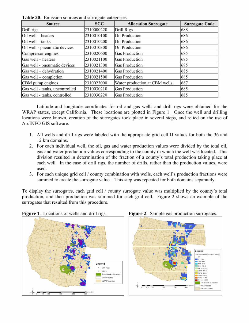
Table 20. Emission sources and surrogate categories. Source SCC Allocation Surrogate Surrogate Code

Drill rigs 2310000220 Drill Rigs 688 Oil well – heaters 2310010100 Oil Production 686 Oil well – tanks 2310010200 Oil Production 686 Oil well - pneumatic devices 2310010300 Oil Production 686 Compressor engines 2310020600 Gas Production 685 Gas well – heaters 2310021100 Gas Production 685 Gas well - pneumatic devices 2310021300 Gas Production 685 Gas well – dehydration 2310021400 Gas Production 685 Gas well – completion 2310021500 Gas Production 685 CBM pump engines 2310023000 Water production at CBM wells 687 Gas well - tanks, uncontrolled 2310030210 Gas Production 685 Gas well - tanks, controlled 2310030220 Gas Production 685

Latitude and longitude coordinates for oil and gas wells and drill rigs were obtained for the WRAP states, except California. These locations are plotted in Figure 1. Once the well and drilling locations were known, creation of the surrogates took place in several steps, and relied on the use of ArcINFO GIS software.

1. All wells and drill rigs were labeled with the appropriate grid cell IJ values for both the 36 and 12 km domains.

2. For each individual well, the oil, gas and water production values were divided by the total oil, gas and water production values corresponding to the county in which the well was located. This division resulted in determination of the fraction of a county’s total production taking place at each well. In the case of drill rigs, the number of drills, rather than the production values, were used.

3. For each unique grid cell / county combination with wells, each well’s production fractions were summed to create the surrogate value. This step was repeated for both domains separately.

To display the surrogates, each grid cell / county surrogate value was multiplied by the county’s total production, and then production was summed for each grid cell. Figure 2 shows an example of the surrogates that resulted from this procedure. Figure 1. Locations of wells and drill rigs. Figure 2. Sample gas production surrogates.

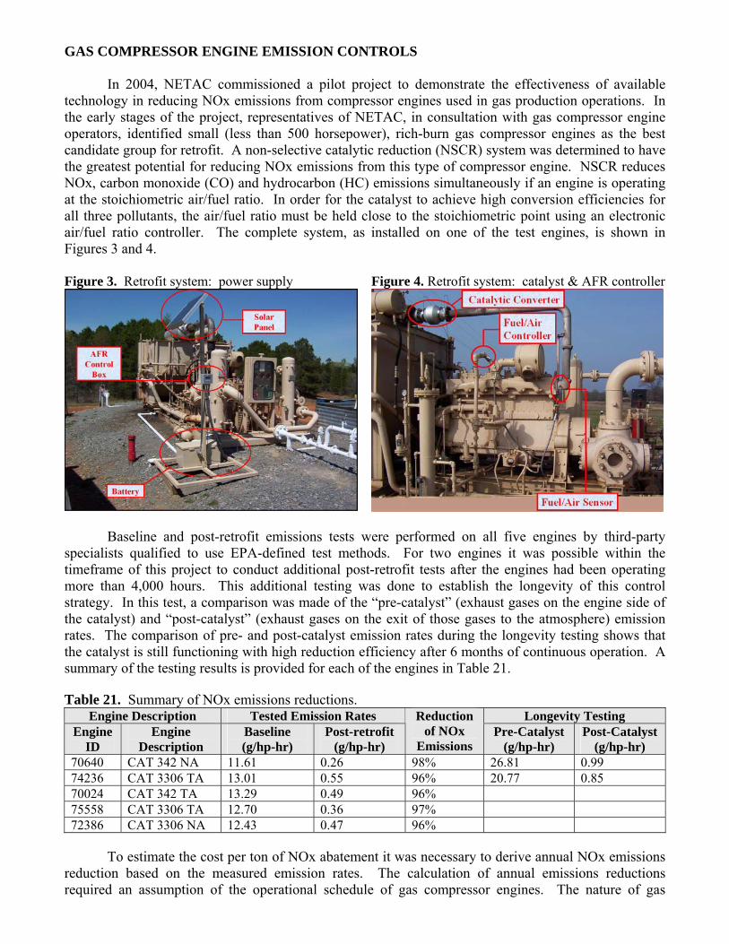
GAS COMPRESSOR ENGINE EMISSION CONTROLS

In 2004, NETAC commissioned a pilot project to demonstrate the effectiveness of available technology in reducing NOx emissions from compressor engines used in gas production operations. In the early stages of the project, representatives of NETAC, in consultation with gas compressor engine operators, identified small (less than 500 horsepower), rich-burn gas compressor engines as the best candidate group for retrofit. A non-selective catalytic reduction (NSCR) system was determined to have the greatest potential for reducing NOx emissions from this type of compressor engine. NSCR reduces NOx, carbon monoxide (CO) and hydrocarbon (HC) emissions simultaneously if an engine is operating at the stoichiometric air/fuel ratio. In order for the catalyst to achieve high conversion efficiencies for all three pollutants, the air/fuel ratio must be held close to the stoichiometric point using an electronic air/fuel ratio controller. The complete system, as installed on one of the test engines, is shown in Figures 3 and 4. Figure 3. Retrofit system: power supply Figure 4. Retrofit system: catalyst & AFR controller

Baseline and post-retrofit emissions tests were performed on all five engines by third-party specialists qualified to use EPA-defined test methods. For two engines it was possible within the timeframe of this project to conduct additional post-retrofit tests after the engines had been operating more than 4,000 hours. This additional testing was done to establish the longevity of this control strategy. In this test, a comparison was made of the “pre-catalyst” (exhaust gases on the engine side of the catalyst) and “post-catalyst” (exhaust gases on the exit of those gases to the atmosphere) emission rates. The comparison of pre- and post-catalyst emission rates during the longevity testing shows that the catalyst is still functioning with high reduction efficiency after 6 months of continuous operation. A summary of the testing results is provided for each of the engines in Table 21. Table 21. Summary of NOx emissions reductions.

Engine Description Tested Emission Rates Longevity Testing Engine

ID Engine

Description Baseline (g/hp-hr)

Post-retrofit (g/hp-hr)

Reduction of NOx

Emissions Pre-Catalyst

(g/hp-hr) Post-Catalyst

(g/hp-hr) 70640 CAT 342 NA 11.61 0.26 98% 26.81 0.99 74236 CAT 3306 TA 13.01 0.55 96% 20.77 0.85 70024 CAT 342 TA 13.29 0.49 96% 75558 CAT 3306 TA 12.70 0.36 97% 72386 CAT 3306 NA 12.43 0.47 96%

To estimate the cost per ton of NOx abatement it was necessary to derive annual NOx emissions

reduction based on the measured emission rates. The calculation of annual emissions reductions required an assumption of the operational schedule of gas compressor engines. The nature of gas

production and information provided by gas compressor operators suggests that gas compressor engines operate nearly year-round. The exception to this is periods when the engines are shut down for repairs or maintenance. For the purposes of this cost effectiveness calculation it was assumed that the engines will operate 8,000 of 8,760 hours per year. The loading of the compressor engines was estimated based on the average loading at the time of emissions testing. The average load before and after installation of the catalyst ranged from 41 to 66 percent for the five engines. Using these assumptions and the emission factors determined from emissions testing, annual emissions reductions were estimated for each of the engines. The average annual emissions reduction determined for the five engines was 12.3 tons NOx per year.

For the five engines, the average cost of the control equipment and engine modifications, including air/fuel ratio controllers and the solar power units to power those controllers, was $7,672. The estimated cost of the labor required to install the equipment was $1,280 per engine. The average upfront cost of the retrofit was thus $8,952 per engine. The maintenance costs of this control system are limited to those of several regularly occurring tasks. These tasks include biannual cleaning of the catalyst, quarterly replacement of the oxygen sensor and replacement of the solar power unit’s battery every four years. When the upfront and maintenance costs were annualized over an assumed five-year project life at a discount rate of 3 percent, the total annual cost estimated for the retrofit was $2,250 per engine.

The average emissions reduction of the compressor engine retrofit was derived from the results of carefully planned emissions testing. The annual cost of the retrofit was estimated based on actual installation costs and anticipated maintenance costs. From these figures it was a simple matter to estimate the cost effectiveness. The average annualized cost of installation and maintenance of $2,250, divided by the average annual emission reduction, 12.3 tons NOx, yielded a cost of $183 per one-ton reduction of NOx emissions. Thus this pilot project demonstrated that the installation of catalysts on gas compressor engines is an exceptionally cost effective strategy for achieving NOx emission reductions. CONCLUSIONS

Table 22 compares the results of the WRAP oil and gas inventory effort with the oil and gas emissions in the inventories that were previously available. Total NOx emissions estimated by this

Table 22. Change in oil and gas NOx emissions in the 2002 inventory as a result of this study.

State/Tribe Area Point Total Area Point Total Total PercentArapahoe and Shoshone* 1,169 54 1,223 NA NA NA 1,223 NA

Navajo Nation* 540 6,382 6,922 NA NA NA 6,922 NA

Ute Mountain Ute* 1,167 - 1,167 NA NA NA 1,167 NA

Alaska 886 45,822 46,708 45,822 45,822 886 2%Arizona 2,735 2,735 2,735 2,735 - 0%California** 8,070 16,707 24,777 8,070 16,707 24,777 - 0%Colorado 23,147 25,955 49,102 25,955 25,955 23,147 89%Idaho 2,590 2,590 2,590 2,590 - 0%Montana 7,792 4,275 12,067 4,275 4,275 7,792 182%Nevada 62 83 145 83 83 62 75%New Mexico 60,446 57,173 117,619 57,173 57,173 60,446 106%North Dakota 4,631 4,739 9,369 4,739 4,739 4,631 98%Oregon 85 1,182 1,267 1,182 1,182 85 7%South Dakota 367 323 690 323 323 367 114%Utah 5,190 3,311 8,500 3,311 3,311 5,190 157%Washington 1,281 1,281 1,281 1,281 - 0%Wyoming 19,699 15,015 34,715 6,409 15,015 21,424 13,290 62%Total 133,251 187,627 320,878 14,479 181,191 195,670 125,209 64%

WRAP Oil and Gas Inventory Oil and Gas in Previous InventoryChange in Oil and

Gas Emissions

*Point source inventories for the tribes were compiled by the Institute for Tribal Environmental Professionals. **Area source emissions in WRAP Oil and Gas Inventory adopted from data submitted by the California ARB.

inventory of oil and gas emissions represent a 64 percent increase in inventoried oil and gas emissions. The increases in some of the main oil and gas producing states are even more dramatic. Emissions in Montana, North Dakota and Utah increased by 182, 98 and 157 percent as a result of this effort. Oil and gas NOx emissions estimated for the State of New Mexico increased by over 60,000 tons.

Table 23 shows the percent change in NOx emissions projected to occur from 2002 to 2018. Oil and gas area source NOx emissions estimated for 2018 show a 115 percent increase over 2002 levels. In the total oil and gas emissions, the projected increase in area source emissions is partially offset by a greater than 50 thousand ton decrease in NOx emissions predicted for point sources. The forecast area source and overall increases are most substantial in places where recent development plans predict large-scale oil and gas projects in future years. Such is the case in Montana and Wyoming where major development is anticipated for the Powder River Basin and the Jonah-Pinedale area. Table 23. Change in oil and gas NOx emissions from 2002 to 2018.

Tribes 127% 33% 157% -86% 128% -26% 19%Alaska -35% -79% -36% -20% -21%Arizona 27% 27%

California -20% -46%Colorado -29% 47% -88% 20% -39% -11%

Idaho -33% -33%Montana 839% 248% 62% 292% -40% 174%Nevada 46% -31% 42% 16% 68% 46%

New Mexico 155% 18% 111% -91% 129% -36% 49%North Dakota 131% -16% 261% 87% -38% 24%

Oregon -43% -43% -43% -49% -48%South Dakota 46% -31% 45% 38% -4% 19%

Utah 100% 227% 191% 154% -30% 82%Washington -45% -45%Wyoming 366% 50% 194% -37% 202% -35% 99%

Total 200% 26% 99% -57% 115% -30% 30%

CBM Pump Engines

Area Source

Point Source TOTALState/Tribe

Compressor Engines Drill Rigs Wellhead

The inventories produced by these projects indicate the importance of oil and gas production as a source of emission in the western region. As this was the first effort to develop a regionally consistent emission inventory for oil and gas area sources and resources were limited, this inventory is neither as comprehensive nor as accurate as it might be with more resources. The inventories and the methodology used represent a first step toward a better understanding of oil and gas emissions. At a minimum, these results indicate that many states and tribes will need to carefully evaluate the impact of existing and future oil and gas production as they work to meet their air quality goals. The methods described here for compiling oil and gas emissions inventories, projecting future emissions, spatially allocating emissions, and controlling emissions from gas compressor engines should provide useful tools for those future studies. REFERENCES 1. EIA, 2006. Natural Gas Gross Withdrawals and Production, Energy Information

Administration. April. Internet address: http://tonto.eia.doe.gov/dnav/ng/ng_prod_sum_a_EPG0_FGW_mmcf_a.htm.

2. EIA, 2006b. “Crude Oil Production”, Energy Information Administration. March. Internet

address: http://tonto.eia.doe.gov/dnav/pet/pet_crd_crpdn_adc_mbbl_a.htm. 3. Schlichtemeier, C. 2005. Wyoming Department of Environmental Quality, WY.

CSCHLI@state.wy.us April 8, personal communication.

4. Meyer, R. 2005. Wyoming Oil and Gas Conservation Commission, WY. rmeyer2@state.wy.us

March 18, personal communication. 5. NMOGA, 2003. “Inventory of Unpermitted Sources in the San Juan Basin”; Prepared for the

New Mexico Environmental Department by the New Mexico Oil and Gas Association, NM. 6. NMT, 2005. GO-TECH, Online oil and gas production database for the State of New Mexico,

New Mexico Institute of Mining and Technology, NM. Internet address: http://octane.nmt.edu/data/ongard/general.asp.

7. Schlichtemeier, C. 2005b. Wyoming Department of Environmental Quality, WY.

CSCHLI@state.wy.us March 14, personal communication. 8. Anderson, T. 2005. Utah Department of Environmental Quality, UT. TDAnderson@utah.gov

May 9, personal communication. 9. Doyle, R. 2005. Colorado Department of Health and Environment, CO. roy.Doyle@state.co.us

March 25, personal communication. 10. Maunder, T. 2005. Alaska Oil and Gas Conservation Commission, AK.

tom_maunder@admin.state.ak.us March 18, personal communication. 11. Walker, B. 2005. Alaska Department of Environmental Conservation, AK. (B. Walker - 907-

465-5124), March 18, personal communication. 12. Richmond, 2005. Montana Board of Oil and Gas Conservation, MT. February, personal

communication. 13. Daniels, 2005. Utah Department of Natural Resources, UT. March personal communication. 14. EPA NONROAD, 2004. “EPA’s NONROAD 2004 Emissions Model”, U.S. Environmental

Protection Agency, Research Triangle Park, NC. Internet address: http://www.epa.gov/otaq/nonrdmdl.htm.

15. Schlichtemeier, C. 2005c. Wyoming Department of Environmental Quality, WY.

(CSCHLI@state.wy.us) November 10, 2004, personal communication. 16. Gantner, 2005. New Mexico Oil and Gas Association, NM. June, personal communication. 17. Olson, 2005. Williams Exploration and Production, Gillette, WY. June, personal

communication. 18. Strong, 2005. Wyoming Oil and Gas Conservation Commission, WY. June, personal

communication. 19. Weatherford, 2005. Weatherford U.S., Gillette, Wyoming, June, personal communication. 20. WY DEQ, 2004. Wyoming Department of Environmental Quality, Air Quality Division,

Cheyenne, Wyoming, personal communication.

21. Thayer, D. 2005b. Colorado Department of Health and Environment, CO (david.thayer@state.co.us) personal communication.

22. Aguirre, D. 2005. Montana Department of Environmental Quality, MT. (daguirre@mt.gov),

March 9, personal communication. 23. Pingree, C. 2005. Shoshone Oil and Gas Commission (C. Pingree - 307-332-3917) June,

personal communication.

24. Roman, F. 2005. Wind River Environmental Quality Commission (Fernando Air Quality Coordinator, 307-332-3164), May, personal communication.

25. Bob, G.L 2005. Navajo Nation Minerals Department (Navajo Nation, Minerals Department,

928-871-7305), April, personal communication. 26. NM OCD, 2004. “AllWells050424.zip”. New Mexico Energy, Minerals and Natural Resources

Department, Oil Conservation Division. Internet address: ftp://164.64.103.5/public/ocd/Data/. 27. Dennison. J. 2005b. Navajo Nation Minerals Department. (Navajo Nation, Minerals

Department, 928-871-7096) July, personal communication. 28. Simon; G. 2005. Ute Mt Ute Energy Department. (Petroleum Geologist; 505-821-2555). May

4, personal communication. 29. Kerr, T. 2005. Colorado Oil and Gas Conservation Commission, CO. (thom.kerr@state.co.us),

March 21, personal communication. 30. Rice; T. 2005. Ute Mt. Ute Environmental Department, (Ute Mt. Ute Environmental

Department; umutenv@fone.net) April 11, personal communication.

31. Hasely, E. 2005. Burlington Resources Inc., NM. (Environmental Advisor; Burlington Resources; Lhasely@br-inc.com) June 6, personal communication.

32. Agee, D. 2005. XTO Energy Inc., NM. (D. Agee; XTO; 817-885-2285) June 20, personal

communication.

33. AK DNR, 2004. Alaska: “Oil and Gas Report”, Alaska Department of Natural Resources, Division of Oil & Gas. December. Internet address: http://www.dog.dnr.state.ak.us/oil/products/publications/annual/report.htm.

34. EIA, 2005. “Annual Energy Outlook 2005 with Projections to 2025.” Energy Information

Administration. January. Internet address: http://www.eia.doe.gov/oiaf/aeo/index.html.

KEY WORDS Oil Production Natural Gas Production Coalbed Methane Emission Inventory Regional Haze Projections Spatial Surrogates Compressor Engines Non Selective Catalytic Reduction