EMIS - Excel

Reference Guide

Create Source Data Files

Create a Source Data File from your Student Software program.

Current Year (valid as of the day pulled)

Previous Year (used when reviewing data that crosses over)

Pull complete set of data with NO filters

Frequently needed source data fields...

Legal First Name Student Status District Admission Date EMIS Situation

Legal Last Name EMIS State Grade Level Admission Reason District Relationship

Student Number EMIS Grade Next Year Admitted From IRN How Received

EMIS ID Building District Withdraw Date (FS) Percent of Time

Birthdate State Student ID Withdraw Reason Attending Building IRN

Gender Effective Start Date (FS) Withdrawn to IRN District of Residence

How Received IRN Sent to Reason Sent to IRN Sent to Percent of Time

Disability Condition Disadvantagement Limited English Proficiency Reporting Calendar

Attendance Pattern Retained Status Fiscal Year Began 9th Majority of Attendance IRN

Report to EMIS EMIS Ethnicity Graduation Date Math Diagnostic Result

Diploma Type Graduation Year County of Residence Reading Diagnostic Result

Exempted from Phys Ed Core Grad Requirement Exempt Writing Diagnostic Result

Are there other fields that you would like to include in your Source Data File, but your Student Software doesn’t pull it with your

main search?

Add additional data from other data sources...

Assessment files from vendors

Class List / Course Rosters

Data Collector Collection Reviews

ODDEX-SOES

By combining multiple data sources into one Source Data File, EMIS crosschecks can be done in BEFORE collecting and sub-

mitting. Below are a few examples:

Calendars—Grade level specific, EMIS Situation

Special Ed— Disability Condition, Dates, Assessment

TGRG—Diagnostics, RIMPS, Assessments, Retentions

What do I do with this report??? Your source data is always the place to go to compare what is being reported to the various re-

ports and files that come back from the Data Collector and Secure Data Center.

Reports may come back with NO student names…V-Lookup is an easy way to import names quickly.

VLOOKUP can be used for other reports as well to add additional information to create an even more data driven report.

1. Open Source Data File (File A) - Sort Ascending by SSID and save (Do NOT close file).

2. Open Report missing Student Names (File B) - Sort Ascending by SSID and save (Do NOT close file).

3. Create new workbook in File B and rename it SOURCE DATA.

4. Copy and paste the data from File A into the Source Data worksheet tab in File B.

5. Move State Student ID to column A (Both files). Always move the SSID field to column A first in the files you will be using.

6. Insert and label two columns for names. (File B)

7. In Cell B2 of File B (LAST NAME) click on the function icon.

A. The Insert Function pop-up should appear. Select VLOOKUP and OK.

B. The Function Arguments popup should now appear. DO NOT HIT ENTER/OK UNTIL ALL FOUR VALUES ARE INSERTED.

C. Lookup_value - File B, click in Cell A2 (SSID)

D. Table_array - File A, Highlight area that you want the LOOKUP to look at

E. Col_index_num - File A, 2 (column number the LAST NAME is in)

F. Range_lookup - FALSE

8. Drag or copy down the VLOOKUP result to the end of column B in File B.

9. Follow the same steps to come up with the First Name column for File B.

V-Lookup

7A &B

7C

7E

7D

7F

8

Conditional Formatting

Missing something that you don’t know you’re missing?

Use Conditional formatting to highlight who is on both reports...and

find out who isn’t.

K-3 Literacy SDC List VS Source Data List

Source Data—Main Report

Known SSID’s—SDC List

1. Copy and paste the list of known SSID’s at the bottom of your

main report.

2. Select Column A (SSID’s to compare)

3. Go to Home > Conditional Formatting > Highlight Cell Rules >

Duplicate Values

4. At the Duplicate Values prompt, it should default to “Duplicate”

values with “Light Red Fill with Dark Red Text”. Select “OK”

5. All SSID’s that are in the SDC List will

be highlighted in light red and have

dark red text.

6. Are students counting that should

count? Who is missing? Who is on

the list but shouldn’t be?

1 & 2

3, 4 & 5

6

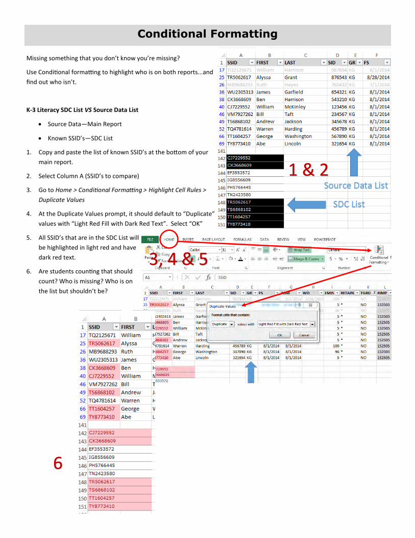
Pivot Table

Need a quick summary analysis of data? Start small and work your way up to complex Pivot Tables.

Sample source data for this example is from a Career Center and includes the following fields:

First Name—Last Name—Student ID—Ethnicity—Gender—Grade—SSID—EMIS Situation—District of Residence

Summary we want to see: Ethnicity By Grade Level

Two options of creating a Pivot Table are “Recommended Pivot Table” and “Manually create Pivot Table”. Both can be found under

Insert > Tables > Recommended Pivot Table or Pivot Table

By selecting “Recommended Pivot Table”, you

are able to hover over different pre-selected

views of potential Pivot Tables. A new work-

sheet tab will open at the bottom of your docu-

ment and the recommended Pivot Table will

drop in.

This particular Pivot Table recommendation will show

the Ethnicity by Grade Levels.

Row = Grade Level

Column = Ethnicity

Values = Total by Last (Name)

Fields can be moved between

Filters, Columns, Rows and

Values to give a different look

to the table.

Additional EMIS Tips, Tricks & Shortcuts

1. Need to change student names from all upper case to “Proper” case?

Insert additional column(s) next to the names.

In cell C2, type =PROPER(A2)

In cell D2, type =PROPER(B2)

HARRY POTTER should now be Harry Potter

2. How to calculate how many days are between two dates?

D2 = Beginning of the school year (8/17/16)

E2 = End Date (2/1/17)

In cell F2, type =DAYS(E2,D2)

The total number of calendar days will populate. Drag the result

down the column to fill in the rest of the fields.

Pivot Table (continued)

Creating your own Pivot Table can be intimidating, but the

more you work with it and know what you want to see as

an end result the more comfortable you will be.

This Pivot Table created manually allows the user to filter

by EMIS Situation, Grade Level, or District of Residence.

By creating Pivot Tables, your Source Data always remains un-

touched unless you are in that worksheet making changes.

TGRG Diagnostics 30-day Rule

3. Need to know a date in a future year?

If you need the end date for an IEP, it is 1 year minus 1 day from the Event date.

In cell I3, type =DATE(YEAR(F3)+1,MONTH(F3),DAY(F3-1)

For an ETR, it is 3 years minus 1 day from

the Event date

In cell N3, type =DATE(YEAR(F3)

+3,MONTH(F3),DAY(F3-1)

TIEP and TETR have to be entered manu-

ally since the Event Date is the Adoption

Date.

4. Want to get a headstart on your 5 & 6 year

olds for Federal Child Count? To help you de-

termine a students age as of a certain date

you will find the formula listed below as a helpful addition to your

Source Data.

Known Data: Date of Birth, Due date of 10/31/16,

Disability = Yes, Grade = Kindergarten

In cell I3, type =DATEDIF(H3,I2,”Y”)

Additional EMIS Tips, Tricks & Shortcuts

End Date for an IEP or ETR

Age for Federal Child Count

Additional EMIS Tips, Tricks & Shortcuts

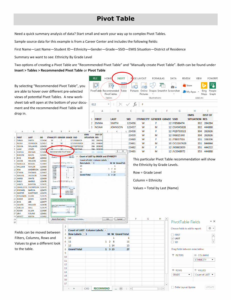
5. Have a large amount of data that you would like to see as a table?

Open your worksheet and select INSERT > TABLE

The range of data to be included in the table will auto-populate. Click OK.

Your worksheet will now be in a Table format. You can select various types

by going to TABLE TOOLS > DESIGN > TABLE STYLES.

To change the table back to a worksheet with no filters but keeping the style

of the table, you would select TABLE TOOLS > DESIGN > Tools > Convert to

Range.

When converting back to a worksheet a pop-up will appear asking if you

want to convert the table to a normal range. Select YES.

You’ll notice the filters are gone, but the table style remains.

6. Want a quick AVERAGE, COUNT, or SUM of a column?

Highlight the column that you would like this data on.

Look in the bottom right corner of the worksheet and the

AVERAGE, COUNT and/or SUM will appear.

AVERAGE is the average of the selected cells.

COUNT is the number of selected cells that contain data.

SUM is the sum of the selected cells

To add additional settings to the Status Bar, right click any-

where in the bar and check or un-check what you would

like to see.

New Table Style converted back to worksheet.

Which Tab is it under???

FILE

Info

New

Open

Save

Save As

Print

HOME

Clipboard

Font

Alignment

Number

Styles

Cells

Editing

Frequently Used Tools for EMIS

HOME DATA VIEW

Fill color Sort Page Break Preview

Text Color Filter Zoom

Wrap Text Text to Columns Arrange all

Conditional Formatting Freeze Panes

Sort & Filter

INSERT FORMULAS PAGE LAYOUT

Pivot Table Insert Function Themes

Text Box AutoSum Orientation

INSERT

Tables

Add-Ins

Charts

Sparklines

Filters

Links

Text

Symbols

PAGE LAYOUT

Themes

Page Setup

Scale to Fit

Sheet Options

Arrange

FORMULAS

Function Library

Defined Names

Formula Auditing

Calculation

DATA

Get External Data

Connections

Sort & Filter

Data Tools

Outline

REVIEW

Proofing

Language

Comments

Changes

VIEW

Workbook Views

Show

Zoom

Window

Macros

POWERPIVOT

Data Model

Calculations

Slicer Aligment

Tables

Relationships

Settings

When in doubt...“HELP” yourself out with Excel Help.

Excel Reference Guide

File tab

Zoom Slider

Rows

Columns

Quick Access Toolbar

Formula Bar

Ribbon

Worksheet Tabs

Open Workbook <Ctrl> + < O > To Cell A1 <Ctrl> + <Home>

Create New Workbook <Ctrl> + < N > To Last Cell <Ctrl> + <End>

Save <Ctrl> + < S > Cut <Ctrl> + < X >

Preview and Print <Ctrl> + < P > Copy <Ctrl> + < C >

Close Workbook <Ctrl> + < W > Paste <Ctrl> + < V >

Right One Cell <Tab> Undo <Ctrl> + < Z >

Left One Cell <Shift> + <Tab> Redo <Ctrl> + < Y >

Up One Cell <Shift> + Enter Find <Ctrl> + < F >

Select All <Ctrl> + < A > Replace <Ctrl> + < H >

Select Entire Row <Shift> + <Space> Bold <Ctrl> + < B >

Select entire column <Ctrl> + <Space> Italics <Ctrl> + < I >

Fill Right <Ctrl> + < R > Underline <Ctrl> + < U >

Keyboard Shortcuts

Status Bar

**Short cut to frequently used items, “Right Click”**

Copy, Cut, Paste, Font Size, Font Color, Fill Color are just a few options available when you right click in your workbook or

cell.