Embed Size (px)
Citation preview
Effect of Implementation of Common Core
Case Study: California Emily Kaar* 3/12/2017
*Many thanks to Giovanni Peri for his continual help on this paper and to Vasco Yasenov for this help with my data.
1
Abstract:
Key words: Education, Inequality, Common Core, SBA
This paper examines the effect of Common Core State Standards on end-‐of-‐year test scores for high school students in California. I find that for the whole population there was not a significant effect on scores, but for minority students, scores increased.
2
In 2015, the United Sates Federal Government spent $122 billion on education, which
corresponds to 3.8% of total government spending. Education was the third largest spending
category after health care and pensions for the Federal Government. In addition to federal
education spending, state and local governments spend approximately $985 billion every year.
In aggregate, education is the largest spending category for state and local governments across
the US. For this amount of expenditure, it is important that the money is spent efficiently. As
taxes create inefficiency in the economy, it is imperative for a well-functioning economy that tax
money is spent well in order to create growth for the economy.
Education is an engine of growth because it is an investment. Education builds human
capital which increases the productivity of workers. Studies have found that increased levels of
education mean higher labor force participation, lower unemployment rates, and higher wages
(Borjas 1996). The secondary effects of this human capital accumulation are increased economic
growth from more educated workers, which raises the standard of living. Additionally, higher
wages are correlated with positive social outcomes such as lower crime rates (Deming 2011) and
increased voter turnout (Sondheimer and Green 2010). Education also is supposed to provide
opportunities to everyone, in order to foster upward mobility. And indeed, research has shown
that “education plays a crucial role in improving labor market outcomes for both men and
women and for workers across racial groups” (Borjas 1996).
States have a significant amount of autonomy in setting goals and standards for their
education programs. This autonomy creates differences in their educational programs and
produces students with differing levels of human capital. These differences in educational
programs exist in part because of the way that educational funding is structured in the United
States. Schools are funded using tax money collected from their area. Therefore schools in
high-income areas are left with more funding than schools in low-income areas. Compounding
this, in high-income areas school fundraisers are more likely to be more successful than those
held in low-income areas. Inequity in funding perpetuates differences in school quality because
school quality is closely tied to the amount of funding received by a school(Hanusheck 1989,
Card and Kruger 1992). Inequity in funding perpetuates differences in school quality because it
affects the amount and quality of teachers a school can hire, the amount of technology available
in the school, and other measures of school quality (Card and Kruger 1992, Chetty et all 2011).
Funding inequities and teacher preferences affect the distribution of teacher quality across
3
schools. Many teachers prefer to teach in high-income areas with lower crime rates in than low-
income areas with higher crime rates because high-income areas can pay teachers more and
lower crime rates mean less risk of harm to self or property. High-quality teachers, often with
masters degrees, choose to select into high preference schools, leaving lower quality teachers to
teach in low preference schools. When these factors are taken together we see that the current
funding methods cause students living in different areas get differing qualities of education
One tactic to increase equity in the quality of education students receive is to create and
test for standards that are the same across the United States to ensure that every student in the US
has the same education. Setting equal standards for all students eliminates the geographic effect
of having different states or districts set different standards for students. Also, standards increase
equity because every student is held to the same standard and is taught the same skills regardless
of gender, socioeconomic status, or ethnicity.
No Child Left Behind and other school accountability programs that were implemented
in the late 1990s and early 2000s also sought to improve education across the United States. No
Child Left Behind was a national accountability program that sought to close the achievement
gap between affluent and minority students as well as make American students more competitive
globally. The Federal Government mandated testing for K-12 schools and set performance goals
based on those test results. If states did not adopt No Child Left Behind, they lost access to
Federal Title 1 funding. Accountability programs found mixed results: the high stakes test
scores improved, but these gains were mostly attributable to changes in the allocation of
instructional time and schools gaming the test. Introducing standards is an attempt to hold
schools accountable for real learning and not just for scores on a standardized test.
This paper examines the effectiveness of Common Core State Standards by examining
the effects of increased implementation on standardized test scores for the whole population as
well as subpopulations within California. The paper uses a new set of data recently made
available through the California Department of Education which details the level of
implementation at schools in 128 districts across California. It then uses a treatment intensity
analysis of the implementation of Common Core State Standards to examine the ability of the
standards to affect standardized test scores.
The results are not likely to be causal because the sample of high schools is not random,
and the sample size is relatively small. However, I control for the county level unemployment

4
rate, mean family income and percent of families in poverty, the amount of spending on
education at the local level, and the ethnic makeup of the population in order to minimize bias in
the regressions.
We find that the overall effect of the implementation of Common Core State Standards is
positive, but small in magnitude. The effects are most significant for minority subgroups of the
population who traditionally underperform in school. The use of practice tests in classrooms
created large statistically significant negative effects on test scores for all subgroups in all subject
areas. I also find that the use of Common Core State Standards-aligned materials has a positive
and statistically significant effect on test scores for minority subgroups of students as well as the
student population overall.
The structure of the paper is as follows. First I will give background information about
education and education policy in the United States, summarize the literature, describe the data
used, and present results.
Education Standards: A History
From the founding of the United States until today, education has been under the
purview of the individual states. However, the Federal Government has previously imposed
standards on the state’s education system. Therefore, these polices are not a new development.
There has been federal control of some schools since the 1870s. Most notably , boarding schools
for Native American children, to force their Americanization, have were under direct federal
control. More recently, the Elementary and Secondary Education Act of 1965 imposed
accountability on schools across the US, which coupled standards and testing to the funding of
state departments of education, with the goal of helping fund low-income districts and increase
the equality of education. In 2001, President Bush and Congress reauthorized the ESEA,
rebranded as No Child Left Behind (NCLB). With this reauthorization, NCLB required end-of-
year high stakes testing and created a measure of “adequate yearly progress.” If schools did not
meet adequate yearly progress, which is tied to high stakes test scores, then schools face a series
of sanctions. These sanctions include allowing students to transfer schools, increasing the
school day or year, and restructuring the school organization. In 2010 President Obama and
Congress passed Common Core State Standards. Common Core State Standards is not an
accountability program. Common Core State Standards is a set of educational expectations that
5
attempts to create a cohesive set of standards for K-12 education that are common throughout the
United States. However, President Obama passed the Every Student Succeeds Act in 2015,
which reauthorizes ESEA, which is an accountability program.
Standards, curriculum, and accountability programs are different, although their goals are
the same. Standards are certain topics that students need to be taught (like long division or
oxford commas) at certain grade levels. Standards’ goal is to normalize the skills and topics that
students learn in order to make all student's education comparable. Curriculum is comprised of
textbooks, lesson plans, and other instructional materials that cover standards. Curriculum’s goal
is to help teachers teach the standards in order to deliver quality education to students.
Accountability programs are a combination of high stakes testing, reporting of scores, and
sanctions or rewards based on the test results. Accountability Program’s goals are to hold
schools accountable to teaching standards by assessing students using a high-stakes test at the
end of the year.
The Federal Government, Department of Education and other non-profit entities,
including the Bill and Melinda Gates Foundation created these standards, which were passed by
Congress. However, passing the standards in Congress does not automatically put them into
effect. Instead, each state’s legislature must also pass the standards before they are binding for
that state’s educational system. From 2010 to 2015 federal funding, in the form of Race to the
Top grants, was tied to the implementation of Common Core and NCLB high-stakes testing
reports. However, the ESSA prohibits tying funding to Common Core State Standard
implementation or adoption. These standards are meant to make students “college-ready,” and
outline specific skills and abilities that a student should have mastered at each grade level
(Phillips and Wong 2010). Common Core also includes a high-stakes test at the end of each
year, per the testing required by NCLB and ESSA. Before Common Core State Standards, the
STAR testing requirement included testing for Math, English, Science, and Social Studies. Third
through twelfth graders took paper-based STAR tests in late April and early May of each year.
These tests were designed to assess the learning that had taken place during that school year. The
school was evaluated by these test scores and faced either rewards or sanctions based on these
test scores. Under Common Core State Standards, the testing requirement has persisted, but the
structure and content of the tests changed. The tests were renamed Smarter Balanced
Assessments (SBA). Smarter Balanced Assessments are computer-based tests instead of paper
6
tests. Common Core’s focus is on teaching problem solving and critical thinking skills in both
math and English Language Arts, and the Smarter Balanced Assessments are designed to test
these new skills.
Common Core has been implemented asynchronously, both across the country and within
states. California adopted Common Core on March 7, 2012, yet the implementation is still not
complete in every district as of the 2016-2017 school year. Data about where schools are in the
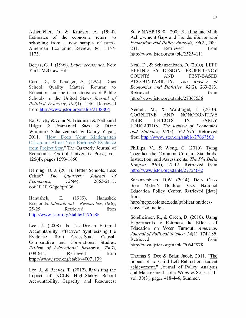
implementation process can be found in Table 1.
[Table 1 should be inserted about here]
Literature Review:
Although research has not yet been published about the switch to Common Core State
Standards and the effect of these new standards, there is a large body of evidence about the
transition to No Child Left Behind in the 2000s. Jacob (2005) examined Chicago Public Schools
and found that an accountability program caused math and reading scores to increase. Jacob uses
a difference in difference model which examines student achievement pre-accountability and
post-accountability program s in Chicago and other large Midwestern cities. Jacob found that
the scores increased on high-stakes exams but not low-stakes exams, which suggests that
teachers were teaching to the test, instead of the accountability program creating increased
learning.
Neal and Schanzenbach (2010) also examined the effects of accountability programs in
Chicago Public Schools. Neal and Schanzenbach examined the implementation of No Child Left
Behind and its effects on the distribution of changes in test scores. The authors use test scores
from pre and post accountability program to estimate the impact of No Child Left Behind on test
scores. They find that the implementation of No Child Left Behind increased the scores of
students near the proficiency cutoff, but does not affect students at the bottom or top of the
proficiency distribution.
Dee and Jacob (2009) examined the effect of NCLB on students and teachers; they find
that NCLB policies shift instructional time to math and reading from other subjects and increase
the share of teachers with graduate degrees. Although they concluded that there were
7
improvements in scores on high stakes tests, the authors attribute these improvements to
increasing teacher resources instead of NCLB policies.
Dee and Jacob again examined the effectiveness of No Child Left Behind in 2011 using
National Assessment of Educational Progress data. The authors used a comparative interrupted
time series analysis to compare the effects of No Child Left Behind in states that did not have
consequential accountability programs to states that did have significant accountability
programs, prior to the implementation of No Child Left Behind. They found that No Child Left
Behind increased the math scores for 4th graders and that the effect was especially evident in
traditionally low-performing groups, but that there were no gains in reading scores.
Lee and Reeves (2012) examined the effects of high-stakes accountability under NCLB.
They used National Assessment of Educational Progress Data to examine long run trends at the
state level to discern the effectiveness of No Child Left Behind. They also used a comparative
interrupted time series model in their analysis, but instead of examining states that had
accountability programs before No Child Left Behind as their comparison, they examined the
“fidelity and rigor” of No Child Left Behind implementation across states, and their proxy of
learning is the achievement gap for students in reading and math. They found that high-stakes
test scores improved concurrently with NCLB’s implementation, but scores on low-stakes tests--
such as the NAEP test-- did not improve markedly.
I use an ordinary least squares (OLS) model with control data instead of difference-in-
difference or time series model analysis, but these papers lay the foundation of analysis of
national education policy. I seek, like them, to examine the effectiveness of educational policy.
I use school-level test score data disaggregated by demographic subgroups and by to estimate the
effectiveness of Common Core State Standards on raising test scores. My paper is unique
because my dataset has a finer measure of a school’s transition to Common Core standards than
the binary pre/post implementation used by studies that examined No Child Left Behind. This
finer measure of implementation is more realistic to the way that a new program works in
schools, and will be better able to capture effects of implementation in my data set. I expect to
find that a higher level of Common Core State Standards implementation is associated with an
increase in test scores for students who are in historically underperforming subgroups, as Dee
and Jacob (2009) find, but little to no effect on higher performing groups.
8
Data:
I use data from California Public High Schools that indicates their level of
implementation of Common Core and provides information about their academic achievement
through end-of-year high-stakes test scores. I use public school data because Common Core
State Standards affected public schools. I focus on California because the California Department
of Education has collected data on the implementation of Common Core State Standards at a
district level.
Implementation data come from a voluntary survey of school districts in California,
which was implemented by the California Department of Education. 128 districts out of the 517
districts in California responded to this 30 question survey. Geographically, these districts cover
California evenly, with 23 in Southern California covering seven out of the seven counties, eight
in Central California covering six out of fifteen counties and 25 in Northern California covering
18 out of 36 of the counties. Since the survey was voluntary, I find that the intensity of
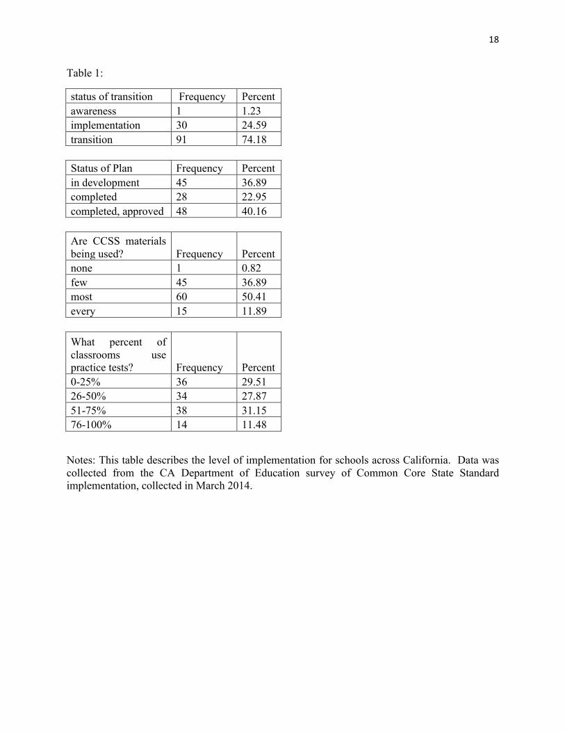
implementation into Common Core is not random. Each control is significantly correlated with
the measure of implementation, although with small magnitudes. The results of regressing the
measure of implementation against the controls, discussed below, can be found in Table 2.
[Insert Table 2]
We see that for the sum of encoded variables, which takes values from 0 to 10 and is a
measure of overall implementation, a one point increase in implementation is associated with a
lower unemployment rate, a slightly lower mean income, a lower percent of families in poverty,
and a lower English as a Second Language (ESL) population. A slightly lower mean income and
lower unemployment rate are counter-intuitive, because I expect these two measures to be
trending together. However, these two measures trending opposite can be interpreted as higher
common core implementation in middle-class counties and lower implementation in very high-
income and very low-income counties. This means that overall, schools that are further in the
implementation process have higher education spending, and are more English speaking and
middle class. This causes concern for bias in our estimates, and although I control for these
9
characteristics in our main regression specifications, the estimate of the effect of Common Core
State Standards may be overestimated.
The surveys asked several questions about the implementation of Common Core State
Standards. I pull four variables that describe the level of implementation from this survey: a
self-categorization of the districts into three levels of implementation, the status of the district’s
implementation plan, the degree of Common Core State Standards materials being used in
classrooms, and the level of practice tests being used in classrooms.
The level of implementation, from lowest to highest, is coded as “awareness,”
“transition,” and “implementation.” The status of a district’s plan is coded as “in development,”
“completed,” or “completed and approved.” The degree of Common Core State Standards
materials that are being used in classes is coded as “none”, “few”, “most” and “every”, and the
level of practice tests being used in classrooms is coded as “0-25%”, “26-50%”, “51-75%”, “76-
100%”. These percentages refer to the percentage of classrooms in the district that use practice
tests for the high-stakes standardized test at the end of the year.
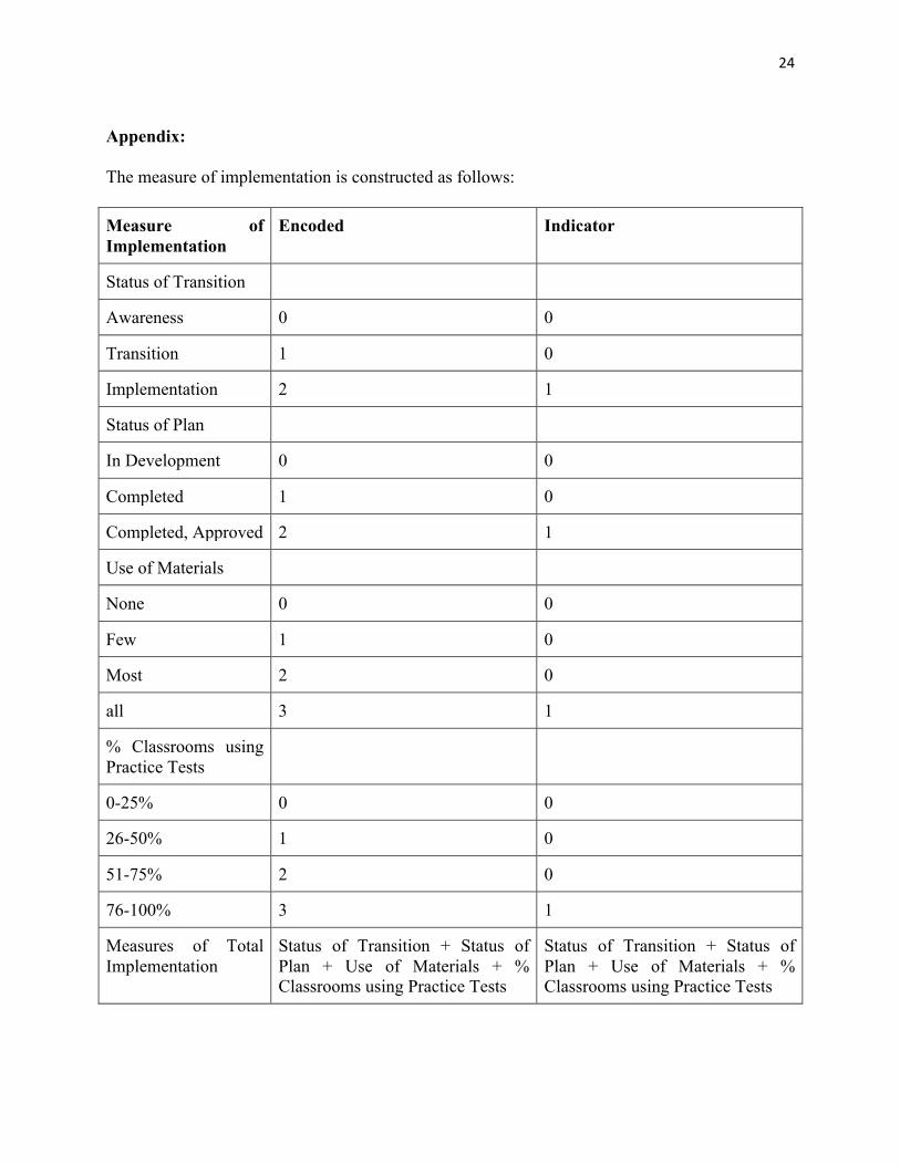
I also create two variables which are a summation of the indicator variables and the
encoded variables to capture an overall level of implementation for each school. Details about
the construction of these variables can be found in the appendix. In Table 1 you see a summary
of where schools are in the implementation process.
I collected two years of SBA scores, all the data currently available, from the high
schools in the 128 districts that responded to the implementation survey. SBA tests only 11th-
grade students at the high school level, so I use their scores in both math and English. These
scores are the average score for the students being tested at the grade level. The unit of
observation is at the school level. I have data for the whole population and subgroups, which
allows us to examine effects on different populations within the school. This allows us to
analyze the results for all of the 45 subgroups given in the data, but I report results for the whole
population of students , as well as six other subgroups, which are economically disadvantaged
students, Hispanic students, Hispanic and economically disadvantaged students, Hispanic and
not economically disadvantaged students, students whose parent’s highest level of education was
high school, and students whose parent’s highest level of education was a college degree. I
chose these subgroups because they have large enough sample sizes and because they showed
significant results.
10
I collected four years of STAR testing data for each of the high schools in the 128
districts that responded to the implementation survey, from testing year 2010 to 2013. STAR
testing was given to all students who were not on an Individualized Education Program (IEP).
STAR testing scores are the average score for all students in the testing group at each school.
While STAR testing covers Math, English Language Arts, Science, and History, I keep only the
ELA and Math scores because those are the only subjects covered by Common Core State
Standards and tested by Smarter Balanced Assessments. Every 11th grader takes the same
English Language Arts exam, but the math exams are tailored to the math class that the student is
currently enrolled in. As detailed in the Appendix, I combine the math scores to provide a single
observation for each subgroup at each school.
Individual year STAR scores for each school give a baseline achievement for the schools,
which will be compared to SBA testing. Both STAR and SBA testing scores are reported for all
students and are also broken down into subgroups. I focus on the subgroups of economically
disadvantaged students, Hispanic students, Hispanic and economically disadvantaged students,
Hispanic and not economically disadvantaged students, students whose parent’s highest level of
education was high school, and students whose parent’s highest level of education was a college
degree. I pick these subgroups because other than students whose parents have college degrees,
all of these subpopulations are traditionally underperforming minority subgroups. Most
literature about education uses black students are the minority group. Since I am using
California data, choosing Hispanic students as the minority group allowed for more observations
and is more descriptive of the current demographic patterns in California schools.
I also collected data about county demographics to control for the characteristics of the
school population. I collected the unemployment rate from the Bureau of Labor Statistics, which
was measured in 2010. From the 2010 census, I collected the percent of the population that is
black, white, Asian, American Indian/ Native American, Pacific Islander, and Hispanic. In the
Government census, which was also collected in 2010, I collected the amount of education
spending in each county of California. From the American Community Survey, I obtained the
mean income of each country, the percent of the population for which English is a Second
Language, and the percent of families in poverty, which is defined as the percent of households
with a child between the ages of 5 and 17 who is below the poverty line.
11
These variables will allow me to control for county characteristics in the regression in
order to create unbiased regression results. Economics of education literature finds that these
characteristics affect the education outcomes of students, so controlling for these characteristics
minimizes the omitted variable bias of my estimates.
Empirical Method:
In this paper, I seek to examine the effects of Common Core State Standards on
test scores. To do this, I use end-of-year high-stakes test scores to proxy learning and the
creation of human capital. The acquisition of human capital is the variable of interest, and many
researchers use test scores as a measure of learning (Dee and Jacob 2011, Jacob 2005, Neal and
Schanzenbach 2010, Lee 2008). Using test scores as the parameter of interest is not without
faults, but research has shown that increases in end-of-year test scores are mirrored in long-term
measures of human capital acquisition, such as a higher salary (Chetty et al, Schanzenbach).
This evidence, coupled with the short time that Common Core State Standards has been
implemented, makes using test scores the best option to proxy learning.
The variation across schools is the amount of implementation of Common Core State
Standards that has occurred. This is a treatment intensity analysis. To estimate the effects of
Common Core, I regress the post implementation test scores (SBA) against pre-implementation
test scores (STAR), the level of implementation, and controls.
I use two separate specifications to estimate the effects of the intensity of Common Core
on test scores: a small model and a large model.
The small model, model 1, is:
(scoreSBA)st = 𝛃(Common Core)st +𝛼(scoreSTAR) s(t-2) + 𝜺st
where s is the school, t is the year the test was taken in, and (t-2) is the STAR score of the
school prior to the passage of Common Core. This model estimates the effect of the
implementation of Common Core, while controlling for the school’s previous test score.
The large model, model 2, is:
(scoreSBA)st = 𝛼(scoreSTAR) s(t-2) + 𝛃(Common Core)st+ (controls)st + 𝜺st
where s is the school, t is the year the test was taken in, and (t-2) is the STAR score of the
school prior to the passage of Common Core and controls are the control variables discussed in
the data section as well as lagged STAR test scores from 2012 and 2011. Common Core is the
12
set of indicator and encoded variables that measure the implementation of Common Core across
four measures of implementation, as described in the data discussion. For each, the value of the
indicator is 1 if it is on the highest level of implementation and 0 otherwise.
We run this regression for all students and the selected subgroups to estimate the effect
on differentiated populations within schools. 𝛃 estimates the effect of the new Common Core
curriculum on test scores which are designed to measure student learning. 𝛃 is probably not
causal because the sample is not random. Educational economics is particularly susceptible to
omitted variable bias due to the number of variables which are very hard to measure and
quantify, such as natural intelligence, persistence, and family support of education at home, as
well variables that are not tracked well, such as socioeconomic status, amount of effort, and
teacher quality. All of these factors contribute to a student's’ academic achievement and could
cause a bias in our estimates of the effect of Common Core. I control for the effect of variables
that can be estimated, including the socioeconomic status of the area that the school is located in
and the quality of the school.
Results:
In this section, I examine the effects of implementation of Common Core on student’s
test scores. These results may not be causal because our sample of schools is not random.
However, I see significance in all measures, although of differing signs and magnitudes.
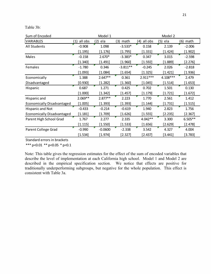
Overall Effect:
The sum of indicators and sum of encoded variables show the same trends, which can be
seen in Tables 3a and 3b. For all scores in the small model, I observe that there is a negative
sign but no statistical significance for the whole population of students. I also see that for all
students in the small model, the effect of common core on math scores is negative. In the
indicator model (3a) I see that the coefficient is -8.343, which can be interpreted as a one point
increase in implementation causes average math scores for the school to drop by 8.343 points.
The sum of indicator variables take the values 0 to 4. The average test score variable takes
values between 2492 and 2370, with a standard deviation of 46. So the 8.343 point effect is 0.18
of a standard deviation change. In the encoded model (3b) the effect is -3.533, which can be
interpreted as a one point increase in implementation causes average math scores for the school
to drop by 3.533 points. The encoded variable takes the values 0 to 10, so the effect is consistent
13
across the indicator and encoded models because of the differing range of the variables
associated with implementation. In the large model, I see a negative and significant effect on all
students’ scores with the indicator variable, but this effect is not statistically significant when the
encoded variable is used. This may be due to the differing ranges of the variables.
The large model for all observations (column 4) shows a positive and statistically
significant result for students whose parents highest level of education is high school. The effect
is similar in magnitude at 4.341 and 4.042 points. This can be interpreted as a one point increase
in the implementation of Common Core being associated with a 4 point increase in the overall
scores for those students. This estimate is consistent across the two estimates. I also see in the
large model (column 6) that an increase in implementation of Common Core is associated with a
6.505 and 6.918 point increase in math test scores for the large model for students whose
parent’s highest level of education was high school.
The overall effect for all students was negative, but for students whose parents highest
level of education was high school the effect was positive and statistically significant in the large
model for both overall scores and math scores.
[Inset Tables 3a and 3b]
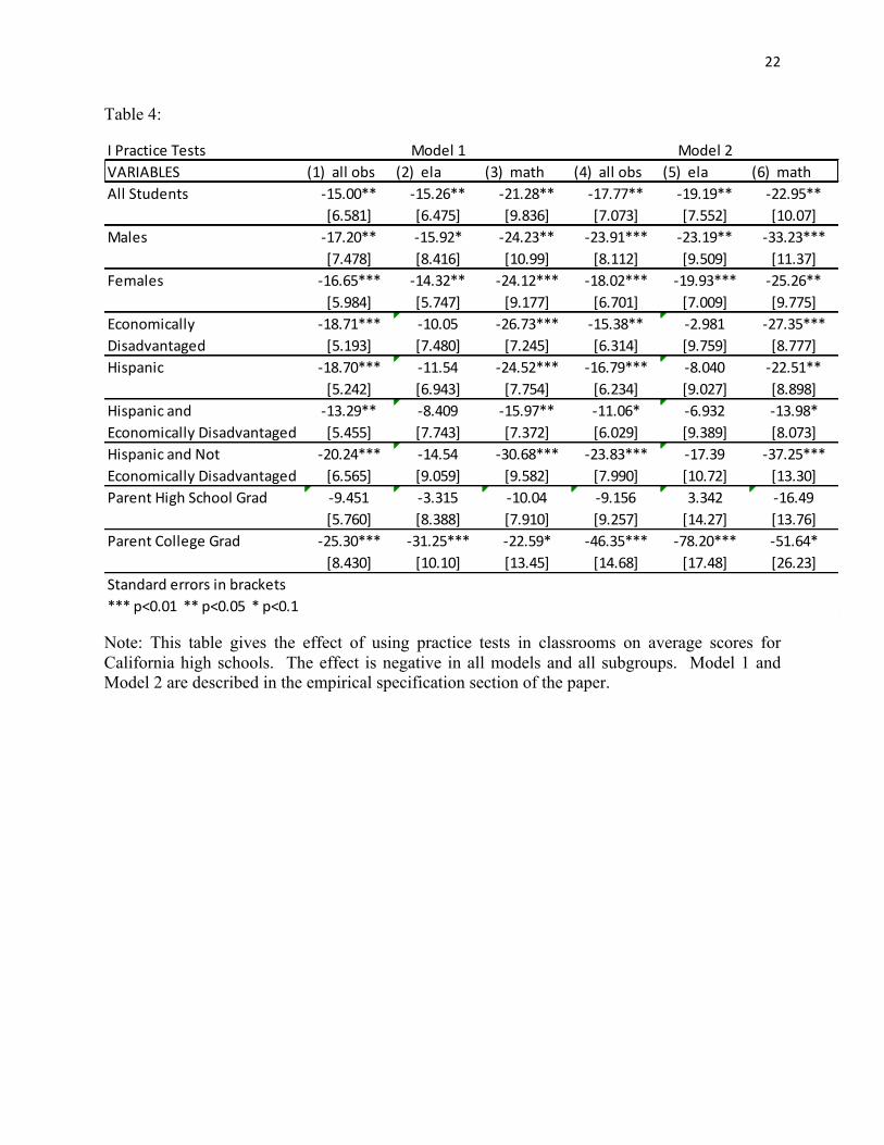
Effect of Practice Tests:
Next, I examine the effect of practice tests; the effect is negative when the effect is
significant. The results can be found in Table 4. The effect is not significant for students whose
parent’s highest level of education is high school, which may explain the overall positive
significance of that subgroup. Overall, the coefficients are larger than the coefficients that were
observed in the overall effects.
In the small model, Column 1 of Table 4, I see that the effects on overall test scores are
negative and statistically significant for all subgroups except for students whose parents highest
level of education is high school. These effects are between 13 and 25 points, or about ¼ to ½ of
a standard deviation. This means that a school that is using practice tests in 76-100% percent of
its classrooms has average scores 13 to 25 points lower than schools which are not at the highest
level of implementation. The change in average scores is both significant and large in
magnitude. These effects persist in the large model which includes controls, and the effect is
14
similar in magnitude. I see, for example, that Hispanic students whose schools are using practice
tests in 76-100% of classrooms have an average score that is 16.79 points lower than a cohort of
Hispanic students who were at a school that did not use practice tests. We see this trend
replicated in the math scores for both the small and large models, where the effect is negative
and statistically significant for all groups. The English Language Arts scores are also negative,
but are not significant for economically disadvantaged students, Hispanic students overall, or
either set of economic subgroups of Hispanic students.
There are several reasons that this negative trend could be occurring, and I will propose
two explanations. Both explanations hinge on the fact that when a teacher allocates time to
practice tests or a district mandates a certain amount of time allocated to practice tests,
instructional time is not being spent on actual learning and human capital formation.
The first explanation is that the practice test being utilized in classrooms are not good at
preparing students for taking the smarter balanced assessments. It is possible that there is not
enough computer time available to schools to take computer-based practice tests, and so pencil
and paper practice tests are being used, even though this is not the mode that the smarter
balanced tests are given in. This would make the practice tests less efficient in helping raise
students’ scores on the real test. In this scenario, the practice tests are diverting time away from
real learning while at the same time not effectively teaching the students how to take the new
tests.
The second explanation is that the smarter balanced assessments are excellent at
measuring actual learning and human capital formation. Therefore, any instructional time
allocated away from learning will always be a misallocation. Common Core attempts to teach
critical thinking and problem solving along with more traditional math and English Language
Arts topics, and smarter balanced assessments attempts to test for these skills as well. So if the
smarter balanced assessments are successfully testing for critical thinking or problem-solving, it
is possible that practice tests cannot be formulated to practice these skills more effectively than
teaching the skills outside of practice tests.
To test which of these explanations is correct, or if another explanation is true, more
years of data and more specific data about what practice tests are being used is needed.
[Insert Table 4]
15
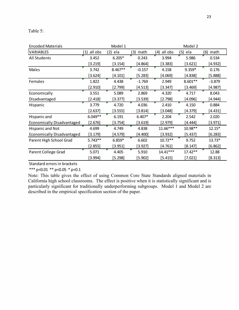
Effect of Common Core Materials:
Next, I examine the effect of using materials designed to align with the Common Core
curriculum on student’s scores. Because Common Core State Standards are standardizing the
topics taught in each school, the amount of Common Core aligned materials may be the best
measure of how effective Common Core State Standards will be long term. The results can be
found in Table 5.
We conclude that for all students, the only significant result is a positive effect in the
small model on English Language Arts scores. This effect is still positive in the large model but
is no longer statistically significant. For students that are Hispanic and economically
disadvantaged I find positive and significant effects for test scores overall and in math
specifically in the small model, but these effects also fade in the larger model, although the effect
continues to be positive.
For students that are Hispanic and not economically disadvantaged, I find that the effect
of using Common Core-aligned materials is positive and significant for all scores and math and
English Language Arts individually in the large model. Their effects are not as large in
magnitude as effects in practice tests but are between a quarter and a third of a standard
deviation, which is significant in education scores.
For students whose parent’s highest level of education is high school the effect of using
Common Core-aligned materials is positive in the small model for all test scores and English
Language Arts specifically, and in the large model for scores overall and in math specifically.
Students parent’s level of education is a factor that predicts student’s success, with students
whose parents have more school performing better than their peers whose parents completed less
school, so the positive effect of materials is important for this subgroup in increasing their
achievement and limiting disaprities.
Students whose parent’s highest level of education is college also show significant
positive results in the large model for all scores and English Language Arts scores. These effects
show that Common Core materials are effective in raising test scores for students who are in
traditionally high performing subgroups as well as historically low-performing subgroups.
[Insert Table 5]
16
Conclusion:
The goal of this paper was to examine the effect of Common Core implementation on test
scores in California high schools. I found that overall test scores were significantly affected by
the amount of implementation of Common Core in the school in a positive direction, but the
effects were small in magnitude. The small magnitude was driven by large negative effects
created by practice tests counterbalanced by positive effects created by use of Common Core-
aligned materials. For certain subgroups, especially economically disadvantaged students, and
minority students, test scores were strongly influenced by Common Core implementation.
This evidence matches with the results that I expected to find based on literature about
school accountability programs. Low performing schools and subgroups benefited from the
creation of standards, whereas high performing schools did not benefit from the standards. One
possible explanation for this is that high performing schools did not have very much room for
improvement-- their average scores were already very high, so there was little room to raise
scores. In this case, I do not expect for standards programs to increase scores because no
improvement is needed in those schools. On the other hand, schools that need help and are
underperforming will benefit from standards, because schools will make adjustments to teaching
styles, reallocate instructional time, or make other changes to the structure of the school in order
to meet those standards.
Common Core State Standards should continue to be examined for effectiveness. While
my results show positive effects of Common Core, as more data becomes available researchers
should verify these results. Researchers should investigate the effects of practice tests as more
data and more years of data are available in order to create more effective practice tests or, if
practice tests continue to prove ineffective, provide guidance to teachers on more efficient
allocation of time and resources in the classroom. In addition, future researchers will be able to
find natural experiments to grow the body of evidence for Common Core State Standards. In
particular, the decoupling of federal funding from the adoption of Common Core State Standards
that occurred in the ESSA may create natural experiments with states repealing or not adopting
the standards.
17
Ashenfelter, O. & Krueger, A. (1994). Estimates of the economic return to schooling from a new sample of twins. American Economic Review, 84, 1157-1173. Borjas, G. J. (1996). Labor economics. New York: McGraw-Hill. Card, D., & Krueger, A. (1992). Does School Quality Matter? Returns to Education and the Characteristics of Public Schools in the United States. Journal of Political Economy, 100(1), 1-40. Retrieved from http://www.jstor.org/stable/2138804 Raj Chetty & John N. Friedman & Nathaniel Hilger & Emmanuel Saez & Diane Whitmore Schanzenbach & Danny Yagan, 2011. "How Does Your Kindergarten Classroom Affect Your Earnings? Evidence from Project Star," The Quarterly Journal of Economics, Oxford University Press, vol. 126(4), pages 1593-1660. Deming, D. J. (2011). Better Schools, Less Crime? The Quarterly Journal of Economics, 126(4), 2063-2115. doi:10.1093/qje/qjr036 Hanushek, E. (1989). Hanushek Responds. Educational Researcher, 18(6), 25-25. Retrieved from http://www.jstor.org/stable/1176186 Lee, J. (2008). Is Test-Driven External Accountability Effective? Synthesizing the Evidence from Cross-State Causal-Comparative and Correlational Studies. Review of Educational Research, 78(3), 608-644. Retrieved from http://www.jstor.org/stable/40071139 Lee, J., & Reeves, T. (2012). Revisiting the Impact of NCLB High-Stakes School Accountability, Capacity, and Resources:
State NAEP 1990—2009 Reading and Math Achievement Gaps and Trends. Educational Evaluation and Policy Analysis, 34(2), 209-231. Retrieved from http://www.jstor.org/stable/23254111 Neal, D., & Schanzenbach, D. (2010). LEFT BEHIND BY DESIGN: PROFICIENCY COUNTS AND TEST-BASED ACCOUNTABILITY. The Review of Economics and Statistics, 92(2), 263-283. Retrieved from http://www.jstor.org/stable/27867536 Neidell, M., & Waldfogel, J. (2010). COGNITIVE AND NONCOGNITIVE PEER EFFECTS IN EARLY EDUCATION. The Review of Economics and Statistics, 92(3), 562-576. Retrieved from http://www.jstor.org/stable/27867560 Phillips, V., & Wong, C. (2010). Tying Together the Common Core of Standards, Instruction, and Assessments. The Phi Delta Kappan, 91(5), 37-42. Retrieved from http://www.jstor.org/stable/27755642
Schanzenbach, D.W. (2014). Does Class Size Matter? Boulder, CO: National Education Policy Center. Retrieved [date] from http://nepc.colorado.edu/publication/does-class-size-matter.
Sondheimer, R., & Green, D. (2010). Using Experiments to Estimate the Effects of Education on Voter Turnout. American Journal of Political Science, 54(1), 174-189. Retrieved from http://www.jstor.org/stable/20647978 Thomas S. Dee & Brian Jacob, 2011. "The impact of no Child Left Behind on student achievement," Journal of Policy Analysis and Management, John Wiley & Sons, Ltd., vol. 30(3), pages 418-446, Summer.
18
Table 1:
status of transition Frequency Percent awareness 1 1.23 implementation 30 24.59 transition 91 74.18 Status of Plan Frequency Percent in development 45 36.89 completed 28 22.95 completed, approved 48 40.16 Are CCSS materials being used? Frequency Percent none 1 0.82 few 45 36.89 most 60 50.41 every 15 11.89 What percent of classrooms use practice tests? Frequency Percent 0-25% 36 29.51 26-50% 34 27.87 51-75% 38 31.15 76-100% 14 11.48
Notes: This table describes the level of implementation for schools across California. Data was collected from the CA Department of Education survey of Common Core State Standard implementation, collected in March 2014.
19
VARIAB
LES
Indiacator
status of
transition
Encode
d status of
transition
Indiacator
status of p
lan
Encode
d Status of P
lan
Indiacator
Common
Co
re
Encode
d Co
mmon
Co
re
Indiacator
practice tests
Encode
d practice tests
Sum on
Encode
dSum of
Indicators
unem
ploymen
trate
0.00914
0.00271
-‐0.0547**
-‐0.117***
-‐0.0560***
-‐0.0904***
0.00917
0.0538
-‐0.151*
-‐0.0923**
[0.0202]
[0.0219]
[0.0240]
[0.0419]
[0.0151]
[0.0328]
[0.0159]
[0.0497]
[0.0882]
[0.0442]
meanincom
e-‐1.17e-‐05*
-‐1.64e-‐05**
-‐3.57e-‐05***
-‐5.02e-‐05***
-‐2.72e-‐07
-‐1.02e-‐05
-‐1.67e-‐05***
-‐2.48e-‐05
-‐0.000102***
-‐6.43e-‐05***
[7.04e-‐06]
[7.93e-‐06]
[8.34e-‐06]
[1.52e-‐05]
[5.27e-‐06]
[1.19e-‐05]
[5.55e-‐06]
[1.80e-‐05]
[3.19e-‐05]
[1.54e-‐05]
faminpo
verty
-‐0.0540***
-‐0.0587***
-‐0.0858***
-‐0.161***
0.0167
0.0393
-‐0.0449***
-‐0.0289
-‐0.210***
-‐0.168***
[0.0155]
[0.0174]
[0.0184]
[0.0333]
[0.0116]
[0.0261]
[0.0122]
[0.0395]
[0.0701]
[0.0339]
lned
uspe
nding
0.158***
0.0649
0.160***
0.0940
-‐0.128***
-‐0.221***
0.0986***
0.247**
0.185
0.288***
[0.0458]
[0.0444]
[0.0543]
[0.0849]
[0.0343]
[0.0664]
[0.0361]
[0.101]
[0.179]
[0.100]
whitepo
p-‐0.0199
-‐0.0113
0.00441
-‐0.0765
0.151***
0.205***
-‐0.0936***
-‐0.240***
-‐0.123
0.0424
[0.0252]
[0.0281]
[0.0298]
[0.0537]
[0.0188]
[0.0420]
[0.0198]
[0.0636]
[0.113]
[0.0550]
blackpop
-‐0.0333
-‐0.0184
-‐0.0448
-‐0.152**
0.175***
0.197***
-‐0.165***
-‐0.376***
-‐0.350**
-‐0.0682
[0.0332]
[0.0370]
[0.0394]
[0.0706]
[0.0249]
[0.0553]
[0.0262]
[0.0837]
[0.149]
[0.0726]
indianpo
p0.0837
0.0371
-‐0.0310
-‐0.153
0.127***
-‐0.129
-‐0.173***
-‐0.794***
-‐1.039***
0.00757
[0.0543]
[0.0609]
[0.0642]
[0.116]
[0.0406]
[0.0911]
[0.0427]
[0.138]
[0.245]
[0.118]
asianp
op0.000333
0.0157
0.0183
-‐0.0819
0.199***
0.285***
-‐0.0857***
-‐0.280***
-‐0.0613
0.132*
[0.0327]
[0.0366]
[0.0387]
[0.0700]
[0.0245]
[0.0548]
[0.0257]
[0.0830]
[0.147]
[0.0714]
hisppo
p0.0319**
0.0370**
0.0296*
0.0135
0.106***
0.151***
-‐0.0320***
-‐0.135***
0.0658
0.136***
[0.0147]
[0.0165]
[0.0174]
[0.0315]
[0.0110]
[0.0246]
[0.0116]
[0.0373]
[0.0662]
[0.0321]
eslpop
-‐0.0374***
-‐0.0309***
-‐0.0205**
-‐0.0139
-‐0.0328***
-‐0.0542***
-‐0.00598
0.0253
-‐0.0738**
-‐0.0966***
[0.00769]
[0.00854]
[0.00910]
[0.0163]
[0.00575]
[0.0128]
[0.00606]
[0.0193]
[0.0343]
[0.0168]
Observations
244
246
244
246
244
246
244
246
246
244
R-‐squared
0.343
0.278
0.290
0.267
0.349
0.264
0.256
0.213
0.307
0.441
Standard erro
rs in brackets
*** p
<0.01, **
p<0.05, * p<0.1
Table 2:
Notes: This table gives the results from
regressing
con
trol variables on measures o
f implem
entatio
n of com
mon
core. Con
trol
varia
bles were collected
from
the Am
erican
Com
mun
ity Survey, 201
0 Ce
nsus, and
Bureau of Lab
or Statistics
20
Table 3a:
Note: This table gives the regression estimates for the effect of the sum of indicator variables that describe the level of implementation at each California high school. Model 1 and Model 2 are described in the empirical specification section. We notice that effects are positive for traditionally underperforming subgroups, but negative for the whole population.
Sum of Indicators VARIABLES (1) all obs (2) ela (3) math (4) all obs (5) ela (6) mathAll Students -‐3.166 -‐0.150 -‐8.343*** -‐3.616* -‐0.926 -‐8.319***
[2.097] [2.098] [3.108] [2.093] [2.087] [3.115]Males -‐1.209 1.889 -‐5.996* -‐1.794 0.997 -‐6.889**
[2.321] [2.655] [3.358] [2.336] [2.715] [3.298]Females -‐2.970 -‐0.723 -‐6.507** -‐3.030 -‐1.034 -‐6.638**
[1.837] [1.798] [2.815] [1.854] [1.815] [2.841]Economically 0.965 3.434 -‐1.528 0.378 2.693 -‐2.036Disadvantaged [1.553] [2.138] [2.312] [1.571] [2.232] [2.318]Hispanic 1.770 2.182 1.474 1.073 2.016 0.293
[1.643] [2.170] [2.444] [1.591] [2.243] [2.313]Hispanic and 1.437 2.887 2.771 0.383 1.255 1.575Economically Disadvantaged [1.735] [2.456] [2.447] [1.662] [2.504] [2.429]Hispanic and Not 0.556 -‐0.222 1.701 1.517 0.435 2.732Economically Disadvantaged [2.048] [2.956] [2.810] [1.944] [2.551] [2.870]Parent High School Grad 4.169** 6.168** 5.321* 4.341** 6.516** 6.918**
[1.846] [2.418] [2.698] [1.842] [2.393] [2.890]Parent College Grad -‐1.898 -‐2.593 -‐1.868 -‐3.061 -‐4.816 -‐1.749
[2.711] [3.603] [4.005] [2.655] [3.368] [3.926]Standard errors in brackets*** p<0.01 ** p<0.05 * p<0.1
Model 1 Model 2
21
Table 3b:
Note: This table gives the regression estimates for the effect of the sum of encoded variables that describe the level of implementation at each California high school. Model 1 and Model 2 are described in the empirical specification section. We notice that effects are positive for traditionally underperforming subgroups, but negative for the whole population. This effect is consistent with Table 3a.
Sum of EncodedVARIABLES (1) all obs (2) ela (3) math (4) all obs (5) ela (6) mathAll Students -‐0.908 1.098 -‐3.533* 0.158 2.139 -‐2.006
[1.195] [1.176] [1.795] [1.331] [1.424] [1.902]Males -‐0.158 2.670* -‐3.383* 0.347 3.015 -‐2.598
[1.340] [1.491] [1.960] [1.592] [1.889] [2.276]Females -‐1.780 0.346 -‐3.811** -‐0.245 2.026 -‐2.818
[1.093] [1.084] [1.654] [1.325] [1.421] [1.936]Economically 1.388 2.647** 0.361 2.911*** 4.108*** 2.479Disadvantaged [0.930] [1.282] [1.360] [1.045] [1.514] [1.653]Hispanic 0.687 1.271 0.425 0.702 1.501 0.130
[1.000] [1.342] [1.457] [1.179] [1.721] [1.672]Hispanic and 2.069** 2.877** 2.223 1.770 2.561 1.412Economically Disadvantaged [1.005] [1.393] [1.393] [1.144] [1.731] [1.515]Hispanic and Not -‐0.433 -‐0.214 -‐0.619 1.940 2.823 1.756Economically Disadvantaged [1.181] [1.709] [1.626] [1.555] [2.235] [2.367]Parent High School Grad 1.767 2.277 2.335 4.042** 3.300 6.505**
[1.115] [1.550] [1.533] [1.656] [2.629] [2.478]Parent College Grad -‐0.990 -‐0.0600 -‐2.338 3.542 4.327 4.004
[1.534] [1.974] [2.327] [2.437] [3.441] [3.783]Standard errors in brackets*** p<0.01 ** p<0.05 * p<0.1
Model 1 Model 2
22
Table 4:
Note: This table gives the effect of using practice tests in classrooms on average scores for California high schools. The effect is negative in all models and all subgroups. Model 1 and Model 2 are described in the empirical specification section of the paper.
I Practice TestsVARIABLES (1) all obs (2) ela (3) math (4) all obs (5) ela (6) mathAll Students -‐15.00** -‐15.26** -‐21.28** -‐17.77** -‐19.19** -‐22.95**
[6.581] [6.475] [9.836] [7.073] [7.552] [10.07]Males -‐17.20** -‐15.92* -‐24.23** -‐23.91*** -‐23.19** -‐33.23***
[7.478] [8.416] [10.99] [8.112] [9.509] [11.37]Females -‐16.65*** -‐14.32** -‐24.12*** -‐18.02*** -‐19.93*** -‐25.26**
[5.984] [5.747] [9.177] [6.701] [7.009] [9.775]Economically -‐18.71*** -‐10.05 -‐26.73*** -‐15.38** -‐2.981 -‐27.35***Disadvantaged [5.193] [7.480] [7.245] [6.314] [9.759] [8.777]Hispanic -‐18.70*** -‐11.54 -‐24.52*** -‐16.79*** -‐8.040 -‐22.51**
[5.242] [6.943] [7.754] [6.234] [9.027] [8.898]Hispanic and -‐13.29** -‐8.409 -‐15.97** -‐11.06* -‐6.932 -‐13.98*Economically Disadvantaged [5.455] [7.743] [7.372] [6.029] [9.389] [8.073]Hispanic and Not -‐20.24*** -‐14.54 -‐30.68*** -‐23.83*** -‐17.39 -‐37.25***Economically Disadvantaged [6.565] [9.059] [9.582] [7.990] [10.72] [13.30]Parent High School Grad -‐9.451 -‐3.315 -‐10.04 -‐9.156 3.342 -‐16.49
[5.760] [8.388] [7.910] [9.257] [14.27] [13.76]Parent College Grad -‐25.30*** -‐31.25*** -‐22.59* -‐46.35*** -‐78.20*** -‐51.64*
[8.430] [10.10] [13.45] [14.68] [17.48] [26.23]Standard errors in brackets*** p<0.01 ** p<0.05 * p<0.1
Model 1 Model 2
23
Table 5:
Note: This table gives the effect of using Common Core State Standards aligned materials in California high school classrooms. The effect is positive when it is statistically significant and is particularly significant for traditionally underperforming subgroups. Model 1 and Model 2 are described in the empirical specification section of the paper.
Encoded MaterialsVARIABLES (1) all obs (2) ela (3) math (4) all obs (5) ela (6) mathAll Students 3.452 6.205* 0.243 3.994 5.986 0.534
[3.219] [3.154] [4.864] [3.383] [3.621] [4.932]Males 3.742 8.467** -‐0.157 4.158 9.359* 0.176
[3.624] [4.101] [5.283] [4.069] [4.838] [5.888]Females 1.822 4.438 -‐1.769 2.949 8.601** -‐3.879
[2.910] [2.799] [4.513] [3.347] [3.469] [4.987]Economically 3.551 5.089 2.869 4.320 4.717 8.043Disadvantaged [2.418] [3.377] [3.539] [2.798] [4.096] [4.944]Hispanic 3.779 4.720 4.036 2.410 4.150 0.884
[2.637] [3.555] [3.814] [3.048] [4.379] [4.431]Hispanic and 6.049** 6.191 6.407* 2.204 2.542 2.020Economically Disadvantaged [2.676] [3.754] [3.619] [2.979] [4.444] [3.971]Hispanic and Not 4.699 4.749 4.838 11.66*** 10.98** 12.15*Economically Disadvantaged [3.179] [4.579] [4.400] [3.932] [5.437] [6.283]Parent High School Grad 5.743** 6.859* 6.602 10.72** 9.752 13.73*
[2.855] [3.951] [3.927] [4.761] [8.147] [6.862]Parent College Grad 5.071 4.405 5.910 14.41*** 17.42** 12.88
[3.994] [5.298] [5.902] [5.415] [7.021] [8.313]Standard errors in brackets*** p<0.01 ** p<0.05 * p<0.1
Model 1 Model 2
24
Appendix: The measure of implementation is constructed as follows: Measure of Implementation
Encoded Indicator
Status of Transition
Awareness 0 0
Transition 1 0
Implementation 2 1
Status of Plan
In Development 0 0
Completed 1 0
Completed, Approved 2 1
Use of Materials
None 0 0
Few 1 0
Most 2 0
all 3 1
% Classrooms using Practice Tests
0-25% 0 0
26-50% 1 0
51-75% 2 0
76-100% 3 1
Measures of Total Implementation
Status of Transition + Status of Plan + Use of Materials + % Classrooms using Practice Tests
Status of Transition + Status of Plan + Use of Materials + % Classrooms using Practice Tests
25
Construction of the math scores for STAR testing: Students, depending on what math class they were enrolled in, took one of the following tests:
• Algebra I • Geometry • Algebra II • Integrated Mathematics 1 • Integrated Mathematics 2 • Integrated Mathematics 3 • Summative High School Mathematics
To analyze the data, I collapse the 7 tests into a single math test. The scores are averaged to
achieve a single math score.