Embed Size (px)
Citation preview

Electromagnetic Field Theory
Dr. Sandeep Nagar
G. D. Goenka University
November 23, 2015
Dr. Sandeep Nagar (G. D. Goenka University) Electromagnetic Field Theory November 23, 2015 1 / 349

Reference
The contents for the course has been prepared from the book:Principles of Electromagnetic6th edition Matthew N.O. Sadiku, S. V. KulkarniOxford University PressISBN - 9780199461851Students are advised to consult this or any other book for betterunderstanding of the subject.
Dr. Sandeep Nagar (G. D. Goenka University) Electromagnetic Field Theory November 23, 2015 2 / 349

Syllabus
Cartesian coordinates
cylindrical coordinates
Spherical coordinates
Vector calculus
Differential length, area and volume
Line, surface and volume integrals
Curl
Gradient
Divergence
Laplacian operators
Divergence theorem
Stokes theorem,
Greens Theorem
Dr. Sandeep Nagar (G. D. Goenka University) Electromagnetic Field Theory November 23, 2015 3 / 349

Basics of vector calculus
Revise the basics of vector calculus with topics
Definition of vector
Addition and subtraction of vectors
Dot and cross product
Dr. Sandeep Nagar (G. D. Goenka University) Electromagnetic Field Theory November 23, 2015 4 / 349

Coordinate system
Cartesian coordinates
Cylindrical coordinates
Spherical coordinates
Dr. Sandeep Nagar (G. D. Goenka University) Electromagnetic Field Theory November 23, 2015 5 / 349

Differential length, area and volume
NEED:
While solving physical problems, especially in conditions whennon-uniformity is an issue, small pieces of length, surface and/orvolume can be defined where uniformity can be safely assumed.
Vectors usually direct towards a point in space rather than a bigpiece of line, surface or volume.
Dr. Sandeep Nagar (G. D. Goenka University) Electromagnetic Field Theory November 23, 2015 6 / 349

Differential Length, Surface, Area
Length is usually associated as displacement in physical terms.
Differential displacement, surface and volume in cartesian coordinatesare shown in Fig. 7
Figure: Differential elements in cartesian coordinates
Dr. Sandeep Nagar (G. D. Goenka University) Electromagnetic Field Theory November 23, 2015 7 / 349

Differential Length, Surface, Area
~dl = dx ~ax + dy ~ay + dz ~az (1)
~dSx = dy .dz . ~ax (2)~dSy = dz .dx . ~ay (3)
~dSz = dx .dy . ~az (4)
dv = dx .dy .dz (5)
~dl and ~dS are vectors while dv is a scalarGeneral definition of surface element
~dS = dS . ~an
where:dS is area of surface element~an is unit vector normal to surface dS which directed away from thesurface (if surface is part of the volume, ~an points away from the). SeeFigure 7.
Dr. Sandeep Nagar (G. D. Goenka University) Electromagnetic Field Theory November 23, 2015 8 / 349

Differential Length, Surface, Area
In figure 7, area of surface ABCD and PQRS will be same (same dS)value but opposite in direction.
The two areas will be:
~dSABCD = dy .dz . ~ax
and~dSPQRS = −dy .dz . ~ax
because ~dSABCD grown towards positive x-axis and ~dSPQRS growstowards negative x-axis
Dr. Sandeep Nagar (G. D. Goenka University) Electromagnetic Field Theory November 23, 2015 9 / 349

Differential Length, Surface, Area in cylindrical coordinates
Figure: Differential elements in cylindrical coordinates
Dr. Sandeep Nagar (G. D. Goenka University) Electromagnetic Field Theory November 23, 2015 10 / 349

Differential Length, Surface, Area in cylindrical coordinates
~dl = d .ρ. ~aρ + ρ.dφ. ~aφ + dz . ~az (6)
~dSρ = ρ.dφ.dz . ~aρ (7)
~dSφ = dρ.dz . ~aφ (8)
~dSz = ρ.dφ.dρ. ~az (9)
dv = ρ.dρ.dφ.dz (10)
Dr. Sandeep Nagar (G. D. Goenka University) Electromagnetic Field Theory November 23, 2015 11 / 349

Differential Length, Surface, Area in spherical coordinates
Figure: Differential elements in spherical coordinates
Dr. Sandeep Nagar (G. D. Goenka University) Electromagnetic Field Theory November 23, 2015 12 / 349

Differential Length, Surface, Area in cylindrical coordinates
~dl = dr .~ar + r .dθ.~aθ + r .sinθ.dφ. ~aφ (11)
~dSr = r2.sinθ.dθ.dφ.~ar (12)~dSθ = r .sinθ.dr .dφ.~aθ (13)
~dSφ = r .dr .dθ. ~aφ (14)
dv = r2.sinθ.dr .dθ.dφ (15)
Dr. Sandeep Nagar (G. D. Goenka University) Electromagnetic Field Theory November 23, 2015 13 / 349

Line, surface and volume integrals
By a line we mean a path along a curve in space (1D movement)
By a surface we mean a 2D surface in space
By a volume we mean a 3D volume in space
A line integral of vector field ~A around a curve L is given by∫L
~A.d~l =
∫ b
a|~A|cosθ.dl
where line L starts from a and ends at b and θ is the angle between ~A anddifferential length d~l
Dr. Sandeep Nagar (G. D. Goenka University) Electromagnetic Field Theory November 23, 2015 14 / 349

Line Integral
Circulation of ~A around L is shown by integration for a closed loopdepicted by: ∮
L
~A.d~l
Figure: Line integralDr. Sandeep Nagar (G. D. Goenka University) Electromagnetic Field Theory November 23, 2015 15 / 349

Surface Integral
Surface Integral
ψ =
∫S
~A. ~andS =
∫S
~A.d ~S (16)
Figure: Surface integral
Dr. Sandeep Nagar (G. D. Goenka University) Electromagnetic Field Theory November 23, 2015 16 / 349

Closed Surface Integral
A closed surface encloses a volume
A closed surface integral is shown by:
ψ =
∮S
~A.d ~S
Physicaly, it signifies net outward flux
Dr. Sandeep Nagar (G. D. Goenka University) Electromagnetic Field Theory November 23, 2015 17 / 349

Volume integral
Volume integral of a
V =
∫vρvdv
Its important to note that both ρv as well as dv are scalar quantifies.
Dr. Sandeep Nagar (G. D. Goenka University) Electromagnetic Field Theory November 23, 2015 18 / 349

Del/ Gradient Operator in cartesian coordinates
∇ symbol signifies the del / gradient operator
∇ =∂
dx~ax +
∂
dy~ay +
∂
dz~az
Gradient operator operates on a scalar and produces a vector.
~∇V Gradient of scalar V~∇2V Laplacian of scalar V~∇. ~A Divergence of vector ~A~∇× ~A Curl of vector ~A
Dr. Sandeep Nagar (G. D. Goenka University) Electromagnetic Field Theory November 23, 2015 19 / 349

Gradient operator in cylindrical coordinates
Since ρ =√
x2 + y2 and tanφ = yx hence:
∂
∂x= cosφ
∂
∂ρ− sinφ
ρ
∂
∂φ(17)
∂
∂y= sinφ
∂
∂ρ+
cosφ
ρ
∂
∂φ(18)
Which yields ~∇ operator in cylindrical coordinates as:
~∇ = ~aρ∂
∂ρ+ ~aφ
1
ρ
∂
∂φ+ ~az
∂
∂z(19)
Dr. Sandeep Nagar (G. D. Goenka University) Electromagnetic Field Theory November 23, 2015 20 / 349

Gradient Operator for speherical coordinates
Find out gradient operator for speherical coordinates when we know that:
ρ =√x2 + y2 + z2
and
tanφ =
√x2 + y2
z
Dr. Sandeep Nagar (G. D. Goenka University) Electromagnetic Field Theory November 23, 2015 21 / 349

Gradient Operator for speherical coordinates
∂
∂x= sinθcosφ
∂
∂r+
cosθcosφ
r
∂
∂θ− sinφ
ρ
∂
∂φ(20)
Dr. Sandeep Nagar (G. D. Goenka University) Electromagnetic Field Theory November 23, 2015 22 / 349

Gradient Operator for speherical coordinates
∂
∂y= sinθsinφ
∂
∂r+
cosθsinφ
r
∂
∂θ− cosφ
ρ
∂
∂φ(21)
Dr. Sandeep Nagar (G. D. Goenka University) Electromagnetic Field Theory November 23, 2015 23 / 349

Gradient Operator for speherical coordinates
∂
∂z= cosθ
∂
∂r− sinθ
r
∂
∂θ(22)
Dr. Sandeep Nagar (G. D. Goenka University) Electromagnetic Field Theory November 23, 2015 24 / 349

Gradient Operator for speherical coordinates
~∇ = ~ar∂
∂r+ ~aθ
1
r
∂
∂θ+ ~aφ
1
r .sinθ
∂
∂r(23)
Dr. Sandeep Nagar (G. D. Goenka University) Electromagnetic Field Theory November 23, 2015 25 / 349

Gradient
Gradient (~∇) is used to find the direction of rate of change of a scalarfield
Mathematical meaning:Consider two points P1 and P2in space where contours V1,V2 and V3 aredefined.
Figure: Gradient of a scalar fieldDr. Sandeep Nagar (G. D. Goenka University) Electromagnetic Field Theory November 23, 2015 26 / 349

Gradient
dV =∂V
∂xdx +
∂V
∂ydy +
∂V
∂zdz (24)
dV = (∂V
∂x~ax +
∂V
∂y~ay +
∂V
∂z~az).(dx ~axdy ~ay + dz ~az) (25)
If:
~G = (∂V
∂x~ax +
∂V
∂y~ay +
∂V
∂z~az) (26)
Then:
dV = ~G .d~l = Gcosθdl (27)
dV
dl= Gcosθ (28)
Dr. Sandeep Nagar (G. D. Goenka University) Electromagnetic Field Theory November 23, 2015 27 / 349

Gradient
G = ~∇V =dV
dl|max =
dV
dn
where θ = 900 i.e. dVdn is normal derivative
Direction of G = ~∇V is that of maximum rate of change of fieldmagnitude~∇V is defined in same cartesian coordinate system as the definition
of scalar field V
Dr. Sandeep Nagar (G. D. Goenka University) Electromagnetic Field Theory November 23, 2015 28 / 349

Gradient operator in different coordinate systems
Cartesian Coordinate system
~∇V =∂V
∂x~ax +
∂V
∂y~ay +
∂V
∂z~az (29)
Cylindrical Coordinate system
~∇V =∂V
∂ρ~aρ +
1
ρ
∂V
∂φ~aφ +
∂V
∂z~az (30)
Spherical Coordinate system
~∇V =∂V
∂r~ar +
1
r
∂V
∂θ~aθ +
1
rsinθ
∂V
∂ψ~aψ (31)
Dr. Sandeep Nagar (G. D. Goenka University) Electromagnetic Field Theory November 23, 2015 29 / 349

Formulas for ~∇ operator
~∇(V + U) = ~∇V + ~∇U
~∇(VU) = V ~∇U + U ~∇V
~∇(V
U) =
U ~∇V − V ~∇UU2
~∇n = nV n−1~∇V
Here V and U are scalars and n is an integer.
Dr. Sandeep Nagar (G. D. Goenka University) Electromagnetic Field Theory November 23, 2015 30 / 349

Meaning of gradient operation
The magnitude of ~∇V equals the maximum rate of change of V perunit distance~∇V points in the direction of the maximum rate of change in V .~∇V at any point is perpendicular to the constant V surface thatpasses through that point (See points P and Q in figure 31)
Figure: Gradient of a scalar field
Dr. Sandeep Nagar (G. D. Goenka University) Electromagnetic Field Theory November 23, 2015 31 / 349

Meaning of gradient operation
The projection of ~∇V in direction of a unit vector ~a (i.e. ~∇V .~a) iscalled the directional derivative of V along ~a.
It signifies the rate of change of V in the direction of ~a.
If ~A = ~∇V the V is called the scalar potential of ~A
Dr. Sandeep Nagar (G. D. Goenka University) Electromagnetic Field Theory November 23, 2015 32 / 349

Divergence
Divergence of a vector ~A is given by ~∇. ~A where:
~∇. ~A = limδ→0
∮~A.d ~S
δv(32)
here δv is the volume enclosed by the closed surface S in which P islocated.
In words:
The divergence of ~A at a given point P is the outward flux per unitvolume as the volume shrinks about P
It gives a measure about how much the vector field ~A diverges fromthis point.
Dr. Sandeep Nagar (G. D. Goenka University) Electromagnetic Field Theory November 23, 2015 33 / 349

Divergence
Figure: Divergence of a vector field at point P, (a) positive divergence (b)negative divergence (c) zero divergence
Dr. Sandeep Nagar (G. D. Goenka University) Electromagnetic Field Theory November 23, 2015 34 / 349

Divergence from a surface
Figure: Calculation of divergence (~∇. ~A) at a point P
Dr. Sandeep Nagar (G. D. Goenka University) Electromagnetic Field Theory November 23, 2015 35 / 349

Divergence in different coordinate systems
Cartesian Coordinates
~∇. ~A =∂Ax
∂x+∂Ay
∂y+∂Az
∂z
Cylindrical Coordinates
~∇. ~A =1
ρ
∂
∂ρ(ρAρ) +
1
ρ
∂Aφ∂φ
+∂Az
∂z
Spherical Coordinates
~∇. ~A =1
r2
∂
∂r(r2Ar ) +
1
rsinθ
∂
∂θ(Aθsinθ) +
1
rsinθ
∂Aφ∂φ
Dr. Sandeep Nagar (G. D. Goenka University) Electromagnetic Field Theory November 23, 2015 36 / 349

Properties of divergence of a vector field
Divergence of a vector field gives a scalar field as output.
Divergence of a scalar field makes no sense.
Divergence of sum of vector fields
~∇.(~A + ~B) = ~∇. ~A + ~∇. ~B
Divergence of a scalar product of a vector field
~∇.(V ~A) = V ~∇. ~A + ~A.~∇V
Dr. Sandeep Nagar (G. D. Goenka University) Electromagnetic Field Theory November 23, 2015 37 / 349

Divergence theorem/ Gauss theorem
Mathematical statement:∮S
~A.d ~S =
∫~∇. ~Adv
In words:Total outward flux of a vector field ~A through a closed surface S isthe same as volume integral of the divergence of ~A
Graphical
Figure: Guass Theorem
Dr. Sandeep Nagar (G. D. Goenka University) Electromagnetic Field Theory November 23, 2015 38 / 349

Proof of divergence theorem
Subdivide volume v into a large number of cells
suppose volume of kth cell is ∆vk and it is bounded by surface Skthen ∮
S
~A.d ~S =∑k
∮Sk
~A.d ~S =∑k
∮Sk~A.~S
∆vk∆vk
Since outward flux of one cell is inward flux to its neighbors, forinterior surface, the flux is canceled.⇒ Hence the Sum of surface integrals over surfaces shown by Sk ’s isequal to surface integral over the surface S .
Also, by definition :
~∇. ~A = limδ→0
∮~A.d ~S
δv
Dr. Sandeep Nagar (G. D. Goenka University) Electromagnetic Field Theory November 23, 2015 39 / 349

Proof of divergence theorem
Hence R.H.S = L.H.S ∮S
~A.d ~S =
∫v
~∇. ~Adv
Vector field ~A must be continuous in region defined by volume venclosed by surface S .
Dr. Sandeep Nagar (G. D. Goenka University) Electromagnetic Field Theory November 23, 2015 40 / 349

Curl
In Mathematical terms:curl ~A is:
A = ~∇× ~A = ( lim∆S→0
∮L~A.d~l
∆S)max ~an (33)
Here the surface(area) ∆S is bounded by the curve L and ~an is theunit vector normal to this surface(area).
In words:The curl of ~A is an axial (or rotational) vector whose magnitude is themaximum circulation of ~A per unit area as area tends to zero andwhose direction is the normal direction of the area when area isoriented so as to make the circulation maximum.
Dr. Sandeep Nagar (G. D. Goenka University) Electromagnetic Field Theory November 23, 2015 41 / 349

Curl of a vector field
Figure: Curl of ~A
Dr. Sandeep Nagar (G. D. Goenka University) Electromagnetic Field Theory November 23, 2015 42 / 349

Curl of ~A
Consider a differential area in yz plane (enclosed by circulation abcd )
A line integral for length L made up by going along the pathab → bc → cd → da
Mathematically:∮~A.d~l = (
∫ab
+
∫bc
+
∫cd
+
∫da
)~A.d~l
Dr. Sandeep Nagar (G. D. Goenka University) Electromagnetic Field Theory November 23, 2015 43 / 349

Curl of ~A
∮~A.d~l = (
∫ab
+
∫bc
+
∫cd
+
∫da
)~A.d~l
Using Taylor series expansion about the center point P(x0, y0, z0) andusing the fact that on side ab, d~l = dy ~ax and z = z0 − dz
2
∫ab
~A.d~l = dy [Ay (x0, y0, z0)− dz
2
∂Ay
∂z|P ] (34)
Similarly, on side bc, d~l = dz ~az and y = y0 − dy2
∫bc
~A.d~l = dz [Az(x0, y0, z0)− dy
2
∂Az
∂y|P ] (35)
Dr. Sandeep Nagar (G. D. Goenka University) Electromagnetic Field Theory November 23, 2015 44 / 349

Curl of ~A
Similarly, on side cd , d~l = dy ~ay and z = z0 − dz2
∫cd
~A.d~l = −dy [Ay (x0, y0, z0)− dz
2
∂Ay
∂z|P ] (36)
and also, on side da, d~l = dz ~az and y = y0 − dy2
∫da
~A.d~l = −dz [Az(x0, y0, z0)− dy
2
∂Az
∂y|P ] (37)
Dr. Sandeep Nagar (G. D. Goenka University) Electromagnetic Field Theory November 23, 2015 45 / 349

Curl of ~A
Substituting all the equations and making ∆S = dy .dz , we get:
lim∆→0
∮ ~A.d~l
∆S=∂Az
∂y− ∂Ay
∂z
Hence:
(curl ~Ax) =∂Az
∂y− ∂Ay
∂z
Similarly
(curl ~Ay ) =∂Ax
∂z− ∂Az
∂x
and
(curl ~Az) =∂Ay
∂x− ∂Ax
∂y
Dr. Sandeep Nagar (G. D. Goenka University) Electromagnetic Field Theory November 23, 2015 46 / 349

Physical meaning of curl of a vector field
Curl is the maximum value of the circulation of the field per unit area(circulation density)
Curl indicates the direction along which this maximum value occurs
Dr. Sandeep Nagar (G. D. Goenka University) Electromagnetic Field Theory November 23, 2015 47 / 349

Properties of curl
The curl of a vector field is another vector field.
The curl of a scalar field V will make no sense.~∇× (~A + ~B) = (~∇× ~A) + (~∇× ~B)
Divergence of curl of a vector field vanishes i.e ~∇.( ~∇× A) = 0
Curl of gradient of a scalar field vanishes i.e ~∇× ~∇V = 0~∇× (V ~A) = V ~∇× ~A + ~∇× ~A
Figure: Curl of ~A around a point P: (a) curl at P points out of the page, (b) curlat P is zero.
Dr. Sandeep Nagar (G. D. Goenka University) Electromagnetic Field Theory November 23, 2015 48 / 349

Stoke’s theorem
∮L
~A.d~l =
∫S
(~∇× ~A.d ~S) (38)
Figure: Stoke’s theorem
In words:
Circulation of a vector field ~A around a closed path L is equal to thesurface integral of the curl of ~A over the open surface S bounded byL provided that ~A and ~∇× ~A are continous on S .
Dr. Sandeep Nagar (G. D. Goenka University) Electromagnetic Field Theory November 23, 2015 49 / 349

Proof of Stoke’s theorem
Proof is Stoke’s theorem is similar to Guass theorem.
Surface S is subdivided into a large number if cells.
Figure: Stoke’s theorem
Dr. Sandeep Nagar (G. D. Goenka University) Electromagnetic Field Theory November 23, 2015 50 / 349

Proof of Stoke’s theorem
∮L
~A.d~l =∑k
∮Lk
~A.d~l =∑k
∮lk~A.d~l
∆Sk∆Sk (39)
Interior paths will cancel all the circulations and only the path/line on theboundary will survive the calculations i.e.
∮L
~A.d~l =
∫S
(∆× ~A).d ~S (40)
Dr. Sandeep Nagar (G. D. Goenka University) Electromagnetic Field Theory November 23, 2015 51 / 349

Laplacian
Composite of gradient and divergence operators i.e. Laplacian of ascalar field V is the divergence of gradient of V .
∇2V = ~∇.~∇V
Dr. Sandeep Nagar (G. D. Goenka University) Electromagnetic Field Theory November 23, 2015 52 / 349

Laplacian
Cartesian coordinates:
∇2V =∂2V
∂x2+∂2V
∂y2+∂2V
∂z2(41)
Cylindrical coordinates
∇2V =1
ρ
∂
∂ρ(ρ∂V
∂ρ) +
1
ρ2
∂2V
∂ψ2+∂2V
∂z2(42)
Spherical coordinates
∇2V =1
r2
∂
∂r(r2∂V
∂r) +
1
r2sinθ
∂
∂θ(sinθ
∂V
∂θ) +
1
r2sin2θ
∂2V
∂φ2(43)
Dr. Sandeep Nagar (G. D. Goenka University) Electromagnetic Field Theory November 23, 2015 53 / 349

Laplacian
A scalar field V is said to be Harmonic in a given region if itsLaplacian vanishes i.e. ~∇V = 0
Dr. Sandeep Nagar (G. D. Goenka University) Electromagnetic Field Theory November 23, 2015 54 / 349

Laplacian of vector field
~∇2 ~A = ~∇(~∇. ~A)− ~∇× ~∇× ~A (44)
Dr. Sandeep Nagar (G. D. Goenka University) Electromagnetic Field Theory November 23, 2015 55 / 349

Classification of vector fields
Figure: Vector fields
(a) ~∇. ~A = 0, ~∇× ~A = 0
(b) ~∇. ~A 6= 0, ~∇× ~A = 0
(c) ~∇. ~A = 0, ~∇× ~A 6= 0
(d) ~∇. ~A 6= 0, ~∇× ~A 6= 0
Dr. Sandeep Nagar (G. D. Goenka University) Electromagnetic Field Theory November 23, 2015 56 / 349

Types of vector fields
Solenoidal = Divergenceless ~∇. ~A = 0
No source no sinkExamples:Conduction current density in steady state
Irrotational ~∇× ~A = 0
Also called conservative field because as per Stoke’s theorem, lineintegral of ~A is independent of path.Example: Electrostatic field, gravitational field.
Dr. Sandeep Nagar (G. D. Goenka University) Electromagnetic Field Theory November 23, 2015 57 / 349

Unit 2: Electrostatics
Coulomb’s law, Electric field intensity, Electric field due to volume charge,line charge and sheet charge distribution, Electric flux density, Gausss Law,Applications of Gausss Law Symmetrical charge distribution, Differentialvolume element, Energy and potential in a moving point charge in anelectric field, potential gradient, Dipole, Energy density in electric fields,Current and current density, continuity of current, boundary conditions forconductors and dielectrics, method of images, Electrostatic boundary valueproblems: Poissions and Laplaces equations, Uniqueness theorem
Dr. Sandeep Nagar (G. D. Goenka University) Electromagnetic Field Theory November 23, 2015 58 / 349

Introduction to Electrostatics
Electrostatic fields are produced by static charge distribution.
Two fundamental laws governing electrostatic fields are:
Coulomb’s lawGuass’s law
Both laws are based on experimental studies
Both laws are inter-dependent
Dr. Sandeep Nagar (G. D. Goenka University) Electromagnetic Field Theory November 23, 2015 59 / 349

Coulomb’s law
Formulated in 1785 by French scientist Charles Augustin de Coulomb
Force F between two point charges Q1 and Q2 is:
Along the line joining them.Directly proportional to the product Q1Q2 of the charges.Inversely proportional to the square of distance (R) between them.
Equation for Coulomb’s law
F =kQ1Q2
R2
k is constant of proportionality
k =1
4πε0= 9× 10⁹m/F
Where ε0 = 8.854× 10⁻¹²F/m (permittivity of free space)
Dr. Sandeep Nagar (G. D. Goenka University) Electromagnetic Field Theory November 23, 2015 60 / 349

Coulomb’s law
Substituting k we get:
F =1
4πε0
Q1Q2
R2
Figure: Charges separated at a distance
Dr. Sandeep Nagar (G. D. Goenka University) Electromagnetic Field Theory November 23, 2015 61 / 349

Coulomb’s law
In vector form:When charge Q1 and Q2 are placed at position vectors ~r1 and ~r2, then theforce is given by:
~F12 =1
4πε0
Q1Q2
R2~aR12
here~R12 = ~r2 − ~r1 alsoR = |~R12|Hence the unit vector ~aR12 =
~R12R
~F12 =1
4πε0
Q1Q2
R3~R12
~F12 = − ~F21
Dr. Sandeep Nagar (G. D. Goenka University) Electromagnetic Field Theory November 23, 2015 62 / 349

Coulomb’s law
Consider the sign of charge during calculations
Distance R must be large compared to linear dimensions of thecharges so that they can be considered point charges.
Charges must be static
What if we have many body problem instead of two body problem?
Dr. Sandeep Nagar (G. D. Goenka University) Electromagnetic Field Theory November 23, 2015 63 / 349

Coulomb’s law for many body problem
Resultant force ~F on a charge Q situated at position vector ~r due to Ncharges can be given by:
~F =Q
4πε0
N∑k=1
Qk(~r − ~rk)
|~r − ~rk |3
Dr. Sandeep Nagar (G. D. Goenka University) Electromagnetic Field Theory November 23, 2015 64 / 349

Electric field intensity
Electric field intensity (Electric field strength) is force per unit chargewhen placed in an electric field
~E = limQ→0
~F
Q
Write in terms of position vector and for N charges
Dr. Sandeep Nagar (G. D. Goenka University) Electromagnetic Field Theory November 23, 2015 65 / 349

Types of continous charge distribution
Figure: Charge distributions
Dr. Sandeep Nagar (G. D. Goenka University) Electromagnetic Field Theory November 23, 2015 66 / 349

Electric field due to continous charge distribution
Line charge distribution
dQ = ρLdl ⇒ Q =
∫LρLdl
Surface charge distribution
dQ = ρSdS ⇒ Q =
∫SρSdS
Volume charge distribution
dQ = ρvdv ⇒ Q =
∫vρvdv
Dr. Sandeep Nagar (G. D. Goenka University) Electromagnetic Field Theory November 23, 2015 67 / 349

Electric field due to continous charge distribution
Electric field intensity due to continous charge distribution can beconsidered in terms of summation of the fields make by numerouspoint charges which make up the above-said charge distribution.
Mathematically, this can be accomplished by replacing Q with ρldl ,ρSdS and ρvdv for line, surface and volume charge distribution andintegrating the same.
Dr. Sandeep Nagar (G. D. Goenka University) Electromagnetic Field Theory November 23, 2015 68 / 349

Electric field due to continous charge distribution
For a Line charge distribution
~E =
∫ρLdl
4πεR2~aR
For Surface charge distribution
~E =
∫ρSdS
4πεR2~aR
For a Volume charge distribution
~E =
∫ρvdv
4πεR2~aR
For ease of calculation of ρl , ρS and ρv : we shall consider that chargedistribution is uniform.
Dr. Sandeep Nagar (G. D. Goenka University) Electromagnetic Field Theory November 23, 2015 69 / 349

Electric field due to continous charge distribution
Electric field due to continuous line charge distribution
Electric field due to continuous surface charge distribution
Electric field due to continuous volume charge distribution
Dr. Sandeep Nagar (G. D. Goenka University) Electromagnetic Field Theory November 23, 2015 70 / 349

Electric field due to continuous line charge distribution
Figure: Evaluation of ~E due to a Line Charge distribution
Dr. Sandeep Nagar (G. D. Goenka University) Electromagnetic Field Theory November 23, 2015 71 / 349

Electric field due to continuous line charge distribution
Consider a line charge with uniform charge density ρL extending fromA toB along the z-axis
Differential charge element dQ associated with differential lineelement dl is given by:
dQ = ρLdl = ρLdz
Total charge thus becomes:
Q =
∫ zB
zA
ρLdz
For a Line charge distribution, electric field intensity is given by:
~E =
∫ρLdl
4πεR2~aR
Dr. Sandeep Nagar (G. D. Goenka University) Electromagnetic Field Theory November 23, 2015 72 / 349

Electric field due to continuous line charge distribution
It is important to define ~R in this problem.
We shall consider working in cartesian coordinate system
It is customary to represent the field point with coordinates (x , y , z)and source points with (x
′, y
′, z
′)
Thus the differential length dl exists only in z-direction:
dl = dz′
Thus ~R can be defined in terms of two position vectors:
~R = (x , y , z)− (0, 0, z′) = x ~ax + y ~ay + (z − z
′)~az
If we consider a horizontal length ρ along y -axis then
~R = (x , y , z)− (0, 0, z′) = ρ~aρ + (z − z
′)~az
Dr. Sandeep Nagar (G. D. Goenka University) Electromagnetic Field Theory November 23, 2015 73 / 349

Electric field due to continuous line charge distribution
Now given:~R = ρ~aρ + (z − z
′)~az
We can define magnitude of R as:
R = |~R|2 = x2 + y2 + (z − z′)2 = ρ2 + (z − z
′)2
This leads to definition of unit vector in direction of ~rho as:
~aRR2
=~R
|~R|3=
ρ~aρ + (z − z′)~az
[ρ2 + (z − z ′)2]3/2
This makes the expression for electric field as:
~E =ρL
4πε
∫ρ~aρ + (z − z
′)~az
[ρ2 + (z − z ′)2]3/2dz
′
Dr. Sandeep Nagar (G. D. Goenka University) Electromagnetic Field Theory November 23, 2015 74 / 349

Electric field due to continuous line charge distribution
For convenience, we can define the angles α, α1 and α2 as
R = [ρ2 + (z − z′)2]1/2 = ρ.secα
andz′
= OT − ρ.tanα
alsodz
′= −ρ.sec2α.dα
This results in ~E expressed as:
~E =−ρL4πε0
∫ α2
α1
ρ.sec2α[cosα~aρ + sinα~az ]
ρ2.sec2αdα
Dr. Sandeep Nagar (G. D. Goenka University) Electromagnetic Field Theory November 23, 2015 75 / 349

Electric field due to continuous line charge distribution
This ultimately leads to:
~E =−ρL
4πε0ρ
∫ α2
α1
[cosα~aρ + sinα~az ]dα
For a finite line charge:
~E =−ρL
4πε0ρ
∫ α2
α1
[−(sinα2 − sinα1)~aρ + (cosα2 − cosα1)~az ]dα
For infinite line charge: B(0, 0,∞) and A(0, 0,−∞) and α1 = π/2,α2 = −π/2. This makes z-component vanish, which results in:
~E =ρL
2πε0ρ~aρ
Dr. Sandeep Nagar (G. D. Goenka University) Electromagnetic Field Theory November 23, 2015 76 / 349

Electric field due to continuous Surface charge distribution
Figure: Evaluation of ~E due to a Surface Charge distribution
Dr. Sandeep Nagar (G. D. Goenka University) Electromagnetic Field Theory November 23, 2015 77 / 349

Electric field due to continuous surface charge distribution
Consider an infinite sheet of charge in xy plane with uniform surfacecharge density ρS . i.e.
dQ = ρSdS
which gives total charge as:
Q =
∫ρSdS
Contribution to ~E field at point P(0, 0, h):
d ~E =dQ
4πε0R2~aR
Dr. Sandeep Nagar (G. D. Goenka University) Electromagnetic Field Theory November 23, 2015 78 / 349

Electric field due to continuous surface charge distribution
Position vector can be defined as:
~R = ρ(−~aρ) + h ~az
Magnitude of position vector:
R = |~R| =√
(ρ2 + h2)
Unit vector ~aR can be defined as:
~aR =~R
R
differential charge will depend on differential surface dS as:
dQ = ρSρdφdρ
Dr. Sandeep Nagar (G. D. Goenka University) Electromagnetic Field Theory November 23, 2015 79 / 349

Electric field due to continuous surface charge distribution
This enables us to write electric field as:
d ~E =ρSρdφdρ[−ρ~aρ + h ~az ]
4πε0[ρ2 + h2]3/2
Figure: Evaluation of ~E due to a Surface Charge distribution
For every element 1 there is an element 2 which contribute equallyand opposite.
Dr. Sandeep Nagar (G. D. Goenka University) Electromagnetic Field Theory November 23, 2015 80 / 349

Electric field due to continuous surface charge distribution
Thus contributions due to Eρ cancel out and ~E has only componentfrom z direction
~E =
∫d ~Ez =
ρS4πε0
∫ 2π
φ=0
∫ ∞ρ=0
hρdρdφ
[ρ2 + h2]3/2~az
which leads to
~E =ρS2ε0
~az
When we consider xy plane, ~E has only z-component.
In general, E is directed normal to the infinite conducting sheet.
Dr. Sandeep Nagar (G. D. Goenka University) Electromagnetic Field Theory November 23, 2015 81 / 349

Electric field due to continuous surface charge distribution
Electric field is independent of distance between sheet andobservation point!
Parallel plate capacitor has two sheets with equal and oppositecharges:
~E =ρS2ε0
~an +−ρS2ε0
(−~an) =ρSε0~an
Dr. Sandeep Nagar (G. D. Goenka University) Electromagnetic Field Theory November 23, 2015 82 / 349

Electric field due to continuous volume charge distribution
Figure: Evaluation of ~E due to a Volume Charge distribution
Dr. Sandeep Nagar (G. D. Goenka University) Electromagnetic Field Theory November 23, 2015 83 / 349

Electric field due to continuous volume charge distribution
For a uniform volume charge distribution ρv in differential volume dv ,total charge is given by:
dQ = ρvdv
Total charge will be:
Q =
∫ρvdv = ρv
∫dv = ρvvsphere = ρv
4πa3
3
Dr. Sandeep Nagar (G. D. Goenka University) Electromagnetic Field Theory November 23, 2015 84 / 349

Electric field due to continuous volume charge distribution
Electric field d ~E at P(0, 0, z) due to differential charge volume:
d ~E =ρvdv
4πε0R2~aR
Where
~aR = cosα~az + sinα~aρ
Due to spherical symmetry of charge distribution, contributions of Ex
and Ey sum up to be zero leaving us with only Ez i.e:
Ez = ~E . ~az =
∫dE .cosα =
ρv4πε0
∫dv .cosα
R2
Dr. Sandeep Nagar (G. D. Goenka University) Electromagnetic Field Theory November 23, 2015 85 / 349

Electric field due to continuous volume charge distribution
Ez is given by:
Ez =ρv
4πε0
∫dv .cosα
R2
Now dv , cosα and R needs to be calculated.
dv is given by:
dv = (r′)2(sinθ
′)dr
′dθ
′dφ
′
Using cosine rule
R2 = z2 + (r′)2 − 2Rr
′.cosθ
′(45)
(r′)2 = z2 + R2 − 2zR.cosα (46)
Dr. Sandeep Nagar (G. D. Goenka University) Electromagnetic Field Theory November 23, 2015 86 / 349

Electric field due to continuous volume charge distribution
Calculating cosα:
cosα =z2 + R2 − (r
′)
2zR
Also the expression for cosθ′
can be written as:
cosθ′
=z2 + (r
′)− R2
2zR
Differentiating w.r.t θ′
keeping z and r′
to be fixed:
sinθ′dθ
′=
RdR
zr ′
Also we already derived
dv = (r′)2(sinθ
′)dr
′dθ
′dφ
′
Dr. Sandeep Nagar (G. D. Goenka University) Electromagnetic Field Theory November 23, 2015 87 / 349

Electric field due to continuous volume charge distribution
Substituting all terms back to original expression, we obtain:
Ez =ρv
4πε0
∫ 2π
φ′=0dφ
′∫ a
r ′=0
∫ z+r′
R=z−r ′(r
′)2 rdR
zr ′dr
′ z2 + R2 − (r′)
2zR
1
R2
Final result for a point P(00, z) will be:
~E =Q
4πε0z2~az
Hence for any general point P(r , θ, φ), electric field can be written as:
~E =Q
4πε0r2~ar
Dr. Sandeep Nagar (G. D. Goenka University) Electromagnetic Field Theory November 23, 2015 88 / 349

Electric Flux density
Since we defined electric field as:
~E =Q1Q2
4πεR2~aR
Hence electric field at a particular point depends on dielectricproperties of material (related to ε value: ε0 is for free space).
For practical reasons, we would require a new vector which can beindependent of the material
~D = ε0~E
Electric flux given by the symbol Ψ can be defined as
Ψ =
∫~D.d ~S
SI unit of Ψ is Coulombs (C ) and that of ~D Electric flux density isC/m2
Dr. Sandeep Nagar (G. D. Goenka University) Electromagnetic Field Theory November 23, 2015 89 / 349

Electric Flux density
All formulas derived till now for ~E can also be written for ~D by simplymultiplying them with ε0
Dr. Sandeep Nagar (G. D. Goenka University) Electromagnetic Field Theory November 23, 2015 90 / 349

Gauss’s Law
In words:
Total electric flux Ψ through any closed surface is equal to the totalcharge enclosed by that surface.
Mathematically:
Ψ = Qenclosed
Now Psi can be written as:
Ψ =
∮dΨ =
∮S
~D.d ~S
And Q can be written as:
Q =
∫vρvdv
Dr. Sandeep Nagar (G. D. Goenka University) Electromagnetic Field Theory November 23, 2015 91 / 349

Gauss’s Law
This implies that
Q =
∮S
~D.d ~S =
∫vρvdv
By applying divergence theorem i.e.∮S
~D.d ~S =
∫v
~∇. ~Ddv
This leads to:
ρv = ~∇. ~D (47)
This is first of four maxwell’s equations
It states that volume charge density is same as divergence of electricflux density.
Dr. Sandeep Nagar (G. D. Goenka University) Electromagnetic Field Theory November 23, 2015 92 / 349

Gauss’s Law
It is important to note that both equations∮S
~D.d ~S =
∫v
~∇. ~Ddv
and
ρv = ~∇. ~D
state Guass law but in two forms i.e. Integral and Differential forms.
Guass law is alternate statement of coulomb’s law (Application ofdivergence theorem to Coulomb’s law results in Guass’s law)
Dr. Sandeep Nagar (G. D. Goenka University) Electromagnetic Field Theory November 23, 2015 93 / 349

Gauss’s Law
Practical use of Guass law is to calculate electric field due to aparticular charge distribution.
Procedure:
First find out: Does symmetry exists?If Symmetry exists then construct a mathematical closed surface(Guassian Surface) ~S such that ~D is normal or tangential to theGaussian Surface.When ~D is normal to surface, then ~D.d ~S = D.dS since angle between~D and d ~S is 0.When ~D is tangential to surface, then ~D.d ~S = 0 since angle between~D and d ~S is 900.
Lets apply this procedure to point charge, line charge distribution,surface charge distribution and volume charge distribution.
Dr. Sandeep Nagar (G. D. Goenka University) Electromagnetic Field Theory November 23, 2015 94 / 349

Gauss’s Law
For point charge
Suppose a point charge Q is placed at origin and we wish to find theelectric flux density at point P placed at distance r from origin
In this case, a sphere of radius P will form the Gaussian surface.
Figure: Gaussian surface about a point charge
Dr. Sandeep Nagar (G. D. Goenka University) Electromagnetic Field Theory November 23, 2015 95 / 349

Gauss’s Law
For point charge
Since ~D is normal to Gaussian surface
~D = Dr ~ar
Applying Guass law:
Q =
∮~D.d ~S = Dr
∮dS = Dr .4π.r
2
Which results in~D =
Q
4πr2~ar
Dr. Sandeep Nagar (G. D. Goenka University) Electromagnetic Field Theory November 23, 2015 96 / 349

Gauss’s Law
For infinite line charge
Figure: Gaussian Surface about a Infinite Line Charge
Dr. Sandeep Nagar (G. D. Goenka University) Electromagnetic Field Theory November 23, 2015 97 / 349

Gauss’s Law
For infinite line charge
Consider a infinite length line charge having uniform charge densitygiven by ρL lying along z-axis.
We aim to calculate the charge at point P situated at distance ρ.
Gaussian surface in this case is a cylindrical surface containing P.
Since ~D is constant and normal for the Gaussian surface:
~D = D ~aρ
Dr. Sandeep Nagar (G. D. Goenka University) Electromagnetic Field Theory November 23, 2015 98 / 349
Gauss’s Law
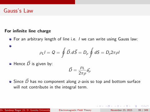
For infinite line charge
For an arbitrary length of line i.e. l we can write using Gauss law:
ρLl = Q =
∮~D.d ~S = Dρ
∮dS = Dρ2πρl
Hence ~D is given by:~D =
ρL2πρ
~aρ
Since ~D has no component along z-axis so top and bottom surfacewill not contribute in the integral term.
Dr. Sandeep Nagar (G. D. Goenka University) Electromagnetic Field Theory November 23, 2015 99 / 349

Gauss’s Law
For infinite sheet charge
Consider a sheet placed at z = 0 plane having uniform surface chargedensity of ρS (C .m−2)
As shown in figure:
Figure: Gaussian Surface about a Infinite Surface Charge
Dr. Sandeep Nagar (G. D. Goenka University) Electromagnetic Field Theory November 23, 2015 100 / 349

Gauss’s Law
For infinite sheet charge
We shall imagine Gaussian surface as a rectangle being cut by arectangular cross-section composed of charges from the sheet.
Since ~D is normal to the sheet ~D = Dz ~az .
Applying Guass’s law:
ρs
∫dS = Q =
∮~D.d ~S = DS [
∫top
dS +
∫bottom
dS ]
~D.d ~S = 0 for sides since ~D does not have any components along ~axand ~ay .
Dr. Sandeep Nagar (G. D. Goenka University) Electromagnetic Field Theory November 23, 2015 101 / 349

Gauss’s Law
For infinite sheet charge
If the area of top and bottom is A then one can write:
ρSA = Dz(A + A)
which implies:
~D =ρS2~az
which in turn implies that ~E is given by:
~E =~D
ε=ρS2ε~az
Dr. Sandeep Nagar (G. D. Goenka University) Electromagnetic Field Theory November 23, 2015 102 / 349

Gauss’s Law
For uniformly charged Sphere
Figure: Gaussian Surface about an uniformly charged sphere with two cases:r < a and r > a
Dr. Sandeep Nagar (G. D. Goenka University) Electromagnetic Field Theory November 23, 2015 103 / 349

Gauss’s Law
For uniformly charged Sphere
Dr. Sandeep Nagar (G. D. Goenka University) Electromagnetic Field Theory November 23, 2015 104 / 349

Gauss’s Law
For uniformly charged Sphere
Consider a uniformly charge sphere with radius a.
Two Gaussian surfaces can be considered with conditions
1 r < a2 r > a
~D is normal to surface of Gaussian surfaces and constant for a pointon them.
Enclosed charge for the case r < a is given by:
Qenc =
∫ρvdv = ρv
∫ 2π
φ=0
∫ 2π
θ=0
∫ r
r=0r2sin(θ)dr .dθ.dφ
which gives:
Qenc = ρv4
3πr2
Dr. Sandeep Nagar (G. D. Goenka University) Electromagnetic Field Theory November 23, 2015 105 / 349

Gauss’s law
Also,
Ψ =
∮~D.d ~S = Dr4πr2
Which gives
Dr4πr2 =4
3πa3ρv
Finally we get:
~D =a3
3r2ρv ~ar
for r ≥ a
Dr. Sandeep Nagar (G. D. Goenka University) Electromagnetic Field Theory November 23, 2015 106 / 349

Gauss’s law
~D =r
3ρv ~ar
for 0 < r ≤
~D =a3
3r2ρv ~ar
for r ≥ a
Dr. Sandeep Nagar (G. D. Goenka University) Electromagnetic Field Theory November 23, 2015 107 / 349

Gauss’s law
Figure: ~D variation with distance, with two cases: r < a and r > a
Dr. Sandeep Nagar (G. D. Goenka University) Electromagnetic Field Theory November 23, 2015 108 / 349

Electric potential
A quantity called potential (scalar) can be defined so that ~E can bedefined
Figure: Concept of electric potential derived using displacement of point charge Qin electric field ~EDr. Sandeep Nagar (G. D. Goenka University) Electromagnetic Field Theory November 23, 2015 109 / 349

Electric Potential
Work done (negative because work is done by external agent) in movingcharge Q from point A to point B:
W = −~F .d~l = −Q ~E .d~l
Hence total potential energy:
W = −Q∫ B
A
~E .d~l
A new quantity, potential energy per unit charge (unit = J/C = V ) canbe defined after which one can define potential difference VAB as
VAB =W
Q= −
∫ B
A
~E .d~l
Note: VAB is independent of path taken
Dr. Sandeep Nagar (G. D. Goenka University) Electromagnetic Field Theory November 23, 2015 110 / 349

Electric potential due to point charge
~E =Q
4πε0~ar
Now potential difference can be calculated as:
VAB = −∫ rB
rA
Q
4πε0~ar .dr ~ar
This results in:
VAB =Q
4πε0[
1
rA− 1
rB]
Which is same as:VAB = VA − VB
Where VA and VB are called absolute potentials at points A and Brespectively.VAB is potential at A w.r.t B
Dr. Sandeep Nagar (G. D. Goenka University) Electromagnetic Field Theory November 23, 2015 111 / 349

Electric potential
For point charges, its customary to take ∞ as the reference point,where potential is assumed to be zero (V∞ = 0).
If VA = 0 as rA → 0 then potential at any point rB → B will be givenby:
V =Q
4πε0r
In words: Potential at any point is the potential difference betweenthat point and a chosen point where potential is zero.
Potential at a distance r from the point charge is the work done perunit charge by an external agent in transferring a test charge frominfinity to that point
V = −∫ r
∞~E .d~l
Dr. Sandeep Nagar (G. D. Goenka University) Electromagnetic Field Theory November 23, 2015 112 / 349

Electric potential
If reference point is not considered to be infinity. then :
V =Q
4πε0r+ C
Where C is constant chosen as per reference point.
Dr. Sandeep Nagar (G. D. Goenka University) Electromagnetic Field Theory November 23, 2015 113 / 349

Electric potential
If the point charge Q is located at a position vector ~r ′ then:
V (~r) =Q
4πε0|~r − ~r ′ |Potential due to a point charge distribution:
V (~r) =1
4πε0
n∑k=1
Qk
|~r − ~r ′ |
Dr. Sandeep Nagar (G. D. Goenka University) Electromagnetic Field Theory November 23, 2015 114 / 349

Electric potential
Line charge distribution:
V (~r) =1
4πε0
∫L
ρL(~r ′)dl′
|~r − ~r ′ |
Surface charge distribution
V (~r) =1
4πε0
∫S
ρS(~r ′)dS′
|~r − ~r ′ |
Volume charge distribution
V (~r) =1
4πε0
∫v
ρv (~r ′)dv′
|~r − ~r ′ |
Dr. Sandeep Nagar (G. D. Goenka University) Electromagnetic Field Theory November 23, 2015 115 / 349

Relationship between ~E and V
Since potential is independent of path taken:
VBA = −VAB
This leads to the fact that
VAB + VBA = 0 =
∮~E .d~l
Physically, it will mean that net work done for moving a charge inclosed path will be zero.
Applying stokes theorem:∮~E .d~l =
∫(~∇× ~E ).d ~S = 0
~∇× ~E = 0
second Maxwell’s equation for electrostatics
Dr. Sandeep Nagar (G. D. Goenka University) Electromagnetic Field Theory November 23, 2015 116 / 349

Conservative nature of electric field
Figure: Conservative nature of electric field
Dr. Sandeep Nagar (G. D. Goenka University) Electromagnetic Field Theory November 23, 2015 117 / 349

Relationship between ~E and V
By definition of V :
V = −∫~E .d~l
Differential potential:
dV = −~E .d~l = −Exdx − Eydy − Ezdz
and
dV =∂V
∂xdx +
∂V
∂ydy +
∂V
∂zdz
Dr. Sandeep Nagar (G. D. Goenka University) Electromagnetic Field Theory November 23, 2015 118 / 349

Relationship between ~E and V
This leads to
Ex = −∂V∂x
and
Ey = −∂V∂y
and
Ez = −∂V∂z
Generalizing:
~E = −~∇VElectric field is gradient of a potential field.
Dr. Sandeep Nagar (G. D. Goenka University) Electromagnetic Field Theory November 23, 2015 119 / 349

Relationship between ~E and V
Negative sign shows that direction of ~E is opposite to direction ofincrease of V~E directs from lower to higher value of V .
Dr. Sandeep Nagar (G. D. Goenka University) Electromagnetic Field Theory November 23, 2015 120 / 349

Electric dipole
An electric dipole is composed of two charges of equal magnitude andseparated by a small distance.
Figure: DipoleDr. Sandeep Nagar (G. D. Goenka University) Electromagnetic Field Theory November 23, 2015 121 / 349

Electric dipole
V =Q
4πε0[
1
r1− 1
r2]
results in
V =Q
4πε0[r2 − r1r1r2
]
If r d then r2 − r1 ' d .cos(θ) and r1r2 = r2.
V =Q
4πε0[dcos(θ)
r2]
Now:d .cos(θ) = ~d .~ar
where~d = d ~az
Dr. Sandeep Nagar (G. D. Goenka University) Electromagnetic Field Theory November 23, 2015 122 / 349

Dipole moment
Dipole moment can be defined as:
~p = Q ~d
Hence potential can be defined in terms of dipole moment:
V =~p.~ar
4πε0r2
Now we assumed that ~p is directed from −Q to +Q.
If dipole center is not at the origin but at ~r ′ becomes:
V (~r) =~p.(~r − ~r ′)
4πε0|~r − ~r ′ |3
Dr. Sandeep Nagar (G. D. Goenka University) Electromagnetic Field Theory November 23, 2015 123 / 349

Dipole
A point charge is a monopole and it’s electric field varies inversely asr2 while its potential field varies inversely as r~E due to a dipole varies inversely as r3 while its potential variesinversely as r2
Dr. Sandeep Nagar (G. D. Goenka University) Electromagnetic Field Theory November 23, 2015 124 / 349

Electric flux lines
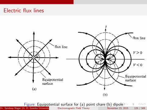
Electric flux line is an imaginary path or line drawn in such a way thatits direction at any point is the direction of the electric field at thatpoint.
Lines which are tangential at Electric field density ~D at every point.
Equipotential surface is a surface on which the potential is sameeverywhere.
Equipotential line is line generated by intersection of equipotentialsurfaces.
On an equipotential surface, work done will be zero becauseVA − VB = 0 i.e ∫
~E .d ~S = 0
Flux lines normal to equipotential surfaces/lines.
Dr. Sandeep Nagar (G. D. Goenka University) Electromagnetic Field Theory November 23, 2015 125 / 349
Electric flux lines
Figure: Equipotential surface for (a) point chare (b) dipoleDr. Sandeep Nagar (G. D. Goenka University) Electromagnetic Field Theory November 23, 2015 126 / 349

Energy Density in electrostatic fields
Energy present in a collection of charges can be estimated by energytaken for making up that collectionSuppose we wish to position three point charges Q1, Q2, Q3 in aninitially empty space as shown in figure.
Figure: Assembly of charges
Dr. Sandeep Nagar (G. D. Goenka University) Electromagnetic Field Theory November 23, 2015 127 / 349

Energy Density in electrostatic fields
Since initially, the space is empty so to move Q1 to position P1, nowork is required to transfer Q1 i.i.
W1 = 0
Work done in transferring Q2 from infinity to P2 :
W2 = Q2V21
Work done in transferring Q3 from infinity to P3 :
W3 = Q3V31 + Q3V32
Total work done for the systems of charges:
WE = W1 + W2 + W3 = 0 + Q2V21 + Q3(V31 + V32)
Dr. Sandeep Nagar (G. D. Goenka University) Electromagnetic Field Theory November 23, 2015 128 / 349

Energy Density in electrostatic fields
If the charges were placed in reverse order (on same positions)
WE = W3 + W2 + W 1
i.e.WE = 0 + Q2V23 + Q1(V12 + V13)
Adding both equations:
WE =1
2(Q1V1 + Q2V2 + Q3V3)
For n point charges, the associated energy (Joules) will be:
WE =1
2
n∑k=1
QkVk
Dr. Sandeep Nagar (G. D. Goenka University) Electromagnetic Field Theory November 23, 2015 129 / 349

Energy Density in electrostatic fields
For line charge distribution:
WE =1
2
∫ρLVdl
For surface charge distribution:
WE =1
2
∫ρSVdS
For volume charge distribution:
WE =1
2
∫ρvVdv
Dr. Sandeep Nagar (G. D. Goenka University) Electromagnetic Field Theory November 23, 2015 130 / 349

Energy Density in electrostatic fields
Sinceρv = ~∇. ~D
Hence
WE =1
2
∫(~∇. ~D)Vdv
Which results into:
WE =1
2
∫v
(~∇.v ~D)dv − 1
2( ~D.~∇V )dv
Divergence theorem states that:∫v
(~∇.v ~D)dv =
∮S
(V ~D).d ~S
Dr. Sandeep Nagar (G. D. Goenka University) Electromagnetic Field Theory November 23, 2015 131 / 349

Energy Density in electrostatic fields
Hence:
WE =1
2
∮S
(V ~D).d ~S − 1
2( ~D.~∇V )dv
For point charges V ∝ 1r and ~D ∝ 1
r2
For dipoles V ∝ 1r2 and ~D ∝ 1
r3
In the term 12
∮S(V ~D).d ~S the term V ~D must at-least vary as 1
r3 and
d ~S at-least vary as 1r2 which means as as surface becomes larger,
integral term tends to zero.
Since ~E = ~∇V and ~D = ε0E2
WE =1
2( ~D.~∇V )dv =
1
2
∫v
( ~D. ~E )dv =1
2
∫vε0E
2dv
Dr. Sandeep Nagar (G. D. Goenka University) Electromagnetic Field Theory November 23, 2015 132 / 349

Energy Density in electrostatic fields
WE =1
2( ~D.~∇V )dv =
1
2
∫v
( ~D. ~E )dv =1
2
∫vε0E
2dv
Hence the energy density can be defined as
wE =dW
dv=
1
2~D. ~E =
1
2ε0E
2 =D2
2ε0
Which gives the total electrostatic energy as:
WE =
∫vwEdv
Dr. Sandeep Nagar (G. D. Goenka University) Electromagnetic Field Theory November 23, 2015 133 / 349

Electric field in material space
Until now we have entertained issue where charges were placed in emptyspaceNow we shall consider the charges in material space.
Dr. Sandeep Nagar (G. D. Goenka University) Electromagnetic Field Theory November 23, 2015 134 / 349

Current and current density
Current through a given area is amount of charge passing throughthe area per unit time.
I =dQ
dt
Current density
~J =∆I
∆S
When current density vector is perpendicular to the surface areavector
∆I = Jn∆S
Dr. Sandeep Nagar (G. D. Goenka University) Electromagnetic Field Theory November 23, 2015 135 / 349

Current density
When ~J is not perpendicular to d ~S then
∆I = ~J.d ~S
Total current is given by:
I =
∫S
~J.d ~S
Three kinds of current densities:
1 convection current density (Does not involve conductors and does notfollow Ohm’s law)
2 conduction current density (Does involve conductors and follow Ohm’slaw)
3 displacement current density (Will be discussed later!)
Dr. Sandeep Nagar (G. D. Goenka University) Electromagnetic Field Theory November 23, 2015 136 / 349

Convection Current density
Consider a filament with flow of charge (charge density ρv ) at velocity~u
Figure: Current in filament
Dr. Sandeep Nagar (G. D. Goenka University) Electromagnetic Field Theory November 23, 2015 137 / 349

Convection Current density
Now:
∆I =∆Q
∆t= ρv∆S
∆l
∆t= ρv∆Suy
Current density in y direction:
Jy =∆I
∆S= ρvuy
In general~J = ρv ~u
Dr. Sandeep Nagar (G. D. Goenka University) Electromagnetic Field Theory November 23, 2015 138 / 349

Conduction current
When an electric field ~E is applied then a force ~F acts on charge, sayelectron, e which is given by:
~F = e ~E
Electron constantly collides with atoms arranged in the lattice.Suppose the average drift velocity is ~u and average time between twocollisions is τ .
As per Newton’s second law:
m~u
τ= −e ~E
Which implies:
~u = −eτ
m~E
Dr. Sandeep Nagar (G. D. Goenka University) Electromagnetic Field Theory November 23, 2015 139 / 349

Conduction current
For n electrons per unit volume:
ρv = −ne
Hence conduction current density can be given by:
~J = ρv ~u =ne2τ
m~E = σ ~E
This is expression for Ohm’s law in terms of conduction current.
Dr. Sandeep Nagar (G. D. Goenka University) Electromagnetic Field Theory November 23, 2015 140 / 349

Conductors in electric field
Electric behavior of conductors is given by expression for ~J
When an external electric field ~E is applied:
1 Positive charges move in the direction of the electric field ~F = +q ~E2 Negative charges move in the opposite direction of the electric field~F = −q ~E
These charges moves on the surface on opposite faces and makeinduced surface charge
This induced surface charge sets up an internal induced electric field~Ei
~Ei cancels Ee .
Dr. Sandeep Nagar (G. D. Goenka University) Electromagnetic Field Theory November 23, 2015 141 / 349

Conductors in electric field
A conductor is equipotential body i.e. ~E = −~∇V = 0
Now consider Ohm’s law: ~J = σ ~E
To maintain a finite current density ~J for a perfect conductor(σ →∞), ~Ei must vanish.
~E → 0⇔ σ →∞
If ~E = 0, according to Gauss law: ρv = 0 which implies Vab = 0
Dr. Sandeep Nagar (G. D. Goenka University) Electromagnetic Field Theory November 23, 2015 142 / 349

Conductors in electric field
When two ends of a conductor are maintained at a potentialdifference V , due to electromotive force, charges move and prevent aelectrostatic equilibrium.
An electric field must exist inside the conductor to sustain the flow ofcharges.~E 6= 0 inside the conductor.
The resistance provides the damping force to this movement ofcharges.
Dr. Sandeep Nagar (G. D. Goenka University) Electromagnetic Field Theory November 23, 2015 143 / 349

Conductors in electric field
Suppose the conductor is of length l and cross-section area S .
Electric field
E =V
l
Also the charge density is given as:
J =I
S
andJ = σE
Dr. Sandeep Nagar (G. D. Goenka University) Electromagnetic Field Theory November 23, 2015 144 / 349

Conductors in electric field
This gives:I
S= σE =
σV
l
Now we define resistance as:
R =V
I=
l
σS
We can define resistivity ρc = 1/σ which results in:
R =ρcS
Dr. Sandeep Nagar (G. D. Goenka University) Electromagnetic Field Theory November 23, 2015 145 / 349

Conductors in electric field
For conductors of non-uniform cross-section:
R =V
I=
~E .d~l
ρ~E .d ~S
Joule’s law defines the power in case of electrostatics as electrostaticforces times velocity: ∫
ρvdv ~E .~u =
∫~E .ρv ~udv
which gives
P =
∫~E . ~Jdv
Dr. Sandeep Nagar (G. D. Goenka University) Electromagnetic Field Theory November 23, 2015 146 / 349

Conductors in electric field
Power density:
wP =dP
dv= ~E . ~J = σ|~E |2
For a conductor of uniform cross-section dv = dSdl :
P =
∫LEdl
∫SJdS = VI = I 2R
Dr. Sandeep Nagar (G. D. Goenka University) Electromagnetic Field Theory November 23, 2015 147 / 349

Displacement current
When dielectrics are placed in an electric field, charges experienceforces but they are also bound strongly to nucleus.
Unlike conductors, where electrons can move within conductors,dielectric electrons can at-most displace themselves.
A dipole is formed where negative and positive charges are separatedby a distance.
This phenomenon is defined by polarization vector ~p:
~p = Q ~d
Dr. Sandeep Nagar (G. D. Goenka University) Electromagnetic Field Theory November 23, 2015 148 / 349

Atomic/Molecular Dipoles
Figure: Atomic/molecular dipoles
Dr. Sandeep Nagar (G. D. Goenka University) Electromagnetic Field Theory November 23, 2015 149 / 349

Displacement current
Since a dielectric have a number of atoms so combined effect of Ndipoles will be given by:
N∑k=1
Qk~dk
Intensity of polarization is given by dipole moment per unit volume:
~P =lim
∆v→0
∑Nk=1 Qk
~dk
∆v
Dr. Sandeep Nagar (G. D. Goenka University) Electromagnetic Field Theory November 23, 2015 150 / 349

Atomic/molecular dipoles
There are two kinds of dielectric materials:
1 Polar molecules are those which have permanent separations of charges
permanant dipole momentOn application of ~E , dipoles align to ~E
2 Non-polar molecules experience an induced dipole moment
non-permanant dipole momentOn application of ~E , dipole moment is created.
Dr. Sandeep Nagar (G. D. Goenka University) Electromagnetic Field Theory November 23, 2015 151 / 349

Dipoles moment
Figure: Dipole momentDr. Sandeep Nagar (G. D. Goenka University) Electromagnetic Field Theory November 23, 2015 152 / 349

Field due to Polarization
Consider a material with dipole moment per unit volume ( ~P )originating from dipole moments.
Potential due to this dipole moment:
dV =~P. ~aRdv
′
4πε0R2
Gradient in primed coordinates:
~∇′ =1
R=
~aRR2
This results in:
~P. ~aRR2
= ~P.~
∇′(1
R) = ~∇′ .
~P
R−
~∇′.~P
R
Dr. Sandeep Nagar (G. D. Goenka University) Electromagnetic Field Theory November 23, 2015 153 / 349

Field due to Polarization
substituting in expression for V :
V =
∫v ′
1
4πε0[ ~∇′ .
~P
R−
~∇′.~P
R]dv
′
Applying divergence to te first term:
V =
∫S ′
~P. ~a′n
4πε0RdS
′+
∫v ′
− ~∇′.~P
R]dv
′
Here ~a′n is outward unit normal to surface dS
′of the dielectric.
Two terms denotes potential due to surface and volume chargedistribution.ρps = ~P.~a and ρpv = −~∇.~P
Dr. Sandeep Nagar (G. D. Goenka University) Electromagnetic Field Theory November 23, 2015 154 / 349

Bound charges
ρps and ρpv are composed on bound charges which are different thanfree charges in a way such that, they are not free to move within adielectric; they are caused by displacement occurring due topolarization.
Total charges bound on surface:
Qb =
∮~P.d ~S =
∫ρpsdS
Total charge bound by this surface (within volume V ):
−Qb =
∫vρpvdv = −
∫v
~∇.~Pdv
Dr. Sandeep Nagar (G. D. Goenka University) Electromagnetic Field Theory November 23, 2015 155 / 349

Bound charges
Total charge = ∮ρPsdS +
∫vρPvdv = Qb − Qb = 0
This is logical because the dielectric was electrically neutral beforepolarization.
Dr. Sandeep Nagar (G. D. Goenka University) Electromagnetic Field Theory November 23, 2015 156 / 349

Dielectric with free charge
Lets consider the case where dielectric region contains free charge.
If ρv is free charge volume density and ρt is total volume chargedensity:
ρt = ρv + ρPv = ~∇.ε0~E
This implies:ρv = ~∇.ε0
~E − ρvThis results in:
ρv = ~∇.(ε0~E + ~P)
Dr. Sandeep Nagar (G. D. Goenka University) Electromagnetic Field Theory November 23, 2015 157 / 349

~D
We define a term~D = ε0
~E + ~P
which results in:ρv = ~∇. ~D
In words:Due to application of electric field ~E to dielectric material, fluxdensity is changed than it would have been in free space
Net effect of placing a dielectric inside an electric field ~E is to changethe electric field by the value ~P, to make it ~D
In this respect, free space can be defined a medium such that ~P = 0
Dr. Sandeep Nagar (G. D. Goenka University) Electromagnetic Field Theory November 23, 2015 158 / 349

Electric Susceptibility
We define:
~P = χeε0~E
Here χe is called the electric susceptibility because it determineshow much a material will polarize when an electric field will beapplied.
Dr. Sandeep Nagar (G. D. Goenka University) Electromagnetic Field Theory November 23, 2015 159 / 349

Dielectric constant
We know that~D = ε0
~E + ~P
and~P = χeε0
~E
hence~D = ε0(1 + χe)~E = ε0εr ~E
which can be written as~D = ε~E
whereε = ε0εr
andεr = 1 + χe =
ε
ε0
Dr. Sandeep Nagar (G. D. Goenka University) Electromagnetic Field Theory November 23, 2015 160 / 349

Dielectric constant
ε is permittivity of the dielectric
ε0 is permittivity of free space
εr is relative permittivity / dielectric constant
εr is a dimension-less quantity since
εr =ε
ε0
For free space εr = 1
For dielectric medium, εr > 1
Dr. Sandeep Nagar (G. D. Goenka University) Electromagnetic Field Theory November 23, 2015 161 / 349

Dielectric constant
So far we have discussed ideal dielectric material.
Practically, when ~E is sufficiently large, electrons are pulled out ofmolecules and bound charge becomes free charge. In this way, adielectric becomes a conductor. This phenomenon is called thedielectric breakdown.
Dielectric Strength is the maximum value of ~E which a dielectriccan tolerate without undergoing dielectric breakdown.
Dr. Sandeep Nagar (G. D. Goenka University) Electromagnetic Field Theory November 23, 2015 162 / 349

Types of dielectrics
Linear Dielectric: ~D varies linearly with ~E
Homogeneous: ε does not depend on coordinates.
Isotropic: ~D and ~E are in same direction.
Dr. Sandeep Nagar (G. D. Goenka University) Electromagnetic Field Theory November 23, 2015 163 / 349

Continuity equation
Since the total charge of the system must be conserved:
Iout = −dQin
dt=
∮~J.d ~S =
where Qin is the charge enclosed by the surface and Iout is currentcoming out of closed surface.
In words: Time rate of decrease of charge should be equal to netoutward flux
Using divergence theorem, one can write:∮~J.d ~S =
∫v
~∇. ~Jdv
Dr. Sandeep Nagar (G. D. Goenka University) Electromagnetic Field Theory November 23, 2015 164 / 349

Continuity equation
Also:
−dQin
dt= − d
dt
∫vρvdv = −
∫v
∂ρv∂t
dv
which implies: ∫v
~∇. ~Jdv = −∫v
∂ρv∂t
dv
This can be written as:
~∇. ~J = −∂ρv∂t
This is called continuity of current equation
Dr. Sandeep Nagar (G. D. Goenka University) Electromagnetic Field Theory November 23, 2015 165 / 349

Relaxation time
Ohm’s law:~J = σ ~E
Gauss’s law:
~∇. ~E =ρvε
Now:
~∇.σ ~E =σρvε
= −∂ρv∂t
which can be rearranged as a homogeneous linear differentialequation:
∂ρv∂t
+σ
ερv = 0
Dr. Sandeep Nagar (G. D. Goenka University) Electromagnetic Field Theory November 23, 2015 166 / 349

Relaxation time
Solving by separation of variables:
∂ρvρv
= −σε∂t
Upon integration:
ln(ρv ) = −σtε
+ ln(ρv0)
Hence the solution is:
ρv = ρv0 .e− t
Tr
whereTr =
ε
σ
and ρv0 is ρv at t = 0
Dr. Sandeep Nagar (G. D. Goenka University) Electromagnetic Field Theory November 23, 2015 167 / 349

Relaxation time
The solution of equation can be interpreted as follows:
When a charge is introduced at some interior point of a conductingmaterial, there is a decay of volume charge density as charge fromthat point moves towards the surface of the material.
Tr is called the relaxation/rearrangement time associated with thisprocess.
Technically, Tr is time it takes a charge placed in the interior of amaterial to drop to e−1 = 36.8 percent of initial value.
Its is small value for good conductors and large value for gooddielectric materials (insulators).
Dr. Sandeep Nagar (G. D. Goenka University) Electromagnetic Field Theory November 23, 2015 168 / 349

Boundary Conditions
So far we have considered homogeneous medium.
Inhomogeneous mediums are defined by boundaries.
Boundary conditions are conditions which a field must satisfy at theinterface/boundary of two dis-similar mediums.
Dr. Sandeep Nagar (G. D. Goenka University) Electromagnetic Field Theory November 23, 2015 169 / 349

Boundary Conditions
We start with Maxwell’s equations:∮~E .d~l = 0
and ∮~D.d ~S = Qenc
We also decompose the electric field in two orthogonal (perpendicularto each other) components:
~E = ~Et + ~En
Where Et represents the tangential component and ~En represents thenormal component.
Dr. Sandeep Nagar (G. D. Goenka University) Electromagnetic Field Theory November 23, 2015 170 / 349

Dielectric-Dielectric boundary condition
Figure: Dielectric-Dielectric boundary condition (a) defined in terms of ~E (b)
defined in terms of ~D
Dr. Sandeep Nagar (G. D. Goenka University) Electromagnetic Field Theory November 23, 2015 171 / 349

Dielectric-Dielectric boundary condition
Consider two different dielectrics differentiated by their permittivity:
ε1 = ε0εr1
and
ε2 = ε0εr2
Electric field can be decomposed into orthogonal components:
~E1 = ~E1t + ~E1n
and
~E2 = ~E2t + ~E2n
Dr. Sandeep Nagar (G. D. Goenka University) Electromagnetic Field Theory November 23, 2015 172 / 349

Dielectric-Dielectric boundary condition
Since ∮~E .d~l = 0
so
0 = E1t∆w − E1n∆h
2− E2n
∆h
2− E2t∆w + E2n
∆h
2+ E1n
∆h
2
Here Et = | ~Et | and En = | ~En|As ∆h→ 0, we get:
E1t = E2t
Tangential components of electric fields is same for both media i.e.tangential component of ~E is continuous across the boundary.
Dr. Sandeep Nagar (G. D. Goenka University) Electromagnetic Field Theory November 23, 2015 173 / 349

Dielectric-Dielectric boundary condition
What about ~D ?~D1 = ε1
~E1 and ~D2 = ε2~E2
Now
E1t = E2t ⇒~D1t
ε1=
~D2t
ε2
~D does changes across the interface, hence it is discontinuous.
Dr. Sandeep Nagar (G. D. Goenka University) Electromagnetic Field Theory November 23, 2015 174 / 349

Dielectric-Dielectric boundary condition
Consider the (b) figure, A Gaussian surface can be considered andapplying Gauss’s law:
~∇. ~E =ρvε
We can obtain(∆h→ 0):
∆Q = ρS∆S = D1n∆S − D2n∆S
This results inD1n − D2n = ρS
Where ρS is free charge density at interface.
If there is no free charge at interface (ρS = 0) then ~D is continuousat the interface.
Dr. Sandeep Nagar (G. D. Goenka University) Electromagnetic Field Theory November 23, 2015 175 / 349

Dielectric-Dielectric boundary condition
When we consider ~En instead of ~Dn we find that:
ε1E1n = ε2nE2n
~En is discontinuous.
These equations are called continuity equations for ~E and must befollowed by ~E for inhomogeneous media.
Dr. Sandeep Nagar (G. D. Goenka University) Electromagnetic Field Theory November 23, 2015 176 / 349

Refraction of ~E across the interface
Figure: Refraction of ~E across the interface
Dr. Sandeep Nagar (G. D. Goenka University) Electromagnetic Field Theory November 23, 2015 177 / 349

Refraction of ~E across the interface
E1sinθ1 = Et1 = E2t = E2sinθ2
and
D1cosθ1 = Dn1 = D2n = D2cosθ2
which can also be written as
ε1E1cosθ1 = Dn1 = D2n = ε2D2cosθ2
Which results in:
tanθ1
tanθ2=ε1
ε2
This is the law of refraction at a boundary which is devoid of free charge.
Dr. Sandeep Nagar (G. D. Goenka University) Electromagnetic Field Theory November 23, 2015 178 / 349

Conductor-dielectric boundary condition
Figure: Conductor-dielectric boundary condition
Dr. Sandeep Nagar (G. D. Goenka University) Electromagnetic Field Theory November 23, 2015 179 / 349

Conductor-dielectric boundary condition
We follow the same procedure and use the fact that ~E = 0 inside theconductor i.e for normal component E1n = 0
0 = 0∆w − 0∆h
2− E2n
∆h
2− E2t∆w + E2n
∆h
2+ 0
∆h
2
As ∆h→ 0 then
Et = 0
Similarly for the Gaussian surface, one can obtain:
∆Q = Dn.∆S − 0.∆S
which gives
Dn =∆Q
∆S= ρS
Dr. Sandeep Nagar (G. D. Goenka University) Electromagnetic Field Theory November 23, 2015 180 / 349

Conductor-Free Space boundary condition
Figure: Conductor - Free Space boundary condition
Dr. Sandeep Nagar (G. D. Goenka University) Electromagnetic Field Theory November 23, 2015 181 / 349

Free space is simply a special dielectric with εr = 1 so same boundaryconditions such as previous case exist i.e:
Dt = ε0Et = 0
and
Dn = ε0En = ρSDr. Sandeep Nagar (G. D. Goenka University) Electromagnetic Field Theory November 23, 2015 182 / 349

Electrostatic boundary value problem
Until now we have been dealing with situations where either chargedistribution and/or potential is known and we wish to find the ~E inentire region using Gauss law or the fact that ~E = −~∇.
These situations rarely exist for real life measurements.
Now we shall deal with issues where electrostatic conditions of chargeand/or potentials are defined at the interface and we wish to find the~E or V for entire region.
Such problems are called boundary value problems.
Dr. Sandeep Nagar (G. D. Goenka University) Electromagnetic Field Theory November 23, 2015 182 / 349

Poisson’s and Laplace’s equation
We know from Gauss’s law that
~∇. ~D = ~∇.ε ~E = ρv
since ~E = −~∇V so the equation can be rewritten as:
∇2V = −ρvε
In a free-charge free space, Poisson’s equation become Laplace’sequation i.e.
∇2V = 0
Dr. Sandeep Nagar (G. D. Goenka University) Electromagnetic Field Theory November 23, 2015 183 / 349

Uniqueness theorem
For particular boundary conditions, solutions of Poisson’s / Laplace’sequation is unique, regardless of method used. This is called theUniqueness Theorem.
Proof relies on the method of contradiction where we assume thatthere exist two solutions and then we show them to be same.
Dr. Sandeep Nagar (G. D. Goenka University) Electromagnetic Field Theory November 23, 2015 184 / 349

Proof of uniqueness theorem
Assuming that V1 and V2 are both solution to Laplace’s equation, then
∇2V1 = 0
and∇2V2 = 0
and lets assume that boundary condition is
V1 = V2
If we consider the difference in potential:
Vd = V2 − V2
this implies:
∇2Vd = 0
andVd = 0
Dr. Sandeep Nagar (G. D. Goenka University) Electromagnetic Field Theory November 23, 2015 185 / 349

Proof of uniqueness theorem
We now consider divergence theorem:∫v
~∇. ~A.dv =
∮S
~A.d ~S
Consider:~A = Vd
~∇Vd
Now we consider a vector identity
~∇. ~A = ~∇.(Vd~∇Vd) = Vd∇2Vd + ~∇Vd .~∇Vd = ~∇Vd .~∇Vd
Now: ∫v
~∇Vd .~∇Vd =
∮SVd~∇Vd .d ~S
RHS must vanish.
Dr. Sandeep Nagar (G. D. Goenka University) Electromagnetic Field Theory November 23, 2015 186 / 349

Proof of uniqueness theorem
∫v|~∇Vd |dv = 0
Since integration is always positive, hence:
~∇Vd = 0
This means that Vd is constant everywhere ⇒ Vd = V1 = V2
Dr. Sandeep Nagar (G. D. Goenka University) Electromagnetic Field Theory November 23, 2015 187 / 349

General Procedure for solving Laplace’s / Poisson’sequation
1 Solve Laplace’s / Poisson’s equation by1 Direct Integration when V is function of one variable2 Separation of variables when V is function of more than one variable.
Solution at this point is not unique by expressed in terms of unknownintegration constants.
2 Apply boundary conditions to determine the unique solution of V bygiving values to the unknown integration constants.
3 By applying ~∇V = ~E and D = ε~E calculate ~E and ~D4 Find Q using the fact
Q =
∫ρSdS
whereρS = Dn
where Dn is the normal component of ~D
Dr. Sandeep Nagar (G. D. Goenka University) Electromagnetic Field Theory November 23, 2015 188 / 349

Magnetostatics
SyllabusBiot-Savarts Law, Amperes circuit law, application of amperes law,magnetic flux density, magnetic scalar and vector potential, Magneticforces on a moving charge, magnetic materials, magnetic boundaryconditions.
Dr. Sandeep Nagar (G. D. Goenka University) Electromagnetic Field Theory November 23, 2015 189 / 349

Magnetostatistics
Magneto-statics is the study of static magnetic fields.
Dr. Sandeep Nagar (G. D. Goenka University) Electromagnetic Field Theory November 23, 2015 190 / 349

Biot-Savart law
dH ∝ I .dl .sinα
R2
The constant of proportionality is k whose value is 14π in SI units, which
makes Biot-savart law as:
dH =I .dl .sinα
4π.R2
Which can be written in vector form as:
d ~H =Id~l × ~aR
4πR2=
Id~l × ~R
4πR3
Figure: Direction of ~dHDr. Sandeep Nagar (G. D. Goenka University) Electromagnetic Field Theory November 23, 2015 191 / 349

Biot-Savart law
Figure: Biot-Savart Law
Dr. Sandeep Nagar (G. D. Goenka University) Electromagnetic Field Theory November 23, 2015 192 / 349

Biot-Savart law
Magnetic field intensity dH at a point P due to a differential currentcarrying element I .dl is proportional to I .dl and sine of angle betweencurrent carrying element and point P (i.e. sinα) and inverselyproportional to the square of the distance between P and element.
Dr. Sandeep Nagar (G. D. Goenka University) Electromagnetic Field Theory November 23, 2015 193 / 349

Magnetic field due to distributed current elements
For line current:
~H =
∫L
I ~dl × ~aR4πR2
For surface current:
~H =
∫S
~KdS × ~aR4πR2
For volume current:
~H =
∫v
~Jdv × ~aR4πR2
Here ~K and ~J are surface and volume current density
I ~dl ≡ ~KdS ≡ ~Jdv
Dr. Sandeep Nagar (G. D. Goenka University) Electromagnetic Field Theory November 23, 2015 194 / 349

Magnetic field due to distributed current elements
Figure: Current distributions: (a) Line current, (b) surface current, (c) volumecurrent
Dr. Sandeep Nagar (G. D. Goenka University) Electromagnetic Field Theory November 23, 2015 195 / 349

Magnetic field due to straigh filamentary conductor
Figure: Magnetic field due to straight filamentary conductor
Dr. Sandeep Nagar (G. D. Goenka University) Electromagnetic Field Theory November 23, 2015 196 / 349

Magnetic field due to straigh filamentary conductor
due to d~l , d ~H is given by:
d ~H =Id~l × ~R
4πR3
Now d~l = dz ~az and ~R = ρ~aρ − z ~az which leads to
d~l × ~R = ρdz ~aφ
Hence the total magnetic field intensity is given by:
~H =
∫Iρdz
4π[ρ2 + z2]3/2~aφ
Dr. Sandeep Nagar (G. D. Goenka University) Electromagnetic Field Theory November 23, 2015 197 / 349

Magnetic field due to straigh filamentary conductor
Now:
z = ρcotα
anddz = −ρcosec2αdα
This gives the total magnetic field intensity as:
~H =I
4πρ(cosα2 − cosα1) ~aφ
Dr. Sandeep Nagar (G. D. Goenka University) Electromagnetic Field Theory November 23, 2015 198 / 349

Magnetic field due to straigh filamentary conductor
Semi-finite conductor α1 = 900, α2 = 00 makes
~H =I
4πρ~aφ
infinite conductor: α1 = 1800, α2 = 00
~H =I
2πρ~aφ
Dr. Sandeep Nagar (G. D. Goenka University) Electromagnetic Field Theory November 23, 2015 199 / 349

Ampere’s circuit law
In words: Line integral of tangential component of ~H around a closedpath is same as net current enclosed by the path.∮
~H.d~l = Ienc
It is similar to Guass law
When current distribution is symmetrical, its is easy to find ~H.
Ampere law is a special case of Biot-Savart law.
Dr. Sandeep Nagar (G. D. Goenka University) Electromagnetic Field Theory November 23, 2015 200 / 349

Biot Savart law from Ampere Law
By applying stokes law, we get:
Ienc =
∮L
~H.d~l =
∫S
(~∇× ~H).d ~S =
∫S
~J.d ~S
This yields:
~∇× ~H = ~J
This is third maxwell’s equation.This essentially Ampere’s law in differential form.Since ~J 6= 0, hence magneto-static field is non-conservative field.
Dr. Sandeep Nagar (G. D. Goenka University) Electromagnetic Field Theory November 23, 2015 201 / 349

Infinite current length
Consider a long filamentary current I along z -axis.To analyze ~H at P, we imagine a closed path (Amperian path: pathon which Ampere law is followed) crossing P.For infinite current filament
~H =I
2πρ~aφ
Figure: ~H due to filamentary current
Dr. Sandeep Nagar (G. D. Goenka University) Electromagnetic Field Theory November 23, 2015 202 / 349

Infinite current length
If ρ is constant then ~H is constant i.e. magnetic field is same allaround the Amperian path.
This is analogous to Gaussian surface in electrostatics.
For closed path:
I =
∫Hφ ~aφ.ρdφ ~aφ = Hφ
∫ρdφ = Hφ.2πρ
which yields
~H =I
2πρ~aφ
As expected.
Dr. Sandeep Nagar (G. D. Goenka University) Electromagnetic Field Theory November 23, 2015 203 / 349

Infinite sheet of current
Figure: ~H due to infinite sheet of current
Dr. Sandeep Nagar (G. D. Goenka University) Electromagnetic Field Theory November 23, 2015 204 / 349

Infinite sheet of current
Consider a sheet in z = 0 plane having uniform current density~K = Ky ~ay .
As per Ampere law: ∮~H.d~l = Ienc = Kyb
For calculating ~H, we consider the infinite sheet to be composed of asmall filaments.
d ~H above or below the sheet due to a pair of filamentary (which isgiven by ~H = I
2πρ ~aφ)
As evident from the figure, resultant ~H has only x- componentbecause current travels in y -direction and current element is definedin z-direction.
Dr. Sandeep Nagar (G. D. Goenka University) Electromagnetic Field Theory November 23, 2015 205 / 349

Infinite sheet of current
~H on one side is sheet will be opposite in sign to the other side.
~H = H0 ~ax : z > 0~H = −H0 ~ax : z < 0
Also evaluating the line integral:∮~H.d~l = (
∫ 2
1+
∫ 3
2+
∫ 4
3+
∫ 1
4) ~H.d~l
which gives
= 0(−a) + (−H0)(−b) + 0(a) + H0(b)
Resulting finally as: ∮~H.d~l = 2H0b = kyb
Dr. Sandeep Nagar (G. D. Goenka University) Electromagnetic Field Theory November 23, 2015 206 / 349

title
i.e.
H0 =1
2Ky
This gives:
~H =1
2Ky ~ax : z > 0
~H = −1
2Ky ~ax : z < 0
In general:
~H =1
2~K × ~an
Where ~an is a unit normal vector directed from current sheet to the pointof interest.
Dr. Sandeep Nagar (G. D. Goenka University) Electromagnetic Field Theory November 23, 2015 207 / 349

Magnetic flux density
Just like ~D = ε0~E one can define
~B = µ0~H
Where µ0 is permeability of free space whose value is:
µ0 = 4π × 10−7
Units: Henry/mMagnetic flux through a surface:
Ψ =
∫S
~B.d ~S
Unit = WeberMagnetic flux density is found in W /m2 or Tesla.
Dr. Sandeep Nagar (G. D. Goenka University) Electromagnetic Field Theory November 23, 2015 208 / 349

Magnetic flux lines
Figure: Magnetic Flux Lines
Dr. Sandeep Nagar (G. D. Goenka University) Electromagnetic Field Theory November 23, 2015 209 / 349
Magnetic flux lines
Magnetic flux lines is the path to which ~B is tangential at every point inmagnetic field.It is the line along which magnetic needle of a compass will orient itself.Direction of ~B is taken as the north pointing direction.Magnetic field lines are closed and do not cross each other.
Dr. Sandeep Nagar (G. D. Goenka University) Electromagnetic Field Theory November 23, 2015 210 / 349

Magnetic flux lines
Figure: (a) Electric field lines need not be closed ⇒ electric monopoles exist (b)Magnetic field lines must be closed ⇒ magnetic monopoles do not exist
Dr. Sandeep Nagar (G. D. Goenka University) Electromagnetic Field Theory November 23, 2015 211 / 349

Gauss Law for magnetostatics
Since magnetic field lines are closed, hence∮~B.d ~S = 0
.
Although magneto-static field is not conserved, magnetic flux isconserved quantity.
Now ∮~B.d ~S =
∫v
~∇. ~Bdv = 0
which implies:
~∇. ~B = 0
This is Fourth Maxwell’s equation.
Dr. Sandeep Nagar (G. D. Goenka University) Electromagnetic Field Theory November 23, 2015 212 / 349

Maxwell’s equations
Differential form Integral form Remarks~∇. ~D = ρv
∮S~D.d ~S =
∫v ρvdv Gauss Law
~∇. ~B = 0∮S~B.d ~S = 0 No magnetic monopole
~∇× ~E = 0∮L~E .d~l = 0 Conservative ~E
~∇× ~H = ~J∮L~E .d~l =
∫S~J.d ~S Ampere Law
Dr. Sandeep Nagar (G. D. Goenka University) Electromagnetic Field Theory November 23, 2015 213 / 349

Magnetic Scalar and Vector Potentials
Just as electro static potential V is defined to be ~E = −~∇V we canwither define a scalar magnetic potential Vm or even a vectorpotential ~A.
When ~J = 0 then~H == ~∇Vm
Since ~J = ~∇× ~H we can write
~∇2Vm = 0
Since ~∇. ~B = 0 so we can define a vector potential ~A such that
~B = ~∇× ~A
Also:
Ψ =
∮L
~A.d~l
Dr. Sandeep Nagar (G. D. Goenka University) Electromagnetic Field Theory November 23, 2015 214 / 349

Force due to magnetic field
Force due to magnetic field can be considered for three cases:
1 Force on moving charged particle
2 Force on current element in an external ~B field
3 Force between two current elements
Dr. Sandeep Nagar (G. D. Goenka University) Electromagnetic Field Theory November 23, 2015 215 / 349

Magnetic force on moving charged particle
Electrostatic force on charge Q due to electric field ~E is given by:
~Fe = Q ~E
If charge Q moves with velocity ~u in magnetic field ~B the magneticforce is given by:
~Fm = Q~u × ~B
When both electric and magnetic fields are present:
~F = ~Fe + ~Fm = Q(~E + ~u × ~B)
~F is called Lorentz force.
Dr. Sandeep Nagar (G. D. Goenka University) Electromagnetic Field Theory November 23, 2015 216 / 349

Force on current element
We know that convection current is given by:
~J = ρv ~u
Now we also know:
Id~l = ~KdS = ~Jdv
So current element can be written as:
Id~l = ρv ~udv = dQ~u =dQ
dtd~l
Hence magnetic force:
d ~Fm = Id~l × ~B
Total magnetic force:~Fm =
∮L Id
~l × ~B
Dr. Sandeep Nagar (G. D. Goenka University) Electromagnetic Field Theory November 23, 2015 217 / 349

Force on current element
For line element:~Fm =
∮LId~l × ~B
For surface:
~Fm =
∮S
~kds × ~B
For volume:
~Fm =
∮v
~Jdv × ~B
Dr. Sandeep Nagar (G. D. Goenka University) Electromagnetic Field Theory November 23, 2015 218 / 349

Force between two current elements
Figure: Force two current element
Dr. Sandeep Nagar (G. D. Goenka University) Electromagnetic Field Theory November 23, 2015 219 / 349

Force between two current elements
Force d(d ~F1) on element I1d~l1 due to the field d ~B2:
d(d ~F1) = I1d~l1 × d ~B2
Biot-Savart law states that:
d ~B2 =µ0I2d~l2 × ~aR21
4πR221
This results in the force product to be:
d(d ~F1) =µ0I1d~l1 × (I2d~l2 × ~aR21)
4πR221
Total force:
~F1 =µ0I1I2
4π
∮L1
∮L2
d~l1 × (d~l2 × ~aR21)
R221
Dr. Sandeep Nagar (G. D. Goenka University) Electromagnetic Field Theory November 23, 2015 220 / 349

Magnetic Torque and Moment
If a current carrying loop is placed parallel to magnetic field, itexperiences a force that tends to rotate it.
Mathematically, this is given by torque.
Torque (Mechanical moment of force) is given by:
~T = ~r × ~F
Units: N.m
Dr. Sandeep Nagar (G. D. Goenka University) Electromagnetic Field Theory November 23, 2015 221 / 349

Magnetic Torque and Moment
Figure: Rectangular planar current carrying loop in uniform planar magnetic field
Dr. Sandeep Nagar (G. D. Goenka University) Electromagnetic Field Theory November 23, 2015 222 / 349

Magnetic Torque
Consider a rectangular loop of length l and width w placed in uniformmagnetic field ~B.
Since d~l ||~B along side 12 and 34 hence the force is exerted on thesesides is zero.
The total force:
~F = I
∫ 3
2d~l × ~B + I
∫ 1
4d~l × ~B
substituting values of length:
~F = I
∫ l
0dz~az × ~B + I
∫ 0
ldz~az × ~B
Dr. Sandeep Nagar (G. D. Goenka University) Electromagnetic Field Theory November 23, 2015 223 / 349

Magnetic Torque
If we assume ~F0 = IBl (Because ~B is uniform) then
~F = ~F0 − ~F0 = 0
Equal and opposite force acting on exactly opposite points producesno couple but when they act on different points on the loop, a coupleis created.
If normal to the plane of loop makes α with ~B:
| ~T | = |~F0|wsinα = BIlwsinα = BISsinα
where S = lw is cross-sectional area of loop.
Dr. Sandeep Nagar (G. D. Goenka University) Electromagnetic Field Theory November 23, 2015 224 / 349

Magnetic Torque
We define magnetic dipole moment:
~m = IS~an
Unit: A/m2
Its direction is normal to the loop.
Hence one can write the magnetic torque as:
~T = ~m × ~B
Dr. Sandeep Nagar (G. D. Goenka University) Electromagnetic Field Theory November 23, 2015 225 / 349

A Magnetic Dipole
A bar magnet or a small filamentary loop = magnetic dipole.Magnetic vector potential is defined as:
~A =µ0I
4π
∮d~l
r
Figure: Magnetic dipoleDr. Sandeep Nagar (G. D. Goenka University) Electromagnetic Field Theory November 23, 2015 226 / 349

A Magnetic Dipole
For r >> a , ~A has only φ dependence:
~A =µ0Iπa
2sinθ
4πr2~aφ
In terms of magnetic moment:
~A =µ0 ~m × ~ar
4πr2
Where ~m = Iπa2~az and ~az × ~ar = sinθ~aφ
Dr. Sandeep Nagar (G. D. Goenka University) Electromagnetic Field Theory November 23, 2015 227 / 349

A magnetic dipole
Now magnetic flux density is:
~B = ~∇× ~A
Which gives:
~B =µ0m
4πr2(2cosθ~ar − sinθ~aθ)
Figure: ~B due to current loop and bar magnetDr. Sandeep Nagar (G. D. Goenka University) Electromagnetic Field Theory November 23, 2015 228 / 349

A magnetic dipole
Assume an isolated magnetic charge signified by its pole strength anddepicted by Qm.
Suppose that the length of magnetic bar is l.
Dipole moment can be written as Qml
Torque can be defined as:
~T = ~m × ~B = Qm~l× ~B
Here~l points from South to North.
Force acting on magnetic charge:
~F = Qm~B
Dr. Sandeep Nagar (G. D. Goenka University) Electromagnetic Field Theory November 23, 2015 229 / 349

A magnetic dipole
A current carrying loop and bar magnet are equivalent magnetically,so
T = QmlB = ISB
which yields:
Qml = IS
Dr. Sandeep Nagar (G. D. Goenka University) Electromagnetic Field Theory November 23, 2015 230 / 349

Magnetization in materials
Similar to electric polarization, we can talk about magnetic polarization asper the nature of magnetic field.Atomic dipoles are made up by the unpaired valence electrons. Together,they make up the dipole moment of a magnetic material. Under theinfluence of an external magnetic field, this dipole moment experiencemagneto-static force, which characterizes the nature of magneticinteractions.
Dr. Sandeep Nagar (G. D. Goenka University) Electromagnetic Field Theory November 23, 2015 231 / 349

Magnetization
If there are N atoms in ∆v volume where kth atom has magneticmoment:
~M = lim∆v→0
∑Nk−1 ~mk
∆v
For differential volume d ~m = ~Mdv′.
Vector magnetic potential ~A due to d ~m is:
d ~A =µ0~M × ~aR
4πR2dv
′=µ0~M × ~R
4πR3dv
′
Now:
~R
R3= ~∇′ 1
R
Dr. Sandeep Nagar (G. D. Goenka University) Electromagnetic Field Theory November 23, 2015 232 / 349

Magnetization
So:
~A =µ0
4π
∫~M × ~∇′ 1
Rdv
′
Now:
~M × ~∇′ 1
R=
1
R~∇′ × ~M − ~∇′ ×
~M
R
Thus:
~A =µ0
4π
∫v ′
~∇′ × ~M
R− µ0
4π
∫v ′~∇′ ×
~M
R
Dr. Sandeep Nagar (G. D. Goenka University) Electromagnetic Field Theory November 23, 2015 233 / 349

Magnetization
As per vector identity:∫v ′~∇′ × ~F = −
∮ ′
S
~F × d ~S
Applying the vector identity to second integral:
~A =µ0
4π
∫v ′
~∇′ × ~M
Rdv
′+µ0
4π
∮S ′
~M × ~anR
dS′
We can write ~∇× ~M = ~J and ~M × ~an = ~K we can write:
~A =µ0
4π
∫v ′
~JbRdv
′+µ0
4π
∮S ′
~kbRdS
′
Dr. Sandeep Nagar (G. D. Goenka University) Electromagnetic Field Theory November 23, 2015 234 / 349

Magnetization
Hence we can define:
Bound volume current density:
~Jb = ~∇× ~M
Units: A/m2
Bound surface current density:
~Kb = ~M × ~anUnits: A/m~an is unit vector normal to the surface.
Dr. Sandeep Nagar (G. D. Goenka University) Electromagnetic Field Theory November 23, 2015 235 / 349

Magnetization
In free space ~M = 0:
~∇× ~H = ~Jf
which is same as
~∇×~B
µ0= ~Jf
In a material ~M 6= 0:
~∇×~B
µ0= ~Jf + Jb = ~J = ~∇× ~H + ~∇× ~M
which yields:
~B = µ0( ~H + ~M)
Dr. Sandeep Nagar (G. D. Goenka University) Electromagnetic Field Theory November 23, 2015 236 / 349

Linear magnetization
For linear materials: ~M depends linearly on ~H i.e.
~M = χm~H
where χm is dimensionless quantity called magnetic susceptibility
We can write:~B = µ0(1 + χm) ~H = µ ~H
or
~B = µ0µr ~H
whereµr = 1 + χm =
µ
µ0
Where µ is called the permeability (Henry.m)
Dr. Sandeep Nagar (G. D. Goenka University) Electromagnetic Field Theory November 23, 2015 237 / 349

Classification of magnetic materials
Figure: Classification of magnetic materials
Dr. Sandeep Nagar (G. D. Goenka University) Electromagnetic Field Theory November 23, 2015 238 / 349

Magnetic Boundary Conditions
Just as in electrostatics, we have to find boundary conditions for twodis-similar magnetic medias.
Figure: Magnetic boundary conditions
Dr. Sandeep Nagar (G. D. Goenka University) Electromagnetic Field Theory November 23, 2015 239 / 349

Magnetic Boundary Conditions
We shall use two laws of magneto-statics:∮~B.d ~S = 0
and ∮~H.d~l = I
We shall obtain:
~B1n = ~B2n
or
µ1~H1 = µ2
~H2
This essential means that normal component of ~B is continuouswhereas normal component of ~H isn’t.
Dr. Sandeep Nagar (G. D. Goenka University) Electromagnetic Field Theory November 23, 2015 240 / 349

Magnetic boundary conditions
Similarly, for closed path
K .∆w = H1t .∆w +H1n.∆h
2+H2n.
∆h
2−H2t .∆w−H2n.
∆h
2−H1n.
∆h
2
As ∆→ 0 we finally get
H1t − H2t = K
i.e.
B1t
µ1− B2t
µ2= K
Dr. Sandeep Nagar (G. D. Goenka University) Electromagnetic Field Theory November 23, 2015 241 / 349

Magnetic Boundary Condition
In general:
( ~H1 − ~H2)× ~an12 = ~K
Where ~an12 is the unit vector normal to interface and is directed frommedium 1 to 2.
For boundaries which are free of current i.e. ~K = 0
~H1t = ~H2t
or
B1t
µ1=
B2t
µ2
which essential signifies that tangential component of ~H is continuous.
Dr. Sandeep Nagar (G. D. Goenka University) Electromagnetic Field Theory November 23, 2015 242 / 349

Magnetic refraction
If the fields make and angle θ to the normal of interface:
B1cosθ1 = B1n = B2n = B2cosθ2
Also
B1
µ1sinθ1 = H1t = H2t =
B2
µ2sinθ2
Diving both we get:
tanθ1
tanθ2=µ1
µ2
Dr. Sandeep Nagar (G. D. Goenka University) Electromagnetic Field Theory November 23, 2015 243 / 349

Inductors and Inductances
A closed conducting loop carrying current I produces a magnetic field~B
This causes a flux Ψ to pass through such that:
Ψ =
∮~B.d ~S
This flux passes through each turn. Suppose there are N turns, thenone can define λ (flux linkage) as:
λ = NΨ
The the material surrounding the coiled conductor is linear then Ψ isproportional to current I producing it:
λ ∝ I ⇒ λ = LI
Dr. Sandeep Nagar (G. D. Goenka University) Electromagnetic Field Theory November 23, 2015 244 / 349

Inductors and Inductances
L is called Inductance of the circuit.
The circuit or part of circuit which have inductance is called aninductor.
Mathematically inductance can be defined as:
L =λ
I=
NΨ
I
Unit: Henry
Like capacitance, inductance gives an estimate about total magneticenergy stored in a material.
Wm =1
2LI 2
Dr. Sandeep Nagar (G. D. Goenka University) Electromagnetic Field Theory November 23, 2015 245 / 349

Inductor and Inductances
When two such circuits interact, we consider the term mutualinductance.
Figure: Mutual inductance of two current carrying coils
Dr. Sandeep Nagar (G. D. Goenka University) Electromagnetic Field Theory November 23, 2015 246 / 349

Inductor and Inductances
Four fluxes are involved here:
Ψ12 =
∫S1
~B2.d ~S
Hence mutual inductance M12 and M21 can be defined as:
M12 =λ12
I2=
N1Ψ12
I2and
M21 =λ21
I1=
N2Ψ21
I1
If the medium surrounding the coils is linear (absence of aferromagnetic material):
M12 = M21
Dr. Sandeep Nagar (G. D. Goenka University) Electromagnetic Field Theory November 23, 2015 247 / 349

Inductor and Inductances
Similarly self-inductances L1 and L2 can be defined as:
L1 =λ1
I1=
N1Ψ1
I1
and
L2 =λ2
I2=
N2Ψ2
I2
Total energy:
Wm =1
2L1I
21 +
1
2L2I
22 ±M12M21I1I2
Positive sign for last term is taken when currents in two circuits flowsuch that magnetic fields strengthen each other.
Dr. Sandeep Nagar (G. D. Goenka University) Electromagnetic Field Theory November 23, 2015 248 / 349

Magnetic Energy
Figure: Magnetic Energy
Dr. Sandeep Nagar (G. D. Goenka University) Electromagnetic Field Theory November 23, 2015 249 / 349

Magnetic Energy
Consider a differential volume dv .
Let the volume be covered with conducting sheets on top and bottomsurface with current ∆I
Inductance for this volume:
∆L =∆Ψ
∆I=µH∆x∆y
∆I
Also using ∆I = H∆y we can write:
∆Wm =1
2∆L∆I 2 =
1
2µH2∆x∆y∆z =
1
2µH2dv
Magneto-static energy density:
wm = lim∆→0
∆w
∆v=
1
2µH2 =
1
2B.H =
1
2µB2
Dr. Sandeep Nagar (G. D. Goenka University) Electromagnetic Field Theory November 23, 2015 250 / 349

Magnetostatic energy
Total magneto-static energy:
Wm =1
2
∫~B. ~H
Dr. Sandeep Nagar (G. D. Goenka University) Electromagnetic Field Theory November 23, 2015 251 / 349

Waves
Until now, we have considered time-invariant ~E (x , y , z) and ~H(x , y , z)
Now we shall consider dynamic/time-varying ~E (x , y , z , t) and~H(x , y , z , t)
Dr. Sandeep Nagar (G. D. Goenka University) Electromagnetic Field Theory November 23, 2015 252 / 349

Faraday law
Michael Faraday discovered in 1831 that static magnetic field do notproduce a current flow but time-varying magnetic fields produce aninduced voltage (electromotive force-emf ) in a closed circuit, which inturn causes the flow of current.
Faraday’s law:
Vemf = −dλ
dt= −N dΨ
dt
where N is number of turns and Ψ is magnetic flux through each turn.
Negative sign signifies that induced voltage acts to oppose the fluxproducing it. This is Lenz law which essentially signifies that directionof current flow in the circuit is such that induced magnetic fieldproduced by induced current will oppose the original magnetic field.
Dr. Sandeep Nagar (G. D. Goenka University) Electromagnetic Field Theory November 23, 2015 253 / 349

Faraday Law
Figure: Circuit showing emf-producing electric field ~Ef and electrostatic field ~Ee
~E = ~Ef + ~Ee
Where Electrostatic field: ~Ee = −~∇V and ~Ef = 0 outside the battery andhave opposite direction to ~Ee inside the battery.
Dr. Sandeep Nagar (G. D. Goenka University) Electromagnetic Field Theory November 23, 2015 254 / 349

Faraday Law
We know that:~E = ~Ef + ~Ee
For closed circuit, we would integrate of obtain:∮L
~E .d~l =
∮L
~Ef .d~l + 0 = −∫ N
P
~Ef .d~l
Through the battery.∮~E0.d~l = 0 because electrostatic field is conservative in nature.
~Ef is non-conservative.
Dr. Sandeep Nagar (G. D. Goenka University) Electromagnetic Field Theory November 23, 2015 255 / 349

Relationship between electric and magnetic fields
For a circuit of single turn (N = 1):
Vemf = −dΨ
dt=
∮L
~E .d~l = − d
dt
∫S
~B.d ~S
because
Ψ =
∫~B.d ~S
and Stoke’s theorem.
Here S is surface area of a circuit bounded by the closed path L.
Dr. Sandeep Nagar (G. D. Goenka University) Electromagnetic Field Theory November 23, 2015 256 / 349

Creating the variation of flux with time
A stationary loop in time varying magnetic field.
A time varying loop area in static magnetic field.
Time varying loop area in time varying magnetic field.
Dr. Sandeep Nagar (G. D. Goenka University) Electromagnetic Field Theory November 23, 2015 257 / 349

stationary loop in time varying magnetic field
Figure: stationary loop in time varying magnetic field
Dr. Sandeep Nagar (G. D. Goenka University) Electromagnetic Field Theory November 23, 2015 258 / 349

stationary loop in time varying magnetic field
Now:
Vemf =
∮L
~E .d~l = −∫S
∂ ~B
∂t.dS
EMF produced by time varying current (producing time varying ~B) ina stationary loop is called transformer emf.
Applying stokes law to the middle term:∫S
(~∇× ~E ).d ~S = −∫S
∂ ~B
∂t.dS
This implies:
(~∇× ~E ) = −∂~B
∂tThis is Maxwell’s equation for time varying magnetic field:
Dr. Sandeep Nagar (G. D. Goenka University) Electromagnetic Field Theory November 23, 2015 259 / 349

Moving loop in static ~B field
Figure: Moving loop in static ~B field
Dr. Sandeep Nagar (G. D. Goenka University) Electromagnetic Field Theory November 23, 2015 260 / 349

Moving loop in static ~B field
Magneto-static force on charge moving with uniform velocity ~u is:
~Fm = Q~u × ~B
We define the motional emf as:
~Em =~FmQ
= ~u × ~B
Hence:
Vemf =
∮L
~Em.d~l =
∮L(~u × ~B).d~l
Applying stokes theorem and equating integrands:
~∇× ~E = ~∇× (~u × ~B)
Dr. Sandeep Nagar (G. D. Goenka University) Electromagnetic Field Theory November 23, 2015 261 / 349

Moving loop in time varying ~B field
Combining transformer and motional emf:
Vemf =
∮L
~E .d~l = −∫S
∂ ~B
∂t.dS +
∫L(~u × ~B).d~l
which implies:
~∇× ~E = −∂~B
∂t+ ~∇× (~u × ~B)
Dr. Sandeep Nagar (G. D. Goenka University) Electromagnetic Field Theory November 23, 2015 262 / 349

Displacement current
For static EM field:~∇× ~H = ~J
Since divergence of a curl is zero, hence:
~∇.(~∇× ~H) = 0 = ~∇. ~J
But current continuity equation requires:
~∇. ~J = −∂ρv∂t6= 0
This equation of static fields needs modifications for time-varyingfields
Dr. Sandeep Nagar (G. D. Goenka University) Electromagnetic Field Theory November 23, 2015 263 / 349

Displacement current
We shall add a current density term:
~∇× ~H = ~J + ~Jd
Hence
~∇.(~∇× ~H) = 0 = ~∇. ~J + ~∇. ~JdSince current continuity equation demands:
~∇. ~J = −∂ρv∂t6= 0
Hence:
~∇. ~Jd = −~∇. ~J =∂ρv∂t
=∂
∂t(~∇. ~D) = ~∇.∂
~D
∂t
Dr. Sandeep Nagar (G. D. Goenka University) Electromagnetic Field Theory November 23, 2015 264 / 349

Displacement current
This implies that displacement current density ( ~Jd) can be definedapart from conduction current density ( ~J = σ ~E ) ,as:
~Jd =∂ ~D
∂t
which in turn implies that new maxwell’s equation for transient EMfields will be:
~∇× ~H = ~J +∂ ~D
∂t
Dr. Sandeep Nagar (G. D. Goenka University) Electromagnetic Field Theory November 23, 2015 265 / 349

Displacement current
Displacement current can be defined as:
Id =
∫~Jd .d ~S =
∫∂ ~D
∂t.d ~S
Dr. Sandeep Nagar (G. D. Goenka University) Electromagnetic Field Theory November 23, 2015 266 / 349

Time varying potential
For static EM waves, electric scalar potential:
V =
∫v
ρvdv
4πεR
and magnetic vector potential:
~A =
∫v
µJdv
4πεR
Now we would like to examine the potential under time varyingconditions
Dr. Sandeep Nagar (G. D. Goenka University) Electromagnetic Field Theory November 23, 2015 267 / 349

Time varying potential
~A was defined on the fact that ~∇. ~B = 0 which gives
~∇× ~A = ~B
This relation holds good for time varying magnetic fields too.
Now:
~∇× ~E = −d ~B
dt= −∂(~∇× ~A)
∂twhich implies that:
~∇× (~E +∂(~A)
∂t) = 0
The solution to which comes out to be:
~E +∂(~A)
∂t= −~∇V
Dr. Sandeep Nagar (G. D. Goenka University) Electromagnetic Field Theory November 23, 2015 268 / 349

Time varying potential
So if ~A and V are known then ~B and ~E can be found.
Now ~∇. ~D = ρv so:
~∇. ~E =ρvε
= −∇2V − ∂
∂t(~∇. ~A)
this implies
∇2V − ∂
∂t(~∇. ~A) =
ρvε
Dr. Sandeep Nagar (G. D. Goenka University) Electromagnetic Field Theory November 23, 2015 269 / 349

Time varying potential
We know that:
~B = ~∇× ~A
Taking curl on both sides and using the fact:
~∇× ~∇× ~A = µ ~J + εµ∂
∂t( ~∇V − ∂ ~A
∂t) = µ ~J − εµ~∇∂V
∂t− εµ∂
2 ~A
∂t2
According to a vector identity:
~∇× ~∇× ~A = ~∇(~∇. ~A)−∇2 ~A
Thus:
∇2 ~A− ~∇(~∇. ~A) = −µ ~J + εµ~∇∂V∂t
+ εµ∂2 ~A
∂t2
Dr. Sandeep Nagar (G. D. Goenka University) Electromagnetic Field Theory November 23, 2015 270 / 349

Time varying potential
To define a vector field uniquyely, its curl and divergence must bedefined. Now curl os ~A is already defined as
~∇× ~A = ~B
We shall choose to define the divergence of ~A as:
~∇. ~A = −µε∂V∂t
This will be termed as Lorentz condition for potential
Dr. Sandeep Nagar (G. D. Goenka University) Electromagnetic Field Theory November 23, 2015 271 / 349

Retarded potentials
By imposing Lorentz conditions, we get two wave equations:
∇2V − µε∂2V
∂t2= −ρv
ε
and
∇2 ~A− µε∂2 ~A
∂t2= −µ ~J
Potentials V and ~A are termed as retarded electric potential andretarded magnetic potential
Spped of propagation of wave is:
u =1√µε
In free space, u = c i.e speed of light
Dr. Sandeep Nagar (G. D. Goenka University) Electromagnetic Field Theory November 23, 2015 272 / 349

EM wave propagation
We shall now solve maxwell’s equations for following environments:
Free spaceσ = 0, ε = ε0, µ = µ0
Lossless dielectrics
σ = 0, ε = εr ε0, µ = µrµ0|σ << ωε
Lossy dielectricsσ 6= 0, ε = εr ε0, µ = µrµ0
Good conductors
σ ' ∞, ε = εr ε0, µ = µrµ0|σ >> ωε
where ω is angular frequency of the EM wave.
Dr. Sandeep Nagar (G. D. Goenka University) Electromagnetic Field Theory November 23, 2015 273 / 349

Wave theory: Basics
A general scalar wave equation in 1− D (z-direction) can be writtenas:
∂2E
∂t2− u2∂
2E
∂z2= 0
where u is wave-velocity.
Two solutions are:E+ = f (z − ut)
andE− = g(z + ut)
General solution can be written as linear superposition of solutions as:
E = f (z − ut) + g(z + ut)
Dr. Sandeep Nagar (G. D. Goenka University) Electromagnetic Field Theory November 23, 2015 274 / 349

Soltutions to wave equation
The functions f and g can have the forms like:
z ± ut
orsink(z ± ut)
orcosk(z ± ut)
ore jk(z±ut)
where k is a constant
Dr. Sandeep Nagar (G. D. Goenka University) Electromagnetic Field Theory November 23, 2015 275 / 349

Harmonic solutions
If we particularly assume the harmonic solutions (e jωt), the waveequation simplifies to:
d2Es
dz2+ β2Es = 0
where β = ω/u and Es is the phasor form of E .
solutions:E+ = Ae j(ωt−βz)
and
E− = Be j(ωt+βz)
and
E = Ae j(ωt−βz) + Be j(ωt+βz)
Dr. Sandeep Nagar (G. D. Goenka University) Electromagnetic Field Theory November 23, 2015 276 / 349

Understanding harmonic solutions
Consider the real part of E gives:
E = Asin(ωt − βz)
Properties:
A is amplitude of wave and has same units as E .(ωt − βz) is the phase (in radians) of wave.ω is angular frequency (radians/second)β is phase constant or wave number (radians/meter)
Dr. Sandeep Nagar (G. D. Goenka University) Electromagnetic Field Theory November 23, 2015 277 / 349

Harmonic solutions
Figure: Sine wave along with its characteristics propertiesDr. Sandeep Nagar (G. D. Goenka University) Electromagnetic Field Theory November 23, 2015 278 / 349

Wave properties
We can define wavelength (meters):
λ = uT
Frequency:
f =1
T
and
ω = 2πf =2π
λ
and
β =ω
u
group velocity:u = f λ
Dr. Sandeep Nagar (G. D. Goenka University) Electromagnetic Field Theory November 23, 2015 279 / 349

Wave propagation in lossy dielectrics
Most general case of wave propagation is that in lossy dielectric.Other cases can be derived from the same.
A lossy dielectric is a medium in which an EM wave loses power asit propagates due to poor conduction (σ 6= 0).
Consider such a lossy dielectric which is linear, homogeneous,isotropic and free of charge ρv = 0.
Dr. Sandeep Nagar (G. D. Goenka University) Electromagnetic Field Theory November 23, 2015 280 / 349

Wave propagation in lossy dielectrics
Maxwell’s equations:
~∇. ~Es = 0 (48)
~∇. ~Hs = 0 (49)
~∇× ~Es = −jωµ ~Hs (50)
~∇× ~Hs = (σ + jωε)~Es (51)
Dr. Sandeep Nagar (G. D. Goenka University) Electromagnetic Field Theory November 23, 2015 281 / 349

Wave propagation in lossy dielectrics
taking curl on both sides of third equation:
~∇× ~∇× ~Es = −jωµ~∇× ~Hs
Using vector identity:
~∇× ~∇× ~A = ~∇(~∇. ~A)−∇2 ~A
Since ~∇. ~E = 0 so
−~∇2 ~Es = −jωµ(σ + jωε)~Es
If we assume:γ2 = jωµ(σ + jωε)
where γ is termed as propagation constant.
Dr. Sandeep Nagar (G. D. Goenka University) Electromagnetic Field Theory November 23, 2015 282 / 349

Wave propagation in lossy dielectrics
Finally we get:~∇2 ~Es − γ2 ~Es = 0
By similar logic we can obtain:
~∇2 ~Hs − γ2 ~Hs = 0
These equations are called Helmholtz equations
Dr. Sandeep Nagar (G. D. Goenka University) Electromagnetic Field Theory November 23, 2015 283 / 349

Helmholtz equations
Since γ is a complex quantity:
γ = α + jβ
Hence- Re γ2 = β2 − α2 = ω2µε and|γ2| = β2 + α2 = ωµ
√σ2 + ω2ε2
Solving equations for α and β we get:
α = ω
√µε
2[
√1 + [
σ
ωε]− 1]
and
β = ω
√µε
2[
√1 + [
σ
ωε] + 1]
Dr. Sandeep Nagar (G. D. Goenka University) Electromagnetic Field Theory November 23, 2015 284 / 349

Electric field propagation
If we assume that wave propagates along ~az direction and ~Es has onlyx-component i.e.
~Exs(z)~ax
Substituting in~∇2 ~Es − γ2 ~Es = 0
we get:(~∇2 − γ2)~Exs = 0
which results in
[d2
dz2− γ2]Exs(z) = 0
because differential terms for x and y results in zero.
Dr. Sandeep Nagar (G. D. Goenka University) Electromagnetic Field Theory November 23, 2015 285 / 349

Electric field propagation
Hence finally we obtain
[d2
dz2− γ2]Exs(z) = 0
Its solution can be given as:
Exs(z) = E0e−γz + E
′0eγz
where E0 and E′0 are constants.
Field must be finite at infinity. This requires E′0 = 0
Inserting a time factor e jωt
~E (z , t) = Re[E0e−αze j(ωt−βz)~ax ]
Dr. Sandeep Nagar (G. D. Goenka University) Electromagnetic Field Theory November 23, 2015 286 / 349

Electric field propagation
This ultimately yields:
~E (z , t) = E0e−αzcos(ωt − βz)~ax
Figure: Propagation of |~E | in a lossy mediaDr. Sandeep Nagar (G. D. Goenka University) Electromagnetic Field Theory November 23, 2015 287 / 349

Magnetic field propagation
SImilar steps can be undertaken for propagation of magnetic field:
~H(z , t) = H0e−αzcos(ωt − βz) ~ay
where
H0 =E0
η
η is a complex quantity known as intrinsic impedance:
η =
√jωµ
σ + jωε= |η|e jθn
Dr. Sandeep Nagar (G. D. Goenka University) Electromagnetic Field Theory November 23, 2015 288 / 349

Magnetic field propagation
Also
|η| =
√µε
[1 + ( σωε)2]1/4
andtan2θn =
σ
ωε
where 0 ≤ θn ≤ 450
Using above equations, magnetic field can be written in terms ofcomponents of electric field:
~H(z , t) =E0
|η|e−αzcos(ωt − βz − θn)~ay
Dr. Sandeep Nagar (G. D. Goenka University) Electromagnetic Field Theory November 23, 2015 289 / 349

EM wave propagation
Now:~E (z , t) = E0e
−αzcos(ωt − βz)~ax
and~H(z , t) =
E0
|η|e−αzcos(ωt − βz − θn)~ay
α is called the attenuation constant for a medium (dB/m).
β is measure of phase shift per length i.e phase constant or wavenumber.
θn is phase difference between ~E an ~H.
Dr. Sandeep Nagar (G. D. Goenka University) Electromagnetic Field Theory November 23, 2015 290 / 349

Loss tangent
Loss tangent is derived from the ratio of ~Js and ~Jds :
| ~Js || ~Jds |
=|σ ~Es ||jωε~Es |
=σ
ωε= tanθ
tanθ is called loss tangent as it gives an idea about how lossy is amedium.
If loss tangent is small = good dielectric
If loss tangent is large = good conductor
Dr. Sandeep Nagar (G. D. Goenka University) Electromagnetic Field Theory November 23, 2015 291 / 349

Plane waves in lossless dielectrics
For lossless dielectrics:
σ = 0
ε = ε0εr
µ = µ0µr
which results in:
α = 0, β =√µε, u =
ω
β=
1√µε, λ =
2π
β
~E and ~H are in-phase.
Dr. Sandeep Nagar (G. D. Goenka University) Electromagnetic Field Theory November 23, 2015 292 / 349

Plane waves in free space
For free space
σ = 0
ε = ε0
µ = µ0
which results in:
α = 0, β = ω[√µ0ε0] =
ω
c, u =
1
[√µ0ε0]
= c , λ =2π
β
Also θn = 0, η = η0 where η0 is called intrinsic impedance of freespace
η0 =1
[√
1µ0ε0
]= 120π = 377Ω
Dr. Sandeep Nagar (G. D. Goenka University) Electromagnetic Field Theory November 23, 2015 293 / 349

Plane waves in free space
Electric field:~E = E0cos(ωt − βz)~ax
Magnetic field:
~H = H0cos(ωt − βz)~ay =E0
η0cos(ωt − βz)~ay
Direction of ~E , ~H and propagation direction:
~ak × ~aE = ~aH
and~ak × ~aH = −~aE
and~aE × ~aH = ~ak
Dr. Sandeep Nagar (G. D. Goenka University) Electromagnetic Field Theory November 23, 2015 294 / 349

Plane waves in free space
Figure: (a)Plot of ~E and ~H as function of z at t = 0, (b) Plot of ~E and ~H as seenfront front of propagation direction.
Dr. Sandeep Nagar (G. D. Goenka University) Electromagnetic Field Theory November 23, 2015 295 / 349

Plane wave in perfect conductor
For free space
σ ' ∞ε = ε0
µ = µ0µr
which results in:
α = β =
√ωµσ
2=
√πf µσ
u =ω
β=
√2ω
µσ
λ =2π
β
η =
√ωµ
σ]450
Dr. Sandeep Nagar (G. D. Goenka University) Electromagnetic Field Theory November 23, 2015 296 / 349

Plane wave in perfect conductor
~E leads ~H by 450
Electric field:~E = E0e
−αzcos(ωt − βz)~ax
Magnetic field:
~H =E0
[√
ωµσ ]
cos(ωt − βz − 450)~ay
Skin depth:As shown in above equations, ~E , ~H attenuates by a factor e−αz .The distance δ by which it attenuates by e−1 = 37% is called skindepth:
E0e−αδ = E0e
−1 ⇒ δ =1
α
Dr. Sandeep Nagar (G. D. Goenka University) Electromagnetic Field Theory November 23, 2015 297 / 349

Skin depth
Skin depth gives a measure to which an EM wave can penetrate amedium.
Figure: Skin depth
Dr. Sandeep Nagar (G. D. Goenka University) Electromagnetic Field Theory November 23, 2015 298 / 349

Poynting vector
Maxwell’s equation:
~∇× ~E = −µ∂~H
∂t
and
~∇× ~H = σ ~E + ε∂ ~E
∂t= ~J +
∂ ~D
∂t
Taking a dot product on both sides for second equation:
~E .(~∇× ~H) = ~E . ~J + ~E .∂ ~D
∂t
Now we know
~∇.(~E × ~H) = −~E .(~∇× ~H) + ~H.(~∇× ~E )
Dr. Sandeep Nagar (G. D. Goenka University) Electromagnetic Field Theory November 23, 2015 299 / 349

Poynting vector
~H.(~∇× ~E )− ~E .(~∇× ~H) = ~E . ~J + ~E .∂ ~D
∂t
Since
~∇× ~E = −µ∂~H
∂tso
− ~H.∂~B
∂t− ~E .(~∇× ~H) = ~E . ~J + ~E .
∂ ~D
∂t
which can be written as:
−~E .(~∇× ~H) = ~E . ~J + ε~E .∂ ~E
∂t+ µ ~H.
∂ ~H
∂t
Dr. Sandeep Nagar (G. D. Goenka University) Electromagnetic Field Theory November 23, 2015 300 / 349

Poynting vector
Two time derivatives can be rearranged as:
ε~E .∂ ~E
∂t=
∂
∂t(
1
2~D. ~E )
and
µ ~H.∂ ~H
∂t=
∂
∂t(
1
2~B. ~H)
which ultimately gives
−~E .(~∇× ~H) = ~E . ~J +∂
∂t(
1
2~D. ~E ) +
∂
∂t(
1
2~B. ~H)
Dr. Sandeep Nagar (G. D. Goenka University) Electromagnetic Field Theory November 23, 2015 301 / 349

Poynting vector
Integrating over the volume
−∫v
~E .(~∇× ~H) =
∫v
~E . ~J +
∫v
∂
∂t(
1
2~D. ~E ) +
∫v
∂
∂t(
1
2~B. ~H)
Applying divergence theorem to right hand side:∮s(~E × ~H).d ~S =
∫v
~E . ~J +
∫v
∂
∂t(
1
2~D. ~E ) +
∫v
∂
∂t(
1
2~B. ~H)
Dr. Sandeep Nagar (G. D. Goenka University) Electromagnetic Field Theory November 23, 2015 302 / 349

Poynting vector
Finally: ∮S
(~E × ~H).d ~S =
∫vσE 2 +
∂
∂t
∫v
[ε∂E 2
2+ µ
∂H2
2]
LHS is total power leaving the volume
First term on RHS is rate of decrease in energy stored in electric andmagnetic fields
Ohmic power dissipated
The equation is known as Poynting theorem and ~E × ~H is called thePoynting vector
Dr. Sandeep Nagar (G. D. Goenka University) Electromagnetic Field Theory November 23, 2015 303 / 349

Reflection of a plane wave at normal incidence
Consider the case as below:
Figure: Reflection of a plane wave at normal incidence
Dr. Sandeep Nagar (G. D. Goenka University) Electromagnetic Field Theory November 23, 2015 304 / 349

Reflection of a plane wave at normal incidence
Incident wave: ~Ei , ~Hi is traveling in +~az in medium 1 where wesuppress the time factor e jωt :
~Eis(z) = Eioe−γ1z~ax
and~His(z) = Hioe
−γ1z~ay =Ei0
η1e−γ1z~ay
Reflected wave: ~Er , ~Hr is traveling in −~az in medium 1 where wesuppress the time factor e jωt :
~Ers(z) = Eroe−γ1z~ax
and~Hrs(z) = Hroe
−γ1z(−~ay ) = −Ero
η1e−γ1z~ay
Dr. Sandeep Nagar (G. D. Goenka University) Electromagnetic Field Theory November 23, 2015 305 / 349

Reflection of a plane wave at normal incidence
Transmitted wave: ~Et , ~Ht is traveling in +~az in medium 2 where wesuppress the time factor e jωt :
~Ets(z) = Etoe−γ2z~ax
and~Hts(z) = Htoe
−γ2z(~ay ) = −Eto
η2e−γ2z~ay
Dr. Sandeep Nagar (G. D. Goenka University) Electromagnetic Field Theory November 23, 2015 306 / 349

Reflection of a plane wave at normal incidence
Medium 1 has incident and reflected wave whereas medium 2 hastransmitted wave.
~E1 = ~Ei + ~Er
and~H1 = ~Hi + ~Hr
Medium 2 only contain reflected wave:
~E2 = ~Et
and~H2 = ~Ht
Dr. Sandeep Nagar (G. D. Goenka University) Electromagnetic Field Theory November 23, 2015 307 / 349

Reflection of a plane wave at normal incidence
At z = 0 boundary conditions dictate that tangential components of~E , ~H are continuous.
At z = 0:
~E1tan = ~E2tan ⇒ ~Ei (0) + ~Er (0) = ~Et(0)⇒ Eio + Ero = Eto
and
~H1tan = ~H2tan ⇒ ~Hi (0) + ~Hr (0) = ~Ht(0)⇒ 1
η1(Eio + Ero) =
1
η2Eto
This yields:
Ero =η2 − η1
η2 + η1Eio ,Eto =
2η2
η2 + η1Eio
Dr. Sandeep Nagar (G. D. Goenka University) Electromagnetic Field Theory November 23, 2015 308 / 349

Reflection and Transmission coefficients
Reflection coefficient:
Γ =Ero
Eio=η2 − η1
η2 + η1
Transmission coefficient:
τ =Eto
Eio=
2η2
η2 + η1
Relationship:τ = 1 + Γ
Both Γ and τ are dimensionless
o ≤ |Γ| ≤ 1
Dr. Sandeep Nagar (G. D. Goenka University) Electromagnetic Field Theory November 23, 2015 309 / 349

Special case
Suppose medium 1 is perfect dielectric (σ1 = 0) and medium 2 isperfect conductor (σ2 ' ∞).
In this case: η2 = 0: Γ = −1 and τ = 0 meaning that wave is totallyreflected.
This is expected because electric field inside conductor should vanishmeaning there is no transmitted wave.
When totally reflected wave mixes with incident wave to make astanding wave consisting of two traveling waves ~Ei , ~Er making astationary pattern because both travel with equal amplitude but inopposite directions.
Dr. Sandeep Nagar (G. D. Goenka University) Electromagnetic Field Theory November 23, 2015 310 / 349

Standing waves
Standing wave in medium 1:
~E1s = ~Eis + ~Ers = (Eioe−γ1z + Eroe
−γ1z)
But
Γ =Ero
Eio= −1, σ1 = 0, α1 = 0, γ1 = jβ1
Hence:
~E1s = −Eio(e jβ1z − e−jβ1z)~ax = −2jEiosinβiz~ax
which means that
~E1 = Re(~E1sejωt) = 2Eiosinβ1zsinωt~ax
Dr. Sandeep Nagar (G. D. Goenka University) Electromagnetic Field Theory November 23, 2015 311 / 349

Standing waves
We obtained:~E1 = 2Eiosinβ1zsinωt~ax
By similar procedure we can obtain:
~H1 =2Eio
η1cosβ1zcosωt~ay
Figure: Standing waveDr. Sandeep Nagar (G. D. Goenka University) Electromagnetic Field Theory November 23, 2015 312 / 349

Standing wave ratio
Standing wave ratio s can be defined as:
s =|~E1|max
|~E1|min
=| ~H1|max
| ~H1|min
=1 + Γ
1− Γ
Also:
|Γ| =s − 1
s + 1
Since |Γ| ≤ 1 hence 1 ≤ s ≤ ∞SWR is a dimensionless quantity
SWR can also be expressed in dB as:s(dB) = 20log10s
Dr. Sandeep Nagar (G. D. Goenka University) Electromagnetic Field Theory November 23, 2015 313 / 349

Transmission Lines Introduction
Until now we discussed infinite space for the medium
Now we shall discuss guiding mediums of finite dimensions and studypropagation of EMW.
These guiding mediums are called transmission lines
They are essentially made up of two or more parallel conductors usedto connect source and load
Source is the EM power generator (oscillator, hydroelectric generator,transmitter)
Load is EM reception station (antenna, oscilloscope etc.)
Dr. Sandeep Nagar (G. D. Goenka University) Electromagnetic Field Theory November 23, 2015 314 / 349

Transmission line parameters
1 R = resistance per unit length
2 G = conductance per unit length
3 C = capacitance per unit length
4 L = inductance per unit length
Dr. Sandeep Nagar (G. D. Goenka University) Electromagnetic Field Theory November 23, 2015 315 / 349

Transmission line parameters
Transmission line parameters are uniformly distributed over thetransmission line.
Figure: Distribution of line parameters over a transmission line
Dr. Sandeep Nagar (G. D. Goenka University) Electromagnetic Field Theory November 23, 2015 316 / 349

Transmission line parameters
For each line, conductors are characterized by σc , µc , εc = ε0 andhomogeneous dielectric separating the conductors is characterized byσ, µ, ε.
G 6= 1/R because R shows the AC resistance per unit length ofconductor and G is the conductance per unit length due to dielectricmedium separating the conductors.
L is the external inductance per unit length since effects of internalinductance is negligible at high frequency.
For all transmission lines:LC = µε
and
G
C=σ
ε
Dr. Sandeep Nagar (G. D. Goenka University) Electromagnetic Field Theory November 23, 2015 317 / 349

Coaxial cable
Figure: Coaxial line connecting a generator and load (b) ~E , ~H fields in coaxial line
Dr. Sandeep Nagar (G. D. Goenka University) Electromagnetic Field Theory November 23, 2015 318 / 349

Coaxial cable
When switch S is closed:
Inner conductor is made positive w.r.t outer one~E will point radially outward from inner conductor to outer conductingsheath.Ampere law states that ~H field encircles the current carrying conductor.Poynting vector ~E × ~H points along the transmission line.
Dr. Sandeep Nagar (G. D. Goenka University) Electromagnetic Field Theory November 23, 2015 319 / 349

Transmission line equations
Transmission line equations are also called as telegrapher’sequations since telegraph was first direct application of transmissionline based EMW communication system.
Figure: L-type equivalent circuit model of a differential length ∆z for atwo-conductor transmission line
Dr. Sandeep Nagar (G. D. Goenka University) Electromagnetic Field Theory November 23, 2015 320 / 349

Transmission line equations
The model is called the L-type equivalent circuit.
Here we assume that the wave propagates along the +z-direction(from generator to load).
By applying Kirchoff’s voltage law to outer loop:
V (z , t) = R∆zI (z , t) + L∆z∂I (z , t)
∂t+ V (z + z∆z , t)
which can also be simply written as
V (z + z∆z , t)− V (z , t)
∆z= RI (z , t) + L
∂I (z , t)
∂t
Dr. Sandeep Nagar (G. D. Goenka University) Electromagnetic Field Theory November 23, 2015 321 / 349

Transmission line equations
Taking limits:
lim∆z→0
(V (z + z∆z , t)− V (z , t)
∆z) = RI (z , t) + L
∂I (z , t)
∂t
Hence
−∂V (z , t)
∂t= RI (z , t) + L
∂I (z , t)
∂t
Dr. Sandeep Nagar (G. D. Goenka University) Electromagnetic Field Theory November 23, 2015 322 / 349

Transmission line equation
Similarly, applying Kirchoff’s current law to the main node of thecircuit:
I (z , t) = I (z+∆z , t)+∆I = I (z+∆z , t)+G∆zV (z+∆z , t)+C∆z∂V (z + ∆z , t)
∂t
We shall ultimately get:
−∂I (z , t)
∂t= GV (z , t) + C
∂V (z , t)
∂t
Dr. Sandeep Nagar (G. D. Goenka University) Electromagnetic Field Theory November 23, 2015 323 / 349

Transmission line equations
We obtained two differential equations:
−∂V (z , t)
∂t= RI (z , t) + L
∂I (z , t)
∂t
and
−∂I (z , t)
∂t= GV (z , t) + C
∂V (z , t)
∂t
Dr. Sandeep Nagar (G. D. Goenka University) Electromagnetic Field Theory November 23, 2015 324 / 349

Tranmission line equations
If we assume harmonic time dependence:
V (z , t) = Re[Vsejωt ]
andI (z , t) = Re[Ise
jωt ]
Hence our differential equations simplifies as:
−dVs
dz= (R + jωL)Is
and
−dIsdz
= (G + jωC )Vs
These are coupled differential equations where Vs and Is are coupled.
Dr. Sandeep Nagar (G. D. Goenka University) Electromagnetic Field Theory November 23, 2015 325 / 349

Transmission line equations
Taking the second derivative:
d2Vs
dz2= (R + jωL)(G + jωC )Vs
which yields:d2Vs
dz2− γ2Vs = 0
Similarly:d2Isdz2− γ2Is = 0
Hereγ = α + jβ =
√(R + jωL)(G + jωC )
Dr. Sandeep Nagar (G. D. Goenka University) Electromagnetic Field Theory November 23, 2015 326 / 349

Transmission line parameters
These are similar to wave equations we have already studied
γ is propagation constant
α is attenuation constant
β is phase constant
Wavelength and wavenumber can be written as:
λ =2π
β
andu =
ω
β= f λ
Dr. Sandeep Nagar (G. D. Goenka University) Electromagnetic Field Theory November 23, 2015 327 / 349

Transmission line parameters
Solutions:Vs = V+
o e−γz + V−o e−γz
andIs = I+
o e−γz + I−o e−γz
Here V+o ,V
−o , I
+o , I
−o are wave amplitudes
The + and − sign depicts the wave traveling in +z and −z directions.
We also obtain:
V (z , t) = Re[Vs(z)e jωt ] = V+o e−αzcos(ωt−βz)+V−o e−αzcos(ωt−βz)
Dr. Sandeep Nagar (G. D. Goenka University) Electromagnetic Field Theory November 23, 2015 328 / 349

Transmission Line parameters
Characteristic impedance
Zo =V+o
I+o
= −V−oI−o
=R + jωL
γ=
γ
G + jωC
which can be simplified to:
Zo =
√R + jωL
G + jωC= Ro + jXo
Dr. Sandeep Nagar (G. D. Goenka University) Electromagnetic Field Theory November 23, 2015 329 / 349

Lossless line
R = G = 0
Conductor is perfect σc ' ∞ and dielectric is lossless σ = 0.
α = 0
γ = jβ = jω√LC
u =ω
β=
1√LC
= f λ
Xo = 0
Zo = Ro =
√L
C
Dr. Sandeep Nagar (G. D. Goenka University) Electromagnetic Field Theory November 23, 2015 330 / 349

Distortionless line
A signal is usually composed of a number of frequencies having thierspecific amplitudes.
If attenuation is frequency dependent then signal is distorted.
When α is frequency independent and phase constant β linearlydepends on frequency, transmission line is termed distortion-less.
Such a line has:
R
L=
G
C
Dr. Sandeep Nagar (G. D. Goenka University) Electromagnetic Field Theory November 23, 2015 331 / 349

Distortionless line
Propagation constant:
γ =
√RG (1 +
jωL
R)(1 +
jωC
G)
which results in
γ =√RG (1 +
jωL
R) = α + jβ
whereα =√RG , β = ω
√LC
Note that here α is independent of ω or f
β linearly depends on ω or f .
Dr. Sandeep Nagar (G. D. Goenka University) Electromagnetic Field Theory November 23, 2015 332 / 349

Distortionless line
Zo =
√R(1 + jωL/R)
G (1 + jωC/G )=
√R
G=
√L
C= Ro + jXo
which gives
Ro =
√R
G=
√L
C
andXo = 0
and
u =ω
β=
1√LC
= f λ
Dr. Sandeep Nagar (G. D. Goenka University) Electromagnetic Field Theory November 23, 2015 333 / 349

Input Impedance
consider a transmission line of length ` characterized by γ,Zo
connected to a load ZL.
Figure: (a) Input impedance of a line terminated by a load (b) equivalent circuitDr. Sandeep Nagar (G. D. Goenka University) Electromagnetic Field Theory November 23, 2015 334 / 349

Input impedance
Let the transmission line has generator at z = 0 and load at z = `.
Vs = V+o e−γz + V−o e−γz
and
Is =V+o
Zoe−γz − V−o
Zoe−γz
These wave equations explain the behavior of voltage and current.To find V+
o ,V−o , terminal conditions must be given say
Vo = V (z = 0), Io = I (z = 0)
Substituting them we get
V+o =
1
2(Vo + Zo Io)
and
V−o =1
2(Vo − Zo Io)
Dr. Sandeep Nagar (G. D. Goenka University) Electromagnetic Field Theory November 23, 2015 335 / 349

Input impedance
If input impedance is Zin, then the input voltage Vo and Io :
Vo =Zin
Zin + ZgVg , Io =
Vg
Vin + Vg
On the other hand, if we are given conditions at load end:
VL = V (z = `), IL = I (z = `)
we get:
V+o =
1
2(VL + Zo IL)eγ`
and
V−o =1
2(VL − Zo IL)e−γ`
Dr. Sandeep Nagar (G. D. Goenka University) Electromagnetic Field Theory November 23, 2015 336 / 349

Input impedance
When input impedance Zin = Vs(z)Is(z) is given at any point on the
transmission line:
Zin =Vs(z)
Is(z)=
Zo(V+o ) + V−o
V+o )− V−o
Utilizing the fact that:
coshγ` =eγ` + e−γ`
2, sinhγ` =
eγ` − e−γ`
2, tanhγ` =
eγ` − e−γ`
eγ` + e−γ`
This yields:
Zin = Zo [ZL + Zotanhγ`
Zo + ZLtanhγ`]
This expression stands true for Lossy transmission line.
Dr. Sandeep Nagar (G. D. Goenka University) Electromagnetic Field Theory November 23, 2015 337 / 349

Input impedance
For lossless line γ = jβ which leads to tanhjβ` = jtanβ`
Hence the expression for input impedance:
Zin = Zo [ZL + jZotanβ`
Zo + jZLtanβ`]
The equation essentially means that input impedance variesperiodically along the length of line
β` is called electrical length of the line (expressed indegree/radians).
Dr. Sandeep Nagar (G. D. Goenka University) Electromagnetic Field Theory November 23, 2015 338 / 349

Standing wave ratio
We can define Voltage reflection coefficient at load:
ΓL =V−o eγ`
V+o e−γ`
=ZL − Zo
ZL + Zo
Standing wave ratio:
s =Vmax
Vmin=
Imax
Imin=
1 + |ΓL|1− |ΓL|
Imax = Vmax/Zo and Imin = Vmin/Zo
Relationship of input impedance and standing wave ratio
Zin|max =Vmax
Imin= sZo ,Zin|min =
Vmin
Imax=
Zo
s
Dr. Sandeep Nagar (G. D. Goenka University) Electromagnetic Field Theory November 23, 2015 339 / 349

Average power
Average power:
Pav =1
2Re[Vs(`)I ∗s (`)] =
|V+0 |2
2Zo(1− |Γ|2)
Factor of 1/2 comes into play since we are dealing with peak values,instead of r.m.s values.
First term refers to input power and second term refers to reflectedpower.
Maximum power is delivered to load when Γ = 0 i.e. due toimpedance matching, there isn’t any reflected wave.
Dr. Sandeep Nagar (G. D. Goenka University) Electromagnetic Field Theory November 23, 2015 340 / 349

Smith Chart
Smith chart is a graphical means of calculating transmission lineparameters.
Graphical indication of impedance of a transmission line as one movesalong the line.
Dr. Sandeep Nagar (G. D. Goenka University) Electromagnetic Field Theory November 23, 2015 341 / 349

Procedure to make a smith chart
1 Construct a unit circle (radius = |Γ| ≤ 1)
2 We shall use the relations:
Γ =ZL − Zo
ZL + Zo
and
Γ∠θL = Γi + jΓr
where Γi and Γr are real and imaginary parts of reflection coefficientΓ.
3 Calculating normalized impedance
zL =ZL
Zo= r + jx
Dr. Sandeep Nagar (G. D. Goenka University) Electromagnetic Field Theory November 23, 2015 342 / 349

Procedure to make a smith chart
Γ can be written as:
Γ = Γr + jΓi =zL − 1
zL + 1
which results in:
r =1− Γ2
r − Γ2i
(1− Γr )2 + Γ2i
and
x =2Γi
(1− Γr )2 + Γ2i
Dr. Sandeep Nagar (G. D. Goenka University) Electromagnetic Field Theory November 23, 2015 343 / 349

Procedure to make a smith chart
Rearranging the terms leads to the expression:
[Γr −r
1 + r]2 + Γ2
i = [1
1 + r]2
and
[Γr − 1]2 + [Γi −1
x]2 = [
1
x]2
These equations are similar to
(x − h)2 + (y − k)2 = a2
i.e. a circle of radius a and centered at (h, k)Hence first equations is resistance circle withcenter at:
(Γr , Γi ) = (r
r + 1, 0)
and radius at1
1 + rDr. Sandeep Nagar (G. D. Goenka University) Electromagnetic Field Theory November 23, 2015 344 / 349

r-circles
Figure: Radii and centers of r - circles
Dr. Sandeep Nagar (G. D. Goenka University) Electromagnetic Field Theory November 23, 2015 345 / 349

x-circles
Similar to r - circles, one can define x - circles:center at:
(Γr , Γi ) = (1,1
x)
and radius at1
x
While r is always positive, x can be both positive (for inductiveimpedance) and negative (for capacitive impedance).
Dr. Sandeep Nagar (G. D. Goenka University) Electromagnetic Field Theory November 23, 2015 346 / 349

x-circles
Figure: Radii and centers of x - circles
Dr. Sandeep Nagar (G. D. Goenka University) Electromagnetic Field Theory November 23, 2015 347 / 349

Smith charts
Superimposing r-circles and x-circles present Smith charts.
Figure: Smith ChartsDr. Sandeep Nagar (G. D. Goenka University) Electromagnetic Field Theory November 23, 2015 348 / 349

Reading Smith Charts
When r = 2 on r-circle and x = 1 on x-circle, input impedance is
z = 2 + j
s-circles i.e. constant standing wave ratio circles can also be drawnare centered at origin with s varying from 1 to ∞Value of standing wave ratio is found using the cross-point of s-circleand Γr axis.
Dr. Sandeep Nagar (G. D. Goenka University) Electromagnetic Field Theory November 23, 2015 349 / 349