Embed Size (px)
Citation preview

LEONARDO FISCHI SOMMER
EMG-DRIVEN EXOSKELETON CONTROL
Sao Paulo2019

LEONARDO FISCHI SOMMER
EMG-DRIVEN EXOSKELETON CONTROL
Dissertation presented to Escola Politecnica
of University of Sao Paulo, to obtain the
title of Master in Science
Sao Paulo2019
LEONARDO FISCHI SOMMER
EMG-DRIVEN EXOSKELETON CONTROL
Dissertation presented to Escola Politecnica
of University of Sao Paulo, to obtain the
title of Master in Science
Field of Knowledge:
Control and Mechanical Automation Engi-
neering
Supervisor:
Prof. Dr. Arturo Forner Cordero
Sao Paulo2019


ACKNOWLEDGMENTS
To Iris and my family, for their endless support.
To Professor Arturo Forner Cordero, for the guidance.
To Professor Rafael, Caue, Carlos, Franklin, Lucas, Rafael and my other colleaguesfrom the Biomechatronics Laboratory, for their companionship and contribution to thiswork.

“It is not the critic who counts; notthe man who points out how the strongman stumbles, or where the doer ofdeeds could have done them better. Thecredit belongs to the man who is actu-ally in the arena, whose face is marredby dust and sweat and blood; who strivesvaliantly; who errs, who comes shortagain and again, because there is no ef-fort without error and shortcoming; butwho does actually strive to do the deeds;who knows great enthusiasms, the greatdevotions; who spends himself in a wor-thy cause; who at the best knows in theend the triumph of high achievement,and who at the worst, if he fails, atleast fails while daring greatly, so thathis place shall never be with those coldand timid souls who neither know vic-tory nor defeat.”
-- Theodore Roosevelt

RESUMO
A necessidade por mecanismos que auxiliam os movimentos do ser humano vemcrescendo devido ao aumento do numero de pessoas portadores de deficiencias que afe-tam a capacidade motora. Nesse cenario, e de grande importancia o desenvolvimento demetodos de controle que auxiliem a interface entre o dispositivo de assistencia motorae o seu usuario. Esse trabalho propoe um controlador para um exoesqueleto com umgrau de liberdade, usando sinais de eletromiografia de superfıcie do usuario como sinal deentrada. Um exoesqueleto foi adaptado para servir de plataforma para o metodo de con-trole desenvolvido. Para criar um modelo EMG-angulo, um conjunto de experimentos foiconduzido com seis voluntarios. O experimento consistiu em uma serie de movimentos deflexo-extensao do cotovelo contınuos e discretos com diferentes nıveis de carga. Utilizandoos dados do experimento, metodos de identificacao de sistemas linear (ARIMAX) e naolinear (Hammerstein-Wiener) foram avaliados para determinar qual o melhor candidatopara a estimacao do modelo EMG-Angulo, baseado em sua acuracia e facilidade de im-plementacao. Um novo experimento foi conduzido para desenvolver um controlador emtempo real, baseado no modelo FIR e testado em uma aplicacao em tempo real. Testesindicaram que o controlador e capaz de estimar o angulo da junta do cotovelo com val-ores de correlacao acima de 70% e raiz do erro quadratico medio menor que 25◦, quandocomparados aos valores medidos de angulo da junta do cotovelo.
Palavras-Chave – Exoesqueleto, EMG, Eletromiografia, Controle proporcional, Identi-ficacao de sistemas.

ABSTRACT
The need for mechanisms that assist human movements has been increasing due to therising number of people that has some kind of movement disability. In this scenario, it isof great importance the development of control methods that assist the interface betweena motor assistive device and its user. This work proposes a controller for an exoskeletonwith one degree of freedom, using surface electromyography signals from the user as theinput signal. An exoskeleton was adapted to serve as platform for the developed controlmethod. To create an EMG-to-Angle model, a set of experiments were carried out withsix subjects. The experiment consisted of a series of continuous and discrete elbow flexionand extension movements with different load levels. Using the experimental data, linear(ARIMAX) and non linear (Hammerstein-Wiener) system identification methods wereevaluated to determine which is the best candidate for the estimation of the EMG-to-Angle model, based on its accuracy and ease of implementation. A new experiment wasconducted to develop a real-time controller, based on FIR model and tested in a real-timeapplication. Tests showed that the controller is capable of estimating the elbow jointangle with correlation above 70% and root-mean-square error below 25◦ when comparedto the measured elbow joint angles.
Keywords – Exoskeleton, EMG, Electromyography, Proportional control, System iden-tification.

LIST OF FIGURES
1 Illustration of the myopulse processing technique. The upper trace shows
a typical bandpass-filtered EMG signal recorded with surface electrodes.
The output will remain off as long as the absolute value of the EMG signal
in the upper trace is below the level δ, otherwise the output will be turned
on. The lower trace illustrates the output from the myopulse processor
(Source: PHILIPSON, 1985) . . . . . . . . . . . . . . . . . . . . . . . . . . 18
2 Diagram showing the possible movement areas according to the muscle
inputs (Source: PHILIPSON, 1985) . . . . . . . . . . . . . . . . . . . . . . 19
3 Average of the first 300ms of the EMG recordings for the following move-
ments: For a healthy subject: a) Isometric contraction; b) elbow flexion; c)
Forearm supination; d) elbow extension; e) wrist flexion; f) forearm prona-
tion; for the amputee subject: g) inward humeral rotation; h) contraction
of the flexor muscle group; i) contraction of the extensor muscle group
and j) biceps/triceps co-contraction (Adapted from HUDGINS; PARKER;
SCOTT, 1993). . . . . . . . . . . . . . . . . . . . . . . . . . . . . . . . . . 21
4 HAL-5 exoskeleton (Source: SANKAI, 2011) . . . . . . . . . . . . . . . . . 26
5 University of California at Berkeley’s BLEEX exoskeleton (Source: ZOSS;
KAZEROONI; CHU, 2006) . . . . . . . . . . . . . . . . . . . . . . . . . . . 27
6 The ReWalkTM exoskeleton worn by an user and its basic structure (Source:
ESQUENAZI, 2013) . . . . . . . . . . . . . . . . . . . . . . . . . . . . . . . 29
7 Visual representation of framework/methodology . . . . . . . . . . . . . . 33
8 Assemble of the ETMICAE . . . . . . . . . . . . . . . . . . . . . . . . . . 36
9 Base . . . . . . . . . . . . . . . . . . . . . . . . . . . . . . . . . . . . . . . 37
10 Hip abduction/adduction joint . . . . . . . . . . . . . . . . . . . . . . . . . 37
11 Hip plate . . . . . . . . . . . . . . . . . . . . . . . . . . . . . . . . . . . . . 38
12 Hip flexion/extension joint . . . . . . . . . . . . . . . . . . . . . . . . . . . 38
13 Thigh and leg bars . . . . . . . . . . . . . . . . . . . . . . . . . . . . . . . 39

14 Knee flexion/extension joint . . . . . . . . . . . . . . . . . . . . . . . . . . 39
15 Upper limb exoskeleton with one degree of freedom (Source: SOMMER,
2015) . . . . . . . . . . . . . . . . . . . . . . . . . . . . . . . . . . . . . . . 40
16 Power Window Lifter (Source: SOMMER, 2015) . . . . . . . . . . . . . . . 41
17 Schematic of the electronics (Source: SOMMER, 2015) . . . . . . . . . . . 42
18 User testing the ModExo workbench (Source: SOUZA, 2018) . . . . . . . . 45
19 Model of the Muscle-Joint system (Source: SOMMER; FORNER-CORDERO,
2018) . . . . . . . . . . . . . . . . . . . . . . . . . . . . . . . . . . . . . . . 49
20 Experimental setup on a test subject (Source: SOMMER; FORNER-CORDERO,
2018) . . . . . . . . . . . . . . . . . . . . . . . . . . . . . . . . . . . . . . . 51
21 a) Joint angle for the continuous movement with no extra weight, recorded
with the IMU; sEMG values for the b) biceps brachii, c) triceps brachii
and d) brachioradialis for the continuous movement with no extra weight
(Source: SOMMER; FORNER-CORDERO, 2018) . . . . . . . . . . . . . . 53
22 Estimated elbow angle using the models responses compared to the elbow
angle measured with the IMU. The estimated models were ARX, State
Space, ARMAX and ARIMAX (Source: SOMMER et al., 2018) . . . . . . 56
23 Comparison between the measured angle of the elbow joint and the angle
calculated through the use of the estimated model, for subject 2, with a
1.5kg dumbbell. a) shows the comparison for the continuous movement
and b) the comparison for the discrete movement (Source: SOMMER et
al., 2018) . . . . . . . . . . . . . . . . . . . . . . . . . . . . . . . . . . . . . 57
24 Hammerstein-Wiener model structure (Source: SOMMER; FORNER-CORDERO,
2018) . . . . . . . . . . . . . . . . . . . . . . . . . . . . . . . . . . . . . . . 59
25 Comparison between the measured angle of the elbow joint and the angle
calculated through the use of the estimated model, for subject 1, with a
1.5kg dumbbell. a) shows the comparison for the continuous movement
and b) the comparison for the intermittent movement (Source: SOMMER;
FORNER-CORDERO, 2018) . . . . . . . . . . . . . . . . . . . . . . . . . . 63

26 Comparison of the estimated and measured joint angle using the same
model calculated with the first data set, but using the EMG data from the
second test set as input for subject 2 with a 1.5kg dumbbell. a) shows the
comparison for the continuous movement and b) the comparison for the
discrete movement (Source: SOMMER; FORNER-CORDERO, 2018) . . . 64
27 Comparison between the measured angle of the elbow joint and the angle
calculated through the model in real time. a) shows the comparison for no
extra weight b) the comparison for 2kg extra weight and c) the comparison
for 3kg extra weight . . . . . . . . . . . . . . . . . . . . . . . . . . . . . . . 73
28 Acting forces on the base . . . . . . . . . . . . . . . . . . . . . . . . . . . . 88
29 Acting forces on the abduction/adduction joint . . . . . . . . . . . . . . . 89
30 Acting forces on the flexion/extension joint . . . . . . . . . . . . . . . . . . 90
31 Numerical simulation of the base . . . . . . . . . . . . . . . . . . . . . . . 91
32 Numerical simulation of the joint shafts . . . . . . . . . . . . . . . . . . . . 91
33 Numerical simulation of the cover . . . . . . . . . . . . . . . . . . . . . . . 92
34 Forces applied to the knee joint . . . . . . . . . . . . . . . . . . . . . . . . 92
35 Numerical simulation of the knee joint . . . . . . . . . . . . . . . . . . . . 93
36 Diagram showing the exoskeleton block diagram control . . . . . . . . . . . 95
37 Free body diagram of the exoskeleton . . . . . . . . . . . . . . . . . . . . . 96
38 Position θ2 versus time for an external load = 0 . . . . . . . . . . . . . . . 101
39 Position θ2 versus time for an external load = 100 N . . . . . . . . . . . . 101
40 Position θ2 versus time . . . . . . . . . . . . . . . . . . . . . . . . . . . . . 102
41 Sliding surface versus time . . . . . . . . . . . . . . . . . . . . . . . . . . . 103

LIST OF TABLES
1 Model orders for each subject (Source: SOMMER et al., 2018) . . . . . . . 56
2 Correlation factor and root-mean-square error for the calculated and mea-
sured angle values (Source: SOMMER et al., 2018) . . . . . . . . . . . . . 58
3 Model orders for each subject (Source: SOMMER; FORNER-CORDERO,
2018) . . . . . . . . . . . . . . . . . . . . . . . . . . . . . . . . . . . . . . . 62
4 Correlation factor, coefficient of determination and root-mean-square er-
ror for the calculated and measured angle values (Source: SOMMER;
FORNER-CORDERO, 2018) . . . . . . . . . . . . . . . . . . . . . . . . . . 65
5 Model orders for test subject . . . . . . . . . . . . . . . . . . . . . . . . . . 72
6 Correlation factor, coefficient of determination and Root-mean-square error
for the real time estimated angle values . . . . . . . . . . . . . . . . . . . . 72
7 Exoskeleton model parameters . . . . . . . . . . . . . . . . . . . . . . . . . 96

CONTENTS
Part I: INTRODUCTION 14
1 Introduction 15
1.1 Bibliographic Review . . . . . . . . . . . . . . . . . . . . . . . . . . . . . . 15
1.1.1 EMG Control . . . . . . . . . . . . . . . . . . . . . . . . . . . . . . 16
1.1.2 Hybrid Control and Other Control Modalities . . . . . . . . . . . . 23
1.1.2.1 Hybrid Control . . . . . . . . . . . . . . . . . . . . . . . . 23
1.1.2.2 Other Control Modalities . . . . . . . . . . . . . . . . . . 24
1.1.3 State-of-the-Art of Exoskeletons and Exoskeleton Control . . . . . . 25
1.2 Objective . . . . . . . . . . . . . . . . . . . . . . . . . . . . . . . . . . . . 30
2 Methodology 31
Part II: EXOSKELETON PLATFORMS 34
3 Trunk and Lower Limb Exoskeleton for Stable Autonomous Walking
(ETMICAE) 35
3.1 Description . . . . . . . . . . . . . . . . . . . . . . . . . . . . . . . . . . . 35
3.2 Mechanical Structure . . . . . . . . . . . . . . . . . . . . . . . . . . . . . . 35
3.2.1 Hip . . . . . . . . . . . . . . . . . . . . . . . . . . . . . . . . . . . . 37
3.2.2 Knee . . . . . . . . . . . . . . . . . . . . . . . . . . . . . . . . . . . 38
4 Upper Limb Exoskeleton With One Degree of Freedom (ULEXO) 40
4.1 Mechanical . . . . . . . . . . . . . . . . . . . . . . . . . . . . . . . . . . . 40
4.1.1 Structure . . . . . . . . . . . . . . . . . . . . . . . . . . . . . . . . 40
4.1.2 Actuator . . . . . . . . . . . . . . . . . . . . . . . . . . . . . . . . . 41

4.2 Electronics . . . . . . . . . . . . . . . . . . . . . . . . . . . . . . . . . . . . 41
4.2.1 EMG Sensor . . . . . . . . . . . . . . . . . . . . . . . . . . . . . . . 42
4.2.2 Microprocessor . . . . . . . . . . . . . . . . . . . . . . . . . . . . . 42
4.2.3 Driver . . . . . . . . . . . . . . . . . . . . . . . . . . . . . . . . . . 43
5 ModExo 44
5.1 Mechanical . . . . . . . . . . . . . . . . . . . . . . . . . . . . . . . . . . . 44
5.1.1 Structure . . . . . . . . . . . . . . . . . . . . . . . . . . . . . . . . 44
5.1.2 Actuator . . . . . . . . . . . . . . . . . . . . . . . . . . . . . . . . . 44
5.2 Electronics . . . . . . . . . . . . . . . . . . . . . . . . . . . . . . . . . . . . 45
5.2.1 Sensors . . . . . . . . . . . . . . . . . . . . . . . . . . . . . . . . . . 45
5.2.2 Driver . . . . . . . . . . . . . . . . . . . . . . . . . . . . . . . . . . 45
5.2.3 Microprocessors . . . . . . . . . . . . . . . . . . . . . . . . . . . . . 46
5.3 Discussion . . . . . . . . . . . . . . . . . . . . . . . . . . . . . . . . . . . . 46
Part III: CONTROLLER DESIGN 47
6 Model-based EMG-driven Control 48
6.1 Control Description . . . . . . . . . . . . . . . . . . . . . . . . . . . . . . . 48
6.2 Experimental Methods . . . . . . . . . . . . . . . . . . . . . . . . . . . . . 49
6.2.1 Subjects and experimental setup . . . . . . . . . . . . . . . . . . . 50
6.2.2 Experimental Protocol . . . . . . . . . . . . . . . . . . . . . . . . . 50
6.2.2.1 Experimental Data Processing . . . . . . . . . . . . . . . . 52
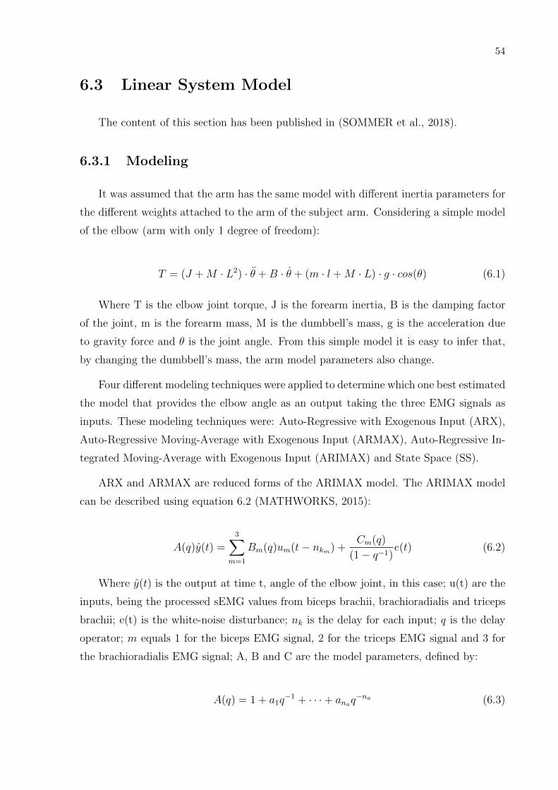
6.3 Linear System Model . . . . . . . . . . . . . . . . . . . . . . . . . . . . . . 54
6.3.1 Modeling . . . . . . . . . . . . . . . . . . . . . . . . . . . . . . . . 54
6.3.2 Results . . . . . . . . . . . . . . . . . . . . . . . . . . . . . . . . . . 55
6.4 Non-Linear System Model . . . . . . . . . . . . . . . . . . . . . . . . . . . 58
6.4.1 Modeling . . . . . . . . . . . . . . . . . . . . . . . . . . . . . . . . 59

6.4.2 Results . . . . . . . . . . . . . . . . . . . . . . . . . . . . . . . . . . 62
6.5 Discussion and Conclusions . . . . . . . . . . . . . . . . . . . . . . . . . . 65
Part IV: TESTING 67
7 Control Testing 68
7.1 Calibration . . . . . . . . . . . . . . . . . . . . . . . . . . . . . . . . . . . 68
7.1.1 Equipment and Materials . . . . . . . . . . . . . . . . . . . . . . . 68
7.1.1.1 EMG sensor . . . . . . . . . . . . . . . . . . . . . . . . . . 68
7.1.1.2 Microprocessor . . . . . . . . . . . . . . . . . . . . . . . . 69
7.1.2 Subjects and experimental setup . . . . . . . . . . . . . . . . . . . 69
7.1.3 Experimental protocol . . . . . . . . . . . . . . . . . . . . . . . . . 70
7.1.4 Experimental data processing . . . . . . . . . . . . . . . . . . . . . 70
7.1.5 Modeling . . . . . . . . . . . . . . . . . . . . . . . . . . . . . . . . 70
7.2 Testing . . . . . . . . . . . . . . . . . . . . . . . . . . . . . . . . . . . . . . 71
7.2.1 Data processing . . . . . . . . . . . . . . . . . . . . . . . . . . . . . 71
7.2.2 Results . . . . . . . . . . . . . . . . . . . . . . . . . . . . . . . . . . 72
7.3 Discussion and Conclusions . . . . . . . . . . . . . . . . . . . . . . . . . . 74
Part V: DISCUSSIONS, CONCLUSIONS AND FUTURE WORK 75
8 Discussions and Conclusions 76
9 Future Work 79
References 81
Appendix A – ETMICAE Calculations, Simulations and Materials 88
A.1 Hip . . . . . . . . . . . . . . . . . . . . . . . . . . . . . . . . . . . . . . . . 88
A.1.1 Applied Forces . . . . . . . . . . . . . . . . . . . . . . . . . . . . . 88

A.1.2 Materials . . . . . . . . . . . . . . . . . . . . . . . . . . . . . . . . 88
A.1.3 Calculations and simulations . . . . . . . . . . . . . . . . . . . . . . 89
A.2 Knee . . . . . . . . . . . . . . . . . . . . . . . . . . . . . . . . . . . . . . . 90
A.2.1 Applied forces . . . . . . . . . . . . . . . . . . . . . . . . . . . . . . 90
A.2.2 Materials . . . . . . . . . . . . . . . . . . . . . . . . . . . . . . . . 93
A.2.3 Calculations and simulations . . . . . . . . . . . . . . . . . . . . . . 93
Appendix B – Actuator Control 94
B.1 Exoskeleton Model . . . . . . . . . . . . . . . . . . . . . . . . . . . . . . . 94
B.1.1 Exoskeleton . . . . . . . . . . . . . . . . . . . . . . . . . . . . . . . 94
B.1.2 Modeling . . . . . . . . . . . . . . . . . . . . . . . . . . . . . . . . 95
B.2 Control . . . . . . . . . . . . . . . . . . . . . . . . . . . . . . . . . . . . . 97
B.2.1 General Characteristics . . . . . . . . . . . . . . . . . . . . . . . . . 97
B.2.2 Impedance Control . . . . . . . . . . . . . . . . . . . . . . . . . . . 97
B.2.3 Impedance Control Design . . . . . . . . . . . . . . . . . . . . . . . 98
B.2.4 Sliding Mode Control Design . . . . . . . . . . . . . . . . . . . . . . 99
B.3 Simulation Results . . . . . . . . . . . . . . . . . . . . . . . . . . . . . . . 100
B.3.1 Impedance Control . . . . . . . . . . . . . . . . . . . . . . . . . . . 100
B.3.2 Sliding Mode Control . . . . . . . . . . . . . . . . . . . . . . . . . . 101
B.4 Conclusions . . . . . . . . . . . . . . . . . . . . . . . . . . . . . . . . . . . 102
Annex A – Sparkfun Muscle Sensor V3 Schematic 104
Annex B – ModExo Control Hardware Schematics 106

PART I
INTRODUCTION
15
1 INTRODUCTION
In the Introduction it is presented the context and the need for assistive devices along
with a bibliographic review. It presents an historical review on the usage of EMG to
control prostheses and exoskeletons. As a conclusion the goals of this work are detailed.
1.1 Bibliographic Review
In the United States, the number of people between the age of 18 and 64 that has
some kind of movement disability has increased about 12% from 1981 to 2014 (VON-
SCHRADER; LEE, 2017). In Brazil, about 13 million people has some kind of motor
disability (IBGE, 2012). Two of the main disability causes are stroke and spinal cord
injury. Yearly, 15 million people suffer stroke. From these, 5 million are fatal and 5
million cause a permanent disability. These number have been increasing in recent years
and studies indicate they will increase even further (MACKAY et al., 2004). From 250
thousand to 500 thousand people suffer spinal cord injury yearly. The three main causes
of spinal cord injury are traffic accidents, falls and violence. Moreover, with the rising in
life expectancy of the world population (WATKINS, 2005), the number of people affected
by disabilities that difficult movement also raised.
Due to these factors, there is a growing need for mechanisms that assist human move-
ments. One of these mechanisms is the robotic exoskeleton.
Robotic exoskeletons are electromechanical structures coupled to the human limbs,
capable of doing or assisting movements. A robotic exoskeleton is usually composed of
joints and rigid bodies (PONS, 2008). One of the major problems of exoskeletons is the
user’s intention identification. There are several biological signals that can be used to
control an external device. For exoskeleton control, that has the goal of moving a certain
limb, it is interesting to use the same signals that are used to control the human motion,
like the neural control signals responsible to activate the muscles. Since these signals
cannot be accessed directly, the use of electromyography (EMG) has been explored to

16
control these devices.
The surface electromyography (sEMG) signal represents the electrical activity gen-
erated by the motor units of the muscles as a response to the activation provided by
innervating motor neurons and measured on the skin surface. The information present in
the EMG signals is a composition of the synaptic inputs received from the motor neurons
and the electrical properties from the muscle fibers (FARINA; MERLETTI; ENOKA,
2014).
There are several other approaches to the control of a mechanical limb apart from
the EMG signal. Among the relevant methods, some have been used in combination with
EMG for the control of the prostheses or orthoses. These approaches will be described in
section 1.2.2.
1.1.1 EMG Control
In 1955, Battye and colleagues (BATTYE; NIGHTINGALE; WHILLIS, 1955) first
proposed the use of proportional EMG control. The authors developed an apparatus
capable of performing open and close actions so that the test subject could perform a
grasping task. The apparatus consisted of electrodes attached to the skin of the forearm,
an electrical amplifier, a discriminator, which powered a solenoid when input signal was
detected. The solenoid activated a hook, closing it. As a result, the authors were capable
of designing a control system sensitive enough to close, and remain closed, when the test
subject gripped a pencil in the fingers, regardless of the movement of other limbs. They
concluded that the signal captured by the apparatus successfully eliminated the EMG
signal from other muscles.
In 1965, Bottomley et al. (BOTTOMLEY, 1965) proposed another method for EMG-
driven prostheses control. Two EMG electrode channels were placed on the forearm, one
on the hand extensors and another on the hand flexors, to measure the muscle activity.
The signal from the muscles were amplified, rectified and smoothed. To remove the
“cross-talk”, that is, the influence of the neighbor-muscle signals on the targeted muscle
signals, the signal of the neighbor muscle was subtracted from the signal obtained from
the target muscle. These signals were used to control a Split hook capable of grasping
objects, that exerted a force proportional to the EMG signal intensity. To control the
desired force, a force sensor was attached to the hook. This device included a feedback
control system that was capable of increasing or decreasing the Split hook grasping force
based on the measured EMG signal. When the force sensor detected zero force, that

17
is, the hook is not grasping the object anymore and it is freely moving, the intensity of
the EMG signal controlled the hook speed. A backlash generator was introduced in the
electrical system to attenuate random variations around a preset threshold, that widens
as the force feedback signal increases. The authors state that, after a few minutes wearing
the apparatus, all the test subjects, even amputees, were able to control the hook in a
graded manner (BOTTOMLEY, 1965).
Also in the sixties of the last century, Alter (ALTER, 1966) designed an exoskeleton
control using two differential electrodes, one on the biceps and one on the triceps. Both
signals were rectified and then the triceps signal was subtracted from the biceps signal
and fed to an adjustable low-pass filter. This signal was used as input signal to a power
amplifier driving an electric motor. Strain gauges were attached to the exoskeleton to
measure the force measurement, and this signal entered the system as a feedback signal.
In 1966, Isidori and Nicolo (ISIDORI; NICOLO, 1966) first described the myopulse
processing technique, which was later developed by Childress et al. (CHILDRESS; HOLMES;
BILLOCK, 1971) and Philipson (PHILIPSON, 1985). The myopulse processor works as
follows: when the absolute value of the EMG exceeds a predetermined threshold value,
the processor output is turned on. When the EMG activity increases, the duty cycle of
the myoprocessor output also increases. An illustration of this method can be seen in
figure 1.
In this system, two sets of electrodes were placed over the targeted muscle where the
detection of electrical signal was desired. The EMG signal was sent to the myopulse pro-
cessor, where the input signal was amplified and transformed into Pulse Width Modulated
(PWM) signal. This PWM signal was sent to the microcomputer. Then, the microcom-
puter processed the PWM signals and sent the output signals to control the prosthetic
arm according to the control algorithm. The myopulse processor is an electrical circuit
composed of a dual comparator, with the value of the resistors defining the threshold
value δ.
The EMG signal is analog, since it is a measure of the electrical activity of the muscle.
To use this signal in a digital controller it should be digitized. However, a major advantage
of the myopulse processor is that there is no need for a conventional analog-to-digital
converter. The author also implemented a classification method for the control of a
prosthesis. Differently from the previous control methods, where the joint actuation was
proportional to the intensity of EMG signal, this system can perform different movements.
In this work, by measuring the intensity of EMG signals from two electrode sets, the author

18
Figure 1: Illustration of the myopulse processing technique. The upper trace shows atypical bandpass-filtered EMG signal recorded with surface electrodes. The output willremain off as long as the absolute value of the EMG signal in the upper trace is belowthe level δ, otherwise the output will be turned on. The lower trace illustrates the outputfrom the myopulse processor (Source: PHILIPSON, 1985) .
was able to control seven different states. Figure 2 shows the proposed dynamic area for
the prostheses control. Considering the intensity of the input from the two target muscles
one of the seven possible states is performed, according to the corresponding area on the
dynamic area (PHILIPSON, 1985). This control system was applied to a prostheses and
tested on four amputee volunteers. With proper training sessions, the volunteers were
able to perform some daily tasks such as grasping a plastic cup containing water, pouring
the desired amount and then releasing the cup. In the case of the non-amputees, the
subjects could achieve good control over the seven-state control system.
In 1977, Parker et al. (PARKER; STULLER; SCOTT, 1977) sought to develop a
EMG signal processor for a prosthesis with a minimal error in the identification of the
desired action. The authors developed a model that extracts the relevant information
from the myoelectric signal obtained by a bipolar electrode configuration. One of the main
strengths of this model is that the pooled motor unit firing rate reflects the contraction
level and is thus the information parameter in the myoelectric signal. In 1980, Hogan
(HOGAN; MANN, 1980a, 1980b), also in search of a better myoprocessor, developed a
similar mathematical model to estimate muscle force based on EMG signal.

19
Figure 2: Diagram showing the possible movement areas according to the muscle inputs(Source: PHILIPSON, 1985) .

20
The myoelectric signal can be modeled as a zero-mean stochastic process. In order to
estimate the user’s control signal, it is necessary to add a nonlinearity to the estimator.
Typically, a full-wave rectifier is used for this nonlinearity, followed by a low-pass filter.
Evans et al. (EVANS et al., 1984) proposed another model based approach to this EMG
control problem. The authors used a logarithmic nonlinearity, followed by a a linear
minimum mean-square error in the EMG-force estimation. In this way a Kalman filter
was inserted to estimate the control signal.
Hudgins (HUDGINS; PARKER; SCOTT, 1993) proposed a control strategy for a
multifunction prosthesis based on the classification of myoelectric patterns into different
movements. Initially, the author conducted tests on both healthy subjects and amputees.
The test consisted of an isometric and isotonic contraction and a contraction (e.g. flexion,
extension, etc.) with no constraints related to force, velocity or range. The subjects were
asked only to make consistent motions, starting from a comfortable neutral position.
By taking the average of the EMG signal for the first 300ms to 600ms of the movement,
that is the onset, it was possible to detect different signal patterns for each movement,
shown in figure 3. Other control schemes, based on steady state levels, are limited to only
three limb functions: for an elbow mechanism, one can only control extension, flexion
and the off-state. The scheme proposed by Hudgins targets the EMG signal of only one
muscle and is capable of assigning as many functions as the number of distinct signal
patterns generated by the muscle.
Since the prosthesis is capable of performing different movements, it is necessary to
implement a classifier that chooses the desired movement or action based on the input
signal. An Artificial Neural Network (ANN) was chosen as the classifier. The authors
proposed a group of parameters, called features, which served as input to the classifier.
The following features were chosen to represent the myoelectric patterns: Mean Absolute
Value (MAV): it is the mean value of the rectified signal throughout the data segment;
Mean Absolute Value Slope: is the difference, in value, between the MAV of each segment;
Zero Crossing (ZC): number of times the waveform crosses the zero value (a ”dead-zone”
must be introduced to avoid noise inducted zero crossings); Slope Sign Changes (SSN): the
number of times the slope of the waveform changes sign (the same ”dead-zone” applied
previously must be applied here); Waveform Length (WL): is the cumulative length of
the waveform throughout the data segment. By using these previous features, one can
get values for waveform amplitude, frequency and duration. This classification method
has become known as the Time Domain feature set (NIELSEN et al., 2009).

21
Figure 3: Average of the first 300ms of the EMG recordings for the following movements:For a healthy subject: a) Isometric contraction; b) elbow flexion; c) Forearm supination;d) elbow extension; e) wrist flexion; f) forearm pronation; for the amputee subject: g)inward humeral rotation; h) contraction of the flexor muscle group; i) contraction of theextensor muscle group and j) biceps/triceps co-contraction (Adapted from HUDGINS;PARKER; SCOTT, 1993).

22
The tests showed that the subjects were capable of performing up to four different
movements with an accuracy ranging from 70-95%, before training. However, a major
drawback from this control scheme is that, since the classification method only considers
the movement onset, the EMG signal must always start from a resting position. If the
user tries to switch from one movement to another in a period of time smaller then the
averaging window (300ms-600ms), the control scheme will fail.
Englehart (ENGLEHART et al., 1999), further developing the pattern recognition
problem, tested some time-frequency-domain sets for the EMG signal processing. The
sets used were: Short-time Fourier Transform (STFT), Wavelet Transform (WT) and
Wavelet Packet transform (WPT).
The same group also proposed a method to overcome the previous problem regarding
the fast transition between two different movements (ENGLEHART; HUDGINS, 2003).
To do so, instead of segmenting the EMG data into multiple frames for classification, now
the data was acquired continuously on a single, unsegmented window. In this scenario,
the data acquired from 12 subjects were compared using the Time Domain statistics and
using the time-frequency-domain sets. The Time Domain sets outperformed the time-
frequency-domain sets in continuous data acquisition.
Jiang (JIANG; ENGLEHART; PARKER, 2009) proposed a method to estimate force
from the Mean Square Value (MSV) of the EMG signal. MSV is defined as the mean value
of the square of the signal throughout the data segment. By stating that it is possible to
maintain the muscle cross-talk at low levels, it is possible to determine a direct relationship
between muscle force and sEMG measurements.
In 2013, Aung, Al-Jumaily (AUNG; AL-JUMAILY, 2013) proposed a method to es-
timate an upper limb joint angle using a back propagation neural network (BPNN) inte-
grated into a Virtual Human Model (VHM). EMG data from anterior deltoid, posterior
deltoid, biceps brachii and triceps brachii were recorded and used as input to the model.
The applied neural network was composed of three layers: input layer, using the EMG
signal from the four arm muscles; hidden layer using Levenberg-Marquadt algorithm; and,
finally, the output layer.
In 2016, Rahmatian et al. (RAHMATIAN; MAHJOOB; HANACHI, 2016), using
a Support Vector Machine (SVM) algorithm associated with a Time-Delayed Artificial
Neural Network (TDANN), proposed a method for continuous estimation of ankle joint
angle. The authors used sEMG data from tibialis anterior, gastrocnemius medialis and
gastrocnemius lateralis muscles. The SVM algorithm was used for classification of sEMG

23
while the TDANN approximated angles and velocities of the ankle joint. The authors
achieved an accuracy of 95.4% for the classification procedure.
Also in 2016, Mamikoglu et al. (MAMIKOGLU et al., 2016) proposed a method
to estimate ankle joint angles based on muscle modeling and the measurement of EMG
signals. The model is based on a multiple input, single output (MISO) Autoregressive
Integrated Moving-Average with Exogenous Input (ARIMAX) model, using integrated
EMG measurements as input and estimating the corresponding joint angles. The proposed
method was capable of achieving fitness values above 0.9 for single speed contractions and
above 0.77 for varying speed contractions.
The addition of a load can decrease the accuracy of EMG-based control systems
up to 60% (AL-TIMEMY et al., 2013). To address this problem, in 2017, Azadet et al.
(AZAB; ARVANCH; MIHAYLOVA, 2017) acquired EMG data from three subjects, using
four different loads and used them for training a k-Nearest Neighbors algorithm (KNN)
and Naive Bayes classifiers (NB). The results showed mean accuracy of 53% and 36%,
for KNN and NB respectively, for subject-dependent conditions, and 22% and 36% for
subject-independent conditions.
1.1.2 Hybrid Control and Other Control Modalities
Hybrid control refers to a group of controllers that combine the information from
different sources in order to perform the control of the mechanism.
1.1.2.1 Hybrid Control
If the subject had some residual shoulder movement it is possible to combine a joy-
stick at the shoulder with EMG for a movement classification method (LOSIER; ENGLE-
HART; HUDGINS, 2007). The system was capable of performing nine different activities.
Eight of then were controlled by the position of the shoulder and one by EMG input when
the user performed a humeral rotation movement. The Time Domain technique was used
to differentiate the EMG readings from humeral rotation from the normal shoulder move-
ments.
Fougner and Stadvahl (FOUGNER et al., 2008; STAVDAHL et al., 2011) used force
sensors on the EMG electrodes to measure external forces. This application is useful for
the cancellation of artifacts caused by these forces (e.g. movement artifacts).
Fougner (FOUGNER et al., 2011) noted that different limb positions associated with

24
daily activities can affect the EMG signal results. To overcome this problem, the EMG
signal was associated with accelerometers placed at the user’s forearm and biceps. This
allows the pattern recognition system to know the position and orientation of the limb,
compensating for eventual changes on the EMG signal.
1.1.2.2 Other Control Modalities
If EMG sensors are difficult to place or if they cause discomfort to the user other
techniques such as Mechanomyography (MMG) may be used. Mechanomyography is the
measurement of the mechanical vibrations caused by the contraction of the muscle. In
Silva (SILVA; CHAU; GOLDENBERG, 2003), the MMG sensors were used as a substitute
of the EMG sensors, when the EMG sensors are of difficult placement or unconfortable
for the patient. This method can also be referred as phonomyogram, vibromyogram,
soundmyogram or acoustomyogram, since the sensor is composed of an accelerometer and
a microphone that detects the air vibration between the sensor and the target muscle.
Kenney (KENNEY et al., 1999) used the dimensional change of the muscle as control
signal for his control strategy. This technique is called Myokinemetric. The author
designed a sensor, composed by a Hall Effect sensor and a permanent magnet. The relative
distance between these two components varied according to the dimensional change of the
subject’s muscle. To validate this strategy a tracking test was performed, where the test
subject was supposed to track a signal presented on a screen by controlling the dimensions
of his muscle.
Stadvahl (STAVDAHL; GRONNINGSAETER; E.MALVIG, 1997) used ultrasound to
estimate the muscle force. As the muscle contracts, the shape of the muscle changes. The
ultrasound, when transmitted to a medium, generates an echo signal that can be acquired
with a sensor. Using this information, a relation between ultrasound and force signals can
be determined by the Cross Correlation technique. Chen (CHEN; CHEN; DAN, 2011)
attached ultrasound transducers to the subject’s forearm to estimate the wrist angle using
the ultrasound signal.
Nightingale (NIGHTINGALE, 1985) used force and slip sensors on the Southampton
Hand to detect forces applied to the hand and relative slipping motion between the hand
and objects. By using the force and slip sensors paired with an EMG control, a state
machine controller was implemented. According to the EMG signal magnitude the control
logic would open or close the hand and by using force sensor measurements, more specific
states for the hand movement, like holding or squeezing an object were accessed.

25
1.1.3 State-of-the-Art of Exoskeletons and Exoskeleton Control
The exoskeletons can be grouped as a function of their applications: performance
enhancement, haptic interfaces, remote operation, functional assistance (active orthoses
and prostheses), rehabilitation and motor control exploration. In this work two groups
will be focused on: the performance enhancement and the functional assistance. The
performance enhancement exoskeleton allows healthy users to perform a difficult task by
either reducing the forces or the expended energy, or perform a task that is impossible to
accomplish by human strength or skill, solely. The functional assistance assists the user
by modifying or recovering the motor function of the neuromuscular and skeletal system.
However, this distinction, in some cases, can be not as clear (DOLLAR; HERR, 2008).
One of the major incentives to the development of exoskeleton has been the Exoskele-
tons for Human Performance Augmentation (EHPA), a program supported by the Defense
Advanced Project Agency (DARPA), an agency of the United States Department of De-
fense. This program is developing exoskeletons capable of increasing the capabilities of
ground soldiers beyond that of a human. There are three critical technologies that are
the focus of this program: Energy, power and actuation; controls and haptic interface;
design and integration (GARCIA; SATER; MAIN, 2002).
HAL (Hybrid Assistive Limb) is an exoskeleton focused on both performance-augmenting
as well as rehabilitation (SANKAI, 2011). The HAL-5 is a full-body exoskeleton. The
joints are powered by DC motors with harmonic drives placed directly on the joints. The
exoskeleton is attached to the user by harnesses at the hip, thighs, calves, upper arms
and forearms, as well as the shoe that is equipped with ground reaction force sensors.¡.
The HAL-5 utilizes a broad range of sensors for its controller. The intention detection
is done primarily by sEMG sensors. As soon as the EMG level exceeds a threshold, the
motion support is triggered. An assistive torque is provided to the user. This torque
is composed of three parts: an assistive torque; a viscous torque that prevents high
velocities, maintaining safety; and a gravity compensating torque (KAWAMOTO et al.,
2010). In some experiments, the motion intention detection was done by the ground
reaction sensor, to adapt the exoskeleton for patients with spinal cord injury. When the
user shifts its weight to the next stance leg, the reaction force on this leg is higher than
the other, triggering the exoskeleton motion (TSUKAHARA et al., 2015). Also, there are
potentiometers, gyroscopes and accelerometers for the measurement of the angle, speed
and acceleration of limbs and joints.
In (OTSUKA et al., 2011) the authors further developed the HAL upper-limb ex-

26
Figure 4: HAL-5 exoskeleton (Source: SANKAI, 2011) .
oskeleton for meal assistance. It is composed of a shoulder joint with three degrees of
freedom and an elbow joint with one degree of freedom. Also, a grasp assistance mecha-
nism is attached to the forearm to allow for manipulation of objects by the user.
One interesting aspect of the HAL exoskeleton is its modularity. Currently, there
are separated products for upper-limbs, lower-limbs, lumbar support, as well as other
modalities, like a heavy-duty and a disaster recovery exoskeleton (CYBERDYNE, 2007).
The manufacturer states that the full-body HAL-5 weighs approximately 23kg, has
a continuous operating time of approximately 2 hours and 40 minutes and is capable
of lifting objects up to 70kg. The HAL R© exoskeleton is capable of performing different
activities such as standing up from a chair, walking and climbing up and down stairs.
The HAL R© exoskeleton is already used in many medical institutions in Japan and
already received certification for clinical use in Europe. It is commercialized by Cyberdyne
Inc.
The Berkeley Lower Extremity Exoskeleton (BLEEX), funded by the DARPA, is a
self-powered exoskeleton that enhances the strength and endurance of a human (KAZE-
ROONI, 2006).
The BLEEX exoskeleton has 7 degrees of freedom (DOF) per leg: 3 DOF at the hip,
1 DOF at the knee and 3 DOF at the ankle. For the hip, both the flexion/extension and

27
Figure 5: University of California at Berkeley’s BLEEX exoskeleton (Source: ZOSS;KAZEROONI; CHU, 2006) .
the abduction/adduction joints are aligned to the human joint, but the rotation joint is
positioned behind the user and under the torso. The reason is that an aligned rotation
joint would result in limited ranges of motion and singularities in some of the human
postures. For the ankle, the flexion/extension axis coincides with the human ankle joint,
but the abduction/adduction and rotation axes do not coincide with the human joint
axes and form a plane outside of the human’s foot. However, the forefoot is compliant,
allowing the toe flexion. The exoskeleton is only rigidly connected to the user at the hip
and the foot (ZOSS; KAZEROONI; CHU, 2006).
The BLEEX structure and actuation was designed based on the clinical gait analysis
(CGA) of an 75-kg person. Analyzing the CGA, it was possible to determine which
exoskeleton joint required actuation, based on the joint torque and power during gait.
From this analysis, it was determined that the flexion/extension joints of hip, knee and
ankle and the abduction/adduction joint of the hip should be actuated.
Initially, the selected actuator for the BLEEX was a double-acting linear hydraulic
actuators. These actuators are compact in size, low weight and capable of exerting high
forces. They are placed in a triangular disposition in relation to the joint, resulting in a
torque that varies according to the joint angle (CHU; KAZEROONI; ZOSS, 2005).

28
The average power consumption of the BLEEX during the walking cycle is 1143 W,
compared to 165 W of mechanical power exerted by the human during normal gait. This
exoskeleton is capable of supporting up to 75 kg and walk at speeds up to 1.3 m/s.
In a later study, the feasibility of using electrical motors instead of the previous
hydraulic ones was analyzed. The designed electrical motors weighed an average of 4.1
kg opposed to the 2.1 kg hydraulic actuators. While the electric actuator weight is all
centered in the actual joint, about 40% of the weight hydraulic actuator is located away
from the joint. At test performed at ground-level walking at the speed of 1.3 m/s, it was
measured that the actuator power consumption was 598 W. Comparing both actuators,
the electrical actuator is 95% heavier and 92% more power efficient (ZOSS; KAZEROONI,
2006).
An hybrid Hydraulic-Electric Power unit (HEPU) was designed in the attempt to
provide autonomous energy for the exoskeleton. The hydraulic energy would supply the
necessary mechanical parts of the exoskeleton, while the electrical energy would power
the computer, sensors and other peripherals. Even though the designed HEPU could
provide the necessary requirements of electrical and hydraulic power, it exceeded in both
weight and noise output. The desired weight and noise output were 23 kg and 78 dBA,
respectively. The achieved values were 30 kg and 87 dBA (AMUNDSON et al., 2006).
The control of the BLEEX exoskeleton has no sensors attached to the user. Every sen-
sor is located only on the exoskeleton. It uses the forces applied by the environment and
the user to the exoskeleton as the control signal (STEGER; KIM; KAZEROONI, 2006).
The inverse dynamics of the exoskeleton is used as a feedback so that, when account-
ing for the user force, the control loop gain approaches an unitary value. This control
strategy has two main advantages: it allows for wide bandwidth maneuvers, necessary
since the exoskeleton needs to respond to a wide variety of the human’s movements; it is
independent to changes in the user dynamics. The trade-off of this control strategy is that
it needs an accurate model of the exoskeleton dynamics. To address this, experiments
in (GHAN; KAZEROONI, 2006) applied system identification methods to calculate the
exoskeleton dynamics.
One of the most well-established exoskeletons for disabled users is the ReWalkTM.
The ReWalkTM is a lower extremity, battery powered exoskeleton that allows individuals
with thoracic or lower level motor complete spinal cord injury to walk independently. It is
suitable for adults who have preserved bilateral upper extremity function. The user must
be using crutches to maintain balance. The mechanical structure is composed of bilateral

29
supports parallel to the thighs and legs, articulated at the knee and hip. A rigid shoe
insert fixes the user’s feet. Velcro closures distributed at the legs and thighs and a waist
belt secure the attachment between user and exoskeleton. The computer-based controller
and the batteries are stored within a backpack. A tilt sensor is placed at the exoskeleton
structure, near the waist (ESQUENAZI, 2013).
The active joints of the ReWalkTM are the knee and waist joint. The ankle joint is
passive joint with spring-assisted dorsiflexion. The exoskeleton has five different operation
modes: walk, sit-stand, stand-sit, up steps and down steps. In the ’walk’ mode, the
stepping procedure is triggered by the forward flexion of the upper body, measured by
the tilt sensor. The maximum walking velocity is 2.2 km/h. The mode selection can be
made through an user-operated wrist pad. There is also the option to manually control
the position of the lower limbs (ZEILIG et al., 2012).
Figure 6: The ReWalkTM exoskeleton worn by an user and its basic structure (Source:ESQUENAZI, 2013) .
Some studies have been performed with the ReWalkTM (ZEILIG et al., 2012; FINEBERG
et al., 2013; TALATY; ESQUENAZI; BRICENO, 2013). Overall, the participants of the
test were satisfied with the device, being able to walk without falling. The volunteers
reached the level of being able to walk 100m with the use of crutches. However, they
have not attained proficiency to use the device on a daily basis. It is stated that the users
found relative difficulty with wearing and adjusting the device.
30
Even tough many advancements in this area have been made, the effective use of an
exoskeleton continues to be extremely difficult. Even though many technologies have been
advertised lately, there is a lack of quantitative studies available to researchers (YOUNG;
FERRIS, 2017).
The MIT exoskeleton, a quasi passive exoskeleton concept, explores the passive dy-
namics of human walking trying to achieve a lighter and more efficient exoskeleton. The
tests showed that the total metabolic cost of walking increased when used the exoskeleton
while carrying a load, compared to no exoskeleton being used while carrying the load in a
backpack. The increase in metabolic cost was found to be 10% higher (WALSH; ENDO;
HERR, 2007). Nevertheless, the participants in the tests stated that carrying the load
while wearing the exoskeleton was more comfortable compared to carrying the backpack
alone (VALIENTE, August, 2005). Another study demonstrated the exoskeleton is capa-
ble of transferring up to 90% of the load to the ground, depending on the gait phase, but
increases the metabolic cost in a range from 32% up to 74%, depending on some variations
of the mechanical structure and actuation of the exoskeleton (WALSH, February, 2006).
It has been previously studied that one of the major problems of ambulation de-
vices for paraplegics is the high-energy demands imposed to the user. Franceschini et al.
(FRANCESCHINI et al., 1997) conducted a survey on patients that utilized reciprocating
orthoses (ARGO, RGO, HGO). From the 74 patients, 24 patients abandoned the use of
the mechanism by the end of the study. One of the main reasons was the excessive energy
cost.
1.2 Objective
The objective of this dissertation is to design the controller of a one-degree-of-freedom
exoskeleton using sEMG signals from the user as the input signals. The controller must
be accurate in replicating the movement desired by the user, as well as requiring little
training from the user.

31
2 METHODOLOGY
The ideal control method would be one that requires no prior training. The user
would be capable of controlling the mechanism as easily as he can control his own limb.
Of course this is an ideal scenario and, as stated in many previous studies already cited
in this work, we are still far from understanding the real dynamics of limbs, muscles and
electromyography signals.
With those challenges in mind, how can we design a control that is capable of con-
trolling a mechanical ”limb-like” mechanism?
One potential idea is to design a control method that mimics the physical charac-
teristics of the human limb, that is, a biomimetic control. Biomimetics is the study of
biological mechanisms and processes with the purpose of synthesizing similar products
and behaviors by an artificial mechanism which mimics natural ones (MERRIAMWEBS-
TERDICTIONARY, 2009). To achieve this biomimetic behavior, the model-based control
method can be a great candidate.
Biomechatronics, control designing and system modeling must be combined to achieve
an EMG-Driven exoskeleton controller that is both safe and natural to user. Therefore,
it is necessary to approach this design in a structured manner.
First, available and in development exoskeleton platforms at the Biomechatronics
Laboratory at Escola Politecnica of the University of Sao Paulo (USP) will be analyzed in
respect to its mechanical and electronic design, as well as its sensoring, to better determine
the one that is more appropriate for the application of the EMG-driven controller.
An experimental procedure will be conducted to obtain EMG and angle data of a
predetermined movement, for the design of the controller.
Two different EMG-to-Angle model estimation methods will be applied and evaluated:
a linear method and a nonlinear method. They will serve as a base for the controller design.
The methods will be compared according to their accuracy, complexity and applicability
in the chosen exoskeleton platform.

32
The controller will be adapted so it can be applied in real time conditions. The
controller undergoes testing in real time conditions to determine if the goals proposed for
this work were achieved.
Finally, the results are discussed and compared to similar works from the literature.
Figure 7 presents a diagram with this structure in a visual manner.

33
Figure 7: Visual representation of framework/methodology

PART II
EXOSKELETON PLATFORMS
In this part, it is described exoskeletons
available and being developed at the
Biomechatronics laboratory that can be
used to implement the control strategies
developed in this work

35
3 TRUNK AND LOWER LIMB EXOSKELETON
FOR STABLE AUTONOMOUS WALKING
(ETMICAE)
3.1 Description
The ETMICAE is a bipedal trunk and lower limb exoskeleton to assist the walking
movement of people with motor disabilities. It allows the use of the exoskeleton by people
that cannot maintain a full control of their body and lower limbs. It includes human gait
stability control.
It is currently being developed at the Biomechatronics Laboratory - Mechanical En-
gineering and Mechanical Systems Department - Escola Politecnica of the University of
Sao Paulo (USP). This project is being developed in collaboration with the Rehabilitation
Medicine Institute of the Clinics Hospital - Medicine School of USP, Sao Carlos School of
Engineering (EESC-USP).
When the project is completed, it will mainly contribute in two major areas: Clinical
studies and technological studies. For clinical studies, the ETMICAE will be transferred
to a clinic to test and evaluate the exoskeleton on subjects with motor disabilities. For
the technological studies, the exoskeleton will act as platform for testing of mechanical,
electrical and control technologies developed at the Biomechatronics laboratory.
3.2 Mechanical Structure
With the goal of using ETMICAE as a platform to test the sEMG controllers, the
author of this dissertation was responsible in designing the hip, thigh, knee and leg me-
chanical structure, as well as its coupling components. The 3D modeling of the exoskele-
ton can be seen in figure 8. The explanation of this design is described in this section.
Calculations for the mechanical design are described in Appendix A.

36
Figure 8: Assemble of the ETMICAE

37
3.2.1 Hip
The hip of the exoskeleton will have four degrees of freedom, being the abduc-
tion/adduction and flexion/extension of both thighs. The exoskeleton will not have the
pronation/supination movement of the thighs.
The hips are composed of the following parts:
A base will will attach the hip of the exoskeleton to the support of the motors, located
at the back of the user.
Figure 9: Base
Attached to the base there are two joints that will perform the abduction/adduction
degree of freedom for the thighs. For this coupling a shaft supported by two ball bearings
will allow the relative movement between the two parts. Between the thigh component
and the base, a low friction thrust washer is inserted to support the axial forces and allow
smooth slipping. Another thrust washer is positioned at the external part of the joint to,
in conjunction with an aluminum cover, support the axial forces.
Figure 10: Hip abduction/adduction joint
Linked to these joint, a folded aluminum plate extends to the next hip joint.
The lateral joint allows for the flexion/extension degree of freedom of the thighs. This
joint is also composed by a shaft supported by two ball bearings with a thrust washer

38
Figure 11: Hip plate
between the two parts.
Figure 12: Hip flexion/extension joint
3.2.2 Knee
Each knee will have only one degree of freedom, aligned to the flexion/extension joint
of the user. It is constituted of the following parts:
A bar that extends from the flexion/extension joint of the hip to the knee joint. This
bar stays parallel to the user’s thigh.
Attached to the thigh bar, a rotation joint allows the flexion/extension movement of
the mechanism. At this joint a shaft supported by two ball bearings will be used. Between
the two parts of the joint a low friction coefficient thrust washer is positioned to support

39
(a) Thigh (b) Leg
Figure 13: Thigh and leg bars
the axial forces and allow for smooth sliding between the parts. Another thrust washer
is positioned at the external part of the joint, along with a metallic cover, to support the
axial forces.
Figure 14: Knee flexion/extension joint
Attached to this joint, another metallic bar extends to the ankle.

40
4 UPPER LIMB EXOSKELETON WITH ONE
DEGREE OF FREEDOM (ULEXO)
This chapter briefly describes an upper limb exoskeleton with one degree of freedom
already available at the Biomechatronics laboratory. This system was first designed in
(SOMMER, 2015).
4.1 Mechanical
4.1.1 Structure
The exoskeleton structure is made of aluminum bars. The aluminum structure is
attached to a Power Window Lifter steel mechanism.
The user’s arm is placed at the aluminum structure and held firmly through the use
of rubber straps.
Figure 15: Upper limb exoskeleton with one degree of freedom (Source: SOMMER, 2015).

41
4.1.2 Actuator
The actuator of the exoskeleton is composed by a (578VA, Mabuchi Motor Co., ltd.,
Japan) DC motor and a Power Window Lifter mechanism.
This DC Motor was chosen because of its high power-to-weight ratio, low dimensions
and low price.
In order to increase the motor torque, the DC motor is attached to a modified Power
Window Lifter, a mechanism with gear coupling with a reduction factor of 10:1. Modeling,
Impedance Control and Sliding Mode Control studies have been conducted with this
exoskeleton and are presented in Appendix B
Figure 16: Power Window Lifter (Source: SOMMER, 2015) .
4.2 Electronics
The electronics system of the exoskeleton is composed of the following parts: An
sEMG sensor, that acquires the sEMG signal of the biceps muscle; a microprocessor to
process the analog sEMG signal, apply the control logic and output a PWM signal; a
motor driver that receives the PWM signal as input and outputs the necessary power to
drive the DC motor.

42
Figure 17: Schematic of the electronics (Source: SOMMER, 2015) .
4.2.1 EMG Sensor
The EMG Sensor is (Muscle Sensor V3, Sparkfun Electronics R©, USA).
Three electrodes are attached to this sensor: Two electrodes are placed at the target
muscle and measure the difference of electrical activity and one is placed at an electrically
neutral region of the body, like a bony area, and serves as the ground signal.
The signal from the electrodes is differentially amplified in the AD8221 amplifier; then,
the signal is amplified twice by TL084 operational amplifiers; the signal is rectified using
1N4148 diodes; the rectified signal is attenuated by a filter with 2Hz cutoff frequency; at
last, the signal is amplified with an adjustable gain.
The Sensor output is sent directly to the microprocessor.
4.2.2 Microprocessor
The microprocessor is an (Arduino UNO, Arduino, S.r.l., Italy). It was chosen for
its low cost, ease-of-use, extensive available documentation and easy communication to
the Muscle Sensor V3. It has a built-in 10-bit resolution Analog/Digital converter and
is capable of emitting PWM signals. Also, it is possible to connect more sensors to this
microprocessor, for future adaptations of the exoskeleton.

43
4.2.3 Driver
The DC motor demands electrical currents up to 24A. Motor Drivers for 12V, 24A
DC motors are expensive. For this reason, a motor driver was designed for the specific
use on this exoskeleton.
The driver has two inputs (clockwise rotation and counter-clockwise rotation) that
receives the PWM signal from the microprocessor for the desired direction of motion.
There are two outputs that are connected to each one of the motor electrical terminals.
The driver is composed of a H-Bridge of MOSFETs. The chosen components were
IRF4905 for P channel and IRLB3813 for N channel. The gate of the P channel MOSFET
is powered by a TIP122 transistor.
To avoid the situation where every MOSFET of the H-Bridge is activated at the same
time, which would cause a short circuit between the poles of the battery, a protection
circuit was implemented. The protection circuit is composed of 74LS08 AND gates and
74LS04 NOT gates. In case both the inputs are powered, no signal reaches the gates of
transistors, protecting the circuit.
This exoskeleton has some limitations, since it does not contain angular sensors, has
limited speed control and requires extensive work for a feedback controller to be imple-
mented.

44
5 MODEXO
This chapter briefly describes a development platform for exoskeleton research avail-
able at the Biomechatronics laboratory. The system was first presented in (SOUZA,
2018)
5.1 Mechanical
5.1.1 Structure
The ModExo is an exoskeleton development platform. It replicates one degree-of-
freedom of an exoskeleton, coupling a motor to a load cell.
A load cell is attached to the structure of the exoskeleton segment, which provides
contact torque between user and exoskeleton (SOUIT, 2016).
The load cell is designed to deform elastically in a Wheatstone bridge configuration
and measured the force applied to the exoskeleton.
A 3D printed case protects the strain gauges wiring and serves as an attachment to a
forearm support.
The ModExo is assembled in a wooden portable case. The assembly can be seen in
figure 18.
5.1.2 Actuator
The actuator of the ModExo is composed of a flat brushless DC motor (EC90 Flat,
Maxon Motors AG, Switzerland). It has integrated an encoder (Encoder MILE, Maxon
Motors AG, Switzerland), and a harmonic reduction (Harmonic Drive 100:1, Harmonic
Drive, Ltd, Japan)).
The motor was chosen for its high torque-velocity curve. It also offers high power-

45
Figure 18: User testing the ModExo workbench (Source: SOUZA, 2018) .
to-mass ratio and has low dimensions. Because of its flat design, it reduces the torsional
deflection of the motor when placed in parallel with the human body.
5.2 Electronics
5.2.1 Sensors
Strain gauges, assembled in full Wheatstone bridge, attached to the load cell, provide
contact torque information.
5.2.2 Driver
The driver used is also from Maxon (EPOS2 70/10, Maxon Motors AG, Switzerland).
It receives position commands from the central controller and transmits them to the
Maxon motor. It also receives position feedback from the encoder integrated to the
motor.

46
5.2.3 Microprocessors
A microcontroller based on the (Arduino UNO, Arduino, S.r.l., Italy) acts as a high
level controller, implementing the impedance control and position output for the Maxon
motor.
A CAN bus shield (CAN bus Shield, Seedstudio, China) is used as a CAN bus inter-
face, managing communication between the the microcontroller, EPOS driver and ampli-
fication board. It is connected to the microcontroller as a shield.
5.3 Discussion
The ModExo can be used as a platform that imitates the elbow joint in an upper limb
exoskeleton. Since it has position sensors already implemented, an easy-to-use communi-
cation between a personal computer and the platform, and the possibility to implement
different control methods, it is the best candidate between the three exoskeleton platforms,
to implement the control method designed is this work.
With the exoskeleton platform determined, it is necessary to design the controller for
EMG-to-Angle relation. In the next chapter, the controller design is described.

PART III
CONTROLLER DESIGN
In this part, control methods for the EMG
are proposed and designed to be imple-
mented in an exoskeleton platform.

48
6 MODEL-BASED EMG-DRIVEN CONTROL
The content of this section is an extended version of two full papers presented at IEEE
Conferences: EMBC 2018 and BioRob2018 (SOMMER et al., 2018) and (SOMMER;
FORNER-CORDERO, 2018).
There are different electrophysiological signals that can be used to control an exoskele-
ton. Therefore, it seems interesting to use the control signals that are used by the body
to activate the muscles. As these neural control signals are not easily accessible, surface
electromyography has been used as a control signal for upper-limb exoskeletons (LENZI
et al., 2012).
6.1 Control Description
The Model-Based control method utilizes a dynamic model of the body to predict the
dynamic response according to the input given to the model. There are basically three
types of dynamic models: mathematical, system identification and artificial intelligence
models (ANAM; AL-JUMAILY, 2012).
For this work it was chosen the system identification modeling approach. It is often
used because of the difficulty in describing the dynamic model with mathematical equa-
tions. To do so, a set of inputs and outputs are measured experimentally and then an
identification algorithm develops the relationship between the system inputs and outputs.
There are certain assumptions needed to use these models, such as linearity/non-linearity,
model structure and model order.
By using a dynamic model that mimics the user’s limb dynamics, the exoskeleton
will be capable of performing limb-like movements using the sEMG signals as input. A
mathematical system modeling should consider the EMG to muscle force generation and,
afterwards, take into account the different muscle forces around a certain joint along with
the corresponding moment arms and inertial parameters of the segments to obtain the
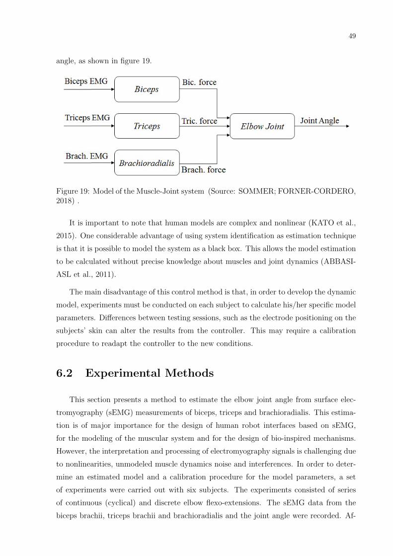
49
angle, as shown in figure 19.
Figure 19: Model of the Muscle-Joint system (Source: SOMMER; FORNER-CORDERO,2018) .
It is important to note that human models are complex and nonlinear (KATO et al.,
2015). One considerable advantage of using system identification as estimation technique
is that it is possible to model the system as a black box. This allows the model estimation
to be calculated without precise knowledge about muscles and joint dynamics (ABBASI-
ASL et al., 2011).
The main disadvantage of this control method is that, in order to develop the dynamic
model, experiments must be conducted on each subject to calculate his/her specific model
parameters. Differences between testing sessions, such as the electrode positioning on the
subjects’ skin can alter the results from the controller. This may require a calibration
procedure to readapt the controller to the new conditions.
6.2 Experimental Methods
This section presents a method to estimate the elbow joint angle from surface elec-
tromyography (sEMG) measurements of biceps, triceps and brachioradialis. This estima-
tion is of major importance for the design of human robot interfaces based on sEMG,
for the modeling of the muscular system and for the design of bio-inspired mechanisms.
However, the interpretation and processing of electromyography signals is challenging due
to nonlinearities, unmodeled muscle dynamics noise and interferences. In order to deter-
mine an estimated model and a calibration procedure for the model parameters, a set
of experiments were carried out with six subjects. The experiments consisted of series
of continuous (cyclical) and discrete elbow flexo-extensions. The sEMG data from the
biceps brachii, triceps brachii and brachioradialis and the joint angle were recorded. Af-
50
ter the model was selected, a second experiment was performed in order to validate the
estimation procedure. The results show an effective model for the EMG-to-angle relation
with great values for both correlation and root-mean-square error when compared to the
measured angle data.
The experimental procedures involving human subjects described in this work were
approved by the Comite de Etica em Pesquisa do Hospital Universitario da Universidade
de Sao Paulo (CEP-HU/USP).
6.2.1 Subjects and experimental setup
Six volunteers (age: 34.3 ± 14.7 years, height: 1.74 ± 0.1 m, weight: 67.9 ± 15.7 kg,
4 male, 2 female, all right-handed) with no known neuromuscular deficit participated in
the experiments. Elbow joint angle along with the surface electromyography (sEMG) of
three right arm muscles, biceps brachii, triceps brachii and brachioradialis were recorded.
sEMG was measured with 3 pairs of (FREEEMG 1000, BTS Bioengineering Corp., Italy)
electrodes with an electrode separation of 20mm with the electrode diameter being 4mm.
A pair of electrodes was placed on the biceps and other pair on the triceps following the
SENIAM guidelines (SENIAM, 2004). To determine the electrode positioning for the bra-
chioradialis muscle, the subject was asked to apply force to flex the forearm while keeping
it at 90◦. Then, the electrode was placed on the belly of the muscle and its respective
pair placed distally at a 20mm following the muscle fiber direction. The sampling rate
was of 1kHz with 16 bit resolution. The user interface was the BTS FREEEMG software
(BTS, Spa, Italy).
To measure the joint angle, a six degrees of freedom Inertial Measurement Unit (IMU,
VN-100 from VectorNav R©, TX, USA), with 0.01◦ precision, was attached on the internal
aspect of the forearm, located at two-thirds distance from the elbow to the wrist. The
angle values were acquired with a rate of 100 samples per second. The data were collected
with Matlab R© (The MAthworks Inc, MA, USA) using a dedicated library provided by
the inertial sensor manufacturer.
The experimental setup can be seen in figure 20.
6.2.2 Experimental Protocol
The subject sat on a chair, with the knees flexed at 90◦, the back perpendicular to
the ground with the scapulas pressed against the wall. The back of the arm was leaning

51
Figure 20: Experimental setup on a test subject (Source: SOMMER; FORNER-CORDERO, 2018) .
against a rubber support that was attached to the wall. This setup guaranteed that the
subject was comfortable enough to perform repeated elbow flexions and extensions while
maintaining the upper arm steady.
The experimental protocol had three parts: The first one consisted of an isometric
force test to obtain the Maximum Voluntary Contraction (MVC). The elbow of subject
was kept in a fixed position at 90◦ and he/she was asked to apply the maximal possible
force to flex the elbow. The subject was given a three minute interval before the next set.
In the second part, the subject was asked to perform five consecutive elbow flexion and
extension movements from 50◦ to 140◦ with a frequency of 0.5Hz, that is, five movements in
ten seconds. To help the subject reach the correct target angles a template was attached
to the wall parallel to the subject, to provide visual guidance. To achieve the desired
movement speed a metronome was set at the speed of 60 BPM so that the subject could
synchronize the movements with the sound of the metronome. A minute of rest was given
to the subject before the next part.
In the third part the subject was instructed to make an elbow flexion for 1 second,
hold his forearm at 140◦ for 1 s, then a 1 s extension movement and then hold the forearm

52
at 50◦ for another 1 s. This cycle should be repeated five times. Another one minute
resting time was given to the subject. Both of the continuous and interval tests were
repeated with 1.5kg and 3kg extra weight placed at the subject’s hand.
No subjects reported fatigue during the experiment.
The test was repeated in a different day, on all test subjects to further analyze the
repeatability of the model proposed in this work.
All the data from the tests were transferred to Matlab R© (The Mathworks Inc, USA).
for further analysis and processing.
6.2.2.1 Experimental Data Processing
The EMG data were processed as follows. Further explanations can be found on the
literature (ROSE, 2011; HAYASHIBE; GUIRAUD; POIGNET, 2009)
1. high-pass filtering of the EMG data, using a 2nd order Butterworth filter, with a
cutoff frequency of 30 Hz, thus removing movement artifact.
2. Wave rectification
3. Second Order low-pass Butterworth Filter, with 1Hz cutoff frequency.
4. normalization with the peak of MVC
This way, the EMG is smoothed and presented as a percentage of the subject MVC
instead of Volts.
A low-pass, 20 Hz cutoff frequency, second-order Butterworth filter is applied to the
angular data to remove errors and other undesired signals.
Since the position tracking data was sampled at 100 Hz while the EMG data was
sampled at 1KHz, all the position tracking data was resampled to 1000 Hz.
Figure 21 shows an example of the recorded elbow angle and processed sEMG for the
continuous movement with no extra weight.
Both the angular data as well as the EMG envelope had to be detrended for the
models estimation.

53
Figure 21: a) Joint angle for the continuous movement with no extra weight, recordedwith the IMU; sEMG values for the b) biceps brachii, c) triceps brachii and d) bra-chioradialis for the continuous movement with no extra weight (Source: SOMMER;FORNER-CORDERO, 2018) .
54
6.3 Linear System Model
The content of this section has been published in (SOMMER et al., 2018).
6.3.1 Modeling
It was assumed that the arm has the same model with different inertia parameters for
the different weights attached to the arm of the subject arm. Considering a simple model
of the elbow (arm with only 1 degree of freedom):
T = (J +M · L2) · θ +B · θ + (m · l +M · L) · g · cos(θ) (6.1)
Where T is the elbow joint torque, J is the forearm inertia, B is the damping factor
of the joint, m is the forearm mass, M is the dumbbell’s mass, g is the acceleration due
to gravity force and θ is the joint angle. From this simple model it is easy to infer that,
by changing the dumbbell’s mass, the arm model parameters also change.
Four different modeling techniques were applied to determine which one best estimated
the model that provides the elbow angle as an output taking the three EMG signals as
inputs. These modeling techniques were: Auto-Regressive with Exogenous Input (ARX),
Auto-Regressive Moving-Average with Exogenous Input (ARMAX), Auto-Regressive In-
tegrated Moving-Average with Exogenous Input (ARIMAX) and State Space (SS).
ARX and ARMAX are reduced forms of the ARIMAX model. The ARIMAX model
can be described using equation 6.2 (MATHWORKS, 2015):
A(q)y(t) =3∑
m=1
Bm(q)um(t− nkm) +Cm(q)
(1− q−1)e(t) (6.2)
Where y(t) is the output at time t, angle of the elbow joint, in this case; u(t) are the
inputs, being the processed sEMG values from biceps brachii, brachioradialis and triceps
brachii; e(t) is the white-noise disturbance; nk is the delay for each input; q is the delay
operator; m equals 1 for the biceps EMG signal, 2 for the triceps EMG signal and 3 for
the brachioradialis EMG signal; A, B and C are the model parameters, defined by:
A(q) = 1 + a1q−1 + · · ·+ anaq
−na (6.3)

55
B(q) = 1 + b1q−1 + · · ·+ bnbq
−nb+1 (6.4)
C(q) = 1 + c1q−1 + · · ·+ cncq
−nc (6.5)
Where na is the number of poles of the system; nb is the number of zeros plus one
and nc is the number of coefficients of the moving average.
In order to find a solution a hard search was done using 1000 models of each type with
random model orders ranging from 1 to 10. A data window of 6s was used to calibrate
the model, while the entire data vector was used to validate the model.
Each model was compared to the reference angle using equation 6.6. The orders of
the model that achieved the highest fitness value were chosen and are presented at table
1. The parameters of the models were estimated using time-domain data in Matlab R©
(The Mathworks Inc, USA).
Fit =
√√√√ ∏3i=1
∏2j=1Corrij∏3
i=1
∏2j=1RMSEij
(6.6)
Where Corrij is the correlation between the measured angle and estimated angle for
each test; RMSEij is the root-mean-square error (RMSE) between the measured angle
and estimated angle (see eq. 6.7); i equals 1 for the 0kg test, 2 for the 1.5kg test and 3
for the 3kg test; j equals 1 for the continuous test and 2 for the intermittent test.
RMSE =√mean((y − y)2) (6.7)
Where y is the measured angle and y is the estimated angle.
6.3.2 Results
Figure 22 compares the different models with measured elbow angle and shows the
fitness value for each data set.
The ARX model outperforms the other models for every subject and every test set.
For this reason it was the chosen model for the subsequent estimation procedures.
The model orders calculated are presented in table 1.

56
Figure 22: Estimated elbow angle using the models responses compared to the elbowangle measured with the IMU. The estimated models were ARX, State Space, ARMAXand ARIMAX (Source: SOMMER et al., 2018) .
The best model is a model with a null value on the auto-regressive part of the equation.
For that reason, the best model is, in fact, a Finite Impulse Response (FIR) model, that
can be considered as a particular case of the ARIMAX model.
The FIR model has the following form, as seen in equation 6.8:
y(t) =3∑
m=1
Bm(q)um(t− nkm) + e(t) (6.8)
Table 1: Model orders for each subject (Source: SOMMER et al., 2018) .
na nb nk
Subject 1 0 8, 2, 2 1, 2, 2Subject 2 0 9, 5, 10 1, 3, 0Subject 3 0 1, 4, 8 5, 0, 1Subject 4 0 8, 8, 1 0, 0, 8Subject 5 0 5, 1, 9 2, 8, 0Subject 6 0 4, 3, 10 3, 0, 0
Using the values from table 1 as the FIR model orders, it was possible to calculate the
model for elbow joint angle using the three sEMG measurements as input and compare
it to the experimentally measured values. As an example, figure 23 shows a comparison
between the calculated and estimated angle, for continuous and intermittent movement.
Using the same model parameters previously calculated, we estimated the response

57
Figure 23: Comparison between the measured angle of the elbow joint and the anglecalculated through the use of the estimated model, for subject 2, with a 1.5kg dumbbell.a) shows the comparison for the continuous movement and b) the comparison for thediscrete movement (Source: SOMMER et al., 2018) .
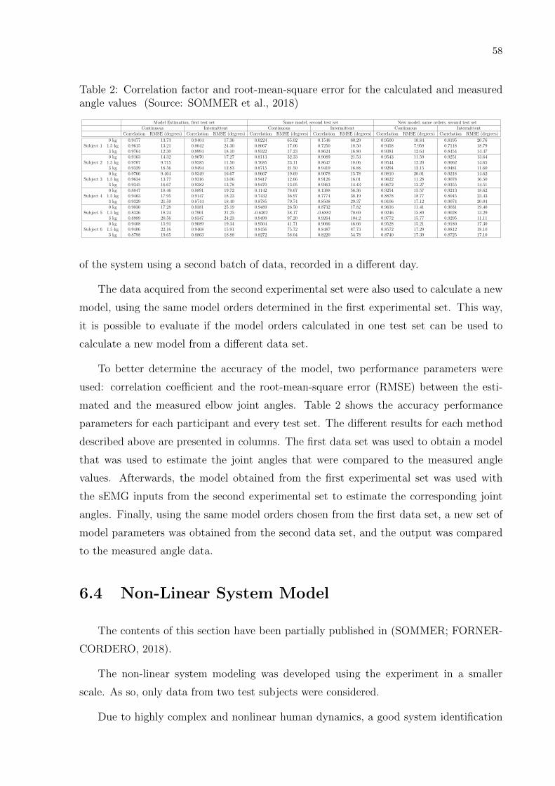
58
Table 2: Correlation factor and root-mean-square error for the calculated and measuredangle values (Source: SOMMER et al., 2018)
Model Estimation, first test set Same model, second test set New model, same orders, second test setContinuous Intermittent Continuous Intermittent Continuous Intermittent
Correlation RMSE (degrees) Correlation RMSE (degrees) Correlation RMSE (degrees) Correlation RMSE (degrees) Correlation RMSE (degrees) Correlation RMSE (degrees)
0 kg 0.9477 13.73 0.9404 17.36 0.0224 65.02 0.1546 60.29 0.9500 10.84 0.8195 20.76Subject 1 1.5 kg 0.9615 13.21 0.8042 24.30 0.8067 17.06 0.7250 18.50 0.9458 7.959 0.7118 18.79
3 kg 0.9764 12.30 0.8994 18.10 0.9322 17.23 0.8624 16.80 0.9381 12.64 0.8454 14.470 kg 0.9163 14.32 0.9070 17.27 0.8113 32.33 0.9089 21.53 0.9543 11.59 0.9251 13.64
Subject 2 1.5 kg 0.9707 9.715 0.9585 11.50 0.7685 23.11 0.8647 18.06 0.9544 12.20 0.9062 14.653 kg 0.9329 18.56 0.9494 12.83 0.8715 21.50 0.9419 16.88 0.9294 12.15 0.9481 11.600 kg 0.9766 9.464 0.9349 16.67 0.9667 19.69 0.9078 15.78 0.9810 20.01 0.9218 14.62
Subject 3 1.5 kg 0.9634 13.77 0.9316 13.06 0.9417 12.66 0.9126 16.01 0.9622 11.28 0.9078 16.503 kg 0.9345 16.67 0.9382 13.78 0.9470 13.05 0.9363 14.43 0.9672 13.27 0.9355 14.510 kg 0.8847 18.46 0.8891 19.72 0.1142 78.67 0.1388 56.36 0.9254 15.57 0.9213 18.62
Subject 4 1.5 kg 0.9463 17.95 0.9147 18.23 0.7432 36.97 0.7774 38.19 0.8878 18.77 0.8045 23.433 kg 0.9329 21.59 0.8744 18.40 0.8785 79.74 0.8508 29.37 0.9106 17.12 0.9074 20.040 kg 0.9030 17.28 0.8381 25.19 0.9489 26.50 0.8732 17.82 0.9616 11.41 0.9031 19.40
Subject 5 1.5 kg 0.8336 18.24 0.7901 21.25 -0.6302 58.17 -0.6882 70.69 0.9246 15.89 0.9028 13.293 kg 0.8989 20.56 0.8347 24.23 0.9499 97.20 0.9264 104.2 0.9772 15.77 0.9295 11.110 kg 0.9408 15.91 0.9089 19.34 0.9504 41.71 0.9066 46.66 0.9528 15.21 0.9180 17.30
Subject 6 1.5 kg 0.9406 22.16 0.9468 15.91 0.8456 75.72 0.8487 87.73 0.8572 17.29 0.8812 18.103 kg 0.8798 19.65 0.8863 18.88 0.8272 58.04 0.8220 54.78 0.8740 17.39 0.8725 17.10
of the system using a second batch of data, recorded in a different day.
The data acquired from the second experimental set were also used to calculate a new
model, using the same model orders determined in the first experimental set. This way,
it is possible to evaluate if the model orders calculated in one test set can be used to
calculate a new model from a different data set.
To better determine the accuracy of the model, two performance parameters were
used: correlation coefficient and the root-mean-square error (RMSE) between the esti-
mated and the measured elbow joint angles. Table 2 shows the accuracy performance
parameters for each participant and every test set. The different results for each method
described above are presented in columns. The first data set was used to obtain a model
that was used to estimate the joint angles that were compared to the measured angle
values. Afterwards, the model obtained from the first experimental set was used with
the sEMG inputs from the second experimental set to estimate the corresponding joint
angles. Finally, using the same model orders chosen from the first data set, a new set of
model parameters was obtained from the second data set, and the output was compared
to the measured angle data.
6.4 Non-Linear System Model
The contents of this section have been partially published in (SOMMER; FORNER-
CORDERO, 2018).
The non-linear system modeling was developed using the experiment in a smaller
scale. As so, only data from two test subjects were considered.
Due to highly complex and nonlinear human dynamics, a good system identification
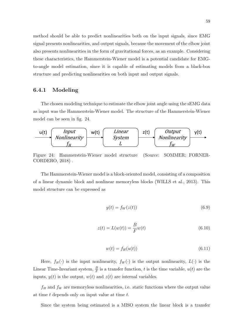
59
method should be able to predict nonlinearities both on the input signals, since EMG
signal presents nonlinearities, and output signals, because the movement of the elbow joint
also presents nonlinearities in the form of gravitational forces, as an example. Considering
these characteristics, the Hammerstein-Wiener model is a potential candidate for EMG-
to-angle model estimation, since it is capable of estimating models from a black-box
structure and predicting nonlinearities on both input and output signals.
6.4.1 Modeling
The chosen modeling technique to estimate the elbow joint angle using the sEMG data
as input was the Hammerstein-Wiener model. The structure of the Hammerstein-Wiener
model can be seen in fig. 24.
Figure 24: Hammerstein-Wiener model structure (Source: SOMMER; FORNER-CORDERO, 2018) .
The Hammerstein-Wiener model is a block-oriented model, consisting of a composition
of a linear dynamic block and nonlinear memoryless blocks (WILLS et al., 2013). This
model structure can be expressed as
y(t) = fW (z(t)) (6.9)
z(t) = L(w(t)) =B
Fw(t) (6.10)
w(t) = fH(u(t)) (6.11)
Here, fH(·) is the input nonlinearity, fW (·) is the output nonlinearity, L(·) is the
Linear Time-Invariant system, BF
is a transfer function, t is the time variable, u(t) are the
inputs, y(t) is the output, w(t) and z(t) are internal variables.
fH and fW are memoryless nonlinearities, i.e. static functions where the output value
at time t depends only on input value at time t.
Since the system being estimated is a MISO system the linear block is a transfer

60
function vector in the form
Bi(q)
Fi(q)(6.12)
Where i = 1, 2, 3 and q is the delay operator, representing the delay in time for each
input to the system.
To determine the system, the orders of the numerator nb and denominator nf of the
transfer function, as well as the input delays nk, must be specified.
In order to find a solution a hard search was done using 1000 models with random
orders ranging from 1 to 15. A window of 6s from the data vector was used to calibrate
the model, while the entire data vector was used to validate the estimated model.
The following input and output nonlinearities were tested for each model: sigmoid
network, wavelet network, piecewise linear function and one-dimensional polynomial.
Sigmoid network is a nonlinear estimator that combines a neural network with a
sigmoid as the activation function (PATCHARAPRAKITI et al., 2011). It is represented
by the equation 6.13:
y(u) = (u− r)PL+n∑i
aif((u− r)Qbi − ci) + d (6.13)
where f is the sigmoid function, given by the following equation:
f(z) =1
e−z + 1(6.14)
when u is the input; y is the output; r is the regressor; Q is a nonlinear subspace; P a
linear subspace; L is a linear coefficient; d is an output offset; b is a dilation coefficient; c
a translation coefficient and a is an output coefficient. The sigmoid network is calculated
in Matlab R© (The Mathworks Inc, USA) through the use of an iterative search technique
for estimating parameters.
Wavelet network is a feed-forward neural network using wavelet as an activation func-
tion, based on the following equation 6.15:
y(u) = (u− r)PL+n∑i
asif(bs(u− r)Q+ cs) +n∑i
awig(bwi(u− r)Q+ cwi) + d (6.15)

61
Where u is the input function; y is the output;Q is a nonlinear subspace; P is a linear
subspace; L is a linear coefficient; d is output offset; as is a scaling coefficient; aw is a
wavelet coefficient; bs is a scaling dilation coefficient; bw is a wavelet dilation coefficient; cs
is a scaling translation coefficient and cw is a wavelet translation coefficient. The scaling
function f(.) is shown in equation 6.16 and wavelet function g(.) in equation 6.17:
f(u) = exp(−0.5 ∗ u′ ∗ u) (6.16)
g(u) = (dim(u)− u′ ∗ u) ∗ exp(−0.5 ∗ u′ ∗ u) (6.17)
Its parameters are determined in Matlab R© (The Mathworks Inc, USA) by iterative
minimization.
Piecewise linear nonlinearity is a piecewise-defined function, composed of straight-line
sections (STANLEY, 2004). It is defined by the equation 6.18:
y = F (x, θ) (6.18)
Where y and x are scalars, and θ represents the parameters specifying the number of
break points and the value of nonlinearity at the break points (MATHWORKS, 2016).
One-dimensional polynomial nonlinearity uses a one-dimensional polynomial as non-
linearity. The form of this nonlinearity can be expressed as in equation 6.19:
y = F (x)F (x) = c(1)xn + c(2)x(n−1) + ...+ c(n)x+ c(n+ 1) (6.19)
Each model was compared to the reference angle using equations 6.6 and 6.7. The
model orders that achieved the highest fitness value from these equations were chosen.
The parameters of the models were estimated using time-domain data in Matlab R© (The
Mathworks Inc, USA).
The coefficient of determination R2 was also used to measure the fitness of the pro-
posed model.
R2 = 1− SSresSStot
(6.20)
Where
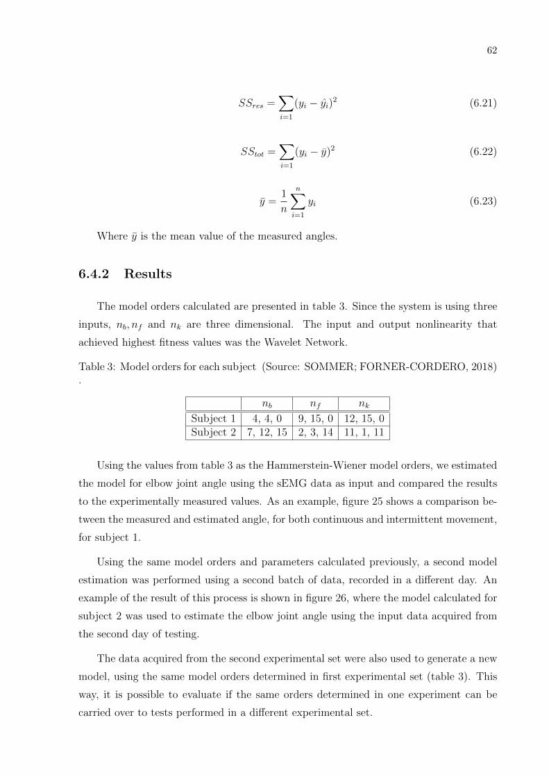
62
SSres =∑i=1
(yi − yi)2 (6.21)
SStot =∑i=1
(yi − y)2 (6.22)
y =1
n
n∑i=1
yi (6.23)
Where y is the mean value of the measured angles.
6.4.2 Results
The model orders calculated are presented in table 3. Since the system is using three
inputs, nb, nf and nk are three dimensional. The input and output nonlinearity that
achieved highest fitness values was the Wavelet Network.
Table 3: Model orders for each subject (Source: SOMMER; FORNER-CORDERO, 2018).
nb nf nk
Subject 1 4, 4, 0 9, 15, 0 12, 15, 0Subject 2 7, 12, 15 2, 3, 14 11, 1, 11
Using the values from table 3 as the Hammerstein-Wiener model orders, we estimated
the model for elbow joint angle using the sEMG data as input and compared the results
to the experimentally measured values. As an example, figure 25 shows a comparison be-
tween the measured and estimated angle, for both continuous and intermittent movement,
for subject 1.
Using the same model orders and parameters calculated previously, a second model
estimation was performed using a second batch of data, recorded in a different day. An
example of the result of this process is shown in figure 26, where the model calculated for
subject 2 was used to estimate the elbow joint angle using the input data acquired from
the second day of testing.
The data acquired from the second experimental set were also used to generate a new
model, using the same model orders determined in first experimental set (table 3). This
way, it is possible to evaluate if the same orders determined in one experiment can be
carried over to tests performed in a different experimental set.
63
Figure 25: Comparison between the measured angle of the elbow joint and the anglecalculated through the use of the estimated model, for subject 1, with a 1.5kg dumbbell.a) shows the comparison for the continuous movement and b) the comparison for theintermittent movement (Source: SOMMER; FORNER-CORDERO, 2018) .

64
Figure 26: Comparison of the estimated and measured joint angle using the same modelcalculated with the first data set, but using the EMG data from the second test set asinput for subject 2 with a 1.5kg dumbbell. a) shows the comparison for the continu-ous movement and b) the comparison for the discrete movement (Source: SOMMER;FORNER-CORDERO, 2018) .

65
To better determine the accuracy of the model, three performance parameters were
used: the correlation coefficient, the determination coefficient and the root-mean-square
Error (RMSE) between the estimated and the measured elbow joint angles. Table 4
shows the accuracy performance parameters for each participant and every test set. The
different results for each method described above are presented in columns. First, using
the first data set to estimate a model and comparing the result to the measured angle
values; second, using the same model calculated for the first experimental set to estimate
the angle, but using the data from the second experimental set as input to the model; and
finally, using the same model orders chosen from the first experimental set, a new model
was generated based on the second data set and comparing the output to the measured
angle data.
Table 4: Correlation factor, coefficient of determination and root-mean-square error forthe calculated and measured angle values (Source: SOMMER; FORNER-CORDERO,2018) .
Model Estimation, first test set Same model, second test set New model, same orders, second test setContinuous Intermittent Continuous Intermittent Continuous Intermittent
Correlation R2 RMSE Correlation R2 RMSE Correlation R2 RMSE Correlation R2 RMSE Correlation R2 RMSE Correlation R2 RMSE
0 kg 0.9623 0.9232 9.394 0.9624 0.8932 12.91 0.8780 0.5114 17.86 0.9697 0.9205 9.647 0.9525 0.9044 7.898 0.9708 0.8602 12.79Subject 1 1.5 kg 0.9780 0.9480 7.390 0.9865 0.9714 6.846 0.9129 0.7403 14.21 0.9666 0.9339 8.870 0.9169 0.8400 11.15 0.9328 0.8470 13.50
3 kg 0.9816 0.9499 6.796 0.9631 0.9200 11.477 0.9330 0.8526 10.31 0.7956 0.6161 22.70 0.9497 0.8912 8.860 0.9730 0.8923 12.030 kg 0.9729 0.9440 7.662 0.9620 0.9244 10.10 0.8825 0.7669 16.44 0.9330 0.8657 13.98 0.9787 0.9570 7.062 0.9620 0.9099 11.45
Subject 2 1.5 kg 0.9596 0.9202 8.9476 0.9493 0.8859 11.62 0.9754 0.9425 7.927 0.9413 0.8683 14.09 0.9838 0.9673 5.976 0.9211 0.8482 15.123 kg 0.9788 0.9556 6.733 0.9808 0.9612 6.540 0.8767 0.7668 15.35 0.9625 0.9191 11.02 0.9847 0.9688 5.614 0.9721 0.9431 9.246
The estimated models achieved correlation values of 94.90 ± 3.92%, coefficient of
determination of 0.8814± 0.0978 and RMSE values of 10.82± 3.73◦
6.5 Discussion and Conclusions
This chapter proposed a method for determining the elbow joint angle based on the
measurement of the sEMG of biceps brachii, triceps brachii and brachioradialis. The arm
model was estimated using the data collected from the experiment and system identifica-
tion methods. The system identification methods used were ARIMAX and Hammerstein-
Wiener model with Wavelet Network as input and output nonlinearities. With the ac-
quired sEMG data as input to the estimated model, it was possible to obtain an estimation
of the elbow joint angle. Using the data from the IMU it was possible to validate the
estimation based on sEMG.
The experimental data showed that it is possible to use the EMG data to estimate the
joint angle, with prior knowledge of the weight being lifted, at least for the experimental
conditions performed during the tests.
Both methods achieved good results in regards of the precision of angle estimation.

66
Since we are aiming at developing a real-time controller for the exoskeleton, a model with
less complexity grants more advantageous characteristics, such as fewer calibration time
and faster real-time calculation for angle estimation. For this reason, the linear model is
the model chosen for further testing in real-time conditions.
In the next part, testing of the linear model, in a real-time condition, is performed.

PART IV
TESTING

68
7 CONTROL TESTING
To test the controller, the experiment must be conducted in two steps:
1. Similar to the tests performed for linear and nonlinear model calibration in chapter
6, a calibration procedure is made, recording the signal from the muscles, while the
subject performs arm flexo-extension movements, with different weights. With this
data, it is possible to estimate a dynamic model for the EMG-to-Angle relation;
2. With the dynamic model estimated, the input signal now serves as real-time input
to the model, resulting in the corresponding angle estimation for the exoskeleton.
In the following sections, these experiments are described and the obtained results are
shown.
7.1 Calibration
7.1.1 Equipment and Materials
7.1.1.1 EMG sensor
Even though the (FREEEMG 1000, BTS Bioengineering Corp., Italy) electrodes
present high levels of accuracy, its larger dimensions and difficulty to establish com-
munication with external hardware without dedicated software presents setbacks to its
application in a real-time controller. For this reason, it is necessary to use another sensor
for the acquisition of EMG data.
The chosen device for this end was the (Muscle Sensor V3, Sparkfun Electronics R©,
USA). Its low dimensions together with its ease of communication with microprocessors
makes this device a great candidate for this specific application.
Connected to this sensor, a trio of electrodes must be connected: a pair of these
electrodes is attached to the target muscle, while the third electrode must be attached to

69
an electrically neutral portion of the body (such as a bony area), to serve as the ground
reference for the device. The pair of electrodes placed at the muscle do the acquisition of
EMG in an differential configuration, to filter noises in the EMG signal.
The device works by acquiring the signal from the electrodes; the signal is amplified
by the AD8221 differential amplifier; the signal is amplified again in two steps with two
TL084 operational amplifiers; then it is rectified by the 1N4148 diodes; the rectified signal
is filtered in a low-pass filter; the signal is amplified by an adjustable gain amplifier. The
Muscle Sensor V3 output can be connected directly to a microprocessor. An schematic of
this device can be found at the Annex section of this work.
7.1.1.2 Microprocessor
The (FREEEMG 1000, BTS Bioengineering Corp., Italy) did the recording of the
EMG data for the previous experiment. Since the (Muscle Sensor V3, Sparkfun Electronics R©,
USA) has been chosen for this new experiment, a microprocessor is required to do the
recording of the data.
The chosen microprocessor for this end is the (Arduino UNO, Arduino, S.r.l., Italy).
The Arduino Uno has low dimensions, making it portable; communication with the (Mus-
cle Sensor V3, Sparkfun Electronics R©, USA) is straightforward, requiring only the con-
nection of the output from the EMG acquisition device to one of the analog inputs in the
Arduino Uno; it has an embedded Analog-to-Digital converter; the ModExo exoskeleton
already has an Arduino, being possible to modify the current software to record the data
from the EMG acquisition device.
7.1.2 Subjects and experimental setup
One volunteer with no known neuromuscular deficit participated in the experiment.
Surface Electromyography (sEMG) of one right arm muscle, biceps brachii, was recorded.
sEMG was measured with 1 trio of electrodes connected to (Muscle Sensor V3, Sparkfun
Electronics R©, USA), that communicated with the Arduino, the latter recording the EMG
data. Electrodes were placed with a separation of 20mm with the electrode diameter being
4mm. A pair of electrodes was placed on the biceps following the SENIAM guidelines
(SENIAM, 2004). The third electrode was placed at the acromion. The sampling rate
was of 20Hz. The user interface was the Arduino Serial Monitor.
70
7.1.3 Experimental protocol
The experimental protocol is similar to the experiment performed in chapter 6, being
adapted to the new hardware setup. The subject sat on a chair, with the knees flexed at
90◦, the back perpendicular to the ground. The back of the arm was leaning against a
rubber support that was attached to the chair.
The subject was asked to perform consecutive elbow flexion and extension movements
from 50◦ to 140◦ with a frequency of 0.5Hz. To achieve the desired movement speed a
metronome was set at the speed of 60 BPM so that the subject could synchronize the
movements with the sound of the metronome. This movement was repeated with 2kg and
3kg extra weight placed at the subject’s hand.
All the data from the tests were transferred to Matlab R© for further analysis and
processing.
To reduce the complexity in processing the data and calibrating the model, the user
did not perform intermittent flexion and extension movements.
7.1.4 Experimental data processing
The signal from the Muscle Sensor V3 is already rectified. A 10-point moving average
was applied to further smooth the signal, to achieve a better result for the estimated
model.
Since the position tracking data was sampled at 100 Hz while the EMG data was
sampled at 20hz, all the position tracking data was resampled to 20 Hz.
7.1.5 Modeling
According to the results found in chapter 6, the FIR model is the linear model that
achieves the best accuracy results. For this reason, it was the chosen model for application
in the exoskeleton. In this case, the FIR model was estimated using data from the biceps
muscle alone.
In order to find a solution, a hard search was done using 1000 different random model
orders ranging from 1 to 10 for the na and nb and 0 to 4 for nk. Reduction of the nk
order has low impact in the model accuracy, while a reduction in its order reduces the
computational effort of the microprocessor. The entire data window was used to calibrate
the model, since the validation will be made through real time testing.
71
Each model was compared to the reference angle using equation 6.6. The orders of
the model that achieved the highest fitness value were chosen. The parameters of the
models were estimated using time-domain data in Matlab R©.
7.2 Testing
7.2.1 Data processing
For the testing of the controller, the same hardware configuration was used. The EMG
data was acquired by the (Muscle Sensor V3, Sparkfun Electronics R©, USA), sending the
data to the microprocessor. Data processing occurred as follows:
1. A 10-point moving average filter was applied to the EMG signal, replicating the
same filter applied in the estimation of the model;
2. To simulate the detrending of the EMG data, the mean value of the EMG data used
in the calibration procedure was subtracted in real time from the EMG signal;
3. Then, the data was used as input to the model calibrated on the previous section;
4. Since the output from the model is also a detrended value, to estimate the elbow
joint angle the mean value of the elbow joint angle (acquired in the calibration
procedure) was summed to the output of the model.
The model calculations were performed by the microprocessor.
The estimation of the joint angle can be represented as in 7.1.
A(q)θ(n) = B(q)[V (n− nk)− V ] + θ (7.1)
Where θ(n) is the output angle of the elbow joint at discrete time n; θ is the mean
value of the elbow joint angle; V (n) is the input, being the processed sEMG values from
biceps brachii; V is the mean value of the sEMG signal; nk is the delay for sEMG input;
q is the delay operator; A and B are the model parameters, defined by:
A(q) = 1 + a1q−1 + · · ·+ anaq
−na (7.2)
B(q) = 1 + b1q−1 + · · ·+ bnbq
−nb+1 (7.3)
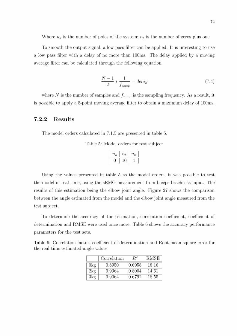
72
Where na is the number of poles of the system; nb is the number of zeros plus one.
To smooth the output signal, a low pass filter can be applied. It is interesting to use
a low pass filter with a delay of no more than 100ms. The delay applied by a moving
average filter can be calculated through the following equation
N − 1
2∗ 1
fsamp= delay (7.4)
where N is the number of samples and fsamp is the sampling frequency. As a result, it
is possible to apply a 5-point moving average filter to obtain a maximum delay of 100ms.
7.2.2 Results
The model orders calculated in 7.1.5 are presented in table 5.
Table 5: Model orders for test subject
na nb nk
0 10 4
Using the values presented in table 5 as the model orders, it was possible to test
the model in real time, using the sEMG measurement from biceps brachii as input. The
results of this estimation being the elbow joint angle. Figure 27 shows the comparison
between the angle estimated from the model and the elbow joint angle measured from the
test subject.
To determine the accuracy of the estimation, correlation coefficient, coefficient of
determination and RMSE were used once more. Table 6 shows the accuracy performance
parameters for the test sets.
Table 6: Correlation factor, coefficient of determination and Root-mean-square error forthe real time estimated angle values
Correlation R2 RMSE
0kg 0.8950 0.6958 18.162kg 0.9364 0.8004 14.613kg 0.9064 0.6792 18.55

73
Figure 27: Comparison between the measured angle of the elbow joint and the anglecalculated through the model in real time. a) shows the comparison for no extra weightb) the comparison for 2kg extra weight and c) the comparison for 3kg extra weight

74
7.3 Discussion and Conclusions
This chapter proposed a method and presented an experiment on the feasibility of real
time exoskeleton control, using a linear model estimated through system identification.
The system model was estimated using data collected from the experiment and a linear
system identification method. With the model estimated, EMG data from biceps brachii
was used as real time input for the model. As so, the output angle of the exoskeleton
could be calculated.
The experimental data showed that the real time application of the EMG-driven
controller was successful. Even though the results showed slightly inferior performance
values to the offline testing, they are still deemed good compared to similar works already
developed and referenced in this work.
The results of this testing have been accepted for publication in the conference IEEE
EMBC 2019 (SUPLINO; SOMMER; FORNER-CORDERO, 2019).

PART V
DISCUSSIONS, CONCLUSIONS AND FUTURE
WORK

76
8 DISCUSSIONS AND CONCLUSIONS
This work presented the design of an EMG-driven exoskeleton controller. Biomecha-
tronics was combined with control design and system modeling to achieve the design of a
controller that determines the intended movement and joint angle based on sEMG of the
user’s muscles.
Three different exoskeleton platforms, each with its own characteristics, were analyzed
to determine which one better suited the application of the controller designed is this work.
The exoskeleton platforms analyzed were the ETMICAE, ULEXO and ModExo. Built
as an experimental workbench, the ModExo presents many advantages over the other
exoskeletons, such as: embedded position and force sensors; easy-to-use communication
between the platform, a computer and microprocessors; and robust and stable structure.
For these reasons, the ModExo was the exoskeleton platform which better fitted the goals
of this work. The main drawback of this option was the low computing capacities of its
microprocessor.
Experimental procedures were conducted with six volunteers subjects to obtain EMG
and angle data for the controller design. EMG from three arm muscles and elbow joint
angle data were recorded in a controlled environment, where the test subjects were asked
to perform continuous and intermittent elbow flexion and extensions, under three loading
conditions: no load, 1.5kg and 3kg weights on the hand. The experiments were conducted
in two different days for each subject. A total of 72 experimental sets were recorded. Data
acquired through these experiments were used for system identification of the EMG-to-
Angle relation.
Two different EMG-to-Angle model identification methods were proposed: one linear
and the other nonlinear. For the linear method, four different modeling techniques were
applied to determine which one best estimated the model. The modeling techniques were:
ARX, ARMAX, ARIMAX and SS. The FIR model, a particular form of the ARX model,
outperformed the other models and was the chosen modeling technique for linear system
identification.
77
For the nonlinear method, the Hammerstein-Wiener model was chosen due to its
capacity of estimating models from a black-box structure and predicting nonlinearities on
both input and output signals.
Results for the linear model show similar precision values to those achieved by other
authors (PANG et al., 2015; LIU; HERZOG; SAVELBERG, 1999; RAHMATIAN; MAHJOOB;
HANACHI, 2016; MAMIKOGLU et al., 2016). For most of the simulations, the model
achieved correlations above 90% and RMSE under 20◦. Considering the worse results, the
correlation was above 70% and the RMSE lower than 25◦.
In most of the subjects, it was not possible to use the same model to estimate the
elbow joint angle for tests conducted in different days. One way to address this problem
would be to rescale the output signal to the angle range, minimizing the RMSE of the
output signal. Since the EMG signals may change for one session to another, due to
several reasons as slight change in electrode position, tissue properties or temperature
(SODERBERG et al., 1975), it may not be possible to determine a model that estimates
the joint angle for data acquired on different days or test setups, using the methods
described in this work. Keeping this in mind, a solution would be to recalibrate the
model at each session.
For subjects 2 and 3, using the same model for experimental data from two different
days achieved correlation above 75% and RMSE below 32◦. For subject 3, specifically,
using the same model achieved values of correlation above 90% and RMSE below 20◦.
However, it is possible to note that the estimation is not as precise as it was when using
the model identification data set as input, these results can be regarded as very good
compared to other similar works. More investigation is required to determine if those
models are capable of estimating the joint angle for any test conducted with these subjects.
The same model order calculated in the first test can be used for the subsequent test
sessions, without a reduction in the accuracy of the predicted angle. This shows that,
even considering that environmental noise affects the EMG signal, it does not change the
system order. With the model orders already calculated, a recalibration procedure can
be quickly applied, minimizing the problem of model non-repeatability.
For the nonlinear model, it achieved better results compared to the linear model. Even
though other authors used the Hammerstein-Wiener model to determine EMG-to-Muscle
Force relation instead of a EMG-to-Angle relation, the results show similar precision
values (ABBASI-ASL et al., 2011; SEBASTIAN et al., 2010; CLANCY et al., 2012).
In most of the simulations, the model achieved values of correlation over 90%, coef-

78
ficient of determination over 0.9 and RMSE under 15◦. For both subjects, in the worst
case, correlation was above 79%, coefficient of determination above 0.5 and RMSE below
23◦ when compared to the measured elbow joint angles.
As with the linear model, simulation results when using the same model for different
data inputs are worse than the results presented when using the same data used for model
calibration. But in this case, these results can be favorably compared to other similar
works. Also, as before, the same model orders calculated through the first experimental
set can be used for other test sessions, without loss of accuracy.
Linear system identification method was chosen and adapted for real time experi-
ments. It was chosen over the nonlinear method since it could be better adapted to the
available hardware and required less computational power. As such, the system identi-
fication method was adapted and implemented to function with a microprocessor and a
different EMG acquisition equipment. A new experiment was conducted to calibrate a
model using the new hardware.
With the linear model calibrated, testing of the controller in real time was performed.
The test subject was asked to perform the same consecutive and continuous elbow flexion
and extension performed in previous testing, with no extra weight, 2kg and 3kg extra
weight. The results prove that the real time application of the EMG-driven exoskeleton
control is possible in the proposed environment.
The real time controller achieved values of correlation, coefficient of determination
and RMSE of 91.26% ± 2.14%, 0.7251 ± 0.0657 and 17.11◦ ± 2.17◦, respectively. In the
worst results, correlation was over 89%, coefficient of determination over 0.67 and RMSE
under 20◦. Care must be taken when inferring the applicability of this model to other
test subjects. But as a proof of concept, the controller was successful in estimating the
elbow joint angle in real time conditions.
In the end, the controller was capable of estimating the elbow joint angle using only
EMG data as input, as long as the model was calibrated to the previously known load
being carried by the user.
When referring to indirect results from this work, a database acquired from six test
subjects, totaling 72 test sets of EMG and joint angle data, has been acquired. Even
though this database has only been used for system identification modeling in this work,
its data can be further used and analyzed under a multitude of different techniques, such
as the Time Domain/Frequency Domain feature set, Neural Networks and mathematical
morphological models (e.g. Hill’s muscle model), to name a few.
79
9 FUTURE WORK
Much can be done to further improve the work presented in this dissertation. Some
of the opportunities for improvement are described in the following section:
More extensive testing and acquisition of EMG and joint angle can be done, exploring
more complex movements and replicating movements done on a daily basis. A longer
acquisition time could also benefit models that require longer training periods, which
is the case for some Neural Networks. For this end, a more portable hardware will be
required, one that is capable of measuring EMG and angle data for long periods (days,
even) with minimal negative impact on daily activities. This can further increase the
accuracy of the model, as well as serving as data for models capable of performing more
complex activities and movements.
Studying the possibility of estimating one single model for each subject, independent
of the load applied to arm/exoskeleton, can result in an even better controller. One way
to achieve this result would be to use a force sensor on the exoskeleton that measures
the load applied. According to the readings of the sensor, a state machine could make a
transition to the model corresponding to the applied load.
Hammerstein-Wiener models presented better results than the Linear system iden-
tification method. Application of the Hammerstein-Wiener model for real time testing
could present better results than the ones obtained using the linear model. Exploration
of different modeling techniques, such as Neural Networks, and the pairing with other
extensively used morphological mathematical models, such as Hill’s muscle models, can
present even better models for the EMG-to-Angle relation.
More powerful hardware for real time testing could improve both the model accuracy
as well as the output angle. Even though the Sparkfun Muscle Sensor V3 presented
good results, the quality of signal acquisition is far from other equipment, like the BTS
(FREEEMG 1000, BTS Bioengineering Corp., Italy). An EMG acquisition device that
is both portable and accurate would be the ideal hardware for this application. Also, a

80
wireless communication between the electrodes and the processing unit would also present
more freedom of movement for the user.
A subject-independent model, that can estimate joint angles for a large group of
subjects, would present a huge improvement by being able to skip the model calibration
procedure necessary between each test session.
ModExo was well suited as a platform for testing and studying the proposed methods.
But it has little to no application for movement assistance in real life activities. The
ideal scenario would be to apply the controller proposed in this work in an exoskeleton
designed for movement assistance in daily activities. When the work on the construction
of ETMICAE is finished, it can prove to be a great platform for further testing of the
proposed controller.
Above all, this work is a product of collaborative effort between many people, from
colleagues and professors at Escola Politecnica - USP to many theorists and specialists in
engineering and medicine. And it is through this collaborative effort that this work will
achieve even higher standards. As many have contributed to this work, I hope this work
will serve as contribution for many others to come.

81
REFERENCES
ABBASI-ASL, R. et al. Estimation of muscle force with emg signals using hammerstein-wiener model. In: OSMAN, N. A. A. et al. (Ed.). 5th Kuala Lumpur InternationalConference on Biomedical Engineering 2011. Berlin, Heidelberg: Springer BerlinHeidelberg, 2011. p. 157–160. ISBN 978-3-642-21729-6.
AL-TIMEMY, A. H. et al. A preliminary investigation of the effect of force variation formyoelectric control of hand prosthesis. In: 2013 35th Annual International Conferenceof the IEEE Engineering in Medicine and Biology Society (EMBC). [S.l.: s.n.], 2013. p.5758–5761. ISSN 1094-687X.
ALTER, R. Bioelectric control of prostheses. [S.l.], 1966.
AMUNDSON, K. et al. Development of hybrid hydraulic-electric power units for fieldand service robots. Advanced Robotics, v. 20, p. 1015–1034, 2006.
ANAM, K.; AL-JUMAILY, A. A. Active exoskeleton control systems: State of the art.Procedia Engineering, v. 41, p. 988 – 994, 2012. ISSN 1877-7058.
AUNG, Y.; AL-JUMAILY, A. Estimation of upper limb joint angle using surface emgsignal. International Journal of Advanced Robotic Systems, v. 10, 2013.
AZAB, A. M.; ARVANCH, M.; MIHAYLOVA, L. S. Estimation of joint angle based onsurface electromyogram signals recorded at different load levels. In: 2017 39th AnnualInternational Conference of the IEEE Engineering in Medicine and Biology Society(EMBC). [S.l.: s.n.], 2017. p. 2538–2541. ISSN 1557-170X.
BATTYE, C. K.; NIGHTINGALE, A.; WHILLIS, J. The use of myo-electric currents inthe operation of prostheses. Bone & Joint Journal, Bone and Joint Journal, v. 37-B,n. 3, p. 506–510, 1955. ISSN 0301-620X.
BOTTOMLEY, A. H. Myo-electric control of powered prostheses. Bone & Joint Journal,Bone and Joint Journal, v. 47-B, n. 3, p. 411–415, 1965. ISSN 0301-620X.
CHEN, X.; CHEN, S.; DAN, G. Control of powered prosthetic hand usingmultidimensional ultrasound signals: A pilot study. In: STEPHANIDIS, C. (Ed.).Universal Access in Human-Computer Interaction. Applications and Services: 6thInternational Conference, UAHCI 2011, Held as Part of HCI International 2011,Orlando, FL, USA, July 9-14, 2011, Proceedings, Part IV. Berlin, Heidelberg: SpringerBerlin Heidelberg, 2011. p. 322–327. ISBN 978-3-642-21657-2.
CHILDRESS, D. S.; HOLMES, D. W.; BILLOCK, J. N. Ideas on myoelectric prostheticsystems for upper-extremity amputees. The Control of Upper-extremity Prostheses andOrthoses, Charles C. Thomas, p. 86–106, 1971.

82
CHU, A.; KAZEROONI, H.; ZOSS, A. On the biomimetic design of the berkeleylower extremity exoskeleton (bleex). In: Proceedings of the 2005 IEEE InternationalConference on Robotics and Automation. [S.l.: s.n.], 2005. p. 4345–4352. ISSN 1050-4729.
CLANCY, E. A. et al. Identification of constant-posture emg-torque relationshipabout the elbow using nonlinear dynamic models. IEEE Transactions on BiomedicalEngineering, v. 59, n. 1, p. 205–212, Jan 2012. ISSN 0018-9294.
CYBERDYNE. Cyberdine Products, Available in : https://www.cyberdyne.jp/english/.Access in 16/06/2017. 2007.
DOLLAR, A. M.; HERR, H. Lower extremity exoskeletons and active orthoses:Challenges and state-of-the-art. IEEE Transactions on Robotics, v. 24, n. 1, p. 144–158,Feb 2008. ISSN 1552-3098.
ENGLEHART, K.; HUDGINS, B. A robust, real-time control scheme for multifunctionmyoelectric control. IEEE Transactions on Biomedical Engineering, v. 50, n. 7, p.848–854, July 2003. ISSN 0018-9294.
ENGLEHART, K. et al. Classification of the myoelectric signal using time-frequencybased representations. Medical Engineering & Physics, v. 21, n. 6–7, p. 431 – 438, 1999.ISSN 1350-4533.
ESQUENAZI, A. New bipedal locomotion option for individuals with thoracic levelmotor complete spinal cord injury. J. Spinal Res. Found., v. 8, p. 26–28, 2013.
EVANS, H. B. et al. Signal processing for proportional myoelectric control. IEEETransactions on Biomedical Engineering, BME-31, n. 2, p. 207–211, Feb 1984. ISSN0018-9294.
FARINA, D.; MERLETTI, R.; ENOKA, R. M. The extraction of neural strategies fromthe surface emg: an update. Journal of Applied Physiology, American PhysiologicalSociety, v. 117, n. 11, p. 1215–1230, 2014. ISSN 8750-7587.
FINEBERG, D. B. et al. Vertical ground reaction force-based analysis of poweredexoskeleton-assisted walking in persons with motor-complete paraplegia. The Journal ofSpinal Cord Medicine, v. 36(4), p. 313–321, 2013.
FOUGNER, A. et al. Cancellation of force induced artifacts in surface emg using fsrmeasurements. Proc. Myoelectric Controls Symp. (MEC), 2008.
FOUGNER, A. et al. Resolving the limb position effect in myoelectric patternrecognition. IEEE Transactions on Neural Systems and Rehabilitation Engineering,v. 19, n. 6, p. 644–651, Dec 2011. ISSN 1534-4320.
FRANCESCHINI, M. et al. Reciprocating gait orthoses: A multicenter study of theiruse by spinal cord injured patients. Archives of Physical Medicine and Rehabilitation,v. 78, n. 6, p. 582 – 586, 1997. ISSN 0003-9993.
GARCIA, E.; SATER, J. M.; MAIN, J. Exoskeletons for human performanceaugmentation (ehpa) : A program summary. Journal of the Robotics Society of Japan,v. 20, n. 8, p. 822–826, 2002.

83
GHAN, J.; KAZEROONI, H. System identification for the berkeley lower extremityexoskeleton (bleex). In: Proceedings 2006 IEEE International Conference on Roboticsand Automation, 2006. ICRA 2006. [S.l.: s.n.], 2006. p. 3477–3484. ISSN 1050-4729.
HAYASHIBE, M.; GUIRAUD, D.; POIGNET, P. EMG-to-force estimation withfull-scale physiology based muscle model. In: IROS’09: International Conference onIntelligent Robots and Systems. St. Louis, MO, United States: IEEE/RSJ, 2009. p.1621–1626.
HOGAN, N.; MANN, R. W. Myoelectric signal processing: Optimal estimation appliedto electromyography - part i: Derivation of the optimal myoprocessor. IEEE Transactionson Biomedical Engineering, BME-27, n. 7, p. 382–395, July 1980. ISSN 0018-9294.
HOGAN, N.; MANN, R. W. Myoelectric signal processing: Optimal estimation appliedto electromyography - part ii: Experimental demonstration of optimal myoprocessorperformance. IEEE Transactions on Biomedical Engineering, BME-27, n. 7, p. 396–410,July 1980. ISSN 0018-9294.
HUDGINS, B.; PARKER, P.; SCOTT, R. N. A new strategy for multifunctionmyoelectric control. IEEE Transactions on Biomedical Engineering, v. 40, n. 1, p. 82–94,Jan 1993. ISSN 0018-9294.
IBGE. Censo demografico 2010 - caracterısticas gerais da populacao, religiao e pessoascom deficiencia. IBGE, Rio de Janeiro, Brazil, 2012.
ISIDORI, A.; NICOLO, F. A device for the detection and measurement of someparameters of myoelectric potentials. Report no. 11, Electrotechnical Institute, Universityof Rome, Electrotechnical Institute, University of Rome, 1966.
JIANG, N.; ENGLEHART, K. B.; PARKER, P. A. Extracting simultaneous andproportional neural control information for multiple-dof prostheses from the surfaceelectromyographic signal. IEEE Transactions on Biomedical Engineering, v. 56, n. 4, p.1070–1080, April 2009. ISSN 0018-9294.
KATO, A. et al. Estimating a joint angle by means of muscle bulge movement alonglongitudinal direction of the forearm. In: 2015 IEEE International Conference onRobotics and Biomimetics (ROBIO). [S.l.: s.n.], 2015. p. 614–619.
KAWAMOTO, H. et al. Voluntary motion support control of robot suit hal triggered bybioelectrical signal for hemiplegia. In: 2010 Annual International Conference of the IEEEEngineering in Medicine and Biology. [S.l.: s.n.], 2010. p. 462–466. ISSN 1094-687X.
KAZEROONI, H. The berkeley lower extremity exoskeleton. In: . Field andService Robotics: Results of the 5th International Conference. Berlin, Heidelberg:Springer Berlin Heidelberg, 2006. p. 9–15. ISBN 978-3-540-33453-8.
KENNEY, L. et al. Dimensional change in muscle as a control signal for powered upperlimb prostheses: a pilot study. Medical Engineering & Physics, v. 21, n. 8, p. 589–597,1999. ISSN 1350-4533.
LENZI, T. et al. Intention-based emg control for powered exoskeletons. IEEETransactions on Biomedical Engineering, v. 59, n. 8, p. 2180–2190, Aug 2012. ISSN0018-9294.

84
LIU, M.; HERZOG, W.; SAVELBERG, H. Dynamic muscle force predictions from emg:An artificial neural network approach. Journal of Electromyography and Kinesiology,v. 9, n. 6, p. 391–400, 1999.
LOSIER, Y.; ENGLEHART, K.; HUDGINS, B. A control system for a poweredprosthesis using positional and myoelectric inputs from the shoulder complex. In: 200729th Annual International Conference of the IEEE Engineering in Medicine and BiologySociety. [S.l.: s.n.], 2007. p. 6137–6140. ISSN 1094-687X.
MACKAY, J. et al. The Atlas of Heart Disease and Stroke. [S.l.]: World HealthOrganization, 2004. (Academic Search Complete). ISBN 9789241562768.
MAMIKOGLU, U. et al. Elbow joint angle estimation by using integrated surfaceelectromyography. In: . [S.l.: s.n.], 2016. p. 785–790.
MATHWORKS. armax. Available in:https://www.mathworks.com/help/ident/ref/armax.html. Access in 06/07/2019.2015.
MATHWORKS. pwlinear. Available in:https://www.mathworks.com/help/ident/ref/pwlinear.html. Access in 06/07/2019.2016.
MERRIAMWEBSTERDICTIONARY. Biomimetics definition. Available in:https://www.merriam-webster.com/dictionary/biomimetics. Access in 11/07/2017. 2009.
MIRANDA, A. B. W.; FORNER-CORDERO, A. Upper limb exoskeleton control basedon sliding mode control and feedback linearization. In: 2013 ISSNIP Biosignals andBiorobotics Conference: Biosignals and Robotics for Better and Safer Living (BRC).[S.l.: s.n.], 2013. p. 1–6. ISSN 2326-7844.
NIELSEN, J. L. G. et al. Enhanced emg signal processing for simultaneous andproportional myoelectric control. In: 2009 Annual International Conference of the IEEEEngineering in Medicine and Biology Society. [S.l.: s.n.], 2009. p. 4335–4338. ISSN1094-687X.
NIGHTINGALE, J. Microprocessor control of an artificial arm. Journal of MicrocomputerApplications, v. 8, n. 2, p. 167 – 173, 1985. ISSN 0745-7138.
OTSUKA, T. et al. Development of upper-limb type hal and reaching movement formeal-assistance. In: 2011 IEEE International Conference on Robotics and Biomimetics.[S.l.: s.n.], 2011. p. 883–888.
PANG, M. et al. Electromyography-based quantitative representation method forupper-limb elbow joint angle in sagittal plane. Journal of Medical and BiologicalEngineering, v. 35, n. 2, p. 165–177, 2015.
PARKER, P.; STULLER, J.; SCOTT, R. Signal processing for the multistate myoelectricchannel. Proceedings of the IEEE, v. 65, n. 5, p. 662–674, 1977.
PATCHARAPRAKITI, N. et al. Modeling of photovoltaic grid connected inverters basedon nonlinear system identification for power quality analysis. 2011.

85
PHILIPSON, L. Adaptable myoelectric prosthetic control with functional visual feedbackusing microprocessor techniques. Medical and Biological Engineering and Computing,v. 23, n. 1, p. 8–14, 1985. ISSN 1741-0444.
PONS, J. Wearable Robots: Biomechatronic Exoskeletons. [S.l.]: Wiley, 2008. ISBN9780470987650.
RAHMATIAN, S.; MAHJOOB, M.; HANACHI, M. Continuous estimation of ankle jointangular position based on the myoelectric signals. In: . [S.l.: s.n.], 2016. p. 158–163.
ROSE, W. Electromyogram Analysis. Available in:https://www1.udel.edu/biology/rosewc/kaap686/notes/EMG%20analysis.pdf. Ac-cess in 12/11/2016. 2011.
SANKAI, Y. Hal: Hybrid assistive limb based on cybernics. In: . RoboticsResearch: The 13th International Symposium ISRR. Berlin, Heidelberg: Springer BerlinHeidelberg, 2011. p. 25–34. ISBN 978-3-642-14743-2.
SEBASTIAN, A. et al. Analysis of emg-force relation using system identification andhammerstein-wiener models. ASME 2010 Dynamic Systems and Control Conference,v. 1, p. 381–388, Jan 2010. ISSN 0018-9294.
SENIAM. Recommendations for sensor locations in arm or hand muscles., Available in :http://seniam.org/. Access in 10/11/2016. 2004.
SILVA, J.; CHAU, T.; GOLDENBERG, A. Mmg-based multisensor data fusion forprosthesis control. In: Proceedings of the 25th Annual International Conference of theIEEE Engineering in Medicine and Biology Society (IEEE Cat. No.03CH37439). [S.l.:s.n.], 2003. v. 3, p. 2909–2912 Vol.3. ISSN 1094-687X.
SLOTINE, J.-J. E.; LI, W. Applied nonlinear control. Upper Saddle River, NJ: Pearson,1991.
SODERBERG, G. et al. Selected Topics in Surface Electromyography for Use in theOccupational Setting: Expert Perspectives. [S.l.]: U.S. Dept. of Health and HumanServices, Public Health Service, CDC, National Institute for Occupational Safety andHealth, 1975. (DHHS publication).
SOMMER, L. F. Upper limb exoskeleton with one degree of freedom. UndergraduateThesis, Dept. Mechatronic Eng. and Mech. Systems, Escola Politecnica, University ofSao Paulo, 2015.
SOMMER, L. F. et al. Elbow joint angle estimation with surface electromyographyusing autoregressive models. In: 2018 40th Annual International Conference of the IEEEEngineering in Medicine and Biology Society (EMBC). [S.l.: s.n.], 2018. p. 1472–1475.ISSN 1558-4615.
SOMMER, L. F.; FORNER-CORDERO, A. Elbow joint angle estimation from surfaceelectromyography using hammerstein-wiener models. In: 2018 7th IEEE InternationalConference on Biomedical Robotics and Biomechatronics (Biorob). [S.l.: s.n.], 2018. p.1044–1049. ISSN 2155-1782.

86
SOUIT, C. Design and prototyping of a development platform for exoskeleton research.Master’s Dissertation, Dept. Mechatronic Eng. and Mech. Systems, Escola Politecnica,University of Sao Paulo, 2016.
SOUZA, R. S. Design and prototyping of a development platform for exoskeletonresearch. Master’s Dissertation, Dept. Mechatronic Eng. and Mech. Systems, EscolaPolitecnica, University of Sao Paulo, 2018.
STANLEY, W. D. Technical Analysis And Applications With Matlab. [S.l.]: CengageLearning, 2004. 143 p. ISBN 9781401864811.
STAVDAHL, O.; GRONNINGSAETER, A.; E.MALVIG, K. Ultrasound based estimationof muscle contraction. Dept, of Engineering Cybernetics, Norwegian University of Scienceand Technology,, 1997.
STAVDAHL, O. et al. Multimodal input device with smeg and contact force sensors.Proc. Myoelectric Controls Symp. (MEC), 2011.
STEGER, R.; KIM, S. H.; KAZEROONI, H. Control scheme and networked controlarchitecture for the berkeley lower extremity exoskeleton (bleex). In: Proceedings 2006IEEE International Conference on Robotics and Automation, 2006. ICRA 2006. [S.l.:s.n.], 2006. p. 3469–3476. ISSN 1050-4729.
SUPLINO, L. O.; SOMMER, L. F.; FORNER-CORDERO, A. Emg-based control in atest platform for exoskeleton with one degree of freedom. 2019.
TALATY, M.; ESQUENAZI, A.; BRICENO, J. E. Differentiating ability in users of therewalkTM powered exoskeleton: An analysis of walking kinematics. In: 2013 IEEE 13thInternational Conference on Rehabilitation Robotics (ICORR). [S.l.: s.n.], 2013. p. 1–5.ISSN 1945-7898.
TSUKAHARA, A. et al. Restoration of gait for spinal cord injury patients using hal withintention estimator for preferable swing speed. IEEE Transactions on Neural Systemsand Rehabilitation Engineering, v. 23, n. 2, p. 308–318, March 2015. ISSN 1534-4320.
VALIENTE, A. Design of a quasi-passive parallel leg exoskeleton to augment loadcarrying for walking. Master’s Thesis, Dept. Mech. Eng., Massachusetts Inst. Technol.,Cambridge, August, 2005.
VONSCHRADER, S.; LEE, G. Disability statistics from the current population survey(cps). Cornell University Yang Tan Institute (YTI), 2017.
WALSH, C. J. Biomimetic design of an under-actuated leg exoskeleton for load-carryingaugmentation. Master’s Thesis, Dept. Mech. Eng., Massachusetts Inst. Technol.,Cambridge, February, 2006.
WALSH, C. J.; ENDO, K.; HERR, H. A quasi-passive leg exoskeleton for load-carryingaugmentation. International Journal of Humanoid Robotics, v. 4, n. 3, p. 487–506, 2007.
WATKINS, K. Human development report 2005. American Physiological Society, 2005.
WILLS, A. et al. Identification of hammerstein–wiener models. Automatica, v. 49, n. 1,p. 70 – 81, 2013. ISSN 0005-1098.

87
YOUNG, A. J.; FERRIS, D. P. State of the art and future directions for lowerlimb robotic exoskeletons. IEEE Transactions on Neural Systems and RehabilitationEngineering, v. 25, n. 2, p. 171–182, Feb 2017. ISSN 1534-4320.
ZEILIG, G. et al. Safety and tolerance of the rewalk exoskeleton suit for ambulation bypeople with complete spinal cord injury: a pilot study. J Spinal Cord Med., v. 35(2), p.96–101, 2012.
ZOSS, A.; KAZEROONI, H. Design of an electrically actuated lower extremityexoskeleton. Advanced Robotics, v. 20, n. 9, p. 967–988, 2006.
ZOSS, A. B.; KAZEROONI, H.; CHU, A. Biomechanical design of the berkeley lowerextremity exoskeleton (bleex). IEEE/ASME Transactions on Mechatronics, v. 11, n. 2,p. 128–138, April 2006. ISSN 1083-4435.
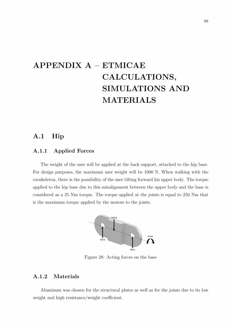
88
APPENDIX A – ETMICAE
CALCULATIONS,
SIMULATIONS AND
MATERIALS
A.1 Hip
A.1.1 Applied Forces
The weight of the user will be applied at the back support, attached to the hip base.
For design purposes, the maximum user weight will be 1000 N. When walking with the
exoskeleton, there is the possibility of the user tilting forward his upper body. The torque
applied to the hip base due to this misalignment between the upper body and the base is
considered as a 25 Nm torque. The torque applied at the joints is equal to 250 Nm that
is the maximum torque applied by the motors to the joints.
Figure 28: Acting forces on the base
A.1.2 Materials
Aluminum was chosen for the structural plates as well as for the joints due to its low
weight and high resistance/weight coefficient.

89
The shafts will be constituted of steel, since they will support high loads. Because of
its low dimensions, it is not critical the usage of low weight materials.
For the coupling of the shafts, ball bearings will be used so that the joints can rotate
with low friction coefficient, as well as being capable of enduring the high loads applied.
The chosen ball bearings were DIN 652 SKF with 2 RS1.
To avoid interference between the two parts of the joints, a Permaglide R© thrust washer
model PAW 26 will be used. This thrust washer has the necessary resistance to withstand
the applied loads. Also, it is low weight and easier to assemble compared to axial bearings.
The cover attached to the shaft will be made of aluminum.
A.1.3 Calculations and simulations
Permaglide R© PAW 26 Thrust Washer:
Torque at the hip due to the misalignment between the upper body and the rotation
axis of the hip is considered as a 25 Nm torque. This torque will be supported by the
thrust washer. That way:
M = 2 · F ·De2
+ Di2
2(A.1)
A =π4(D2
e −D2i )
2(A.2)
σ =F
A(A.3)
Figure 29: Acting forces on the abduction/adduction joint

90
Figure 30: Acting forces on the flexion/extension joint
Where M is the torque applied to the hip, F is the reaction force in the thrust washer
and cover of the joint, De and Di are the external and internal diameter of the thrust
washer, respectively, A is the thrust washer area that will support the load and σ is the
load.
Resulting in:
σ ∼= 1.5MPa < σcrit
Therefore, the PAW 26 thrust washer is suitable to be used.
DIN 625 SKF with 2 RS1 (SKF 61902-2RS1) ball bearing:
Chosen through the SKFTM bearing selection tool, for a load equal to 500 N and
lifespan of 10000 hours. The tool can be found at: http://www.skf.com/group/knowledge-
centre/engineering-tools/skfbearingselect.html
All components were numerically simulated at the AutodeskTM Inventor 2017 soft-
ware.
A.2 Knee
A.2.1 Applied forces
The forces applied at the knee joint are the torque that the motor applies at the joint
and the weight of the user and exoskeleton.

91
Figure 31: Numerical simulation of the base
Figure 32: Numerical simulation of the joint shafts

92
Figure 33: Numerical simulation of the cover
Figure 34: Forces applied to the knee joint

93
A.2.2 Materials
Aluminum is the metal constituting the joints. This material was chosen for its low
weight and high resistance/weight coefficient.
For the bars, steel bars will be used for its high resistance and easy acquisition.
For the same reasons stated at the hip, the shafts will be made of steel.
Like before, DIN 625 SKF with 2 RS1 ball bearings and PAW 26 Permaglide R© thrust
washers will be used.
A.2.3 Calculations and simulations
Figure 35: Numerical simulation of the knee joint

94
APPENDIX B – ACTUATOR CONTROL
Human limb and exoskeleton mechanics are complex and nonlinear. To account for
this complexity, it is necessary to model the interaction between exoskeleton and the
human limb when exposed to an external load.
In this annex, a study of two control methods for the actuation of the exoskeleton is
conducted: impedance control and sliding mode control.
B.1 Exoskeleton Model
B.1.1 Exoskeleton
In order to present this controller, we will use the upper limb exoskeleton described
in chapter 4. It has one degree of freedom on the elbow joint, actuated by a 12V DC
motor (578VA, Mabuchi Motor Co., ltd., Japan) with a Power Window Lifter gear trans-
mission. The transmission has a 10:1 reduction ratio. The structure of the exoskeleton is
constructed on aluminum.
The exoskeleton is illustrated in figure 36. When the user tries to flex his arm, an
electrical voltage is acquired by electrodes placed on the skin on the biceps brachii. The
(Muscle Sensor V3, Sparkfun Electronics R©, USA), was used to measure the EMG. It does
the biceps muscle voltage recording, rectification, low-pass filtering and amplification.
This signal is sent to a microprocessor (ATmega328P, Microchip Technology Inc., USA),
that makes the analog-to-digital conversion and applies a moving average filter. Finally
the voltage signal is transformed into a desired joint angle. Equation B.1 shows the
equation that gives the desired joint angle as a function of the EMG sensor voltage. A
linear relationship between the angular position and the measured voltage was chosen.
The equation was defined by measuring the EMG signal when the arm was fully extended
and when the arm was on a flexed position and linearly scaling it to the minimum angle
of 0 and maximum angle of π2. It is important to note that the voltage from the EMG

95
sensor is never zero. Even at a relaxed position, the sensor measures a residual voltage
level of -0.29V.
θd = −0.29 + 0.582 ∗ Vemg (B.1)
Figure 36: Diagram showing the exoskeleton block diagram control
With the desired joint angle the pulse-width modulation (PWM) magnitude sent to
the motor driver is calculated with a control logic in order to control the motor that
actuates the exoskeleton. This control logic will be further studied in the next section.
The motor driver input is the PWM voltage (V) and its output is an electrical current
(I). Equation B.2 shows the relationship between PWM voltage and motor current:
I = Kv ∗ V (B.2)
where Kv = 1.42 is the driver gain, V is the voltage applied to the driver and I is the
output current of the driver.
The output electrical current from the driver goes to the motor, actuating in the
exoskeleton and consequently moving the user’s forearm.
B.1.2 Modeling
Even though the exoskeleton has only one degree of freedom on the elbow joint, the
shoulder angle should also be considered because it influences the forces applied to the

96
exoskeleton and the arm. The exoskeleton can be modeled as two segments: the upper
arm (between shoulder and elbow) and the forearm (between elbow and wrist).
Figure 37: Free body diagram of the exoskeleton
Figure 37 shows the exoskeleton free body diagram, where the upper arm is considered
to be fixed at a given angle θ1. The angle between the upper arm and the forearm is θ2
with a motion range between 0 and π2
rad, the torque applied by the motor is τ , the Load
has a range between 0 and 100N, always perpendicular to exoskeleton forearm segment,
the sum of the human forearm and exoskeleton forearm masses M is equal to 2.14 kg, the
distance between the elbow center and the forearm center of mass L1 is 0.12m, the length
of the forearm L2 is 0.22m, the forearm moment of inertia Je is equal to 5.6 · 10−3kg ·m2.
Table 7: Exoskeleton model parameters
Parameter Value
Load 0 to 100NL1 0.12mL2 0.22mJe 5.6 · 10−3kg ·m2
Jm 6 · 10−5kg ·m2
B 1.2732n 10Km 0.533
Equation B.3 shows the dynamics of the exoskeleton:
(Jen
+ Jm
)· θm +B · θm = τ +
−L2 · Load− L1 ·M · g · sin(θmn
+ θ1)
n(B.3)
Where θm is the angle of the motor shaft, Jm = 6 · 10−5kg ·m2 is the motor moment
of inertia, B = 1.2732 is the damping coefficient of the motor, n = 10 is the reduction
factor and Km = 0.533 is the electrical current gain of the motor.

97
Equation B.4 gives the relation between motor input current and output torque:
τ = Km · I (B.4)
Using equations B.2, B.3 and B.4 gives the exoskeleton and human dynamics, without
considering human actuation:
(Jen
+ Jm
)· θm +B · θm = Km ·Kv · V +
−L2 · Load− L1 ·M · g · sin(θmn
+ θ1)
n(B.5)
B.2 Control
B.2.1 General Characteristics
The action control will be the voltage V applied to the driver of the motor. The load
applied to the exoskeleton can vary from 0N to 100N. In this way the user will be able
to manipulate different objects without changing the control parameters in a short time
span. The controller goal is to control the exoskeleton position while maintaining safety
and confort. The range of motion of the elbow joint is from 0 to π2
rad while the maximum
angular velocity must be around π4
rad/s. There must be no overshoot on the movement.
B.2.2 Impedance Control
The first law will be based on impedance control. Impedance control imposes a
dynamic behavior to the interaction between the target system and the environment,
usually a mass-spring-damper system. Impedance control is suited for tasks that require
contact forces without an accurate control of the end-effector position (e.g. grabing an
object). That is especially important in biomechanical applications since the human arm
is capable of doing delicate tasks without a profound knowledge of necessary forces to be
applied to the target objects. One drawback is that whenever an external force is applied
on the system the final position of the end-effector will not necessarily be the desired
one, instead it controls a combination of force and position. The chosen stiffness for the
dynamic system will regulate this trade-off between contact force and position accuracy.

98
B.2.3 Impedance Control Design
The open-loop system dynamics given by equation B.5, can be rewritten as follows:
θm =−B · θm +
−L2·Load−L1·M ·g·sin( θmn +θ1)
n+Kv ·Km · V
Jen
+ Jm(B.6)
Equation B.6 can be organized in the form:
θm = f + bu (B.7)
Where:
f =−B · θm +
−L2·Load−L1·M ·g·sin( θmn +θ1)n
Jen
+ Jm(B.8)
b =Kv ·Km
Jen
+ Jm(B.9)
u = V (B.10)
The desired closed loop dynamics to implement an impedance control is:
Md · (θm − θd) +Bd · (θm − θd) +Kd · (θm − θd) = −F (B.11)
Where Md, Bd, Kd, θd are, respectively, the desired inertia, damping, stiffness and
position and the force F is:
F =L2 · Load
n(B.12)
Equation B.11 characterizes a mass-spring-damper dynamics that will be imposed to
the system by the controller.
By substituting equation B.11 in equation B.7 and rearranging its terms:
u =θm − fb
(B.13)

99
V = b−1
(−f +
Md · θd −Bd · (θm − θd)−Kd · (θm − θd)− FMd
)(B.14)
Equation B.14 gives the control law for the system, that can be expressed as (using
B.6 - B.12)
V =1
Kv ·Km
(B · θm +L2 · Load
n+L1 ·M · g · sin( θm
n+ θ1)
n+
(Jen
+ Jm)(Md · θd −Bd(θm − θd)−Kd(θm − θd)−L2 · Load
n) · 1
Md
)
(B.15)
This control law, as it is presented, cancels the nonlinearities of the system by imposing
a force that counteracts the gravitational and damping forces and imposes the desired
dynamic system behavior to the exoskeleton.
B.2.4 Sliding Mode Control Design
The second applied control law will be the Sliding Mode control. The system dynamics
is the same as shown in equation B.3
The desired sliding surface s is:
s = θm − θd + λ · (θm − θd) (B.16)
The control signal is u and λ is the unique pole of the resulting reduced dynamics
of the system when in sliding mode. To achieve the desired controlled dynamics of the
system, the u value is as follows (SLOTINE; LI, 1991):
u = b−1(−f + θd − λ · (θm − θd)−K · sat
(s
φ
))(B.17)
Where:
b =Kv ·Km
Jen
+ Jm(B.18)
f =−B · θm +
−L2· ˆLoad−L1·M ·g·sin( θmn +θ1)
n
Jen
+ Jm(B.19)

100
Jm is the motor inertia with measuring error and ˆLoad is the external load applied to
the exoskeleton with measuring error.
In this way, the system acquires the following dynamics in closed loop:
ds
dt= (θm − θd) + λ · (θm − θd) (B.20)
That is,
ds
dt= f + b · b−1 · (−f) + b · b−1 · (θd − λ · (θm − θd)+
− b · b−1 ·K · sat( sφ
)− θm + λ · (θm − θd))(B.21)
In order to guarantee convergence, the control must satisfy the sliding condition:
1
2
d(s2)
dt≤ −η · |s| (B.22)
Equation B.22, using B.21:
K ≥ β · (η + F ) + (β − 1) · |u| (B.23)
Where,
β =
√bmaxbmin
(B.24)
F > |f − f | (B.25)
u = −f + θd − λ · (θm − θd) (B.26)
B.3 Simulation Results
B.3.1 Impedance Control
By choosing Md = 1kg ·m2, Bd = 4N ·m · s,K = 4.5N ·m and θd = 1rad one obtains
ωn = 2π8
rad/s the natural frequency of the system, t0−90% = 2.4s the time the system
takes to reach 90% of the final position and the damping factor ζ must be greater than

101
one since there must be no overshoot.
Figures 38 and 39 show the results of a simulation where θd = 1rad ≈ π3
and external
load = 0 and 100N, respectively.
Figure 38: Position θ2 versus time for an external load = 0
Figure 39: Position θ2 versus time for an external load = 100 N
B.3.2 Sliding Mode Control
Considering the measured load with 30% error and the measured motor inertia with
20% error, that is, ˆLoad = 130N and Jm = 7.2 · 10−5kg ·m2, resulting in β = 1.04, the
system was simulated with the following parameters: η = 5rad/s2, λ = 1 and φ = 10rad/s

102
and the results for the position and the sliding surface can be found in figures 40 and 41,
respectively.
Figure 40: Position θ2 versus time
B.4 Conclusions
Human limb mechanics are complex and nonlinear. To design a controller that success-
fully controls the desired movement of the exoskeleton, human and exoskeleton dynamics
were modeled. Two different nonlinear control approaches were proposed: Impedance
control through feedback linearization and sliding mode control. Both control modes can
be adequately applied for exoskeleton control.
Both control approaches have advantages and drawbacks.
The impedance control cannot reach a desired position with utmost accuracy since
the external load, by definition, will take the system out of its desired final position and
the system parameters must be precisely measured in order to guarantee accurate desired
dynamics. Nevertheless, the position error is inferior to 10% of the final position, being
sufficient for the application proposed in this work. One advantage of this control is
that precise activities can be achieved without a deep knowledge of the environment, the
system acquires familiar characteristics in the form of a mass-spring-damper system and
it is safer for the user since the controller changes the position of the system when an
excessive external load is detected.
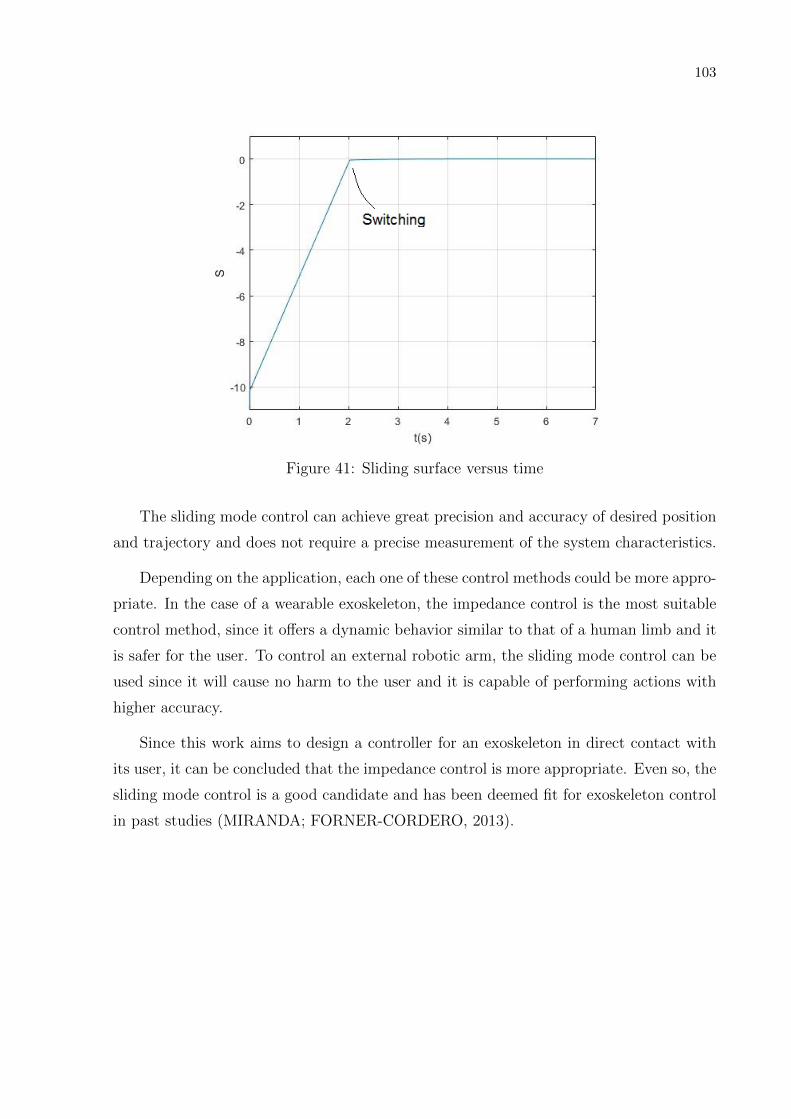
103
Figure 41: Sliding surface versus time
The sliding mode control can achieve great precision and accuracy of desired position
and trajectory and does not require a precise measurement of the system characteristics.
Depending on the application, each one of these control methods could be more appro-
priate. In the case of a wearable exoskeleton, the impedance control is the most suitable
control method, since it offers a dynamic behavior similar to that of a human limb and it
is safer for the user. To control an external robotic arm, the sliding mode control can be
used since it will cause no harm to the user and it is capable of performing actions with
higher accuracy.
Since this work aims to design a controller for an exoskeleton in direct contact with
its user, it can be concluded that the impedance control is more appropriate. Even so, the
sliding mode control is a good candidate and has been deemed fit for exoskeleton control
in past studies (MIRANDA; FORNER-CORDERO, 2013).

104
ANNEX A – SPARKFUN MUSCLE
SENSOR V3 SCHEMATIC

2/4/2013 1:03:11 PM H:\EMG\Muscle Sensor Platinum\v3\Muscle Sensor Platinum v3.3.sch (Sheet: 1/1)
123
123
4
1
58
7
2
3
REF
6
13
1214
411 2
31
6
57
9
108
12

106
ANNEX B – MODEXO CONTROL
HARDWARE SCHEMATICS

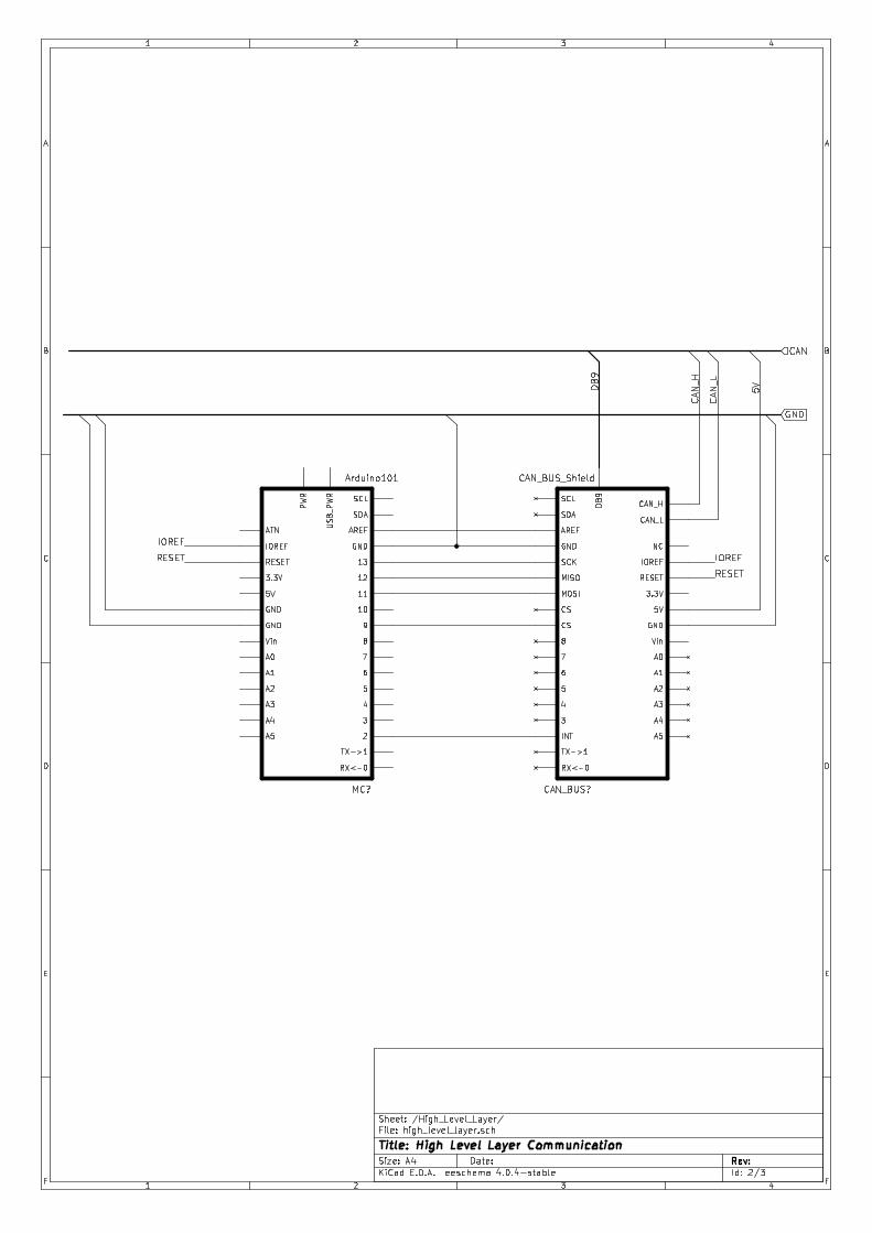
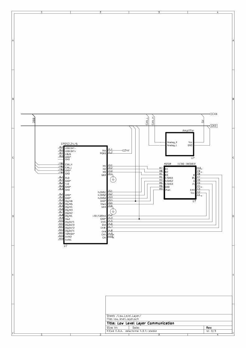


![NUOS Prescritores v1 [Modo de compatibilidad] · e innovaciones para el calentamiento de agua. PRO ECO ... NUOS SPLIT 80 – 110 150 3 ... agua a TSET del](https://img.dokumen.tips/doc/110x75/5baa96b909d3f2b2778c6b9c/nuos-prescritores-v1-modo-de-compatibilidad-e-innovaciones-para-el-calentamiento.jpg)


