EMERGY PERSPECTIVES ON THE ARGENTINE ECONOMY AND FOOD

EMERGY PERSPECTIVES ON THE ARGENTINE ECONOMY AND FOOD PRODUCTION SYSTEMS OF THE ROLLING PAMPAS

DURING THE TWENTIETH CENTURY

By

MARIA CECILIA FERREYRA

A THESIS PRESENTED TO THE GRADUATE SCHOOL OF THE UNIVERSITY OF FLORIDA IN PARTIAL FULFILLMENT

OF THE REQUIREMENTS FOR THE DEGREE OF MASTER OF SCIENCE

UNIVERSITY OF FLORIDA

2001

Copyright 2001

by

Maria Cecilia Ferreyra

To my beloved parents Mabel Valcarlos and Roberto Ferreyra

and

my dear husband Richard Hayman

iv

ACKNOWLEDGEMENTS

I would like to express my gratitude to each and everyone that made

possible my M.Sc. studies at the University of Florida. In particular, I would like

to mention the following people:

Dr. Mark T Brown, Dr. Clyde F. Kiker, and Dr. Stephen Humphrey, the

members of my committee at the University of Florida. Dr. Brown, my advisor,

introduced me to the emergy world and gave me support and guidance through

my university journey. Dr. Kiker, with his extensive experience in the economic

field, helped strengthen my understanding of national policies in Argentina. Dr.

Humphrey, the Dean of the College of Natural Resources and Environment of

the University of Florida (CNRE), through his vision and leadership, made

possible the interdisciplinary program in which this research was carried out.

My special appreciation goes to all the researchers at the National Institute

of Agricultural Technology of Argentina (INTA), whose valuable work of many

years provided most of the data for this study.

I would also like to acknowledge INTA, the Fulbright Commission (USA),

and the CNRE, for providing financial assistance. The Institute of International

Education (IIE) assisted me with logistics during my time in the USA. I thank all

of them.

v

TABLE OF CONTENTS

page

ACKNOWLEDGEMENTS............................................................................................. iv

TABLE OF CONTENTS .................................................................................................. v

LIST OF TABLES............................................................................................................vii

LIST OF FIGURES.............................................................................................................x

ABSTRACT ....................................................................................................................xiii

INTRODUCTION .............................................................................................................1

Statement of the Problem............................................................................................ 1 Emergy Accounting..................................................................................................... 2 The Argentine Case...................................................................................................... 4 Literature Review....................................................................................................... 10

Analysis of Nations................................................................................................ 10 Analysis of Food Production Systems ................................................................ 13

Plan of Study............................................................................................................... 17

METHODS .......................................................................................................................19

Description of Periods Analyzed............................................................................. 19 Argentina................................................................................................................. 19 Description of Farming Systems Analyzed........................................................ 21

Emergy Evaluation .................................................................................................... 23 General Procedure ................................................................................................. 23 Emergy Evaluation of Argentina’s Economy..................................................... 24

Data Gathering and Processing................................................................................ 28 Data Sources............................................................................................................ 28 Physical Flows........................................................................................................ 29 Money Flows........................................................................................................... 30 Human Services...................................................................................................... 30

vi

RESULTS ..........................................................................................................................32

Emergy Evaluation of the Economy of Argentina................................................ 32 The Overall Economy............................................................................................ 32 Renewable and Nonrenewable Inputs................................................................ 39 Indigenous Renewable Emergy Inputs............................................................... 44 Imports, Exports, and Balance of Payments....................................................... 45 Indices of Sustainability........................................................................................ 50

Emergy Evaluation of Agriculture in the Rolling Pampas .................................. 52 Intensive Agricultural Production in the Rolling Pampas............................... 52 Historical Evaluation of Agricultural Systems.................................................. 62 Emergy Indices of Agricultural Sustainability.................................................. 67

DISCUSSION ...................................................................................................................71

Argentina..................................................................................................................... 71 Rolling Pampas........................................................................................................... 76 Conclusions................................................................................................................. 82

APPENDIX

A ENERGY SYSTEMS SYMBOLS..........................................................................84

B SUMMARY OF DEFINITIONS AND CONCEPTS ........................................88

C EMERGY EVALUATION TABLES AND FOOTNOTES FOR ARGENTINA.............................................................................................90

D EMERGY EVALUATION TABLES AND FOOTNOTES FOR THE ROLLING PAMPAS......................................................................123

REFERENCES ................................................................................................................140

BIOGRAPHICAL SKETCH .........................................................................................149

vii

LIST OF TABLES

Table Page 1.1 Comparison of Per Capita GDP indexes (base= Argentina) and growth rates

between 1900 and 1997.....................................................................................5

2.1 National indices based on emergy analysis. .............................................................27

2.2 Emergy ratios for evaluation of economic use of resources. ..................................28

3.1. Annual emergy flows supporting the Argentine economy during the 1990-1995 period.........................................................................................................33

3.2. Summary of annual major emergy and monetary flows for Argentina during the 1990-1995 period.........................................................................................36

3.3. Overview indices of annual solar emergy use for Argentina during the 1990-1995 period.........................................................................................................37

3.4. Comparison of indigenous emergy uses in Argentina, expressed as percent of total indigenous emergy use. ..........................................................................44

3.5. Comparison of solar emergy indices of Argentina during the 20th century, including 1983 indices for USA and 1995 indices for Brazil.......................51

3.6. Comparison of solar emergy indices of Argentina during the 20th century, including 1983 indices for USA and 1995 indices for Brazil.......................53

3.7. Comparison of emergy indices for Argentina during the 20th century................54

3.8. Emergy evaluation of 1 ha of rain fed intensive agricultural production in the Rolling Pampas..................................................................................................56

3.9. Emergy evaluation of 1 ha of irrigated intensive agricultural production in the Rolling Pampas. ..........................................................................................57

viii

3.10. Emergy evaluation of 1 ha of no-tillage intensive agricultural production in the Rolling Pampas. ..........................................................................................58

3.11. Emergy indices for production systems of the Rolling Pampas during the 20th century, including corn production in Italy and bio-ethanol in Brazil. ..................................................................................................................68

4.1. External debt of Argentina during the 1980-1996 period.......................................76

C.1. Annual emergy flows supporting the Argentine economy during the 1900-1929 period.........................................................................................................90

C.2. Summary of annual major emergy and monetary flows for Argentina during the 1900-1929 period.........................................................................................95

C.3. Overview indices of annual solar emergy use for Argentina during the 1900-1929 period.........................................................................................................96








C.11. Summary of annual major emergy and monetary flows for Argentina during the 1976-1989 period............................................................................117

C.12. Overview indices of annual solar emergy use for Argentina during the 1976-1989 period................................................................................................118

ix

C.13. Footnotes for the emergy evaluation of the Argentine economy during the 1990-1995 period................................................................................................119

D.1. Emergy evaluation of 1 ha of low energy tenant farming production in the Rolling Pampas..................................................................................................126

D.2. Emergy evaluation of 1 ha of mixed grain and livestock farming production in the Rolling Pampas.......................................................................................128

D.3. Emergy evaluation of 1 ha of industrialized agricultural production in the Rolling Pampas..................................................................................................131

D.4. Footnotes for the emergy evaluation table of 1 ha of Rainfed intensive production system in the Rolling Pampas. ...................................................134

D.5. Footnotes for the emergy evaluation table of 1 ha of Irrigated intensive production system in the Rolling Pampas. ...................................................136

D.6. Footnotes for the emergy evaluation table of 1 ha of No-tillage intensive production system in the Rolling Pampas. ...................................................138

x

LIST OF FIGURES

Figure Page 1.1. Agricultural intensification in the Pampas. .............................................................1

1.2. Systems diagram of the environmental-economic interface..................................4

1.3. Map of Argentina.........................................................................................................6

1.4. Comparison of Per Capita GDP levels expressed in 1990 Geary-Khamis Dollars.................................................................................................................6

1.5. Ecological regions of Argentina. Pampean region (# 12) shown in dark green. 8

2.1. Pathways for evaluating the overall energy use of a state or a nation.................25

2.2. Aggregated diagram of emergy flows. .....................................................................26

3.1. Emergy diagram of Argentina. ..................................................................................35

3.2. Emergy signature of Argentina during the 20th century........................................38

3.3. Evolution of GDP and emergy/money ratio of Argentina during the 20th century................................................................................................................39

3.4. Evolution of emdollars and solar emjoules value of rain chemical potential Argentina during the 20th century..................................................................40

3.5. Systems diagram summarizing annual emergy (E+20 sej/y) and money flows (E+9 USD/y) for the 1990-1995 period in Argentina. .......................41

3.6. Contribution of renewable energy flows to national economies, including the 1990-1995 period for Argentina.......................................................................42

3.7. Partial emergy signature of Argentina during the 20th century............................43

3.8. Emergy input to Argentina’s economy during the 20th century resulting from main economic sectors......................................................................................46

xi

3.9. Contribution of imports to the total emergy budget of Argentina during the 20th century.........................................................................................................47

3.10. Main emergy import flows of Argentina during the 20th century.....................48

3.11. Main emergy export flows of Argentina during the 20th century.......................49

3.12. Emergy ratio of imports to exports in Argentina during the 20th century. .......50

3.13. Intensive food production systems in the Rolling Pampas. ................................55

3.14. Emergy value of net topsoil loss in the production systems of the Rolling Pampas during the 20th century......................................................................60

3.15. Emergy yields in the Rolling Pampas during the 20th century. ..........................61

3.16. Transformities for agricultural production in the Rolling Pampas during the 20th century.........................................................................................................62

3.17. Emergy input to agricultural systems in the Rolling Pampas during the 20th century................................................................................................................64

3.18. Empower density of agricultural production in the Rolling Pampas during the 20th century. .................................................................................................65

3.19. Relative importance of purchased inputs in the Rolling Pampas during the 20th century.........................................................................................................65

3.20. Relative importance of human labor in the Rolling Pampas during the 20th century................................................................................................................66

3.21. Percent renewable energy contribution to agricultural production in the Rolling Pampas during the 20th century........................................................69

3.22. Emergy yield ratio and Environmental loading ratio for agricultural production in the Rolling Pampas during the 20th century........................71

3.23. Emergy Index of Sustainabilty in the Rolling Pampas during the 20th century................................................................................................................70

4.1. Different scenarios stemming from product and input price conditions. ...........78

D.1. Low energy tenant farming production system in the Rolling Pampas.............123

xii

D.2. Mixed grain and livestock production system in the Rolling Pampas. ..............124

D.3. Agricultural industrialization production system in the Rolling Pampas. ........125

xiii

Abstract of Thesis Presented to the Graduate School of the University of Florida in Partial Fulfillment of the

Requirements for the Degree of Master of Science

EMERGY PERSPECTIVES ON THE ARGENTINE ECONOMY AND FOOD PRODUCTION SYSTEMS OF THE ROLLING PAMPAS

DURING THE TWENTIETH CENTURY

By

Maria Cecilia Ferreyra

December 2001 Chairman: Dr. Mark T. Brown Major Department: Interdisciplinary Ecology

Agricultural production in the Rolling Pampas of Argentina during the

20th century was characterized by the low use of external inputs. This tendency

changed during the 1990s with the widespread adoption of technological

innovation in the region. Macroeconomic policies implemented in Argentina in

the same decade, emphasizing free market and deregulation, contributed to the

selection of more efficient and cost-effective farming methods. In this context, the

sustainability of food production in the Rolling Pampas is becoming a concern.

The purpose of this research was to use Emergy Accounting as a

quantitative measurement of the ecological sustainability of agricultural

production in the Rolling Pampas during the 20th century. An alternative,

ecological interpretation of the history of the Argentine economy was also

xiv

attempted. For that purpose, emergy evaluations of modern and historical

agricultural systems and of the economy of Argentina were conducted. Emergy

balance of payments resulting from international trade and the international debt

of Argentina were also evaluated. Results were compared with past evaluations

of other countries and agricultural systems.

The emergy analysis of the Argentine economy throughout the 20th

century showed the influence of macroeconomic policies on sustainability.

Argentina started the century relying mostly on the use of renewable energy,

with nonrenewable energy increasing its importance as the economy developed.

As an exporter of commodities (oil, minerals, agricultural products), Argentina is

providing buyers more emergy than she receives in exchange. In emergy terms,

Argentina had already paid its external debt by 1985. In 1996, the accumulated

emergy value of total debt service represented 2.9 times the emergy of the total

debt stocks.

Liberal economic theory and trade liberalization have led to an increase in

the productivity of the agricultural sector, but has also increased the dependency

of farmers on external energy inputs. Policies towards the agricultural sector

should encourage the more sustainable among the possible options. Besides

adaptation of foreign technology to the local conditions, public research should

seek alternative, environmentally sound solutions. Emergy accounting, a

methodological tool that attempts to balance humanity and environment,

constitutes a useful tool for the evaluation of such policies.

1

CHAPTER 1 INTRODUCTION

Statement of the Problem

One of the main characteristics of agricultural production in the Rolling

Pampas of Argentina throughout the 20th century was the low use of external

inputs (Diaz Alejandro, 1970; Balze, 1995; Programa de Servicios Agricolas

Provinciales [PROSAP], 1997; Viglizzo et al., 2001). However, this tendency

changed during the 1990s, when intensification began to redefine the Pampean

agriculture (Figure 1.1). This farming “revolution” consisted principally of

adopting different technologies, such as fertilizers, pesticides, complementary

irrigation, and specific no-tillage machinery (PROSAP, 1997).

Figure 1.1. Agricultural intensification in the Pampas (Source: National Institute of Agricultural Technology [INTA], 1998).

2

A transformation of this magnitude cannot be understood in isolation. The

economic policies implemented under the presidency of Carlos Menem (1989-

1999), which emphasized free market and deregulation, contributed to the

selection of more efficient and cost-effective farming methods (PROSAP, 1997).

As a result, there is a trend in Argentina towards large-scale agricultural

operations that parallels the North American model that produces highly

technified monocultures (Quiñones, 1998; Pizarro, 1998; Obschatko, 1998). It is

within this context that the long-term prospects for sustainable food production

in the Rolling Pampas are becoming a concern.

The purpose of this research is to use Emergy Accounting as a

quantitative measurement of the ecological sustainability of agricultural

production in the Rolling Pampas during the 20th century. As such, it is intended

as a contribution towards present and future challenges for the region, ones that

must include not only productivity but also resource conservation as their

imperatives. An alternative, ecological interpretation of the history of the

Argentine economy will also be attempted. The ultimate goal is to add to the

discussion of sustainable development in Argentina, and to the evaluation of

national and regional policies and management practices towards that direction.

Emergy Accounting

Strategies towards sustainable development require appropriate

assessment methodologies. Ecological economics, a transdisciplinary field of study

3

that focuses on the relationships between ecological and economic systems,

offers such an integrated approach (Folke et al., 1994). One of the most important

research issues in ecological economics is natural resource valuation. Traditional

economic analysis does not include environmental degradation in performance

evaluations. Moreover, it does not take into account the contributions of nature

to human economies (Odum, 1994). As described by Brown and Ulgiati (1999),

these contributions encompass renewable energies (sunlight, tide), resource

flows (fuels, wood), and environmental services (waste assimilation, aesthetic

gratification). However, “money is only paid to people and never to the

environment for its work” (Odum, 1996, p 55).

Emergy Accounting is a science-based valuation system that incorporates

both environmental and economic values in a single measure: emergy (Odum,

1996). Emergy represents all the direct and indirect energies consumed in the

production of goods and services, including not only fossil fuel inputs but also

the work of nature (Figure 1.2).

Emergy Accounting constitutes a valuable tool for assessing the ecological

performance of countries and states. By allowing the valuation of human and

natural capital on a common basis, it offers an alternative for the inclusion of

environmental goods and services in systems of national accounts.

Emergy analysis has also been proposed as a methodology for the

assessment of agricultural sustainability within its ecological dimension

4

(Stachetti et al., 1998; Lagerberg, 1999). Inputs to food production systems

include environmental energies from both renewable sources and non-renewable

storages from past biosphere production (Stachetti et al., 1998). Therefore,

accounting for all contributions from nature becomes a necessary step towards

the implementation of sustainable agricultural systems.

Degraded Energy

EnvironmentalReserves

EnergySources:sun, windrain, tide

Natureproducingresources

StoredResources:water, soilminerals

EconomicUses

Waste

Purchases offuels, goods

and services

$

MainEconomy

Market

Figure 1.2. Systems diagram of the environmental-economic interface (Source: adapted from Odum, 1996, p. 59).

The Argentine Case

Argentina, the eighth largest country in the world, constitutes an

interesting case of study for economists and sociologists as well (Figure 1.3).

5

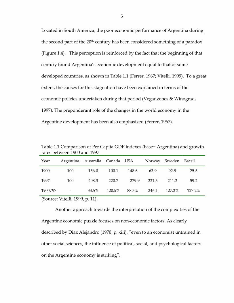
Located in South America, the poor economic performance of Argentina during

the second part of the 20th century has been considered something of a paradox

(Figure 1.4). This perception is reinforced by the fact that the beginning of that

century found Argentina’s economic development equal to that of some

developed countries, as shown in Table 1.1 (Ferrer, 1967; Vitelli, 1999). To a great

extent, the causes for this stagnation have been explained in terms of the

economic policies undertaken during that period (Veganzones & Winograd,

1997). The preponderant role of the changes in the world economy in the

Argentine development has been also emphasized (Ferrer, 1967).

Table 1.1 Comparison of Per Capita GDP indexes (base= Argentina) and growth rates between 1900 and 1997

Year Argentina Australia Canada USA Norway Sweden Brazil

1900 100 156.0 100.1 148.6 63.9 92.9 25.5

1997 100 208.3 220.7 279.9 221.3 211.2 59.2

1900/97 - 33.5% 120.5% 88.3% 246.1 127.2% 127.2%

(Source: Vitelli, 1999, p. 11).

Another approach towards the interpretation of the complexities of the

Argentine economic puzzle focuses on non-economic factors. As clearly

described by Diaz Alejandro (1970, p. xiii), “even to an economist untrained in

other social sciences, the influence of political, social, and psychological factors

on the Argentine economy is striking”.

6

Figure 1.3. Map of Argentina. (Source: National Geographic Cartographic Division, 1995).

0

5000

10000

15000

20000

25000

1900 1920 1940 1960 1980

Time

Per C

apit

a G

DP

(199

0 do

llar

s)

Argentina

Australia

Canada

Norway

Sweden

USA

Figure 1.4. Comparison of Per Capita GDP levels expressed in 1990 Geary-Khamis Dollars (Source: Maddison, 1995, Appendix D).

7

Argentina’s economic history cannot be separated from its natural

resource base. A nation abundant in resources and land, Argentina started the

century as a leader in agricultural exports (Giberti, 1988; Veganzones &

Winograd, 1997). The country still benefits from the exceptional Pampean

Region1 (Figure 1.5), a fertile agricultural plain of almost 55 million hectares and

temperate climate (Giberti, 1988). The relevance of the Pampas for the national

economy can be explained in part by the fact that the region (1) gives the country

substantial gains in terms of export earnings, (2) accounts for great part of the

population’s food requirements, and (3) constitutes an important source of state

revenue through export retentions (Busnelli, 1992). The Rolling Pampas, the most

productive area within the region, accounts for a great part of these three aspects.

Argentina is also rich in energy reserves, including oil and natural gas (EIA,

2000a). Water resources are being developed at a rapid rate. Currently,

Argentina relies mostly on hydropower and natural gas to fuel its electricity

sector (EIA, 2000a).

Argentina was in 1997 the world largest exporter of sunflower flour and

sunflower and soy oil and the second largest exporter of maize, sorghum, and

soy flour (Solá, 1997). Nevertheless, oil, gas and electricity are growing in

importance as exports. It is estimated that Argentina could become the major

energy supplier of the Southern Cone region (EIA, 2000a).

1For a detailed description of the Pampean Region, refer to Barsky (1991).

8

Figure 1.5. Ecological regions of Argentina. Pampean region (# 12) shown in dark green (Source: Sistema de Informacion Ambiental [SIA], 2001).

9

The trade balance tends to be favorable to Argentina when world demand

for food is high. Export growth slowed sharply in 1998 due to lower world prices

for petroleum and agricultural commodities (US State Department, 1999).

MERCOSUR, the regional customs union of the Southern Cone that includes

Argentina, Brazil, Paraguay and Uruguay, has proven to be very important for

the country’s trade. However, there has been escalating stress after the Brazilian

devaluation in 1999 (Australian Department of Foreign Affairs and Trade

[ADFAT], 2001).

Argentina's external debt to GDP ratio is the highest among the three

largest economies of Latin America (Mexico, Brazil, and Argentina). In 1998, this

ratio was approximately 47% of annual GDP. While Argentina’s external debt to

GDP ratio is the highest, the external debt is the lowest. In 1998 debt service as a

percentage of all exports for the same year was significantly lower than it was at

the outset of the 1980s debt crisis (Janada, 1999).

The current state of Argentina’s environment, as in the case of its

economy, is rather disappointing. Soil erosion, deforestation, and water

contamination are some of the consequences of a development style that chose

not to -or was not able to- conserve the quality of its vast natural resources

(Ministerio de Economia [MECON], 2000). Environmental degradation in

Argentina has been a matter of analysis in numerous studies (Brailovsky and

Foguelman, 1991; Secretaria de Recursos Naturales y Ambiente Humano

10

[SRNyAH], 1992; Vila and Bertonatti, 1993; World Bank, 1995; Programa

Cooperativo para el Desarrollo Tecnologico Agropecuario del Cono Sur

[PROCISUR], 1997; PROSAP, 1997). However, the assessment and quantification

of the interrelations between environment and economy remain a complex task.

Emergy Accounting goes beyond the artificial boundaries of

socioeconomic systems and acknowledges the intricate relationships between

human societies and the biosphere. It brings a more holistic perspective to the

sustainability issue, and in doing so, becomes a useful methodological tool for

the incorporation of environmental concerns to the policy making process of the

Rolling Pampas and the rest of Argentina.

Literature Review

Analysis of Nations

In the past two decades, the field of environmental accounting for nations

has aroused increasing attention around the world (Hecht, 1999). Repetto et al.

(1989) adjusted Indonesia’s GDP by including the net depletion of some of the

country’s natural resources. After petroleum, timber, and soils exploitation was

considered, the estimated annual net domestic product (NDP) for the 1971-1984

period was almost 40% less than the conventionally measured GDP.

Peskin (1989) focused on the accounting of forest resources to alter the

1980 conventional accounts for Tanzania. The accounting framework used by the

11

author was based on neo-classical economic theory (Peskin and Lutz, 1990).

According to the results, that natural forest depreciation had no effect on the

country’s GDP, but lowered the NDP by about 5%.

Tongeren et al. (1993) adapted the UN’s System of Integrated

Environmental and Economic Accounts (SEEA) for Mexico. Using

environmentally adjusted NDP measurements they showed increases in final

consumption and decreases in net capital accumulation and environmental

assets.

Bartelmus et al. (1993) used the same approach for the evaluation of Papua

New Guinea. For the 1986-1989 period the authors found that environmentally

adjusted NDP reduces NDP levels by amount ranging from 1 to 10%.

Oda et al. (1998) applied the SEEA to the Japan economy for 1985 and

1990. They found that for that period the environmentally adjusted product

increased 0.1% more than the conventional NDP. Kim et al. (1998) used a similar

approach to study the 1985-1992 period for the Republic of Korea. They found an

increase in the share of environmentally adjusted product to NDP.

The analysis of Philippines by Domingo (1998) revealed depletion in that

economy decreased from around 4% in 1988 to less than 1% in 1992. The author

found the SEEA framework adequate for environmental accounting.

Keuning and de Haan (1998) showed the National Accounting Matrix

including Environmental Accounts (NAMEA) results for the Netherlands. This

12

methodology contains a complete system of national flow accounts including

emissions of pollutants, extraction of natural resources, and their effects.

According to the authors, total pollution per unit of final demand decreased form

1987 to 1992. In the later year, more than half the greenhouse effect, the

acidification, and the eutrophication were caused by industries that generated

less than 10% of GDP. At a more detailed level, NAMEA showed that most

wastes were generated by exports. Direct pollution by the chemical industry and

total environment intensity of the final demand for chemical products were

substantially above average.

Emergy Accounting has been used to evaluate different national

economies from a large-scale perspective. An overview of these studies was

given by Odum (1996), along with a complete evaluation of the USA for 1983.

Results for the US economy were consistent with what was expected for a

developed economy, with less than 10% of total emergy derived form locally

renewable sources.

Brown (1998) used the same methodology to evaluate Chile’s performance

during 1994. The emergy analysis indicated a relatively sustainable economy,

because of the relatively high levels of renewable energy flows obtained form

within the country. However, Chile showed a negative emergy balance of

payments, exporting about 1.66 times as much emergy as is imported.

13

An emergy evaluation of the Brazilian economy during 1995 showed a

transitional state between a developed and undeveloped economy. High use of

renewable energy and low import of purchased emergy and materials

characterized Brazil as a highly self-sufficient economy.

Lagerberg et al. (1999) used emergy accounting to evaluate the Swedish

economy for 1988 and 1996. They found that the 30% growth in the total

economy was based on greater use of local resources, and an even greater

increase in imported goods and services. Renewable resources were considered

constant over the period, and the environmental loading increased due to the

greater reliance on non-renewable resources.

Analysis of Food Production Systems

Most researchers agree on the essential role of quantitative evaluation in

the agriculture sustainability issue (Smit and Smithers, 1991; Hailu and Runge-

Metzger, 1992; Stachetti et al., 1998; Sands and Podmore, 2000). However,

attempts towards the appraisal of sustainability in agriculture have been

hindered by conceptual inconsistencies and lack of practical definitions

(Brklacich et al., 1991; Sands and Podmore, 2000).

Franzluebbers and Francis (1995) determined the energy output: input

ratio of several maize and sorghum management systems in eastern Nebraska.

They concluded that rotation of cereals and legumes under dryland conditions in

the western Corn Belt may be more sustainable for the future based on energy

14

use efficiency of lower fossil fuel requirements from N fertilizer and irrigation.

Ramirez and Martinez (1995) studied the assessment of the sustainability

of peasant production systems focusing on soil erosion in Chile. Using neoclassic

economic theory, they found a trade off between erosion and farm returns in one

of the regions under analysis.

Viglizzo et al. (1998) studied the trade-offs between productivity, stability,

and sustainability during one century of low external-input farming in the

pampas of Argentina. Comparing components, diversity patterns, and

connectance of farming systems they found that productivity had increased all

over the region at the expense of stability and sustainability.

Hellkamp et al. (1998) measured the condition and sustainability of

agricultural lands in five Mid-Atlantic states in 1994. Using indicators of crop

productivity and land stewardship on annually harvested herbaceous cropland,

they found that the overall condition in the region was good.

Halberg (1999) developed a set of farm level indicators of environmental

impact that was tested on 20 Danish dairy and pig farms. Included were the

surplus and efficiency of N, P and Cu, the energy use per kg grain and per kg

milk or meat, pesticide treatment index and indicators of nature quality. The

indicators reflected differences in management practices on comparable farms.

Bouman et al. (1999) used SOLUS (Sustainable Options for Land Use), a

framework for (sub-) regional land use that quantifies biophysical and economic

15

sustainability trade-offs, in Costa Rica. SOLUS consists of technical coefficient

generators, a linear programming model, and a geographic information system.

Results showed that introduction of alternative technologies may sometimes

satisfy both economic and biophysical sustainability. However, negative trade-

offs were found among different dimensions of biophysical sustainability.

Sands and Podmore (2000) propose a generalized sustainability index for

agricultural systems. A case study was developed based on prevalent corn and

wheat agricultural production systems in Baca County (Colorado). For all the soil

types being evaluated, the corn system was the least sustainable. Rotational

systems were found to be more sustainable than the other two continuous-crop

management systems. In general, the degree of distinction among soil types

regarding sustainability was much less pronounced than that exhibited among

crop management systems.

Tellarini and Caporali (2000) used an input/output methodology to

evaluate farms as sustainable ecosystems in both energy and monetary values in

Central Italy. They found differences between low and high-input farming

systems, but concluded that energy and monetary values did not offer a single,

coherent account of the functioning of farm systems.

Andreoli and Tellarini (2000) used a simplified approach for farm

sustainability evaluation in Tuscany. Results showed that farms might have very

different performances according to the way they are managed, regardless of

16

their location. Since some productive types were less environmentally

satisfactory, they concluded that it is important to find relatively positive styles

of farming for these production types.

Di Pietro (2001) studied sustainable land use in agriculture at the

landscape level in France. Indicators of sustainability were based on the

contribution of the environment to the choice of agricultural practices by

farmers, and on relationships between agro-ecological units and farms. Results

showed that ecological sustainability of larger territories seemed to be in

opposition with the standard criteria judging economical sustainability of farms.

Xu and Mage (2001) presented a preliminary case study of southern

Ontario using a model of agroecosystem health. They found that the overall level

of structural and organizational health of the agroecosystem has declined in that

area. However, functional health had improved greatly. The maintenance of

agroecosystem function and structure in the study region had become

increasingly dependent upon external inputs.

As in the case of analysis of national economies, Emergy Accounting has

been used to evaluate ecological performance of different agricultural production

systems. Odum (1984) studied corn production in USA and found that modern

agriculture is based on massive contributions of emergy.

Lagerberg et al. (1999) used the same approach to assess the sustainability

of greenhouse tomatoes in Sweden. The intensive tomato production system

17

investigated was shown to be highly dependent on non-renewable resources and

human service fed-back from the economy.

Using Emergy accounting, five different Swedish greenhouse tomato

production systems were analyzed by Lagerberg et al. (1999). Conventional

systems were shown to utilize resource inputs more efficiently than organic

systems due to higher yields of the formers. They concluded that replacing fossil

fuels with more renewable fuels is an important strategy for the sustainability of

tomato production systems.

Plan of Study

To evaluate agricultural production in the Rolling Pampas and to gain

insight into its sustainability, emergy evaluations were conducted of modern and

historical agricultural systems. To place in perspective the role of the Pampas

agriculture in the national economy and effects of international trade on

production, the economy of Argentina was evaluated using emergy. Emergy

balance of payments resulting from international trade and the international debt

of Argentina were also evaluated.

Historical data on the economy of Argentina and agricultural production

in the Rolling Pampas were collected from a variety of sources. Five time periods

were analyzed as “typical” windows of economic and technological

characteristics. Data were averaged using these windows. The economy of

18

Argentina and agricultural systems of the Rolling Pampas were compared with

other countries.

Using data on international debt and the emergy buying power of the

Argentine economy, as well as emergy per dollar of exports, an emergy debt

service was calculated to evaluate the relative position of Argentina with regard

to its international debt.

19

CHAPTER 2 METHODS

The methodological approach undertaken in this study consisted of an

emergy evaluation of the economy of Argentina during five time periods. Food

production systems of the Rolling Pampas, characteristic of these same time

periods, were also evaluated. First a general description of the time periods is

given, followed by a description of the agricultural production systems.

Description of Periods Analyzed

Argentina

Five stages of economic development were analyzed, following the model

proposed by Veganzones & Winograd (1997).

- 1900-1929: The Golden Age of Argentine Growth. - 1930-1943: The World Depression and Destabilization of the Argentine

Model. - 1944-1975: Import Substitution and Increasing Economic and Political

instability. - 1976-1989: The Attempt to Liberalize the Economy, the Debt Crisis and

Extreme Macroeconomic Volatility. - 1990-1995: Hyperinflation and Change in the System. Return of Sustainable

Growth?

20

The reliance on economic interpretation for the selection of the study

periods acknowledged the interdependence of natural capital and economic

development. Moreover, the selection was made with the purpose of attaining

another perspective for that economic history, incorporating the point of view of

Emergy Accounting. A detailed description of each of the five periods can be

found in Veganzones and Winograd (1997). A synthesis based on the work of

these authors follows.

The rapid growth that had begun in the early 1880s continued in the 1900-29 period. . . . This growth was closely linked to rising exports and investment . . . agriculture was the most important sector. . . . State intervention in the economy was limited. . . . The country was heavily dependent on the free flow of merchandise and capital (p 24). . . . The 1930s crisis revealed the fragility of the development model chosen by Argentina. . . . Awareness of this fragility led the country’s leaders in 1943 to adopt an import-substitution policy. . . . Against a background of chronic and accelerating inflation, economic and political instability arising primarily from existing policies, led to loss of control of the economy by the early 1970s (p 33). . . . The 1975 breakdown marked the definitive limit of the import-substitution regime. . . . By 1981 the military government’s mishandling of its stabilization programmes and economic liberalisation policy had plunge the country into a serious crisis of unprecedented length . . . liberalisation was gradually reintroduced by the Radical Government elected in 1983. . . . The high degree of instability and demonetisation of the economy resulted in two bouts of hyperinflation: one in 1989, under the Radicals; and another in 1990, during the Peronist government (p 38). . . . In this short period from 1990 to 1995, economic performance was exceptional compared to the two preceding decades. . . . Profound economic reforms were undertaken that set in motion a change in growth strategy. Liberalisation of the economy was completed and stabilization was achieved. It may be too soon to announce the complete success of the reforms; the slow recovery of financial intermediation and the financial crisis of 1995 are signs that the economy is still fragile (p 40).

21

Description of Farming Systems Analyzed

Four stages of the evolution of the Rolling Pampas during the 20th century

were identified, based on the work by Giberti (1988) and Pizarro (1998):

- Agricultural predominance. From 1900 to 1940 tenant farmers, most of them immigrants without capital coexisted with colonial ranchers. Ranchers, owners of enormous extensions of land devoted to cattle raising, lent fields to farmers for crop production for three years. Farmers would turn the field into alfalfa pastures before moving to the next field, and paid a percent of the harvest to the owner. As the international prices of the grains increased, large landowners reduced their herds, and tenants were in demand not for the alfalfa fields but for the income from grain production.

- Mixed Farming. After World War II Argentine grain was left without foreign

markets. Farmers who own their land incorporated livestock to diversify production. Tenants, limited by their contracts did not have this option. Legal measures and political transformations improved the conditions of landless farmers. By 1960, most of the land was being farmed by its owners. During this period, mechanization replaced human and animal labor.

- Agriculturization. A strong predominance of grain over cattle characterized

this stage. The introduction of soybean in the 1970s allowed a double crop in the same calendar and led to a propensity towards continuous agriculture. Technological innovations, such as improved genetic material, pesticides, and specialized machinery, improved the general productivity. However, soils suffered the consequences of such pressure.

- Intensification. This is the current stage, which started in the 1990s.

Management skills and production scale are as important as technological innovation to produce in the competitive global market.

The dominant agricultural systems that characterized these four periods

in the Rolling Pampas were evaluated: Low energy tenant farming (1900-1940),

Mixed grain and livestock production (1940-1970), Agricultural industrialization

(1970-1990), and Agricultural Intensification (1990-). Since recently irrigation and

no-tillage methods of farming have gained importance in the Rolling Pampas,

22

three different n production systems were evaluated for the Agricultural

intensification period: (1) Rainfed-intensive agriculture, (2) Irrigated-intensive

agriculture, and (3) No-tillage intensive agriculture. The main technical

characteristics of these production systems follow.

- Low energy tenant farming. Tenant farmers worked 80 ha in the north of the province of Buenos Aires. Of the total land area, 25 ha were planted flaxseed, 50 ha corn, and the rest was used for grazing of draft animals. The capital consisted of 20 Creole horses, and some agricultural machinery. The system yielded 150,000 kg of corn and 20,000 kg of flaxseed. (Source: Ministerio de Agricultura, 1929)

- Mixed grain and livestock production. Landowners worked 100 ha in the

north of the province of Buenos Aires, using the following rotation: 4 years of corn production, 2 years of wheat and sunflower, and 5 years of grassland for cattle raising. About 70% of the total land is under crop cultivation; the rest is for livestock production. The system yielded annually 3,100 kg of corn, 2,200 kg of wheat, 1,000 kg of sunflower, and 182 kg of meat per ha. (Source: Pereyra and Tricco; 1968; Kugler and Nocetti, 1969)

- Agricultural industrialization. Landowners worked 100 ha in the north of

the province of Buenos Aires, devoted mainly to soybean production. Around 35% of the land is planted with soybean, 35% with soybean combined with wheat, and the rest is for corn production. The system yielded 4,500 kg of corn, 2,500 kg of wheat, and 2,000 kg of soybean per ha. (Source: Pizarro and Cacciamani, 1980; Barsky, 1988)

- Rainfed-intensive agriculture. Medium-size farms (100 to 500 ha) in the

north of Buenos Aires are devoted to corn, wheat and soybean production (50% of the land area for corn production, 50% with soybean or soybean combined with wheat). Fertilizers were used for the first two crops. The system yielded 7,000 kg of corn, 4,000 kg of wheat, and 3,200 kg of soybean per ha. (Source: PROSAP, 1997)

- Irrigated-intensive agriculture. Similar to the rain fed intensive system, but

irrigation was also used as an input to the system. Irrigation accounted for 120, 90, and 100 mm of the water requirements of corn, wheat, and soybean, respectively. The system yielded 13,000 kg of corn, 6,000 kg of wheat, and 3,500 kg of soybean per ha. (Source: PROSAP, 1997)

23

- No-tillage intensive agriculture. Similar to the rain fed intensive system, but specific no-tillage machinery was used in all the crops of the rotation. The system yielded 6,000 kg of corn, 2,900 kg of wheat, and 3,200 kg of soybean per ha. (Source: Daza, 1998)

Emergy Evaluation

Emergy evaluations of Argentina and the selected food production

systems were based on the environmental accounting methodology set out by

Odum (1996).

General Procedure

- Delimitation of boundaries and elaboration of a systems diagram representing the main components and energy sources.

- Identification of relevant processes. These may comprise flows, interactions,

production, consumption, and money transactions. - Development of evaluation tables for emergy flows. - Elaboration of aggregated summary tables and diagrams for the emergy

flows. - Computation of emergy based parameters and indices.

Emergy Analysis has been described in great detailed elsewhere (Odum,

1994, 1996; Brown, 1998; Brown and Ulgiati, 1999). A summary of the main

energy systems symbols used for emergy diagrams is given in Annex A. An

overview of the basic emergy concepts and definitions is presented in Annex B.

24

Emergy Evaluation of Argentina’s Economy

Emergy driving the Argentine economy comes from three main sources,

as follows:

- Renewable inputs of biospheric emergy (outside sources), - Imported, non-renewable sources (purchased goods, fuels, services), and, - Indigenous non-renewable energy sources (soils, wood, fuels harvested from

within Argentina).

These inputs were evaluated for each of the time periods described above

using mean data for each time period. A summary of aggregated flows is

presented in Figure 2.1, including the circulation of money. Using this figure as a

guide, the following inputs and exports were evaluated:

Renewable inputs (R) include sunlight, wind, waves, tidal influence, rain,

and geologic contributions of the land. All renewable inputs were evaluated, but

only the largest was used in subsequent evaluations and indices to avoid double

counting. Non-renewable resources originated within the country’s boundaries

comprise:

- N0, rural resources used faster than their regeneration rate, - N1, the reserves of fuels and minerals, and, - N2, resources passing through the country economy without appreciable

transformation (emergy of these commodities is not considered as an emergy contribution to the nation economy).

Imports included flows of energy (F), goods that have emergy in addition

to services involved (G), and total imported services (P2I). In general, the emergy

25

of imported services was estimated using the monetary value and the

emergy/money ratio of the country of origin. Exports, comprised of resources

(N2), goods (B), and services (P1E), were also evaluated. The emergy exported as

services (P1E3) was estimated using the monetary value of exports and the

emergy/money ratio of Argentina for the year of the evaluation.

Soils,wood

Fuels,minerals

Sun,rain,wind

Goods

Services

Markets$

GDP

Fuels,minerals

R B

No

N1

F

N2

F' G'

G

P2I

I

P1E3P1E

E

P2I3I3

Ruralrenewable

Figure 2.1. Pathways for evaluating the overall energy use of a state or a nation (Source: adapted from Odum, 1996, p. 198).

26

A summary of national parameters and indices based on the main emergy

inflows and outflows of Argentina is given in Table 2.1. Further aggregation of

main flows (Figure 2.2) in indigenous sources (I= R+N), purchased inputs (F= M+S),

along with the flow of yields, allows the calculation solar transformities and other

emergy based sustainability ratios given in Table 2.2.

Degraded Energy

LocalRenew.Sources

EconomicUses

Purchased Resources

MainEconomy

LocalNon-renew.

Sources

Services

OtherSources

Y= Yield

R

NM

S

Figure 2.2. Aggregated diagram of emergy flows (Source: Odum, 1996, p. 83).

Solar transformities of final products were obtained by dividing the total

solar emergy of inputs (I + F) by the available energy of the yield (Y). Of special

interest is the Emergy Index of Sustainability (formerly known as Emergy

Sustainability Index). According to Brown (1998), the EIS summarizes the main

aspects of ecological sustainability: yield, renewability, and load on the

environment.

27

Table 2.1 National indices based on emergy analysis.

Name of Index Expression

Renewable Emergy flow R

Indigenous nonrenewable reserves N

Flow of imported emergy F + G + P2I3

Total emergy inflows R + N + F + G + P2I3

Total emergy used, U N0 + N1 + R + F + G + P2I3

Total exported emergy N2 + B + P1I3

Fraction of emergy used derived from local sources (NO + N1 + R)/U

Imports minus exports (F + G + P2I3) – (N2 + B + P1I3)

Ratio of exports to imports (N2 + B + P1I3)/ (F + G + P2I3)

Fraction used, locally renewable R/U

Fraction of use purchase (F + G + P2I3)/U

Fraction used, imported service P2I)/U

Fraction of use that is free (NO + R)/U

Ratio of concentrated to rural (F + G + P2I3 + N1)/(R +NO)

Use per unit area U/area

Use per capita U/population

Renewable carrying capacity at present living standard (R/U)(population)

Developed carrying capacity at same living standard 8(R/U)(population)

Emergy/money ratio (ratio of use to GDP) F1 = U/GDP

Ratio of electricity to use Electricity/U

Fuel use per capita Fuel/population

(Source: Odum, 1996, p. 199)

28

Table 2.2 Emergy ratios for evaluation of economic use of resources.

Name of Index Expression

Percent Renewable (% Renew) R/(R+N+F)

Emergy Yield Ratio (EYR) Y/F

Environmental Loading Ratio (ELR) (F+N)/R

Emergy Index of Sustainability (EIS) EYR/ELR

(Source: Brown, 1998)

Finally, the environmental emergy signature of the country was determined.

It represents the relative importance of the energy flows for that country

expressed in the common basis of emergy. The procedure consisted of plotting

the emergy flows in a bar graph, according to increasing transformities.

Data Gathering and Processing

Data Sources

Most of the data for the evaluation of Argentina were obtained from

published sources that account for the evolution of the country throughout the

century analyzed. Data corresponding to more recent years were also obtained

from databases maintained by public institutions of Argentina, such as the

Ministry of Economy (MECON) and the National Institute of Statistics (INDEC),

and from international and foreign organizations, such us the Food and

Agricultural Organization (FAO) and the Energy Information Administration

(EIA) of the United States.

29

National emergy-based indices of other economies for comparative

purposes were obtained from past studies, especially those concerning

MERCOSUR1 countries (Kent, 1996; Brown, 1998; Brown et al., 2000; Ferreyra,

2000).

Regarding food production in the Rolling Pampas, information was

obtained mainly from technical papers and reports prepared by the National

Institute of Agricultural Technology (INTA), and the Secretariat of Agriculture,

Fisheries, and Food (SAGPyA).

Physical Flows

All flows across the Argentine boundary –inputs and exports- were

expressed in physical units. Data series for the 20th century were used to obtain

the annual average inflows and outflows for each evaluation period. In case of

missing data, averages from available years were used. In the case of the Rolling

Pampas, physical information of inputs, outputs, and yields reflected the

common production practices at the different stages in the evolution of the area.

In both cases, inflows and outflows were transformed to joules of energy

using the corresponding caloric contents on a dry weight basis. Minerals,

chemicals, and machinery data were expressed as dry weight units. All

calculations and data sources are given in the footnotes of the emergy evaluation

tables.

1MERCOSUR is the common name of the Southern Common Market, a customs union formed by Argentina, Brazil, Uruguay, and Paraguay in 1991. Free trade agreements were signed with Chile and Bolivia in 1996 and 1997 respectively.

30

Values of transformities were taken from past studies, especially those

from Odum (1996) and Brown (1998). These transformities were used to

transform energy values to units of emergy (solar emjoules).

Money Flows

GDP was expressed in constant dollars in order to reduce distortions

caused by inflation. This information, along with population data, was obtained

from the work by Maddison (1995), which provided a comprehensive economic

database for fifty-six countries over the period from 1820 to 1992, among them

Argentina. Maddison used the Geary-Khamis approach to transform annual

GDP levels into a common unit, 1990 dollars. A detailed description of the

methodology, as well as the information sources used for Argentina’s GDP

estimations can be found in Maddison (1995).

Emergy value of international loans was calculated by multiplying the

monetary value of the loans by the world emergy/money ratio. The emergy

value of external debt service was evaluated using the annual monetary

payments multiplied by the national emergy money ratio for that period. A ratio

of emergy in loans to emergy value of debt repayment was calculated using the

emergy of loans and emergy of total payments.

Human Services

Emergy/money ratios of Argentina, obtained as a result of the emergy

evaluations, were used to estimate the transformity for human labor in the

31

Rolling Pampas. According to Odum (1996), this transformity can be calculated

by dividing the total emergy use for a country by its working population. The

resulting emergy per person is then distributed using the number of hours per

calendar year.

Emergy in human services related to the production of hybrids and

genetically modified seeds for agricultural production was estimated by

calculating the difference in price between seeds and yields, and multiplying the

result for the emergy/money ratio of Argentina for the corresponding time

period.

32

CHAPTER 3 RESULTS

Emergy Evaluation of the Economy of Argentina

The Overall Economy

A summary diagram for the Argentine economy is shown in Figure 3.1. It

identifies main inflows of environmental energies as well as relevant indigenous

resources and production processes within the country. An emergy evaluation

for the 1990-1995 period of the Argentine economy is given in Table 3.1.

Summaries of aggregated flows and national indices are presented in Tables 3.2

and 3.3 respectively. Evaluation and summary tables for four historical periods

(1900-1929, 1930-1943, 1944-1975, 1976-1989) that were also evaluated can be

found in Annex C. The evolution of the emergy signature of Argentina during

the 20th century, shown in Figure 3.2, was compiled based on the detailed

analysis given in these tables.

The contribution of renewable resources-sunlight, rain, wind, waves,

tides, and earth cycle- to the economy were considered to remain constant

throughout the century. Since local renewable emergy inputs are coproducts of

the main geobiospheric processes of the earth, their emergies are not

independent (Odum, 1996). In order to avoid double counting only the largest

33

one, rainfall chemical potential, was used to obtain the emergy flow of renewable

resources for each period (item R on summary flow tables).

Table 3.1. Annual emergy flows supporting the Argentine economy during the 1990-1995 period.

Note Item Raw Unit Emergy/unit Solar Emergy EmDollars (sej/unit) (E20 sej) (E9 1990 US$)

Renewable resources:

1 Sunlight 1.68E+22 J 1.00E+00 167.99 8.60

2 Rain, chemical 1.47E+19 J 1.82E+04 2680.46 137.18

3 Rain, geopotential 7.03E+18 J 2.79E+04 1958.65 100.24

4 Wind, kinetic energy 2.07E+19 J 1.50E+03 309.67 15.85

5 Waves 8.05E+17 J 3.06E+04 245.93 12.59

6 Tide 3.19E+18 J 1.68E+04 538.03 27.54

7 Earth Cycle 2.78E+18 J 3.44E+04 955.82 48.92

Indigenous renewable energy:

8 Hydroelectricity 9.67E+16 J 1.65E+05 159.49 8.22

9 Agriculture Production 1.39E+17 J 1.00E+05 138.57 7.14

10 Livestock Production 4.65E+16 J 1.00E+06 465.32 23.97

11 Fisheries Production 3.44E+15 J 1.00E+06 34.40 1.77

12 Fuelwood Production 4.38E+10 J 1.87E+04 0.00 0.00

13 Forest Extraction 4.75E+16 J 1.87E+04 8.89 0.46

Nonrenewable sources from within system:

14 Natural Gas 1.02E+18 J 4.80E+04 491.43 25.15

15 Oil 1.43E+18 J 5.40E+04 770.32 39.42

16 Coal 7.65E+15 J 4.00E+04 3.06 0.16

17 Minerals 4.82E+13 g 1.00E+09 482.34 24.69

18 Metals 2.02E+11 g 1.00E+09 2.02 0.10

19 Top Soil 1.70E+17 J 7.40E+04 125.45 6.42

34

Table 3.1 (continued)


Imports and outside sources:

20Oil Derived Products 1.06E+17J 6.60E+04 70.04 3.61

21Metals 9.91E+11g 1.80E+09 17.85 0.92

22Minerals 4.41E+12g 1.00E+09 44.14 2.27

23Food & Ag Products 1.34E+16J 2.00E+05 26.70 1.38

24Coal 3.63E+16J 4.00E+04 14.54 0.75

25Plastics & Rubber 1.21E+16J 6.60E+04 7.97 0.41

26Chemicals 1.88E+12g 3.80E+08 7.15 0.37

27Wood,Paper,Textiles 1.29E+16J 3.49E+04 4.49 0.23

28Mech.& Trans Eqp. 7.40E+11g 6.70E+09 49.60 2.56

29Service in imports 3.23E+10$ 1.24E+12 401.10 20.66

Exports:

30Agricultural Crops 8.72E+16J 2.00E+05 174.40 8.98

31Fishery Products 4.95E+13J 1.00E+06 0.49 0.03

32Forest Products 6.71E+15J 3.49E+04 2.34 0.12

33Crude Oil 4.78E+17J 5.30E+04 253.12 13.04

34Metals / Minerals 1.57E+13g 1.00E+09 156.69 8.07

35Paper & Wood 9.17E+15J 3.49E+04 3.20 0.16

36Chemicals 5.93E+11g 3.80E+08 2.26 0.12

37Service in exports 2.74E+10$ 1.94E+12 531.28 27.37 38Service external debt 9.31E+09$ 1.94E+12 180.63 9.31

Calculations and references for basic data are given in Appendix C.

35

Sun

Wind

Rain

RiversEarthCycle

Oil

Minerals

Gas

Goods &Services

GDP$

Info

Loans Aid

Foreignmarkets

$

ForestsGrasslandsParks

Water

Soils

Pampeanregion

Industry

Commerce

Waste

Mining Hydroelectricpower

Govt.

People

Transport

Extrapampean

region

Figure 3.1. Emergy diagram of Argentina.

36

Table 3.2. Summary of annual major emergy and monetary flows for Argentina during the 1990-1995 period.

Variable Item Dollars

Solar Emergy (E20 sej/y)

R Renewable sources (rain chemical) 2680.46

Rain Chemical, item 2

N Nonrenewable resources from within Argentina 1917.91

N0 + N1 + N2

N0 Dispersed Rural Source 166.40

Items 11, 12, 13, and 19 less item 33

N1 Concentrated Use 1339.35

Sum of items 14, 15, 16, 17, and 18 less 33, 34 and 35

N2 Exported without Use 412.16

Items 33, 34 and 35

F Imported Fuels and Minerals 146.56

Items 20, 21, 22, and 24

G Imported Goods 95.91

Items 23, 25, 26, 27, and 28

I Dollars Paid for Imports 3.23E+10

Item 29

P2I Emergy of Services in Imported Goods & Fuels 401.10

Item 29

E Dollars Received for Exports 2.74E+10

Item 37

P1E Emergy Value of Goods and Service Exports 531.28

Item 37

x Gross Domestic Product 2.49E+11

(1990 dollars)

P2 World emergy/$ ratio, used in imports 1.24 E+12

P1 Argentina Emergy/$ ratio 1.94 E+12 (total emergy used/GDP)

37

Table 3.3. Overview indices of annual solar emergy use for Argentina during the 1990-1995 period.

Item Name of Index Expression Quantity Unit

1 Renewable emergy flow R 2.68E+23 sej/y

2 Flow from indigenous nonrenewable

reserves N 1.92E+23 sej/y

3 Flow of imported emergy F+G+P2I 6.44E+22 sej/y

4 Total emergy inflows R+N+F+G+P2I 5.24E+23 sej/y

5 Total emergy used, U N0+N1+R+F+G+P2I 4.83E+23 sej/y

6 Total exported emergy P1E 5.31E+22 sej/y

7 Fraction emergy use derived

from home sources (NO+N1+R)/U 0.87

8 Imports minus exports (F+G+P2I)-(N2+P1E) -3.00E+22 sej/y

9 Export to Imports (N2+P1E)/(F+G+P2I) 1.47

10 Fraction used,

locally renewable R/U 0.55

11 Fraction of use purchased (F+G+P2I)/U 0.13

12 Fraction imported service P2I/U 0.08

13 Fraction of use that is free (R+N0)/U 0.59

14 Ratio of concentrated to rural (F+G+P2I+N1)/(R+N0) 0.70

15 Use per unit area U/(area) 1.74E+11 sej/m2

16 Use per person U/population 1.46E+16 sej/person

17 Renewable carrying capacity

at present living standard (R/U) (population) 1.83E+07 people

18 Developed carrying capacity

at same living standard 8(R/U)(population) 1.47E+08 people

19 Ratio of use to GDP,

emergy/dollar ratio P1=U/GDP 1.94E+12 sej/$

20 Ratio of electricity to use (el)/U 0.09 21 Fuel use per person fuel/population 3.32E+15 sej/person

38

services

sunlight

rain chem

rain geo

wind waves

tides

earth cycle

topsoil

minerals

goods

fuels and elec.

0

50

100

150

200

250

300

Increasing rank of solar transformity

Sol

ar e

mer

gy (E

21 s

ej)

1900-1929 1930-19431944-1975 1976-19891990-1995

Figure 3.2. Emergy signature of Argentina during the 20th century.

39

A time series graph of GDP and emergy/money ratio for Argentina is

given in Figure 3.3. The emdollar value of rain chemical potential, which

represents “the dollars of GDP equivalent wealth measured in emergy” (Odum,

1996, p 298), depended on the economy. Since the emergy to GDP ratio declined

throughout the historical periods, the emdollar value of the rain chemical

potential emergy increased proportionally although its emergy contribution

remained constant (Figure 3.4)

0

7

14

21

28

1900

-1929

1930

-1944

1945

-1975

1976

-1989

1990

-1995

GD

P (E

+10

US

D)

0

5

10

15

20

Em

erg

y/m

on

ey r

atio

(E

+12

sej/$

)

GDP Emergy/Money ratio

Figure 3.3. Evolution of GDP and emergy/money ratio of Argentina during the 20th century.

Renewable and Nonrenewable Inputs

A summary of the annual resource flows and GDP for the Argentine

economy during the 1990-1995 period is shown in Figure 3.5.

40

0

5

10

15

1900

-192

9

1930

-194

4

1945

-197

5

1976

-198

9

1990

-199

5

Rai

n ch

emic

al (E

+10

em$)

0

20

40

60

Rai

n ch

emic

al (E

+22

sej)

rain em$ rain semj

Figure 3.4. Evolution of emdollars and solar emjoules value of rain chemical potential in Argentina during the 20th century.

The proportion of total emergy used in the economy that was derived

from renewable resources during that period was 55%, which is a much higher

value than that of most developed economies (Figure 3.6). Among the

MERCOSUR countries, Argentina and Brazil have the lowest percentage of total

emergy resulting from renewable emergy sources (less than 60%). Use of

renewable emergy relative to the total emergy budget of Argentina decreased

almost 20% throughout the century, from 67% for 1900-1929 to 55% for 1990-

1995.

A partial emergy signature of Argentina that includes all flows but

renewable resources is shown in Figure 3.7. The end of the 20th century finds

Argentina’s economy driven mostly by non-renewable resources. The production

41

of hydrocarbons has doubled over the past decade, and total installed power

generation capacity has increased by one-third. Consumption of energy has risen

by more than 30% since 1990, and has almost doubled since 1980 (EIA, 2000a).

Soils,wood

Fuels,minerals

Sun,rain,wind

Goods

Services

Markets$

GDP

Fuels,minerals

R

No

N1

F

N2

G

P2I

I

P1E

E

Ruralrenewable

N

2680

1952

201

1337

412

249

E+9 USD/yE+20 sej/y

147

96

535

401

32

27

Figure 3.5. Systems diagram summarizing annual emergy (E+20 sej/y) and money flows (E+9 USD/y) for the 1990-1995 period in Argentina. Flow values are given in Table 3.2, p 6.

Importance of imported services has decreased dramatically over the

historical periods analyzed, but has remained relatively constant for the last two

42

decades. Use of geological materials-fuels and minerals-represented almost 30%

of the total emergy used in Argentina during the 1990-1995 period, a great

increase compared to only 0.6% at the beginning of the century.

0

20

40

60

80

100

Bolivia

Parag

uay

Uruguay

Chile

Argen

tina

Brazil

USAIta

ly

WORLD

% R

enew

able

Em

erg

y

Figure 3.6. Contribution of renewable energy flows to national economies, including the 1990-1995 period for Argentina. (Sources: Kent, 1996; Brown, 1998; Brown et al., 2000; Ferreyra, 2000)

Regarding topsoil, the 1976-1989 period presented the higher emergy

value, a consequence of very high soil erosion rates in the Pampean Region. It

was in that period that soybean was introduced in the Pampas to be cultivated in

combination with wheat in the same calendar year. Impacts on the Pampean soils

were detrimental, and efforts towards the recovery of their quality are still

required.

43

services

topsoil

minerals

goods

fuels and elec.

0

20

40

60

80

100

120

140

Increasing rank of solar transformity

Sol

ar e

mer

gy (E

21 s

ej)

1900-19291930-19431944-19751976-19891990-1995

Figure 3.7. Partial emergy signature of Argentina during the 20th century.

44

Indigenous Renewable Emergy Inputs

The principal forms of indigenous emergy used in Argentina are shown in

Table 3.4. These emergies represent primary inputs to the economy whose base

of support is largely renewable, although they are often exploited at rates greater

than they are produced, rendering then nonrenewable in character.

Table 3.4. Comparison of indigenous emergy uses in Argentina, expressed as percent of total indigenous emergy use.

Period Hydroelectricity Agriculture Livestock Fisheries Forestry

1900-1929 0.4 27.7 70.5 0.4 0.9

1930-1943 0.5 28.7 67.4 0.7 2.7

1944-1975 0.9 22.2 74.5 1.3 1.1

1976-1989 7.9 21.4 67.3 2.8 0.5

1989-1995 11.1 19.2 64.4 4.8 0.6

Agricultural production is one of the main activities of the Argentine

economy. Livestock and general agricultural production accounted for almost

98% of indigenous emergy inputs in the early part of the century and by the end

of the century still represented more than 80% of indigenous inputs.

Hydropower accounted for almost half of the electric generation during 1998

(EIA, 2000a).

Throughout the 20th century, agricultural and livestock production were

the most important uses of indigenous emergy. Hydroelectricity exhibited the

greatest increase in relative importance. Fisheries production also increased

45

considerably, but in the last decade concern has arisen that exploitation of this

resource is overcoming its rate of replenishment.

Figure 3.8 shows the historical perspective of emergy contributions to the

economy of Argentina from the four largest economic activities. In the early part

of the century agricultural activities dominated, but in the last two to three

decades the emergy of mineral sectors have become prevalent.

Imports, Exports, and Balance of Payments

Imports of goods, fuels and services (Figure 3.9), accounted for 13% of the

total emergy used in Argentina during the 1990-1995 period; services represented

60% of that value (Items 11 and 12, Table 3.3). Services account for the emergy

supporting human labor involved in the processing of purchased fuels and

goods. At the beginning of the century, emergy flows purchased outside

Argentina represented 30% of the total emergy budget, and services accounted

for most of the emergy of these purchased inputs (90%).

The difference in relative importance of services throughout the century

can be explained in part by the fact that there was a declining trend in the

emergy/money ratio of the world as economic activities of humans increased

(1998) and in part by increased imports of primary energy of raw materials

relative to finish products from trading partners.

46

0

200

400

600

800

1000

1200

1400

1900

-192

9

1930

-194

3

1944

-197

5

1976

-198

9

1990

-199

5

Sol

ar e

mer

gy (E

+20

sej)

AgricultureLivestockFuelsMinerals & rocks

Figure 3.8. Emergy input to Argentina’s economy during the 20th century resulting from main economic sectors.

47

0

10

20

30

40

1900

-192

9

1930

-194

3

1944

-197

5

1976

-198

9

1990

-199

5

% o

f Tot

al E

mer

gy U

se

Fractionimportedfuels,goods &services

Fractionimportedservices

Figure 3.9. Contribution of imports to the total emergy budget of Argentina during the 20th century.

Figure 3.10 shows the composition of imports throughout the century.

Fuels and minerals, combined, remained the main import during the century.

Regarding exports, Figure 3.11 shows the overwhelming dominance of the

agricultural sector. The emergy in exported agricultural products accounted for

nearly 100% of all exports for the first three quarters of the century and had only

recently been eclipsed by oil and mineral exports.

The emergy analysis of Argentina shows the evolution of the balance of

payments in emergy terms (Figure 3.12). During the 1990-1995 period, Argentina

exhibited a negative emergy balance of payments, exporting about 1.5 times as

much emergy as it imported.

48

0

40

80

120

1900

-1929

1930

-1943

1944

-1975

1976

-1989

1990

-1995

Impo

rts

(E+2

0 se

j)

Oil derivedproducts

Minerals

Food & agproducts

Coal

Chemicals

Wood,

Figure 3.10. Main emergy import flows of Argentina during the 20th century.

49

0

100

200

300

400

1900

-192

9

1930

-194

3

1944

-197

5

1976

-198

9

1990

-199

5

Exp

orts

(E+2

0 se

j)

Agrculture &livestock

Fisheries

Forestry

Oil & derivedproducts

Minerals

Paper & wood

Chemicals

Figure 3.11. Main emergy export flows of Argentina during the 20th century.

50

The country started the century with a positive balance, and the increasing

trend resulted in a ratio of over 2.0 to 1 at mid century. However, the situation

changed thereafter, declining to a ratio of almost 0.5 to 1 by the end of the

century.

-0.4

0.0

0.4

0.8

1.2

1900

-1929

1930

-1943

1944

-1975

1976

-1989

1990

-1995

Imp

ort

s to

exp

ort

s ra

tio

Figure 3.12. Emergy ratio of imports to exports in Argentina during the 20th century.

Indices of Sustainability

A summary of the emergy flows and indices for the Argentine economy

during the 1990-1995 period is given in Table 3.5. For comparative purposes, the

1983-emergy flows and indices for the US and the 1995 values for the Brazilian

economy are also presented. The total emergy budget of Argentina increased

almost 25% throughout the century, but there was a decreasing trend in the ratio

51

of emergy use to the GDP (86%), a consequence of increasing participation of

human activities in the emergy flows of the country.

Table 3.5. Comparison of solar emergy indices of Argentina during the 20th century, including 1983 indices for USA and 1995 indices for Brazil.

Period Total emergy used (E+23 sej/y)

Emergy/$ ratio (E+12 sej/$)

Emergy use per unit area (E+11 sej/m2)

Emergy use per person (E+16 sej/p)

Fuel use per person (E+14 sej/p)

1900-1929 4.0 14.1 1.4 5.1 7.9

1930-1943 3.9 7.3 1.4 2.9 10.0

1944-1975 4.3 3.5 1.5 2.1 22.8

1976-1989 4.8 2.2 1.7 1.6 26.6

1990-1995 4.8 1.9 1.7 1.5 33.2

Brazil 27.4 4.6 3.2 1.8 12.0

USA 78.5 2.4 8.4 3.4 150.0

Fuel use per person exhibited the most significant increase, growing about

400% as the country developed its oil resources. The emergy use per person

decreased approximately 70%, suggesting a continuous trend of lower standards

of living in recent periods.

Table 3.6 shows several sustainability indices for the Argentine economy

during the 1990-1995 period, and the 1997 values for the remaining MERCOSUR

52

countries. The 1983-emergy flows and indices for the US and the 1995 values for

the World economy are also presented. These indices assess the relative

importance of renewable, non-renewable and purchased emergy inflows. In

general, the renewable inputs accounted for about 50% of total inputs, while

nonrenewable and purchased inputs represented about 37% and 13% of the

imported emergy, respectively. When compared to other countries and the

world, the Emergy Index of Sustainability (EIS) of Argentina indicates a

relatively sustainable economy, based on the use of renewable energy,

dependency on imports, and load on the environment.

The emergy indices of sustainability for Argentina during the last century

are summarized in Table 3.7. Essentially, there were no differences in EIS among

the different periods considered for the Argentine economy. The EYR, measuring

the productivity of the economy per unit import, doubled during the century.

The same trend is observed for the ELR, which relates nonrenewable emergy use

to renewable use and is a relative measure of the load on the environment due to

economic activity.

Emergy Evaluation of Agriculture in the Rolling Pampas

Intensive Agricultural Production in the Rolling Pampas

Figure 3.13 is an input summary diagram of the Intensification period of

agriculture in the Rolling Pampas, corresponding to the last decade of the 20th

century.

53

Table 3.6. Comparison of solar emergy indices of Argentina during the 20th century, including 1983 indices for USA and 1995 indices for Brazil. (Source: Odum, 1996; Brown, 1998; Brown et al., 2000)

EMERGY Flow (sej/y) EMERGY Indices

Country

Total EMERGY Renew

(R)

Non

Renew (N)

Purchased

(F)

%

Renew

EYR ELR ESI

Bolivia 1.92 E22 1.82 E22 8.32 E20 4.59 E20 93% 41.8 0.1 418.0

Paraguay 4.84 E22 3.82 E22 2.70 E21 7.50 E21 79% 6.5 0.3 21.7

Uruguay 3.08 E22 1.96 E22 3.00E21 8.20 E21 74% 3.8 0.6 6.3

Chile 2.79 E23 1.21 E23 1.01 E23 5.78 E22 79% 4.8 1.3 3.7

Brazil 1.79 E24 6.87E23 8.83 E23 2.22 E23 35% 8.1 0.6 13.5

Argentina 4.86 E23 2.68 E23 1.92 E23 6.44 E22 55% 8.2 1.0 8.4

USA 790.50 E22 8.24 E23 5.18 E24 1.90 E24 10% 4.2 8.6 0.5

WORLD 33.60 E24 9.43 E24 8.21 E23 2.34 E25 28% 1.4 2.6 0.6

Percent Renewable= R/(R+N+F) EMERGY Yield Ratio (EYR)= (R+N+F)/F Environmental Loading Ratio (ELR)= (F+N)/R Emergy Index of Sustainability (EIS)= EYR/ELR

54

Table 3.7. Comparison of emergy indices for Argentina during the 20th century.

Period %Renew EYR ELR ESI

1900-1929 67 3.4 0.5 6.8

1930-1943 68 4.0 0.5 8.5

1944-1975 66 4.4 0.5 8.4

1976-1989 56 8.1 0.9 9.1

1990-1995 55 8.2 1.0 8.4

Percent Renewable= R/(R+ N0+N1+F) EMERGY Yield Ratio (EYR)= (R+N0+N1+F)/F Environmental Loading Ratio (ELR)= (F+ N0+N1)/R Emergy Index of Sustainability (EIS)= EYR/ELR

The three systems analyzed for this period (Rainfed-intensive agriculture,

Irrigated-intensive, and No-tillage intensive agriculture) differed mainly in the

intensity of soil tillage, and the use of irrigation. Fertilizers were used in all these

production systems to restore the natural fertility after the Agriculturization

period.

Emergy evaluation tables for the three production systems are given in

Tables 3.8, 3.9, and 3.10. Flows of emergy in these tables were organized

according to their sources. Renewable resources were represented by the

chemical potential energy in rain, the largest environmental flow in Argentina

(see country evaluations).

55

Soil

Yield

Environ.sources

SeedsFuel Fertilizer N - P

Pesticides

Labor,service

Goods

Market

$

Ag machinery

SoybeanCorn

Wheat

Groundwater

3.13. Intensive food production systems in the Rolling Pampas.

In the Irrigated intensive system the emergy of rain was complemented

with an input of groundwater as irrigation. The emergy of irrigation was

relatively small compared to that of the rain since complementary irrigation does

not involve large amounts of water. The inclusion of complementary irrigation

as a renewable resource flow was based on the study by PROSAP (1997), which

reported the existence of sufficient ground water supplies for sustainable

irrigation in the area.

In general, the renewable inputs accounted for about 30% of total inputs

in Rainfed-intensive and Irrigated-intensive systems, and about 40% in No-

tillage intensive systems.

56

Table 3.8. Emergy evaluation of 1 ha of rain fed intensive agricultural production in the Rolling Pampas.

Note Item Unit Data Emergy/unit Solar E Em$ Value (unit/ha/y) (sej/unit) (E+13 sej/y) (1990 US$)


1 Rain, chemical J 4.28E+10 1.82E+04 77.9 399.7

Nonrenewable resources use from within system:

2 Net Top Soil Loss J 1.36E+10 7.40E+04 100.4 514.7

Sum of free inputs 178.3 914.4Purchased resources:

3 Fuel J 5.99E+09 6.60E+04 39.5 202.7

4 seeds (energy) J 1.69E+09 2.47E+04 4.2 21.5

5 seeds (info) US $ 5.27E+01 1.95E+12 10.3 52.7

6 Nitrogen gN 5.75E+04 3.80E+09 21.9 112.1

7 Phosphate gP 6.30E+03 3.90E+09 2.5 12.6

8 Herbicides g 4.00E+03 1.48E+10 5.9 30.4

9 Human labor h 4.35E+00 1.68E+12 0.7 3.7

10 Machinery g 5.33E+03 6.70E+09 3.6 18.3

11 Goods US $ 1.50E+01 1.95E+12 2.9 15.0

Sum of purchased inputs 91.4 469.0Products of the agricultural phase

12 Yield (dry) g 7.00E+06 3.85E+08 269.8 1383.4

3.84E+08 269.0 1383.4

j 8.14E+10 3.31E+04 269.8 1383.4 3.30E+04 269.0 1379.6

Calculations and references for basic data are given in Appendix D.

Emergy/mass (w/ labor): 3.85 E+8 sej/g

(w/o labor): 3.84 E+8 sej/g

Transformity (w/ labor): 3.31 E+4 sej/j

(w/o labor): 3.30 E+4 sej/j

57

Table 3.9. Emergy evaluation of 1 ha of irrigated intensive agricultural production in the Rolling Pampas.

Note Item Unit Data Transformity Solar E Em$ Value (unit/ha/y) (sej/unit) (E+13 sej/y) (1990 US$)



2 Ground water J 9.11E+08 2.79E+04 2.5 13.0




4 Fuel J 1.06E+10 6.60E+04 69.7 357.6

5 seeds (hybrid) J 1.74E+09 2.47E+04 4.3 22.0

6 seeds (info) US $ 6.20E+01 1.95E+12 12.1 62.0

7 Nitrogen gN 9.66E+04 3.80E+09 36.7 188.2

8 Phosphate gP 9.00E+03 3.90E+09 3.5 18.0

9 Herbicides g 5.00E+03 1.48E+10 7.4 37.9

10 Human labor h 5.15E+00 1.68E+12 1.0 5.2

11 Machinery g 1.03E+04 6.70E+09 6.9 35.5

12 Goods US $ 1.50E+01 1.95E+12 2.9 15.0


12 Yield (dry) g 1.30E+07 2.50E+08 325.4 1668.9

2.50E+08 324.4 1663.7

j 1.34E+11 2.43E+04 325.4 1668.9 2.42E+04 324.4 1663.7






58

Table 3.10. Emergy evaluation of 1 ha of no-tillage intensive agricultural production in the Rolling Pampas.

Note Item Unit Data Transformity Solar E Em$ Value

(unit/ha/y) (sej/unit) (E+13 sej/y) (1990 US$)






3 Fuel J 3.18E+09 6.60E+04 21.0 107.7

4 seeds (energy) J 1.33E+09 2.47E+04 3.3 16.9

5 seeds (info) US $ 5.15E+01 1.95E+12 10.0 51.5

6 Nitrogen gN 6.40E+04 3.80E+09 24.3 124.7

7 Phosphate gP 2.34E+03 3.90E+09 0.9 4.7

8 Herbicides g 7.45E+03 1.48E+10 11.0 56.5

9 Human labor hr 1.50E+00 1.68E+12 0.3 1.5

10 Machinery g 3.33E+03 6.70E+09 2.2 11.5

11 Goods US $ 1.50E+01 1.95E+12 2.9 15.0


12 Yield (dry) g 5.70E+06 3.58E+08 204.2 1047.0

3.58E+08 203.9 1047.0

j 7.36E+10 2.77E+04 204.2 1047.0 2.77E+04 203.9 1045.5






59

Soil loss represented about 35% of inputs in Rainfed-intensive and

Irrigated-intensive systems (Tables 3.8 and 3.9) but was much reduced in the No-

tillage intensive system. Purchased inputs made up from 35% to 45% of total

inputs. Human services (labor) accounted for a relatively small percentage of

purchased inputs reflecting the industrialized nature of modern agriculture in

the Rolling Pampas.

Transformities and emergy per mass of agricultural yield from the

evaluated production systems are given in Tables 3.8 to 3.10. Since the yields are

represented as total mass of yield (dry weight) and it is the sum of all crops

grown on an annual basis, the emergy per mass and transformity represent the

average yield rather than individual commodities. Emergy per mass ranges from

2.54E+08 to 3.85E+08 sej/g and transformities range from 2.47E+04 to 3.31E+04

sej/j. Emergy per mass and transformities are given with and without the

inclusion of labor to facilitate their use in other analysis where labor might be

evaluated separately. On the average, labor inputs represent less than 1% of the

total inputs in these production systems.

Soil erosion was considered as a non-renewable resource flow in the

evaluation of the Rolling Pampas agriculture. Puricelli (1992) noted that erosion

is affecting the soil of the region since the beginning of the last century. During

the Agriculturization stage soil erosion reached its highest proportions. Since

that period efforts have been made to implement practices that would conserve

the resource. The most impressive results have been those of the no-tillage

60

systems (Lattanzi, 1998; Marelli, 1998). The relative emergy of soil loss is graphed

for each of the time periods in Figure 3.14, showing the significant increase

during agriculturization.

Figure 3.14. Emergy value of net topsoil loss in the production systems of the Rolling Pampas during the 20th century.

A division of labor concerning use of agricultural machinery characterizes

farming in the area. The farmer often contracts out harvesting and other

productive functions to someone owning appropriate machinery. This

arrangement maximizes machine use and reduces the amount of capital

investment for the area as a whole (Barsky et al., 1988), as shown by the low

values corresponding to the flows of agricultural machinery in the Emergy

evaluation tables.

0

50

100

150

Ag predominan

ce

Ag-lives

tock co

mb.

Agricultu

rizati

on

Rain fe

d inten

sif.

Intensif

.+ irr

igation

Intensif

. + no til

lage

Net

Top

Soi

l Los

s (E

+13

sej/h

a/yr

)

61

Yields of production systems are expressed both in mass and energy units

in the Emergy evaluation tables. The highest outputs per unit area were obtained

under intensive production systems with complementary irrigation (Figure 3.15).

Moreover, the adoption of this technology stabilizes the yields, since occasional

conditions of droughts are the main cause of yield variability in the area

(PROSAP, 1997; Pizarro, 1998).

0

90

180

270

360

Ag pre

domina

nce

Ag-liv

esto

ck co

mb.

Agricultu

rizati

on

Rain fe

d inten

sif.

Intensif

.+ irr

igation

Intensif

. + no til

lage

Yie

ld (E

+13

sej//

ha/y

r)

Figure 3.15. Emergy yields in the Rolling Pampas during the 20th century.

From an emergy perspective, systems performance involves more than

physical outputs and purchased inputs. Environmental energies, from both

renewable sources and storages of past biosphere production are also considered

(Brown, 1998). Transformities for the analyzed production systems, relating total

emergy used and energy yielded, are shown in Figure 3.16. According to the

62

results, irrigated intensive systems are the most emergy-efficient, as the

increment in the use of inputs for irrigation is overcome by the impressive yields.

0

20

40

60

80

Ag predom

inan

ce

Ag-live

stock

com

b.

Agricultu

rizati

on

Rain fe

d inten

sif.

Intensif

.+ irr

igation

Intensif

. + no til

lage

Tran

sfor

mity

(E+0

3 se

j/j)

Figure 3.16. Transformities for agricultural production in the Rolling Pampas during the 20th century.

Historical Evaluation of Agricultural Systems

Systems diagrams for each of the three historical agricultural systems

(Low energy tenant farming, Mixed grain and livestock production, and

Agricultural industrialization), along with emergy evaluation tables are given in

Appendix D.

Figure 3.17 shows the changes in inputs in the last century. Generally, the

fuel use has increased significantly, while human labor has decreased.

Obviously, the use of inorganic fertilizers and pesticides has increased as well. In

63

the early periods renewable inputs accounted for about 60% of total inputs, while

renewable inputs in the modern production systems are only about 30% of total.

Soil erosion had increased until the mid century and has declined in recent years,

as shown in Figure 3.14 (p 29).

Empower density (Emergy/time/unit area) of agricultural production,

shown in Figure 3.18 has increased during the past century. In the early part of

the century empower density of agricultural production systems was about

1.4E+15 sej/ha/y, and by the century’s end had doubled, reaching about

3.0E+15sej/ha/y.

Grain production during the Agricultural predominance stage relied on

human and animal labor. No agrochemicals were used for crop production.

Throughout the Mixed farming period horses were slowly replaced with tractors.

The rotation, including both agriculture and cattle raising, helped to conserve the

nutrient balance of the soils. This situation changed radically with the

Agriculturization of the Rolling Pampas, in which the agriculture-livestock

rotation was replaced by continuous agriculture.

Figure 3.19 shows the ratio between the emergy of purchased goods and

services respect to the free emergy coming from the environment. Purchased

resource flows increased their relative importance throughout the century,

especially for the Intensification period. However, it is important to note that the

low ratio for the Agriculturization period is related to the significant soil erosion,

also a “free” flow from nature.

64

0

26

52

78

104

130

Ag pre

domina

nce

Ag-liv

esto

ck co

mb.

Agricultu

rizati

on

Rain fe

d inten

sif.

Intensif

.+ irr

igation

Intensif

. + no til

lage

So

lar

Em

erg

y (E

+13

sej/h

a/yr

)

rain

soil

fuel

seeds

fertilizers

pesticides

labor

machinery & goods

Figure 3.17. Emergy input to agricultural systems in the Rolling Pampas during the 20th century.

65

0

1

2

3

4

Ag pre

domin

ance

Ag-lives

tock

com

b.

Agricultu

rizat

ion

Rain fe

d inte

nsif.

Inte

nsif.+

irrig

atio

n

Inte

nsif. +

no ti

llage

Em

pow

er d

ensi

ty (E

+15

sej/h

a/yr

)

Figure 3.18. Empower density of agricultural production in the Rolling Pampas during the 20th century.

0.0

0.2

0.4

0.6

0.8

1.0

Ag pre

domin

ance

Ag-live

stock

com

b.

Agricultu

rizat

ion

Rain fe

d inte

nsif.

Inte

nsif.+

irrig

atio

n

Inte

nsif.

+ no ti

llage

Rat

io o

f p

urc

has

ed/f

ree

inp

uts

Figure 3.19. Relative importance of purchased inputs in the Rolling Pampas during the 20th century.

66

At the beginning of the century, the most important external input was

human labor. However, after 1940 the productivity of hand labor experienced a

sharp increment. Use of tractors, herbicides, and mechanical harvest are among

the factors that reduced human labor requirements (Coscia and Torcelli, 1968).

The proportion between service inputs (human labor) and total purchased

emergy for each of the periods is shown in Figure 3.20.

0.0

0.2

0.4

0.6

0.8

1.0

Ag pre

domina

nce

Ag-liv

esto

ck co

mb.

Agricultu

rizati

on

Rain fe

d inten

sif.

Intensif

.+ irr

igation

Intensif

. + no til

lage

Rat

io o

f ser

vice

/pur

chas

ed in

puts

Figure 3.20. Relative importance of human labor in the Rolling Pampas during the 20th century.

At the beginning of the century, the country’s natural advantages allowed

production systems to be competitive despite slow adoption of technological

innovation (Figure 3.15, p 30). However, during the Mixed farming period the

productivity of the Pampean systems remained stagnant. At the same time other

67

countries, such as Australia and the United States, exhibited significant

improvement in agricultural performance resulting from technological

innovation (Giberti, 1988). The tendency in the Rolling Pampas began to change

during the Agriculturization period, when improved techniques, genetic

material, agrochemicals and specialized machinery resulted in increasing

productivities (Giberti, 1988; Obschatko; 1988).

Although productivity increased during the Agriculturization stage, the

excessive amount of fuel used for mechanical weed control together with

alarming erosion rates, resulted in higher amounts of emergy invested per unit

of energy output and therefore, a higher transformity.

Emergy Indices of Agricultural Sustainability

Emergy based indices of sustainability are summarized in Table 3.11. For

comparative purposes, indices for corn production in Italy and bio-ethanol in

Brazil are also included. These ratios give a better insight to the issue of

agricultural efficiency and performance, and its relationship to natural capital

and sustainability.

According to the results, the more sustainable alternative in the present

conditions of intensification of agricultural production in the Rolling Pampas

were the No-tillage intensive systems, with relatively high emergy yield ratios

and small loads on the environment. Moreover, reliance on flows of renewable

68

emergy for these systems was 1.3 and 1.6 times higher than for Rainfed-intensive

and Irrigated-intensive systems, respectively (Figure 3.21).

Figure 3.22 shows the EYR and ELR for each of the analyzed systems.

Production systems from the Mixed farming period were the most emergy

efficient. Although productivity was not as high as in the more recent periods,

agricultural production was characterized by low use of external inputs.

Table 3.11. Emergy indices for production systems of the Rolling Pampas during the 20th century, including corn production in Italy and bio-ethanol in Brazil.

Production System % Renew EYR ELR EIS

Ag predominance 59 2.95 0.70 4.19

Mixed farming 63 6.16 0.58 10.67

Agriculturization 31 4.53 2.18 2.08

Rain fed intensification 31 2.99 2.27 1.32

Intensification + irrigation 25 2.23 2.95 0.76

Intensification + no tillage 40 2.78 1.48 1.87

Corn (1 ha- Italy)* 25 1.4 3.0 0.45

Bio-ethanol (1 ha-Brazil)* 12 2.0 7.7 0.26

Agriculturization yielded also high amount of emergy compared to the

emergy of external inputs. However, as already described, production systems of

this stage relied heavily on emergy flows of a local non-renewable storage, the

soil.

69

0

20

40

60

80

Ag pre

domin

ance

Ag-lives

tock

com

b.

Agricultu

rizat

ion

Rain fe

d inte

nsif.

Inte

nsif.+

irrig

atio

n

Inte

nsif. +

no ti

llage

Corn-It

aly

Bio-e

than

ol-Bra

zil

% R

enew

Figure 3.21. Percent renewable energy contribution to agricultural production in the Rolling Pampas during the 20th century.

0.0

2.0

4.0

6.0

8.0

Ag pre

domina

nce

Ag-liv

esto

ck co

mb.

Agricultu

rizati

on

Rain fe

d inten

sif.

Intensif

.+ irr

igation

Intensif

. + no til

lage

Corn-It

aly

Bio-e

than

ol-Bra

zil

EYR

ELR

Figure 3.22. Emergy yield ratio and Environmental loading ratio for agricultural production in the Rolling Pampas during the 20th century.

70

Farming systems that combined agriculture with livestock production had

the highest EIS value (Figure 3.23). On the other hand, intensive agriculture with

complementary irrigation had the lowest EIS. This type of production systems is

typically dominated by the flows of purchased resources

0

3

6

9

12

Ag pre

domin

ance

Ag-live

stock

com

b.

Agricultu

rizat

ion

Rain fe

d inte

nsif.

Inte

nsif.+

irrig

atio

n

Inte

nsif.

+ no ti

llage

Corn-It

aly

Bio-e

than

ol-Bra

zil

EIS

Figure 3.23. Emergy Index of Sustainabilty in the Rolling Pampas during the 20th century.

71

CHAPTER 4 DISCUSSION

Argentina

The emergy analysis of the Argentine economy throughout the 20th

century shows the influence of macroeconomic policies on sustainability.

Argentina started the century relying mostly on the use of renewable energy,

with nonrenewable energy increasing its importance as the economy developed.

Policies implemented after World War II slowed the growth of the economy

(Veganzones and Winograd, 1997) and also affected its productivity in emergy

terms. This was reflected by the low EYR values exhibited by Argentina during

the first two thirds of the century.

Emergy exports in Argentina shifted from being mainly agricultural

towards oil and primary industrial products. Before World War II, Argentina

was responsible for approximately 70% of the linseed, 60% of the maize, 20% of

the wheat, 40% of the chilled and frozen meat and 12 % of the wool in the world

market for these commodities (Ferns, 1973). During the World Depression

agricultural exports declined as countries around the world adopted

protectionist strategies. However, an agreement signed with the United

Kingdom encouraged livestock raising, and there was a reorientation of

72

production and exports from plant to livestock products (Veganzones and

Winograd, 1997). During the 1944-1975 period, economic policies implemented

in the country towards industrialization were detrimental for the agricultural

sector. As described by Balze (1995), reduced investment levels and low

technological innovation led to a decrease in production and fewer agricultural

exports. The last two periods of the century represented a significant shift in the

Argentine exports towards oil and primary industrial products, although

agriculture participation was still significant. This diversification was due in part

to privatization and trade liberalisation, completed by the early 1990s

(Veganzones and Winograd, 1997).

In 1996, crude oil dominated exports from the energy sector, followed by

gasoline, gas oil, and liquid gas (Consejo Tecnico de Inversiones [CTI], 1996).

Exported emergy per dollar of crude oil in Argentina was approximately 6.5

times larger than the exported emergy per dollar of soybean during that year

(1.13E+13 sej/US$ and 1.75E+12 sej/US$, respectively). Although the increment

in trade after the liberalisation of the economy is considered positive for the

recovery of the economy, an export strategy based on the exploitation of non-

renewable resources should not be evaluated only in economic terms.

The Emergy Sustainability Index for Argentina during the 20th century

was considerably higher than that of more developed economies. This is

explained in part by the combination of high flows of renewable emergy and low

reliance on purchased emergy. Yet, environmental degradation is present in

73

Argentina. Soil erosion, water pollution, and deforestation are among the

problems that remain to be solved in the future (Programa de las Naciones

Unidas para el Desarrollo [PNUD], 1996). However, the radical transformations

that redefined the direction of the economy during the 1990s were not

accompanied by the necessary policies towards the protection of the

environment. Moreover, the fragmentation of the environmental management

into numerous environmental departments depending on national, provincial

and municipal levels produces an overlapping of jurisdiction, control weakness

and non- compliance of existing standards (World Bank, 1995).

Sustainable development in Argentina, a developing country, can be

particularly challenging. As described by Walker (1989, qtd. in Bryant, 1992),

there is “an inherent, continuing potential for conflict between the state’s role as

a developer and as a protector and steward of the natural environment on which

its existence ultimately depends”. Moreover, the process of policy formulation

involves a complicity of competing actors (government departments and

agencies, national and transnational corporations, non-governmental

organizations, multilateral agencies, foreign governments) seeking to influence

the outcome (Bryant, 1992). In this context, it is of particular interest to examine

the burden of the external debt in Argentina. As described by Manzetti (1991, p6)

The stop-go performance of the Argentine economy since the early 1950s has been closely related to balance-of-payments difficulties. Each period of expansion was cut short by a balance-of-payments crisis and increasing arrears, which led to a foreign debt of over $60 billion in 1989. What started as primarily a current-account problem caused by the stagnation

74

of exports in the early 1950s turned into a capital-account squeeze caused by heavy annual service payments on the external debt in the early 1980s. Every conceivable policy was applied at one time or another to the balance-of-payments problem, from strict regulation of imports deposits and exchange surcharges to multiple exchange rates or fluctuating rates. This frequent change in policy translated into not only the rapid turnover of government officials with different policy approaches, but also into the successive failure of the measures previously adopted. Sometimes this was due to poor conceptualization, poor management, and often to external factors beyond the control of policymakers.

At the end of the 20th century doubts are again arising regarding the

capability of Argentina to pay off its external obligations. According to Janada

(1999) “although the ratio of exports that Argentina should use to honor its

external debt is not that large, the country is not generating enough foreign

currency (or alternatively, it is consuming much more foreign currency than it

should)”. In emergy terms, however, the situation is just the opposite.

As an exporter of commodities (oil, minerals, agricultural products),

Argentina is providing buyers more emergy than she receives in exchange.

Money payments account only for the services to process these environmental

commodities and do not reflect the emergy investment of nature to make them

(Odum, 1996). Table 4.1 shows several indicators of the external debt in

Argentina. Dollar values of total debt stocks were converted to solar emjoules of

emergy using the emergy/money ratio of the world corresponding to each year

(Brown and Ulgiati, 1999); for total debt service values, an emergy/money ratio

of 2.95E+12 sej/USD was applied. This last ratio was calculated as a weighted

average between the emergy/money ratio of Argentina, the exported emergy per

75

dollar of agricultural products (1.75E+12 sej/USD) and per dollar of crude oil

(1.13E+13 sej/UDS). Although these last two ratios varied along the period of

time analyzed, they were considered constant for calculation purposes.

However, the highest prices for crude oil and agricultural products were used to

compute these ratios, obtaining as a result the lowest emergy per dollar levels

and, therefore, making this approach a very conservative one. Exports during the

analyzed period were considered to come from the agroindustrial (65 %), energy

(10%), and industrial (25%) sectors of the economy (MERCOSUR, 1998).

According to the results, Argentina had already paid its total debt stocks

by 1985. In 1996, the accumulated emergy value of total debt service represented

almost 3 times the emergy of the total debt stocks. Emergy values of total debt

service might be overestimated in this analysis, since Argentina has been using

not only higher-emergy export revenues but also lower-emergy external

refinancing to repay debt interests and principal. However, the implications of

the results still add to the discussion and reflect the need to incorporate

environmental considerations in the Argentine external debt issue. As long as

external trade is balanced only in economic terms, developing countries will

continue the transfer of their natural resources to the developed economies in

order to cancel an external debt that has already been paid. Emergy accounting,

which reflects the real value of commodities and raw materials, can become a

key methodology to achieve environmental justice in international trade.

76

Table 4.1. External debt of Argentina during the 1980-1996 period.

Year Total debt stocks Total debt service Accumulated TDS

Global emergy/$ ratio (1)

E+12 sej

Debt service ratio (2) % E+06 USD (2) E+18 sej E+06 USD (2) E+18 sej E+18 sej

1980 1.50 37.3 27157 40736 4182 12337

1983 1.38 69.7 45920 63370 6805 20075 32412

1984 1.34 52.4 48857 65468 5197 15331 47743

1985 1.30 58.9 50945 66229 6089 17963 65705

1986 1.28 82.8 52450 67136 7323 21603 87308

1987 1.27 74.3 58458 74242 6244 18420 105728

1988 1.26 44.5 58741 74014 5023 14818 120546

1989 1.25 36.2 65257 81571 4357 12853 133399

1990 1.24 37.0 62233 77169 6161 18175 151574

1991 1.24 34.4 65403 81100 5545 16358 167932

1992 1.22 29.7 68345 83381 5003 14759 182691

1993 1.19 36.7 70576 83985 6556 19340 202031

1994 1.15 30.9 77434 89049 6693 19744 221775

1995 1.10 34.2 83536 91890 9692 28591 250367

1996 1.07 44.2 93841 100410 14021 41362 291728

(1) Source: Brown and Ulgiati, 1999. (2) Source: European Parliament, 1999.

Rolling Pampas

Macroeconomic policies targeting fiscal, monetary, trade, investment, and

other issues, as well as specific policies towards the agriculture sector, affect the

environment in which a farmer has to produce (Kiker, 1993). National policies

77

and programs during the 20th century had an enormous impact on the evolution

of the Pampean agriculture. Although intended for the evaluation of external

influences on tropical agriculture, a model by Kiker is particularly useful to

explain linkages between macroeconomic policies and ecological sustainability in

the Rolling Pampas. The model focuses particularly on prices of products and

inputs, which are established either in markets or by government, farmers

having virtually no control over them. Based on these premises, the author

proposed three possible outcomes, shown in Figure 4.1.

Intense colonization of the territory, along with rapid development of

infrastructure and immigration during the second half of the 19th century,

ensured the prosperity of an agro-export model that integrated Argentina with

Europe (Veganzones and Winograd, 1997). The natural conditions of the

Pampean region for agricultural production are reflected by the relatively high

emergy yields during the Agriculture Predominance period, which largely

depended upon flows of renewable emergy.

The collapse of trade and prices and worldwide adoption of protectionist

policies as a result of the Great Depression and World War II had a negative

impact on the Argentine agricultural export model (Veganzones and Winograd,

1997). Soon after the end of World War II, the Argentine government

implemented an industrialization program that would radically change the

country’s economic and social structure (Diaz Alejandro, 1970; Veganzones and

Winograd, 1997).

78

Savings and/or Financial Stability Credit Available Sustainable for Input Purchase from Financial Stewardship and Higher Yields of Resources; Resource Use Adoption of Perspective Income Sufficient New Technology for Savings Potential Savings and/or Financial Credit Uncertain Uncertainty Uncertain Sustainability from Financial Yields Fluctuate Weak Stewardship and or Destructive use Resource Use Income Uncertain of Resources ; Perspective Savings Difficult Adoption of New Technologies Risky

Figure 4.1. Different scenarios stemming from product and input price conditions (Kiker, 1993).

Market and Policy Generated Product

and Input Price Conditions

Product Price

Relative to

Input Price Vary Upward

And Downward

Savings and/or Credit Not Available for Input Purchases

Lower Yields

Income Insufficient

for Saving

Financial Instability

Destructive Use

of Resources; Adoption of New Technology Risky

Unsustainable from Financial

and Resource Use

Perspective

Product Price Consistently High Relative to Input

Prices

Product Price Consistently Low Relative to Input

Prices

79

The Argentine industrialization process was made possible at the expense

of agriculture. During that period, there was a reorientation towards livestock

production and exports that compensated partially the decrease in grain

production (Barsky et al., 1988). The Argentine Trade Promotion Institute (IAPI)

controlled the price of the agricultural products, benefiting urban activities over

agricultural exports (Veganzones and Winograd, 1997). Return rates for farmers

producing exportables were also lowered by increases in rural wages, resulting

from the competition represented by urban centers (Diaz Alejandro, 1970).

Adoption of modern inputs and machinery from North America and Western

Europe was hindered by excessive prices and discriminating tax policies (Balze,

1995). Technological innovation was also held up by the lack of investment in

public agricultural research and extension (Diaz Alejandro, 1970).

From an emergy perspective, agricultural production was extremely

sustainable during this period. The EIS reached the highest value for the century,

a consequence of relatively large emergy yields and small stress on the

environment. Mixed farming systems benefited from the positive effects of cattle

raising on the quality of soils, not only decreasing erosion rates but also

conserving the nutrients balance. However, the remarkable ecological conditions

of the Argentine Pampas could not compete with the improvement in

productivity fueled by technological innovation in other countries. As a result,

the country lost foreign markets (Giberti, 1988).

80

During the 1950s measures for supporting agriculture were taken.

However, they failed in restoring agricultural export production. This trend was

gradually reversed after the 1960s, due to improved production conditions in the

agricultural sector (Veganzones and Winograd, 1997). Most important

technological changes occurred in grain production: agronomic practices,

machinery, genetic material, and agrochemicals were responsible for the

recovery in grain output that lasted until the crisis of the international grain

market in 1985 (Obschatko, 1988).

Although agricultural productivity was improved during this period, it

represented a setback from the point of view of ecological sustainability. During

the agricultural industrialization of the Rolling Pampas, use of renewable

emergy decreased approximately 50%. Load on the environment, measured

through the ELR, increased 5 times. This was a direct consequence of soil

erosion, enhanced by continuous agriculture and excessive tillage for weed

control.

After a brief re-closure of the economy in the early 1980s, a gradual trade

reform was undertaken. This liberalization process, intensified during the 1989-

1991 period, resulted in Argentina shifting from “being one of the most protected

economies to being one of the least” (Pols, 1999, p. 20). The liberalization of the

economy exposed farmers to the world grain market, characteristically unstable

with price variations occurring annually. The reduction in the number of tariff

lines subject to import licensing and the elimination of different taxes decreased

81

the price of inputs. The private agricultural sector reaction included adoption of

technological innovation, vertical integration, and concentration of land. A

general improvement in productivity, production and exports was

accomplished. The transformation of the economy also improved the country’s

financial system, resulting in lower interest rates. However, farmers with high

debit/asset ratios could not take advantage of these improved terms of credit

(Obschatko, 1998).

From an emergy perspective, the intensification of the production systems

in the Rolling Pampas implied a larger reliance on purchased inputs. This is

reflected by the EYR, approximately half of the value obtained for Mixed grain

and livestock production systems. The most promising among the three analyzed

alternatives for this period was intensification with adoption of no-tillage

production practices. The positive impact of these production systems on soil

conservation reduces the load on the environment and increases the use of

renewable emergy. Similar values for transformity were obtained with and

without the inclusion of human labor in all agricultural systems except in the

case of Low energy tenant farming, corresponding to the first decades of the 20th

century. However, it is important to note that throughout the century the

management skills required to produce in a competitive global market may

result in differences between the two types of transformities in the other

agricultural production systems as well.

82

Concerning the environmental impact of the intensification, there is a lack

of appropriate legislation. As an example, farmers starting irrigation projects in

the Rolling Pampas do not have to comply with any regulation. Moreover, there

is not enough information regarding the sustainable volumes of water to be

extracted from the aquifers. State programs encouraging conservation practices

through economic incentives are practically nonexistent.

Conclusions

For the century that is just starting, Argentina has not only the

opportunity but also the responsibility to seek economic development that

includes the conservation of its vast resource base. As an exporter of emergy rich

materials, the country should seek the recognition of environmental value in

international commerce. The unfair terms of trade for Argentina and many

developing countries are at the heart of the external debt issue. Changing them

should be the base for a realistic strategy towards solving this issue.

Liberal economic theory and trade liberalization has lead to an increase in

the productivity of the agricultural sector, but has also increased the dependency

of farmers on external energy inputs. Moreover, agriculture in the Rolling

Pampas is increasingly relying on foreign technological innovation (Pizarro,

1998). Under the current socio-economic conditions, production systems similar

to those of the Mixed farming period are no longer achievable (Viglizzo, 2001). In

this context, policies towards the agricultural sector should encourage the more

83

sustainable among the possible options. Besides adaptation of foreign technology

to the local conditions, public research should seek alternative, environmentally

sound solutions. Strategic alliances between farmers, municipalities, and

industry, to take advantage of by-products and wastes (by-product synergy)

might be a step in that direction. Emergy accounting, a methodological tool that

attempts to balance humanity and environment, constitutes a useful tool towards

that challenge.

84

APPENDIX A ENERGY SYSTEMS SYMBOLS1

$

System Frame. A rectangular box is drawn to represent the boundaries that are selected. Boundaries selected must define a three dimensional prism around the system. Source. Any input that crosses the boundaries is a source, including pure energy flows, materials, information, genes, services, and inputs that are destructive. Sources are arranged around the outside border from left to right in order of their solar transformity, starting with sunlight on the left and information and human services on the right. Pathway line. Any flow is represented by a line, including pure energy, materials and information. Money is shown with dashed lines. Where material flows of one kind are to be emphasized, use dotted lines. Barbs (arrowheads) on the pathways mean that the flow is driven from behind the flow (donor driven) without appreciable backforce from the next entity. Lines without barbs flow in proportion to the difference between two forces and may flow in either direction. Outflows. Any outflow that still has available potential, materials more concentrated than the environment, or usable information is shown as a pathway from any of the three upper system borders, but not out the bottom.

1 Adapted from Odum, 1996, p 290.

85

Heat Sink. This symbol represents the dispersal of available energy (potential energy) into a degraded, used state, not capable of further work. Representing the second energy law, heat-sink pathways are required from every “transformation” and tank symbols. Using finer lines for heat sinks keep them from dominating the diagram. No material, available energy, or usable information ever goes through heat sinks, only degraded energy. Storage Tank. Any quantity stored within the system is given a “tank” symbol, including materials, pure energy, money, assets, information, image, and quantities that are harmful to others. Every flow in or out of a tank must be the same type of flow and measured in the same units. Adding Pathways. Pathways add their flows when they join or when they go into the same tank. No pathways should join or enter a common tank if they are of a different type of transformity or are measured in different units. A pathway that branches represents a split of flow into two of the same type. Interaction. Two or more flows that are different and both required for a process are connected to an “interaction” symbol. The flows to an interaction are drawn to the symbol from left to right in order of their transformity, with the lowest quality one connected to the notched left margin. The output of an interaction is an output of a production process, a flow of product. These should usually go to the right, since production is a quality-increasing transformation. Constant Gain Amplifier. A special interaction symbol is used if the output is controlled by one input (entering the symbol from the left), but most of the energy is drawn from the other input (entering from the top).

86

Producers. “Producers” symbols are used for units on the left side of the systems diagram that receive commodities and other inputs of different types interacting to generate products. The “producer” symbol implies that there are intersections and storages within. Sometimes it may be desirable to diagram the details of interactions and processes inside. Producers include biological producers, such as plants, and industrial production. Miscellaneous Box. The rectangular box is used for any subsystem structure and/or function. Often these boxes are appropriate for representing economic sectors such as mining, power plants, commerce, and so on. The box can include interactions and storages with products emerging to the right. Details of what goes on within the consumer are not specified unless more details are described or diagrammed inside. Consumers. “Consumer” symbols are used for units on the right side of the systems diagram that receive products and feedback services and materials. Consumers may be animal populations or sections of society, such as the urban consumers. A consumer symbol usually implies autocatalytic interactions and storages within. However, this symbol is a class symbol, and details of what goes on within are not specified exactly unless more details are diagrammed inside. Counterclockwise Feedbacks. High-quality inputs from consumers, such as information, controls, and scarce materials, are fed back from right to left in a diagram. Feedbacks from right to left represent a diverging loss of concentration; the service is usually being spread out to a larger area. These flows should be drawn with a counterclockwise pathway (up, around, and above the originating symbol-not under the symbol). These drawing procedures are related to representing energy hierarchies.

87

Switch. The concave-sided box represent switching processes, those that turn on and off. The flows that are controlled enter and leave from the sides. The pathways that control the switches are drawn entering from above to the top of the symbol. This includes thresholds and other information. Switching occurs in natural processes as well as with human controls. Examples are earthquakes, reproductive actions, and water overflows of a riverbank. Exchange Transaction. Where quantities in one flow are exchange for those of another, the “transaction” symbol is used. Most often the exchange is a flow of commodities, goods, or services exchanged for money (drawn with dashed lines). Often the price that relates one flow to the other is an outside source of action representing world markets; it is shown with a pathway coming from above to the top of the symbol. Material Balances. Since all inflowing materials either accumulates in system storages or flow out, each inflowing material, such as water or money, needs to have outflows drawn.

88

APPENDIX B SUMMARY OF DEFINITIONS AND CONCEPTS1

Available energy: Potential energy capable of doing work and being degraded in the process (exergy). Units: kilocalory, joule, etc. Useful energy: Available energy used to increase system production and efficiency. Power: Useful energy flows per unit time. Unit: kcal/time. Emergy: Available energy of one kind previously required directly and indirectly to make a product or service. Sometimes is convenient to think of emergy as energy memory. Unit: emjoule. Empower: Emergy flow per unit time. Unit: emjoule/time. Transformity: Emergy per unit available energy. The ratio is obtained by dividing the total emergy that was used in a process by the energy yielded by the process. Transformities are used to convert energies of different forms to emergy of the same form. Unit: emjoule/joule. Solar emergy: Solar energy required directly and indirectly to make a product or service. Unit: solar emjoule. Solar empower: Solar emergy flow per unit time. Unit: solar emjoule/time. Solar transformity: Solar emergy per unit available energy. Unit: solar emjoule/joule. Emdollar: a measure of the money that circulates in an economy as the result of some process. In practice, to obtain the emdollar value of an emergy flow or storage, the emergy is multiplied by the ratio of total emergy to the GDP of the national economy. 1 Adapted from Odum (1996, p 13) and Brown (1998, p 51).

89

Maximum Empower Principle: One of the fundamental organizing principles of Emergy Accounting. The principle states that “systems that will prevail in competition with others, develop the most useful work with inflowing emergy sources by reinforcing productive processes and overcoming limitations through system organization. Energy transformation hierarchy: energy flows of the universe are organized in an energy transformation hierarchy; the position in the energy hierarchy is measured with transformities. Percent Renewable (% Renew): the percent of the total energy driving a process that is derived from renewable sources. In the long run, only processes with high % Renew are sustainable. Emergy Yield Ratio (EYR): the ratio of the emergy of the output divided by the emergy of those inputs to the process that are fed back from outside the system under study. It is an indicator of the yield compared to inputs other than local and gives a measure of the ability of the process to exploit local resources. Environmental Loading Ratio (ELR): the ratio of purchased and nonrenewable indigenous emergy to free environmental emergy. It is an indicator of the pressure of the process on the local ecosystem stress due to production activity. Emergy Index of Sustainability (EIS): an index that accounts for yield, renewability, and environmental load. It is the incremental emergy yield compared to the environmental load and is calculated as the ratio of emergy yield to environmental load (EYR/ELR).

90

APPENDIX C EMERGY EVALUATION TABLES AND FOOTNOTES FOR ARGENTINA

Table C.1. Annual emergy flows supporting the Argentine economy during the 1900-1929 period.

Note Item Raw Emergy/unit Solar Emergy EmDollars Unit (sej/unit) (E20 sej) (E9 1990 $)


1Sunlight 1.68E+22J 1.00E+00 167.99 1.19

2Rain, chemical 1.47E+19J 1.82E+04 2680.46 19.06

3Rain, geopotential 7.03E+18J 2.79E+04 1958.65 13.93

4Wind, kinetic energy 2.07E+19J 1.50E+03 309.67 2.20

5Waves 8.05E+17J 3.06E+04 245.93 1.75

6Tide 3.19E+18J 1.68E+04 538.03 3.83

7Earth Cycle 2.78E+18J 3.44E+04 955.82 6.80


8Hydroelectricity 1.21E+15J 1.65E+05 2.00 0.01

9Ag. Production 6.30E+16J 1.00E+05 62.97 0.45

10Livestock Production 1.60E+16J 1.00E+06 160.40 1.14

11Fisheries Production 9.91E+13J 1.00E+06 0.99 0.01

12Fuelwood Production 3.21E+16J 1.87E+04 6.01 0.04

13Forest Extraction 2.04E+16J 1.87E+04 3.81 0.03


14Natural Gas 2.61E+15J 4.80E+04 1.25 0.01

15Oil 1.02E+16J 5.40E+04 5.52 0.04

16Minerals and rocks 1.54E+12g 1.00E+09 15.43 0.11

17Metals 1.02E+10g 1.00E+09 0.10 0.00

18Top Soil 1.25E+17J 7.40E+04 92.86 0.66

91

Table C.1 (continued)


19 Oil Derived Products 3.11E+16 J 6.60E+04 20.54 0.15

20 Metals 8.02E+11 g 1.80E+09 14.44 0.10

21 Minerals and rocks 2.01E+12 g 1.00E+09 20.08 0.14

22 Food & Agric. Products 4.57E+15 J 2.00E+05 9.15 0.07

23 Coal 7.69E+16 J 4.00E+04 30.75 0.22

24 Chemicals 1.87E+11 g 3.80E+08 0.71 0.01

25 Wood,Paper,Textiles 1.18E+16 J 3.49E+04 4.13 0.03

26 Mech.& Trans Eqp. 2.70E+10 g 6.70E+09 1.81 0.01

27 Service in imports 6.83E+09 $ 1.60E+13 1092.16 7.77

Exports:

28 Agricultural Crops 2.59E+16 J 1.00E+05 25.93 0.18

29 Livestock 4.89E+15 J 1.00E+06 48.94 0.35

30 Forest Products 4.22E+15 J 3.49E+04 1.47 0.01

31 Paper & Wood Products 4.37E+15 J 3.49E+04 1.53 0.01

32 Chemicals 1.47E+11 g 3.80E+08 0.56 0.0033 Service in exports 7.11E+09 $ 1.41E+13 999.71 7.11

Footnotes to Table C.1 Renewable resources: 1 Solar energy: Cont Shelf Area = 8.71E+11 m2 at 200 m depth (Brown, 1998) Land Area = 2.78E+12 m2 (INDEC, 2000)

this figure excludes Islas Malvinas and the Argentinean Antarctic territory Insolation = 1.57E+02 kcal/cm2/y (Brown, 1998) Albedo = 30% * estimate Energy (J) = (area including shelf)*(average insolation)*(1-albedo) (4186 J/kcal) = 1.68E+22 J/y 2 Rain, chemical potential energy: Land Area = 2.78E+12 m2 Cont Shelf Area = 8.71E+11 m2 Rain (land) = 0.94 m/y (Oxford Encyclopedic World Atlas) Rain (shelf) = 0.42 m/y estimated as 45% of total rain Energy (land) (J) = (area)(rainfall)(G)(1000 kg/m3)

where G corresponds to Gibbs free energy number= 4940 J/kg = 1.29E+19 J/y

Energy (shelf) (J)= (area of shelf)(rainfall)(G)(1000 kg/m3) = 1.82E+18 J/y Total energy (J) = 1.47E+19 J/y

92


3 Rain, geopotential energy: Land Area = 2.78E+12 m2 Rain (land) = 0.94 m Evapotranspiration rate= 0.65 m/y Average Elevation =889.87 m (estimated from INDEC, 2000) Runoff rate = 31% (Brown, 1998) Energy (J) = (area)(% runoff)(water density)(rainfall)(average elevation)(gravity) = 7.03E+18 J/y 4 Wind energy: Energy (J) = 2.07E+19 J/y (Brown, 1998) 5 Wave energy: Energy (J) = 8.05E+17 J/y (Brown, 1998) 6 Tidal energy: Continental Shelf Area = 8.71E+11 m2 Average Tide Range = 1.00 m (Brown, 1998) Density = 1.03E+03 kg/m3 (Brown, 1998) Tides/year = 7.30E+02 Estimated as 2 tides/day

Energy (J) = (shelf)(0.5)(tides/y)(mean tidal range)2(density of seawater)(gravity)

= 3.19E+18 J/y (Odum, 1996) 7 Earth cycle Land Area = 2.78E+12 m2 Heat flow = 1.00E+06 J/m2 (Odum, 1996) Energy (J) = (area)(heat flow) = 2.78E+18 J/y Indigenous renewable energy 8 Hydroelectricity: Production = 2.90E+04 t.e.p./y (Shell, 1969) Energy (J) =(t.e.p./y)*(4.184 E+10 J/t.e.p.) (Olade, 2001) = 1.21E+15 J/y 9 Agricultural production: Production = 1.88E+07 ton/y (Díaz Alejandro, 1970) Energy (J) = (ton)*(1E06 g/ton)*(20%)*(4.0 kcal/g)*(4186 J/kcal) = 6.30E+16 J/y 10 Livestock production:

Production = 3.83E+06 ton/y (Díaz Alejandro, 1970; BAC, 1982) Energy (J) = (ton)*(1.00 E+06 g/ton)*(20%)*(5 kcal/g)*(4186 J/kcal) = 1.60E+16 J/y 11 Fisheries production: Fish Catch = 2.37E+04 ton/y (BAC, 1982) Energy (J) = (ton)*(1E+06 g/ton)*(5 kcal/g)*(20%)*(4186 J/kcal) = 9.91E+13 J/y

93


12 Fuelwood production Production = 3.65E+06 ton/y (Bunge, 1940) Energy (J) = (ton)(1E+06g/ton)(80%)(2.625 kcal/g)(4186 J/kcal) = 3.21E+16 J/y 13 Forest extraction Harvest = 1.60E+06 ton/y (Santamarina, 1912) Energy(J) = (ton)(1E+06g/ton)(80%)(3.8 kcal/g)(4186 J/kcal) = 2.04E+16 J/y Nonrenewable resources from within 14 Natural gas Production = 6.70E+07 m3/y (BAC, 1982) Energy (J) = (m3/y)(3.9 E+17 J/m3) = 2.61E+15 J/y 15 Oil Production = 2.43E+05 m3/y (BAC, 1982) Energy(J) = (m3/y)(0.87ton/m3)(4.2 E+10 J/ton) = 1.02E+16 J/y 16 Minerals non metallic/ rocks Production = 1.54E+06 ton/y (BAC, 1982) Mass(g) = (ton)*(1E6 g/ton) = 1.54E+12 g/y 17 Metals Production = 1.02E+04 ton/y (BAC, 1982) Mass(g) = (ton)*(1E6 g/ton) = 1.02E+10 g/y 18 Topsoil: Arable Land = 1.85E+07 ha (Bunge, 1940) Rate of Loss = 1.00E+07 g/ha Soil loss = 1.85E+14 g/y Energy (J) = (2.22 E14 g/y)*(0.03 OM)*(5.4 kcal/g)(4186 J/kcal) = 1.25E+17 J/y Imports of outside energy sources: 19 Crude oil and derivative products Imports = 7.41E+05 ton (INDEC, 1945) Energy (J) = (ton/y)*(4.20 E10 J/ton) = 3.11E+16 J/y 20 Metals Imports = 8.02E+05 ton/y (INDEC, 1945) Mass (g) = (ton/y)*(1.00E+06 g/ton) = 8.02E+11 g/y 21 Minerals non-metallic/ rocks Imports = 2.01E+06 ton/y (INDEC, 1945) Mass (g) = (ton/y)*(1.00E+06 g/ton) = 2.01E+12 g/y

94


22 Food and agricultural products Imports = 3.12E+05 ton/y (INDEC, 1945) Energy (J) = (ton/y)*(1E+06g/ton)*(3.5 kcal/g)*(4186 J/kcal) = 4.57E+15 J/y 23 Coal Imports = 2.65E+06 ton/y (INDEC, 1945) Energy (J) = (ton/y)*(2.9 E10 J/ton) = 7.69E+16 J/y 24 Chemicals Imports = 1.87E+05 ton/y (INDEC, 1945) = 1.87E+11 g/y 25 Wood, paper, textiles,leather Imports = 7.89E+05 ton/y (INDEC, 1945) Energy(J) = (ton/y)*(1E+06g/ton)*(15E+3J/g) = 1.18E+16 J/y 26 Machinery, transportation, equipment Imports = 2.70E+04 ton/y (Azar, 1977) Mass (g) = (ton/y)*(1E+06g/ton) = 2.70E+10 g/y 27 Imported services: Dollar Value = 6.83E+09 $US (BAC, 1982) Exports of energy, materials and services 28 Eood and agricultural products Exports: 8.85E+06 ton/y (INDEC, 1945) Energy (J) = (ton)*(1E+06 g/ton)*(20%)*(3.5 kcal/g)*(4186 J/kcal) = 2.59E+16 J/y 29 Livestock Exports: 1.17E+06 ton/y (INDEC, 1945) Energy (J) = (ton)*(1.00 E+06 g/ton)*(20%)*(5 kcal/g)*(4186 J/Cal) = 4.89E+15 J/y 30 Forestry products Exports = 3.50E+05 ton/y (INDEC, 1945) Energy (J) = (ton)(1.0E+06 g/ton)(80%)(3.6 kcal/g)(4186 J/kcal) = 4.22E+15 J/y 31 Paper, textile, leather products Exports = 2.61E+05 ton/y (Azar, 1977) Energy (J) = (ton)(1.0E+06 g/ton)(4.0 kcal/g)(4186 J/kcal) = 4.37E+15 J/y 32 Chemicals : Exports = 1.47E+05 ton/y (Azar, 1977) Energy (g) = (ton)*(1E+06 g/ton) = 1.47E+11 g 33 Services in exports: Dollar Value = 7.11E+09 $US (BAC, 1982)

95

Table C.2. Summary of annual major emergy and monetary flows for Argentina during the 1900-1929 period.

Variable Item Solar Emergy Dollars (E20 sej/y)


Item 2


N0 + N1 + N2


Items 11, 12, 13 and 18 less item 30


Sum of items 14, 15, 16 and 17


Item 30


Items 19, 21 and 23


Items 22, 24, 25 and 26


Item 27


Item 27


Item 33


Item 33


(1990 dollars)

P2 World emergy/$ ratio, used in imports 1.60E+13

P1 Argentina Emergy/$ ratio 1.41E+13 (total emergy used/GDP)

96

Table C.3. Overview indices of annual solar emergy use for Argentina during the 1900-1929 period.











8 Imports minus exports (F+G+P2I)-(N2+P1E) 1.92E+22 sej/y


10 Fraction used,















97




1Sunlight 1.68E+22J 1.00E+00 167.99 2.29




5Waves 8.05E+17J 3.06E+04 245.93 3.35

6Tide 3.19E+18J 1.68E+04 538.03 7.33

7Earth Cycle 2.78E+18J 3.44E+04 955.82 13.02



9Agriculture Production 8.43E+16J 1.00E+05 84.28 1.15






14Natural Gas 2.12E+16J 4.80E+04 10.19 0.14

15Oil 5.63E+16J 5.40E+04 30.38 0.41


17Metals 4.75E+10g 1.00E+09 0.48 0.01

18Top Soil 1.41E+17J 7.40E+04 104.36 1.42



20Metals 6.51E+11g 1.80E+09 11.71 0.16


22Food & Agric. Products 5.00E+15J 2.00E+05 10.01 0.14

23Coal 7.76E+16J 4.00E+04 31.02 0.42

24Chemicals 1.91E+11g 3.80E+08 0.72 0.01




98


Exports:

28Agricultural Crops 3.07E+16J 1.00E+05 30.74 0.42

29Livestock 1.72E+16J 1.00E+06 172.32 2.35

30Forest Products 3.22E+15J 3.49E+04 1.12 0.02

31Paper & Wood Products 3.95E+15J 3.49E+04 1.38 0.02

32Chemicals 1.68E+11g 3.80E+08 0.64 0.01 33Service in exports 9.12E+09$ 7.34E+12 668.99 9.12



where G corresponds to Gibbs free energy number= 4940 J/kg = 1.29E+19 J/y Energy (shelf) (J)= (area of shelf)(rainfall)(G)(1000 kg/m3) = 1.82E+18 J/y Total energy (J) = 1.47E+19 J/y 3 Rain, geopotential energy: Land Area = 2.78E+12 m2 Rain (land) = 0.94 m Evapotranspiration rate= 0.65 m/y Average Elevation = 889.87 m (estimated from INDEC, 2000) Runoff rate = 31% (Brown, 1998) Energy (J) = (area)(%runoff)(water density)(rainfall)(aver. elevation)(gravity) = 7.03E+18 J/y 4 Wind energy: Energy (J) = 2.07E+19 J/y (Brown, 1998) 5 Wave energy: Energy (J) = 8.05E+17 J/y (Brown, 1998)

99


6 Tidal energy: Continental Shelf Area = 8.71E+11 m2 (Brown, 1998) Average Tide Range = 1.00 m (Brown, 1998) Tides/year = 7.30E+02 Estimated as 2 tides/day Energy (J) = (shelf)(0.5)(tides/y)(mean tidal range)2(den. seawater)(gravity) = 3.19E+18 J/y (Odum 1996) 7 Earth cycle Land Area = 2.78E+12 m2 Heat flow = 1.00E+06 J/m2 (Odum 1996) Energy (J) = (area)(heat flow) = 2.78E+18 J/y Indigenous renewable energy 8 Hydroelectricity: Production = 3.60E+04 t.e.p./y (Shell, 1969) Energy (J) = (t.e.p./y)*(4.184 E+10 J/t.e.p.) (Olade, 2001) = 1.51E+15 J/y 9 Agricultural production: Production = 2.52E+07 ton/y (Díaz Alejandro, 1970) Energy (J) = (ton)*(1E06 g/ton)*(20%)*(4.0 kcal/g)*(4186 J/kcal) = 8.43E+16 J/y 10 Livestock production: Production = 4.74E+06 ton/y (Díaz Alejandro, 1970; BCA, 1982) Energy (J) = (ton)*(1.00 E+06 g/ton)*(20%)*(5 kcal/g)*(4186 J/Cal) = 1.98E+16 J/y 11 Fisheries production: Fish Catch = 4.70E+04 ton/y (BAC, 1982) Energy(J) = (ton)*(1E+06 g/ton)*(5 kcal/g)*(20%)*(4186 J/kcal) = 1.97E+14 J/y 12 Fuelwood production Production = 1.39E+06 ton/y (Revista de Economia Argentina, 1940) Energy (J) = (ton)(1E+06g/ton)(80%)(2.625 kcal/g)(4186 J/kcal) = 1.22E+16 J/y 13 Forest extraction Harvest = 6.61E+06 ton/y (Cozzo, 1967) Energy(J) = (ton)(1E+06g/ton)(80%)(3.8 kcal/g)(4186 J/kcal) = 8.41E+16 J/y Nonrenewable resources from within 13 Natural gas Production = 5.44E+08 m3/y (BAC, 1982) Energy (J) = (m3/y)(3.9 E+17 J/m3) = 2.12E+16 J/y 14 Oil Production = 1.34E+06 m3/y (BAC, 1982) Energy(J) = (m3/y)(0.87ton/m3)(4.2 E+10 J/ton) = 5.63E+16 J/y

100


15 Minerals non metallic/ rocks Production = 1.07E+07 ton/y (BAC, 1982) Mass(g) = (ton)*(1E6 g/ton) = 1.07E+13 g/y 16 Metals Production = 4.75E+04 ton/y (BAC, 1982) Mass(g) = (ton)*(1E6 g/ton) = 4.75E+10 g/y 17 Topsoil: Arable Land = 2.08E+07 ha (Díaz Alejandro, 1970) Rate of Loss = 1.00E+07 g/ha Soil loss = 2.08E+14 g/y Energy (J) = (2.22 E14 g/y)*(0.03 OM)*(5.4 kcal/g)(4186 J/kcal) = 1.41E+17 J/y Imports of outside energy sources: 18 Crude oil and derivative products Imports = 2.22E+06 ton (INDEC, 1945) Energy (J) = (ton/y)*(4.20 E10 J/ton) = 9.33E+16 J/y 19 Metals Imports = 6.51E+05 ton/y (INDEC, 1945) Mass (g) = (ton/y)*(1.00E+06 g/ton) = 6.51E+11 g/y 20 Minerals non metallic/ rocks Imports = 1.96E+06 ton/y (INDEC, 1945) Mass (g) = (ton/y)*(1.00E+06 g/ton) = 1.96E+12 g/y 21 Food and agricultural products Imports = 3.42E+05 ton/y (INDEC, 1945) Energy (J) = (ton/y)*(1E+06g/ton)*(3.5 kcal/g)*(4186 J/kcal) = 5.00E+15 J/y 22 Coal Imports = 2.67E+06 ton/y (INDEC, 1945) Energy (J) = (ton/y)*(2.9 E10 J/MT) = 7.76E+16 J/y 23 Chemicals Imports = 1.91E+05 MT/y (INDEC, 1945) Mass (g) = (2.01 E+06 ton/ y)*(1E+06g/ton) = 1.91E+11 g/y 24 Wood, paper, textiles,leather Imports = 7.99E+05 ton/y (INDEC, 1945) Energy(J) = (ton/y)*(1E+06g/ton)*(15E+3J/g) = 1.20E+16 J/y

101


25 Machinery, transportation, equipment Imports = 1.13E+05 ton/y (Azar, 1977) Mass (g) = (ton/y)*(1E+06g/ton) = 1.13E+11 g/y 26 Imported services: Dollar Value = 6.97E+09 $US (BAC, 1982) Exports of energy, materials and services 27 food and agricultural products Exports = 1.05E+07 ton/y (INDEC, 1945) Energy (J) = (ton)*(1E+06 g/ton)*(20%)*(3.5 kcal/g)*(4186 J/kcal) = 3.07E+16 J/y 28 Livestock Exports = 4.12E+06 ton/y (INDEC, 1945) Energy (J) = (ton)*(1.00 E+06 g/ton)*(20%)*(5 kcal/g)*(4186 J/Cal) = 1.72E+16 J/y 29 Forestry products Exports = 2.67E+05 ton/y (INDEC, 1945) Energy (J) = (ton)(1.0E+06 g/ton)(80%)(3.6 kcal/g)(4186 J/kcal) = 3.22E+15 J/y 30 Paper,textile, leather products Exports = 2.36E+05 ton/y (Azar, 1977) Energy (J) = (ton)(1.0E+06 g/ton)(4.0 kcal/g)(4186 J/kcal) = 3.95E+15 37 Chemicals : Exports = 1.68E+05 ton/y (Azar, 1977) Energy (g) = (ton)*(1E+06 g/ton) = 1.68E+11 g 32 Services in exports: Dollar Value = 9.12E+09 $US (BAC, 1982)

102




Item 2


N0 + N1 + N2


Items 11, 12, 13 and 18 less item 30


Sum of items 14, 15, 16 and 17


Item 30


Items 19, 20, 21 and 23


Items 22, 24, 25, 26


Item 27


Item 27


Item 33


Item 33


(1990 dollars)



103














10 Fraction used,















104

Table C.7. Annual emergy flows supporting the Argentine economy during the 1944-1975 period. Note Item Raw Unit Emergy/unit Solar Emergy EmDollars

(sej/unit) (E20 sej) (E9 1990 US$)


1Sunlight 1.68E+22J 1.00E+00 167.99 4.84



4Wind, kinetic energy 2.07E+19 J 1.50E+03 309.67 8.92

5Waves 8.05E+17 J 3.06E+04 245.93 7.08

6Tide 3.19E+18 J 1.68E+04 538.03 15.50

7Earth Cycle 2.78E+18 J 3.44E+04 955.82 27.53


8Hydroelectricity 4.54E+15 J 1.65E+05 7.49 0.22

9Agriculture Production 9.39E+16 J 1.00E+05 93.93 2.71

10Livestock Production 3.16E+16 J 1.00E+06 315.77 9.11

11Fisheries Production 5.65E+14 J 1.00E+06 5.65 0.16

12Fuelwood Production 4.73E+16 J 1.87E+04 8.85 0.26

13Forest Extraction 4.59E+16 J 1.87E+04 8.58 0.25


14Natural Gas 1.56E+17J 4.80E+04 74.97 2.16

15Oil 4.74E+17J 5.40E+04 256.13 7.38

16Coal 6.79E+15J 4.00E+04 2.72 0.08


18Metals 2.66E+11g 1.00E+09 2.66 0.08

19Top Soil 1.36E+17J 7.40E+04 100.49 2.89



21Metals 8.43E+11g 1.80E+09 15.17 0.44



24Coal 3.12E+16J 4.00E+04 12.48 0.36

25Chemicals 1.75E+11g 3.80E+08 0.67 0.02




105


Exports:

29 Agricultural Crops 2.08E+16J 1.00E+05 20.75 0.60

30 Livestock 2.05E+15J 1.00E+06 20.51 0.59

31 Forest Products 2.03E+15J 3.49E+04 0.71 0.02

32 Metals 4.25E+11g 1.80E+09 7.65 0.22

33 Paper & Wood Products 4.30E+15J 3.49E+04 1.50 0.04

34 Chemicals 1.30E+11g 3.80E+08 0.49 0.0135 Service in exports 1.24E+10$ 3.47E+12 429.06 12.37



where G corresponds to Gibbs free energy number= 4940 J/kg = 1.29E+19 J/y Energy (shelf) (J)= (area of shelf)(rainfall)(G)(1000 kg/m3) = 1.82E+18 J/y Total energy (J) = 1.47E+19 J/y 3 Rain, geopotential energy: Land Area = 2.78E+12 m2 Rain (land) = 0.94 m Evapotranspiration rate= 0.65 m/y Average Elevation = 889.87 m (estimated from INDEC, 2000) Runoff rate = 31% (Brown, 1998) Energy (J) = (area)(%runoff)(water density)(rainfall)(aver. elevation)(gravity) = 7.03E+18 J/y 4 Wind energy: Energy (J) = 2.07E+19 J/y (Brown, 1998) 5 Wave energy: Energy (J) = 8.05E+17 J/y (Brown, 1998)

106


6 Tidal energy: Continental Shelf Area = 8.71E+11 m2 (Brown, 1998) Average Tide Range = 1.00 m (Brown, 1998) Tides/year = 7.30E+02 Estimated as 2 tides/day Energy (J) = (shelf)(0.5)(tides/y)(mean tidal range)2(den. seawater)(gravity) = 3.19E+18 J/y (Odum 1996) 7 Earth cycle Land Area = 2.78E+12 m2 Heat flow = 1.00E+06 J/m2 (Odum 1996) Energy (J) = (area)(heat flow) = 2.78E+18 J/y Indigenous renewable energy 8 Hydroelectricity: Production = 1.26E+09 kwh/y (BAC, 1982) Energy (J) = (kwh/y)*(3.6 E+06 J/kwh) = 4.54E+15 J/y 9 Agricultural production: Production = 2.81E+07 ton/y (Díaz Alejandro, 1970; FAO, 1998) Energy (J) = (ton)*(1E06 g/ton)*(20%)*(4.0 kcal/g)*(4186 J/kcal) = 9.39E+16 J/y 10 Livestock production: Production =7.54E+06 ton/y (Díaz Alejandro, 1970; BCA, 1982; FAO, 1998) Energy (J) = (ton)*(1.00 E+06 g/ton)*(20%)*(5 kcal/g)*(4186 J/Cal) = 3.16E+16 J/y 11 Fisheries production: Fish Catch = 1.35E+05 ton/y (BAC, 1982) Energy(J) = (ton)*(1E+06 g/ton)*(5 kcal/g)*(20%)*(4186 J/kcal) = 5.65E+14 J/y 12 Fuelwood production Production = 5.38E+06 ton/y (FAO, 1998) Energy (J) = (ton)(1E+06g/ton)(80%)(2.625 kcal/g)(4186 J/kcal) = 4.73E+16 J/y 13 Forest extraction Harvest = 3.61E+06 ton/y (FAO, 1998) Energy(J) = (ton)(1E+06g/ton)(80%)(3.8 kcal/g)(4186 J/kcal) = 4.59E+16 J/y Nonrenewable resources from within 14 Natural gas Production = 4.00E+09 m3/y (BAC, 1982) Energy (J) = (m3/y)(3.9 E+17 J/m3) = 1.56E+17 J/y 15 Oil Production = 1.13E+07 m3/y (BAC, 1982) Energy(J) = (m3/y)(0.87ton/m3)(4.2 E+10 J/ton) = 4.74E+17 J/y

107


16 Coal Production = 2.34E+05 MT/y (CTI, 1986) Energy(J) = (3.8 E+05 Mt/y)*(2.9E+10 J/Mt) = 6.79E+15 J/y 17 Minerals non metallic/ rocks Production = 2.36E+07 ton/y (BAC, 1982) Mass(g) = (ton)*(1E6 g/ton) = 2.36E+13 g/y 18 Metals Production = 2.66E+05 ton/y (BAC, 1982) Mass(g) = (ton)*(1E6 g/ton) = 2.66E+11 g/y 19 Topsoil: Arable Land = 2.00E+07 ha (Díaz Alejandro, 1970; FAO, 1998) Rate of Loss = 1.00E+07 g/ha Soil loss = 2.00E+14 g/y Energy (J) = (2.22 E14 g/y)*(0.03 OM)*(5.4 kcal/g)(4186 J/kcal) = 1.36E+17 J/y Imports of outside energy sources: 20 Crude oil and derivative products Imports = 4.27E+06 ton (Azar, 1977) Energy (J) = (ton/y)*(4.20 E10 J/ton) = 1.79E+17 J/y 21 Metals Imports = 8.43E+05 ton/y (Azar, 1977) Mass (g) = (ton/y)*(1.00E+06 g/ton) = 8.43E+11 g/y 22 Minerals non metallic/ rocks Imports = 1.23E+06 ton/y (INDEC, 1982) Mass (g) = (ton/y)*(1.00E+06 g/ton) = 1.23E+12 g/y 23 Food and agricultural products Imports = 4.40E+04 ton/y (Azar, 1977) Energy (J) = (ton/y)*(1E+06g/ton)*(3.5 kcal/g)*(4186 J/kcal) = 6.45E+14 J/y 24 Coal Imports = 1.08E+06 ton/y (Azar, 1977) Energy (J) = (ton/y)*(2.9 E10 J/MT) = 3.12E+16 J/y 25 Chemicals Imports = 1.75E+05 ton/y (Azar, 1977) Mass (g) = (ton/ y)*(1E+06g/ton) = 1.75E+11 g/y

108


26 Wood, paper, textiles,leather Imports = 1.02E+06 ton/y (Azar, 1977) Energy(J) = (ton/y)*(1E+06g/ton)*(15E+3J/g) = 1.54E+16 J/y 27 Machinery, transportation, equipment Imports = 2.13E+05 ton/y (Azar, 1977) Mass (g) = (ton/y)*(1E+06g/ton) = 2.13E+11 g/y 28 Imported services: Dollar Value = 1.24E+10 $US (BAC, 1982) Exports of energy, materials and services 29 Food and agricultural products Exports: 7.08E+06 ton/y (Azar, 1977) Energy (J) = (ton)*(1E+06 g/ton)*(20%)*(3.5 kcal/g)*(4186 J/kcal) = 2.08E+16 J/y 30 Livestock Meat = 4.90E+05 ton/y (Azar, 1977) Energy (J) = (ton)*(1.00 E+06 g/ton)*(20%)*(5 kcal/g)*(4186 J/Cal) = 2.05E+15 J/y 31 Forestry products Exports = 1.68E+05 ton/y (Comercio Exterior Argentino, 1982) Energy (J) = (ton)(1.0E+06 g/ton)(80%)(3.6 kcal/g)(4186 J/kcal) = 2.03E+15 J/y 32 Metals/ minerals/ rocks Exports = 4.25E+05 MT/y (Azar, 1977) Mass (g) = (1.41 E+06 MT)*(1E+06 g/MT) = 4.25E+11 g/y 33 Paper,textile, leather products Exports = 2.57E+05 ton/y (Azar, 1977) Energy (J) = (ton)(1.0E+06 g/ton)(4.0 kcal/g)(4186 J/kcal) = 4.30E+15 34 Chemicals : Exports = 1.30E+05 ton/y (Azar, 1977) Energy (g) = (ton)*(1E+06 g/ton) = 1.30E+11 g 35 Services in exports:

Dollar Value = 1.24E+10 $US (BAC, 1982)

109






N0 + N1 + N2




Sum of items 14, 15, 16, 17 and 18 less item 32


Items 31 and 32


Items 20, 21, 22 and 24


Items 23, 25, 26 and 27


Item 28


Item 28


Item 35


Item 35


(1990 dollars)



110














10 Fraction used,





14 Ratio of concentrated to rural (F+G+P2I+N1)/(R+N0

) 0.53










111




1Sunlight 1.68E+22J 1.00E+00 167.99 7.71




5Waves 8.05E+17J 3.06E+04 245.93 11.29

6Tide 3.19E+18J 1.68E+04 538.03 24.70

7Earth Cycle 2.78E+18J 3.44E+04 955.82 43.88



9Agriculture Production 1.37E+17J 1.00E+05 136.50 6.29






14Natural Gas 6.41E+17J 4.80E+04 307.64 14.12

15Oil 1.11E+18J 5.40E+04 602.01 27.64

16Coal 1.20E+16J 4.00E+04 4.81 0.22


18Metals 1.20E+12g 1.00E+09 11.95 0.55

19Top Soil 3.21E+17J 7.40E+04 237.30 10.89



21Metals 9.31E+11g 1.80E+09 16.77 0.77



24Coal 2.12E+16J 4.00E+04 8.47 0.39

25Plastics & Rubber 5.07E+15J 6.60E+04 3.35 0.15

26Chemicals 9.90E+11g 3.80E+08 3.76 0.17


112


28 Mech.& Trans Eqp. 2.78E+11 g 6.70E+09 18.60 0.85

29 Service in imports 1.99E+10 $ 2.00E+12 397.64 18.25

Exports:

30 Agricultural Crops 6.70E+16 J 1.00E+05 67.03 3.09

31 Fishery Products 1.37E+14 J 1.00E+06 1.37 0.06

32 Forest Products 1.56E+15 J 3.49E+04 0.54 0.03

33 Crude Oil 4.35E+17 J 5.30E+04 230.33 10.61

34 Metals / Minerals 2.84E+12 g 1.00E+09 28.36 1.31

35 Paper & Wood Products 5.49E+15 J 3.49E+04 1.92 0.09

36 Chemicals 4.92E+11 g 3.80E+08 1.87 0.09

37 Service in exports 2.65E+10 $ 2.17E+12 575.30 26.51

38 Service external debt 1.19E+10 $ 2.17E+12 258.88 11.93

Footnotes to Table C10 Renewable resources: 1 Solar energy: Cont Shelf Area = 8.71E+11 m2 at 200 m depth (Brown, 1998) Land Area = 2.78E+12 m2 (INDEC, 2000)


where G corresponds to Gibbs free energy number= 4940 J/kg = 1.29E+19 J/y Energy (shelf) (J)= (area of shelf)(rainfall)(G)(1000 kg/m3) = 1.82E+18 J/y Total energy (J) = 1.47E+19 J/y 3 Rain, geopotential energy: Land Area = 2.78E+12 m2 Rain (land) = 0.94 m Evapotranspiration rate= 0.65 m/y Average Elevation = 889.87 m (estimated from INDEC, 2000) Runoff rate = 31% (Brown, 1998) Energy (J) = (area)(%runoff)(water density)(rainfall)(aver. elevation)(gravity) = 7.03E+18 J/y

113


4 Wind energy: Energy (J) = 2.07E+19 J/y (Brown, 1998) 5 Wave energy: Energy (J) = 8.05E+17 J/y (Brown, 1998) 6 Tidal energy: Continental Shelf Area = 8.71E+11 m2 (Brown, 1998) Average Tide Range = 1.00 m (Brown, 1998) Tides/year = 7.30E+02 Estimated as 2 tides/day Energy (J) = (shelf)(0.5)(tides/y)(mean tidal range)2(den. seawater)(gravity) = 3.19E+18 J/y (Odum 1996) 7 Earth cycle Land Area = 2.78E+12 m2 Heat flow = 1.00E+06 J/m2 (Odum 1996) Energy (J) = (area)(heat flow) = 2.78E+18 J/y Indigenous renewable energy 8 Hydroelectricity: Kilowatt Hrs/y = 1.69E+10 KwH/y (BAC, 1982; EIA, 2000b) Energy(J) = (KwH/y)*(3.6 E+06 J/KwH) = 6.09E+16 J/y 9 Agricultural production: Production = 4.08E+07 ton/y (FAO, 1998) Energy (J) = (ton)*(1E06 g/ton)*(20%)*(4.0 kcal/g)*(4186 J/kcal) = 1.37E+17 J/y 10 Livestock production: Production = 1.02E+07 MT/y (FAO, 1998) Energy (J) = (ton)*(1.00 E+06 g/ton)*(20%)*(5 kcal/g)*(4186 J/Cal) = 4.29E+16 J/y 11 Fisheries production: Fish Catch = 4.32E+05 ton/y (FAO, 1998) Energy(J) = (ton)*(1E+06 g/ton)*(5 kcal/g)*(20%)*(4186 J/kcal) = 1.81E+15 J/y 12 Fuelwood production Production = 3.76E+06 m3 (FAO, 1998) Energy(J) = (m3)(0.5E+06 g/m3)(80%)(3.6 Cal/g)(4186 J/Cal) = 4.54E+10 J/y 13 Forest extraction Harvest = 6.10E+06 m3 (FAO, 1998) Energy(J) = (m3)(0.5E+06 g/m3)(80%)(3.6 Cal/g)(4186 J/Cal) = 3.67E+16 J/y Nonrenewable resources from within 14 Natural gas Production = 1.64E+10 m3/y (BAC, 1982; CTI, 1996) Energy (J) = (m3/y)(3.9 E+17 J/m3) = 6.41E+17 J/y

114


15 Oil Production = 2.65E+07 m3/y (BAC, 1982; CTI, 1996) Energy(J) = (m3/y)(0.87ton/m3)(4.2 E+10 J/ton) = 1.11E+18 J/y 16 Coal Production = 4.15E+05 ton/y (CTI, 1996) Energy(J) = (ton/y)*(2.9E+10 J/ton) = 1.20E+16 J/y 17 Minerals non metallic/ rocks Production = 5.62E+07 ton/y (BAC, 1982) Mass(g) = (ton)*(1E6 g/ton) = 5.62E+13 g/y 18 Metals Production = 1.20E+06 ton/y (BAC, 1982) Mass(g) = (ton)*(1E6 g/ton) = 1.20E+12 g/y 19 Topsoil: Arable Land = 2.36E+07 ha (FAO, 1998) Rate of Loss = 2.00E+07 g/ha Soil loss = 4.73E+14 g/y Energy (J) = (2.22 E14 g/y)*(0.03 OM)*(5.4 kcal/g)(4186 J/kcal) = 3.21E+17 J/y Imports of outside energy sources: 20 Oil derived products: Imports = 3.09E+06 ton (INDEC, 1996) Energy (J) = (ton/y)*(4.20 E10 J/ton) = 1.30E+17 J/y 21 Metals Imports = 9.31E+05 ton (INDEC, 1996) Mass (g) = (ton/y)*(1.00E+06 g/ton) = 9.31E+11 g/y 22 Minerals non metallic/ rocks Imports = 7.64E+06 ton (INDEC, 1996) Mass (g) = (ton/y)*(1.00E+06 g/ton) = 7.64E+12 g/y 23 Food and agricultural products Imports = 3.21E+05 ton (INDEC, 1996) Energy (J) = (ton/y)*(1E+06g/ton)*(3.5 Kcal/g)*(4186 J/Kcal) = 4.71E+15 J/y 24 Coal Imports = 2.01E+13 btu/y (EIA, 2000b) Energy (J) = (btu/y)*(1,055 J/btu) = 2.12E+16 J/y

115


25 Plastics & rubber Imports = 1.69E+05 ton (INDEC, 1996) Energy(J) = (ton/y)*(1000 Kg/MT)*(30.0E+06J/kg) = 5.07E+15 26 Chemicals Imports = 9.90E+05 ton (INDEC, 1996) Mass (g) = (ton/ y)*(1E+06g/ton) = 9.90E+11 g/y 27 Wood, paper, textiles,leather Imports = 5.09E+05 ton (INDEC, 1996) Energy(J) = (ton/y)*(1E+06g/ton)*(15E+3J/g) = 7.64E+15 J/y 28 Machinery, transportation, equipment Imports = 2.78E+05 ton (INDEC, 1996) Mass (g) = (ton/y)*(1E+06g/ton) = 2.78E+11 g/y 29 Imported services: Dollar Value = 1.99E+10 $US (BAC, 1982; CTI, 1996) Exports of energy, materials and services 30 Agricultural crops Exports: 2.29E+07 ton/y (Comercio Exterior Argentino, 1996) Energy(J) = (ton)*(1E+06 g/ton)*(20%)*(3.5 kcal/g)*(4186 J/kcal) = 6.70E+16 J/y 31 Fishery production: Exported = 2.98E+04 ton/y (FAO, 1998) Energy (J) = (ton)(1E+06 g/ton)(5 kcal/g)(4187 J/kcal)(0.22 prot) = 1.37E+14 J/y 32 Forestry products Exports = 1.72E+05 ton/y (INDEC, 1996) Energy (J) = (ton/y)(1.0E+06 g/ton)(80%)(3.6 kcal/g)(4186 J/kcal) = 1.56E+15 J/y 33 Petroleum products: Exports = 1.03E+07 ton/y (INDEC, 1996) Energy (J) = (ton/y)*(4.2 E+10 J/ton) = 4.35E+17 34 Metals/minerals Exports = 2.84E+06 ton/y (INDEC, 1996) Mass (g) = (ton/y)*(1E+06 g/ton) = 2.84E+12 g/y 35 Paper, textile, leather products

Exports = 3.28E+05 ton/y (INDEC, 1996) Energy (J) = (ton/y)(1.0E+06 g/ton)(4.0 kcal/g)(4186 J/kcal)

= 5.49E+15

116


36 Chemicals: Exports = 4.92E+05 ton/y (INDEC, 1996) Energy (g) = (ton)*(1E+06 g/ton) = 4.92E+11 g 37 Services in exports: Dollar Value = 2.65E+10 $US (BAC, 1982; CTI, 1996) 38 Service external debt Debt service ratio = 45 % (Conesa, 1988) Exports = 2.65E+10 $US Service dollar value = 11928933000 $US

117






N0 + N1 + N2




Sum of items 14, 15, 16, 17, and 18 less 33, 34 and 35


Items 33, 34 and 35


Items 20, 21, 22, and 24


Items 23, 25, 26, 27, and 28


Item 29


Item 29


Item 37


Item 37


(1990 dollars)



118












8 Imports minus exports (F+G+P2I)-(N2+P1E) -2.12E+22 sej/y


10 Fraction used,















119

Table C.13. Footnotes for the emergy evaluation of the Argentine economy during the 1990-1995 period.

Renewable resources: 1 Solar energy: Cont Shelf Area = 8.71E+11 m2 at 200 m depth (Brown, 1998) Land Area = 2.78E+12 m2 (INDEC, 2000)


where G corresponds to Gibbs free energy number= 4940 J/kg = 1.29E+19 J/y Energy (shelf) (J)= (area of shelf)(rainfall)(G)(1000 kg/m3) = 1.82E+18 J/y Total energy (J) = 1.47E+19 J/y 3 Rain, geopotential energy: Land Area = 2.78E+12 m2 Rain (land) = 0.94 m Evapotranspiration rate= 0.65 m/y Average Elevation = 889.87 m (estimated from INDEC, 2000) Runoff rate = 31% (Brown, 1998) Energy (J) = (area)(%runoff)(water density)(rainfall)(aver. elevation)(gravity) = 7.03E+18 J/y 4 Wind energy: Energy (J) = 2.07E+19 J/y (Brown, 1998) 5 Wave energy: Energy (J) = 8.05E+17 J/y (Brown, 1998) 6 Tidal energy: Continental Shelf Area = 8.71E+11 m2 (Brown, 1998) Average Tide Range = 1.00 m (Brown, 1998) Tides/year = 7.30E+02 Estimated as 2 tides/day Energy (J) = (shelf)(0.5)(tides/y)(mean tidal range)2(den. seawater)(gravity) = 3.19E+18 J/y (Odum 1996) 7 Earth cycle Land Area = 2.78E+12 m2 Heat flow = 1.00E+06 J/m2 (Odum 1996) Energy (J) = (area)(heat flow) = 2.78E+18 J/y

120


Indigenous renewable energy 8 Hydroelectricity: Kilowatt Hrs/y = 2.69E+10 KwH/y (EIA, 2000b) Energy(J) = (KwH/y)*(3.6 E+06 J/KwH) = 9.67E+16 J/y 9 Agricultural production: Production = 4.14E+07 ton/y (FAO, 1998) Energy (J) = (ton)*(1E06 g/ton)*(20%)*(4.0 kcal/g)*(4186 J/kcal) = 1.39E+17 J/y 10 Livestock production: Production = 1.11E+07 MT/y (FAO, 1998) Energy (J) = (ton)*(1.00 E+06 g/ton)*(20%)*(5 kcal/g)*(4186 J/Cal) = 4.65E+16 J/y 11 Fisheries production: Fish Catch = 8.22E+05 ton/y (FAO, 1998) Energy(J) = (ton)*(1E+06 g/ton)*(5 kcal/g)*(20%)*(4186 J/kcal) = 3.44E+15 J/y 12 Fuelwood production: Production = 3.63E+06 m3 (FAO, 1998) Energy(J) = (m3)(0.5E+06 g/m3)(80%)(3.6 Cal/g)(4186 J/Cal) = 4.38E+10 J/y 13 Forest extraction Harvest = 7.88E+06 m3 (FAO, 1998) Energy(J) = (6.86 E+06 m3)(0.5E+06 g/m3)(80%)(3.6 Cal/g)(4186 J/Cal) = 4.75E+16 J/y Nonrenewable resources from within 14 Natural gas Production = 2.63E+10 m3/y (CTI, 1996) Energy (J) = (m3/y)(3.9 E+17 J/m3) = 1.02E+18 J/y 15 Oil Production = 3.40E+07 m3/y (CTI, 1996) Energy(J) = (m3/y)(0.87ton/m3)(4.2 E+10 J/ton) = 1.43E+18 J/y 16 Coal Production = 2.64E+05 MT/y (CTI, 1996) Energy(J) = (3.8 E+05 Mt/y)*(2.9E+10 J/Mt) = 7.65E+15 J/y 17 Minerals non metallic Production = 4.82E+07 ton/y (SUIM, 2000) Mass(g) = (ton)*(1E6 g/ton) = 4.82E+13 g/y 18 Metals Production = 2.02E+05 ton/y (SUIM, 2000) = 2.02E+11 g/y

121


19 Topsoil: Arable Land = 2.50E+07 ha (FAO, 1998) Rate of Loss = 1.00E+07 g/ha Soil loss = 2.50E+14 g/y Energy (J) = (2.22 E14 g/y)*(0.03 OM)*(5.4 kcal/g)(4186 J/kcal) = 1.70E+17 J/y Imports of outside energy sources: 20 Oil derived products: Imports = 2.53E+06 ton (INDEC, 1996) Energy (J) = (ton/y)*(4.20 E10 J/ton) = 1.06E+17 J/y 21 Metals Imports = 9.91E+05 ton (INDEC, 1996) Mass (g) = (ton/y)*(1.00E+06 g/ton) = 9.91E+11 g/y 22 Minerals non metallic Imports = 4.41E+06 ton (INDEC, 1996) Mass (g) = (ton/y)*(1.00E+06 g/ton) = 4.41E+12 g/y 23 Food and agricultural products Imports = 9.11E+05 ton (INDEC, 1996) Energy (J) = (ton/y)*(1E+06g/ton)*(3.5 Kcal/g)*(4186 J/Kcal) = 1.34E+16 J/y 24 Coal Imports = 1.25E+06 ton/y (EIA, 2000b) Energy (J) = (1.16 E+06 ton/y)*(2.9 E+10 J/ton) = 3.63E+16 J/y 25 Plastics & rubber Imports = 4.02E+05 ton (INDEC, 1996) Energy(J) = (ton/y)*(1000 Kg/MT)*(30.0E+06J/kg) = 1.21E+16 26 Chemicals Imports = 1.88E+06 ton (INDEC, 1996) Mass (g) = (ton/y)*(1E+06g/ton) = 1.88E+12 g/y 27 Wood, paper, textiles,leather Imports = 8.58E+05 ton (INDEC, 1996) Energy(J) = (ton/y)*(1E+06g/ton)*(15E+3J/g) = 1.29E+16 J/y 28 Machinery, transportation, equipment Imports = 7.40E+05 ton (INDEC, 1996) Mass (g) = (ton/y)*(1E+06g/ton) = 7.40E+11 g/y 29 Imported services: Dollar Value = 3.23E+10 $US (CTI, 1996)

122


Exports of energy, materials and services 30 Agricultural crops Exports: 2.98E+07 ton/y (INDEC, 1996) Energy(J) = (ton)*(1E+06 g/ton)*(20%)*(3.5 kcal/g)*(4186 J/kcal) = 8.72E+16 J/y 31 Fishery production: Exported = 1.07E+04 ton/y (INDEC, 1996) Energy (J) = (ton)(1E+06 g/ton)(5 kcal/g)(4187 J/kcal)(0.22 prot) = 4.95E+13 J/y 32 Forestry products Exports = 7.42E+05 ton/y (INDEC, 1996) Energy (J) = (ton/y)(1.0E+06 g/ton)(80%)(3.6 kcal/g)(4186 J/kcal) = 6.71E+15 J/y 33 Petroleum products: Exports = 1.14E+07 ton/y (INDEC, 1996) Energy (J) = (ton/y)*(4.2 E+10 J/ton) = 4.78E+17 34 Metals/minerals Exports = 1.57E+07 ton/y (INDEC, 1996) Mass (g) = (ton/y)*(1E+06 g/ton) = 1.57E+13 g/y 35 Paper,textile, leather products Exports = 5.48E+05 ton/y (INDEC, 1996) Energy (J) = (ton/y)(1.0E+06 g/ton)(4.0 kcal/g)(4186 J/kcal) = 9.17E+15 36 Chemicals : Exports = 5.93E+05 ton/y (INDEC, 1996) Energy (g) = (ton)*(1E+06 g/ton) = 5.93E+11 g 37 Services in exports: Dollar Value = 2.74E+10 $US (CTI, 1996) 38 Service external debt Debt service ratio = 34 % (European Parliament, 1999) Exports = 2.74E+10 $US Service dollar value = 9306092400 $US

123

APPENDIX D EMERGY EVALUATION TABLES AND FOOTNOTES FOR

THE ROLLING PAMPAS

Soil

Yield

Environ.sources

Seeds

Labor,service

Market$

Ag machinery

Corn, Flax

Pasture

Horses

Figure D.1. Low energy tenant farming production system in the Rolling Pampas.

124

Soil

Yield

Environ.sources

SeedsFuel Pesticides

Labor,service

Goods

Market

$

Ag machinery

Corn, WheatSunflower

+Pasture

Cattle

Figure D.2. Mixed grain and livestock production system in the Rolling Pampas.

125

Soil

Yield

Environ.sources

SeedsFuel Pesticides

Labor,service

Goods

Market

$

Ag machinery

SoybeanCorn

Wheat

Figure D.3. Agricultural industrialization production system in the Rolling Pampas.

126

Table D.1. Emergy evaluation of 1 ha of low energy tenant farming production in the Rolling Pampas.



1Rain, chemical J 4.28E+10 1.82E+04 77.9 55.3


2Net Top Soil Loss J 1.45E+09 7.40E+04 10.7 7.6


3horses J 3.14E+07 4.64E+04 0.1 0.1

4seeds (energy) J 5.77E+08 5.46E+04 3.2 2.2

5Human labor hr 7.50E+01 5.79E+12 43.4 30.8

6Machinery g 8.00E+03 6.70E+09 5.4 3.8

7Goods g 1.00E+03 2.27E+09 0.2 0.2


8Yield (dry) g 2.13E+06 6.63E+08 140.8 99.9

4.58E+08 97.4 69.1

j 3.19E+10 4.42E+04 140.8 99.9 3.06E+04 97.4 69.1

Footnotes to Table D.1


1 Rain, chemical potential energy:

Land Area = 10000m2

Rain (average) = 1.02m/y D'Elia et al. (1999)

Runoff = 15% D'Elia et al. (1999)

Gibbs free energy water = 4.94 j/g Odum (1995)

Energy on land = (area)(rainfall)(runoff)(water density)(Gibbs no.)

= 4.28E+10 J/y

2 Net loss of top soil

Land Area = 8000m2 MABA (1929)

Erosion rate = 200g/m2/y

Net loss of top soil = 1.60E+06g/y

% OM in soil = 4% Moscatelli (1991)

127

Table D.1 (continued)

OM in top soil eroded =(total mass of top soil)(%OM)

= 6.40E+04g/y

Energy loss = (OM eroded)(energy content of OM)

= 1.45E+09J/y

Only the surface under crop cultivation was considered for erosion purposes

(80 ha= 50 ha corn + 25 ha flaxseed + 5 ha grazing)

3 Horses

Annual consumption = 7.50E+00kg/y Energy (J) = (kg)*(1000 g/kg)*(20%)*(5 kcal/g)*(4186 J/kcal)

= 3.14E+07J/ha

(20 creole horses for 80 ha, working for 10 years, each one weighs 300 kg)

4 Seeds

Corn

Annual consumption = 13kg/y MABA (1929)

Energy per unit mass= 3.50E+00 j/g

Energy (j) =(g of seeds)(energy content/g)(1000 g/kg)

= 1.90E+08J/ha

Flaxseed

Annual consumption = 22kg/y MABA (1929)



= 3.87E+08J/ha

Total = 5.77E+08J/ha

5 Human labor

Total applied labor = 7.50E+01hr/ha Coscia and Torchelli (1968)

6 MachinerY

Total applied goods. = 8.00E+03g/y MABA (1929)

(weight= approximately 100 kg each machine, duration= 5 years)

7 Goods

Total applied goods. = 1.00E+03g/y MABA (1929)

8 Yield (dry weight)

corn = 1.88E+06g/ha MABA (1929)

flaxseed = 2.50E+05g/ha MABA (1929)

Total mass = 2.13E+06g/ha

Total energy = 3.19E+10 j/ha

128

Table D.2. Emergy evaluation of 1 ha of mixed grain and livestock farming production in the Rolling Pampas.







3 Fuel J 1.27E+09 6.60E+04 8.4 43.0

4 seeds (energy) J 3.69E+08 7.72E+04 2.9 14.6

5 livestock J 12.09E+06 5.69E+04 0.0 0.1

6 Herbicides g 5.00E+02 1.48E+10 0.7 3.8

7 Human labor h 5.20E+00 2.40E+12 1.2 6.4

8 Machinery g 5.00E+03 6.70E+09 3.4 17.2

9 Goods US $ 1.50E+01 3.47E+12 5.2 26.7


10 Yield (dry) g 2.36E+06 5.38E+08 127.1 651.7

5.32E+08 125.8 651.7

j 2.36E+10 5.39E+04 127.1 651.7 5.33E+04 125.8 645.3




Land Area = 10000 m2

Rain (average) = 1.02 m/y D'Elia et al. (1999)

Runoff = 15 % D'Elia et al. (1999)



= 4.28E+10J/y


Land Area = 10000m2

Erosion rate = 545g/m2/y (10 ton of erosion per ha during 6 agricultural years assigned to the 11 years of the

whole rotation)

129


Net loss of top soil = 5.45E+06 g/y

% OM in soil = 3 %


= 1.64E+05 g/y


= 3.70E+09 J/y

3 Fuel

Annual consumption = 3.50E+01 l/y Pereya and Tricco (1968)

Lower heating value = 4.45E+07 j/kg

Energy (j) =(l of fuel)(fuel density)(energy content/kg)

= 1.27E+09 j/y

4 Seeds (Hybrid, variety)

Cereals and grass

Annual consumption = 24kg/y Pereyra and Tricco (1968)



= 3.52E+08 j/g

Oleaginous (sunflower)

Annual consumption = 1kg/y Pereyra and Tricco (1968)



= 1.76E+07 j/g

Total = 3.69E+08 j/g

5 Livestock

Annual consumption = 500 g Kugler and Nocetti (1969)

(35 cows, 1 bull and a young bull in 36 ha during 5 years of the rotation)

Energy (J) = (g)*(20%)*(5 kcal/g)*(4186 J/Cal)

Energy = 2.09E+06J/ha

8 Pesticides

Annual consumption = 5.00E+02g/y Pereyra and Tricco (1968)

9 Human labor

Total applied labor = 5.20E+00hr Pereyra and Tricco (1968)

10 Machinery

Total applied goods. = 5.00E+03g/y Pereyra and Tricco (1968)

11 Goods

Total applied goods. = 1.50E+01US $/y Pereyra and Tricco (1968)

130



cereals, oleaginous = 1.36E+06g/ha Pereyra and Tricco (1968)

Energy (J) = (g)*(85%)*(4.0 kcal/g)*(4186 J/kcal)


livestock = 1.00E+06g/ha Kugler and Nocetti (1969)

Energy (J) = (g)*(20%)*(5 kcal/g)*(4186 J/Cal)


Total mass = 2.36E+06 Total energy = 2.36E+10J/ha

131

Table D.3. Emergy evaluation of 1 ha of industrialized agricultural production in the Rolling Pampas.







3 Fuel J 4.94E+09 6.60E+04 32.6 149.5

4 seeds (energy) J 1.74E+09 5.01E+04 8.7 40.1

5 seeds (info) US $ 0.00E+00 1.95E+12 0.0 0.0

8 Herbicides g 3.25E+03 1.48E+10 4.8 22.1

9 Human labor h 1.20E+01 1.88E+12 2.3 10.4

10 Machinery g 5.00E+03 6.70E+09 3.4 15.4

11 Goods US $ 1.50E+01 2.18E+12 3.3 15.0


12Yield (dry) g 4.50E+06 5.74E+08 258.4 1185.4

5.69E+08 256.2 1175.0

j 5.30E+10 4.88E+04 258.4 1185.4 4.84E+04 256.2 1175.0









= 4.28E+10 J/y


Land Area = 10000m2

Erosion rate = 2500g/m2/y Marelli (1998)


% OM in soil = 3% EEA Pergamino (1998)

132


OM eroded =(total mass of top soil)(%OM)

=7.50E+05 g/y


=1.70E+10 J/y

3 Fuel

Annual consump. =1.36E+02 l/y Pizarro and Cacciamani (1980);

Lower heating value = 4.45E+07 j/kg Basail and Ravazzoli (1981)


=4.94E+09 j/y


Cereals (wheat, corn)

Annual consumption = 71kg/y

Energy per unit mass= 1.47E+04 j/g Pizarro and Cacciamani (1980);

Basail and Ravazzoli (1981)


= 1.04E+09 j/g

Oleaginous (soybean)

Annual consumption = 40kg/y Pizarro and Cacciamani (1980)



= 7.03E+08 j/g


5 Seeds (info) Pizarro and Cacciamani (1980);

Annual consumption = 0$/y Basail and Ravazzoli (1981)

(calculated as the difference between the price of the seeds and the price of the yield)

8 Pesticides

Annual consumption = 3.25E+03g/y Pizarro and Cacciamani (1980);


9 Human labor

Total applied labor = 1.20E+01hr Pizarro and Cacciamani (1980);


10 Machinery

Total applied goods. = 5.00E+03g/y Pizarro and Cacciamani (1980);


11 Goods

Total applied goods. = 1.50E+01US $/y Pizarro and Cacciamani (1980);


133



corn, soybean, wheat = 4.50E+06g/ha Pizarro and Cacciamani (1980);

Energy = 5.30E+10J/ha Basail and Ravazzoli (1981)

134

Table D.4. Footnotes for the emergy evaluation table of 1 ha of Rainfed intensive production system in the Rolling Pampas.








= 4.28E+10 J/y

2 Net loss of top soil:


Erosion rate = 2000 g/m2/y EEA Pergamino (1998)


% OM in soil = 3 % EEA Pergamino (1998)


= 6.00E+05 g/y


= 1.36E+10 J/y

3 Fuel

Annual consumption = 1.65E+02 l/y PROSAP (1997)



= 5.99E+09 j/y



Annual consumption = 70 kg/y PROSAP (1997)



= 1.03E+09 j/g





= 6.68E+08 j/g


135


5 Seeds (info)

Annual consumption = 52.7$/y PROSAP (1997)


6 Nitrogen (gN)

Annual consumption = 5.75E+04g/y PROSAP (1997)

7 Phosphate (gP)


8 Pesticides


9 Human labor

Total applied labor = 4.35E+00hr Daza (1998)

10 Machinery

Total applied goods. = 5.33E+03g/y EEA Pergamino (1998)

11 Goods

Total applied goods. = 1.50E+01US $/y EEA Pergamino (1998)


corn, soybean, wheat = 7.00E+06g/ha PROSAP (1997)


136

Table D.5. Footnotes for the emergy evaluation table of 1 ha of Irrigated intensive production system in the Rolling Pampas.








= 4.28E+10 J/y

2 Groundwater (Irrigation):


Complementary irrig. = 0.155 m/y PROSAP (1997)

Avg. elevation = 60 m PROSAP (1997)

Energy on land = (area)(irrig)(water density)(avg.elevation)(gravity)

= 9.11E+08 J/y



Erosion rate = 2000 g/m2/y EEA Pergamino (1998)


% OM in soil = 3 % EEA Pergamino (1998)


= 6.00E+05 g/y


= 1.36E+10 J/y

4 Fuel

Annual consumption = 2.91E+02 l/y PROSAP (1997)



= 1.06E+10 j/y






= 1.07E+09 j/g

137



Annual consumption = 38kg/y PROSAP (1997)


Energy (j) = (g of seeds)(energy content/g)(1000 g/kg)

= 6.68E+08 j/g


6 Seeds (info)

Annual consumption = 62$/y PROSAP (1997)


7 Nitrogen (gN)


8 Phosphate (gP)


9 Pesticides


10 Human labor

Total applied labor = 5.15E+00h/y EEA Pergamino (1998)

11 Machinery


12 Goods



corn, soybean, wheat = 1.30E+07g/ha PROSAP (1997) Energy = 1.34E+11J/ha

138

Table D.6. Footnotes for the emergy evaluation table of 1 ha of No-tillage intensive production system in the Rolling Pampas.



Land Area = 10000m2

Rain (average) = 1.02m/y D'Elia et al. (1999)

Runoff = 15% D'Elia et al. (1999)



= 4.28E+10J/y


Land Area = 10000m2

Erosion rate = 1000g/m2/y Marelli (1998)


% OM in soil = 3%


= 3.00E+05g/y


= 6.78E+09J/y

3 Fuel

Annual consumption = 8.76E+01l/y Daza (1998)



= 3.18E+09 j/y


Annual consumption = 42.5kg/y Daza (1998)


Energy (j) = (g of seeds)(energy content/g)(1000 g/kg)

= 7.47E+08 j/g


5 Seeds (info)

Annual consumption = 51.5$/y Daza (1998)


6 Nitrogen (gN)

Annual consumption = 6.40E+04g/y Daza (1998)

7 Phosphate (gp)


139


8 Pesticides


9 Human labor

Total applied labor = 1.50E+00hr/y Daza (1998)

10 Machinery

Total applied goods. = 3.33E+03g/y Daza (1998)

11 Goods

Total applied goods. = 1.50E+01US $/y Daza (1998)


corn, soybean, wheat = 5.70E+06g/ha Daza (1998) Energy = 7.36E+10J/ha

140

REFERENCES

ADFAT (Australian Department of Foreign Affairs and Trade). 2001. Argentina. Country, Economy, and Regional Information. Online. Internet. 10 May 2001. (http://www.dfat.gov.au/geo/argentina/index.html)

Andreoli, M., and V. Tellarini. 2000. Farm Sustainability Evaluation: Methodology and Practice. Agriculture, Ecosystems and Environment 77(2000): 45-52.

Azar, C.L. 1977. Argentina: Evolución Económica 1915-1976. Buenos Aires: Fundación Banco de Boston.

BAC (Banco de Análisis y Computación). 1982. Relevamiento Estadístico de la Economía Argentina 1900-1980. Buenos Aires: BAC.

Balze, F.A.M. 1995. Remaking the Argentine Economy. New York: Council on Foreign Relations Press.

Barsky, O. 1991. El Desarrollo Agropecuario Pampeano. Buenos Aires: IICA.

Barsky, O, A. Bocco and I. Llovet. 1988. Evolution and Current Features of the Pampean Agrarian Structure, in Asociación Argentina de Economía Agraria (eds.), The Argentine Agricultural Economy. An Analysis on its Evolution and Present Situation. Buenos Aires: IICA.

Bartelmus, P., E. Lutz, and S. Scweinfest.. 1993. Integrated Environmental and Economic Accounting: A Case Study for Papua New Guinea, in Lutz E. (ed), Toward Improved Accounting for the Environment. Washington, D.C.: World Bank.

Bouman, A.M., J.P. Jansen, R.A. Schipper, A. Nieuwenhuyse, H. Hengsdijk, and J. Bouma. 1999. A Framework for Integrated Biophysical and Economic Land Use Analysis at Different Scales. Agriculture, Ecosystems and Environment 75(1999): 55-73.

Brailovsky, A.E. and D. Foguelman. 1991. Memoria Verde. Historia Ecológica de la Argentina. Buenos Aires: Editorial Sudamericana.

141

Brklacich, M., C. Bryant, and B. Smit. 1991. Review and Appraisal of Concept of Sustainable Food Production Systems. Environmental Management 15(1): 1-14.

Brown, M.T. 1998. Environmental Accounting: Emergy Perspectives on Sustainability, in IICA/PROCISUR (ed.), Valoración Económica en el Uso de los Recursos Naturales y el Medio Ambiente. Montevideo: Procisur.

Brown, M.T. and S. Ulgiati. 1999. Emergy Evaluation of the Biosphere and Natural Capital. Ambio 28(6): 486-492.

Brown, M.T., E. Bardi, and M.C. Ferreyra. 2000. Mercosur Sustainability. Internal Report. Florida: Center for Wetlands, UF.

Bryant, R.L. 1992. Political Ecology. An Emerging Research Agenda in Third-World Studies. Political Geography 11(1): 12-36.

Bunge, A.E. 1940. Resumenes Estadisticos y su Expresion Grafica. Revista de Economia Argentina 259(34): 1-8.

Busnelli, J.C. 1992. El Agro Pampeano. Aportes para su Estudio. Buenos Aires: Ediciones Imago Mundi.

Conesa, E.R. 1988. La Deuda Externa Argentina: ¿Puede Pagarse? Buenos Aires: Fundación Universidad de Belgrano.

Coscia, A.A., and J.C. Torchelli. 1968. La Productividad de la Mano de Obra en el Maíz. Informe Técnico 79. Pergamino, Argentina: EEA Pergamino.

Cozzo, D. 1967. La Argentina Forestal. Buenos Aires: Editorial Universitaria Buenos Aires.

CTI (Consejo Técnico de Inversiones). 1996. The Argentine Economy. Buenos Aires: CTI.

Daza, C.G. 1998. Análisis Económico de la Siembra Directa, in Panigatti (ed) Siembra Directa. Buenos Aires: INTA.

Di Pietro, F. 2001. Assessing Ecologically Sustainable Agricultural Land-use in the Central Pyrénées at the Field and Landscape Level. Agriculture, Ecosystems and Environment 86(2001): 93-103.

Diaz Alejandro, C.F. 1970. Essays on the Economic History of the Argentine Republic. New Haven and London: Yale University Press.

142

Domingo, E.V. 1998. Philippines: Adaptation of the United Nations System of Environmental Accounting, in Uno K. and P Bartelmus. (eds), Environmental Accounting in Theory and Practice. Great Britain: Kluwer Academic Publishers.

EIA (Energy Information Agency). 2000a. Country Analysis Briefs. Argentina. Online. Internet. 10 May 2001. (http://www.eia.doe.gov/emeu/cabs/argentna.html)

_________. 2000b. International Energy Data. Online. Internet. 10 May 2001. (http://www.eia.doe.gov/emeu/international/contents.html)

European Parliament. 1999. Trade Relations between the European Union and Latin America. Statistical Reference Series. Luxembourg: European Parliament.

FAO (Food and Agriculture Organization). 1998. FAO Statistical Databases. Online. Internet. 10 May 2001. (http://apps.fao.org)

Ferns, H.S. 1973. The Argentine Republic 1516-1971. New York: Barnes & Noble Books.

Ferrer, A. 1967. The Argentine Economy. California: University of California Press.

Ferreyra, M.C. 2000. Emergy Analysis of Bolivia. Internal Report. Florida: Center for Wetlands, UF.

Folke, C., M. Hammer, R. Costanza and A. Jansson. 1994. Investing in Natural Capital-Why, What, and How? in C. Folke et al. (eds.), Investing in Natural Capital: The Ecological Economics Approach to Sustainability. Washington: Island Press.

Franzluebbers, A.J., and C.A. Francis. Energy Output:input Ratio of Maize and Sorghum Management Systems in Eastern Nebraska. Agriculture, Ecosystems and Environment 53(1995): 271-278.

Giberti, H. 1988. Evolution of the Argentine Agricultural Sector and its Prospects, in Asociación Argentina de Economía Agraria (eds.), The Argentine Agricultural Economy. An analysis on its evolution and present situation. Buenos Aires: IICA.

Hailu, Z., and A. Runge-Metzger. 1992. Calibrating a Yardstick for Sustainability. Ceres 24(6): 36:39.

143

Halberg, N. 1999. Indicators of Resource Use and Environmental Impact for Use in a Decision Aid for Danish Livestock Farmers. Agriculture, Ecosystems and Environment 76(1999): 17-30.

Hecht, J.E. 1999. Environmental Accounting: Where We Are Now, Where We Are Heading. Resources 14(135): 14-17.

Helkamp, A.S., S.R. Shafer, C.L. Campbell, J.M. Bay, D.A. Fiscus, G.R. Hess, B.F. McQuaid, M.J. Munster, G.L. Olson, S.L. Peck, K.N. Easterling, K. Sidick, and M.B. Tooley. 1998. Assessment of the Condition of Agricultural Lands in Five Mid-Atlantic States. Environmental Monitoring and Assessment 51(1/2): 317-324.

INDEC (Instituto Nacional de Estadisticas y Censos). 1945. Comercio Exterior Argentino. Buenos Aires: INDEC.

_________. 1982. Comercio Exterior Argentino. Buenos Aires: INDEC.

_________. 1996. Comercio Exterior Argentino. Buenos Aires: INDEC.

_________. 2000. Argentina. Online. Internet. 10 May 2001. (http://www.indec.mecon.gov.ar)

INTA (Instituto Nacional de Tecnologia Agropecuaria). 1998. Riego en la Región Pampeana Argentina. Online. Internet. 10 May 2001. (http://www.inta.gov.ar/producto/riego/default.htm)

Janada, C.A. 1999. Argentina: The burden of External Debt. Global Economic Forum. Online. Internet. 10 May 2001. (http://www.morganstanley.com/GEFdata/digests/19990803-tue.html)

Kent, R. 1996. Emergy Analysis of Bolivia. Internal Report. Florida: Center for Wetlands, UF.

Keuning, S.J., and M. de Haan. 1998. Netherlands: What’s in a NAMEA? Recent Results, in Uno K. and P Bartelmus. (eds), Environmental Accounting in Theory and Practice. Great Britain: Kluwer Academic Publishers.

Kiker, C.F. 1993. Macroscale Economic and Policy Influences on the Sustainability of Tropical Agriculture. Technologies for Sustainable Agriculture in the Tropics. ASA Special Publication 56:139-151.

Kim, S., J. van Tongeren, and A. Alfieri. 1998. Republic of Korea: SEEA Pilot Compilation, in Uno K. and P Bartelmus. (eds), Environmental Accounting in Theory and Practice. Great Britain: Kluwer Academic Publishers.

144

Kugler, H.H., and J.A. Nocetti. 1969. Comparación Económica entre Invernada Intensive a Campo y Cría-recría de la Propia Producción. Boletín Técnico 53. Pergamino, Argentina: EEA Pergamino.

Lagerberg, C. 1999. Emergy Analysis of the Resource Use in Greenhouse Crop Production and the Resource Basis of the Swedish Economy. Agraria 191.

Lagerberg, C., and M.T. Brown. 1999. Improving Agricultural Sustainability: The Case of Swedish Greenhouse Tomatoes. Agraria 191.

Lagerberg, C., S.J. Doherty, and P.O. Nilsson. 1999. Evaluation of the Resource Efficiency of the Swedish Economy using Emergy-based Indices. Agraria 191.

Lagerberg, C., U. Gertsson, R. Larsen, and L. Garedal. 1999. Emergy Evaluation of Five Greenhouse Tomato Production Systems. Agraria 191.

Lattanzi, A.R. 1998. La Siembra Directa y la Agricultura Sustentable, in Panigatti (ed) Siembra Directa. Buenos Aires: INTA.

Maddison, A. 1995. Monitoring the World Economy 1820-1992. Paris: OECD.

Manzetti, L. 1991. The International Monetary Fund and Economic Stabilization. The Argentine Case. NY: Praeger Publishers.

Marelli, H.J. 1998. La Siembra Directa como Práctica Conservacionista, in Panigatti (ed) Siembra Directa. Buenos Aires: INTA.

MECON (Ministry of Economy). 2000. Investment Opportunities in Argentina. Online. Internet. 10 May 2001. (http://www.mecon.gov.ar)

MERCOSUR. 1998. Anexo Estadístico. Mercosur Journal 2(10): 50-73.

Ministerio de Agricultura. 1929. La Agricultura Actual en la Zona Templada. Buenos Aires: Ministerio de Agricultura..

National Geographic Cartographic Division. 1995. Argentina. Maps and Geography. Online. Internet. 10 May 2000. (http://www.nationalgeographic.com/maps)

Obschatko, E.S. 1988. Technological Change in the Pampean Region, in Asociación Argentina de Economía Agraria (eds.), The Argentine Agricultural Economy. An analysis on its Evolution and Present Situation. Buenos Aires: IICA.

145

_________. 1998. El Proceso de Globalización y el Sistema Agroalimentario Argentino. In: Globalización y Sistemas Agroalimentarios. International Symposium. Caracas, 1998.

Oda, K., K. Arahara, N. Hirahi, and H. Kubo. 1998. Japan: the System of Integrated Environmental and Economic Accounting – Trial Estimates and Remaining Issues, in Uno K. and P Bartelmus. (eds), Environmental Accounting in Theory and Practice. Great Britain: Kluwer Academic Publishers.

Odum, H.T. 1984. Energy Analysis of the Environmental Role in Agriculture, in G. Stanhill (ed.), Energy and Agriculture. Berlin: Springer Verlag.

_________. 1994. The Emergy of Natural Capital, in C. Folke et al. (eds.), Investing in Natural Capital: The Ecological Economics Approach to Sustainability. Washington, D.C.: Island Press.

_________. 1996. Environmental Accounting. Emergy and Environmental Decision Making. New York: John Wiley & Sons, Inc.

Olade (Organización Latinoamericana de Energía). 2001. Tabla de Conversions Energéticas para Unidades Communes de Olade. Sistema de Información Económica Energética. Online. Internet. 10 May 2001. (http://www.olade.org.ec/sieehome/home_siee.htm)

Pereyra, C., and H.R. Tricco. 1968. Costos de Operación por Hectárea de Cultivo de Maíz, Trigo, Sorgo, Girasol, Lino y Praderas Permanents. Boletín Técnico 45. Pergamino, Argentina: EEA Pergamino.

Peskin, H.M. 1989. Accounting for Natural Resource Depletion and Degradation in Developing Countries. Environmental Working Paper 13. Washington, D.C.: World Bank.

Peskin, H.M. and E. Lutz. 1990. A Survey of Resource and Environmental Accounting in Industrialized Countries. Environmental Working Paper 37. Washington, D.C.: World Bank.

Pizarro, J.B. 1998. Evolución y Perspectivas de la Actividad Agropecuaria Pampeana Argentina. Cuadernos del PIEA 6: 12:57.

Pizarro, J.B., and M. Cacciamani. 1980. Información Técnica-básica sobre Cultivos Estivales de Cosecha Anual. Información Básica 8. Pergamino, Argentina: EEA Pergamino.

146

PNUD (Programa de las Naciones Unidas para el Desarrollo). 1996. Situación Ambiental en Argentina. Online. Internet. 10 May 2001. (http://www.un.org.ar/ecologia.htm)

Pols, A. 1999. Efficiency Effects of Trade Liberalization. Theoretical Insights and Empirical Evidence from Argentina 1987-1995. Madrid: Iberoamericana.

PROCISUR (Programa Cooperativo para el Desarrollo Tecnológico Agropecuario del Cono Sur). 1997. Libro Verde: Elementos para una Política Agroambiental en el Cono Sur. Montevideo: PROCISUR.

PROSAP (Programa de Servicios Agricolas Provinciales). 1997. Proyecto: Riego Complementario. Incorporación del Riego Complementario a los Sistemas Productivos Sustentables de Granos y Forrajeras de la Región Pampeana. Buenos Aires: SAGyP/PROSAP.

Puricelli, C.A. 1992. La Degradación de las Tierras en la Region Pampeana y sus Efectos sobre los Rendimientos Unitarios y la Rentabilidad. Bordenave, Argentina: EEA Bordenave.

Quiñones, A.R. 1998. The Agricultural Implications of El Niño Southern Oscillation on Argentina Grain Production- National and International Perspectives. Major Thesis. Florida: University of Florida.

Ramirez, E. and H. Martinez. 1995. Evaluación de la Sustentabilidad de Sistemas de Producción Campesinos en Relación a la Erosion del Suelo, in Berdegué J. and E. Ramirez (eds.), Operacionalización del Concepto de Sistemas de Producción Sostenibles. Santiago de Chile: RIMISP.

Repetto, R., W. Magrath, M. Wells, C. Beer, and F. Rossini. 1989. Wasting Assets: Natural Resources in the National Income Accounts. Washington, D.C.: WRI.

Sands, G.R., and T.H. Podmore. 2000. A Generalized Environmental Sustainability Index for Agricultural Systems. Agriculture, Ecosystems and Environment 79(2000): 29-41.

Santamarina, J.P. 1912. The Argentine Republic. Development, Facts and Trade Features. New York: J.P.Santamarina.

SHELL Compañía Argentina de Petróleo. 1969. La Relación entre el Consumo Energético y el Producto Bruto Interno. El Caso Argentino y un Muestreo Mundial. Buenos Aires: SHELL.

SIA (Sistema de Información Ambiental). 2001. Ecological Regions of Argentina. Online. Internet. 10 May 2001. (http://www.medioambiente.gov.ar/sian)

147

SUIM (Sistema Unificado de Información Minera). 2000. Información Alfanumérica. Online. Internet. 10 May 2001. (http://www.suim.gov.ar/frm/frmalfanumerica.htm)

Smit, B. and J. Smithers. 1993. Sustainable Agriculture: Interpretations, Analysis and Prospects. Canadian Journal of Regional Science 16(3): 499-524.

Solá, F. 1997. A Bumper Crop. Argentime 14. Online. Internet. 10 May 2000. (http://www.argentime.com.ar)

Stachetti, G., M.T. Brown, W. Miller, E. Ruz, and H. Riquleme. 1998. Natural Resource Valuation, Environmental Impact Assessment, and Sustainability, in IICA/PROCISUR (ed.), Valoración Económica en el Uso de los Recursos Naturales y el Medio Ambiente. Montevideo: Procisur.

SRNyAH (Secretaría de Recursos Naturales y Ambiente Humano). Plan Forestal Argentino. 1992. Buenos Aires: SRNyAH.

Tellarini, V., and F. Caporali. 2000. An Output/input Methodology to Evaluate Farms as Sustainable Agroecosystems: an Application of Indicators to Farms in Central Italy. Agriculture, Ecosystems and Environment 77(2000): 111-123.

Tongeren, J., S. Schweinfest, E. Lutz, M. Gomez Luna, and G. Martin. 1993. Integrated Environmental and Economic Accounting: A Case Study for Mexico, in Lutz E. (ed), Toward Improved Accounting for the Environment. Washington, D.C.: World Bank.

US State Department. 1999. Argentina. Background Notes. Online. Internet. 10 May 2001. (http://www.state.gov/www/background_notes)

Veganzones, M. and C. Winograd. 1997. Argentina in the 20th Century. An Account of Long-Awaited Growth. Paris: OECD.

Viglizzo, E.F., and Z.E. Roberto. 1998. On Trade-offs in Low-input Agroecosystems. Agricultural Systems 2(56): 253-264.

Viglizzo, E.F, F. Lértora, A.J. Pordomingo, J.N. Bernardos, Z.E. Roberto, and H. Del Valle. 2001. Ecological Lessons and Applications from One Century of Low External-input Farming in the Pampas of Argentina. Agriculture, Ecosystems and Environment 83(2001): 65-81.

Vila, A.R. and Bertonatti, C. 1993. Situación Ambiental de la Argentina: Recomendaciones y Prioridades de Acción. Boletín Técnico 14. Buenos Aires: Fundación Vida Silvestre Argentina.

148

Vitelli, G. 1999. Los Dos Siglos de la Argentina. Historia Económica Comparada. Buenos Aires: Prendergast Editores.

World Bank. 1995. Argentina – Managing Environmental Pollution: Issues and Options – Summary Report. World Bank Report 14070-AR. Buenos Aires: World Bank.

Xu, W. and J.A. Mage. 2001. A review of Concepts and Criteria for Assessing Agroecosystem Health including a Preliminary Case Study of Southern Ontario. Agriculture, Ecosystems and Environment 83(2001): 215-233.

149

BIOGRAPHICAL SKETCH

Maria Cecilia Ferreyra was born in La Plata, Argentina, on September 6,

1968. She became involved with environmental issues through a part time job

assisting a local wildlife researcher during her high school years. This led to her

studies at the Universidad Nacional de La Plata, where she graduated with an

engineer’s degree in agronomy in 1997. Before finishing, she had the opportunity

of spending a year in Indonesia, a very enriching experience that confirmed her

desires to become involved in conservation. She worked as a research intern in

environmental impact assessment at the Institute of Rural Economics and

Sociology of the National Institute of Agricultural Technology (INTA) in Buenos

Aires (Argentina). After graduation, she was selected by INTA as a senior

research scholar and assigned to the Pergamino Agricultural Experimental

Station, located at the heart of the Pampean Region of Argentina. Her work was

related to assessing the impact of intensive grain production on soil and ground

water in the area. She has also been actively involved in communicating current

environmental legislation to local farmers and professionals. Before attending the

master’s program at the University of Florida, she graduated as an

Environmental Management Specialist from the Universidad Catolica Argentina

in Buenos Aires.

Documents

EMERGY PERSPECTIVES ON THE ARGENTINE ECONOMY AND FOOD