Embed Size (px)
Citation preview
Journal of Development EconomicsŽ .Vol. 66 2001 465–504
www.elsevier.comrlocatereconbase
Emerging equity markets andeconomic developmentq
Geert Bekaert a,b, Campbell R. Harvey b,c,),Christian Lundblad d
a Columbia UniÕersity, New York, NY 10027, USAb National Bureau of Economic Research, Cambridge, MA 02138, USAc Fuqua School of Business, Duke UniÕersity, Durham, NC 27708, USA
d Kelley School of Business, Indiana UniÕersity, Bloomington, IN 47405, USA
Abstract
We provide an analysis of real economic growth prospects in emerging markets afterfinancial liberalizations. We identify the financial liberalization dates and examine theinfluence of liberalizations while controlling for a number of other macroeconomic andfinancial variables. Our work also introduces an econometric methodology that allows us touse extensive time-series as well as cross-sectional information for our tests. We find acrossa number of different specifications that financial liberalizations are associated withsignificant increases in real economic growth. The effect is larger for countries with higheducation levels. q 2001 Elsevier Science B.V. All rights reserved.
JEL classification: F3; G0; O1
1. Introduction
We present new evidence on the relation between financial equity marketliberalizations and economic growth for a collection of emerging economies. We
q This research was conducted while Lundblad was at the Board of Governors of the FederalReserve System. The views expressed are those of the authors, and do not necessarily reflectthe views of the Federal Reserve System.
) Corresponding author. Fuqua School of Business, Duke University, Durham, NC 27708, USA.Tel.: q1-919-660-7768; fax: q1-919-660-8030.
Ž .E-mail address: [email protected] C.R. Harvey .
0304-3878r01r$ - see front matter q 2001 Elsevier Science B.V. All rights reserved.Ž .PII: S0304-3878 01 00171-7

( )G. Bekaert et al.rJournal of DeÕelopment Economics 66 2001 465–504466
find that average real economic growth increases between 1% and 2% per annumafter a financial liberalization. Our results are robust across a number of differenteconomic specifications. This analysis, of course, reveals no causality. However,even after we control for a comprehensive set of macroeconomic and financialvariables, our financial liberalization indicator retains significance.
There is a substantial literature that tries to explain the cross-sectional determi-Ž . Ž .nants of economic growth. Barro 1991 and Barro and Sala-i-Martin 1995
explore the ability of a large number of macroeconomic and demographic vari-ables to explain the cross-sectional characteristics of economic growth rates. Morerecent research in the growth literature has focused on the potential benefits of
Ž .economic integration the degree to which trade flows are free and generalŽ .financial development. For example, Rodrik 1999 examines the relation between
openness to trade and economic growth with a standard cross-country regressionmethodology. With a proxy for the general openness to trade, the evidencesuggests that the relation between economic growth and openness is statisticallyweak.
Following the development of endogenous growth models where financialintermediation plays an important role, there is also an interest in determining theinfluence of the financial sector on the cross-section of economic growth. King
Ž .and Levine 1993 focus on several measures of banking development, and findthat banking sector development is an important factor in explaining the cross-sec-
Ž .tional characteristics of economic growth. Levine and Zervos 1998 explore thedegree to which both stock market and banking sector development can explainthe cross-section of economic growth rates. They find evidence in support of theclaim that equity market liquidity is correlated with rates of economic growth.Additionally, they argue that banking and stock market development indepen-dently influence economic growth. They also find that there is little empiricalevidence to support the claim that financial integration is positively correlated witheconomic growth.
Unlike previous work, we focus exclusively on the relation between realeconomic growth and financial liberalization. Our work is partially motivated by
Ž .Bekaert and Harvey 2000 who examine the relation between financial liberaliza-tion and the dividend yield. While the dividend yield contains information aboutthe cost of capital, it also houses information about growth prospects. A reductionin the cost of capital andror an improvement in growth opportunities are the mostobvious channels through which financial liberalization can increase economicgrowth. After finding reduced dividend yields for countries that undergo financialliberalization, Bekaert and Harvey also examine the relationship between eco-nomic growth and liberalization at very short horizons and find a positiveassociation.
Our work is also distinguished by the extensive use of time-series as well ascross-sectional information. Indeed, the advent of financial liberalization suggestsa temporal dimension to the growth debate that is not captured by the standard

( )G. Bekaert et al.rJournal of DeÕelopment Economics 66 2001 465–504 467
cross-country estimation methodology. Typically, the growth literature focuses oneither a purely cross-sectional analysis or a time-series dimension that is limited toat most three time-series observations per country.1 We employ a time-series
Ž .cross-sectional estimation methodology using Hansen’s 1982 generalized methodŽ .of moments GMM . Our estimation strategy is considerably different from the
existing literature in that we exploit the information in overlapping time-seriesdata. Given the novelty of this approach, the econometric methodology is dis-cussed extensively. Furthermore, we conduct several Monte Carlo experiments toassess the properties of our estimation strategy in this economic environment.
Ž .Levine and Renelt 1992 discuss the caution one must exercise when interpretingcross-country regressions. They demonstrate that the estimated coefficients areextremely sensitive to the conditioning variables employed. For this reason, wealso consider a variety of different specifications.
The paper is organized as follows. Section 2 introduces the variables weemploy in our empirical work. Section 3 explains the econometric methodology,and discusses the results of a Monte Carlo analysis. Section 4 details the empiricalresults, and Section 5 concludes.
2. Financial liberalization and economic growth
Our empirical design is to explore the relation between real per capita GDPgrowth over various horizons and an indicator of official financial liberalization.The data are at the annual frequency from 1980 through 1997. We provide theofficial liberalization dates in the data appendix. These financial liberalizationdates mainly represent the dates at which the local equity market was opened up toforeign investors. A detailed analysis of these dates and alternative sets of dates is
Ž . 2provided in Bekaert and Harvey 2000 .The set of variables that control for variation in economic growth rates across
countries not accounted for by equity market liberalization fall into three cate-gories: macroeconomic influences, banking development, and equity market devel-opment. More detailed information on the control variables, including data sources,are contained in the Data appendix.
The first set of variables is linked to the condition and stability of themacroeconomy: government consumption divided by GDP, the size of the tradesector divided by GDP, and the annual rate of inflation. We also include a human
1 Ž . Ž .Some exceptions include Islam 1995 and Harrison 1996 .2 A chronology of important events related to financial market integration is available on the Internet
in the country risk analysis section of http:rrwww.duke.edur;charvey.
( )G. Bekaert et al.rJournal of DeÕelopment Economics 66 2001 465–504468
Ž .capital variable, secondary school enrollment. Barro and Sala-i-Martin 1995argue that government consumption divided by GDP proxies for political corrup-
Žtion, nonproductive public expenditures, or taxation. Bekaert and Harvey 1995,. Ž .1997, 2000 and Levine and Zervos 1998 employ the size of the trade sector as
imports plus exports divided by GDP. This variable is employed as a measure ofŽ .the openness of the particular economy to trade. Barro 1997 provides evidence
suggesting a negative relationship between inflation and economic activity. Fi-Ž .nally, Barro and Sala-i-Martin 1995 demonstrate the positive relationship be-
tween education and economic growth.Ž .Following the evidence presented in King and Levine 1993 , we include a
control variable for the relationship between development in the banking sectorand economic growth. In this capacity, we employ private credit divided by gross
Ž .domestic product. King and Levine 1993 argue that this measure of bankingdevelopment isolates the credit issued by private banks, in contrast to that issued
Ž .by a central bank. Furthermore, Levine and Zervos 1998 provide evidence thatthe effects the banking sector and stock market development have upon economicgrowth are separate, and they use this variable to capture the former.
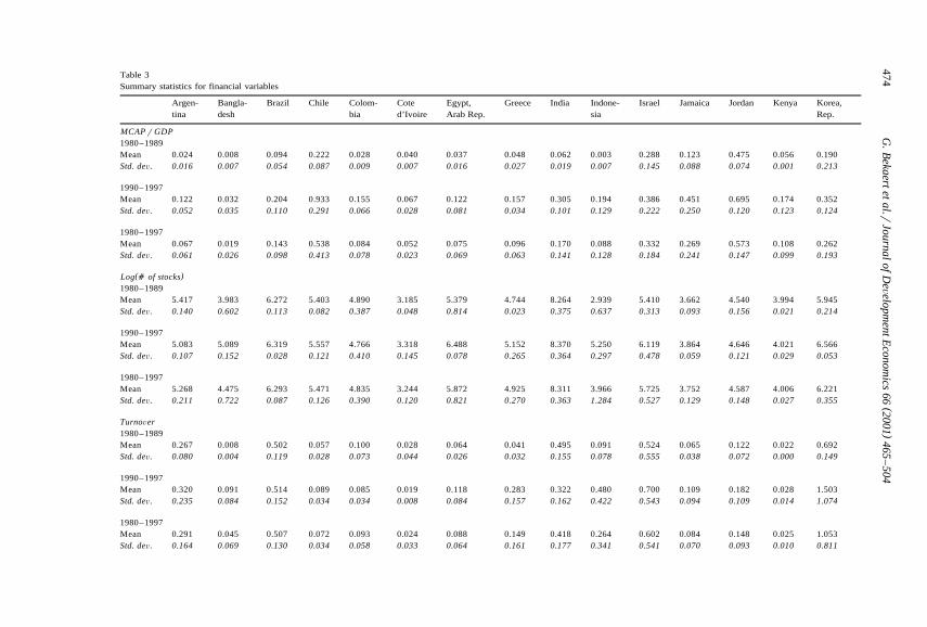
The focus of this paper is on the relation between economic growth and equitymarket liberalization. We examine three variables to proxy for the more generaldevelopment of the equity market: a measure of equity market size, the log of thenumber of domestic companies, and equity market turnover as a measure of
Ž . Ž .market liquidity. Both Bekaert and Harvey 1997 and Levine and Zervos 1998use the ratio of the equity market capitalization to gross domestic product as ameasure of the size of the local equity market. Large markets relative to the size ofthe economy in which they reside potentially indicate market development.
Ž .Bekaert and Harvey 2000 employ the log of the number of companies as aŽ .measure of market development. Atje and Jovanovic 1993 and Levine and
Ž .Zervos 1998 provide evidence for a strong relationship between economicgrowth and stock market liquidity, and, therefore, we employ value traded dividedby market capitalization in this capacity.
2.1. Summary statistics
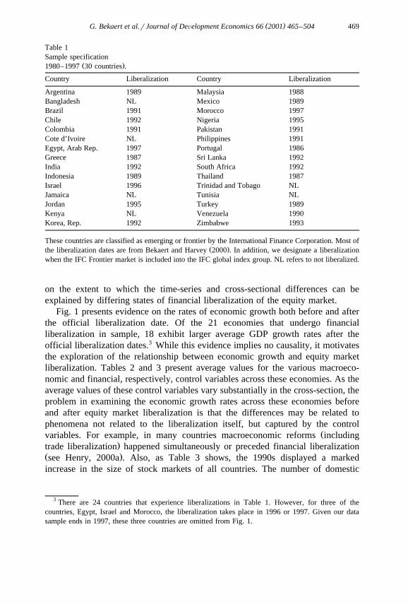
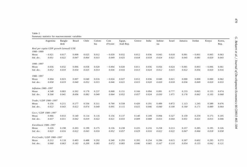
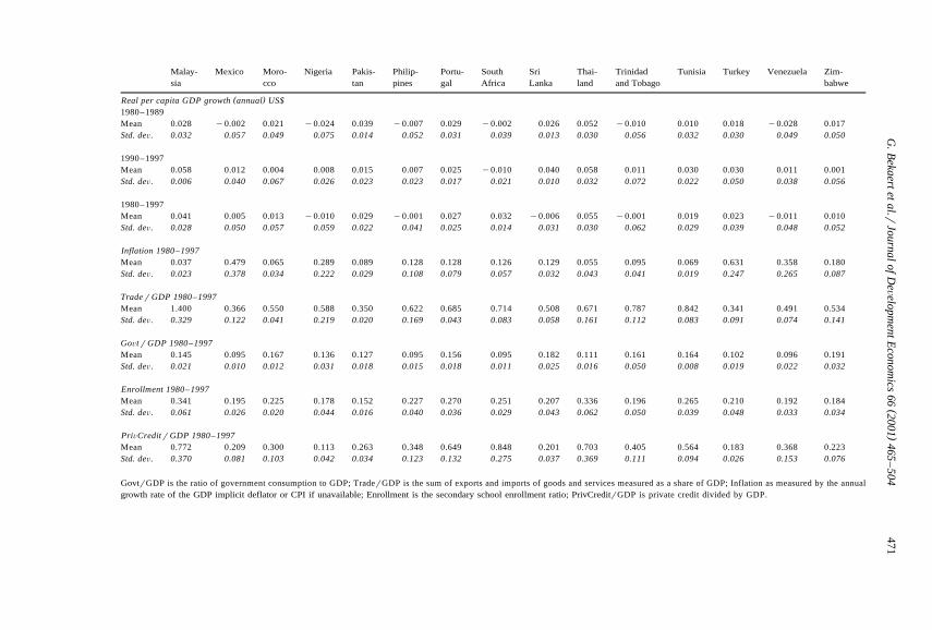
Table 1 describes the sample of 30 countries that we employ in estimation,classified as either emerging or frontier by the International Finance CorporationŽ .IFC, 1997 , for which there are annual data extending from 1980 to 1997. Table 2presents the summary statistics for the macro economic variables. This includesaverage real per capita GDP growth rates across the 30 countries in our sampleacross two decades. For this variable, we provide means over the 1980s and1990s, as well as for the full sample. The average growth rates differ substantiallyacross time for many of the economies considered. Additionally, the rates ofeconomic growth vary widely across the economies included. This paper focuses
( )G. Bekaert et al.rJournal of DeÕelopment Economics 66 2001 465–504 469
Table 1Sample specification
Ž .1980–1997 30 countries .
Country Liberalization Country Liberalization
Argentina 1989 Malaysia 1988Bangladesh NL Mexico 1989Brazil 1991 Morocco 1997Chile 1992 Nigeria 1995Colombia 1991 Pakistan 1991Cote d’Ivoire NL Philippines 1991Egypt, Arab Rep. 1997 Portugal 1986Greece 1987 Sri Lanka 1992India 1992 South Africa 1992Indonesia 1989 Thailand 1987Israel 1996 Trinidad and Tobago NLJamaica NL Tunisia NLJordan 1995 Turkey 1989Kenya NL Venezuela 1990Korea, Rep. 1992 Zimbabwe 1993
These countries are classified as emerging or frontier by the International Finance Corporation. Most ofŽ .the liberalization dates are from Bekaert and Harvey 2000 . In addition, we designate a liberalization
when the IFC Frontier market is included into the IFC global index group. NL refers to not liberalized.
on the extent to which the time-series and cross-sectional differences can beexplained by differing states of financial liberalization of the equity market.
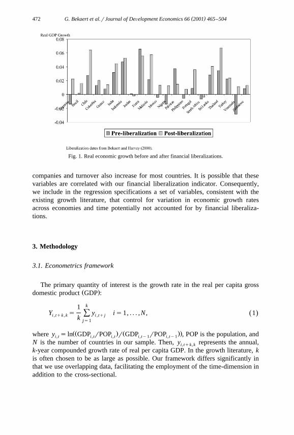
Fig. 1 presents evidence on the rates of economic growth both before and afterthe official liberalization date. Of the 21 economies that undergo financialliberalization in sample, 18 exhibit larger average GDP growth rates after theofficial liberalization dates.3 While this evidence implies no causality, it motivatesthe exploration of the relationship between economic growth and equity marketliberalization. Tables 2 and 3 present average values for the various macroeco-nomic and financial, respectively, control variables across these economies. As theaverage values of these control variables vary substantially in the cross-section, theproblem in examining the economic growth rates across these economies beforeand after equity market liberalization is that the differences may be related tophenomena not related to the liberalization itself, but captured by the control
Žvariables. For example, in many countries macroeconomic reforms including.trade liberalization happened simultaneously or preceded financial liberalization
Ž .see Henry, 2000a . Also, as Table 3 shows, the 1990s displayed a markedincrease in the size of stock markets of all countries. The number of domestic
3 There are 24 countries that experience liberalizations in Table 1. However, for three of thecountries, Egypt, Israel and Morocco, the liberalization takes place in 1996 or 1997. Given our datasample ends in 1997, these three countries are omitted from Fig. 1.
()
G.B
ekaertetal.r
JournalofD
eÕelopm
entEconom
ics66
2001465
–504
470
Table 2Summary statistics for macroeconomic variables
Argentina Bangla- Brazil Chile Colom- Cote Egypt, Greece India Indone- Israel Jamaica Jordan Kenya Korea,desh bia d’Ivoire Arab Rep. sia Rep.
( )Real per capita GDP growth annual US$1980–1989Mean y0.021 0.017 0.008 0.025 0.012 y0.039 0.032 0.012 0.036 0.043 0.018 0.001 y0.001 0.005 0.063Std. deÕ. 0.051 0.022 0.047 0.064 0.015 0.049 0.025 0.018 0.018 0.024 0.021 0.045 0.081 0.020 0.043
1990–1997Mean 0.036 0.032 0.006 0.058 0.020 y0.004 0.020 0.011 0.036 0.056 0.024 y0.001 0.003 y0.006 0.061Std. deÕ. 0.052 0.010 0.034 0.025 0.014 0.036 0.016 0.013 0.024 0.012 0.015 0.022 0.056 0.020 0.016
1980–1997Mean 0.004 0.023 0.007 0.040 0.016 y0.024 0.027 0.012 0.036 0.049 0.021 0.000 0.000 0.000 0.062Std. deÕ. 0.058 0.019 0.040 0.052 0.015 0.046 0.021 0.015 0.020 0.020 0.018 0.036 0.069 0.020 0.033
Inflation 1980–1997Mean 4.548 0.083 6.502 0.179 0.237 0.068 0.151 0.166 0.094 0.091 0.777 0.233 0.065 0.155 0.074Std. deÕ. 8.506 0.041 8.696 0.082 0.040 0.064 0.052 0.057 0.024 0.030 1.071 0.176 0.062 0.105 0.068
TraderGDP 1980–1997Mean 0.156 0.211 0.177 0.556 0.311 0.700 0.558 0.420 0.191 0.499 0.872 1.113 1.245 0.589 0.676Std. deÕ. 0.022 0.043 0.022 0.074 0.040 0.095 0.115 0.025 0.046 0.040 0.100 0.160 0.171 0.089 0.064
GoÕtrGDP 1980–1997Mean 0.066 0.033 0.140 0.114 0.116 0.156 0.137 0.140 0.109 0.094 0.327 0.159 0.259 0.173 0.105Std. deÕ. 0.037 0.011 0.042 0.019 0.022 0.021 0.033 0.009 0.008 0.015 0.044 0.031 0.021 0.015 0.006
Enrollment 1980–1997Mean 0.226 0.198 0.203 0.199 0.175 0.136 0.238 0.225 0.216 0.258 0.213 0.257 0.285 0.195 0.326Std. deÕ. 0.023 0.016 0.022 0.043 0.016 0.052 0.057 0.029 0.016 0.022 0.022 0.067 0.066 0.018 0.038
PriÕCreditrGDP 1980–1997Mean 0.212 0.118 0.493 0.488 0.292 0.340 0.293 0.395 0.254 0.296 0.615 0.307 0.602 0.295 0.572Std. deÕ. 0.068 0.063 0.183 0.209 0.085 0.072 0.083 0.046 0.065 0.167 0.110 0.054 0.155 0.042 0.121
()
G.B
ekaertetal.r
JournalofD
eÕelopm
entEconom
ics66
2001465
–504
471
Malay- Mexico Moro- Nigeria Pakis- Philip- Portu- South Sri Thai- Trinidad Tunisia Turkey Venezuela Zim-sia cco tan pines gal Africa Lanka land and Tobago babwe
( )Real per capita GDP growth annual US$1980–1989Mean 0.028 y0.002 0.021 y0.024 0.039 y0.007 0.029 y0.002 0.026 0.052 y0.010 0.010 0.018 y0.028 0.017Std. deÕ. 0.032 0.057 0.049 0.075 0.014 0.052 0.031 0.039 0.013 0.030 0.056 0.032 0.030 0.049 0.050
1990–1997Mean 0.058 0.012 0.004 0.008 0.015 0.007 0.025 y0.010 0.040 0.058 0.011 0.030 0.030 0.011 0.001Std. deÕ. 0.006 0.040 0.067 0.026 0.023 0.023 0.017 0.021 0.010 0.032 0.072 0.022 0.050 0.038 0.056
1980–1997Mean 0.041 0.005 0.013 y0.010 0.029 y0.001 0.027 0.032 y0.006 0.055 y0.001 0.019 0.023 y0.011 0.010Std. deÕ. 0.028 0.050 0.057 0.059 0.022 0.041 0.025 0.014 0.031 0.030 0.062 0.029 0.039 0.048 0.052
Inflation 1980–1997Mean 0.037 0.479 0.065 0.289 0.089 0.128 0.128 0.126 0.129 0.055 0.095 0.069 0.631 0.358 0.180Std. deÕ. 0.023 0.378 0.034 0.222 0.029 0.108 0.079 0.057 0.032 0.043 0.041 0.019 0.247 0.265 0.087
TraderGDP 1980–1997Mean 1.400 0.366 0.550 0.588 0.350 0.622 0.685 0.714 0.508 0.671 0.787 0.842 0.341 0.491 0.534Std. deÕ. 0.329 0.122 0.041 0.219 0.020 0.169 0.043 0.083 0.058 0.161 0.112 0.083 0.091 0.074 0.141
GoÕtrGDP 1980–1997Mean 0.145 0.095 0.167 0.136 0.127 0.095 0.156 0.095 0.182 0.111 0.161 0.164 0.102 0.096 0.191Std. deÕ. 0.021 0.010 0.012 0.031 0.018 0.015 0.018 0.011 0.025 0.016 0.050 0.008 0.019 0.022 0.032
Enrollment 1980–1997Mean 0.341 0.195 0.225 0.178 0.152 0.227 0.270 0.251 0.207 0.336 0.196 0.265 0.210 0.192 0.184Std. deÕ. 0.061 0.026 0.020 0.044 0.016 0.040 0.036 0.029 0.043 0.062 0.050 0.039 0.048 0.033 0.034
PriÕCreditrGDP 1980–1997Mean 0.772 0.209 0.300 0.113 0.263 0.348 0.649 0.848 0.201 0.703 0.405 0.564 0.183 0.368 0.223Std. deÕ. 0.370 0.081 0.103 0.042 0.034 0.123 0.132 0.275 0.037 0.369 0.111 0.094 0.026 0.153 0.076
GovtrGDP is the ratio of government consumption to GDP; TraderGDP is the sum of exports and imports of goods and services measured as a share of GDP; Inflation as measured by the annualgrowth rate of the GDP implicit deflator or CPI if unavailable; Enrollment is the secondary school enrollment ratio; PrivCreditrGDP is private credit divided by GDP.
( )G. Bekaert et al.rJournal of DeÕelopment Economics 66 2001 465–504472
Fig. 1. Real economic growth before and after financial liberalizations.
companies and turnover also increase for most countries. It is possible that thesevariables are correlated with our financial liberalization indicator. Consequently,we include in the regression specifications a set of variables, consistent with theexisting growth literature, that control for variation in economic growth ratesacross economies and time potentially not accounted for by financial liberaliza-tions.
3. Methodology
3.1. Econometrics framework
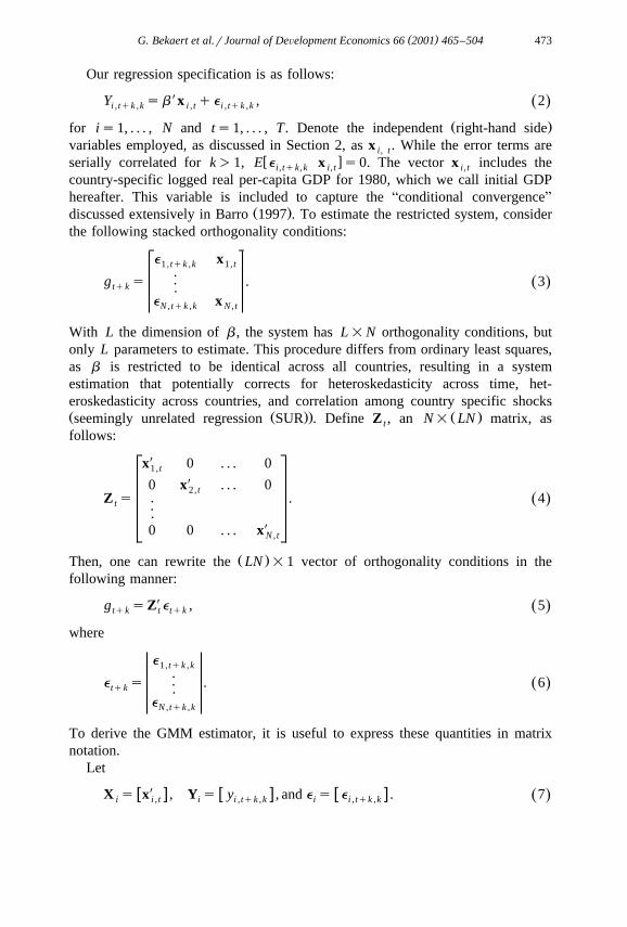
The primary quantity of interest is the growth rate in the real per capita grossŽ .domestic product GDP :
k1Y s y is1, . . . , N , 1Ž .Ýi , tqk ,k i , tqjk js1
ŽŽ . Ž ..where y s ln GDP rPOP r GDP rPOP , POP is the population, andi, t i, t i, t i, ty1 i, ty1
N is the number of countries in our sample. Then, y represents the annual,i, tqk ,k
k-year compounded growth rate of real per capita GDP. In the growth literature, kis often chosen to be as large as possible. Our framework differs significantly inthat we use overlapping data, facilitating the employment of the time-dimension inaddition to the cross-sectional.
( )G. Bekaert et al.rJournal of DeÕelopment Economics 66 2001 465–504 473
Our regression specification is as follows:
Y sbXx qe , 2Ž .i , tqk ,k i , t i , tqk ,k
Ž .for is1, . . . , N and ts1, . . . , T. Denote the independent right-hand sidevariables employed, as discussed in Section 2, as x . While the error terms arei, t
w xserially correlated for k)1, E e x s0. The vector x includes thei, tqk ,k i, t i, t
country-specific logged real per-capita GDP for 1980, which we call initial GDPhereafter. This variable is included to capture the Aconditional convergenceB
Ž .discussed extensively in Barro 1997 . To estimate the restricted system, considerthe following stacked orthogonality conditions:
e x1, tqk ,k 1, t..g s . 3Ž .tqk .
e xN , tqk ,k N , t
With L the dimension of b , the system has L=N orthogonality conditions, butonly L parameters to estimate. This procedure differs from ordinary least squares,as b is restricted to be identical across all countries, resulting in a systemestimation that potentially corrects for heteroskedasticity across time, het-eroskedasticity across countries, and correlation among country specific shocksŽ Ž .. Ž .seemingly unrelated regression SUR . Define Z , an N= LN matrix, ast
follows:
Xx 0 . . . 01, tX0 x . . . 02, t
.Z s . 4Ž .t ..X0 0 . . . x N , t
Ž .Then, one can rewrite the LN =1 vector of orthogonality conditions in thefollowing manner:
g sZXe , 5Ž .tqk t tqk
where
e1, tqk ,k..e s . 6Ž .tqk .
eN , tqk ,k
To derive the GMM estimator, it is useful to express these quantities in matrixnotation.
Let
w X x w x w xX s x , Y s y , and e s e . 7Ž .i i , t i i , tqk ,k i i , tqk ,k
()
G.B
ekaertetal.r
JournalofD
eÕelopm
entEconom
ics66
2001465
–504
474Table 3Summary statistics for financial variables
Argen- Bangla- Brazil Chile Colom- Cote Egypt, Greece India Indone- Israel Jamaica Jordan Kenya Korea,tina desh bia d’Ivoire Arab Rep. sia Rep.
MCAPrGDP1980–1989Mean 0.024 0.008 0.094 0.222 0.028 0.040 0.037 0.048 0.062 0.003 0.288 0.123 0.475 0.056 0.190Std. deÕ. 0.016 0.007 0.054 0.087 0.009 0.007 0.016 0.027 0.019 0.007 0.145 0.088 0.074 0.001 0.213
1990–1997Mean 0.122 0.032 0.204 0.933 0.155 0.067 0.122 0.157 0.305 0.194 0.386 0.451 0.695 0.174 0.352Std. deÕ. 0.052 0.035 0.110 0.291 0.066 0.028 0.081 0.034 0.101 0.129 0.222 0.250 0.120 0.123 0.124
1980–1997Mean 0.067 0.019 0.143 0.538 0.084 0.052 0.075 0.096 0.170 0.088 0.332 0.269 0.573 0.108 0.262Std. deÕ. 0.061 0.026 0.098 0.413 0.078 0.023 0.069 0.063 0.141 0.128 0.184 0.241 0.147 0.099 0.193
( )Log a of stocks1980–1989Mean 5.417 3.983 6.272 5.403 4.890 3.185 5.379 4.744 8.264 2.939 5.410 3.662 4.540 3.994 5.945Std. deÕ. 0.140 0.602 0.113 0.082 0.387 0.048 0.814 0.023 0.375 0.637 0.313 0.093 0.156 0.021 0.214
1990–1997Mean 5.083 5.089 6.319 5.557 4.766 3.318 6.488 5.152 8.370 5.250 6.119 3.864 4.646 4.021 6.566Std. deÕ. 0.107 0.152 0.028 0.121 0.410 0.145 0.078 0.265 0.364 0.297 0.478 0.059 0.121 0.029 0.053
1980–1997Mean 5.268 4.475 6.293 5.471 4.835 3.244 5.872 4.925 8.311 3.966 5.725 3.752 4.587 4.006 6.221Std. deÕ. 0.211 0.722 0.087 0.126 0.390 0.120 0.821 0.270 0.363 1.284 0.527 0.129 0.148 0.027 0.355
TurnoÕer1980–1989Mean 0.267 0.008 0.502 0.057 0.100 0.028 0.064 0.041 0.495 0.091 0.524 0.065 0.122 0.022 0.692Std. deÕ. 0.080 0.004 0.119 0.028 0.073 0.044 0.026 0.032 0.155 0.078 0.555 0.038 0.072 0.000 0.149
1990–1997Mean 0.320 0.091 0.514 0.089 0.085 0.019 0.118 0.283 0.322 0.480 0.700 0.109 0.182 0.028 1.503Std. deÕ. 0.235 0.084 0.152 0.034 0.034 0.008 0.084 0.157 0.162 0.422 0.543 0.094 0.109 0.014 1.074
1980–1997Mean 0.291 0.045 0.507 0.072 0.093 0.024 0.088 0.149 0.418 0.264 0.602 0.084 0.148 0.025 1.053Std. deÕ. 0.164 0.069 0.130 0.034 0.058 0.033 0.064 0.161 0.177 0.341 0.541 0.070 0.093 0.010 0.811

()
G.B
ekaertetal.r
JournalofD
eÕelopm
entEconom
ics66
2001465
–504
475
Malay- Mexico Morocco Nigeria Pakistan Philip- Portugal South Sri Thailand Trinidad Tunisia Turkey Vene- Zim-sia pines Africa Lanka and Tobago zuela babwe
MCAPrGDP1980–1989Mean 0.634 0.044 0.021 0.060 0.045 0.085 0.063 0.065 1.208 0.090 0.113 0.067 0.020 0.032 0.100Std. deÕ. 0.166 0.030 0.003 0.028 0.014 0.076 0.087 0.009 0.301 0.100 0.044 0.003 0.017 0.008 0.070
1990–1997Mean 2.096 0.332 0.148 0.073 0.169 0.547 0.184 0.174 1.599 0.583 0.198 0.117 0.159 0.133 0.243Std. deÕ. 0.971 0.105 0.110 0.028 0.050 0.331 0.089 0.052 0.400 0.319 0.144 0.074 0.079 0.053 0.098
1980–1997Mean 1.284 0.172 0.077 0.066 0.100 0.290 0.117 0.113 1.382 0.309 0.151 0.089 0.082 0.077 0.164Std. deÕ. 0.981 0.164 0.096 0.028 0.072 0.322 0.105 0.065 0.392 0.333 0.107 0.054 0.088 0.062 0.109
( )Log a of stocks1980–1989Mean 5.366 5.246 4.322 4.573 5.872 5.080 3.860 5.146 6.318 4.629 3.491 2.565 4.821 4.548 4.041Std. deÕ. 0.107 0.175 0.034 0.062 0.113 0.184 0.909 0.014 0.240 0.270 0.078 0.000 1.057 0.278 0.070
1990–1997Mean 6.097 5.282 4.037 5.101 6.494 5.222 5.164 5.327 6.494 5.842 3.283 3.017 5.134 4.477 4.128Std. deÕ. 0.320 0.040 0.172 0.130 0.178 0.136 0.095 0.123 0.053 0.258 0.090 0.361 0.288 0.063 0.042
1980–1997Mean 5.691 5.262 4.195 4.808 6.149 5.143 4.440 5.226 6.396 5.168 3.398 2.766 4.960 4.517 4.080Std. deÕ. 0.434 0.132 0.185 0.286 0.348 0.176 0.942 0.122 0.200 0.671 0.134 0.327 0.807 0.209 0.073
TurnoÕer1980–1989Mean 0.151 0.629 0.044 0.006 0.123 0.221 0.066 0.012 0.048 0.384 0.095 0.050 0.031 0.043 0.077Std. deÕ. 0.051 0.482 0.019 0.003 0.037 0.132 0.073 0.006 0.011 0.222 0.053 0.000 0.039 0.032 0.063
1990–1997Mean 0.556 0.386 0.131 0.013 0.334 0.274 0.328 0.113 0.087 0.768 0.085 0.080 0.996 0.237 0.082Std. deÕ. 0.456 0.107 0.128 0.011 0.332 0.153 0.109 0.067 0.047 0.288 0.032 0.050 0.664 0.074 0.080
1980–1997Mean 0.331 0.521 0.083 0.009 0.217 0.245 0.183 0.057 0.065 0.554 0.090 0.063 0.460 0.129 0.079Std. deÕ. 0.360 0.378 0.094 0.008 0.240 0.140 0.160 0.067 0.037 0.314 0.044 0.035 0.653 0.112 0.069
Ž .MCAPrGDP is equity market capitalization of the IFC index divided by GDP; log a of stocks is the log of the number of domestic companies in the IFC index; Turnover is the ratio of equitymarket value traded to the MCAP for the IFC index.

( )G. Bekaert et al.rJournal of DeÕelopment Economics 66 2001 465–504476
Also,
X Y e1 1 1. . .. . .Xs , Ys , and es , 8Ž .. . .eX Y NN N
where X is a TN=L matrix and Y and e are TN=1 matrices. Also, let
X 0 . . . 01
0 X . . . 02.Zs , 9Ž ...0 0 . . . X N
a TN=LN matrix. It follows,
esYyXb . 10Ž .Additionally,
T1g s gÝT tqkT ts1
1Xs Z YyXb . 11� 4Ž . Ž .
T
Employing this notation, the GMM estimator satisfies
X y1bsarg min g S g , 12Ž .T T Tb
Ž .where S is the inverse of the GMM weighting matrix see below . The FirstT
Order Condition associated with this optimum is as follows:
EgXT y1S g s0. 13Ž .T T
Eb
Note that
Eg ZXXTs . 14Ž .
Eb T
Hence, to set the first order condition to zero, we choose
y1X X X Xy1 y1bs X Z S Z X X Z S Z Y . 15Ž . Ž . Ž . Ž . Ž .T T
This is a well-known result from IV-estimators in a GMM framework. Weoptimally choose the GMM weighting matrix to minimize the variance–covariance

( )G. Bekaert et al.rJournal of DeÕelopment Economics 66 2001 465–504 477
matrix of the estimated parameter vector; S is the estimated variance covarianceT1
TŽ .matrix of Ý g , taking all possible autocovariances into account:ts1 tT`
Xw xS s E g g . 16Ž .ÝT tqk tqkyjjsy`
Using the identity matrix as the weighting matrix, first step parameter estimatesare obtained as follows:
y1X X X Xb s X Z Z X X Z Z Y . 17Ž . Ž . Ž . Ž . Ž .1
Then, construct the first step residuals as follows:
ˆesYyXb . 18Ž .ˆ 1
For the second step estimation, we use e to construct the optimal weightingˆˆy1 Ž .matrix S . In the case of overlapping data k)1 , the residuals follow anT
Ž .MA ky1 process. This structure allows the consideration of four differentspecifications for the weighting matrix that facilitate increasingly restricted vari-
Ž .ance–covariance structures across the residuals in Eq. 2 .
3.1.1. Weighting matrix IThe most general specification facilitates temporal heteroskedasticity, cross-sec-
tional heteroskedasticity, and SUR effects.
1X XS s Z e e ZÝT t tqk tqk tT t
K TjX X X Xq 1y Z e e Z qZ e e Z .Ž .Ý Ý ty j tqkyj tqk t t tqk tqkyj tyjž /Kq1js1 tsjq1
19Ž .
In order to ensure that the variance–covariance matrix is positive-definite, theŽ . Ž .Newey and West 1987 estimator is employed. K )k is chosen to be 9, which
is large enough to sufficiently capture the longer lagged effects and to ensureconsistency. As the time dimension in our sample, T , is small, we do not considerthis weighting matrix specification in practice. In the interest of parsimony, weconsider three restricted variance–covariance structures.
3.1.2. Weighting matrix IIThis specification facilitates cross-sectional heteroskedasticity and SUR effects,
ˆbut not temporal heteroskedasticity. Define the N=N matrix V as follows:j
T1XV s e e . 20Ž . Ž .Ýj tqk tqkyjT tsjq1
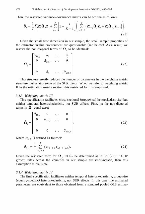
( )G. Bekaert et al.rJournal of DeÕelopment Economics 66 2001 465–504478
Then, the restricted variance–covariance matrix can be written as follows:
K T1 jX X Xˆ ˆ ˆ ˆS s Z V Z q 1y Z V Z qZ V Z .Ý Ý Ý ž /T t 0 t tyj j t t yj tyjž /T Kq1t js1 tsjq1
21Ž .
Given the small time dimension in our sample, the small sample properties ofŽ .the estimator in this environment are questionable see below . As a result, we
ˆrestrict the non-diagonal terms of V to be identical:j
s s . . . sˆ ˆ ˆ11 , j j j
s s . . . sˆ ˆ ˆj 22, j jV s . 22. Ž .j ..
s s . . . sˆ ˆ ˆj j NN , j
This structure greatly reduces the number of parameters in the weighting matrixstructure, but retains some of the SUR flavor. When we refer to weighting matrixII in the estimation results section, this restricted form is employed.
3.1.3. Weighting matrix IIIŽ .This specification facilitates cross-sectional groupwise heteroskedasticity, but
neither temporal heteroskedasticity nor SUR effects. First, let the non-diagonalˆterms in V equal zero:j
s 0 . . . 0ˆ11 , j
0 s . . . 0ˆ22 , jV s , 23. Ž .j ..
0 0 . . . sNN , j
where s is defined as follows:i i, j
T1X
s s e e . 24Ž . Ž .ˆ Ýi i , j i , tqk ,k i , tqkyj ,kT tsjq1
ˆ ˆ Ž .Given the restricted form for V , let S be determined as in Eq. 21 . If GDPj T
growth rates across the countries in our sample are idiosyncratic, then thisassumption is plausible.
3.1.4. Weighting matrix IVThe final specification facilitates neither temporal heteroskedasticity, groupwise
Ž .country-specific heteroskedasticity, nor SUR effects. In this case, the estimatedparameters are equivalent to those obtained from a standard pooled OLS estima-
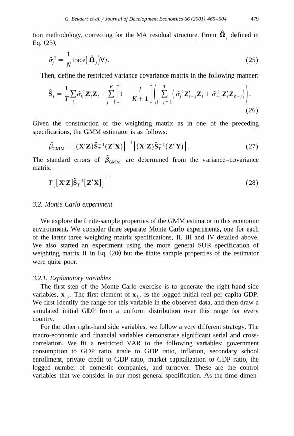
( )G. Bekaert et al.rJournal of DeÕelopment Economics 66 2001 465–504 479
ˆtion methodology, correcting for the MA residual structure. From V defined injŽ .Eq. 23 ,
12 ˆs s trace V ; j. 25Ž .ˆ ž /j jN
Then, define the restricted variance covariance matrix in the following manner:
K T1 jX X X2 2 2S s s Z Z q 1y s Z Z qs Z Z .ˆ ˆ ˆÝ Ý Ý ž /T 0 t t j tyj t yj t tyjž /T Kq1t js1 tsjq1
26Ž .
Given the construction of the weighting matrix as in one of the precedingspecifications, the GMM estimator is as follows:
y1X X X Xy1 y1ˆ ˆ ˆb s X Z S Z X X Z S Z Y . 27Ž . Ž . Ž . Ž . Ž .GMM T T
ˆThe standard errors of b are determined from the variance–covarianceGMM
matrix:
y1X Xy1ˆw x w xT X Z S Z X 28Ž .T
3.2. Monte Carlo experiment
We explore the finite-sample properties of the GMM estimator in this economicenvironment. We consider three separate Monte Carlo experiments, one for eachof the latter three weighting matrix specifications, II, III and IV detailed above.We also started an experiment using the more general SUR specification of
Ž .weighting matrix II in Eq. 20 but the finite sample properties of the estimatorwere quite poor.
3.2.1. Explanatory ÕariablesThe first step of the Monte Carlo exercise is to generate the right-hand side
variables, x . The first element of x is the logged initial real per capita GDP.i, t i, t
We first identify the range for this variable in the observed data, and then draw asimulated initial GDP from a uniform distribution over this range for everycountry.
For the other right-hand side variables, we follow a very different strategy. Themacro-economic and financial variables demonstrate significant serial and cross-correlation. We fit a restricted VAR to the following variables: governmentconsumption to GDP ratio, trade to GDP ratio, inflation, secondary schoolenrollment, private credit to GDP ratio, market capitalization to GDP ratio, thelogged number of domestic companies, and turnover. These are the controlvariables that we consider in our most general specification. As the time dimen-

( )G. Bekaert et al.rJournal of DeÕelopment Economics 66 2001 465–504480
sion, T , is small in our sample, we restrict the VAR coefficients to be identicalacross countries, but we allow for country specific intercepts. The restrictedcoefficient matrix, reported in the table in Appendix B, is estimated using pooled
Ž .OLS we also report the standard errors of the restricted VAR . Given therestricted VAR coefficients, for each country we begin the variables at theirunconditional means from the observed data. We simulate 100qT values fromthe VAR for each country, and discard the initial 100 simulated observations.Now, we have simulated observations for the right-hand side variables, x ,i, t
excluding the official liberalization indicator, to which we turn below.
3.2.2. The dependent ÕariableThe real per capita GDP growth is determined according to the model as a
function of the right-hand side variables, x and the residuals, e . The null model isas follows:
y sbXx qe , 29Ž .˜ ˜ ˜i , tqk ,k i , t i , tqk ,k
with no official liberalization indicator included in the right-hand side variables.The b-vector comes from our growth model specification prior to introducing theindicator variables presented in Table 7. As there are three separate Monte Carlodesigns, that is, one for each of the three weighting matrices under consideration,b is chosen from Table 7 for each of the three to reflect the particular weightingmatrix under consideration. Given the use of overlapping data, the residuals follow
Ž .an MA ky1 process. To mimic this environment, we estimate a restrictedŽ .MA ky1 model for each of the residuals from the estimations performed in
Table 7, depending upon the length k. The restriction lies in the fact that weŽ .jointly estimate the MA ky1 process for each country, restricting the MA
coefficients to be identical across countries. This restriction is motivated inprecisely the same way the VAR’s are restricted given the limited time seriesdimension. The restricted MA coefficients, reported in the table in Appendix B for
Ž .ks2, . . . , 5, are estimated using quasi-maximum likelihood QMLE whichassumes uncorrelated errors across countries and normal shocks in the likelihoodfunction. Then, we construct the simulated residuals as follows:
ky1
e ss u u , 30Ž .˜ Ýi , tqk ,k i j tqkyj , iž /js0
where the u are drawn from a standard normal distribution, s is thetqky j, i iŽestimated standard deviation for country i given as the sample standard deviation
.of the residuals from the regressions reported in Table 7 , and the u are thej
cross-sectionally restricted MA coefficients, where u s1.4 Notice that the error0
terms are independent of the right-hand side control variables.
4 One extension is to allow the errors to be correlated. This would better reflect the SUR estimationstructure, whereas the groupwise heteroskedasticity estimation structure is related to s .i
( )G. Bekaert et al.rJournal of DeÕelopment Economics 66 2001 465–504 481
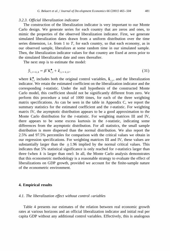
3.2.3. Official liberalization indicatorThe construction of the liberalization indicator is very important to our Monte
Carlo design. We generate series for each country that are zeros and ones, tomimic the properties of the observed liberalization indicator. First, we generatesimulated liberalization dates drawn from a uniform distribution over the timeseries dimension, i.e. from 1 to T , for each country, so that each economy, as inour observed sample, liberalizes at some random time in our simulated sample.Then, the liberalization indicator values for that country are fixed at zeros prior tothe simulated liberalization date and ones thereafter.
The next step is to estimate the model:
y sbXxw qe , 31Ž .˜ ˜ ˜i , tqk ,k i , t i , tqk ,k
where xw includes both the original control variables, x , and the liberalization˜ ˜i, t i, t
indicator. We retain the estimated coefficient on the liberalization indicator and thecorresponding t-statistic. Under the null hypothesis of the constructed MonteCarlo model, this coefficient should not be significantly different from zero. Weperform this procedure a total of 1000 times, for each of the three weightingmatrix specifications. As can be seen in the table in Appendix C, we report thesummary statistics for the estimated coefficient and the t-statistic. For weightingmatrix IV, the asymptotic distribution appears to be a good approximation to theMonte Carlo distribution for the t-statistic. For weighting matrices III and IV,there appears to be some excess kurtosis in the t-statistic, indicating somedifferences from the asymptotic distribution. For all statistics, the small sampledistribution is more dispersed than the normal distribution. We also report the2.5% and 97.5% percentiles for comparison with the critical values we obtain inour regression specifications. For weighting matrices III and IV, these values aresubstantially larger than the "1.96 implied by the normal critical values. Thisindicates that 5% statistical significance is only reached for t-statistics larger than
Ž .three when k is larger than one . In all, the Monte Carlo analysis demonstratesthat this econometric methodology is a reasonable strategy to evaluate the effect ofliberalizations on GDP growth, provided we account for the finite-sample natureof the econometric environment.
4. Empirical results
4.1. The liberalization effect without control Õariables
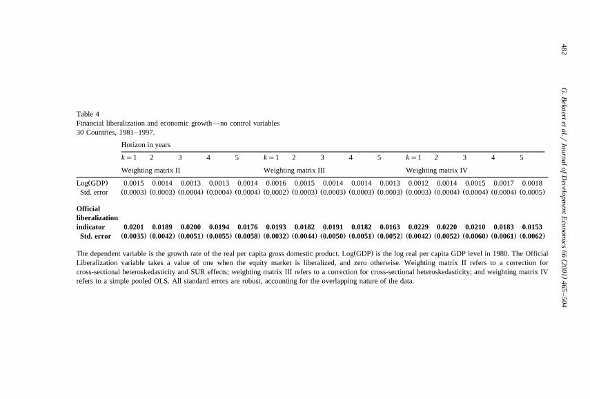
Table 4 presents our estimates of the relation between real economic growthrates at various horizons and an official liberalization indicator and initial real percapita GDP without any additional control variables. Effectively, this is analogous
()
G.B
ekaertetal.r
JournalofD
eÕelopm
entEconom
ics66
2001465
–504
482
Table 4Financial liberalization and economic growth—no control variables30 Countries, 1981–1997.
Horizon in years
ks1 2 3 4 5 ks1 2 3 4 5 ks1 2 3 4 5
Weighting matrix II Weighting matrix III Weighting matrix IV
Ž .Log GDP 0.0015 0.0014 0.0013 0.0013 0.0014 0.0016 0.0015 0.0014 0.0014 0.0013 0.0012 0.0014 0.0015 0.0017 0.0018Ž . Ž . Ž . Ž . Ž . Ž . Ž . Ž . Ž . Ž . Ž . Ž . Ž . Ž . Ž .Std. error 0.0003 0.0003 0.0004 0.0004 0.0004 0.0002 0.0003 0.0003 0.0003 0.0003 0.0003 0.0004 0.0004 0.0004 0.0005
Officialliberalizationindicator 0.0201 0.0189 0.0200 0.0194 0.0176 0.0193 0.0182 0.0191 0.0182 0.0163 0.0229 0.0220 0.0210 0.0183 0.0153
Ž . Ž . Ž . Ž . Ž . Ž . Ž . Ž . Ž . Ž . Ž . Ž . Ž . Ž . Ž .Std. error 0.0035 0.0042 0.0051 0.0055 0.0058 0.0032 0.0044 0.0050 0.0051 0.0052 0.0042 0.0052 0.0060 0.0061 0.0062
Ž .The dependent variable is the growth rate of the real per capita gross domestic product. Log GDP is the log real per capita GDP level in 1980. The OfficialLiberalization variable takes a value of one when the equity market is liberalized, and zero otherwise. Weighting matrix II refers to a correction forcross-sectional heteroskedasticity and SUR effects; weighting matrix III refers to a correction for cross-sectional heteroskedasticity; and weighting matrix IVrefers to a simple pooled OLS. All standard errors are robust, accounting for the overlapping nature of the data.
( )G. Bekaert et al.rJournal of DeÕelopment Economics 66 2001 465–504 483
to exploring the mean growth rate before and after financial liberalization.Consistent with the evidence on the pre and post-liberalization average growthrates presented in Section 2, these estimates demonstrate a positive and statisticallysignificant relation between financial liberalization and economic growth across avariety of specifications and horizons.
In each case, the estimated coefficient is presented when the GMM weightingmatrix is constructed as in either specification II, III or IV in the previous section.Specification II is the most general that we consider in that it allows for
Ž .cross-sectional heteroskedasticity and restricted SUR effects, whereas the lattertwo are more restricted versions. Regardless of weighting matrix specification, theestimated coefficient is positive and significant in all cases. The evidence impliesthat real GDP per capita growth rates increase following financial liberalization byanywhere from 1.5% to as large as 2.3% per annum, on average. For example,with a 3-year horizon using weighting matrix II, the impact on real economicgrowth rates is 2.0%. The evidence presented in Table 4 suggests that, on average,real economic growth rates increase roughly 1.9% per annum following financialliberalization.
Next, we present evidence on how this relation changes when additionalvariables are employed to control for various phenomena unrelated to the financialliberalization. Interestingly, the initial GDP appear to be positively related to thelevel of economic growth, in contrast to the convergence theory; however, muchlike the purely cross-sectional growth regressions, this relationship will changedramatically as additional control variables are added, lending credence to the
Ž . 5concept of Aconditional convergenceB presented in Barro 1997 .
4.2. Allowing for control Õariables
The shortcoming of exploring the changes in real economic growth rates beforeand after financial liberalization is that the observed change may be related tovarious economic and political phenomena unrelated to the financial liberalization.For example, periods of financial liberalization may be contemporaneous withperiods of political reform or economic restructuring. When estimating the relationbetween growth and financial liberalization, it is important to account for thesepotentially confounding effects. Consequently, we develop a hierarchical estima-tion strategy that evaluates the ability of incrementally increasing control groups toexplain the cross-sectional and time-series characteristics of real economic growth.
First, we begin by estimating the relation between economic growth rates andseveral macroeconomic variables that are commonly employed in the literature toexplain cross-sectional differences. Second, given the evidence presented in King
5 The control variables potentially capture the differing steady state per capita GDPs acrossŽ .countries, and convergence is defined relative to these differing steady states. See Barro 1997 .
( )G. Bekaert et al.rJournal of DeÕelopment Economics 66 2001 465–504484
Ž .and Levine 1993 , we then add control variables which represent bankingdevelopment. Third, we add equity market variables. These control variablesencompass many of the variables deemed important in explaining the cross-section
Ž .of economic growth rates in Atje and Jovanovic 1993 and Levine and ZervosŽ .1998 . Finally in Section 4.3, we add the official liberalization indicator, andreexamine the relation between financial liberalization and economic growthhaving controlled for unrelated effects using variables employed frequently in theliterature.
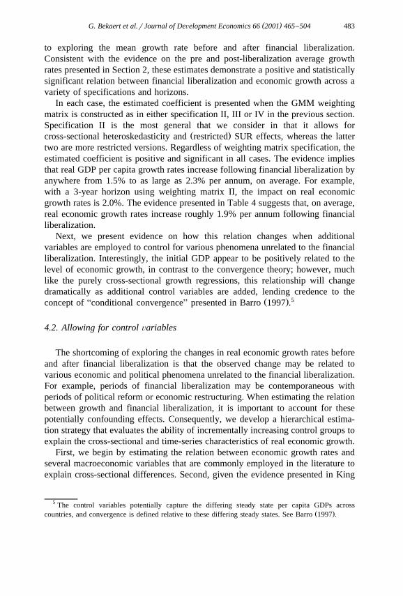
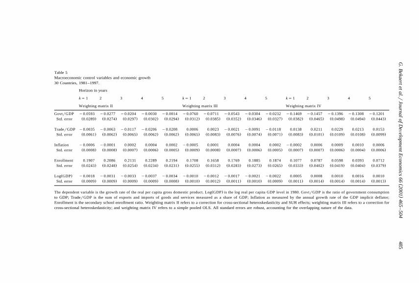
In accordance with our tiered strategy, the first set of regressions we considerinvolve the use of three macroeconomic conditioning variables and a humancapital variable: government consumption as a share of GDP, the size of the tradesector as a share of GDP, the annual inflation rate, and secondary schoolenrollment.
Table 5 presents evidence on the relation between these variables and economicgrowth. As before, we present the evidence obtained using the different GMMweighting matrix specifications. While the estimated relation between these vari-ables and real economic growth is not entirely consistent across samples andestimation specifications, several patterns do emerge. First, as in Barro and
Ž .Sala-i-Martin 1995 , high levels of government consumption are negativelyŽ .significantly related to economic growth rates, suggesting that the instabilities ortaxation associated with government consumption are obstacles to economicdevelopment. However, this relationship is statistically insignificant for weightingmatrix II. Second, the relation between the size of the trade sector and economicgrowth is statistically weak, and varies across the weighting matrix specifications
Ž . Ž .which is consistent with the results in Edwards 1998 and Rodrik 1999 . Therelation between inflation and economic growth generally is mostly statisticallyinsignificant and switches signs. Moreover, the measured effect is very small froman economic perspective. Additionally, secondary school enrollment is generallypositively and significantly related to economic growth across all weighting matrixspecifications. Finally, the relationship between initial GDP and economic growthis negative for weighting matrices II and III, indicating Aconditional convergenceBonce these additional control variables are included.
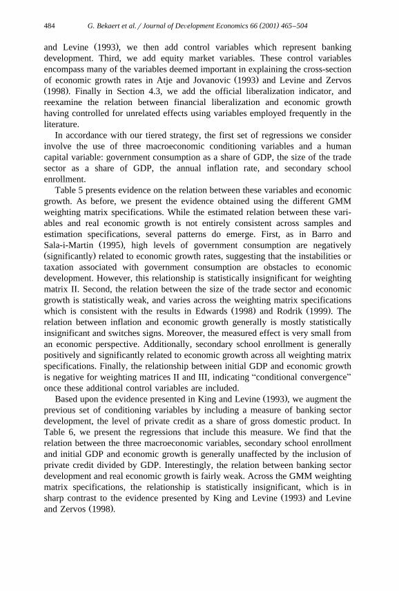
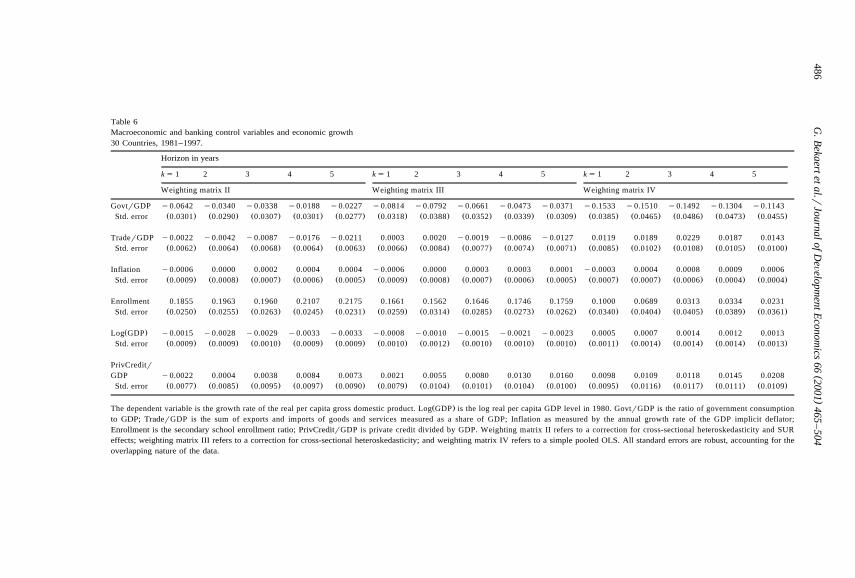
Ž .Based upon the evidence presented in King and Levine 1993 , we augment theprevious set of conditioning variables by including a measure of banking sectordevelopment, the level of private credit as a share of gross domestic product. InTable 6, we present the regressions that include this measure. We find that therelation between the three macroeconomic variables, secondary school enrollmentand initial GDP and economic growth is generally unaffected by the inclusion ofprivate credit divided by GDP. Interestingly, the relation between banking sectordevelopment and real economic growth is fairly weak. Across the GMM weightingmatrix specifications, the relationship is statistically insignificant, which is in
Ž .sharp contrast to the evidence presented by King and Levine 1993 and LevineŽ .and Zervos 1998 .
()
G.B
ekaertetal.r
JournalofD
eÕelopm
entEconom
ics66
2001465
–504
485
Table 5Macroeconomic control variables and economic growth30 Countries, 1981–1997.
Horizon in years
ks 1 2 3 4 5 ks 1 2 3 4 5 ks 1 2 3 4 5
Weighting matrix II Weighting matrix III Weighting matrix IV
GovtrGDP y0.0593 y0.0277 y0.0204 y0.0030 y0.0014 y0.0760 y0.0711 y0.0543 y0.0304 y0.0232 y0.1469 y0.1457 y0.1396 y0.1308 y0.1201Ž . Ž . Ž . Ž . Ž . Ž . Ž . Ž . Ž . Ž . Ž . Ž . Ž . Ž . Ž .Std. error 0.0289 0.0274 0.0297 0.0302 0.0294 0.0312 0.0385 0.0352 0.0346 0.0327 0.0382 0.0465 0.0498 0.0494 0.0443
TraderGDP y0.0035 y0.0063 y0.0117 y0.0206 y0.0208 0.0006 0.0023 y0.0021 y0.0091 y0.0118 0.0138 0.0211 0.0229 0.0213 0.0153Ž . Ž . Ž . Ž . Ž . Ž . Ž . Ž . Ž . Ž . Ž . Ž . Ž . Ž . Ž .Std. error 0.0061 0.0062 0.0065 0.0062 0.0062 0.0065 0.0083 0.0076 0.0074 0.0071 0.0083 0.0101 0.0109 0.0108 0.0099
Inflation y0.0006 y0.0001 0.0002 0.0004 0.0002 y0.0005 0.0001 0.0004 0.0004 0.0002 y0.0002 0.0006 0.0009 0.0010 0.0006Ž . Ž . Ž . Ž . Ž . Ž . Ž . Ž . Ž . Ž . Ž . Ž . Ž . Ž . Ž .Std. error 0.0008 0.0008 0.0007 0.0006 0.0005 0.0009 0.0008 0.0007 0.0006 0.0005 0.0007 0.0007 0.0006 0.0004 0.0006
Enrollment 0.1907 0.2086 0.2131 0.2289 0.2194 0.1708 0.1658 0.1769 0.1885 0.1874 0.1077 0.0787 0.0598 0.0393 0.0712Ž . Ž . Ž . Ž . Ž . Ž . Ž . Ž . Ž . Ž . Ž . Ž . Ž . Ž . Ž .Std. error 0.0243 0.0248 0.0254 0.0234 0.0231 0.0255 0.0312 0.0283 0.0273 0.0265 0.0333 0.0402 0.0419 0.0404 0.0379
Ž .Log GDP y0.0018 y0.0031 y0.0033 y0.0037 y0.0034 y0.0010 y0.0012 y0.0017 y0.0021 y0.0022 0.0005 0.0008 0.0010 0.0016 0.0010Ž . Ž . Ž . Ž . Ž . Ž . Ž . Ž . Ž . Ž . Ž . Ž . Ž . Ž . Ž .Std. error 0.0009 0.0009 0.0009 0.0009 0.0008 0.0010 0.0012 0.0011 0.0010 0.0009 0.0011 0.0014 0.0014 0.0014 0.0013
Ž .The dependent variable is the growth rate of the real per capita gross domestic product. Log GDP is the log real per capita GDP level in 1980. GovtrGDP is the ratio of government consumptionto GDP; TraderGDP is the sum of exports and imports of goods and services measured as a share of GDP; Inflation as measured by the annual growth rate of the GDP implicit deflator;Enrollment is the secondary school enrollment ratio. Weighting matrix II refers to a correction for cross-sectional heteroskedasticity and SUR effects; weighting matrix III refers to a correction forcross-sectional heteroskedasticity; and weighting matrix IV refers to a simple pooled OLS. All standard errors are robust, accounting for the overlapping nature of the data.
()
G.B
ekaertetal.r
JournalofD
eÕelopm
entEconom
ics66
2001465
–504
486
Table 6Macroeconomic and banking control variables and economic growth30 Countries, 1981–1997.
Horizon in years
ks 1 2 3 4 5 ks 1 2 3 4 5 ks 1 2 3 4 5
Weighting matrix II Weighting matrix III Weighting matrix IV
GovtrGDP y0.0642 y0.0340 y0.0338 y0.0188 y0.0227 y0.0814 y0.0792 y0.0661 y0.0473 y0.0371 y0.1533 y0.1510 y0.1492 y0.1304 y0.1143Ž . Ž . Ž . Ž . Ž . Ž . Ž . Ž . Ž . Ž . Ž . Ž . Ž . Ž . Ž .Std. error 0.0301 0.0290 0.0307 0.0301 0.0277 0.0318 0.0388 0.0352 0.0339 0.0309 0.0385 0.0465 0.0486 0.0473 0.0455
TraderGDP y0.0022 y0.0042 y0.0087 y0.0176 y0.0211 0.0003 0.0020 y0.0019 y0.0086 y0.0127 0.0119 0.0189 0.0229 0.0187 0.0143Ž . Ž . Ž . Ž . Ž . Ž . Ž . Ž . Ž . Ž . Ž . Ž . Ž . Ž . Ž .Std. error 0.0062 0.0064 0.0068 0.0064 0.0063 0.0066 0.0084 0.0077 0.0074 0.0071 0.0085 0.0102 0.0108 0.0105 0.0100
Inflation y0.0006 0.0000 0.0002 0.0004 0.0004 y0.0006 0.0000 0.0003 0.0003 0.0001 y0.0003 0.0004 0.0008 0.0009 0.0006Ž . Ž . Ž . Ž . Ž . Ž . Ž . Ž . Ž . Ž . Ž . Ž . Ž . Ž . Ž .Std. error 0.0009 0.0008 0.0007 0.0006 0.0005 0.0009 0.0008 0.0007 0.0006 0.0005 0.0007 0.0007 0.0006 0.0004 0.0004
Enrollment 0.1855 0.1963 0.1960 0.2107 0.2175 0.1661 0.1562 0.1646 0.1746 0.1759 0.1000 0.0689 0.0313 0.0334 0.0231Ž . Ž . Ž . Ž . Ž . Ž . Ž . Ž . Ž . Ž . Ž . Ž . Ž . Ž . Ž .Std. error 0.0250 0.0255 0.0263 0.0245 0.0231 0.0259 0.0314 0.0285 0.0273 0.0262 0.0340 0.0404 0.0405 0.0389 0.0361
Ž .Log GDP y0.0015 y0.0028 y0.0029 y0.0033 y0.0033 y0.0008 y0.0010 y0.0015 y0.0021 y0.0023 0.0005 0.0007 0.0014 0.0012 0.0013Ž . Ž . Ž . Ž . Ž . Ž . Ž . Ž . Ž . Ž . Ž . Ž . Ž . Ž . Ž .Std. error 0.0009 0.0009 0.0010 0.0009 0.0009 0.0010 0.0012 0.0010 0.0010 0.0010 0.0011 0.0014 0.0014 0.0014 0.0013
PrivCreditrGDP y0.0022 0.0004 0.0038 0.0084 0.0073 0.0021 0.0055 0.0080 0.0130 0.0160 0.0098 0.0109 0.0118 0.0145 0.0208
Ž . Ž . Ž . Ž . Ž . Ž . Ž . Ž . Ž . Ž . Ž . Ž . Ž . Ž . Ž .Std. error 0.0077 0.0085 0.0095 0.0097 0.0090 0.0079 0.0104 0.0101 0.0104 0.0100 0.0095 0.0116 0.0117 0.0111 0.0109
Ž .The dependent variable is the growth rate of the real per capita gross domestic product. Log GDP is the log real per capita GDP level in 1980. GovtrGDP is the ratio of government consumptionto GDP; TraderGDP is the sum of exports and imports of goods and services measured as a share of GDP; Inflation as measured by the annual growth rate of the GDP implicit deflator;Enrollment is the secondary school enrollment ratio; PrivCreditrGDP is private credit divided by GDP. Weighting matrix II refers to a correction for cross-sectional heteroskedasticity and SUReffects; weighting matrix III refers to a correction for cross-sectional heteroskedasticity; and weighting matrix IV refers to a simple pooled OLS. All standard errors are robust, accounting for theoverlapping nature of the data.
( )G. Bekaert et al.rJournal of DeÕelopment Economics 66 2001 465–504 487
Ž .Levine and Zervos 1998 explore the degree to which banking and stockmarket development explain the cross-sectional characteristics of economic growth.They find that two measures of stock market liquidity are positively related toeconomic growth, and that stock market and banking development have separateeffects upon growth. We employ equity market turnover as our developmentindicator. Additionally, they find a positive, but statistically weak, relationshipbetween stock market size and GDP growth. We employ the number of domesticcompanies and the equity market capitalization divided by GDP as measures ofstock market size. These variables can also proxy for market development.
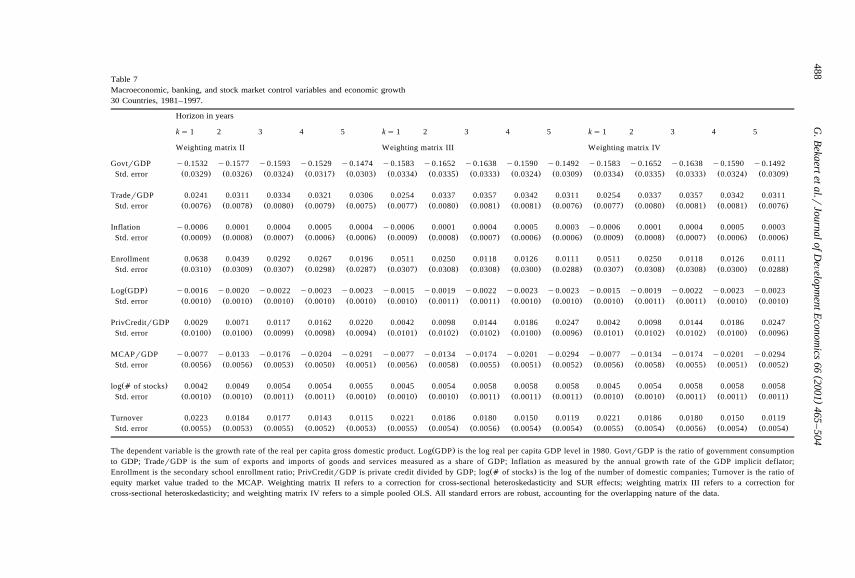
In Table 7, we present the estimated regression coefficients when we add thesethree measures of equity market development to the control variables presentedabove, including the measure of banking development. The estimated relationbetween the macro economic variables and economic growth is qualitatively andquantitatively affected by the inclusion of the three equity market variables. ThegovernmentrGDP and traderGDP variables have now generally a larger sign, andare economically and statistically significant. The inflation effect has lost robust-ness across specifications. The enrollment variable is still important, but its effectis weaker both in an economic and statistical sense. The relation between initialGDP and economic growth is now negative and significant across almost allspecifications. Additionally, the measure of banking development is now posi-tively and significantly related to growth at longer horizons, which is consistent
Ž .with the evidence presented in King and Levine 1993 and Levine and ZervosŽ .1998 . The coefficient on equity market size is generally negative and significantwhich is the opposite to what was expected. Additionally, the relation between thelogged number of companies and the rate of economic growth is positive andsignificant. In accordance with the evidence presented in Levine and ZervosŽ .1998 , the relationship between turnover and economic growth is positive andsignificant in nearly all cases.
4.3. The liberalization effect with control Õariables
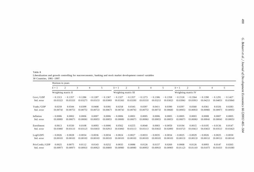
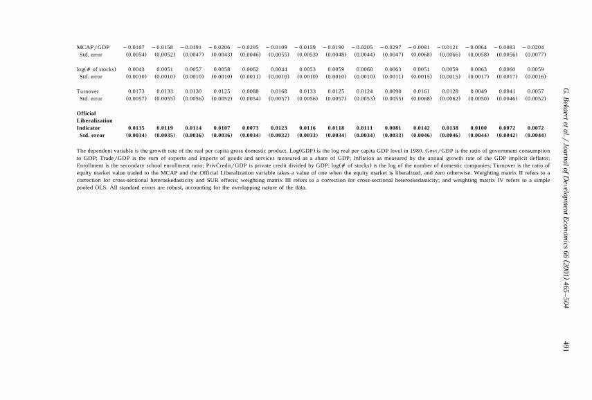
Having potentially controlled for unrelated phenomena by using the macroeco-nomic, banking sector, and equity market variables employed in the existinggrowth literature, we return to the relationship between economic growth andfinancial liberalization, where again the latter is measured using the officialliberalization indicator. Table 8 presents the regressions with the financial liberal-ization indicator and all the control variables. The results in Table 8 show that theestimated relation between the control variables and economic growth are gener-ally unaffected by the inclusion of the liberalization indicator. As before, therelation between economic growth and banking sector development is positive andsignificant only at longer horizons. The enrollment variable now proves fragile.However, it is striking that across all weighting matrix specifications, financial
()
G.B
ekaertetal.r
JournalofD
eÕelopm
entEconom
ics66
2001465
–504
488
Table 7Macroeconomic, banking, and stock market control variables and economic growth30 Countries, 1981–1997.
Horizon in years
ks 1 2 3 4 5 ks 1 2 3 4 5 ks 1 2 3 4 5
Weighting matrix II Weighting matrix III Weighting matrix IV
GovtrGDP y0.1532 y0.1577 y0.1593 y0.1529 y0.1474 y0.1583 y0.1652 y0.1638 y0.1590 y0.1492 y0.1583 y0.1652 y0.1638 y0.1590 y0.1492Ž . Ž . Ž . Ž . Ž . Ž . Ž . Ž . Ž . Ž . Ž . Ž . Ž . Ž . Ž .Std. error 0.0329 0.0326 0.0324 0.0317 0.0303 0.0334 0.0335 0.0333 0.0324 0.0309 0.0334 0.0335 0.0333 0.0324 0.0309
TraderGDP 0.0241 0.0311 0.0334 0.0321 0.0306 0.0254 0.0337 0.0357 0.0342 0.0311 0.0254 0.0337 0.0357 0.0342 0.0311Ž . Ž . Ž . Ž . Ž . Ž . Ž . Ž . Ž . Ž . Ž . Ž . Ž . Ž . Ž .Std. error 0.0076 0.0078 0.0080 0.0079 0.0075 0.0077 0.0080 0.0081 0.0081 0.0076 0.0077 0.0080 0.0081 0.0081 0.0076
Inflation y0.0006 0.0001 0.0004 0.0005 0.0004 y0.0006 0.0001 0.0004 0.0005 0.0003 y0.0006 0.0001 0.0004 0.0005 0.0003Ž . Ž . Ž . Ž . Ž . Ž . Ž . Ž . Ž . Ž . Ž . Ž . Ž . Ž . Ž .Std. error 0.0009 0.0008 0.0007 0.0006 0.0006 0.0009 0.0008 0.0007 0.0006 0.0006 0.0009 0.0008 0.0007 0.0006 0.0006
Enrollment 0.0638 0.0439 0.0292 0.0267 0.0196 0.0511 0.0250 0.0118 0.0126 0.0111 0.0511 0.0250 0.0118 0.0126 0.0111Ž . Ž . Ž . Ž . Ž . Ž . Ž . Ž . Ž . Ž . Ž . Ž . Ž . Ž . Ž .Std. error 0.0310 0.0309 0.0307 0.0298 0.0287 0.0307 0.0308 0.0308 0.0300 0.0288 0.0307 0.0308 0.0308 0.0300 0.0288
Ž .Log GDP y0.0016 y0.0020 y0.0022 y0.0023 y0.0023 y0.0015 y0.0019 y0.0022 y0.0023 y0.0023 y0.0015 y0.0019 y0.0022 y0.0023 y0.0023Ž . Ž . Ž . Ž . Ž . Ž . Ž . Ž . Ž . Ž . Ž . Ž . Ž . Ž . Ž .Std. error 0.0010 0.0010 0.0010 0.0010 0.0010 0.0010 0.0011 0.0011 0.0010 0.0010 0.0010 0.0011 0.0011 0.0010 0.0010
PrivCreditrGDP 0.0029 0.0071 0.0117 0.0162 0.0220 0.0042 0.0098 0.0144 0.0186 0.0247 0.0042 0.0098 0.0144 0.0186 0.0247Ž . Ž . Ž . Ž . Ž . Ž . Ž . Ž . Ž . Ž . Ž . Ž . Ž . Ž . Ž .Std. error 0.0100 0.0100 0.0099 0.0098 0.0094 0.0101 0.0102 0.0102 0.0100 0.0096 0.0101 0.0102 0.0102 0.0100 0.0096
MCAPrGDP y0.0077 y0.0133 y0.0176 y0.0204 y0.0291 y0.0077 y0.0134 y0.0174 y0.0201 y0.0294 y0.0077 y0.0134 y0.0174 y0.0201 y0.0294Ž . Ž . Ž . Ž . Ž . Ž . Ž . Ž . Ž . Ž . Ž . Ž . Ž . Ž . Ž .Std. error 0.0056 0.0056 0.0053 0.0050 0.0051 0.0056 0.0058 0.0055 0.0051 0.0052 0.0056 0.0058 0.0055 0.0051 0.0052
Ž .log a of stocks 0.0042 0.0049 0.0054 0.0054 0.0055 0.0045 0.0054 0.0058 0.0058 0.0058 0.0045 0.0054 0.0058 0.0058 0.0058Ž . Ž . Ž . Ž . Ž . Ž . Ž . Ž . Ž . Ž . Ž . Ž . Ž . Ž . Ž .Std. error 0.0010 0.0010 0.0011 0.0011 0.0010 0.0010 0.0010 0.0011 0.0011 0.0011 0.0010 0.0010 0.0011 0.0011 0.0011
Turnover 0.0223 0.0184 0.0177 0.0143 0.0115 0.0221 0.0186 0.0180 0.0150 0.0119 0.0221 0.0186 0.0180 0.0150 0.0119Ž . Ž . Ž . Ž . Ž . Ž . Ž . Ž . Ž . Ž . Ž . Ž . Ž . Ž . Ž .Std. error 0.0055 0.0053 0.0055 0.0052 0.0053 0.0055 0.0054 0.0056 0.0054 0.0054 0.0055 0.0054 0.0056 0.0054 0.0054
Ž .The dependent variable is the growth rate of the real per capita gross domestic product. Log GDP is the log real per capita GDP level in 1980. GovtrGDP is the ratio of government consumptionto GDP; TraderGDP is the sum of exports and imports of goods and services measured as a share of GDP; Inflation as measured by the annual growth rate of the GDP implicit deflator;
Ž .Enrollment is the secondary school enrollment ratio; PrivCreditrGDP is private credit divided by GDP; log a of stocks is the log of the number of domestic companies; Turnover is the ratio ofequity market value traded to the MCAP. Weighting matrix II refers to a correction for cross-sectional heteroskedasticity and SUR effects; weighting matrix III refers to a correction forcross-sectional heteroskedasticity; and weighting matrix IV refers to a simple pooled OLS. All standard errors are robust, accounting for the overlapping nature of the data.

( )G. Bekaert et al.rJournal of DeÕelopment Economics 66 2001 465–504 489
liberalization is associated with a higher level of real economic growth. Theevidence implies that real GDP per capita growth rates increase following finan-cial liberalization by anywhere from 0.7% to as large as 1.4% per annum. Despitethe large Monte Carlo critical values presented in the table in Appendix C, theseestimates retain statistical significance at the 95% confidence level in many of thespecifications considered.
Overall, the evidence presented in Table 8 suggests that on average realeconomic growth rates increase roughly 1.1% per annum following financialliberalization. This finding is consistent with that presented in Table 4, when nocontrol variables are employed, suggesting the relation between financial liberal-ization and economic growth is robust across weighting matrix specifications and
Ž .conditioning variables. Levine and Renelt 1992 demonstrate that the estimatedcoefficients in cross-country regressions require extreme caution in interpretation,as they are sensitive to the set of control variables employed. Consequently, theevidence presented in Table 8 strengthens the argument that financial liberalizationexplains an important part of the cross-sectional and time-series characteristics ofreal economic growth.
Surprisingly, the patterns in the coefficients across the different horizonssuggest that the strongest growth impacts are experienced shortly after liberaliza-tion. For example, for weighting matrix III in Table 8, the coefficients for the 1- to5-year horizons are: 0.0123, 0.0116, 0.0118, 0.0111, and 0.0081. This suggeststhat the total impact on economic growth over the 5-year period is 4.1%. Over half
Ž .of the additional growth 2.3% occurs in the first 2 years and 87% of the 5-yeargrowth impact occurs in the first 3 years.
4.4. Robustness
We explore five experiments that are designed to test the robustness of theliberalization indicator effect on future economic growth.
First, we consider an alternative specification that allows for regional differ-ences in the measured effect of financial liberalization on economic growth. Inparticular, the high level of economic growth observed in Latin American coun-tries after the debt crisis may significantly affect the relationship between liberal-ization and growth discussed above. Although this higher growth after the AlostdecadeB may be due in part to financial liberalization, this is open to debate.Therefore, we explore whether Latin American countries drive our results byestimating the following regional regression equation:
Y sbXx qd lib indicator =LatinŽ .i , tqk ,k i , t 1 i , t i
qd lib indicator = 1yLatin qe , 32Ž . Ž .Ž .2 i , t i i , tqk ,k
where Latin takes the value of 1 if country i is a Latin American country, and 0i
otherwise. This specification allow the relationship between financial liberalization
()
G.B
ekaertetal.r
JournalofD
eÕelopm
entEconom
ics66
2001465
–504
490
Table 8Liberalization and growth controlling for macroeconomic, banking and stock market development control variables30 Countries, 1981–1997.
Horizon in years
ks 1 2 3 4 5 ks 1 2 3 4 5 ks 1 2 3 4 5
Weighting matrix II Weighting matrix III Weighting matrix IV
GovtrGDP y0.1313 y0.1357 y0.1286 y0.1287 y0.1367 y0.1327 y0.1357 y0.1273 y0.1306 y0.1358 y0.1518 y0.1564 y0.1390 y0.1291 y0.1427Ž . Ž . Ž . Ž . Ž . Ž . Ž . Ž . Ž . Ž . Ž . Ž . Ž . Ž . Ž .Std. error 0.0332 0.0333 0.0327 0.0315 0.0300 0.0336 0.0339 0.0333 0.0321 0.0302 0.0396 0.0391 0.0421 0.0405 0.0384
TraderGDP 0.0259 0.0344 0.0399 0.0408 0.0395 0.0258 0.0345 0.0397 0.0411 0.0390 0.0297 0.0360 0.0361 0.0326 0.0283Ž . Ž . Ž . Ž . Ž . Ž . Ž . Ž . Ž . Ž . Ž . Ž . Ž . Ž . Ž .Std. error 0.0074 0.0075 0.0075 0.0072 0.0067 0.0074 0.0076 0.0075 0.0073 0.0068 0.0095 0.0093 0.0098 0.0097 0.0095
Inflation y0.0006 0.0002 0.0006 0.0007 0.0006 y0.0006 0.0001 0.0005 0.0006 0.0005 y0.0005 0.0003 0.0008 0.0007 0.0005Ž . Ž . Ž . Ž . Ž . Ž . Ž . Ž . Ž . Ž . Ž . Ž . Ž . Ž . Ž .Std. error 0.0008 0.0007 0.0006 0.0005 0.0005 0.0008 0.0007 0.0006 0.0005 0.0005 0.0007 0.0006 0.0004 0.0004 0.0005
Enrollment 0.0613 0.0330 0.0108 0.0093 y0.0006 0.0562 0.0255 0.0040 0.0003 y0.0059 0.0194 0.0015 y0.0195 y0.0136 0.0147Ž . Ž . Ž . Ž . Ž . Ž . Ž . Ž . Ž . Ž . Ž . Ž . Ž . Ž . Ž .Std. error 0.0308 0.0313 0.0312 0.0303 0.0291 0.0306 0.0311 0.0311 0.0302 0.0289 0.0372 0.0361 0.0365 0.0351 0.0342
Ž .Log GDP y0.0026 y0.0028 y0.0034 y0.0036 y0.0034 y0.0024 y0.0027 y0.0033 y0.0035 y0.0034 y0.0025 y0.0029 y0.0026 y0.0025 y0.0030Ž . Ž . Ž . Ž . Ž . Ž . Ž . Ž . Ž . Ž . Ž . Ž . Ž . Ž . Ž .Std. error 0.0010 0.0010 0.0010 0.0010 0.0010 0.0010 0.0010 0.0010 0.0010 0.0010 0.0013 0.0013 0.0015 0.0015 0.0014
PrivCreditrGDP 0.0025 0.0075 0.0112 0.0143 0.0252 0.0035 0.0086 0.0126 0.0157 0.0269 0.0068 0.0126 0.0093 0.0147 0.0265Ž . Ž . Ž . Ž . Ž . Ž . Ž . Ž . Ž . Ž . Ž . Ž . Ž . Ž . Ž .Std. error 0.0097 0.0097 0.0093 0.0092 0.0089 0.0098 0.0098 0.0095 0.0093 0.0090 0.0112 0.0110 0.0107 0.0103 0.0108
()
G.B
ekaertetal.r
JournalofD
eÕelopm
entEconom
ics66
2001465
–504
491
MCAPrGDP y0.0107 y0.0158 y0.0191 y0.0206 y0.0295 y0.0109 y0.0159 y0.0190 y0.0205 y0.0297 y0.0081 y0.0121 y0.0064 y0.0083 y0.0204Ž . Ž . Ž . Ž . Ž . Ž . Ž . Ž . Ž . Ž . Ž . Ž . Ž . Ž . Ž .Std. error 0.0054 0.0052 0.0047 0.0043 0.0046 0.0055 0.0053 0.0048 0.0044 0.0047 0.0068 0.0066 0.0058 0.0056 0.0077
Ž .log a of stocks 0.0043 0.0051 0.0057 0.0058 0.0062 0.0044 0.0053 0.0059 0.0060 0.0063 0.0051 0.0059 0.0063 0.0060 0.0059Ž . Ž . Ž . Ž . Ž . Ž . Ž . Ž . Ž . Ž . Ž . Ž . Ž . Ž . Ž .Std. error 0.0010 0.0010 0.0010 0.0010 0.0011 0.0010 0.0010 0.0010 0.0010 0.0011 0.0015 0.0015 0.0017 0.0017 0.0016
Turnover 0.0173 0.0133 0.0130 0.0125 0.0088 0.0168 0.0133 0.0125 0.0124 0.0090 0.0161 0.0128 0.0049 0.0041 0.0057Ž . Ž . Ž . Ž . Ž . Ž . Ž . Ž . Ž . Ž . Ž . Ž . Ž . Ž . Ž .Std. error 0.0057 0.0055 0.0056 0.0052 0.0054 0.0057 0.0056 0.0057 0.0053 0.0055 0.0068 0.0062 0.0050 0.0046 0.0052
OfficialLiberalizationIndicator 0.0135 0.0119 0.0114 0.0107 0.0073 0.0123 0.0116 0.0118 0.0111 0.0081 0.0142 0.0138 0.0100 0.0072 0.0072
Ž . Ž . Ž . Ž . Ž . Ž . Ž . Ž . Ž . Ž . Ž . Ž . Ž . Ž . Ž .Std. error 0.0034 0.0035 0.0036 0.0036 0.0034 0.0032 0.0033 0.0034 0.0034 0.0033 0.0046 0.0046 0.0044 0.0042 0.0044
Ž .The dependent variable is the growth rate of the real per capita gross domestic product. Log GDP is the log real per capita GDP level in 1980. GovtrGDP is the ratio of government consumptionto GDP; TraderGDP is the sum of exports and imports of goods and services measured as a share of GDP; Inflation as measured by the annual growth rate of the GDP implicit deflator;
Ž .Enrollment is the secondary school enrollment ratio; PrivCreditrGDP is private credit divided by GDP; log a of stocks is the log of the number of domestic companies; Turnover is the ratio ofequity market value traded to the MCAP and the Official Liberalization variable takes a value of one when the equity market is liberalized, and zero otherwise. Weighting matrix II refers to acorrection for cross-sectional heteroskedasticity and SUR effects; weighting matrix III refers to a correction for cross-sectional heteroskedasticity; and weighting matrix IV refers to a simplepooled OLS. All standard errors are robust, accounting for the overlapping nature of the data.

( )G. Bekaert et al.rJournal of DeÕelopment Economics 66 2001 465–504492
and economic growth to differ across Latin American and non-Latin Americancountries.
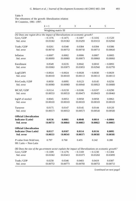
Given the evidence presented in the first panel of Table 9 for these estimatedregressions, the regional effect is negligible. If anything, the growth effect appearsconsiderably weaker in Latin American countries relative to other countries. This
Žsuggests that the observed liberalization effect discussed above and presented in.Table 8 is not being driven by regional economic success in Latin America during
our sample period.Second, we examine the role of the government sector. Is it the case that the
impact of liberalization on economic growth is determined by the size of thegovernment sector? We create a variable, BigGov, that takes on the value of one ifthe country-specific median government spending to GDP ratio is greater than allcountries’ median government spending to GDP ratio. We run a regression similarto the regional regression above which splits the liberalization indicator into twopieces.
The results in the Panel B of Table 9 show that the financial liberalizationvariable retains it significance and magnitude for both sets of countries. Theliberalization effect is 25 basis points larger for countries with smaller than mediangovernment sectors. However, the difference is not statistically significant. Inunreported results, we also estimated a regression adding an interaction termŽ .liberalization times the government sector to GDP ratio . The coefficient on theinteraction term was insignificant, further strengthening the case that there is norelation between the size of the government sector and the impact of liberalizationon real economic growth.
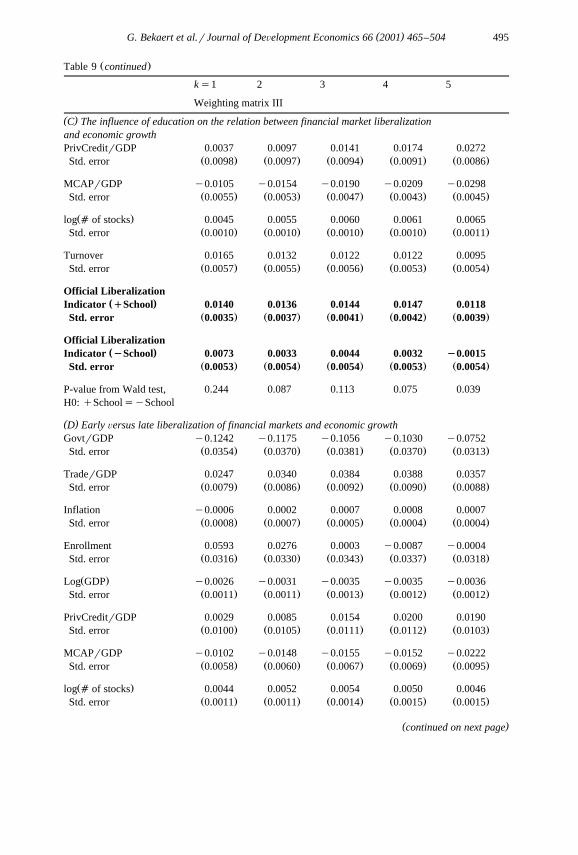
The third experiment examines the role of education. It is possible thatcountries with higher levels of education could stand to benefit more fromfinancial market liberalizations than countries with low levels of education.Similar to the method for the size of the government sector, we created a variable,School, which takes on a value of unity if the country-specific median secondaryschool enrollment is greater than the whole sample median secondary schoolenrollment.
The results are presented in Panel C of Table 9. It is clear from these resultsthat countries with high levels of education stand to benefit more from financialmarket liberalizations. For example, in the 3-year horizon for all three weightingmatrices, the coefficient on the liberalization indicator is three times larger forcountries with above median education levels. The results suggest that policymakers should not expect a large growth impact from liberalization if thecountry’s education level is lower than the median in these 30 emerging markets.The Wald tests show that the difference between the two liberalization effects isstatistically significant in the longer horizon regressions.
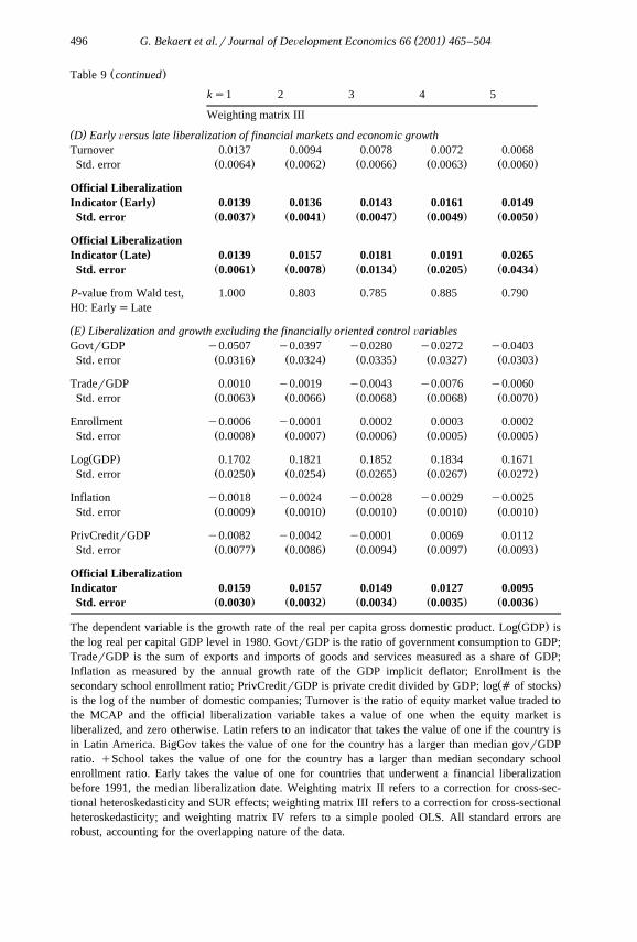
The fourth experiment focuses on early versus late liberalizers. Is it the casethat most of the growth benefits occurred for the early liberalizers? This ispossible if only limited capital from the developed world is available and that it
( )G. Bekaert et al.rJournal of DeÕelopment Economics 66 2001 465–504 493
Table 9The robustness of the growth–liberalization relation30 Countries, 1981–1997.
ks1 2 3 4 5
Weighting matrix III
( )A Does one region driÕe the impact of liberalizations on economic growth?GovtrGDP y0.1376 y0.1475 y0.1407 y0.1416 y0.1520
Ž . Ž . Ž . Ž . Ž .Std. error 0.0336 0.0336 0.0329 0.0315 0.0294
TraderGDP 0.0261 0.0340 0.0384 0.0394 0.0386Ž . Ž . Ž . Ž . Ž .Std. error 0.0074 0.0075 0.0074 0.0071 0.0064
Inflation y0.0007 0.0002 0.0006 0.0007 0.0005Ž . Ž . Ž . Ž . Ž .Std. error 0.0009 0.0008 0.0007 0.0006 0.0006
Enrollment 0.0549 0.0235 0.0042 0.0010 y0.0093Ž . Ž . Ž . Ž . Ž .Std. error 0.0306 0.0307 0.0305 0.0294 0.0279
Ž .Log GDP y0.0024 y0.0024 y0.0028 y0.0030 y0.0029Ž . Ž . Ž . Ž . Ž .Std. error 0.0010 0.0010 0.0011 0.0011 0.0011
PrivCreditrGDP 0.0050 0.0095 0.0123 0.0145 0.0256Ž . Ž . Ž . Ž . Ž .Std. error 0.0098 0.0098 0.0094 0.0092 0.0088
MCAPrGDP y0.0114 y0.0159 y0.0186 y0.0197 y0.0290Ž . Ž . Ž . Ž . Ž .Std. error 0.0055 0.0053 0.0047 0.0043 0.0046
Ž .log a of stocks 0.0045 0.0053 0.0058 0.0058 0.0063Ž . Ž . Ž . Ž . Ž .Std. error 0.0010 0.0010 0.0010 0.0010 0.0010
Turnover 0.0175 0.0147 0.0145 0.0144 0.0120Ž . Ž . Ž . Ž . Ž .Std. error 0.0057 0.0055 0.0057 0.0054 0.0058
Official Liberalization( )Indicator Latin 0.0136 0.0081 0.0048 0.0014 I0.0004
Ž . Ž . Ž . Ž . Ž .Std. error 0.0073 0.0084 0.0085 0.0082 0.0085
Official Liberalization( )Indicator Non-Latin 0.0117 0.0107 0.0114 0.0116 0.0095
Ž . Ž . Ž . Ž . Ž .Std. error 0.0033 0.0034 0.0037 0.0038 0.0038
P-value from Wald test, 0.797 0.760 0.455 0.242 0.280H0: LatinsNon-Latin
( )B Does the size of the goÕernment sector explain the impact of liberalizations on economic growth?GovtrGDP y0.1309 y0.1276 y0.1169 y0.1230 y0.1304
Ž . Ž . Ž . Ž . Ž .Std. error 0.0336 0.0341 0.0337 0.0326 0.0309
TraderGDP 0.0258 0.0346 0.0403 0.0419 0.0387Ž . Ž . Ž . Ž . Ž .Std. error 0.0075 0.0077 0.0078 0.0075 0.0071
( )continued on next page

( )G. Bekaert et al.rJournal of DeÕelopment Economics 66 2001 465–504494
Ž .Table 9 continued
ks1 2 3 4 5
Weighting matrix III
( )B Does the size of the goÕernment sector explain the impact of liberalizations on economic growth?Inflation y0.0006 0.0002 0.0006 0.0006 0.0005
Ž . Ž . Ž . Ž . Ž .Std. error 0.0008 0.0007 0.0006 0.0005 0.0004
Enrollment 0.0566 0.0240 y0.0026 y0.0071 y0.0106Ž . Ž . Ž . Ž . Ž .Std. error 0.0309 0.0319 0.0322 0.0313 0.0300
Ž .Log GDP y0.0025 y0.0029 y0.0035 y0.0035 y0.0032Ž . Ž . Ž . Ž . Ž .Std. error 0.0010 0.0010 0.0010 0.0010 0.0010
PrivCreditrGDP 0.0034 0.0083 0.0133 0.0169 0.0269Ž . Ž . Ž . Ž . Ž .Std. error 0.0098 0.0100 0.0098 0.0096 0.0092
MCAPrGDP y0.0109 y0.0158 y0.0194 y0.0215 y0.0303Ž . Ž . Ž . Ž . Ž .Std. error 0.0056 0.0054 0.0049 0.0045 0.0047
Ž .log a of stocks 0.0044 0.0053 0.0060 0.0061 0.0061Ž . Ž . Ž . Ž . Ž .Std. error 0.0010 0.0010 0.0010 0.0010 0.0010
Turnover 0.0166 0.0121 0.0108 0.0109 0.0080Ž . Ž . Ž . Ž . Ž .Std. error 0.0057 0.0056 0.0057 0.0053 0.0054
Official Liberalization( )Indicator Big Gov. 0.0128 0.0122 0.0119 0.0117 0.0080
Ž . Ž . Ž . Ž . Ž .Std. error 0.0045 0.0047 0.0047 0.0046 0.0041
Official Liberalization( )Indicator Small Gov. 0.0122 0.0127 0.0144 0.0134 0.0093
Ž . Ž . Ž . Ž . Ž .Std. error 0.0039 0.0042 0.0045 0.0047 0.0049
P-value from Wald test, 0.920 0.926 0.681 0.792 0.829H0: Big Gov.sSmall Gov.
( )C The influence of education on the relation between financial market liberalizationand economic growthGovtrGDP y0.1283 y0.1322 y0.1218 y0.1256 y0.1338
Ž . Ž . Ž . Ž . Ž .Std. error 0.0337 0.0336 0.0328 0.0313 0.0294
TraderGDP 0.0252 0.0341 0.0393 0.0406 0.0389Ž . Ž . Ž . Ž . Ž .Std. error 0.0075 0.0075 0.0075 0.0071 0.0065
Inflation y0.0005 0.0002 0.0005 0.0006 0.0004Ž . Ž . Ž . Ž . Ž .Std. error 0.0008 0.0007 0.0006 0.0005 0.0005
Enrollment 0.0502 0.0138 y0.0051 y0.0093 y0.0166Ž . Ž . Ž . Ž . Ž .Std. error 0.0307 0.0309 0.0308 0.0296 0.0281
Ž .Log GDP y0.0023 y0.0026 y0.0033 y0.0034 y0.0033Ž . Ž . Ž . Ž . Ž .Std. error 0.0010 0.0010 0.0010 0.0010 0.0010
( )G. Bekaert et al.rJournal of DeÕelopment Economics 66 2001 465–504 495
Ž .Table 9 continued
ks1 2 3 4 5
Weighting matrix III
( )C The influence of education on the relation between financial market liberalizationand economic growthPrivCreditrGDP 0.0037 0.0097 0.0141 0.0174 0.0272
Ž . Ž . Ž . Ž . Ž .Std. error 0.0098 0.0097 0.0094 0.0091 0.0086
MCAPrGDP y0.0105 y0.0154 y0.0190 y0.0209 y0.0298Ž . Ž . Ž . Ž . Ž .Std. error 0.0055 0.0053 0.0047 0.0043 0.0045
Ž .log a of stocks 0.0045 0.0055 0.0060 0.0061 0.0065Ž . Ž . Ž . Ž . Ž .Std. error 0.0010 0.0010 0.0010 0.0010 0.0011
Turnover 0.0165 0.0132 0.0122 0.0122 0.0095Ž . Ž . Ž . Ž . Ž .Std. error 0.0057 0.0055 0.0056 0.0053 0.0054
Official Liberalization( )Indicator HSchool 0.0140 0.0136 0.0144 0.0147 0.0118
Ž . Ž . Ž . Ž . Ž .Std. error 0.0035 0.0037 0.0041 0.0042 0.0039
Official Liberalization( )Indicator ISchool 0.0073 0.0033 0.0044 0.0032 I0.0015
Ž . Ž . Ž . Ž . Ž .Std. error 0.0053 0.0054 0.0054 0.0053 0.0054
P-value from Wald test, 0.244 0.087 0.113 0.075 0.039H0: qSchoolsySchool
( )D Early Õersus late liberalization of financial markets and economic growthGovtrGDP y0.1242 y0.1175 y0.1056 y0.1030 y0.0752
Ž . Ž . Ž . Ž . Ž .Std. error 0.0354 0.0370 0.0381 0.0370 0.0313
TraderGDP 0.0247 0.0340 0.0384 0.0388 0.0357Ž . Ž . Ž . Ž . Ž .Std. error 0.0079 0.0086 0.0092 0.0090 0.0088
Inflation y0.0006 0.0002 0.0007 0.0008 0.0007Ž . Ž . Ž . Ž . Ž .Std. error 0.0008 0.0007 0.0005 0.0004 0.0004
Enrollment 0.0593 0.0276 0.0003 y0.0087 y0.0004Ž . Ž . Ž . Ž . Ž .Std. error 0.0316 0.0330 0.0343 0.0337 0.0318
Ž .Log GDP y0.0026 y0.0031 y0.0035 y0.0035 y0.0036Ž . Ž . Ž . Ž . Ž .Std. error 0.0011 0.0011 0.0013 0.0012 0.0012
PrivCreditrGDP 0.0029 0.0085 0.0154 0.0200 0.0190Ž . Ž . Ž . Ž . Ž .Std. error 0.0100 0.0105 0.0111 0.0112 0.0103
MCAPrGDP y0.0102 y0.0148 y0.0155 y0.0152 y0.0222Ž . Ž . Ž . Ž . Ž .Std. error 0.0058 0.0060 0.0067 0.0069 0.0095
Ž .log a of stocks 0.0044 0.0052 0.0054 0.0050 0.0046Ž . Ž . Ž . Ž . Ž .Std. error 0.0011 0.0011 0.0014 0.0015 0.0015
( )continued on next page
( )G. Bekaert et al.rJournal of DeÕelopment Economics 66 2001 465–504496
Ž .Table 9 continued
ks1 2 3 4 5
Weighting matrix III
( )D Early Õersus late liberalization of financial markets and economic growthTurnover 0.0137 0.0094 0.0078 0.0072 0.0068
Ž . Ž . Ž . Ž . Ž .Std. error 0.0064 0.0062 0.0066 0.0063 0.0060
Official Liberalization( )Indicator Early 0.0139 0.0136 0.0143 0.0161 0.0149
Ž . Ž . Ž . Ž . Ž .Std. error 0.0037 0.0041 0.0047 0.0049 0.0050
Official Liberalization( )Indicator Late 0.0139 0.0157 0.0181 0.0191 0.0265
Ž . Ž . Ž . Ž . Ž .Std. error 0.0061 0.0078 0.0134 0.0205 0.0434
P-value from Wald test, 1.000 0.803 0.785 0.885 0.790H0: EarlysLate
( )E Liberalization and growth excluding the financially oriented control ÕariablesGovtrGDP y0.0507 y0.0397 y0.0280 y0.0272 y0.0403
Ž . Ž . Ž . Ž . Ž .Std. error 0.0316 0.0324 0.0335 0.0327 0.0303
TraderGDP 0.0010 y0.0019 y0.0043 y0.0076 y0.0060Ž . Ž . Ž . Ž . Ž .Std. error 0.0063 0.0066 0.0068 0.0068 0.0070
Enrollment y0.0006 y0.0001 0.0002 0.0003 0.0002Ž . Ž . Ž . Ž . Ž .Std. error 0.0008 0.0007 0.0006 0.0005 0.0005
Ž .Log GDP 0.1702 0.1821 0.1852 0.1834 0.1671Ž . Ž . Ž . Ž . Ž .Std. error 0.0250 0.0254 0.0265 0.0267 0.0272
Inflation y0.0018 y0.0024 y0.0028 y0.0029 y0.0025Ž . Ž . Ž . Ž . Ž .Std. error 0.0009 0.0010 0.0010 0.0010 0.0010
PrivCreditrGDP y0.0082 y0.0042 y0.0001 0.0069 0.0112Ž . Ž . Ž . Ž . Ž .Std. error 0.0077 0.0086 0.0094 0.0097 0.0093
Official LiberalizationIndicator 0.0159 0.0157 0.0149 0.0127 0.0095
Ž . Ž . Ž . Ž . Ž .Std. error 0.0030 0.0032 0.0034 0.0035 0.0036
Ž .The dependent variable is the growth rate of the real per capita gross domestic product. Log GDP isthe log real per capital GDP level in 1980. GovtrGDP is the ratio of government consumption to GDP;TraderGDP is the sum of exports and imports of goods and services measured as a share of GDP;Inflation as measured by the annual growth rate of the GDP implicit deflator; Enrollment is the
Ž .secondary school enrollment ratio; PrivCreditrGDP is private credit divided by GDP; log a of stocksis the log of the number of domestic companies; Turnover is the ratio of equity market value traded tothe MCAP and the official liberalization variable takes a value of one when the equity market isliberalized, and zero otherwise. Latin refers to an indicator that takes the value of one if the country isin Latin America. BigGov takes the value of one for the country has a larger than median govrGDPratio. qSchool takes the value of one for the country has a larger than median secondary schoolenrollment ratio. Early takes the value of one for countries that underwent a financial liberalizationbefore 1991, the median liberalization date. Weighting matrix II refers to a correction for cross-sec-tional heteroskedasticity and SUR effects; weighting matrix III refers to a correction for cross-sectionalheteroskedasticity; and weighting matrix IV refers to a simple pooled OLS. All standard errors arerobust, accounting for the overlapping nature of the data.
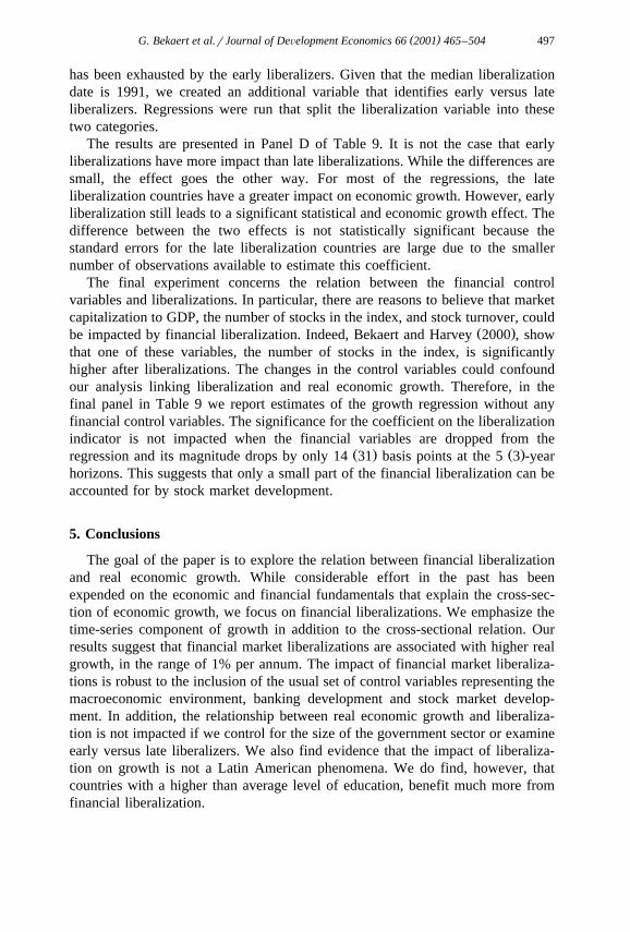
( )G. Bekaert et al.rJournal of DeÕelopment Economics 66 2001 465–504 497
has been exhausted by the early liberalizers. Given that the median liberalizationdate is 1991, we created an additional variable that identifies early versus lateliberalizers. Regressions were run that split the liberalization variable into thesetwo categories.
The results are presented in Panel D of Table 9. It is not the case that earlyliberalizations have more impact than late liberalizations. While the differences aresmall, the effect goes the other way. For most of the regressions, the lateliberalization countries have a greater impact on economic growth. However, earlyliberalization still leads to a significant statistical and economic growth effect. Thedifference between the two effects is not statistically significant because thestandard errors for the late liberalization countries are large due to the smallernumber of observations available to estimate this coefficient.
The final experiment concerns the relation between the financial controlvariables and liberalizations. In particular, there are reasons to believe that marketcapitalization to GDP, the number of stocks in the index, and stock turnover, could
Ž .be impacted by financial liberalization. Indeed, Bekaert and Harvey 2000 , showthat one of these variables, the number of stocks in the index, is significantlyhigher after liberalizations. The changes in the control variables could confoundour analysis linking liberalization and real economic growth. Therefore, in thefinal panel in Table 9 we report estimates of the growth regression without anyfinancial control variables. The significance for the coefficient on the liberalizationindicator is not impacted when the financial variables are dropped from the
Ž . Ž .regression and its magnitude drops by only 14 31 basis points at the 5 3 -yearhorizons. This suggests that only a small part of the financial liberalization can beaccounted for by stock market development.
5. Conclusions
The goal of the paper is to explore the relation between financial liberalizationand real economic growth. While considerable effort in the past has beenexpended on the economic and financial fundamentals that explain the cross-sec-tion of economic growth, we focus on financial liberalizations. We emphasize thetime-series component of growth in addition to the cross-sectional relation. Ourresults suggest that financial market liberalizations are associated with higher realgrowth, in the range of 1% per annum. The impact of financial market liberaliza-tions is robust to the inclusion of the usual set of control variables representing themacroeconomic environment, banking development and stock market develop-ment. In addition, the relationship between real economic growth and liberaliza-tion is not impacted if we control for the size of the government sector or examineearly versus late liberalizers. We also find evidence that the impact of liberaliza-tion on growth is not a Latin American phenomena. We do find, however, thatcountries with a higher than average level of education, benefit much more fromfinancial liberalization.
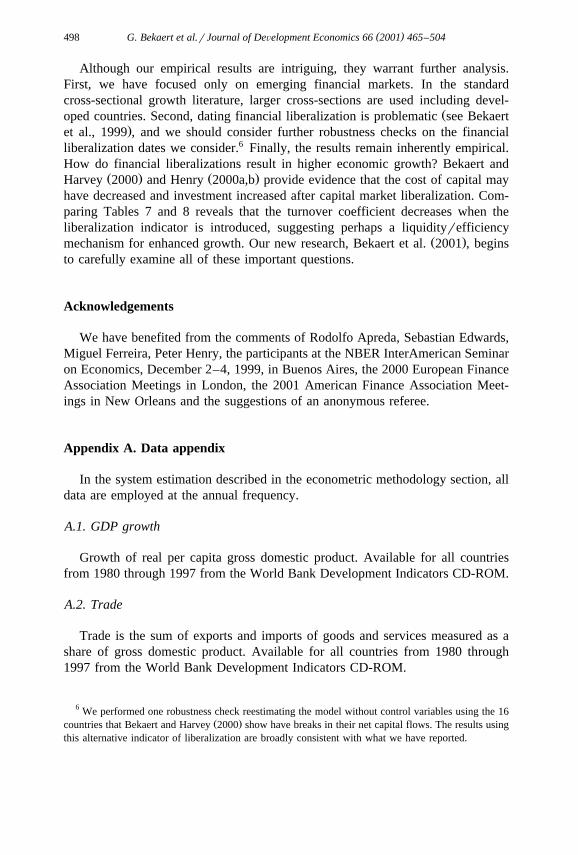
( )G. Bekaert et al.rJournal of DeÕelopment Economics 66 2001 465–504498
Although our empirical results are intriguing, they warrant further analysis.First, we have focused only on emerging financial markets. In the standardcross-sectional growth literature, larger cross-sections are used including devel-
Žoped countries. Second, dating financial liberalization is problematic see Bekaert.et al., 1999 , and we should consider further robustness checks on the financial
liberalization dates we consider.6 Finally, the results remain inherently empirical.How do financial liberalizations result in higher economic growth? Bekaert and
Ž . Ž .Harvey 2000 and Henry 2000a,b provide evidence that the cost of capital mayhave decreased and investment increased after capital market liberalization. Com-paring Tables 7 and 8 reveals that the turnover coefficient decreases when theliberalization indicator is introduced, suggesting perhaps a liquidityrefficiency
Ž .mechanism for enhanced growth. Our new research, Bekaert et al. 2001 , beginsto carefully examine all of these important questions.
Acknowledgements
We have benefited from the comments of Rodolfo Apreda, Sebastian Edwards,Miguel Ferreira, Peter Henry, the participants at the NBER InterAmerican Seminaron Economics, December 2–4, 1999, in Buenos Aires, the 2000 European FinanceAssociation Meetings in London, the 2001 American Finance Association Meet-ings in New Orleans and the suggestions of an anonymous referee.
Appendix A. Data appendix
In the system estimation described in the econometric methodology section, alldata are employed at the annual frequency.
A.1. GDP growth
Growth of real per capita gross domestic product. Available for all countriesfrom 1980 through 1997 from the World Bank Development Indicators CD-ROM.
A.2. Trade
Trade is the sum of exports and imports of goods and services measured as ashare of gross domestic product. Available for all countries from 1980 through1997 from the World Bank Development Indicators CD-ROM.
6 We performed one robustness check reestimating the model without control variables using the 16Ž .countries that Bekaert and Harvey 2000 show have breaks in their net capital flows. The results using
this alternative indicator of liberalization are broadly consistent with what we have reported.

( )G. Bekaert et al.rJournal of DeÕelopment Economics 66 2001 465–504 499
A.3. GoÕernment consumption
Government consumption divided by gross domestic product. General govern-ment consumption includes all current expenditures for purchases of goods andservices by all levels of government, excluding most government enterprises. Italso includes capital expenditure on national defense and security. Available for allcountries from 1980 through 1997 from the World Bank Development IndicatorsCD-ROM.
A.4. Inflation
Inflation as measured by the annual growth rate of the gross domestic productimplicit deflator. Available for all countries from 1980 through 1997 from theWorld Bank Development Indicators CD-ROM.
A.5. Secondary School Enrollment
Secondary school enrollment ratio is the ratio of total enrollment, regardless ofage, to the population of the age group that officially corresponds to the level ofeducation shown. Available for all countries from 1980 through 1997 from theWorld Bank Development Indicators CD-ROM.
A.6. PriÕate credit
Private credit divided by gross domestic product. Credit to private sector refersto financial resources provided to the private sector, such as through loans,purchases of non-equity securities, and trade credits and other accounts receivablethat establish a claim for repayment. Available for all countries from 1980 through1997 from the World Bank Development Indicators CD-ROM.
A.7. Market capitalization
Equity market capitalization divided by gross domestic product. Equity marketcapitalization is from the International Finance Corporation’s Emerging StockMarkets Factbook. The gross domestic product data are from the World BankDevelopment Indicators CD-ROM. Data are available from 1980 through 1997.
A.8. Number of companies
The log of the number of domestic companies covered taken from the Interna-Ž .tional Finance Corporation’s IFC, 1997 Emerging Stock Markets Factbook. The
data are available from 1980 through 1997.
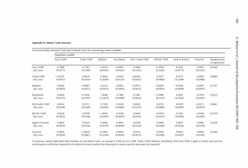
()
G.B
ekaertetal.r
JournalofD
eÕelopm
entEconom
ics66
2001465
–504
500
Appendix B. Monte Carlo structure
Cross-sectionally restricted VAR used in Monte Carlo for constructing control variables
Dependent variable
Ž .GovtrGDP TraderGDP Inflation Enrollment Priv CreditrGDP MCAPrGDP ln a of stocks Turnover Standard errorof regressions
GovtrGDP 0.7988 y0.1783 y2.3019 y0.0852 0.1893 y0.1034 0.2191 0.3057 0.0140Ž . Ž . Ž . Ž . Ž . Ž . Ž . Ž .Std. error 0.0277 0.1190 4.0191 0.0423 0.1313 0.3332 0.4771 0.3251
TraderGDP y0.0167 0.8419 0.2663 0.0202 y0.0103 0.3277 0.0275 0.0625 0.0600Ž . Ž . Ž . Ž . Ž . Ž . Ž . Ž .Std. error 0.0072 0.0310 1.0478 0.0110 0.0342 0.0869 0.1244 0.0848
Inflation 0.0002 y0.0007 0.4115 0.0001 y0.0073 y0.0005 y0.0038 y0.0007 0.1727Ž . Ž . Ž . Ž . Ž . Ž . Ž . Ž .Std. error 0.0003 0.0012 0.0413 0.0004 0.0013 0.0034 0.0049 0.0033
Enrollment 0.0450 y0.1816 1.4580 0.7489 0.1481 y0.2998 0.2667 0.1919 0.0213Ž . Ž . Ž . Ž . Ž . Ž . Ž . Ž .Std. error 0.0176 0.0755 2.5479 0.0268 0.0832 0.2112 0.3024 0.2061
PrivCreditrGDP 0.0014 0.0711 3.7194 y0.0149 0.8204 0.0791 0.0378 y0.0271 0.0661Ž . Ž . Ž . Ž . Ž . Ž . Ž . Ž .Std. error 0.0058 0.0249 0.8395 0.0088 0.0274 0.0696 0.0997 0.0679
MCAPrGDP 0.0018 0.0358 y1.0816 0.0158 0.0640 0.6374 0.1365 0.0954 0.1679Ž . Ž . Ž . Ž . Ž . Ž . Ž . Ž .Std. error 0.0035 0.0148 0.5005 0.0053 0.0163 0.0415 0.0594 0.0405
Ž .log a of stocks 0.0043 0.0310 0.2683 0.0091 0.0158 0.0403 0.4857 0.0966 0.1638Ž . Ž . Ž . Ž . Ž . Ž . Ž . Ž .Std. error 0.0032 0.0136 0.4579 0.0048 0.0150 0.0380 0.0543 0.0370
Turnover y0.0029 y0.0018 y0.1983 y0.0039 0.0124 0.0109 0.0633 0.8694 0.2404Ž . Ž . Ž . Ž . Ž . Ž . Ž . Ž .Std. error 0.0016 0.0067 0.2246 0.0024 0.0073 0.0186 0.0267 0.0182
Ž . Ž .To generate control right-hand side variables for our Monte Carlo, we estimate a VAR on GovrGDP, TraderGDP, Inflation, Enrollment, PrivCredrGDP, Log a of stocks , and turnover,Ž . Ž .restricting the coefficients reported to be identical across countries but allowing for country specific intercepts not reported .
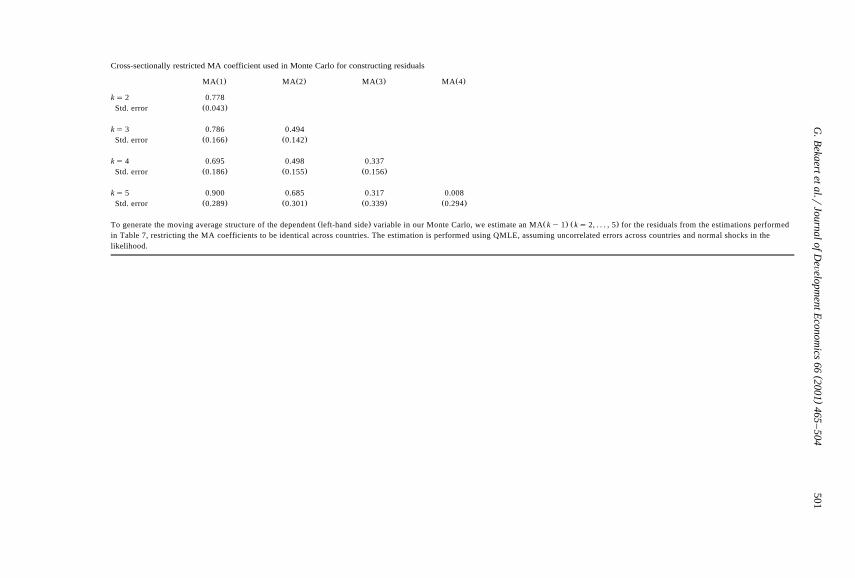
()
G.B
ekaertetal.r
JournalofD
eÕelopm
entEconom
ics66
2001465
–504
501
Cross-sectionally restricted MA coefficient used in Monte Carlo for constructing residuals
Ž . Ž . Ž . Ž .MA 1 MA 2 MA 3 MA 4
ks 2 0.778Ž .Std. error 0.043
ks 3 0.786 0.494Ž . Ž .Std. error 0.166 0.142
ks 4 0.695 0.498 0.337Ž . Ž . Ž .Std. error 0.186 0.155 0.156
ks 5 0.900 0.685 0.317 0.008Ž . Ž . Ž . Ž .Std. error 0.289 0.301 0.339 0.294
Ž . Ž . Ž .To generate the moving average structure of the dependent left-hand side variable in our Monte Carlo, we estimate an MA ky 1 ks 2, . . . , 5 for the residuals from the estimations performedin Table 7, restricting the MA coefficients to be identical across countries. The estimation is performed using QMLE, assuming uncorrelated errors across countries and normal shocks in thelikelihood.
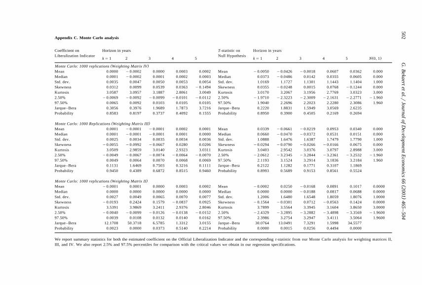
()
G.B
ekaertetal.r
JournalofD
eÕelopm
entEconom
ics66
2001465
–504
502
Appendix C. Monte Carlo analysis
Coefficient on Horizon in years T-statistic on Horizon in yearsLiberalization Indicator Null Hypothesis Ž .ks 1 2 3 4 5 ks 1 2 3 4 5 N 0, 1
( )Monte Carlo: 1000 replications Weighting Matrix IVMean 0.0000 y0.0002 0.0000 0.0003 0.0002 Mean y0.0050 y0.0426 y0.0018 0.0607 0.0362 0.000Median 0.0001 y0.0002 0.0001 0.0002 0.0003 Median 0.0373 y0.0486 0.0142 0.0355 0.0605 0.000Std. dev. 0.0035 0.0047 0.0050 0.0053 0.0054 Std. dev. 1.0169 1.1727 1.1301 1.1443 1.1404 1.000Skewness 0.0312 0.0099 0.0539 0.0363 y0.1494 Skewness 0.0355 y0.0248 0.0015 0.0768 y0.1244 0.000Kurtosis 3.0587 3.0957 3.1887 2.8061 3.0049 Kurtosis 3.0170 3.2067 3.1956 2.7769 3.0323 3.0002.50% y0.0069 y0.0092 y0.0099 y0.0101 y0.0112 2.50% y1.9710 y2.3223 y2.3009 y2.1631 y2.2771 y1.96097.50% 0.0065 0.0092 0.0103 0.0105 0.0105 97.50% 1.9040 2.2696 2.2023 2.2280 2.3086 1.960Jarque–Bera 0.3056 0.3976 1.9689 1.7873 3.7216 Jarque–Bera 0.2220 1.8831 1.5949 3.0569 2.6235Probability 0.8583 0.8197 0.3737 0.4092 0.1555 Probability 0.8950 0.3900 0.4505 0.2169 0.2694
( )Monte Carlo: 1000 Replications Weighting Matrix IIIMean 0.0001 y0.0001 y0.0001 0.0002 0.0001 Mean 0.0339 y0.0661 y0.0219 0.0953 0.0340 0.000Median 0.0001 y0.0001 y0.0001 0.0001 0.0000 Median 0.0660 y0.0470 y0.0372 0.0531 0.0151 0.000Std. dev. 0.0025 0.0034 0.0035 0.0034 0.0036 Std. dev. 1.0888 1.6476 1.6387 1.7479 1.7790 1.000Skewness y0.0055 y0.0992 y0.0667 0.0280 0.0206 Skewness y0.0294 y0.0790 y0.0266 y0.0166 0.0675 0.000Kurtosis 3.0509 2.9859 3.0140 2.9323 3.0311 Kurtosis 3.0403 2.9542 3.0376 3.0797 2.8988 3.0002.50% y0.0049 y0.0067 y0.0074 y0.0064 y0.0070 2.50% y2.0612 y3.2345 y3.2844 y3.2361 y3.2532 y1.96097.50% 0.0049 0.0064 0.0070 0.0068 0.0069 97.50% 2.1193 3.1524 3.2914 3.1836 3.2184 1.960Jarque–Bera 0.1131 1.6469 0.7503 0.3216 0.1111 Jarque–Bera 0.2122 1.1282 0.1771 0.3107 1.1869Probability 0.9450 0.4389 0.6872 0.8515 0.9460 Probability 0.8993 0.5689 0.9153 0.8561 0.5524
( )Monte Carlo: 1000 replications Weighting Matrix IIMean y0.0001 0.0001 0.0000 0.0003 0.0002 Mean y0.0002 0.0250 y0.0168 0.0891 0.1017 0.0000Median 0.0000 0.0000 0.0000 0.0000 0.0000 Median 0.0000 0.0000 y0.0188 0.0817 0.0688 0.0000Std. dev. 0.0027 0.0049 0.0065 0.0070 0.0077 Std. dev. 1.2006 1.6480 1.6548 1.8059 1.8076 1.0000Skewness y0.0193 0.2424 0.1579 y0.0837 0.0925 Skewness y0.1564 y0.0301 0.0712 y0.0563 0.1424 0.0000Kurtosis 3.5391 3.9869 3.2411 2.9376 2.8046 Kurtosis 3.7899 3.5564 3.3945 3.1604 3.8650 3.00002.50% y0.0040 y0.0099 y0.0126 y0.0138 y0.0152 2.50% y2.4329 y3.2895 y3.2882 y3.4898 y3.3569 y1.960097.50% 0.0039 0.0108 0.0132 0.0140 0.0162 97.50% 2.3986 3.2754 3.2947 3.4111 3.5064 1.9600Jarque–Bera 12.1708 50.3718 6.5785 1.3312 3.0155 Jarque–Bera 30.0764 13.0491 7.3291 1.5998 34.5577Probability 0.0023 0.0000 0.0373 0.5140 0.2214 Probability 0.0000 0.0015 0.0256 0.4494 0.0000
We report summary statistics for both the estimated coefficient on the Official Liberalization Indicator and the corresponding t-statistic from our Monte Carlo analysis for weighting matrices II,III, and IV. We also report 2.5% and 97.5% percentiles for comparison with the critical values we obtain in our regression specifications.
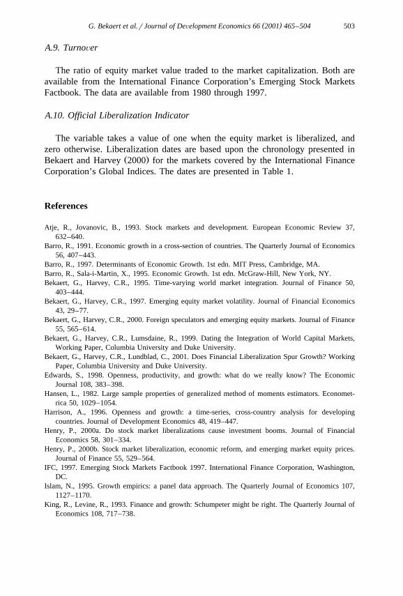
( )G. Bekaert et al.rJournal of DeÕelopment Economics 66 2001 465–504 503
A.9. TurnoÕer
The ratio of equity market value traded to the market capitalization. Both areavailable from the International Finance Corporation’s Emerging Stock MarketsFactbook. The data are available from 1980 through 1997.
A.10. Official Liberalization Indicator
The variable takes a value of one when the equity market is liberalized, andzero otherwise. Liberalization dates are based upon the chronology presented in
Ž .Bekaert and Harvey 2000 for the markets covered by the International FinanceCorporation’s Global Indices. The dates are presented in Table 1.
References
Atje, R., Jovanovic, B., 1993. Stock markets and development. European Economic Review 37,632–640.
Barro, R., 1991. Economic growth in a cross-section of countries. The Quarterly Journal of Economics56, 407–443.
Barro, R., 1997. Determinants of Economic Growth. 1st edn. MIT Press, Cambridge, MA.Barro, R., Sala-i-Martin, X., 1995. Economic Growth. 1st edn. McGraw-Hill, New York, NY.Bekaert, G., Harvey, C.R., 1995. Time-varying world market integration. Journal of Finance 50,
403–444.Bekaert, G., Harvey, C.R., 1997. Emerging equity market volatility. Journal of Financial Economics
43, 29–77.Bekaert, G., Harvey, C.R., 2000. Foreign speculators and emerging equity markets. Journal of Finance
55, 565–614.Bekaert, G., Harvey, C.R., Lumsdaine, R., 1999. Dating the Integration of World Capital Markets,
Working Paper, Columbia University and Duke University.Bekaert, G., Harvey, C.R., Lundblad, C., 2001. Does Financial Liberalization Spur Growth? Working
Paper, Columbia University and Duke University.Edwards, S., 1998. Openness, productivity, and growth: what do we really know? The Economic
Journal 108, 383–398.Hansen, L., 1982. Large sample properties of generalized method of moments estimators. Economet-
rica 50, 1029–1054.Harrison, A., 1996. Openness and growth: a time-series, cross-country analysis for developing
countries. Journal of Development Economics 48, 419–447.Henry, P., 2000a. Do stock market liberalizations cause investment booms. Journal of Financial
Economics 58, 301–334.Henry, P., 2000b. Stock market liberalization, economic reform, and emerging market equity prices.
Journal of Finance 55, 529–564.IFC, 1997. Emerging Stock Markets Factbook 1997. International Finance Corporation, Washington,
DC.Islam, N., 1995. Growth empirics: a panel data approach. The Quarterly Journal of Economics 107,
1127–1170.King, R., Levine, R., 1993. Finance and growth: Schumpeter might be right. The Quarterly Journal of
Economics 108, 717–738.

( )G. Bekaert et al.rJournal of DeÕelopment Economics 66 2001 465–504504
Levine, R., Renelt, D., 1992. A sensitivity analysis of cross-country growth regressions. The AmericanEconomic Review 82, 942–963.
Levine, R., Zervos, S., 1998. Stock markets, banks, and economic growth. The American EconomicReview 88, 537–558.
Newey, W., West, K., 1987. A simple, positive semi-definite, heteroskedasticity and autocorrelationconsistent covariance matrix. Econometrica 55, 703–708.
Rodrik, D., 1999. Determinants of Economic Growth. Overseas Development Council, Washington,DC.