Embed Size (px)
Citation preview

Policy Research Working Paper 5961
Emerging Economies in the 2000s
Real Decoupling and Financial Recoupling
Eduardo Levy YeyatiTomas Williams
The World BankLatin American and Caribbean RegionOffice of the Chief EconomisFebruary 2012
WPS5961 P
ublic
Dis
clos
ure
Aut
horiz
edP
ublic
Dis
clos
ure
Aut
horiz
edP
ublic
Dis
clos
ure
Aut
horiz
edP
ublic
Dis
clos
ure
Aut
horiz
edP
ublic
Dis
clos
ure
Aut
horiz
edP
ublic
Dis
clos
ure
Aut
horiz
edP
ublic
Dis
clos
ure
Aut
horiz
edP
ublic
Dis
clos
ure
Aut
horiz
ed

Produced by the Research Support Team
Abstract
The Policy Research Working Paper Series disseminates the findings of work in progress to encourage the exchange of ideas about development issues. An objective of the series is to get the findings out quickly, even if the presentations are less than fully polished. The papers carry the names of the authors and should be cited accordingly. The findings, interpretations, and conclusions expressed in this paper are entirely those of the authors. They do not necessarily represent the views of the International Bank for Reconstruction and Development/World Bank and its affiliated organizations, or those of the Executive Directors of the World Bank or the governments they represent.
Policy Research Working Paper 5961
The paper documents an intriguing development in the emerging world in the 2000s: a decoupling from the business cycle of advanced countries, combined with the strengthening of the co-movements in the main emerging market assets that predates the synchronized sell-off during the crisis. In addition, the paper tests the hypothesis that financial globalization, to the extent that it creates a common, global investor base for emerging markets, could lead to a tighter asset correlation despite
This paper is a product of the Office of the Chief Economist, Latin American and Caribbean Region. It is part of a larger effort by the World Bank to provide open access to its research and make a contribution to development policy discussions around the world. Policy Research Working Papers are also posted on the Web at http://econ.worldbank.org. The author may be contacted at [email protected].
the weaker economic ties. While an examination of the impact of alternative financial globalization proxies does not yield conclusive results, a closer look at global emerging market equity and bond funds shows that the latter indeed foster financial recoupling during downturns, reflecting the fact that they trade near their respective benchmarks and respond to withdrawals by liquidating holdings across the board.

Decoupling and recoupling
1 !
Emerging economies in the 2000s:
Real decoupling and financial recoupling
Eduardo Levy Yeyati1
Universidad Torcuato Di Tella
Tomas Williams
Barcelona GSE
Abstract
The paper documents an intriguing development in the emerging world in the 2000s: a
decoupling from the business cycle of advanced countries, combined with the strengthening of
the co-movements in the main emerging market assets that predates the synchronized sell-off
during the crisis. In addition, the paper tests the hypothesis that financial globalization, to the
extent that it creates a common, global investor base for emerging markets, could lead to a
tighter asset correlation despite the weaker economic ties. While an examination of the impact of
alternative financial globalization proxies does not yield conclusive results, a closer look at
global emerging market equity and bond funds shows that the latter indeed foster financial
recoupling during downturns, reflecting the fact that they trade near their respective benchmarks
and respond to withdrawals by liquidating holdings across the board.
1 We would like to thank Mariana Barrera for outstanding research assistance, and seminar participants at the World Bank, Brookings Institution, the Geneva Graduate Institute and Universidad de San Andres for their useful comments. Tatiana Didier kindly provided the data used in some of the tests in the paper. We would also like to thank The World Bank´s CEO for financial support for this research agenda, as part of the 2011 flagship report on Latin American financial markets. The usual disclaimers apply.

Decoupling and recoupling
2 !
1. Introduction
Emerging markets (EM) advocates often emphasize their newly gained resilience to external
shocks. Resilience, however, can be interpreted in several ways. In particular, it is expected to
manifest differently according to whether it refers to economic performance, market
interdependence, or the link between markets and economic activity. In this paper, we revisit the
debate surrounding the different varieties of EM decoupling to document the recent behavior (in
both the pre-crisis bonanza and the turbulent crisis period) on these three fronts, discuss the
economic factors underlying the specific patterns in each case, and draw market and policy
implications from these findings.
In particular, we examine decoupling: (i) in the traditional sense, namely, business cycle
synchronicity and sensitivity to the world economy (real decoupling); and (ii) as cross-market
financial interdependence (financial decoupling), in the sense of the “betas” of EM credit, equity
and currency returns to returns on the global market portfolio, as well as within-EM betas (a
typical feature of the 1990s); Finally, we center the debate around EM financial integration to the
world (as the deepening of financial capital inflows) and its impact on financial ties of EM assets
to those in the developed world.
The discussion is centered on EM assets. More specifically, we look at a sample of countries
that represents what is usually labeled as emerging markets in the financial industry, following
the Morgan Stanly Capital Index benchmark (MSCI) for individual countries and groups of
countries, and focus our analysis on equity and, to a lesser extent, currency and hard currency
sovereign bonds. As a comparison group, we include in the study a sample of advanced markets
detailed in the Appendix.
We find that: (i) on the real front, rather than actually decoupling from the world, EM have
diversified away from the US and the euro zone into emerging Asia (through international trade
and the growing economic importance of China); (ii) on the market front, despite the real
decoupling, the co-movement between EM and global assets (as measured by the EM betas to
developed markets return) has risen in the late 2000s, even before the 2008-2009 crisis.
Why has real decoupling not provided more “room” for assets from fundamentally sound EM
to decouple as well? A priori, financial globalization (FG), to the extent that it internationalized

Decoupling and recoupling
3 !
EM´s investor base, could be the explanation for the tighter co-movement (as suggested, e.g., by
Didier et al., 2010 for a broader country sample). While a closer look at the impact of traditional
FG proxies yields a negative result, capital flows from global and global emerging equity and
bond funds indeed foster financial recoupling during downturns, reflecting the fact that they
trade near their respective benchmarks and respond to withdrawals by liquidating holdings across
the board.
The paper is organized as follows. Section 2 compares alternative definitions of EM. Section
3 examines real decoupling. Section 4 looks at credit, equity and currency betas over time to
document the financial recouping in recent years. Section 5 explores the link between EM betas
and alternative measures of FG. Finally, section 6 summarizes the results and concludes.
2. A map of the emerging world
While the buzzword “emerging”, alternatively attached to markets and economies, has been
around for 30 years, the connotation of the term has changed dramatically over time.2 From an
empirical perspective, emerging markets came into their own as an asset class only in the early
1990s, as the post-Bretton Woods financial globalization trend that consolidated in advanced
countries in the 1980s moved on to the developing world.3 Therefore, evaluating their
performance starting in the early 1980s (when many EM did not even exist as national entities)
could be greatly misleading.
The fact that “emerging” often denotes financial and economic aspects interchangeably opens
the door for some divergence in the way the EM group is populated. There are several criteria
according to which emerging economies can be identified and classified including: geography
(acknowledging the incidence of regional ties) as in the many regional EM equity indexes;
economic development (typically proxied by national income); and market infrastructure (often
associated with one specific market), as in the FTSE classification, or economic size and
2 As the story goes, the IFC staffer Antoine van Agtmael coined the term in 1981 to elude the negative connotation of the then popular “third world” label, at a time at which there was practically no foreign portfolio investment in those markets. 3 Obstfled and Taylor (2002) provide a useful historical perspective.

Decoupling and recoupling
4 !
geopolitical influence, as in the BRIC category4 Moreover, the conventional (but often disputed)
growth convergence view would suggest a negative correlation between growth upside and income
(often used to screen advanced from emerging economies). A casual examination of the link
between per capita GDP and IMF growth forecasts points in the same direction (Figure 1).
At any rate, a quick glance at different EM groupings reveals mostly coincidences in the broad
breakdown, but some important differences within the EM tier (Table 1). Hong Kong SAR, China;
Israel; Singapore; and sometimes South Korea are regarded as advanced based on income and
stock market development, although they are still treated as emerging for fixed income industry
analysts. On the other corner, Chile’s low income and less-than-stellar equity markets understate
its economic progress and its developed bond market.
We do not intend to settle this semantic question in this series. Rather, as shown in Table 1,
we use here a standard broad EM grouping that could change due to data availability in some
sections. In addition, for some exercises we look at a group of advanced markets as benchmark.
3. Real decoupling and growth convergence
One of the arguments often used by emerging markets (EM) advocates highlights that, because
of the natural diversification in the sources of economic growth (due to increased openness and
globalization) or because of structural changes and policy improvements, emerging economies have
become more resilient to changes in the global context (see. E.g., The Economist, 2009). If, in the
1990s, whenever the world caught a cold EM got pneumonia, past financial crises would have
immunized emerging economies so that, if anything, when in 2008 the G7 got pneumonia, EM just
got a cold.
However, this popular decoupling argument is both less straightforward and more controversial
than what its narrative suggests. For starters, common measures of decoupling tell a different story.
On the empirical side, the share of the growth variability explained by the first principal
component of quarterly growth for a group of developed and EM economies has increased sharply
4 Along the same lines, newly industrialized countries (NICs) is a category between developed and developing countries, which includes Brazil, the People's Republic of China, India, Malaysia, Mexico, Philippines, South Africa, Thailand and Turkey.

Decoupling and recoupling
5 !
in the 2000s (Figure 2), and the same (albeit smaller) increases can be found by looking at cross-
country correlations (Rose, 2009).
Interestingly, the correlation of business cycles, the measure of decoupling that became
standard in the economic literature, mixes sensitivity and amplitude. For example, the correlation
between EM and G7 output, !!"!!! ! !!"!!! !!"!!!!
can increase with the beta between the two
as well as with the ratio of output volatilities. Thus, the Great Moderation of the pre-crisis period
(to the extent that it reduced !!!) and a home-grown EM crisis (to the extent that it rises !!")
could increase the correlation even if the beta between the two countries remains unaltered.5 On the
other hand, pure synchronicity measures (see, e.g., Mink and de Haan, 2007), while closer to the
canonical definition of decoupling, are silent about the economic relevance of the connection.
At any rate, results using these measures are rather disappointing, as evidence of decoupling
is seldom found: if anything, the 2000s seems to have witnessed an increase in the correlations of
EM and G7 cycles (Figure 3).6 By contrast, with a few exceptions, EM have been exhibiting
growth outperformance that, according to most forecasts, will continue in the next few years
(Figure 4).
Sensitivity to global shocks is a key aspect of decoupling from the perspective of the risk
associated to EM assets, where we care as much about how much EM volatility would result
from a given global shock as the timing of the response. It is also critical in the context of the
new EM debate (namely, the degree of progress the main emerging economies have made since
the financially challenging 1990s). After all, if a global crisis, by definition, hits everybody, EM
resilience and quality cannot be judged by the fact that they responded to last year’s global
shock, but rather by how much and for how long. The natural way to test whether EM sensitivity
to global growth has declined over the years is to regress EM growth on G7 growth and evaluate
how the coefficients (EM growth “betas” to the developed world) have evolved since the
inception of EM as an asset class in 1993. Splitting the sample in an early (1993-99) and a late
5The same caveat applies to a comparison of the explanatory power of time-varying global factors based on the R2 (as in Kose et al., 2008) since R2
EM,G7 = !2 EM,G7.
6 HP filtered output growth yields remarkably similar results. Rose (2009) reports and discusses different versions of this exercise. Walti (2009) applies Mink and de Haan’s (2007) synchronicity measure based on the product of output gaps: (gapi/|gapi|)*(gapj/ |gapj|) which is equal to sign (gapi * gapj) *1, for the two-country or two-region case.

Decoupling and recoupling
6 !
(2000-Q3 2010) period, and assuming for simplicity that trend growth remained stable within
each sub-period, the specification is simple enough:
!!" !"!!" !! ! !!!!" !"!!!!! ! !!!!" !"!!!!! ! !!"#$ ! !!!!" !"!!!!"#!! ! !!!!" !"!!!!"#!! ! !!"#$
(1)
a regression of the annual q/q growth rate of country i’s cyclical output (relative to a log linear
GDP trend) on the G7 and Chinese cycles, based on quarterly data, identifying the late period
(2001-Q3 2010) with an interacting dummy. In passing, such a specification also allows us to
estimate the long-term growth convergence (the EM “alphas”) as the constant of the regression.
Note that we deliberately exclude China from the EM sample. For sheer size and growth
dynamics, China represents a class in itself that, if grouped with other EM, could bias the
conclusions of this exercise (as it does, most notably, in the typical analysis of EM aggregate
output). Indeed, it remains a global driver that should be treated as an additional exogenous force
behind EM growth and, thus, be included as an additional control, as we do here.
Table 2 summarizes the results. The first thing to note is the fact that emerging economies
display mostly “positive alphas” relative to the G7 group: a median 2.5% growth differential
(Column 4) per year over the whole period, roughly in line with the back-of-the-envelope
illustration in Figure 5. Is the elusive growth convergence finally materializing in the emerging
world? While it is still far too early to judge, at first glance their relative growth performance is
not inconsistent with the convergence view, not only vis a vis developed economies but, most
strikingly, within the emerging group as well (Figure 4).
Regarding decoupling per se, in the traditional specification in which global growth is
represented by the G7, the EM betas appear stable and high. In other words, there seems to have
been no decoupling in the past decade, a finding mostly in line with the results in the recent
economic literature (Rose, 2009; Wälti, 2009).
However, the data paint a different picture once we include China as a separate control: the
explanatory power of the G7 clearly diminishes in the latest period, at the expense of the Chinese
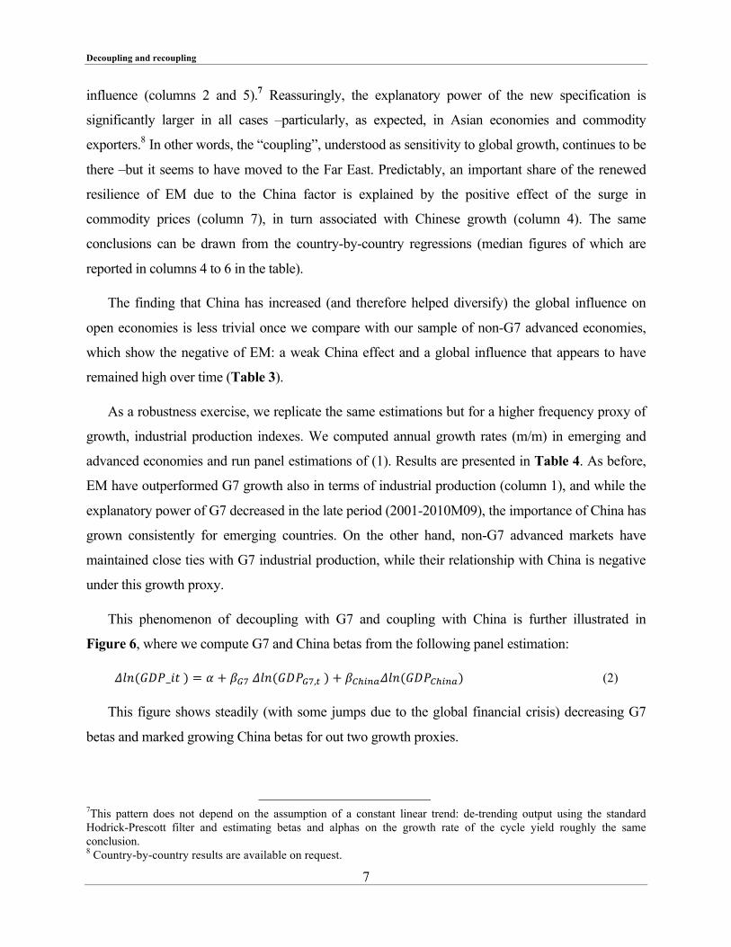
Decoupling and recoupling
7 !
influence (columns 2 and 5).7 Reassuringly, the explanatory power of the new specification is
significantly larger in all cases –particularly, as expected, in Asian economies and commodity
exporters.8 In other words, the “coupling”, understood as sensitivity to global growth, continues to be
there –but it seems to have moved to the Far East. Predictably, an important share of the renewed
resilience of EM due to the China factor is explained by the positive effect of the surge in
commodity prices (column 7), in turn associated with Chinese growth (column 4). The same
conclusions can be drawn from the country-by-country regressions (median figures of which are
reported in columns 4 to 6 in the table).
The finding that China has increased (and therefore helped diversify) the global influence on
open economies is less trivial once we compare with our sample of non-G7 advanced economies,
which show the negative of EM: a weak China effect and a global influence that appears to have
remained high over time (Table 3).
As a robustness exercise, we replicate the same estimations but for a higher frequency proxy of
growth, industrial production indexes. We computed annual growth rates (m/m) in emerging and
advanced economies and run panel estimations of (1). Results are presented in Table 4. As before,
EM have outperformed G7 growth also in terms of industrial production (column 1), and while the
explanatory power of G7 decreased in the late period (2001-2010M09), the importance of China has
grown consistently for emerging countries. On the other hand, non-G7 advanced markets have
maintained close ties with G7 industrial production, while their relationship with China is negative
under this growth proxy.
This phenomenon of decoupling with G7 and coupling with China is further illustrated in
Figure 6, where we compute G7 and China betas from the following panel estimation:
!"#!!"#!!"!! ! ! ! !!!!!"#!!"!!!!!!! ! !!!!"#!"#!!"!!!!"#! (2)
This figure shows steadily (with some jumps due to the global financial crisis) decreasing G7
betas and marked growing China betas for out two growth proxies.
7This pattern does not depend on the assumption of a constant linear trend: de-trending output using the standard Hodrick-Prescott filter and estimating betas and alphas on the growth rate of the cycle yield roughly the same conclusion. 8 Country-by-country results are available on request.

Decoupling and recoupling
8 !
Our results in this section are based upon the assumption that China is an independent engine of
growth for EM, and its relationship with G7 growth is minor. As a way to illustrate the fact that
China has been going its own way is to compute the principal components of growth for a G8 group
comprised of the G7 + China. As the weights of the first two PC indicate (Figure 7), Chinese
growth is captured by the second component, orthogonal to the first component that explains other
G7, with Japan sitting halfway between other advanced economies and China.
This is further confirmed by country regressions of growth against the first two principal
components (Figure 8): G7 countries are largely explained by the first one, China by the second
one. In other words, we can safely say that, in the period under study, China represented an
independent (and, based on Table 2, quite influential) new engine of emerging market growth.
4. Financial recoupling
A common misperception among EM advocates and practitioners is the idea that the newly
gained policy autonomy and macroeconomic resilience to external shocks have enhanced the
importance of a country’s fundamentals as drivers of asset performance – a view typically
contradicted by the data, which reveal a steady influence of global factors and persistently high
betas.9
As before, we proceed in two steps. First, we examine whether the degree of assets price co-
movement estimating the share of time variability explained by the first principal component
(PC1), this computed based on EM asset performance, and regress country-specific equity and
FX returns, and CDS spread changes, on the PC1 constructed for each EM asset class, to get the
average R2. As can be seen in Figure 9, the portion explain by PC1 is considerable in both
cases, and has been growing over time (even before the 2008-2009 selloff).
In turn, PC1 is highly correlated with global factors, indicating that most of the co-movement
displayed by EM assets comes from global influences or globally synchronized shocks (Table
5).
9 Much as in the case of real decoupling discussed above, the drawbacks of using standard correlations to estimate market interdependence have been repeatedly highlighted in the finance literature, most notably Forbes and Rigobon (2002).

Decoupling and recoupling
9 !
Have the betas of EM assets to global assets come down in recent years? This is readily
illustrated by a back-of-the-envelope estimation of betas relative to standard global proxies for
each of the relevant markets. Specifically, we run country-by-country regressions of monthly log
changes in MSCI country equity indexes, exchange rates and credit spreads on log changes in the
S&P 500, Broad Dollar Index, and US, respectively, to estimate alphas and betas as the ordinate
and the coefficient from the regressions.10 We focus on two time periods: early (2000-2004) and
late (2005-2010), and we split the latter into a tranquil period (2005-2008M02) and a longer late
period including the crisis (2005-2010). We replicate the exercise for quarterly and annual
changes to examine whether longer time horizons enhance the effect of fundamentals at the
expense of global markets.
As Figure 10 clearly shows, betas have remained persistently high in the second half of the
2000s, even as we lower the sampling frequency to allow for short-term co-movement to
dissipate (Table 6 report the group means and medians). Equities betas have remained close to 1,
while credit betas (sovereign bond spreads vis a vis high yield corporate spreads in advance
countries) and exchange rate betas have generally increased. Table 6 also shows that high betas
are not a result of the global financial crisis, as the pre-crisis period (2005-2008M02) presents
betas in EM’s assets that are greater or equal to betas during the early 2000s. Interestingly, this
change in global betas is not idiosyncratic to EM, as it also applies to the advanced economies in
our sample. However, financial recoupling in these economies have less strength than in EM,
and is particularly found in equity markets and to a less extent in FX markets.11
To further investigate financial recoupling we performed panel estimations instead of
country-by-country regressions of log changes in EM assets against global assets. Results are
summarized in Table 7. For the three assets under consideration, we observe financial
recoupling during the late 2000s even when we remove the crisis period (2008M03-2009M03).12
Our results are also in line with Dooley and Hutchinson (2009). In their study, they conclude that
emerging markets experienced greater financial transmission during the worst period of the
10 We use the S&P, Broad Dollar Index and US HY instead of broader global indexes to be able to estimate alphas and betas for the advanced markets we used for comparison in the previous piece of this series. Estimating equity betas to the global MSCI yields comparable results. We choose MSCI equity indexes to local stock market indexes to concentrate on the more liquid, globally traded stocks used in cross-border operations. 11 Sovereign debt in advanced economies is largely domestic and denominated in local currency, hence not directly comparable with EM credit. 12 Financial recoupling is also present with semi-annual and annual log changes. These results are not presented for brevity but are available upon request.

Decoupling and recoupling
10 !
global financial crisis (i.e. betas increased even more during this financial turmoil). However,
Dooley and Hutchinson (2009) analyze the financial recoupling-decoupling hypothesis
comparing the period going from early 2007 to summer 2008 with the Lehman and post-Lehman
period of the crisis.13 In here, we go a little further, by findng that during the 2000s EM have not
decouple, financially speaking, from global assets. Furthermore, our evidence points towards a
financial recoupling during this period, that was taking place even before the global financial
crisis of 2008/2009.
5. Is Financial recoupling the result of financial globalization?
Why have market betas to global drivers remained so high despite the more diversified
economic pattern displayed by EM in the 2000s? In principle, stable to higher betas could be seen as
the natural consequence of financial globalization, to the extent that the latter tends to increase the
global nature of EM´s investor base, thereby making it more homogeneous. As the global investors
increasingly participate in emerging markets (Figure 11), the importance of global factors coming
from the developed world increases at the expense of within-EM factors that represented the typical
source of contagion in the 1990s.
On the other hand, in the late 2000s, emerging assets prices have exhibited a clear high-beta,
high-alpha pattern relative to global assets (Figure 12); namely, a tightly correlated oscillation
around clearly diverging trends (in line with results in Table 7).14
In this section, we explore whether this pattern (particularly, the high beta) is related to (or is a
consequence of) financial globalization. To do that, we focus on the three EM assets classes
previously discussed: credit, currencies and equity.
13 As we do, they analyze equity, debt and FX markets in EM. They use daily data and analyze whether news emanating from the US had more or less impact comparing these two phases of the US subprime crisis. 14 By alphas and betas we refer to the coefficients of a simple regression of return of the EM asset on the return of a comparable market portfolio (both in excess of the risk free rate), which in turn are associated, respectively, with (diversifiable) idiosyncratic and (non diversifiable) systemic returns.
Decoupling and recoupling
11 !
a. Financial globalization: What do we talk about?15
Despite being the subject of a rich and growing literature, the concept of financial
globalization has been defined in various, often-uncorrelated ways in the academic work. As a
result, assessing a country’s integration with international financial markets remains a
complicated and controversial task.
Today it is well accepted that the extent to which globalization affects asset prices and, more
generally, is related to the actual intensity and sensitivity of cross-border flows, regardless of
existing controls and restrictions usually at the core of de jure globalization measures.16 For
example, many tightly regulated economies are the recipients and sources of important capital
flows (and are therefore financially globalized), whereas other control-free economies are
shunned by international investors and, as a result, are isolated from global market swings and
trends. In turn, the empirical literature typically measured de facto globalization as the ratio of
foreign asset positions (relative price-adjusted cumulative balance of payments flows) to GDP,
as in Lane and Milessi-Ferreti (2006 and 2007; henceforth, LMF).17
It should be noted, however, that the stock size of cross border holdings, while probably a
good indicator of geographical diversification and international risk sharing, may not be the best
summary statistic of de facto FG in the traditional sense of capital mobility and international
arbitrage, since important gross flows in and out of a country over a given year are perfectly
consistent with a relatively small net –as well as with small cumulative flows over longer
periods. As a result, to the extent that foreign asset holdings largely reflect cumulative flows,
intense flows could be consistent with a limited geographical diversification of assets and
liabilities. Conversely, the existence of large foreign asset holdings (for example, as a result of
capital flight) does not necessarily imply frequent rebalancing and cross-market arbitrage. Thus,
15 This section borrows from Levy Yeyati and Williams (2010). 16 The literature generally distinguishes between de jure and de facto financial globalization (Kose, Prassad, Rogoff, Wei, 2009): where the former is based on regulations, restrictions and controls over capital flows and asset ownership, the latter is related to the intensity of capital flows and cross-market correlation and arbitrage. 17Kraay, Loayza and Ventura (2005) report a similar dataset on country´s asset positions. An alternative approach to FG relies on price convergence, an application of the Law of one Price to financial markets. Measures within this group point at transaction costs and regulation that inhibit market arbitrage, and usually compare prices of identical or similar assets trading in different markets. On this, see Levy Yeyati, Schmukler and Van Horen (2008) and references therein. LMF and the Chinn-Ito index are the de facto and de jure measures of choice in recent work on determinants and implications of FG (see, i.a., Kose, Prasad, Taylor, 2009 and Rodrik, and A. Subramanian, 2009).

Decoupling and recoupling
12 !
depending on the specific issue at hand, stock holdings, capital flows or both may prove
informative.
In addition, the investor behind a particular flow may also be relevant to understand FG. For
example, a passive buy and hold portfolio investor may behave closer to real investors (FDI),
with limited turnover (flows) for a given holding. By contrast, institutional or professional
investors would tend to be more sensitive to expected return differentials, with both a larger
turnover and a bigger impact in terms of price action its correlation across markets and with
respect to economic fundamentals. Global mutual funds are a case in point in this regard. While,
as a subset of cross-border holdings, they are generally a poorer proxy than other more
comprehensive measures, they may shed some additional light on the role of the international
investor as a financial transmission channel. To the extent that these funds tend to keep close to
their benchmarks, they may introduce an additional source of market co-movement, particularly
in the event of sharp swings in global risk aversion (when contributions and redemptions lead to
purchases and sales in all markets at the same time).
In this light, we try to analyze different measures of de facto FG by their advantages and
disadvantages of using them as proxies of financial globalization in emerging markets. More
precisely, we look at two different sources: (i) US Treasury’s TIC monthly survey data on the
market value of sales and purchases, and stocks holdings of foreign securities by US-domiciled
investors (by the market where the security is issued); and (ii) EPFR’s monthly data on global
fund flows and assets under management (AUM) (by the issuing country).
In our study, we are interested in asset prices on a monthly basis, and to address whether
financial recoupling (or greater financial contagion) in the late 2000s was associated with
financial globalization. At first sight, frequency and length problems arise with both Lane and
Milesi-Ferretti’s (2007) and BoP statistics. Annual foreign stocks from LMF are available until
2007, and are inadequate to analyze asset prices and financial globalization in the late 2000s,
particularly at times when the global financial crisis may have significantly modified gross
foreign asset positions. On the other hand, while updated BoP statistics are available, they are
usually reported on a quarterly or an annual basis. To study whether greater flow intensity
generates the monthly asset correlation behind financial recoupling, we need higher frequency
data such as the U.S. Treasury’s TIC and EPFR data.

Decoupling and recoupling
13 !
TIC data collect cross-border holdings of securities measured at market value through
security-level surveys (that is, information is reported separately for each security) that conflate
data from custodians, issuers, and investors. As the data is collected by the US Treasury, it
comprises transactions between U.S. residents and counterparties located outside the United
States involving six types of securities, including four domestic (U.S. Treasury bonds and notes,
bonds of U.S. government corporations and federally-sponsored agencies, U.S. corporate and
other bonds, and U.S. corporate and other stocks) and two foreign (foreign bonds and foreign
stocks). We compute liability flows coming from the US as the difference between gross
purchases and gross sales of foreign securities by US residents. In turn, EPFR data report the
fund net flow to individual emerging economies, as well as the assets under management (AUM)
by country.
There are differences between TIC and EPFR data. On the one hand, unlike annual TIC data,
EPFR data is available at monthly (and, for a subset of funds, weekly) frequency. More
importantly, the simple within-country correlation between both flow measures is rather low
(Table 8), reflecting the distinct behavioral pattern between both sources: as we stated above,
global funds tend to keep close to their benchmark, inducing correlation (as a result of global
swings in risk appetite and exposure) and possibly exacerbating financial contagion, while the
average TIC respondent would tend to trace less and to exhibit a more selective sensitivity to
relative price changes.
A degree of complexity in the measurement of de facto FG is introduced by the
normalization. On the one hand, normalization by the (US dollar) GDP looks natural for issues
related with the country´s wealth diversification away from domestic shocks (and exposure to
external shocks). On the other hand, normalization by local market capitalization seems to be
more appropriate when assessing cross-border flows as a source of price volatility and
international contagion. The differences are not trivial: as we show in a companion paper (Levy
Yeyati and Williams (2010)), whereas in the 2000s globalization in EM remained stable in terms
of foreign market participation, it grew in terms of GDP reflecting the valuation effect of the
equity rally before and after the 2008 slump. To avoid capturing these spurious price effects,
here we normalize equity liability flows by local equity market capitalization and debt liability
flows by the total outstanding debt of the recipient country.

Decoupling and recoupling
14 !
Yet another source of concern arises from the less-than-perfect correspondence between
stocks holdings and the volume of flows. Levy Yeyati and Williams (2010) report that the
relationship between the size (that is, the absolute value) of this year´s flows and end-of-last-
year´s holdings (based on holdings data from LMF and BoP flow data) is significant for EM
equity and FDI but not for debt instruments. However, using EPFR´s global fund data, they find
that the link is significant and stronger for both equity and debt instruments. At any rate, to the
extent that flows are only imperfectly characterized by initial holdings, it is useful to proxy
globalization both by foreign liability stock (as is typically done in the literature) and flow ratios.
b. Globalization, benchmarking and financial recoupling
Does foreign participation increase the market betas to global returns? Does FG amplify the
response of cross-border flows and asset prices in times of global turmoil? A first look at the data
appears to contradict this hypothesis. Although in principle there seems to be a significant link
between holdings and betas (Didier et al, 2010) a closer look reveals that it is entirely accounted
for by the group of non-EM developing frontier markets.18
Table 9 illustrates the point. The first column reproduces the main result in Didier et al.
(2010), which tries to explain the financial channel behind the large post-Lehman betas,
controlling for market moves with time dummies: US holdings from TIC data do not explain but
significantly amplify the sensitivity of EM equity to global returns (measured from a regression
of the monthly change in the local stock market index against monthly returns on the S&P 500).
However, as the next two columns reveal, the result is entirely driven by frontier markets: US
equity holdings do not change significantly the impact of S&P returns on equity returns in either
developed or emerging economies. The same is true when, in the second half of the table, we
drop the Lehman interaction and replace time dummies by S&P returns (a specification closer to
our focus on market betas, here assumed to be a linear function of US holdings). Given that
flows and stocks are not always tightly correlated (and that, ultimately, it is the flow that
influences the price action in these markets): does the test change when we use the volume (that
is, the absolute value) of TIC equity liability flows? According to the results in column 9, the
18 Tatiana Didier kindly provided the data for this table.
Decoupling and recoupling
15 !
answer is no –not surprisingly, since equity inflows tend to be closely correlated with foreign
equity holdings (Levy Yeyati and Williams, 2011).
Figure 13 presents a graphical illustration of these results by plotting country-by-country
equity betas against US holdings, and showing how, unlike in the case of frontier markets, the
expected positive link between betas and FG fails to materialize.
As noted, there are important difference between the average international investor and the
professional asset manager, not least of them the fact that the latter are usually benchmarked,
which limits their decisions to small deviations from the market weights, forcing them to
purchase or liquidate in all markets proportionally in the event of massive allocations or
withdrawals from the asset class. In other word, global flows may explain the growing
correlation of EM assets with US markets better than the holdings of the average U.S. resident
investor.
With that in mind, in Table 10 we replicate the exercise in column 9 of Table 9 using EPFR
flow data. Now, we find a significant amplifying effect: larger fund flows (both in and out of
individual countries) are associated with higher equity betas. Interestingly, the effect is
asymmetric: as columns 2 and 3 show, the volume of fund flows plays a significant role only
during equity sell-offs. A similar asymmetric pattern is found for credit spreads (relative to U.S.
high yield corporate spreads) and currency returns (relative to the inverse of the Broad Dollar
Index).19
The directional causation of the previous findings is not trivial. They could reflect the
behavior of benchmarked professional investors facing contributions and redemptions while
keeping a balanced portfolio. However, they could alternatively reflect money-chasing returns
(or rushing to the exit) whereby asset managers increase their positions in countries with excess
returns and cut their exposure in falling markets. To control for this possibility, we re-estimate
our models in Table 11 using Arellano-Bond panel estimator with external and internal
instruments. As external instruments, we compute, for each country, capital flows to the rest of
EM, the assumption is that fund flows, which are highly correlated across EM, can only affect
19 A digression should be made about currency markets. Because there is no data on currency flows to make comparable estimations, we use data from equity funds as a proxy. The assumption is that many professional investors go into equity markets using unhedged positions, so that currency and equity cross-border flows are closely correlated.

Decoupling and recoupling
16 !
returns in the host country. As internal instruments we use the first lag of the dependent
variables. Results are in line with our previous estimations (only for currencies we fail to recover
a significant effect): indeed, the interaction terms for equity and credit gest bigger at the expense
of the simple betas, suggesting that the amplifying effect could be even larger than reported in
the previous tables.
Evidence of asset co-movement induced by the incidence of benchmarked international funds
can also be seen in the investment decision of fund managers. Country weights tend to remain
close to their benchmarks, and at any rate they adjust slowly even in times of turmoil.
Alternatively, flows in and out of individual countries mimic those stable weights, which, in
times of liquidation, induce correlated sales and price action.
The underpinnings of benchmarking can be illustrated based on EPFR´s individual fund data
on flows and country weights. For the sample of emerging market-dedicate funds, panel
regressions of today´s country weights against last period´s country weights and country returns
(with and without time effects, and with country-time effects) show that the time correlation of
weights is close to one (Table 12). This correlation reappears almost as strongly when we
compute weights using the funds aggregate (which includes EM and country-dedicated as well as
global funds –the same sample used in the decoupling regressions of Table 10): monthly weight
changes tend to be quite small. As can be seen in columns 2 and 6, the persistence of country
weights is not altered in crisis periods.
In turn, it is easy to show how the influence of market weights on the cross-country
correlation of fund flows increases in times of massive swings in fund allocations. After netting
out monthly fund returns, we can decompose individual fund flows to a given country as:
!"#!!!!!!!"!!!!!!
! !!!!!! ! !!!!!!!! ! !!!!!! !!"#!!!!!"!!!!!!
which, following the results of Table 6 and expressing !!!!!!!!"!!!!"#$%&'#!!"!!!!!!!!!, yields
! !!!!!!!!!!!! !!!!!!!!!!! !!"#!!!!!"!!!!!!
with f ´ <0, g´ >0, where Flow i,j, t , AUM i,j, t and wi,j,t are flows, assets under management and
weights in fund i to country j at time t. The first term corresponds to re-allocation flows due to

Decoupling and recoupling
17 !
portfolio rebalancing, whereas the second represents new flows, allocated according to today´s
weights. It follows that, in times of little or no new flows to equity funds, the second term
becomes irrelevant and the correlation between country flows and past weights due to
rebalancing is negative. By contrast, in times of massive inflows or outflows, the second term
dominates, and therefore hysteresis in portfolio composition (as noted, influenced by the
composition of the benchmark) induces a strong cross-country correlation of flows in line with
the results in Table 10.
6. Final remarks
The paper documented an intriguing result: on the one hand, business cycles in emerging
markets have gradually decoupled from those in advanced economies, as trade diversification,
commodity strength and, particularly, the emergence of China took over the G7 as the main
global factor behind output fluctuations in the emerging world. On the other hand, cross-market
co-movements (market betas, even at lower frequencies) have remained high or even grown
higher in the past few years, even before the synchronized sell off of 2008 took place.
Are these contrasting findings due to the globalization of emerging markets, namely, the
increasing share in the hands of global investors prone to cross market arbitrage and proxy
hedging? Our preliminary tests, using alternative stock and flow measures of FG, provide mixed
answer to this question. While a closer look at the impact of traditional FG proxies yields
negative results, capital flows from global equity and bond funds indeed foster financial
recoupling during downturns, reflecting the fact that they trade near their respective benchmarks
and respond to withdrawals by liquidating holdings across the board. Perhaps predictably,
financial integration, in the sense of exposure to a common pool of global investors, strengthens
the impact of swings in the risk appetite and liquidity preferences of those investors, much in the
same way as the internationalization of banks makes local banking sectors more sensitive to
liquidity shocks in global markets. That said, the relatively muted role played by country
fundamentals in asset returns even at longer frequencies deserves a more careful and detailed
look.
Decoupling and recoupling
18 !
References
Bekaert, Geert, and Harvey, Campbell, (1998), “Capital flows and the behavior of emerging
market equity returns,” NBER Working paper, 6669.
Chinn, Menzie, and Ito, Hiro, (2007), “Price-based Measurement of Financial Globalization: A
Cross-Country Study of Interest Rate Parity” Pacific Economic Review vol. 12 (4), pp. 419-444.
Chinn, Menzie, and Ito, Hiro, (2008). “A New Measure of Financial Openness,” Journal of
Comparative Policy Analysis, vol. 10 (3), pp. 309-322.
Dennis, Quinn, and Inclán, Carla (1997), “The Origins of Financial Openness: A Study of
Current and Capital Account Liberalization”, American Journal of Political Science, vol. 41, pp.
771-813.
Didier, Tatiana, Love, Inessa, and Martinez Peria, Soledad, (2011), “What Explains Co-
movement in Stock Market Returns during the 2007-2008 Crisis?,” International Journal of
Finance and Economics, forthcoming.
Dooley, Michael, and Hutchinson, Michael, (2009), “Transmission of the U.S. Subprime Crisis
to Emerging Markets: Evidence on the Decoupling-Recoupling Hypothesis,” Journal of
International Money and Finance, vol. 28 (8), pp. 1331-1349.
Forbes, Kristin, and Rigobon, Roberto, (2002), “No Contagion, Only Interdependence:
Measuring Stock Market Co-movements,” Journal of Finance, vol. 57, pp. 2223-2261.
Kaminsky, Graciela, and Schmukler, Sergio, (1998), “What Triggers Market Jitters? A Chronicle
of the Asian Crises,” Journal of International Money and Finance, vol. 18 (4), pp. 537-60.
Kose, Ayhan, Otrok, Cristopher, and Prasad, Eswar, (2008), “Global business cycles:
Convergence or decoupling?” NBER Working Paper 14292.
Kose Ayhan, Prasad, Eswar, Rogoff, Kenneth, and, Shang-Jin, Wei, (2009), “Financial
Globalization and Economic Policies,” C.E.P.R. Discussion Papers 7117.
Kose, Ayhan, Prasad, Eswar, and Taylor, Ashley, (2011), “Thresholds in the Process of
International Financial Integration,” Journal of International Money and Finance, vol. 30 (1),
pp. 147-179.
Decoupling and recoupling
19 !
Kraay, Aart, Loayza, Norman, Servén, Luis, and Ventura, Jaume (2005), “Country Portfolios”
Journal of the European Economic Association, MIT Press, vol. 3(4), pp. 914-945.
Levy Yeyati, Eduardo, Schmukler, Sergio, and Van Horen, Neeltje (2008), “Crises, capital
controls, and financial integration,” Policy Research Working Paper Series 4770, The World
Bank.
Levy Yeyati, Eduardo, Martinez Peria, Maria Soledad, and Schmukler, Sergio, (2010), “Deposit
Behavior under Macroeconomic Risk,” Journal of Money, Credit, and Banking, vol. 42 (4), pp.
585-614.
Levy Yeyati, Eduardo, and Williams, Tomas, (2011), “Financial Globalization in Emerging
Economies: Much ado about Nothing?,” Policy Research Working Paper Series 5624, The World
Bank.
Mink, Jacobs, and de Haan, Jakob, (2007), “Measuring synchronicity and comovement of
business cycles with an application to the euro area,” CESifo Working Paper 2112.
Obstfeld, Maurice, and Taylor, Alan, (2002), “Globalization and Capital Markets”, NBER
Chapters in Globalization in Historical Perspective, pp. 121-188.
Philip, Lane, and Milesi-Ferretti, Gian, (2006), “The External Wealth of Nations Mark II:
Revised and Extended Estimates of Foreign Assets and Liabilities, 1970–2004,” IMF Working
Paper, March.
Philip, Lane, and Milesi-Ferretti, Gian, (2007), “The External Wealth of Nations Mark II,”
Journal of International Economics, vol. 73, pp. 223-250.
Rodrik, Dani, and Subramanian, Arvind, (2009). “Why did financial globalization disappoint?,”
IMF Staff Papers, vol. 56 (1), pp. 112-138.
Rose, Andrew, (2009), “Debunking ’decoupling”, Vox EU, August 1, 2009.
Wälti, Sébastian, (2009), “The myth of decoupling,” mimeo, Swiss National Bank.
The Economist (2009), Decoupling 2.0, 21 May.

Country FTSE MSCI The Economist S&P Dow Jones GDP per capita 2010 (USD, current prices)
5-year avg. GDP growth forecast % (IMF) This Paper
Argentina - - - - EM 9138.2 4.56 EMBrazil EM EM EM EM EM 10816.5 4.20 EMChile EM EM EM EM EM 11828.0 4.80 EMChina EM EM EM EM EM 4382.1 9.52 EM
Colombia EM EM EM EM 6273.4 4.51 EMCzech Republic EM EM EM EM EM 18288.3 2.71 EM
Egypt EM EM EM EM EM 2788.8 4.40 EMHong Kong EM - EM - - 31590.7 4.46 EM
Hungary EM EM EM EM EM 12879.3 2.93 EMIndia EM EM EM EM EM 1264.8 8.10 EM
Indonesia EM EM EM EM EM 3015.4 6.68 EMIsrael - - - - - 28685.6 3.70 EMKorea - EM EM - - 20591.0 4.18 EM
Malaysia EM EM EM EM EM 8423.2 5.18 EMMexico EM EM EM EM EM 9566.0 3.70 EM
Peru EM EM EM EM EM 5171.7 6.10 EMPhilippines EM EM EM EM EM 2007.4 4.98 EM
Poland EM EM EM EM EM 12300.1 3.75 EMRussia EM EM EM EM EM 10437.5 4.38 EM
Singapore - - EM - - 43116.7 4.43 EMSouth Africa EM EM EM EM EM 7157.8 4.09 EM
Taiwan EM EM EM EM - 18457.8 5.12 EMThailand EM EM EM EM EM 4991.5 4.56 EMTurkey EM EM EM EM EM 10398.7 4.25 EM
Table 1A map of the emerging world
This table presents countries used as emerging markets (EM) in this paper, and their classification among lists performed by financial companies, their per capita GDP inUSD in 2009 and their 5-year average GDP forecast (2011-2015). Source: IMF WEO April 2010, FTSE, MSCI, The Economist, S&P, Dow Jones.

Country Group EM EM EM EM EM EM
Estimations Panel Panel Panel Country by Country (median values)
Country by Country (median values)
Country by Country (median values) OLS
Variables Real GDP Growth Real GDP Growth
Real GDP Growth Real GDP Growth Real GDP Growth Real GDP Growth CRB Commodity
Index Growth
G7 Growth 0.509*** 1.378*** 1.168*** 0.578*** 1.436*** 1.071** 2.507***0.000 0.000 0.000 0.009 0.007 0.029 0.006
G7 Growth*Late 0.686*** -0.490** -0.508** 0.635** -0.700* -0.693*0.000 0.000 0.012 0.096 0.072
China Growth 0.809*** 0.650*** 0.793*** 0.498** 2.817***0.000 0.000 0.001 0.012 0.001
China Growth*Late 0.344*** 0.252*** 0.333* 0.231*0.000 0.000 0.096 0.056
CRB Commodity Index Growth 0.055*** 0.0490.000 0.128
Constant 0.026*** -0.075*** -0.053*** 0.025*** -0.053** -0.0390.000 0.000 0.000 0.000 0.046 0.152
Observations 1389 1389 1389 71 70 70 70R-squared 0.226 0.322 0.331 0.243 0.474 0.502 0.306G7 Growth+G7 Growth*Late 1.195*** 0.888*** 0.660*** 1.032*** 0.768*** 0.418*
0.000 0.000 0.000 0.000 0.000 0.066China Growth+China Growth*Late 1.153*** 0.902*** 0.877*** 0.754**
0.000 0.000 0.007 0.024
Table 2The Real Decoupling hypothesis among EM
This table presents estimations of annual economic growth (q/q data) of EM against G7 and China growth. CRB Commodity Index Growth is the log change in the CRB general commodity index. G7 growth is aweighted average of each individual country belonging to that group. Growth is weighted by PPP-measured GDP in current prices from a year before. The last four rows of the table present a joint test ofi_growth+i_growth*late=0 where i represents G7 or China. Both panel and country by country (taken median values) are presented. Panel estimations have country fixed effects. P-values from robust standard errors arepresented in italics. *, ** and *** denotes significance at the 10, 5 and 1% level respectively. Source: IMF IFS Statistics, IMF WEO, Bloomberg.

Country Group AM AM AM AM AM AM
Estimations Panel Panel Panel Country by Country (median values)
Country by Country (median values)
Country by Country (median values)
Variables Real GDP Growth Real GDP Growth
Real GDP Growth Real GDP Growth Real GDP Growth Real GDP Growth
G7 Growth 1.206*** 1.110*** 1.284*** 1.190*** 1.284*** 1.479***0.000 0.000 0.000 0.000 0.000 0.000
G7 Growth*Late -0.176*** -0.0348 -0.0340 -0.122* -0.060 -0.0620.000 0.355 0.827 0.242 0.136
China Growth -0.145*** -0.0231 -0.069 0.0230.001 0.639 0.139 0.292
China Growth*Late -0.04 0.0351 -0.011 0.0350.355 0.453 0.242 0.178
CRB Commodity Index Growth -0.0429*** -0.0280.000 0.179
Constant 0.003** 0.020*** 0.00247 0.001* 0.014 0.007*0.012 0.000 0.701 0.093 0.249 0.092
Observations 942 942 942 71 70 70R-squared 0.440 0.446 0.457 0.518 0.603 0.620G7 Growth+G7 Growth*Late 1.030*** 1.075*** 1.250*** 1.068*** 1.225*** 1.417***
0.000 0.000 0.000 0.000 0.000 0.000China Growth+China Growth*Late -0.185*** 0.012 -0.083 0.058
0.004 0.872 0.234 0.161
Table 3Still coupling with G7 and not a relationship with China in advanced economies
This table presents estimations of annual economic growth (q/q data) of non-G7 AM against G7 and China growth. CRB Commodity Index Growth is the log change in the CRB generalcommodity index. G7 growth is a weighted average of each individual country belonging to that group. Growth is weighted by PPP-measured GDP in current prices from a year before. The lastfour rows of the table present a joint test of i_growth+i_growth*late=0 where i represents G7 or China. Both panel and country by country (taken median values) are presented. Panel estimationshave country fixed effects. P-values from robust standard errors are presented in italics. *, ** and *** denotes significance at the 10, 5 and 1% level respectively. Source: IMF IFS Statistics, IMFWEO, Bloomberg.

Country Group EM EM EM AM AM AMEstimations Panel Panel Panel Panel Panel Panel OLSVariables IP Growth IP Growth IP Growth IP Growth IP Growth IP Growth CRB Commodity Index Growth
G7 IP Growth 0.425*** 1.069*** 0.949*** 1.029*** 0.810*** 0.756*** 0.929***0.000 0.000 0.000 0.000 0.000 0.000 0.000
G7 IP Growth*Late 0.510*** -0.327*** -0.296*** -0.290*** 0.000 0.0150.000 0.000 0.001 0.000 0.997 0.845
China IP Growth 0.308*** 0.213*** -0.118*** -0.159*** 1.909***0.000 0.000 0.000 0.000 0.000
China IP Growth*Late 0.211*** 0.148*** -0.072 -0.100***0.000 0.000 0.000 0.000
CRB Commodity Index Growth 0.077*** 0.034***0.000 0.010
Constant 0.031*** -0.034*** -0.018*** 0.008*** 0.032*** 0.039*** -0.227***0.000 0.000 0.003 0.000 0.000 0.000 0.000
Observations 4360 4360 4360 2661 2661 2661 212R-squared 0.350 0.384 0.388 0.465 0.472 0.473 0.552G7 Growth+G7 Growth*Late 0.935*** 0.742*** 0.653*** 0.739*** 0.810*** 0.771***
0.000 0.000 0.000 0.000 0.000 0.000
China Growth+China Growth*Late 0.519*** 0.361*** -0.190*** -0.259***0.000 0.000 0.000 0.000
Table 4Real decoupling for Industrial Production (AM and EM, panel estimations)
This table presents estimations of annual industrial production growth (m/m data) of EM and non-G7 AM against G7 and China growth. CRB Commodity Index Growth is the logchange in the CRB general commodity index. G7 growth is a weighted average of each individual country belonging to that group. Growth is weighted by PPP-measured GDP incurrent prices from a year before. The last four rows of the table present a joint test of i_growth+i_growth*late=0 where i represents G7 or China. Panel estimations have countryfixed effects. P-values from robust standard errors are presented in italics. *, ** and *** denotes significance at the 10, 5 and 1% level respectively. Source: IMF IFS Statistics, IMFWEO, Bloomberg, GEM World Bank.

Country Group-Asset Period S&P US HY Broad Dollar
Index2000-2004 0.723 -0.654 -0.358
2005-2008M02 0.677 -0.504 -0.0072005-2010 0.826 -0.694 -0.5842000-2004 -0.396 0.660 0.451
2005-2008M02 -0.576 0.739 0.0392005-2010 -0.572 0.767 0.5892000-2004 -0.453 0.427 0.610
2005-2008M02 -0.262 0.235 0.4952005-2010 -0.740 0.499 0.7702000-2004 0.888 -0.608 -0.063
2005-2008M02 0.792 -0.654 0.1972005-2010 0.890 -0.751 -0.4972000-2004 -0.134 0.085 0.584
2005-2008M02 0.029 0.017 0.6762005-2010 -0.602 0.406 0.748
PC1-AM-Equity
PC1-AM-FX
Table 5EM/AM assets and their sensitivity to global factors
Note: This table presents correlation coefficients of the PC1 of EM/AM Equity/Spreads/FX against globalassets for three periods during the 2000s. Source: Bloomberg, MSCI, GEM World Bank, US Treasury.
PC1-EM-Equity
PC1-EM-Spreads
PC1-EM-FX

Monthly Quarterly Annual Monthly Quarterly Annual Monthly Quarterly Annual2000-2004 0.761 0.952 1.071 0.552 0.743 0.544 0.654 0.916 1.181
2005-2008M02 1.229*** 1.281*** 0.721 0.618 0.793 0.836** 0.618 0.931 1.0522005-2010 1.023*** 1.159*** 1.281** 0.803*** 0.973** 0.994*** 1.245*** 1.403*** 1.4842000-2004 0.766 0.976 1.021 0.553 0.784 0.567 0.632 0.858 0.896
2005-2008M02 1.223 1.312 0.645 0.581 0.712 0.792 0.550 0.843 0.9912005-2010 1.041 1.163 1.236 0.786 0.946 0.967 1.324 1.500 1.5402000-2004 1.063 1.001 1.199 1.269 1.695 1.802
2005-2008M02 1.087*** 1.277*** 1.202 1.437* 1.642 2.050*2005-2010 0.941 1.036 1.216 1.433 1.512 1.5162000-2004 0.834 0.971 1.077 1.269 1.752 1.673
2005-2008M02 1.063 1.271 1.199 1.407 1.595 2.2492005-2010 0.938 0.993 1.141 1.570 1.564 1.591
Mean-EM
Median-EM
Mean-AM
Median-AM
Table 6Asset betas during the 2000s in EM and AM
This table presents betas from country-by-country estimations of dlog(EM Asset) vs dlog(Global Asset) during the 2000s. EM assets are MSCI country indexes, exchangerates and EM sovereign credit spreads. Global assets are the S&P, the Broad Dollar Index and the US HY corporate spread. Dlog changes were estimated at differentfrequencies. For numbers in bold, t-test for means were performed. The hypothesis is that betas from the late period were lower than betas from the early period. *,**,and *** denotes significane at the 10, 5 and 1% level. Source: Bloomberg, MSCI, GEM World Bank, US Treasury.
Country Group/Statistic Period
Equity Spreads FX

Period 2000-2010 2000-2010 (w/o Crisis) 2000-2010 2000-2010
(w/o Crisis) 2000-2010 2000-2010 (w/o Crisis)
Group Country EM EM EM EM EM EMVariable Equity Equity Spreads Spreads FX FX
S&P 0.763*** 0.765***(0.0479) (0.0481)
S&P*Late 0.260*** 0.157**(0.0650) (0.0645)
US HY 0.555*** 0.550***(0.0428) (0.0876)
US HY*Late 0.250*** 0.130**(0.0625) (0.0623)
Broad Dollar Index 0.648*** 0.640***(0.0876) (0.0876)
Broad Dollar Index*Late 0.601*** 0.314***(0.125) (0.120)
Constant 0.00927*** 0.0110*** -0.00607** -0.00967*** 0.00119* 0.000244(0.00127) (0.00135) (0.00256) (0.00265) (0.000639) (0.000628)
Observations 3036 2737 2112 1904 2508 2261R-squared 0.289 0.215 0.281 0.195 0.175 0.097
Table 7The financial recoupling hypothesis
This table presents panel estimations of monthly dlog(EM Asset) vs dlog(Global Asset) during the 2000s. EM assets are MSCI countryindexes, exchange rates and EM sovereign credit spreads. Global assets are the S&P, the Broad Dollar Index and the US HY corporate spread.Late is a dummy indicating the 2005-2010 period. 2000-2010 (w/o Crisis) indicates that the period during 2008M03-2009M03 were notincluding in the estimations. All estimations include country fixed effects. *,**, and *** denotes significane at the 10, 5 and 1% level. Source:Bloomberg, MSCI, GEM World Bank, US Treasury.
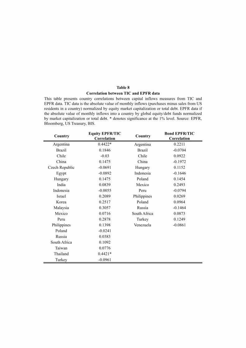
Country Equity EPFR/TIC Correlation Country Bond EPFR/TIC
CorrelationArgentina 0.4422* Argentina 0.2211
Brazil 0.1846 Brazil -0.0704Chile -0.03 Chile 0.0922China 0.1475 China -0.1972
Czech Republic -0.0691 Hungary 0.1152Egypt -0.0892 Indonesia -0.1646
Hungary 0.1475 Poland 0.1454India 0.0839 Mexico 0.2493
Indonesia -0.0055 Peru -0.0794Israel 0.2089 Philippines 0.0269Korea 0.2517 Poland 0.0964
Malaysia 0.3057 Russia -0.1464Mexico 0.0716 South Africa 0.0873
Peru 0.2878 Turkey 0.1249Philippines 0.1398 Venezuela -0.0861
Poland -0.0241Russia 0.0383
South Africa 0.1092Taiwan 0.0776
Thailand 0.4421*Turkey -0.0961
Table 8Correlation between TIC and EPFR data
This table presents country correlations between capital inflows measures from TIC andEPFR data. TIC data is the absolute value of monthly inflows (purchases minus sales from USresidents in a country) normalized by equity market capitalization or total debt. EPFR data ifthe absolute value of monthly inflows into a country by global equity/debt funds normalizedby market capitalization or total debt. * denotes significance at the 1% level. Source: EPFR,Bloomberg, US Treasury, BIS.

Type of estimation
Variable/SampleFull Sample (Didier et al.,
2010)EM+Developed Non-EM
developing Full Sample Full Sample EM+Developed Non-EM developing EM
0.2783*** -0.002 0.4869*** 0.0141*
0.000 0.983 0.001 0.068
0.2149*** 0.072 0.3234*** 0.0113
0.000 0.397 0.018 0.106
0.012* -0.004 0.0382** -0.0190.091 0.617 0.027 0.192
S&P Returns*US Absolute Flows
US Absolute Flows
0.8549*** 0.8549*** 1.080*** 0.7516*** 1.201***0.000 0.000 0.000 0.000 0.000
R-squared 0.558 0.682 0.467 0.347 0.347 0.554 0.274 0.504Observations 1539 651 802 1628 1628 682 858 273
Time dummies Yes Yes Yes No No No No NoCountries 74 31 39 74 74 31 39 21
S&P returns*US Holdings*Post-Lehman
S&P returns*US Holdings
S&P returns
Time dummies, Lehman interaction Replacing time dummies by S&P returns
This table presents stress tests to estimations in Didier et al., 2010. First three columns presents data from Didier et al., and their methodology. Returns are normal local returns, are filtered leavingoutliers out, and US Holdings are normalized by substracting its sample average and dividing it by its sample standard deviation. Additionally their crisis period are defined as 6/2007 to 4/2009 asopposed to the 03/2008-03/2009 crisis period used in this paper. In turn, columns 4-10 are presented for the same data but with our methodology. Returns are dlog(stock_index) and does not filterany local stock market returns. *, **, *** Denote significance at the 1%, 5%, and 10% levels, respectively. In italics appears the correspondent the p-value. Source: Didier et al,. 2010, Bloomberg,US Treasury.
Table 9Financial globalization and financial recoupling around the crisis
S&P returns*US Holdings*Pre-Lehman

Sample Full Sample Turmoil Normal
S&P Returns 0.586*** 0.579*** 0.841***(0.058) (0.119) (0.137)
S&P Returns*FG Flow 4.204*** 4.879*** 0.739(0.412) (0.787) (0.967)
FG Flow 0.021 0.060 0.094***4.204*** (0.054) (0.029)
Observations 1,449 588 861R-Squared 0.457 0.427 0.201Countries 21 21 21
US HY Returns 0.618*** 0.618*** 0.425***(0.0457) (0.0690) (0.147)
US HY Returns*FG Flow 2.638*** 3.455*** -0.153(0.305) (0.559) (1.650)
FG Flow -0.134* -0.376** -0.297**(0.0691) (0.159) (0.122)
Observations 1005 495 510R-Squared 0.402 0.459 0.060Countries 15 15 15
Broad Dollar Index Returns 1.251*** 1.514*** 0.665***(0.113) (0.218) (0.216)
Broad Dollar Index*FG Flow 1.610 4.568* 0.762(1.452) (2.442) (2.724)
FG Flow -0.0209 -0.0875** -0.0432(0.0260) (0.0391) (0.0364)
Observations 1,173 510 663
FX
Table 10FG and financial recoupling: EPFR Flow Data
This table presents estimations of the relationship between financial recoupling and financialglobalization. All results are from panel estimations with country fixed effects. FG Flows areabsolute values of net inflows to a country by global and global emerging mutual fundsnormalized by market capitalization. Dependent variables are dlog returns from EM assets(MSCI country indexes, sovereign spreads, and exchange rate, LCU/USD). Sample goes from2005-09/2010 due to data availability. Normal and turmoil divides the sample between positive(or zero) and negative returns from the global asset respectively. Robust standard errors inparentheses. *, **, and *** denotes significance at the 10, 5 and 1% level respectively. Source:MSCI, GEM World Bank, Bloomberg, US Treasury, EPFR, Barclays Capital, GEM WorldBank, IMF IFS Statistics.
Equity
Bond

Sample Full Sample Turmoil Normal Full Sample Turmoil NormalInstrument Type External External External Internal Internal Internal
S&P Returns 0.255*** 0.047 0.503*** 0.474*** 0.432*** 0.564***(0.089) (0.140) (0.103) (0.090) (0.113) (0.129)
S&P Returns*FG Flow 7.192*** 8.136*** 3.580*** 4.596*** 5.193*** 2.620**(1.020) (1.366) (0.788) (0.636) (0.765) (1.155)
FG Flow 0.031 0.192*** 0.046 0.053*** 0.119*** 0.017(0.026) (0.049) (0.041) (0.016) (0.025) (0.034)
Observations 1,428 567 861 1,428 567 861
US HY Returns 0.464*** 0.234*** 0.620*** 0.448*** 0.400*** 0.499***(0.0430) (0.0446) (0.166) (0.0507) (0.0546) (0.103)
US HY Returns*FG Flow 4.999*** 8.295*** 1.719 3.857*** 4.408*** 1.528(0.956) (1.609) (3.061) (0.783) (0.877) (1.444)
FG Flow -0.470*** -1.309*** -1.120*** -0.350*** -0.456*** -0.585***(0.165) (0.337) (0.378) (0.123) (0.171) (0.107)
Observations 1,005 495 510 1,005 495 510
Broad Dollar Index Returns 1.077*** 1.094*** 0.774*** 1.140*** 1.277*** 0.859***(0.190) (0.243) (0.199) (0.185) (0.219) (0.165)
Broad Dollar Index*FG Flow 5.494 6.055 -0.983 1.100 1.381 -1.758(3.773) (4.760) (3.482) (1.449) (1.957) (1.170)
FG Flow -0.0283 -0.241*** -0.0917** -0.0624** -0.0352 -0.128***(0.0292) (0.0757) (0.0434) (0.0308) (0.0442) (0.0242)
Observations 1,156 493 663 1,156 493 663
Table 11
Equity
Bond
FX
This table presents estimations of the relationship between financial recoupling and financial globalization. All results are from Arellano and Bonddifference estimator. FG Flows are absolute values of net inflows to a country by global and global emerging mutual funds normalized by marketcapitalization. Dependent variables are dlog returns from EM assets (MSCI country indexes, sovereign spreads, and exchange rate, LCU/USD). Samplegoes from 2005-09/2010 due to data availability. Normal and turmoil divides the sample between positive (or zero) and negative returns from the globalasset respectively. Different type of instruments were used. External indicates that instruments for country i were FG flows to EM minus FG flows tocountry i. Internal indicates that the first lag of the dependent variables were used as instruments. Robust standard errors in parentheses. *, **, and ***denotes significance at the 10, 5 and 1% level respectively. Source: MSCI, GEM World Bank, Bloomberg, US Treasury, EPFR, Barclays Capital, GEMWorld Bank, IMF IFS Statistics.
FG and financial recoupling: Robustness tests and causality

Sample Fund Detail Fund Detail Fund Detail Fund Detail Aggregated Aggregated Aggregated
Country Weight (t-1) 0.956*** 0.956*** 0.956*** 0.904*** 0.963*** 0.96338*** 0.963***(0.002) (0.002) (0.002) (0.005) (0.015) (0.015) (0.016)
Country Weight (t-1)*Crisis Dummy -0.002 -0.00039(0.002) (0.008)
Country Returns (t-1) 0.009 -0.010 -0.021 0.061 0.012 0.00971 0.060(0.047) (0.097) (0.099) (0.109) (0.100) (0.150)
Country FE YES YES YES NO YES YES YESTime FE NO NO YES YES NO NO YES
Fund-Country FE NO NO NO YES NO NO NO
Observations 94,020 94,020 94,020 94,020 1,286 1,286 1,286R-squared 0.974 0.974 0.974 0.976 0.995 0.995 0.995
Country Weight
This table presents estimations country weights on lagged country weights and country returns for international mutual funds. All results are from panel estimations withcountry fixed effects. Country returns are from MSCI country indexes. Dummy crisis is a binary variable that takes the value of 1 between March 2008 and March 2009 andzero otherwise. We exclude data when country weight is equal to zero. Fund detail indicates that we use individual mutual fund data, and Aggregated indicates we useaggregated flow data by country. Data is from 2005-November 2010. Robust standard errors in parentheses. *, **, and *** denotes significance at the 10, 5 and 1% levelrespectively. Source: MSCI, GEM World Bank, Bloomberg, US Treasury, EPFR, Barclays Capital, GEM World Bank, IMF IFS Statistics.
Table 12Benchmarking in Mutual Funds

Figure 1Convergence among EM?
This figure presents the relationship between 5-year average GDP growth forecast (2011-2015) and per capita GDP in USD in 2009 for the sample of EM used in this paper. (*) denotes significance at the 10% level. Source: IMF WEO April 2011.
y = -6E-05x + 5,5093 (*)
R! = 0,1534 0
1
2
3
4
5
6
7
8
9
10
0 5000 10000 15000 20000 25000 30000 35000 40000 45000 50000
5-ye
ar a
vera
ge g
row
th fo
reca
st (2
011-
2015
) in
%
GDP per capita in USD (2009)

Figure 2Coupling in the global cycle
This figure presents the median R-squared among emerging and advanced economies from regressions of growth in country i versus PC1growth in these countries (as a proxy from global growth)
15.5%
23.3%
53.7%
69.8%
0%
10%
20%
30%
40%
50%
60%
70%
80%
EM Advanced
Early (1993-2000) Late (2001-Q3 2010)

Figure 3Seemingly growing correlation between G7 and EM’s growth cycle
This figure presents average 5-year correlation between growth in EM countries and G7 growth. First, 5-year rolling correlations betweenindividual countries and G7 were obtained, and then the simple average across emerging countries was taken. Source: IMF WEO April 2011.
-0.8 -0.6 -0.4 -0.2 0.0 0.2 0.4 0.6 0.8 1.0 1.2 1.4 1.6
EM EM+1 SD EM -1 SD

Figure 4Growth outperformance in EM relative to G7
This figure shows EM growth and G7 growth. EM is the simple average of individual countries. Source: IMF WEO April 2011.
-8%
-6%
-4%
-2%
0%
2%
4%
6%
8%
10%
12%
Forecast G7 EM EM +- 1 SD
Forecast

Figure 5Convergence between EM and G7: Alphas and Per capita GDP
This figure presents alphas from estimations in column 4 in Table 3.1 for individual countries and their relationship with initial (1993) GDPper capita PPP. Source: IMF IFS Statistics, IMF WEO
IN
PH
ID PE
TH ZA
PL
TR RU
AR
MX
KR
TW
IL HK
SG
y = -0.015ln(x) + 0.1554 R! = 0.46406
-2%
-1%
0%
1%
2%
3%
4%
5%
6%
7%
8%
0 5000 10000 15000 20000 25000
Alp
ha
Initial (1993) GDP Per Capita PPP

Figure 6Real decoupling in EM: Decoupling with G7 and coupling with China
This figure presents different betas from 2003 to 09/2010. Betas for G7 and China were estimated from dlog(EM) vs dlog(G7) dlog(China), were EM, G7, and China are real gdp growth or industrial production growth in EM countries, the G7 and China respectively. Betas were estimated by extending the time window. The first betaswere estimated with the sample going from 1993 to 2003, and for the rest of the betas we extended the sample until 09/2010. Source: IMF IFS, GEM World Bank.
0.6
0.7
0.8
0.9
1
Real GDP Growth
G7 Beta G7 Beta +- 1 SD Linear (G7 Beta)
0.6
0.7
0.8
0.9
1
Real GDP Growth
China Beta China Beta +- 1 SD Linear (China Beta)
0.65 0.7
0.75 0.8
0.85 0.9
Industrial Production Growth
G7 Beta G7 Beta +- 1 SD Linear (G7 Beta)
0.2 0.25 0.3
0.35 0.4
0.45 0.5
Industrial Production Growth
China Beta China Beta +- 1 SD Linear (China Beta)
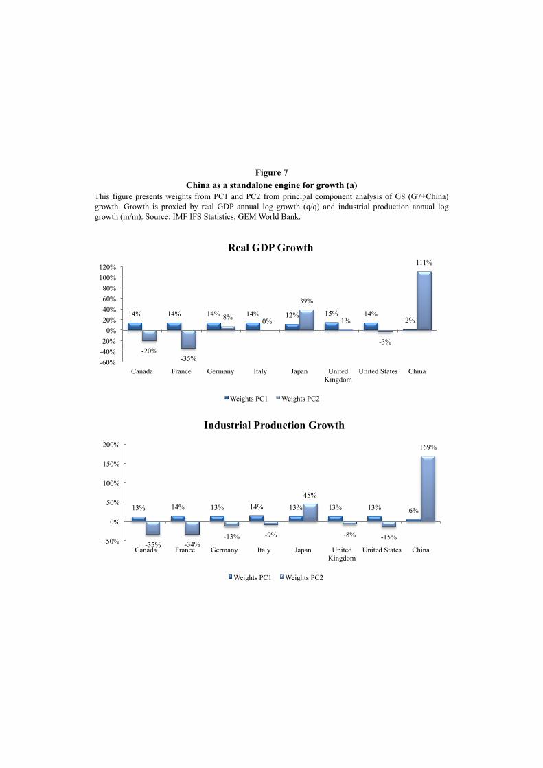
Figure 7China as a standalone engine for growth (a)
This figure presents weights from PC1 and PC2 from principal component analysis of G8 (G7+China)growth. Growth is proxied by real GDP annual log growth (q/q) and industrial production annual loggrowth (m/m). Source: IMF IFS Statistics, GEM World Bank.
14% 14% 14% 14% 12% 15% 14% 2%
-20% -35%
8% 0%
39%
1%
-3%
111%
-60% -40% -20%
0% 20% 40% 60% 80%
100% 120%
Canada France Germany Italy Japan United Kingdom
United States China
Real GDP Growth
Weights PC1 Weights PC2
13% 14% 13% 14% 13% 13% 13% 6%
-35% -34% -13% -9%
45%
-8% -15%
169%
-50%
0%
50%
100%
150%
200%
Canada France Germany Italy Japan United Kingdom
United States China
Industrial Production Growth
Weights PC1 Weights PC2

Figure 8China as a standalone engine for growth (b)
This figure presents R-squared from individual regressions of growth vs PC1 or PC2 from principalcomponent analysis of G8 (G7+China) growth. Growth is proxied by real GDP annual log growth (q/q)and industrial production annual log growth (m/m). Source: IMF IFS Statistics, GEM World Bank.
78% 79% 82% 79%
57%
87% 79%
2% 1% 5% 2% 1%
19%
1% 0%
89%
0%
20%
40%
60%
80%
100%
Canada France Germany Italy Japan United Kingdom
United States China
Real GDP Growth
R-Squared PC1 R-Squared PC2
63%
86% 78%
88% 78% 73% 71%
13% 2% 2% 0% 0%
12% 0% 0%
81%
0%
20%
40%
60%
80%
100%
Canada France Germany Italy Japan United Kingdom
United States China
Industrial Production Growth
R-Squared PC1 R-Squared PC2

Figure 9EM Assets co-movement
This figure presents median R-squared from estimations of individual country's assets log returns (Equity/Spreads/FX) against the PC1 of thelog returns in these EM. Source: Bloomberg, MSCI, GEM World Bank.
36%
52%
25%
62% 67%
37%
68%
78%
47%
0%
10%
20%
30%
40%
50%
60%
70%
80%
90%
Equity Spreads FX
2000-2004 2005-2008M02 2005-2010

Figure 10EM Assets' Betas during the 2000s
This figure presents betas from country-by-country estimations of dlog(EM Asset) vs dlog(Global Asset) during 2000-2004 and 2005-2010. EM assets are MSCI countryindexes, exchange rates and EM sovereign credit spreads. Global assets are the S&P, the Broad Dollar Index and the US HY corporate spread. Source: Bloomberg, MSCI,GEM World Bank, US Treasury.
Chile Israel
Korea Turkey
0
0.5
1
1.5
2
0 0.5 1 1.5 2
Lat
e (2
005-
2010
)
Early (2000-2004) Betas-Equity Linear (45° Line)
Brazil
Chile Turkey
-0.2
0.3
0.8
1.3
-0.2 0 0.2 0.4 0.6 0.8 1 1.2
Lat
e (2
005-
2010
)
Early (2000-2004) Betas-Spreads Linear (45° Line)
Indonesia
Philippines Thailand
-0.5 0
0.5 1
1.5 2
2.5
-0.5 0 0.5 1 1.5 2 2.5
Lat
e (2
005-
2010
)
Early (2000-2004) Betas-FX Linear (45° Line)

Figure 11Financial globalization through global equity funds
This figure presents the percentage of assets invested in Advanced and Emerging markets by global equity funds. Source: EPFR
0%
2%
4%
6%
8%
10%
12%
14%
16%
74%
76%
78%
80%
82%
84%
86%
88%
Advanced EM

Figure 12High alpha, high beta pattern
This figure presents log(EM Asset) and log(Global Asset) during 2005-2010. EM assets are MSCI EM, FX-EM and EMBI Global. FX-EM is an index that averages dlogchanges across EM' FX. Global assets are the S&P, the Broad Dollar Index and the US HY corporate spread. Source: Bloomberg, MSCI, GEM World Bank, US Treasury.
4
4.5
5
5.5
ln(MSCI EM) ln(MSCI World)
3
4
5
6
ln(EMBI Global) ln(US HY)
4.2 4.3 4.4 4.5 4.6 4.7 4.8
ln(FX-EM) ln(Broad Dollar Index)

Figure 13Crisis equity betas (2008-2009) vs US Holdings
This figure presents the scatter plot of betas during the crisis (as country-by-country estimations of local returns vs S&P) against US holdings offoreign equity instruments normalized by equity market capitalization at the end of 2007. ** denotes significance at the 5% level. Source: Didier etal,. 2010, US Treasury, Bloomberg.
y = -1,3322x + 1,4621 R! = 0,1197
y = -0,808x + 1,5113 R! = 0,0434
y = 1,2321x + 1,0055 R! = 0,0139
(**)
-0.5
0.0
0.5
1.0
1.5
2.0
2.5
0% 5% 10% 15% 20% 25% 30% 35% 40%
Bet
as
US Holdings/Mcap
EM + Developed EM Frontier