Emergent self-organizing feature map for recognizing road sign images

ORIGINAL ARTICLE

Emergent self-organizing feature map for recognizingroad sign images

Yok-Yen Nguwi • Siu-Yeung Cho

Received: 28 January 2009 / Accepted: 15 October 2009 / Published online: 3 November 2009

� Springer-Verlag London Limited 2009

Abstract Road sign recognition system remains a chal-

lenging part of designing an Intelligent Driving Support

System. While there exist many approaches to classify road

signs, none have adopted an unsupervised approach. This

paper proposes a way of Self-Organizing feature mapping

for recognizing a road sign. The emergent self-organizing

map (ESOM) is employed for the feature mapping in this

study. It has the capability of visualizing the distance

structures as well as the density structure of high-dimen-

sional data sets, in which the ESOM is suitable to detect

non-trivial cluster structures. This paper discusses the

usage of ESOM for road sign detection and classification.

The benchmarking against some other commonly used

classifiers was performed. The results demonstrate that the

ESOM approach outperforms the others in conducting the

same simulations of the road sign recognition. We further

demonstrate that the result obtained with ESOM is signif-

icantly more superior than traditional SOM which does not

take into the boundary effect like ESOM did.

Keywords Self-organizing map � Data visualization �Image classification � Road sign recognition

1 Introduction

Self-organizing map (SOM), proposed by Kohonen [1, 2],

can be used for dimension reduction, vector quantization,

and visualization. Some recent SOM-based applications in

image processing and pattern recognition domains can be

seen in [3–5]. SOM quantizes input data to a small number

of neurons and still preserves the topology of input data.

Indeed, SOM can be seen as discrete approximation of

principal surfaces in input space [6, 7]. Many visualization

methods based on SOM were proposed, for examples in

[8–11]. Conventional SOM topology seems to be inher-

ently limited by the fixed network. One must adopt a

number of trials and tests to select an appropriate network

structure and size. Several improved SOMs or related

algorithms have been developed to overcome these short-

comings. All these algorithms are mainly in the direction of

growing an SOM adaptively. Although most of these

extended algorithms are able to dynamically increase the

network to an appropriate size, it may not be easy to use the

final SOM maps for visualizing high-dimensional input

data on a 2-D plane, or for distinguishing clusters on a 2-D

plane.

Recently, the ViSOM [12], a new visualization method,

regularizes the inter-neuron distances such that the inter-

neuron distances in the input space resemble those in the

output space after the completion of training. This feature

can be useful to some applications because it is able to

preserve the topology information as well as the inter-

neuron distances. This characteristic is attributed to the

output topology pre-defined in a regular 2-D grid so that

the trained neurons are almost regularly distributed in the

input space. The ViSOM delivers better data visualization

compared with conventional SOM and other visualization

methods.

Another recent approach for SOM-based visualization is

called emergent SOM (ESOM) [13]. Emergent SOM is an

extension of SOM that allows the emergence of intrinsic

structural features of high-dimensional data onto a two-

dimensional map. It has been demonstrated that using

Y.-Y. Nguwi � S.-Y. Cho (&)

Division of Computing Systems, School of Computer

Engineering, Nanyang Technological University,

Nanyang Avenue, Singapore 639798, Singapore

e-mail: [email protected]

123

Neural Comput & Applic (2010) 19:601–615

DOI 10.1007/s00521-009-0315-6

ESOM is a significantly different process from using k-

means. ESOM is a powerful tool for clustering, visualiza-

tion, and classification.

In this paper, we propose the visualization of road sign

images through the methodology of feature clustering and

visualizing by emergent self-organising map (ESOM). The

observation obtained through the visualization process will

be discussed. Six classes of road signs are investigated;

they are namely stop sign, give-way sign, no left turn sign,

no right turn sign, speed limit 60 km/h and speed limit

90 km/h. The focus of this work is to show how the ESOM

can be used as an unsupervised network that is able to

segregate the six classes of the road signs. Due to the lack

of publicly available road sign database, this work

describes and makes available a road sign database that

consist of 447 road scene images and 1,600 road sign

images.

The paper is organized as follows: Sect. 2 describes

some related background works and motivation of pro-

posing a road sign recognition system. Section 3 gives an

overview on the usage of ESOM. Section 4 presents the

visualization and classification performances of using

ESOM on the road sign image. Finally, conclusion of this

paper is drawn in Sect. 5.

2 Related works and motivations

In recent years, the works on developing road sign rec-

ognition system are numbered. However, it is a very

important area that deserves wider attention. A road sign

recognition system provides timely alert to warn the dri-

ver of any critical sign ahead. The objective of a road

sign recognition system is to detect and classify one or

more road signs from coloured images captured by

camera. There exist many challenges that such a system

should address. For instances, lighting condition is a very

difficult problem to regulate. The strength of the light

depends on the time of the day and season, and also on

the weather conditions. In addition, road sign patterns

within images can be affected by shadows from sur-

rounding objects.

In general, a road sign recognition system will first

detect the road sign of interest in the image followed by

classifying it into different classes. Most of the solutions

rely on the colour and shape of the road sign. Colour is a

visual feature that represents the most significant clue that

can be easily noticed by the driver. The colours that are

used in road signs are regulated by different countries and

are often simple primary colours (red, green, or blue) with

the exception of yellow, a secondary colour. Colour-based

detection methods aim to segment the typical colours of

road signs in order to provide a region of interest for further

processing. Some colour-based detection methods are

colour thresholding [14], HSI transformation [43], colour

indexing [40], dynamic pixel aggregation [15], and region

growing [40]. A recent work by Ruta [37] represents the

road sign using discrete colour information with colour

distance transform. The accuracy is about 74.4%.

Shape, being one of the two important attributes of

road signs, can also be used for road sign recognition.

Some shape detection approaches work without the use of

colour information. However, the selection of a scheme

for the detection of road signs based on their shapes will

have to address more issues than their colour. For

example such issues as road signs in cluttered scenes,

imperfect shape, as well as variance in scale and size

make the detection task very challenging. Some imple-

mented shape-based methods are hierarchical spatial fea-

ture matching (HSFM) [16], template matching [20], and

distance transform matching [36]. The other methods that

have been implemented successfully in road sign recog-

nition include genetic algorithm [19], similarity measures

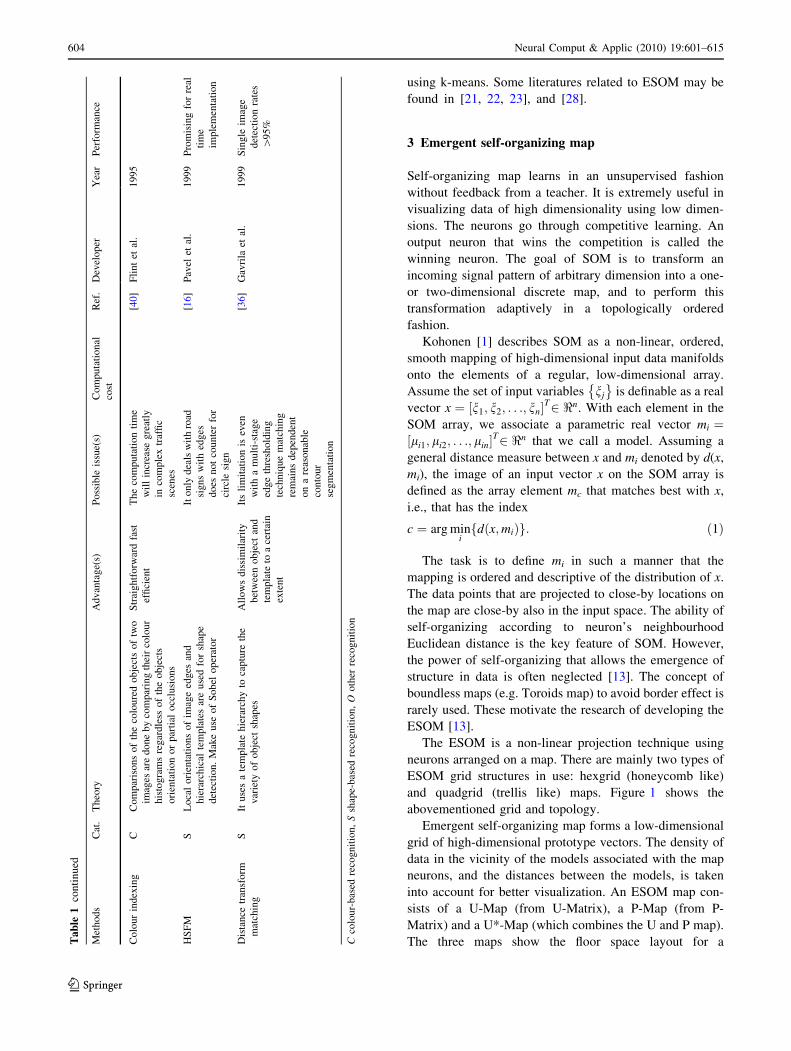
[39], and histographic recognition [32]. Table 1 gives an

overview of the commonly used approaches. The detailed

comparisons of different road sign recognition systems

can be seen in [40, 41].

Among the different methods that try to solve the road

sign recognition problem, we observe very few self-

organizing approaches. There is a recent work by Miguel

and Alastair [38] who attempt to use self-organizing map

for road sign recognition. They group the road signs

according to pictogram of sign and followed by hierar-

chical classification. But the work does not give details

on the specific types of road signs being recognized.

There is much more room to grow in the area of

supervised learning for road sign recognition. The ratio-

nale behind using a self-organizing approach in the road

sign recognition is that in the context of a driving sup-

port system, the recognition method cannot always be

taught in advance with all possible road signs; for

instance, some countries might have their own particular

road signs. We thereby introduce the use of ESOM that

forms clusters of different road signs by itself. It would

be quite useful to detect and identify the new kinds of

road signs by means of interactive training (or active

learning) system. On the other hand, the maps used by

most SOM applications are usually small and face sig-

nificant performance degradation when run on large data

sets. Training a small SOM on a data set is similar to k-

means clustering with k equals to the number of nodes in

the map. Basically, ESOM is an extension of SOM in

which large numbers of neurons are used to allow

topology preservation and to allow data structure to

emerge on the maps [13]. It has been demonstrated that

using ESOM is a significantly different process from

602 Neural Comput & Applic (2010) 19:601–615

123

Ta

ble

1C

om

par

iso

no

fro

adsi

gn

reco

gn

itio

nap

pro

ach

es

Met

ho

ds

Cat

.T

heo

ryA

dv

anta

ge(

s)P

oss

ible

issu

e(s)

Com

pu

tati

on

al

cost

Ref

.D

evel

op

erY

ear

Per

form

ance

Co

lour

dis

tan

ce

tran

sform

CD

efin

ea

dis

tan

cem

etri

cto

be

use

dfo

r

com

par

iso

ns

bet

wee

nim

age

of

ali

ke

sig

n

ob

serv

ed

Can

mo

del

mult

imo

dal

colo

ur

dis

trib

uti

on

s

25

–3

0F

ps

[37

]A

nd

rzej

etal

.2

01

07

94

–9

7.3

%

Fu

zzy

AR

TM

AP

CM

akes

use

of

mult

iple

stag

es.

Fir

st

det

erm

ines

the

bord

erof

the

sign

foll

ow

ed

by

pic

tog

ram

[42

]F

ley

ehet

al.

20

06

96

.7%

on

spee

d

lim

itsi

gn

.9

0%

on

ov

eral

l

Rin

gp

arti

tio

ned

ST

he

imag

eis

div

ided

by

sev

eral

con

cen

tric

area

sli

ke

rig

hts

Th

em

atch

ing

pro

cess

is

do

ne

by

com

pu

tin

gth

eh

isto

gra

m

dis

tan

ces

for

all

rin

gs

of

the

imag

esb

y

intr

od

uci

ng

the

wei

gh

tsfo

rev

en/r

ing

Do

esn

’tre

qu

ire

man

y

sam

ple

so

fsi

gn

imag

es

Pro

ble

mm

ayar

ise

for

seg

men

tati

on

of

traf

fic

sig

n

acco

rdin

gto

cert

ain

colo

ur

and

occ

lud

ed

ob

ject

0.1

4s

[30

]S

oet

edjo

etal

.2006

Mat

chin

gra

te

*9

3.9

%

Nea

rest

nei

ghbour

clas

sifi

cati

on

0A

nim

age

inth

ete

stse

tis

reco

gn

ized

by

assi

gnin

gto

itth

ela

bel

of

the

close

st

po

ints

inth

ele

arn

ing

set

Th

eim

age

inth

e

lear

nin

gse

tth

atbes

tco

rrel

ates

wit

hth

e

test

imag

eis

then

the

resu

lt

Fas

tan

dsi

mp

le\

1s

P4

2.2

GH

z

51

2M

BR

AM

[31

]E

scal

era

etal

.2

00

49

8%

hit

rate

Co

lour

thre

sho

ldin

g

segm

enta

tion

CC

om

par

esth

eco

lou

rp

rop

erti

esto

ase

to

f

val

ues

range

and

dec

ide

whic

hca

tegory

this

pix

elb

elon

gs

to

Sim

ple

22

0m

sP

C4

86

33

MH

z

[14

]E

scal

era

etal

.2

00

3

Co

lour

neu

ral

net

work

CT

rain

neu

rons

tore

cog

niz

eco

lou

rso

nro

ad

sig

n.

Cla

ssifi

esea

chp

ixel

wh

ether

the

pix

elh

asa

colo

ur

of

aro

adsi

gn

or

no

t

Fas

tm

atch

ing

adap

tab

le

Req

uir

ela

rge

set

of

trai

nin

gd

ata

totr

ain

up

ag

oo

dn

etw

ork

s

*0

.2s

Pen

tiu

m4

PC

1G

Hz

[44

]F

ang

etal

.2

00

3[

95

%o

fh

itra

te

Pic

togra

mre

cog

nit

ion

CU

sing

ase

ries

of

sig

nim

ages

wit

hh

and

-

defi

ned

reg

ion

so

fin

tere

stto

form

the

bo

rder

lin

eo

fro

adsi

gn

s.T

hes

eim

ages

are

then

use

dfo

rtr

ainin

gth

en

eura

ln

ets

Ver

yfa

stA

dap

tab

leC

ycl

eti

me

bel

ow

20

0m

s

[34

]V

itab

ile

etal

.2

00

2*

90

%o

fh

itra

te

Sp

ace-

var

ian

tse

nso

r

win

do

w

0B

yp

laci

ng

ase

nso

rw

ind

ow

on

the

road

sig

n

cen

tre,

itis

then

able

tore

cog

niz

ero

ad

sig

ns

Invar

iant

wit

hre

spec

t

tov

iew

ing

and

env

iro

nm

enta

l

con

dit

ion

s

Acc

ura

cyd

egra

des

if

the

road

sig

nce

ntr

e

fou

nd

isn

ot

the

actu

alce

ntr

e

0.2

5–

0.4

s,P

23

3[1

7]

Sh

apo

shnik

ov

etal

.2

00

2[

85

%su

cces

sra

te

Tra

nsf

orm

atio

nb

ased

on

CIE

CA

M9

7

mo

del

CF

irst

con

ver

tsR

GB

spac

eto

CIE

stan

dar

d

XY

Asp

ace.

Th

eli

gh

tnes

s,ch

rom

aan

d

hue

(LC

H)

are

then

obta

ined

usi

ng

CIE

CA

M9

7m

od

el

Ites

tim

ates

colo

urs

ver

ycl

ose

tov

iew

er

Ob

ject

sh

avin

g

sim

ilar

colo

ur

to

road

sig

nco

uld

be

seg

men

ted

asw

ell

[33

]G

aoet

al.

20

02

[9

0%

det

ecti

on

hit

Dy

nam

icp

ixel

Ag

gre

gat

ion

CP

roce

sso

nth

eH

SI

colo

ur

spac

e.It

loca

tes

dy

nam

ic,

op

tim

ized

HS

Isu

b-s

pac

es,

acco

rdin

gto

the

satu

rati

on

and

inte

nsi

tyof

the

pro

cess

edo

utd

oo

rim

ages

Red

uce

hu

ein

stab

ilit

y

inre

alsc

enes

[15

]V

itab

ile

etal

.2

00

1[

84

%o

np

enti

um

35

50

MH

z

un

der

lin

ux

HS

Itr

ansf

orm

atio

nC

Enco

des

colo

ur

info

rmat

ion

by

separ

atin

g

ou

tan

ov

eral

lin

ten

sity

val

ue

fro

mtw

o

val

ues

enco

din

gh

ue

and

satu

rati

on

to

mak

eit

mo

reim

mu

ne

toli

gh

tin

gch

ang

es

Ab

leto

seg

men

t

adv

erse

ly

illu

min

ated

road

sign

pro

per

ly:

ver

y

fast

Hu

eis

no

tsu

ited

for

gre

y-l

evel

axis

[43

]P

acli

ket

al.

20

00

*9

5%

of

hit

rate

Neural Comput & Applic (2010) 19:601–615 603

123

using k-means. Some literatures related to ESOM may be

found in [21, 22, 23], and [28].

3 Emergent self-organizing map

Self-organizing map learns in an unsupervised fashion

without feedback from a teacher. It is extremely useful in

visualizing data of high dimensionality using low dimen-

sions. The neurons go through competitive learning. An

output neuron that wins the competition is called the

winning neuron. The goal of SOM is to transform an

incoming signal pattern of arbitrary dimension into a one-

or two-dimensional discrete map, and to perform this

transformation adaptively in a topologically ordered

fashion.

Kohonen [1] describes SOM as a non-linear, ordered,

smooth mapping of high-dimensional input data manifolds

onto the elements of a regular, low-dimensional array.

Assume the set of input variables nj

� �is definable as a real

vector x ¼ n1; n2; . . .; nn½ �T2 <n. With each element in the

SOM array, we associate a parametric real vector mi ¼li1; li2; . . .; lin½ �T2 <n that we call a model. Assuming a

general distance measure between x and mi denoted by d(x,

mi), the image of an input vector x on the SOM array is

defined as the array element mc that matches best with x,

i.e., that has the index

c ¼ arg mini

d x;mið Þf g: ð1Þ

The task is to define mi in such a manner that the

mapping is ordered and descriptive of the distribution of x.

The data points that are projected to close-by locations on

the map are close-by also in the input space. The ability of

self-organizing according to neuron’s neighbourhood

Euclidean distance is the key feature of SOM. However,

the power of self-organizing that allows the emergence of

structure in data is often neglected [13]. The concept of

boundless maps (e.g. Toroids map) to avoid border effect is

rarely used. These motivate the research of developing the

ESOM [13].

The ESOM is a non-linear projection technique using

neurons arranged on a map. There are mainly two types of

ESOM grid structures in use: hexgrid (honeycomb like)

and quadgrid (trellis like) maps. Figure 1 shows the

abovementioned grid and topology.

Emergent self-organizing map forms a low-dimensional

grid of high-dimensional prototype vectors. The density of

data in the vicinity of the models associated with the map

neurons, and the distances between the models, is taken

into account for better visualization. An ESOM map con-

sists of a U-Map (from U-Matrix), a P-Map (from P-

Matrix) and a U*-Map (which combines the U and P map).

The three maps show the floor space layout for aTa

ble

1co

nti

nu

ed

Met

ho

ds

Cat

.T

heo

ryA

dv

anta

ge(

s)P

oss

ible

issu

e(s)

Com

pu

tati

on

al

cost

Ref

.D

evel

op

erY

ear

Per

form

ance

Co

lour

index

ing

CC

om

par

iso

ns

of

the

colo

ure

do

bje

cts

of

two

imag

esar

ed

on

eb

yco

mp

arin

gth

eir

colo

ur

his

togra

ms

reg

ardle

sso

fth

eo

bje

cts

ori

enta

tion

or

par

tial

occ

lusi

ons

Str

aig

htf

orw

ard

fast

effi

cien

t

Th

eco

mp

uta

tio

nti

me

wil

lin

crea

seg

reat

ly

inco

mp

lex

traf

fic

scen

es

[40

]F

lin

tet

al.

19

95

HS

FM

SL

oca

lo

rien

tati

on

so

fim

age

edg

esan

d

hie

rarc

hic

alte

mp

late

sar

eu

sed

for

shap

e

det

ecti

on.

Mak

euse

of

Sobel

oper

ator

Ito

nly

dea

lsw

ith

road

sign

sw

ith

edg

es

do

esn

ot

cou

nte

rfo

r

circ

lesi

gn

[16

]P

avel

etal

.1

99

9P

rom

isin

gfo

rre

al

tim

e

imp

lem

enta

tio

n

Dis

tance

tran

sform

mat

chin

g

SIt

use

sa

tem

pla

teh

iera

rch

yto

cap

ture

the

var

iety

of

ob

ject

shap

es

All

ow

sd

issi

mil

arit

y

bet

wee

no

bje

ctan

d

tem

pla

teto

ace

rtai

n

exte

nt

Its

lim

itat

ion

isev

en

wit

ha

mu

lti-

stag

e

edg

eth

resh

old

ing

tech

niq

ue

mat

chin

g

rem

ain

sd

epen

den

t

on

are

aso

nab

le

con

tou

r

seg

men

tati

on

[36

]G

avri

laet

al.

19

99

Sin

gle

imag

e

det

ecti

on

rate

s

[9

5%

Cco

lou

r-b

ased

reco

gn

itio

n,

Ssh

ape-

bas

edre

cognit

ion,

Oo

ther

reco

gn

itio

n


123

landscape-like visualization for distance and density

structure of the high-dimensional data space. Structures

emerge on top of the map by the cooperation of many

neurons. These emerging structures are the main concept of

ESOM. It can be used to achieve visualization, clustering,

and classification. The different maps for visualization and

the clustering algorithm are introduced in the following

sub-sections.

3.1 Map visualization

Let m:D ? M be a mapping from a high-dimensional data

space D � <n onto a finite set of positions M ¼n1; . . .; nkf g � <2 arranged on a grid. Each position has its

two-dimensional coordinates and a weight vector

W ¼ w1; . . .;wkf g, which is the image of a Voronoi region

in D: the data set E = {x1,…,xd} with xi [ D is mapped to

a position in M such that a data point xi is mapped to its

best-match bm(xi) = nb [ M with d x;wbð Þ� d x;wj

� �;

8wj 2 W , where d is the distance on the data set. The set of

immediate neighbours of a position ni on the grid is

denoted by N(i).

3.1.1 U-map (distance-based visualization)

The U-height for each neuron ni is the average distance of

ni’s weight vectors to the weight vectors of its immediate

neighbours N(i). The U-height, denoted uh(i), is calculated

as follows:

uhðiÞ ¼ 1

n

X

j

d wi;wj

� �; j 2 NðiÞ; n ¼ jNðiÞj: ð2Þ

A display of all U-heights on top of the map is called a

U-Matrix [21]. The height value will be large in area where

no or few data points reside, creating mountain ranges for

cluster boundaries.

3.1.2 P-map (density-based visualization)

The P-height ph(i) for a neuron ni is a measure of the

density of data points in the vicinity of wi:

phðiÞ ¼ j x 2 Ejd x;wj

� �\r

� �; r [ 0; r 2 <j: ð3Þ

A display of all P-heights on top of the grid G is called a

P-matrix [22]. Whereas distance-based methods usually

work well for clearly separated clusters, problems can

occur with slowly changing densities and overlapping

clusters.

3.1.3 U*-map (distance and density based visualization)

The U*-matrix combines the distance-based U-matrix and

the density-based P-matrix. The U*-matrix shows signifi-

cant improvement over U-matrix in dataset with clusters

that are not clearly separated in the high-dimensional

space.

Let uh(i) be denoted by the U-height of a neuron i, ph

denote the mean of all P-heights and maxi

phðiÞf g be the

maximum of all P-heights. The U*-height, denoted as

u*h(i), of an U-Matrix for neuron i is calculated as:

u�h ið Þ ¼ uh ið Þ � k ið Þ; ð4Þ

where k(i) is denoted as a scaling factor which is calculated

as:

k ið Þ ¼ ph ið Þ � ph

ph�maxi

ph ið Þf gþ 1: ð5Þ

With this equation, the scaling factor basically is a linear

function of the P-heights. Using this scaling factor, the U*-

height is equalled to U-height if ph ið Þ ¼ ph of neuron i. We

expect that the probability density function of P-height is

bimodal and its density distribution is a combination of the

within-cluster density distribution and the densities of

weight vectors in between clusters.

3.2 ESOM clustering algorithm

The clustering of ESOM is based on the U*C clustering

algorithm described by [29]. Consider a data point x at

the surface of a cluster C, with a best match of

ni = bm(x). The weight vectors of its neighbours N(i) are

either within the cluster, in a different cluster or inter-

polate between clusters. Assume that the inter-cluster

distances are locally larger than the local within-cluster

distances, then the U-heights in N(i) will be large in such

directions which point away from the cluster C. Thus, a

so-called immersive movement will perform to lead away

from cluster borders.

This immersive movement is performed which starts

from a grid position, keeps decreasing the U-matrix value

Fig. 1 Structures of quad and

hex grid, and topologies of

bounded and boundless

(adapted from [13])


123

by moving to the neighbour with the smallest value, then

keeps increasing the P-matrix value by moving to the

neighbour with the largest value. The details of this clus-

tering algorithm can be referred to Ultsch [29], and the

algorithm is summarized as follows.

Algorithm 1: ESOM Clustering

Given U-Matrix, P-Matrix, U*-Matrix, I = {}.

Immersion

For all positions n of the grid

1. From position n follow a descending movement on the U-Matrix

until the lowest distance value is reached in position u

2. From position u follow an ascending movement on the P-Matrix

until the highest density value is reached in position p

I ¼ I [ pf g; Immersion nð Þ ¼ p

Cluster assignment

1. Calculate the watersheds for the U*-Matrix using the algorithm in

[24]

2. Partition I using these watersheds into clusters C1…Cc

3. Assign a data point x to a cluster Cj if Immersion bm xð Þð Þ 2 Cj

4 Visualization and classification results in road sign

images

This section evaluates the visualization and classification

performance of the ESOM model in the proposed road

sign image recognition task. The creation of database and

the methodology of the road sign image detection are also

described in this section. The overall framework is illus-

trated in Fig. 2. In this framework, regions with potential

road signs are detected by a neural network-based road

sign detection module. Then, the regions of the image

containing potential road sign patterns are extracted, and

the extracted features are used as input to the ESOM. The

detection module segments the input image and extracts

out the areas that contain road sign patterns. We adopted

the holistic approach that searches the whole image for

possible road signs to ensure no road sign is missed out.

The map of the extracted observations is then created and

further analysed to identify the type of road signs they

represented. We have collected 447 different road scene

images in which six categories of road signs with totally

480 images were selected for the experiment in this work.

They are stop, give-way, no left turn, no right turn, speed

limit 60 and speed limit 90 signs as shown in Fig. 3.

These categories were chosen based on an observation

made by the authors and due to higher chances of

occurrence on the road. We first introduce the dataset we

collected; next we go into different parts of the system to

explain the details.

4.1 Road sign database

To the best of our knowledge, little efforts were observed

trying to a publicize road sign database. It has yet to be

known any common road sign database that enables the

benchmarking of road sign recognition systems. The dat-

abases used by researchers in this field are generally small

and lack standardization. This is evident from the work of

Soetedjo and Yamada [30] with 180 images, Escalera [31]

who used 50 images, and Gao [33] who used only 41

images. The problem with working with such small data-

sets is that it is difficult to evaluate the reliability of the

results. There are some with large databases like Vitabile

[34] with 620 images, Paclik [35] with 1,200 images and

Gavrila [36] with 1,000 images. The main concern is that

those databases are not publicly available. Collecting the

road signs images is very time consuming due to the fact

that there are so many different types of road signs avail-

able. And each type of road signs must be sufficiently

collected in order for the experiments to be fruitful. Road

signs vary from country to country; the categories of road

sign also differ. All these make the construction of a

standardized road sign database a real challenge.

We thereby made our road sign database publicly

available together with this work. There are a total of 447

road scene images that contain road signs and about 1,600

cropped road signs. We started with observing the road

signs along the expressway and summarized the number of

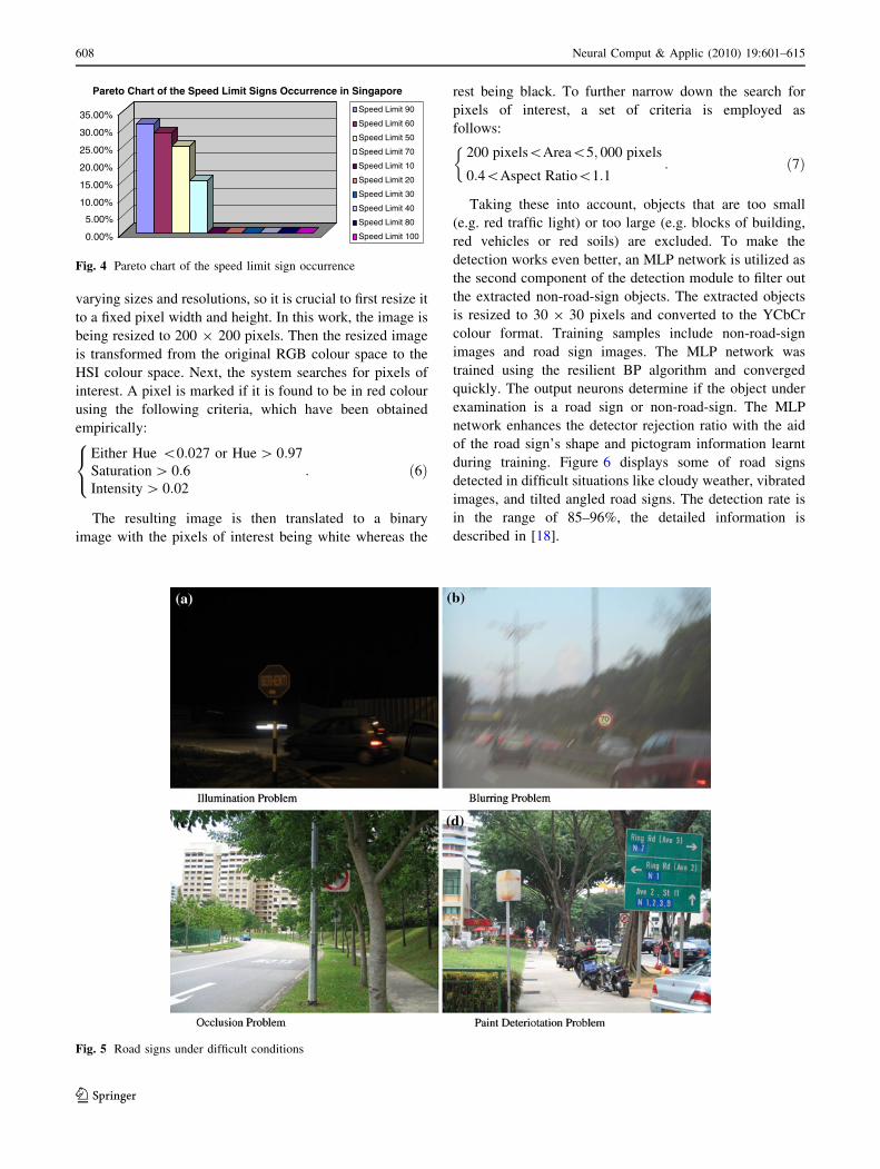
speed limit signs occurrence into Table 2 and Fig. 4, which

comprises of 80 observations. Based on the number of

occurrence of the speed limit signs, the top two frequently

seen speed limit signs are chosen. From the survey, some

speed limit signs are hardly captured like speed limit 10,

20, 30, 40, 80, and 100 km/h. Based on the survey, speed

limit 60 km/h and speed limit 90 km/h are more frequently

seen when compared to others, and hence they are chosen

for implementation in this work together with stop, give-

way, no left turn, and no right turn signs. However, the

database itself contains road signs like give-way sign, no

entry, no left turn, no right turn, speed limit 10 km/h till

speed limit 100 km/h, regulatory and warning signs. On top

of that, some commonly confused objects on the road are

included in the databases which are useful for training

neural network-based road sign recognition system to

reject non-road-sign images. The road scene images com-

prises difficult road scene situations like road sign changes

in position, scale, rotation, illumination problem caused by

different weather condition (Fig. 5a), image blurring

(Fig. 5b), partial occlusion (Fig. 5c), degradation of the

sign colours (Fig. 5d), and the similar objects as road signs.

We have chosen some standardized road signs like stop

signs, no left turn, no right turn, give-way, no entry, and


123

speed limit signs. The cropped road signs are standardized

road signs that are regulated by many countries like United

Kingdom, United States, and European countries.

4.2 Road sign acquisition and extraction

The main task of the road sign acquisition and extraction is

to segment the input image and extract out the areas that

contain road sign patterns. It consists of two components:

segmentation and filtering. In our work, we adopted the

hue-saturation-intensity (HSI) transformation as it is

appealing in colour segmentation because it gives unique

information for different colour component. The HSI seg-

mentation performs the segmentation according to the

nature of the raw images. The raw image could be in

Fig. 2 The overall framework for road sign image processing

Fig. 3 Six selected road signs

for classification. a stop sign, bgive-way sign, c no left turn

sign, d no right turn, e speed

limit 60 km/h sign, and f speed

limit 90 km/h sign

Table 2 Speed limit signs occurrence in Singapore

Speed limit sign (km/h) No. of occurrence Percentage

Speed limit 10 0 0.00










Total 80 100.00


123

varying sizes and resolutions, so it is crucial to first resize it

to a fixed pixel width and height. In this work, the image is

being resized to 200 9 200 pixels. Then the resized image

is transformed from the original RGB colour space to the

HSI colour space. Next, the system searches for pixels of

interest. A pixel is marked if it is found to be in red colour

using the following criteria, which have been obtained

empirically:

Either Hue \0:027 or Hue [ 0:97

Saturation [ 0:6Intensity [ 0:02

8<

:: ð6Þ

The resulting image is then translated to a binary

image with the pixels of interest being white whereas the

rest being black. To further narrow down the search for

pixels of interest, a set of criteria is employed as

follows:

200 pixels\Area\5; 000 pixels

0:4\Aspect Ratio\1:1

�: ð7Þ

Taking these into account, objects that are too small

(e.g. red traffic light) or too large (e.g. blocks of building,

red vehicles or red soils) are excluded. To make the

detection works even better, an MLP network is utilized as

the second component of the detection module to filter out

the extracted non-road-sign objects. The extracted objects

is resized to 30 9 30 pixels and converted to the YCbCr

colour format. Training samples include non-road-sign

images and road sign images. The MLP network was

trained using the resilient BP algorithm and converged

quickly. The output neurons determine if the object under

examination is a road sign or non-road-sign. The MLP

network enhances the detector rejection ratio with the aid

of the road sign’s shape and pictogram information learnt

during training. Figure 6 displays some of road signs

detected in difficult situations like cloudy weather, vibrated

images, and tilted angled road signs. The detection rate is

in the range of 85–96%, the detailed information is

described in [18].

0.00%

5.00%

10.00%

15.00%

20.00%

25.00%

30.00%

35.00%

Pareto Chart of the Speed Limit Signs Occurrence in Singapore

Speed Limit 90

Speed Limit 60

Speed Limit 50

Speed Limit 70

Speed Limit 10

Speed Limit 20

Speed Limit 30

Speed Limit 40

Speed Limit 80

Speed Limit 100

Fig. 4 Pareto chart of the speed limit sign occurrence

Fig. 5 Road signs under difficult conditions


123

4.3 Road sign feature extraction and representation

Meaningful information is hidden underneath the road sign

image. Proper selection of features optimizes the perfor-

mance of classification. Feature extraction forms the basic

building block of the recognition problem. In this study, we

used the Gabor filtering technique to extract the dominant

features of different road signs. In fact, Gabor wavelet is a

popular choice because of its capability to approximate

mammals’ visual cortex. The primary cortex of human

brain interprets visual signals. It consists of neurons, which

respond differently to different stimuli attributes. The

receptive field of cortical cell consists of a central ON

region surrounded by 2 OFF regions, each region elongated

along a preferred orientation [25]. According to Jones and

Palmer, these receptive fields can be reproduced fairly well

using Daugman’s Gabor function [26]. There is consider-

able evidence that the parameterized family of 2-D Gabor

filters, proposed by Daugman in 1980, suitably models the

profile of receptive cells in the primary visual cortex.

Gabor filters model the properties of spatial localization,

orientation selectivity, and spatial frequency selectivity and

phase relationship of the receptive cells. The Gabor

wavelet function can be represented by:

gðx; yÞ ¼ g1ðx; yÞ expðj2pWxÞ ð8Þ

where

g1ðx; yÞ ¼1

2prxry

� �exp �1

2

x2

r2x

þ y2

r2y

! !

: ð9Þ

We consider that the receptive field (RF) of each cortical

cell consists of a central ON region (a region excited by

light) surrounded by two lateral OFF regions (excited by

darkness) [27]. Spatial frequency (W) determines the width

of the ON and OFF regions. rx2 and ry

2 are spatial variances

which establish the dimension of the RF in the preferred

and non-preferred orientations.

An image is convolved with all these filters so as to

extract the image features. The lower bound frequency is

chosen as 0.05, while the upper bound frequency is chosen

to be 0.4. Orientations are in multiples of p6

from 0 to p.

After the Gabor feature extraction process, a number of

Gabor filtered images are generated. This appears to be a

huge dataset to be realized, and the images may include

redundant information. Therefore, feature selection is

essential. In the feature selection step, the Gabor images

generated for a road sign are transformed into a single

image that theoretically has the same dimension as the

Fig. 6 Images used in

evaluating detection module


123

original image, but the dataset undergoes dimensionality

reduction. In this work, principle component analysis

(PCA) is used to shrink down the dimensions. PCA is a

useful technique that has been widely used in vast appli-

cations for reducing dimensionality, visualization, and

finding patterns or clusters in high-dimensional data. The

similarities and differences of data can be shown through

the use of PCA. Figure 7 shows the responses of the dif-

ferent road sign images by processing with Gabor filtering

and further processing with PCA. The filter bank consists

of 24 different filters with 6 different orientations (from 0

to p) and 4 different scales. Image features were repre-

sented using the full convolution results of the image with

different Gabor kernels. Each road sign image was filtered

with one filter, thus the filtered output would be of size

30 9 30 (i.e. a 900-dimensional vector). So, 24 sets of

filtered vectors were concatenated horizontally to form an

input matrix of size 900 9 24 for PCA operation. We then

extracted the first PCA component corresponding to the

highest eigenvalue to produce a 900 9 1 input vector to be

learnt and classified by SOM at the later stage.

4.4 Road sign features visualization

This section presents the visualization results for

representing road sign feature in ESOM feature map. The

whole data set (i.e. 447 road sign images) was trained with

map size 20 9 20. For the purpose of validation, a number

of Gabor filters were generated in the range from one

Gabor up to 24 Gabors, and the resulting road sign features

would be used for visualization and classification by the

SOM feature map. The visualization results by both SOM

and ESOM feature mapping are shown in Figs. 8 and 9

respectively. All the maps shown in Fig. 8 are the general

U-matrix obtained by the SOM visualization, whereas all

the maps shown in Fig. 9 are both U-matrix and P-matrix

obtained by the ESOM visualization. The six road signs are

labelled as different colours. The little circle shown inside

each neuron represented the test output that maps to the

corresponding neuron in the SOM maps. The colour of the

little circle denotes the class of the test point. We have

adopted 2-D toroid structure with Euclidean distance for

ESOM. The ESOM output is then shown to have connected

boundary effect, as shown in both U-matrix and P-matrix,

for example the give-way sign in yellow from Fig. 9 and

the no right turn in pink that is distributed around the edges

of the map. The ESOM provides a low-dimensional pro-

jection preserving the topology of the input space, thus the

high-dimensional distances can be visualized with the

canonical U-Matrix, P-Matrix and U*-Matrix together so

that the cluster boundaries can be distinguished more

sharply. In addition, the visualization by the ESOM feature

map can be interpreted as height values on top of the

usually two-dimensional grid of the SOM, leading to an

intuitive paradigm of a landscape. Based on looking at the

results, it seems that using the ESOM feature map with 4

Gabor filtering has the best visualization quality of map-

ping effects among the maps with other number of Gabor

filters. Most of the road signs included give way, no left

turn, no right turn, speed limit 60 and speed limit 90 which

are able to form closed regions on the map, whereas there

is one road sign, i.e., stop that formed more than one region

in the map. In particular, the stop sign is often mapped in

different and separate regions. It is because the stop sign

may contain outliers within both areas of the give-way sign

and speed limit 90. It is similar to the mapping of the No

right turn with one Gabor filter used, which contains some

outliers within both areas of the speed limit 60 and speed

limit 90 signs. The mapping of the no left turn sign with 24

Gabors used is even worse as it became outliers and noises

by the other road signs so it populated to different regions.

This probably ‘‘confused’’ by the combination of Gabor

and PCA feature extraction in which the extracted features

of no left turn are quite similar to the other road signs, like

no right turn or speed limit sign, creates a rather random

mapping. In summary, most of the road signs can be

mapped by the ESOM, and the visualization results

obtained by the ESOM can help in recognizing and clas-

sifying consistent road signs in unlabelled datasets.Fig. 7 Intermediate images of 6 classes of road signs. a Stop, b give-

way, c no left turn, d no right turn, e speed limit 60, and f speed limit 90


123

4.5 Road sign classification

For classification of task, labelling all (or most) neurons

instead of only the best matches created a classification

method based on unsupervised training which is similar to

a k-nearest neighbour (kNN) classifier with k = 1 that can

be applied to new data automatically. The main difference

to kNN is that the user can use the visualization of the

ESOM to create the labelling, whereas kNN does not give

any visualization that could be used for this purpose. Fur-

ther, kNN classification always classifies a point, no matter

how near (or far) the neighbours are. In contrast, ESOM

classification offers an unknown class by leaving neurons

unlabelled, for example, for sparsely populated regions

separating clusters.

This section presents to use ESOM classification to

classify the road sign images. Ten-folds cross validation

has been conducted. Each fold contains eight images for

each class. We first compare the results obtained from

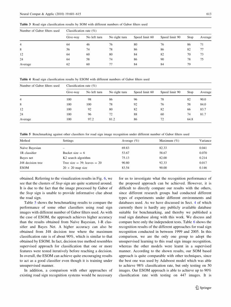
SOM and ESOM classifiers. Tables 3 and 4 summarize the

classification results of ten-folds cross validation obtained

from the SOM and ESOM, respectively. There are four sets

of results involved in the feature map. The first set uses

four Gabor wavelets and takes PCA of the convoluted

images, and it produces average hit rate of 90.0% for

ESOM which is much higher than 71% achieved from

traditional SOM. The second set extracts from PCA image

of eight wavelets, and its hit rate is about 84.0% for ESOM

and 77% for SOM. The third set uses twelve Gabor

wavelets; the hit rate is about 83.7% for ESOM, almost

Fig. 8 The Self-Organizing

Feature Maps for Road Sign

Images. a 1 Gabor used, b 4

Gabors used, c 8 Gabors used, d12 Gabors used, e 24 Gabors

used, f the color legend


123

10% higher than SOM. The last set takes 24 Gabor

wavelets and gives the hit rate as 81.7%. It is observed that

the best hit-rate of 90% could be obtained by using 4 Gabor

wavelets for feature extraction. Looking into individual

road signs, the five classes of road signs are quite compa-

rable excluding Stop sign in which about 65% hit-rate was

Fig. 9 The Emergent Self-Organizing Feature Maps (U-matrix and

P-matrix) for Road Sign Images. a 1 Gabor used in U-matrix, b 1

Gabor used in P-matrix, c 4 Gabors used in U-matrix, d 4 Gabors used

in U-matrix, e 8 Gabors used in U-matrix, f 8 Gabors used in P-

matrix, (g) 12 Gabors used in U-matrix, (h) 12 Gabors used in P-

matrix (i) 24 Gabors used in U-matrix, (j) 24 Gabors used in P-matrix

(k) the colour legend


123

obtained. Referring to the visualization results in Fig. 6, we

see that the clusters of Stop sign are quite scattered around.

It is due to the fact that the image processed by Gabor of

the Stop sign is unable to provide informative clue about

the road sign.

Table 5 shows the benchmarking results to compare the

performance of some other classifiers using road sign

images with different number of Gabor filters used. As with

the case of ESOM, the approach achieves higher accuracy

than the results obtained from Naıve Bayesian, 1-R clas-

sifier and Bayes Net. A higher accuracy can also be

obtained from J48 decision tree where the maximum

classification rate is of about 90%, which is similar to that

obtained by ESOM. In fact, decision tree method resembles

supervised approach for classification that one or more

features were tested iteratively before reaching a decision.

In overall, the ESOM can achieve quite encouraging results

to act as a good classifier even though it is training under

unsupervised manner.

In addition, a comparison with other approaches of

existing road sign recognition systems would be necessary

for us to investigate what the recognition performance of

the proposed approach can be achieved. However, it is

difficult to directly compare our results with the others,

since different research groups had conducted different

types of experiments under different environments and

databases used. As we have discussed in Sect. 4 of which

currently there is hardly any publicly available database

suitable for benchmarking, and thereby we published a

road sign database along with this work. We discuss and

compare here only the independent tests. Table 6 shows the

recognition results of the different approaches for road sign

recognition conducted in between 1999 and 2005. In this

comparison, we are the only one group to adopt the

unsupervised learning to this road sign image recognition,

whereas the other models were learnt in a supervised

manner. According to the shown results, our SOM based

approach is quite comparable with other techniques, since

the best one was used by Adaboost model which was able

to achieve 98% classification rate, but only testing on 50

images. Our ESOM approach is able to achieve up to 90%

classification rate with testing on 447 images. It is

Table 3 Road sign classification results by SOM with different numbers of Gabor filters used

Number of Gabor filters used Classification rate (%)

Give-way No left turn No right turn Speed limit 60 Speed limit 90 Stop Average

4 64 46 76 80 76 86 71

8 56 74 78 86 86 82 77

12 64 60 80 84 82 70 73

24 64 58 74 86 90 78 75

Average 62 60 77 84 84 79

Table 4 Road sign classification results by ESOM with different numbers of Gabor filters used

Number of Gabor filters used Classification rate (%)

Give-way No left turn No right turn Speed limit 60 Speed limit 90 Stop Average

4 100 98 86 96 78 82 90.0

8 100 100 78 92 76 58 84.0

12 100 92 80 82 82 66 83.7

24 100 96 72 88 60 74 81.7

Average 100 97.2 81.2 86 72 64.8

Table 5 Benchmarking against other classifiers for road sign image recognition under different number of Gabor filters used

Method Settings Average (%) Maximum (%) Variance

Naıve Bayesian – 69.83 82.33 0.041

1R classifier Bucket size = 6 53.67 58.67 0.070

Bayes net K2 search algorithm 75.13 82.00 0.214

J48 decision tree Tree size = 39; leaves = 20 90.80 92.33 0.017

ESOM 20 9 20 map size 83.54 90.00 0.146


123

demonstrated that our result is quite encouraging and

comparable.

5 Conclusion

This paper described a novel methodology of recognizing

road sign images using ESOM. ESOM is a powerful tool

for clustering and classification. It is quite useful for

analysing the road sign images under different scenarios.

Unlike the conventional SOM and/or other classifiers that

rely on labelling all or most neurons in the topological

map to perform the classification task, the ESOM

approach does not require to be labelled in a priori which

can help detect classes not seen in training. The capability

of visualization of ESOM enables us to analyse the high-

dimensional space of image features in an intuitive way,

although a large amount of neurons may be required, and

hence the computation may be heavy. Based on the

experimental results, it is demonstrated that the road sign

recognition by ESOM gives better classification than that

by SOM.

References

1. Kohonen T (1990) Self-organizing map. Proc IEEE 78(9):1464–

1480

2. Kohonen T (2001) Self-organizing maps, 3rd edn. Springer,

Berlin

3. Chang C-H, Xu P, Xiao R, Srikanthan T (2005) New adaptive

color quantization method based on self-organizing maps. IEEE

Trans Neural Networks 16(1):237–249

4. Hu W, Xie D, Tan T (2004) A hierarchical self-organizing

approach for learning the patterns of motion trajectories. IEEE

Trans Neural Networks 15(1):135–144

5. Wu S, Rahman MKM, Chow TWS (2005) Content-based image

retrieval using growing hierarchical self-organizing quadtree

map. Pattern Recogn 38(5):707–722

6. Ritter H, Martinetz T, Schulten K (1992) Neural computation and

self-organizing maps: an introduction. Addison-Wesley, Reading

7. Mulier F, Cherkassky V (1995) Self-organization as an iterative

kernel smoothing process. Neural Comput 7:1165–1177

8. Ultsch A, Siemon HP (1990) Kohonen’s self organizing feature

maps for exploratory data analysis. In: Proceedings of the Inter-

national Joint Conf Neural Networks, Paris, France, pp 305–308

9. Pal NR, Eluri VK (1998) Two efficient connectionist schemes for

structure preserving dimensionality reduction. IEEE Trans Neural

Networks 9(6):1142–1154

10. Kong A (2000) Interactive visualization and analysis of hierar-

chical neural projections for data mining. IEEE Trans Neural

Networks 11(3):615–624

11. Wu S, Chow TWS (2005) PRSOM: a new visualization method

by hybridizing multidimensional scaling and self-organizing

map. IEEE Trans Neural Networks 16(6):1362–1380

12. Yin H (2002) ViSOM: a novel method for multivariate data

projection and structure visualization. IEEE Trans Neural Net-

works 13(1):237–243

13. Ultsch A, Morchen F (2005) ESOM-Maps: tools for clustering,

visualization, and classification with Emergent SOM’’, TechnicalReport No. 46, Department of Mathematics and Computer Sci-

ence, University of Marburg, Germany

14. de la Escalera A, Armingol JM, Mata M (2003) Traffic sign

recognition and analysis for intelligent vehicles. Image Vision

Comput 21:247–258

15. Vitabile S, Pollaccia G, Pilato G, Sorbello F (2001) Road signs

recognition using a dynamic pixel aggregation technique in the

HSV color space. In: Proceedings of the 11th international con-

ference on image analysis and processing, Palermo, Italy,

pp 572–577

16. Paclik P, Novovicova J (2000) Road sign classification without

colour information. In: Proceedings of 6th conference of

advanced school of imaging and computing, ASCI, Lommel,

Belgium

17. Shaposhnikov D, Podladchikova LN, Golovan AV, Shevtsova N,

Kunbin AH, Xiaohong G (2002) Road sign recognition by single

positioning of space-variant sensor window. In Proceedings of

15th international conference on vision interface, Canada, Cal-

gary, pp 213–217

18. Nguwi Y, Kouzani AZ (2008) Detection and classification of road

signs in natural environments. Neural Comput Appl 17(3):265–

289

19. Aoyagi Y, Asakura T (1996) A study on traffic sign recognition

in scene image using genetic algorithms and neural networks. In:

Proceedings of the 22nd international conference on industrial

electronics, control, and instrumentation, Taipeis, pp 1838–1843

20. Torresen J, Bakke J, Sekanina L (2004) Efficient recognition of

speed limit signs. In: Proceedings of the 7th international IEEE

conference on intelligent transportation systems, pp 652–656

Table 6 Comparison with other recognition approaches

Approaches Techniques used Database nature Performance

Soetedjio and Yamada (2005) [30] Ring partitioned 180 test images, circular road signs

(no entry, speed limit signs only)

93.9%

Escalera and Radeva (2004) [31] Adaboost and model matching 21 classes, 50 test images 98% on 50 test images

Torresen et al. 2004 [32] Template matching 7 classes of speed limit signs, 198 images 90.9%

Gao et al. (2002) [33] Behavioural model of vision 41 British road sign images 88–90%

Vitabile et al. (2002) [34] MLP neural networks 620 images of 24 classes circular signs -90% of hit rate

Paclik et al. (2000) [35] Laplace Kernel classifier 1,200 images of 50 classes -95% of hit rate

Gavrila and Philomin (1999) [36] Distance transform matching 1,000 traffic sign images -95%

Our approach ESOM based with Gabor features 480 images, 6 classes running under

ten-folds cross validation

78.3–90%


123

21. Ultsch A, Siemon H. (1990). Kohonen’s self organizing maps for

exploratory data analysis. In: Proceedings of international neural

network conference (INNC’90), pp 305–308

22. Ultsch A (2003) Maps for the visualization of high-dimensional

data spaces. In: Proceedings of the workshop on self organizing

maps, Kyushu, Japan

23. Ultsch A (2003) Pareto density estimation: a density estimation

for knowledge Discovery. In: Baier D, Wernecke KD (eds)

Innovations in classification, data science, and information sys-

tems—proceedings 27th annual conference of the german clas-

sification society (GfKL) 2003, Springer, Berlin, Heidelberg,

pp 91–100

24. Luc V, Soille P (1991) Watersheds in digital space: an efficient

algorithm based on immersion simulations. IEEE Trans Pattern

Anal Mach Intell 13(6):583–598

25. La Cara GE, Ursino M (2004) A neural network model of con-

tours extraction based on orientation selectivity in the primary

visual cortex: applications on real images. In: Proceedings of 26th

Annual International Conference of the IEEE EMBS

26. Jones JP, Palmer LA (1987) An evaluation of the two-dimen-

sional gabor filter model of simple receptive fields in cat striate

cortex. J Neurophysiol 58(6):1233–1258

27. La Cara GE, Ursino M, Bettini M (2003) Extraction of salient

contours in primary visual cortex: a neural network model based

on physiological knowledge. Proceedings of the 25th Annual

International Conference of the IEEE 3:2242–2245

28. Ultsch A (2003) U*-Matrix: a tool to visualize clusters in high

dimensional data. Department of Computer Science University of

Marburg, research report 36

29. Ultsch A (2005) Clustering with SOM: U*C, WSOM 2005, Paris,

pp 75–82

30. Soetedjo A, Yamada K (2005) Traffic sign classification using

ring partitioned method. IEICE Trans Fundamentals E88A(9):

166–178

31. de la Escalera A, Radeva P (2004) Fast greyscale road sign model

matching and recognition. In: Vitria J (ed) Recent advances in

artificial intelligence research and development. IOS Press,

Amsterdam, pp 69–76

32. Estevez L, Kehtarnavaz N (1996) A real-time histographic

approach to road sign recognition. In: Proceedings of the IEEE

southwest symposium on image analysis and interpretation,

pp 95–100

33. Gao X, Shevtsova N, Hong K, Batty S, Podladchikova L, Golo-

van A, Shaposhnikov D, Gusakova V (2002) Vision models based

identification of traffic signs. In: Proceedings of the 1st European

conference on color in graphics, image and vision, France,

pp 47–51

34. Vitabile S, Gentile A, Sorbello F (2002) A neural network based

automatic road signs recognizer. Proc 2002 Int Joint Conf Neural

Networks 3:2315–2320

35. Paclik P, Novovicova J, Pudil P, Somol P (2000) Road sign

classification using the Laplace kernel classifier. Pattern Recogn

Lett 21(13–14):1165–1173

36. Gavrila DM, Philomin V. (1999) Real-time object detection for

smart vehicles. In: Proceedings of IEEE international conference

on computer vision, Greece, pp 87–93

37. Ruta A, Li Y, Liu X (2010) Real-time traffic sign recognition

from video by class-specific discriminative features. Pattern Re-

cogn 43(1):416–430

38. Miguel S, Prieto MS, Allen AR (2009) Using self-organising

maps in the detection and recognition of road signs. Image Vis

Comput 27(6, 4):673–683

39. Paclik P, Novovicova J, Duin R (2006) Building road-sign clas-

sifiers using a trainable similarity measure. IEEE Trans Intell

Transp Syst 7(3):309–321

40. Lalonde M, Li Y (1995) Road sign recognition, survey of the

state of the art, Technical report, Centre de Recherche Informa-

tique de Montreal CRIM/IIT

41. Johansson B (2002) Road sign recognition from a moving vehi-

cle, Master’s thesis, Centre for Image Analysis, Uppsala

University

42. Fleyeh H, Gilani S, Dougherty M (2006) Road sign detection and

recognition using Fuzzy ARTMAP: a case study swedish speed-

limit signs. In: Proceedings of Artificial Intelligence and Soft

Computing

43. Paclik P, Novovicova J, Pudil P, Somol P (2000) Road sign

classification using the Laplace kernel classifier. Pattern Recogn

Lett 21(13–14):1165–1173

44. Fang CY, Chen SW, Fuh CS (2003) Road-sign detection and

tracking. IEEE Trans Vehicular Technol 52:1329–1341


123

Documents

Emergent self-organizing feature map for recognizing road sign images