EMERGE Guide Introduction to EMERGE ............................................................................................................... 1 Part 1: Estimating P-wave Velocity from Seismic Attributes....................................................... 2

Starting EMERGE....................................................................................................................... 4 Performing Single-Attribute Analysis....................................................................................... 23 Performing Multi-Attribute Analysis........................................................................................ 29 Applying Attributes to the 3D Volume..................................................................................... 38 Saving the Project ..................................................................................................................... 49

Part 2: Estimating Porosity from Seismic Attributes .................................................................. 50 Training Neural Networks ........................................................................................................ 68 Applying the Trained Neural Network to the 3D Volume........................................................ 84

Part 3: Using EMERGE to Predict Logs from Other Logs......................................................... 88 Saving the Project ................................................................................................................... 109

EMERGE 1

GUIDE TO EMERGE Introduction to EMERGE EMERGE is a program whose purpose is to merge well log and seismic data. The general objective is to predict a well log property using attributes of the seismic data. That property may be any measured log type such as velocity or porosity, or it may even be a derived lithologic attribute, such as volume of shale. The seismic attributes may be calculated internally, or they may be provided as external attributes. The analysis proceeds in several stages:

(1) Examine the log and seismic data at well locations to determine which set of attributes is appropriate.

(2) Derive a relationship using multi-linear regression or Neural Networks. (3) Apply the derived relationship to a 3D SEGY volume to create a volume of the

desired log property. This guide section takes you through the complete EMERGE analysis for three separate examples:

Part 1: Predicting sonic logs from seismic attributes using multi-linear regression Part 2: Predicting porosity logs from seismic attributes using Neural Networks Part 3: Predicting sonic logs from other logs

Each example is independent and may be performed without doing the others. Each example uses logs which have already been loaded into a GEOVIEW database. If you are unfamiliar with the use of GEOVIEW, please refer to the Guide to GEOVIEW and eLOG section of this documentation manual.

January 2007

2 EMERGE

Part 1: Estimating P-wave Velocity from Seismic Attributes We are now ready to do the first EMERGE example. In this example, we will estimate P-wave or sonic log velocity from seismic attributes. The data set consists of the following:

• A SEGY file, seismic.sgy, which is a 3D post-stack data set. • A SEGY file, inversion.sgy, which is the 3D result of performing inversion on the input

seismic data. • 12 wells that tie the two SEGY files. Each of these wells contains a sonic log and a

check-shot file. The objective of this analysis is to predict new sonic logs for the entire 3D survey, using the seismic data and the inversion result. The first step is to start the GEOVIEW program. GEOVIEW is the application manager that acts as a launch pad for other Hampson-Russell programs. On a Unix workstation, do this by going to a command window and typing:

geoview <RETURN> On a PC, initialize GEOVIEW by clicking the Start button and selecting the GEOVIEW option on the Programs>HRS applications window. When you first launch GEOVIEW, the first window that you see is the Opened Database List, which displays your recently used databases. For this example, a database has already been created for you. To load this database, click Open:

January 2007

EMERGE 3

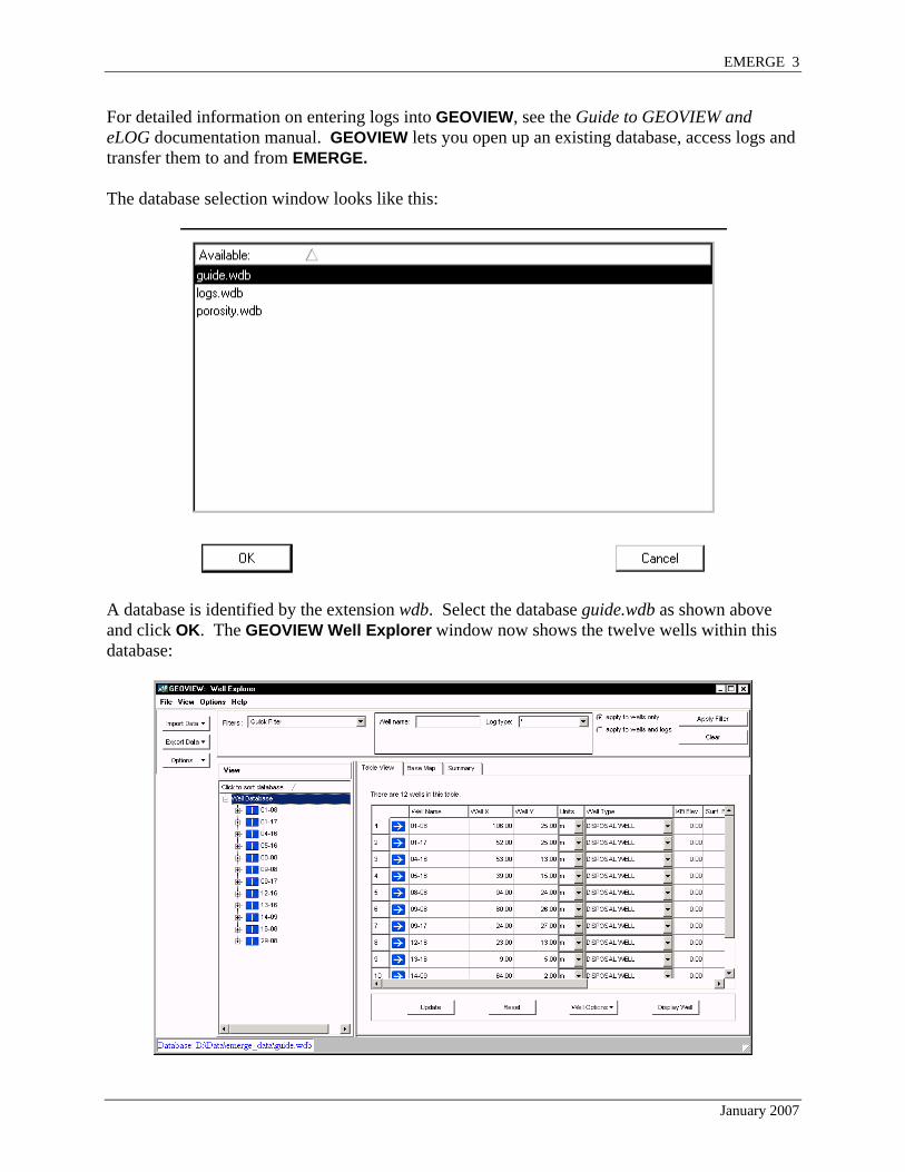
For detailed information on entering logs into GEOVIEW, see the Guide to GEOVIEW and eLOG documentation manual. GEOVIEW lets you open up an existing database, access logs and transfer them to and from EMERGE. The database selection window looks like this:

A database is identified by the extension wdb. Select the database guide.wdb as shown above and click OK. The GEOVIEW Well Explorer window now shows the twelve wells within this database:

January 2007

4 EMERGE

Starting EMERGE Now that the database has been opened in GEOVIEW, we are ready to start the EMERGE program. To do this, click the EMERGE button on the GEOVIEW main window. The following window will appear:

Click OK to Start a New Project. The File Selection window now appears. Fill it in as shown below and click OK (note that we are calling the new project guide):

January 2007

EMERGE 5

The main EMERGE window now appears:

Before starting the EMERGE project, it is a good time to look at the online help feature in EMERGE. If you click the Help button at the top of the main EMERGE window, you will see this pull-down menu:

January 2007

6 EMERGE

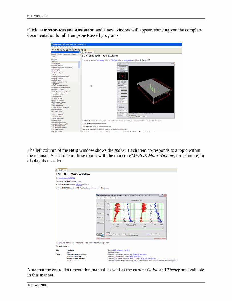
Click Hampson-Russell Assistant, and a new window will appear, showing you the complete documentation for all Hampson-Russell programs:

The left column of the Help window shows the Index. Each item corresponds to a topic within the manual. Select one of these topics with the mouse (EMERGE Main Window, for example) to display that section:

Note that the entire documentation manual, as well as the current Guide and Theory are available in this manner.

January 2007

EMERGE 7

Let us now review the EMERGE process. We wish to use the seismic data to “predict” new sonic logs at every location in the 3D seismic volume. To do this, we will collect some sample data around the well locations and find a relationship between the seismic data at those locations and the measured logs. This step is called “training”. After the training is completed, we will assume that the derived relationship is valid for the entire 3D volume, and apply that relationship to the 3D data set. To start the training process, we will need to read the sonic logs from GEOVIEW into the EMERGE main window. To do this, select Wells>Read From Database. The following window appears:

Notice that this window has a series of pages, which can be viewed by using the Next >> and << Back buttons. You will not be able to click OK until the required pages have been filled in. The first page is the Wells page, which allows us to select which wells to include in the EMERGE analysis. As you can see above, the left column contains all the wells in the guide database. By default, all of the wells are also listed in the right column, meaning that we will use all of them in the training.

January 2007

8 EMERGE

Now click the Next >> button at the bottom of the window. The second page will now appear:

This page is used to tell EMERGE which of the logs in the database is the one that we are trying to predict, i.e., which one is the “Target”. For this guide example, we wish to predict the P-wave (sonic) log, as shown above. Also, we are specifying that, although the log is measured in depth, the analysis (Processing Domain) will be done in Time. This is because the seismic data is measured in time. We need to specify the sample rate correctly (Processing Sample Rate), so that EMERGE can do the depth-to-time conversion properly. Note that the check-shot corrected sonic log will be used for this conversion. When you have filled in the page as shown above, click the Next >> button.

January 2007

EMERGE 9

The third page then appears:

The Tops page allows you to specify the analysis window for training in terms of the tops that have already been entered into the GEOVIEW database. In this project, we have entered four tops: viking, mann, ch_top, and miss. As shown above, select the viking as the start of the analysis window and the miss as the end of the analysis window. Note that the analysis window can be changed later if desired. At this point, the OK button is enabled, indicating that EMERGE has enough data from the GEOVIEW database to proceed. The Next >> button would still be active if the option Predicting Logs From Other Logs had been selected on the first page of this window.

January 2007

10 EMERGE

Now that the entire window has been filled in, click OK. One more confirmation window appears:

The reason this window appears is that for each of the selected wells, there are actually two P-wave logs. One is the original log and the second is the check shot corrected log. By default, the most recently created log will be used. This is the check shot corrected log, which is shown in the table. If you wished to use the other log, clicking on the word P-wave CheckShotCorrected for any of the wells will produce a pull-down menu that allows you to select the desired log. For our case, accept the defaults by clicking OK on this window.

January 2007

EMERGE 11

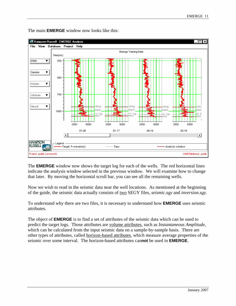
The main EMERGE window now looks like this:

The EMERGE window now shows the target log for each of the wells. The red horizontal lines indicate the analysis window selected in the previous window. We will examine how to change that later. By moving the horizontal scroll bar, you can see all the remaining wells. Now we wish to read in the seismic data near the well locations. As mentioned at the beginning of the guide, the seismic data actually consists of two SEGY files, seismic.sgy and inversion.sgy. To understand why there are two files, it is necessary to understand how EMERGE uses seismic attributes. The object of EMERGE is to find a set of attributes of the seismic data which can be used to predict the target logs. Those attributes are volume attributes, such as Instantaneous Amplitude, which can be calculated from the input seismic data on a sample-by-sample basis. There are other types of attributes, called horizon-based attributes, which measure average properties of the seismic over some interval. The horizon-based attributes cannot be used in EMERGE.

January 2007

12 EMERGE

There is an infinite variety of possible volume attributes. EMERGE contains a list of about 20 attributes which can be calculated internally from the seismic trace. However, many very important volume attributes cannot be calculated internally. One example is a seismic inversion result. This is an attribute of the seismic data, because it has been derived mathematically from the seismic trace. But it is too complex to be calculated within EMERGE itself. A second type of attribute, which cannot be calculated internally, is one that is derived using a proprietary process, such as coherency. To accommodate the possibility of external attributes, EMERGE divides all possible attributes into two categories: Internal Attributes and External Attributes. Internal Attributes are those that EMERGE calculates internally, as required. We will see a list of those attributes shortly. External Attributes are other attributes that have been calculated externally for any reason. External Attributes must be supplied as a separate seismic file. There is no limit to the number of External Attributes supplied, as long as there is a separate seismic file for each External Attribute. Once an External Attribute has been loaded, EMERGE treats both sets of attributes identically. In our guide project, we have one External Attribute, which is an inversion result generated in STRATA. That result is contained in the SEGY file inversion.sgy. Now we will read in the seismic training data. To do this, select Seismic>Add Seismic Input>From File. The following window appears:

January 2007

EMERGE 13

We wish to read both files, inversion.sgy and seismic.sgy. Click Add All >>. The window now looks like this:

Click Next >> on this window. On the next page, you specify that these two files are 3D volumes and that they should be loaded separately.

On the third page, you specify what information can be found in the trace headers. In our case, we do not have either Inline & Xline numbers or X & Y coordinates in the headers. Change the window as shown below:

Click Next >> to see the fourth page.

January 2007

14 EMERGE

The Attribute page is used to provide a name for each of the volumes we are reading into EMERGE. At first it looks like this:

Change the window to look like this:

By making these changes, we have told EMERGE that the volume seismic.sgy is the Raw Seismic data. This means that internal attributes, by default, will be applied to that volume and not the other. The volume inversion.sgy is called an External Attribute. We have given it the name “Inversion Result”, which EMERGE will use to identify it later. There is no limit to the number of attribute volumes which we could add in this way. When you have filled in the page as shown above, click Next >> to get the SEG-Y Format page. The File Format page allows you to specify in detail where many important items are found in the trace headers. Because we have specified that these files use Rectangular geometry, we can default all the items on the page. Click Next >>. This warning message appears, indicating that the two files will now be scanned:

Click Yes on this window to start scanning.

January 2007

EMERGE 15

When the scan is finished, this window appears:

On this window, we specify the geometry of the 3D volume. Note that the only change we needed to make was to set the Number of Cross-lines. Fill in the window as shown above and click OK.

January 2007

16 EMERGE

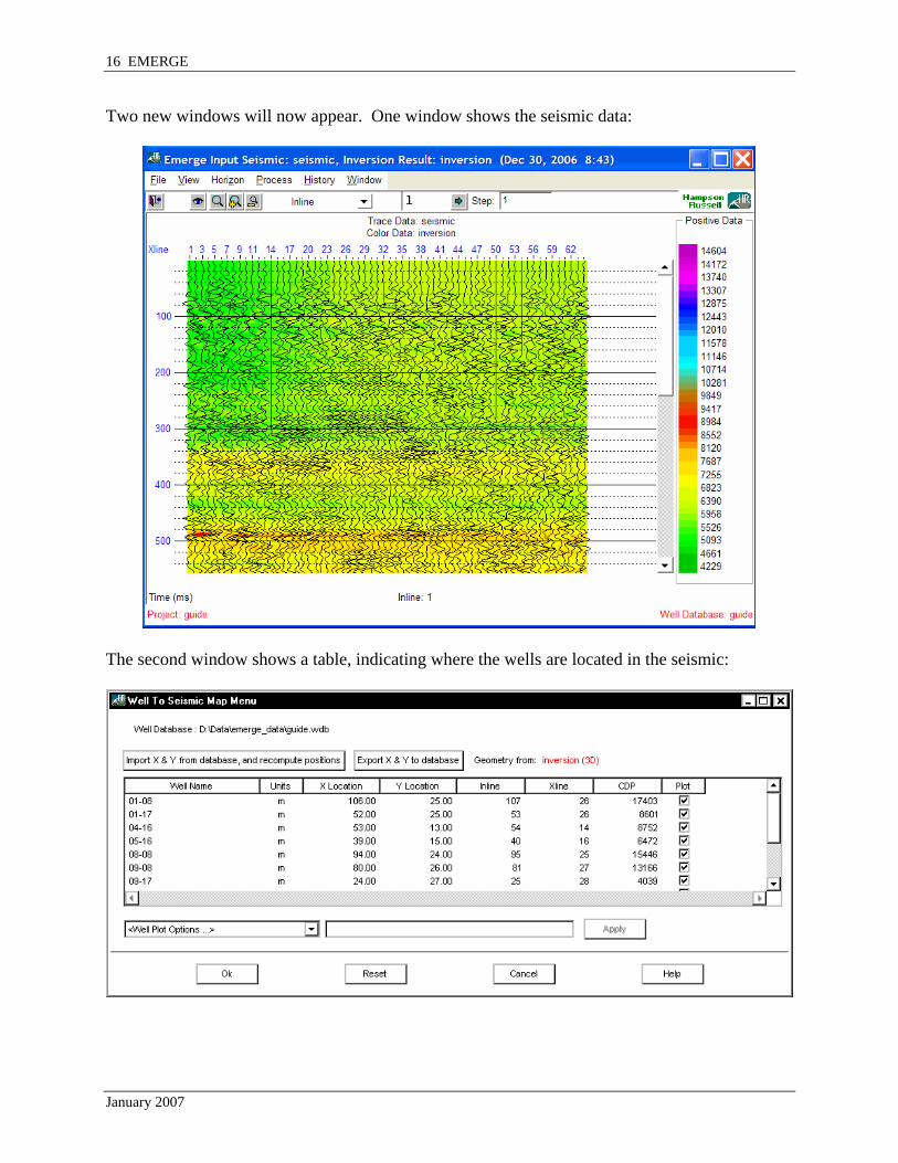
Two new windows will now appear. One window shows the seismic data:

The second window shows a table, indicating where the wells are located in the seismic:

January 2007

EMERGE 17

For this data set, the locations are correct because the X & Y coordinates were entered appropriately in the GEOVIEW database. For other data sets, you may need to modify the Inline and Xline columns of the table. Now, click OK to get this window:

This window tells the EMERGE program how to extract the trace at each well location which is used in the training process. The default is to extract a single trace that follows the trajectory of each of the wells, whether vertical or deviated. Alternatively, you could modify the Capture Option to “Distance”, which will average all traces within a specified distance from each well. In this guide, we will use the Neighbourhood radius value of 1, as shown. This means that the composite trace will be the average of those traces within 1 inline or xline of the well location. This is an average of 9 traces. Click OK.

January 2007

18 EMERGE

The composite trace at each well location will be extracted from the SEGY volumes and the EMERGE main window will be modified to show the additional data:

The EMERGE main window now shows the analysis data for each well: the target log in red, the single seismic trace in black, and the external attribute in blue. Brown horizontal bars also indicate the analysis window. Note that the window may be different from well to well.

January 2007

EMERGE 19

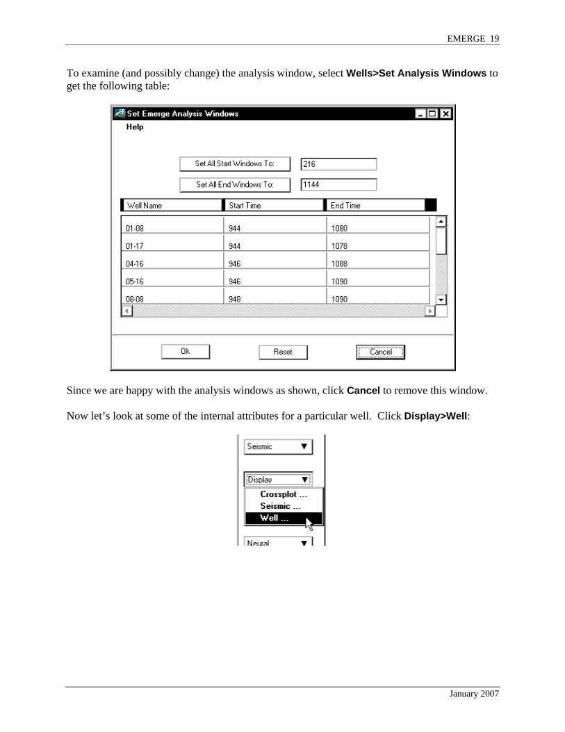
To examine (and possibly change) the analysis window, select Wells>Set Analysis Windows to get the following table:

Since we are happy with the analysis windows as shown, click Cancel to remove this window. Now let’s look at some of the internal attributes for a particular well. Click Display>Well:

January 2007

20 EMERGE

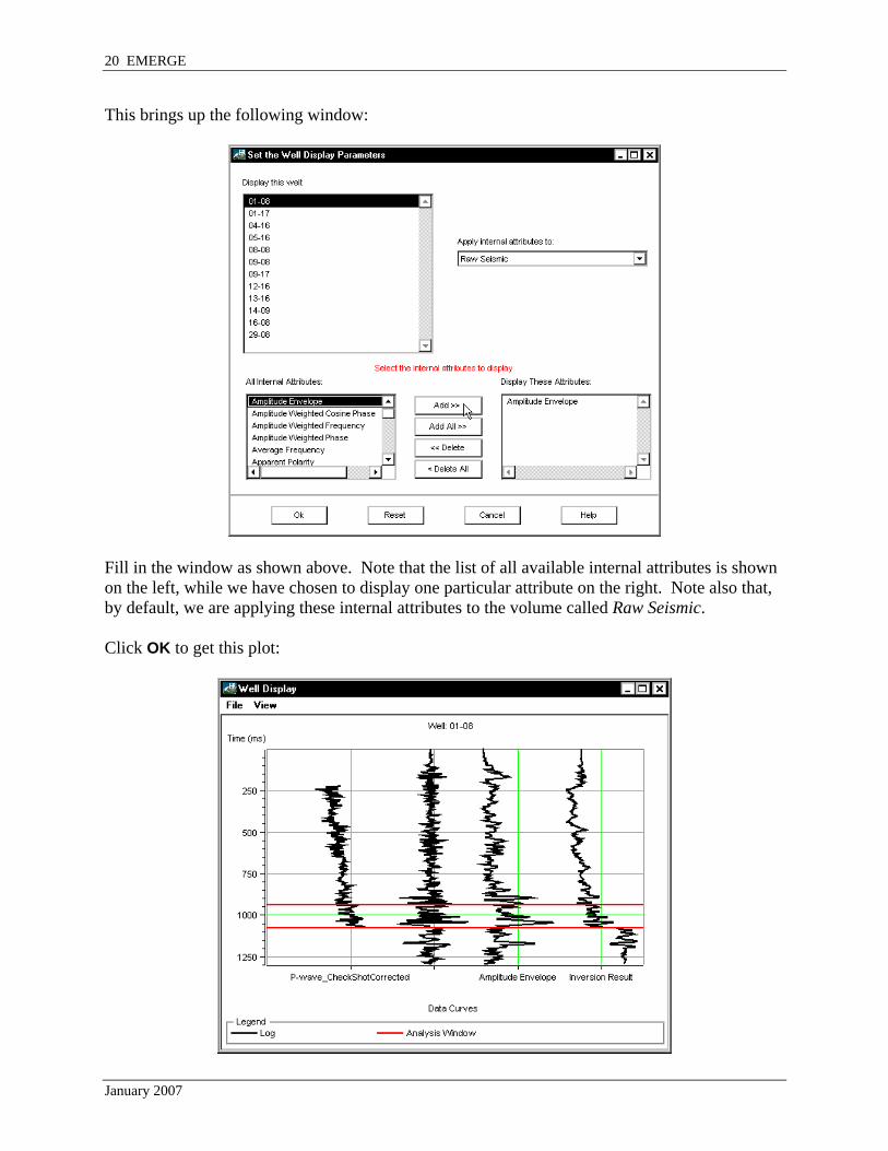
This brings up the following window:

Fill in the window as shown above. Note that the list of all available internal attributes is shown on the left, while we have chosen to display one particular attribute on the right. Note also that, by default, we are applying these internal attributes to the volume called Raw Seismic. Click OK to get this plot:

January 2007

EMERGE 21

To see how well an attribute correlates with the target log, select Display>Crossplot to get this window:

Note that this window will create a cross plot between the target log and any other internal or external attribute. We may use a single well or any combination of wells. In addition, we may apply one of a series of non-linear transforms to the target and/or to the attribute. Fill in the window as shown above, using all wells, and click OK.

January 2007

22 EMERGE

The cross plot appears:

The cross plot has used all points within the analysis windows from all wells. The vertical axis is the target sonic log value, and the horizontal axis is the selected attribute, Inversion Result. A regression curve has been fit through the points and the normalized correlation value of 0.47 has been printed at the top of the display. The normalized correlation is a measure of how useful this attribute is in predicting the target log.

January 2007

EMERGE 23

Performing Single-Attribute Analysis Now let’s calculate the correlation coefficients for all the attributes and rank their values. Click Attribute>Create Single Attribute List to get this window:

The upper left box shows all the wells in the EMERGE project. The upper right box shows the wells to be used in performing this analysis. The default is to use all the wells. The middle left box shows all the attributes (internal and external) in the project. The middle right box shows the attributes to be used in this analysis. Ensure that all the attributes will be used by clicking on Add all >>, as shown above. Note that we have also selected to test whether non-linear transforms applied to either the target log or to the external attributes will enhance the correlation.

January 2007

24 EMERGE

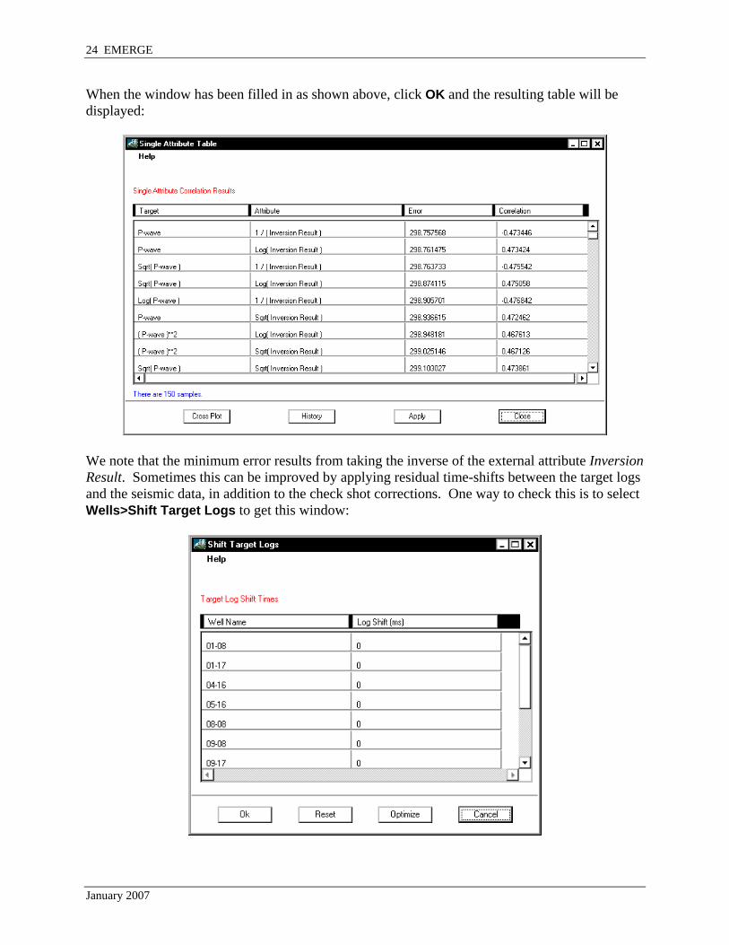
When the window has been filled in as shown above, click OK and the resulting table will be displayed:

We note that the minimum error results from taking the inverse of the external attribute Inversion Result. Sometimes this can be improved by applying residual time-shifts between the target logs and the seismic data, in addition to the check shot corrections. One way to check this is to select Wells>Shift Target Logs to get this window:

January 2007

EMERGE 25

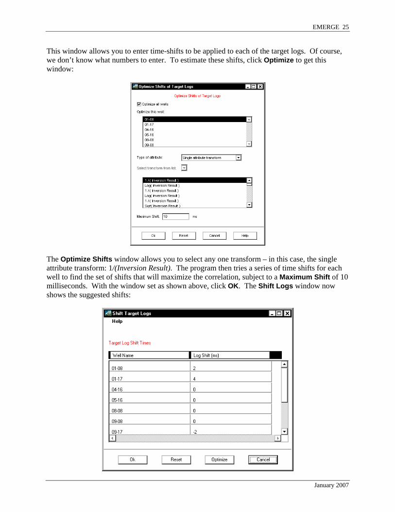
This window allows you to enter time-shifts to be applied to each of the target logs. Of course, we don’t know what numbers to enter. To estimate these shifts, click Optimize to get this window:

The Optimize Shifts window allows you to select any one transform – in this case, the single attribute transform: 1/(Inversion Result). The program then tries a series of time shifts for each well to find the set of shifts that will maximize the correlation, subject to a Maximum Shift of 10 milliseconds. With the window set as shown above, click OK. The Shift Logs window now shows the suggested shifts:

January 2007

26 EMERGE

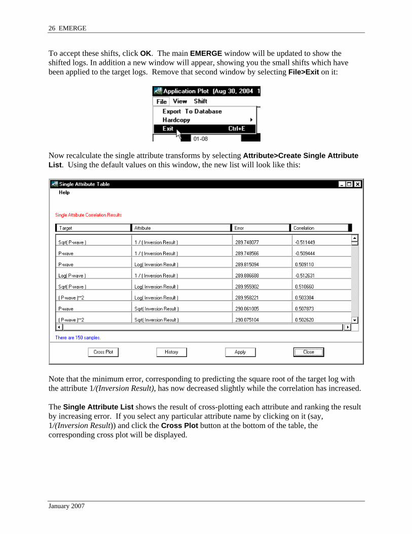
To accept these shifts, click OK. The main EMERGE window will be updated to show the shifted logs. In addition a new window will appear, showing you the small shifts which have been applied to the target logs. Remove that second window by selecting File>Exit on it:

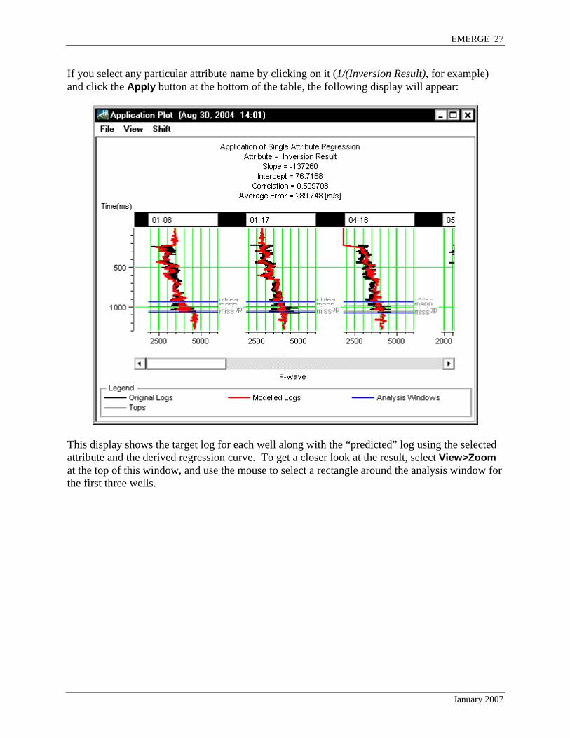
Now recalculate the single attribute transforms by selecting Attribute>Create Single Attribute List. Using the default values on this window, the new list will look like this:

Note that the minimum error, corresponding to predicting the square root of the target log with the attribute 1/(Inversion Result), has now decreased slightly while the correlation has increased. The Single Attribute List shows the result of cross-plotting each attribute and ranking the result by increasing error. If you select any particular attribute name by clicking on it (say, 1/(Inversion Result)) and click the Cross Plot button at the bottom of the table, the corresponding cross plot will be displayed.

January 2007

EMERGE 27

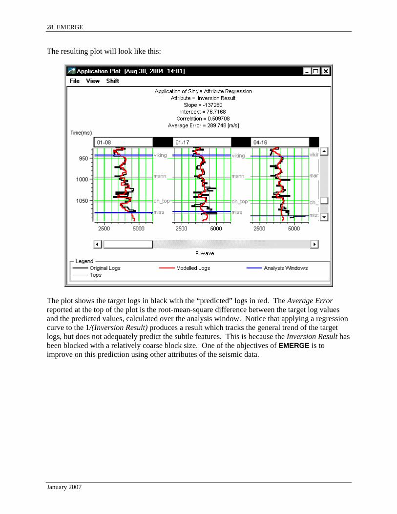
If you select any particular attribute name by clicking on it (1/(Inversion Result), for example) and click the Apply button at the bottom of the table, the following display will appear:

This display shows the target log for each well along with the “predicted” log using the selected attribute and the derived regression curve. To get a closer look at the result, select View>Zoom at the top of this window, and use the mouse to select a rectangle around the analysis window for the first three wells.

January 2007

28 EMERGE

The resulting plot will look like this:

The plot shows the target logs in black with the “predicted” logs in red. The Average Error reported at the top of the plot is the root-mean-square difference between the target log values and the predicted values, calculated over the analysis window. Notice that applying a regression curve to the 1/(Inversion Result) produces a result which tracks the general trend of the target logs, but does not adequately predict the subtle features. This is because the Inversion Result has been blocked with a relatively coarse block size. One of the objectives of EMERGE is to improve on this prediction using other attributes of the seismic data.

January 2007

EMERGE 29

Performing Multi-Attribute Analysis To improve the predictive power, we need to use groups of attributes taken simultaneously. Hopefully, complementary features from several attributes will combine to discriminate subtle features on the target logs, which none of the individuals could predict by themselves. The problem for EMERGE will be to decide which attributes to use and how to weight their importance. To initiate the multi-attribute transform process, select Attribute>Create Multi Attribute List to get this window:

This window contains three pages of parameters, used in the creation of the list of multi-attribute transforms. The first page is used to select which wells will be used in the training. To accept the default, which is to use all the wells, click Next >>.

January 2007

30 EMERGE

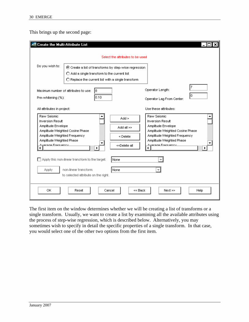
This brings up the second page:

The first item on the window determines whether we will be creating a list of transforms or a single transform. Usually, we want to create a list by examining all the available attributes using the process of step-wise regression, which is described below. Alternatively, you may sometimes wish to specify in detail the specific properties of a single transform. In that case, you would select one of the other two options from the first item.

January 2007

EMERGE 31

An important parameter is Maximum number of attributes to use. In this part of the analysis, EMERGE searches for groups of attributes that can be combined to predict the target. It does this by a process called step-wise regression. This means that it first searches for the single attribute from the list that predicts best by itself. The criterion for evaluating the prediction is the RMS error. In other words, EMERGE tries each attribute, calculates the RMS error, and determines the single best attribute as the one with the lowest error. Having found the single best attribute, EMERGE searches for the best pair of attributes, assuming that one of the pair is the single attribute just found. Once again this is done by trial and error, solving the system of equations as many times as there are other attributes to pair up with the single attribute. Notice that this does not guarantee that the pair found is actually the global best, since it is possible that there is another pair that does not include the single best, but somehow combine in an optimal fashion to predict better. However, the procedure used by EMERGE is much faster than an exhaustive search of all possibilities, and is usually very good. Having found the best pair, EMERGE goes on to look for the best three, the best four, etc. The parameter Maximum number of attributes to use tells EMERGE when to stop looking. This of course affects the run time for the analysis. A second important parameter is the Operator Length. This parameter occurs because EMERGE extends the concept of regression to include convolution. Consider the case of one attribute. Using simple regression, EMERGE assumes that the target samples and the attribute samples are related by this expression:

T(i) = constant + weight x A(i) where T(i) is the target value at sample i and A(i) is the attribute value at sample i

The values of constant and weight are determined by least-squares regression. Actually, since the target is usually a log property and the attribute is usually a seismic property, we expect that a single log sample, i, should be related to a group of neighboring seismic samples around the point i. To accommodate this type of relationship, we can replace the single weight by an operator with some specified length, say 7. Then the expression above becomes convolution instead of multiplication:

T = constant + weight * A where weight is a seven-point operator centered on the target sample.

As before, the weight coefficients are determined by least-squares regression. The parameter Operator Length determines the length of the convolutional operator. Note that a long operator will always predict better than a short one, but there is a danger of predicting the noise. Note also that an Operator Length of 1 is equivalent to conventional regression. A related parameter, the Operator Lag, specifies how the operator is centered with respect to the target sample. The default is to set this equal to 0, which implies that the operator is centered about the application point.

January 2007

32 EMERGE

When the window has been filled in as shown above (change Maximum number of attributes to use to 8, and Operator Length to 7), click OK. This analysis will take several minutes. When it is completed you will see the following table:

The Multi attribute table shows the results of the calculation. Each row corresponds to a particular multi-attribute transform and includes all the attributes above it. For example, the first row, labeled 1/(Inversion Result), tells us that the single best attribute to use alone is 1/(Inversion Result). The second row, Filter 15/20-25/30, actually refers to a transform using both 1/(Inversion Result) and Filter 15/20-25/30 simultaneously, and this is the best pair. As we proceed down the list, we get the best triplet, the best four, etc. The decreasing Error shows that, as expected, the prediction error decreases with increasing number of attributes.

January 2007

EMERGE 33

If you select Error Plot>Versus Attribute Number, the following display appears:

The black (lower) curve shows the prediction error on the vertical axis and the number of attributes on the horizontal axis. Mathematically, this curve should always decrease. It should always be true that adding more attributes will predict the data better. This does not always mean that the added attributes are predicting the true signal in the target log. Eventually, adding more attributes will simply predict the details or “noise” in the log (or in the attributes themselves). Adding more attributes is similar to fitting a higher order polynomial to a set of points. We need a criterion for determining when to stop. The red (upper) curve is the Validation Error and this can help us to decide when we have added too many attributes. Each point in the validation error has been calculated by “hiding” each of the wells and predicting its values using the operator calculated from the other wells. For example, the last red point, corresponding to 8 attributes, has been calculated this way: the 8 attribute types have been arranged according to the table. First Well 1 has been removed from the calculation. The weights for the 8 attributes have been calculated using only Wells 2 to 12. The derived operator was then used to predict the values at Well 1. Since we already know the exact values, the RMS error for Well 1 has been stored. Then Well 2 was hidden and the entire process repeated. The last point on the Validation Curve is the average error for all of the wells calculated this way. It represents the error we could expect if a new well (say, Well 13) was predicted. For this reason, the Validation Curve is a good measure of the validity of the analysis.

January 2007

34 EMERGE

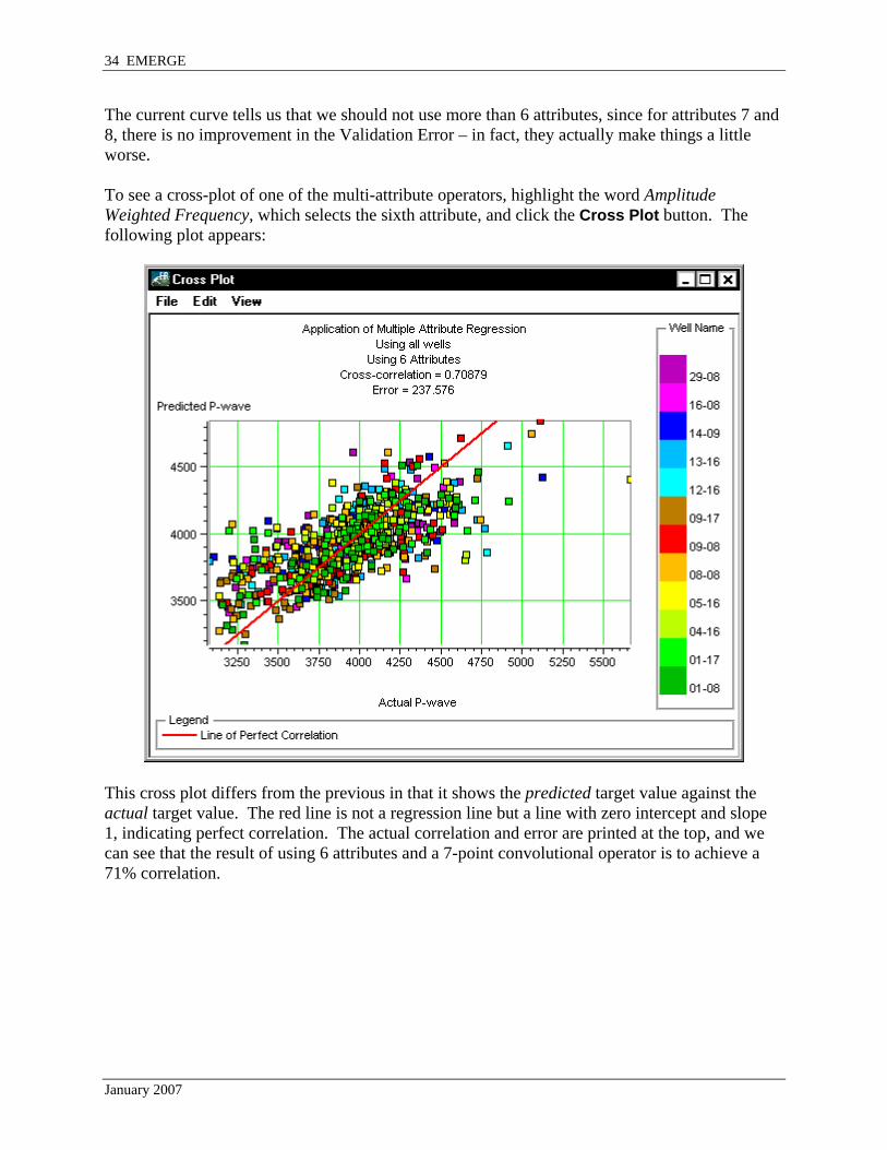
The current curve tells us that we should not use more than 6 attributes, since for attributes 7 and 8, there is no improvement in the Validation Error – in fact, they actually make things a little worse. To see a cross-plot of one of the multi-attribute operators, highlight the word Amplitude Weighted Frequency, which selects the sixth attribute, and click the Cross Plot button. The following plot appears:

This cross plot differs from the previous in that it shows the predicted target value against the actual target value. The red line is not a regression line but a line with zero intercept and slope 1, indicating perfect correlation. The actual correlation and error are printed at the top, and we can see that the result of using 6 attributes and a 7-point convolutional operator is to achieve a 71% correlation.

January 2007

EMERGE 35

Now, highlight the word Amplitude Weighted Frequency, which selects the sixth attribute, and click the List button. The following table appears:

This table lists all the weights for each of the six attributes. Note that there are seven weights for each attribute, because of the seven-point convolutional operator. Now, highlight the word Amplitude Weighted Frequency, which selects the sixth attribute, and select Apply>Training Result. A plot appears, showing the results of applying the multi-attribute transform along with the target logs.

January 2007

36 EMERGE

After using the Zoom option, the plot will look like this:

You may want to compare this result with the prediction using the single attribute. To do that, select Attributes>Display Single Attribute List, select the first single attribute, 1/(Inversion Result), and click Apply. Mathematically, we have increased the correlation from 51% to 71%.

January 2007

EMERGE 37

Another useful display can be seen if you select the sixth row on the multi-attribute transform list (with the name Amplitude Weighted Frequency), and then select Apply>Validation Result:

This display is like the previous one, but as the annotation points out, each predicted log has used an operator calculated from the other wells. For example, the first well, 01-08, used a multi-attribute transform of six attributes whose weights were calculated using only the other 11 wells. The red curve is the predicted value for well 01-08 when it was hidden from the process. Similarly all the other log curves show the calculation when that well is hidden. Effectively, this display shows how well the process will work on a new well, yet to be drilled.

January 2007

38 EMERGE

Applying Attributes to the 3D Volume Now that we have derived the multi-attribute relationship between the seismic and target logs, we will apply the result to the entire 3D volume. To start this, select Display>Seismic. This causes the Seismic Analysis window to appear, if it is not already on the screen:

This window currently shows Inline 1 of the 3D volume. The wiggle traces are the raw seismic data and the color background is the Inversion Result.

January 2007

EMERGE 39

Click View>Parameters to get this window, which allows you to modify the display:

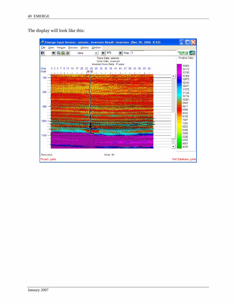
This window can be used to display the data in various forms. For example, by changing the Current Inline to 95, and moving the vertical scroll bar downwards, we can see the sand channel which is the target zone for this data.

January 2007

40 EMERGE

The display will look like this:

January 2007

EMERGE 41

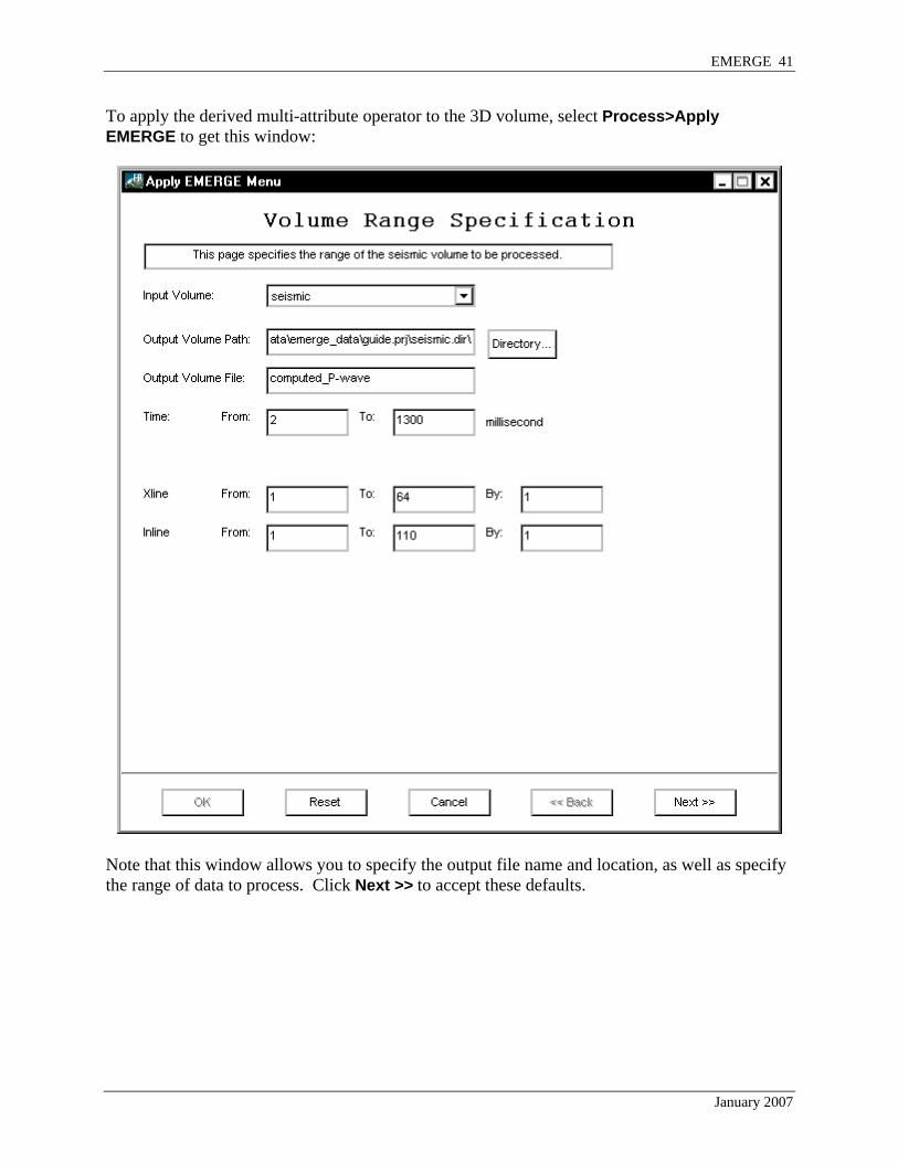
To apply the derived multi-attribute operator to the 3D volume, select Process>Apply EMERGE to get this window:

Note that this window allows you to specify the output file name and location, as well as specify the range of data to process. Click Next >> to accept these defaults.

January 2007

42 EMERGE

The next page appears:

This page specifies which multi-attribute transform we wish to apply. Also, by clicking on Type of transform, you can choose to apply one of the attribute transforms or a Neural Network, if one has been created. We will use this option in the second example in this guide. As with the EMERGE main window, each line in the list is a transform using all of the attributes above it. For example, by selecting Amplitude Weighted Frequency above, we are choosing the transform with 6 attributes. This was the one that the Validation Analysis showed to be the best.

January 2007

EMERGE 43

To examine the parameters used in creating this transform, click History to get the following window:

After selecting Amplitude Weighted Frequency, click Next >> once again to get this window:

January 2007

44 EMERGE

This Output Format window allows you to control the format of the output file. Usually, the defaults are best. Click Next >> once again to get this window:

This page shows all the information that will be stored with the history file, created along with the SEGY file. Note that you can type in your own comments under the field User Description. Now click OK to apply the attribute. The application can take several minutes for the entire 3D volume. While the process is running the following progress monitor appears:

January 2007

EMERGE 45

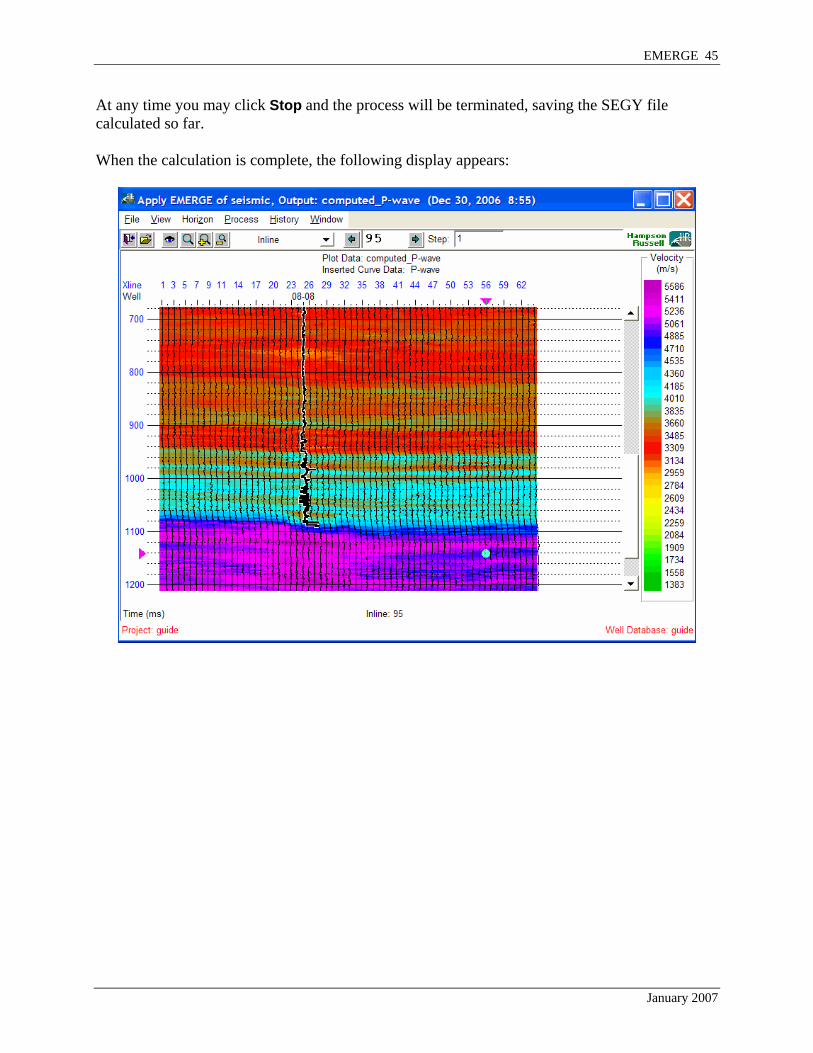
At any time you may click Stop and the process will be terminated, saving the SEGY file calculated so far. When the calculation is complete, the following display appears:

January 2007

46 EMERGE

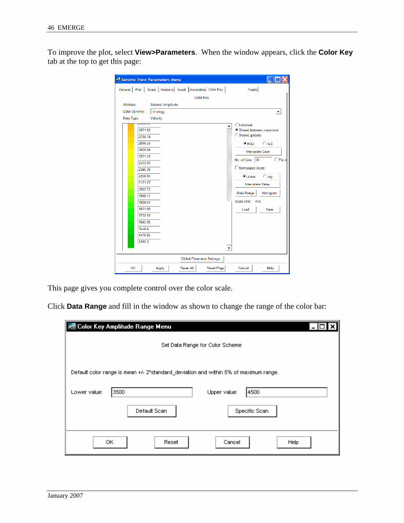
To improve the plot, select View>Parameters. When the window appears, click the Color Key tab at the top to get this page:

This page gives you complete control over the color scale. Click Data Range and fill in the window as shown to change the range of the color bar:

January 2007

EMERGE 47

Then click OK on this window and on the Seismic View Parameters window to get the new display:

Note the channel prominently visible in the center of the display.

January 2007

48 EMERGE

Another interesting way of looking at this result is to produce a data slice. To do this, select Process>Slicing>Create Data Slice on the seismic window showing the computed_P-wave result. The following window appears:

This window allows you to select the volume that you are displaying along with the Plot Attribute. We will use the defaults, so click Next >> to get the following window:

January 2007

EMERGE 49

By filling in this window as shown, we are creating a slice by averaging a 10 ms window centered on the time of 1065 milliseconds. When you have set up the window as shown above, click Next >> and OK to produce this data slice:

The data slice shows a low-velocity channel feature extending horizontally across the survey through many of the wells in the project. Saving the Project Now that the multi-attribute operator has been applied, the last step is to save the current project and all its results. To do this, go back to the EMERGE main window and select Project>Save. After the project has been saved, select File>Exit to close the EMERGE program.

January 2007

50 EMERGE

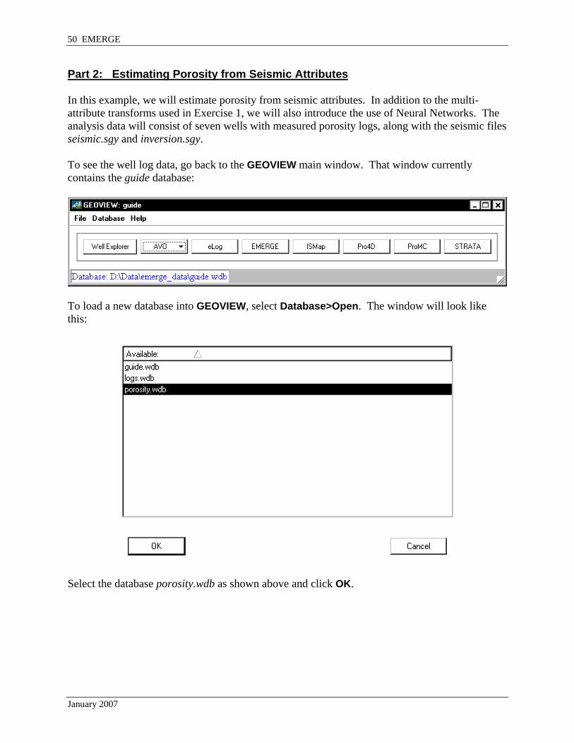
Part 2: Estimating Porosity from Seismic Attributes In this example, we will estimate porosity from seismic attributes. In addition to the multi-attribute transforms used in Exercise 1, we will also introduce the use of Neural Networks. The analysis data will consist of seven wells with measured porosity logs, along with the seismic files seismic.sgy and inversion.sgy. To see the well log data, go back to the GEOVIEW main window. That window currently contains the guide database:

To load a new database into GEOVIEW, select Database>Open. The window will look like this:

Select the database porosity.wdb as shown above and click OK.

January 2007

EMERGE 51

GEOVIEW will now look like this:

Seven wells have now been loaded. To examine the logs within one of the wells, select the well 01-08 from the View table in the GEOVIEW Well Explorer window and click Display Well, to produce the Log Display window:

As you can see, this well contains a porosity log, called den-porosity, along with the other logs.

January 2007

52 EMERGE

Restart the EMERGE program and select Start a New Project. Call the new project porosity as shown below:

The steps for loading the log data into this project are identical to those in Part 1, so they will be summarized briefly here.

January 2007

EMERGE 53

Click Wells>Read From Database and fill in the three pages as shown below:

January 2007

54 EMERGE

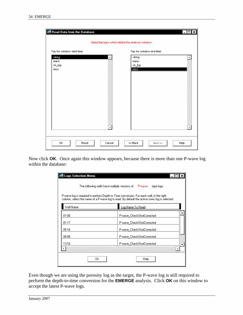
Now click OK. Once again this window appears, because there is more than one P-wave log within the database:

Even though we are using the porosity log as the target, the P-wave log is still required to perform the depth-to-time conversion for the EMERGE analysis. Click OK on this window to accept the latest P-wave logs.

January 2007

EMERGE 55

The EMERGE main window will now look like this, showing the target (porosity) logs:

To load the seismic data, select Seismic>Add Seismic Input>From File and fill in the sequence of pages as shown below. On the first page, select the same input files as in the previous exercise:

Click Next >> to get the next page.

January 2007

56 EMERGE

Set the general information for reading these files. Since we have already read them once, the defaults are now correct:

Identify the volume types and names:

Click Next >> on this and the following page.

January 2007

EMERGE 57

The geometry is correct:

Click OK on this window. After the seismic has been read, set the well-to-seismic mapping (the default is correct):

January 2007

58 EMERGE

Extract the trace at the wells (Use a Neighbourhood radius of 1):

The EMERGE main window now shows the inserted seismic traces:

January 2007

EMERGE 59

The data is now loaded and ready for analysis. The first step is to examine the single-attribute transforms. To do this, select Attribute>Create Single Attribute List to get this window:

Note that we will test non-linear transforms applied to both the target (porosity) and the external attribute (Inversion Result). With the window set as shown above, click OK to get the list:

January 2007

60 EMERGE

We note that the correlations of about 29% are rather poor. One reason for this may be that there are residual time-shifts between the target porosity logs and the seismic data, in spite of the check shot corrections. One way to check this is to select Wells>Shift Target Logs to get this window:

This window allows you to enter time-shifts to be applied to each of the target logs. Of course, we don’t know what numbers to enter. To estimate these shifts, click Optimize to get this window:

January 2007

EMERGE 61

January 2007

62 EMERGE

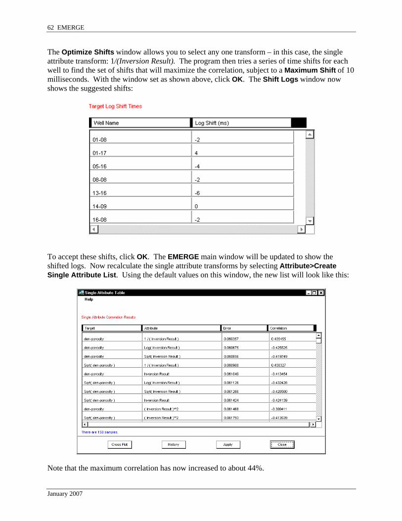
The Optimize Shifts window allows you to select any one transform – in this case, the single attribute transform: 1/(Inversion Result). The program then tries a series of time shifts for each well to find the set of shifts that will maximize the correlation, subject to a Maximum Shift of 10 milliseconds. With the window set as shown above, click OK. The Shift Logs window now shows the suggested shifts:

To accept these shifts, click OK. The EMERGE main window will be updated to show the shifted logs. Now recalculate the single attribute transforms by selecting Attribute>Create Single Attribute List. Using the default values on this window, the new list will look like this:

Note that the maximum correlation has now increased to about 44%.

January 2007

EMERGE 63

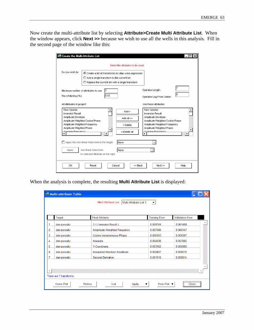
Now create the multi-attribute list by selecting Attribute>Create Multi Attribute List. When the window appears, click Next >> because we wish to use all the wells in this analysis. Fill in the second page of the window like this:

When the analysis is complete, the resulting Multi Attribute List is displayed:

January 2007

64 EMERGE

Click Error Plot>Versus Attribute Number and the Prediction Error Plot appears:

We see that it is best to use six attributes. To see the application, select the sixth row of the Multi-Attribute List (Integrated Absolute Amplitude) and select Apply>Training Result:

January 2007

EMERGE 65

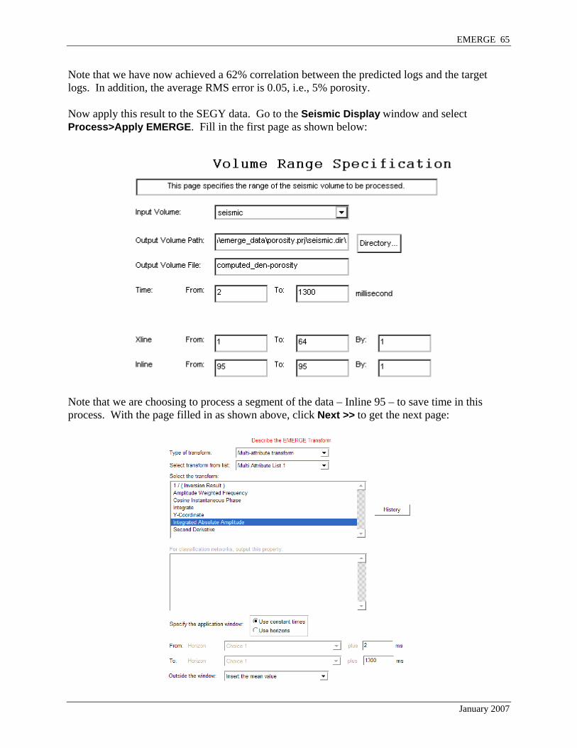
Note that we have now achieved a 62% correlation between the predicted logs and the target logs. In addition, the average RMS error is 0.05, i.e., 5% porosity. Now apply this result to the SEGY data. Go to the Seismic Display window and select Process>Apply EMERGE. Fill in the first page as shown below:

Note that we are choosing to process a segment of the data – Inline 95 – to save time in this process. With the page filled in as shown above, click Next >> to get the next page:

January 2007

66 EMERGE

Select the sixth multi-attribute transform (Integrated Absolute Amplitude), as shown above. Click Next >> and then OK to start the process. When the processing is complete, the computed porosity volume appears:

To improve the display parameters, select View>Parameters. On the Color Key page, change the Color Scheme to Lithology, and uncheck the Normalized Scale parameter:

January 2007

EMERGE 67

To change the numerical range, click Data Range, and set the window as shown:

Click OK on both windows to set the new display of predicted porosity:

Note the predicted high porosity zone at around 1065 ms corresponding to the sand channel from Exercise 1.

January 2007

68 EMERGE

Training Neural Networks In this part of the example, we will use the Neural Network capabilities of EMERGE to improve the porosity prediction. In doing this, we hope that the non-linear characteristics of the Neural Network will increase both the predictive power and the resolution of the derived porosity volume. Under the heading of Neural Network, EMERGE contains four algorithms:

1) Probabilistic (PNN) 2) Multi-layer Feed Forward (MLFN) 3) Discriminant Analysis 4) Radial Basis Function (RBF)

Actually, the Discriminant Analysis algorithm is not strictly a Neural Network, but we have included it in this group because of its classification capabilities. Detailed descriptions of each of these algorithms can be found in the online Theory manual. To see this, select Help>Theory on any of the EMERGE windows. To start the Neural Network analysis, select Neural>Train Neural Network. The following window appears:

We will accept these defaults, which will cause a new network to be created with the name Network_1.

January 2007

EMERGE 69

Click Next >> to get the next page of the window:

As with the multi-attribute training, this page allows us to select the subset of wells to be used in training the Neural Network. The default is to use all the wells. Click Next >> to get the next page:

The question at the top of this page asks if we wish to use one of the previously calculated multi-attribute transforms to structure the Neural Network. Usually, the answer to this is “Yes”.

January 2007

70 EMERGE

This is because the multi-attribute selection process has determined which attributes are best for predicting the target porosity log. By selecting the sixth attribute (called Integrated Absolute Amplitude), we are constructing a Neural Network with precisely the same attributes as those used in that transform. To see the details of that multi-attribute transform, click Show Transform History. With the page filled in as shown above, click Next >> to get this page:

We will start by creating a Probabilistic Neural Network, as shown above. For this network, we will not cascade with the trend from the multi-attribute transform. We will do this in a later example, and the process will be explained then. Finally, by choosing the type of analysis as Mapping, we are specifying that we wish to predict numerical values for the porosity and not classification types.

January 2007

EMERGE 71

Click Next >> to get the final page:

Accept the defaults for the PNN training process by clicking OK. This process will take several minutes, during which the Progress Monitor can be seen:

If you click Stop before the process has completed, you can save the partially trained network. We recommend, however, that you allow the training to finish.

January 2007

72 EMERGE

When the training has been completed, the predicted logs appear:

Note that the correlation of 92% is much higher than that achieved with multi-attribute regression. This is usually the case with Neural Networks because of the non-linear nature of the operator. Note also that the Neural Network has been applied only within the training windows. This is done for two reasons:

(1) The application time for the Neural Network can be very long if applied to the entire window.

(2) The Neural Network is not very good at extrapolating beyond the bounds of the training data. For this reason, it is expected to be less valid outside the training windows than the multi-linear regression.

January 2007

EMERGE 73

After zooming, the result looks like this:

Now we would like to see how the network performs in Validation Mode. This means that we will hide wells and use the trained network to predict their values. To start this, select Neural>Validate Neural Network. The following window appears:

January 2007

74 EMERGE

Click Next >> to select the network which has been trained. The next page appears:

Since all the wells were used for training, only the first selection is appropriate. This means that each of the training wells will be “hidden” in turn and predicted using the remaining wells. Click OK to start this process. When completed, the following plot appears:

January 2007

EMERGE 75

Note that the correlation is now considerably lower (50%). To see how the errors are distributed over the wells, select View>Error Plot. The following plot appears:

The validation curve (in red) suggests that the process might possibly be improved by omitting the first well from this analysis (01-08). If you zoom in closely on that well on the validation display, the result looks like this:

January 2007

76 EMERGE

Looking closely at this display, we can see that the predicted curve has the correct events, but some of them are slightly shifted in time with respect to the real porosity log. Because of the very high frequency prediction, the correlation calculation is very sensitive to the precise depth-to-time calculation, and in fact, this can cause the validation errors to be overly pessimistic for Neural Network calculations. For this reason, we will leave in the well with high validation errors. Another possibility for improving the PNN result is to use the trend from the multi-linear regression calculation. This is sometimes useful because Neural Networks operate best on data with stationary statistics, i.e., data sets without a significant long period trend. Actually, we would expect that the porosity logs in this example do not have a significant trend within the analysis window, so that the network which we have derived is probably already optimal. However, if we were predicting velocity logs, as in the first example, the trend might be more of an issue. To evaluate this option, we will create a new network. Click Neural>Train Neural Network. When the window appears, click Next >> to accept the default new network name:

January 2007

EMERGE 77

On the second page, click Next >> to use all the wells again:

On the third page, click Next >> to use the same multi-attribute transform with six attributes as the basis for this network:

January 2007

78 EMERGE

Finally, on the next page, we come to the parameter which we will change:

Note that we have answered “Yes” to the question:

Do you wish to cascade with the trend from the multi-attribute transform?

The effect of this parameter will be explained below. For now, click Next >> and then OK to start training the new network.

January 2007

EMERGE 79

When the training is completed, the following plot appears:

The first thing you can see is that the low-frequency trend from the target logs has actually been predicted outside the analysis windows. In this mode, the first calculation that the network performs is the multi-linear regression with the same five attributes. The predicted log from that calculation is then smoothed with a smoother length given on the Neural Network training window. The PNN Neural Network is then used to predict the residual, which is the high-frequency component of the logs which is not contained within the smooth trend. The final predicted log is obtained by adding the trend from the multi-linear regression and the predicted residual from the Neural Network. As we can see the correlation is slightly lower than that obtained with the first Neural Network. To calculate the validation error for this network, select Neural>Validate Neural Network.

January 2007

80 EMERGE

On the first page of the window, click Next >> to validate the new network, which has just been created:

On the second page, click OK to begin the validation calculation:

January 2007

EMERGE 81

The new validation result appears:

Note that the correlation of 50% is similar to the validation result for the first network.

January 2007

82 EMERGE

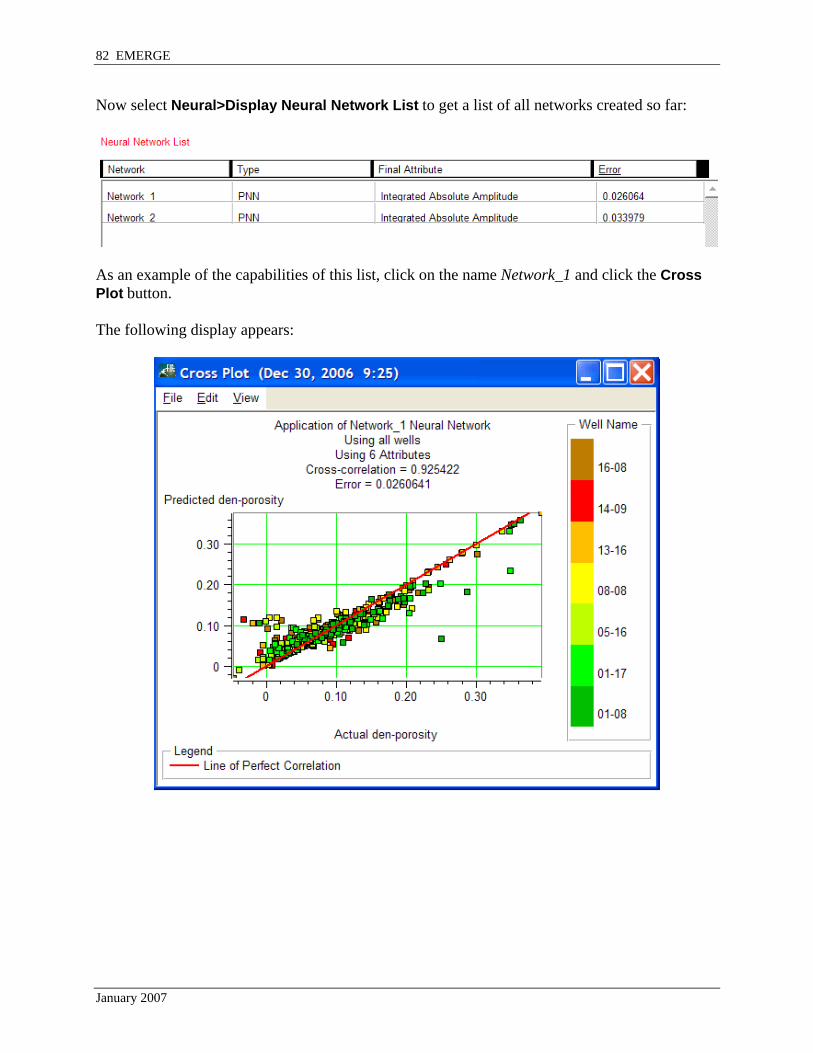
Now select Neural>Display Neural Network List to get a list of all networks created so far:

As an example of the capabilities of this list, click on the name Network_1 and click the Cross Plot button. The following display appears:

January 2007

EMERGE 83

Click the History button to get the detailed history of how this network was created:

January 2007

84 EMERGE

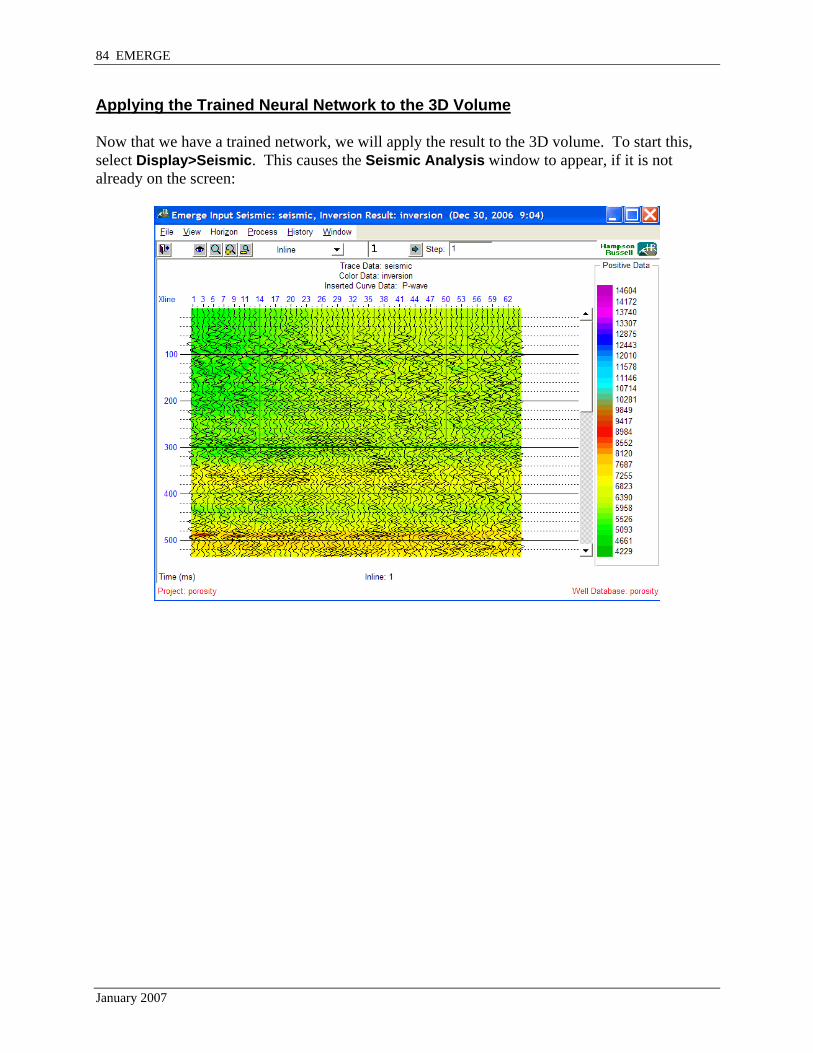
Applying the Trained Neural Network to the 3D Volume Now that we have a trained network, we will apply the result to the 3D volume. To start this, select Display>Seismic. This causes the Seismic Analysis window to appear, if it is not already on the screen:

January 2007

EMERGE 85

Now select Process>Apply EMERGE.

To save time, we will apply the Neural Network operator to a single inline (95). Also, we will create an output SEGY file called pnn_result. When you have completed the page as shown, click Next >> to get this page:

January 2007

86 EMERGE

Note that we have chosen to apply Network_1. Also, because we are applying a Neural Network, the lower part of the page is enabled, allowing us to set an application window for the Neural Network. If horizons had been entered into the project, these could have been used to guide the Neural Network application window. Since there are no horizons, we will apply the network from 1000 to 1200 milliseconds. When the page has been filled in as shown above, click Next >> and OK to start the process. When the calculation has completed, the result appears, but because of the large trace excursion, this plot may be easier to see if the wiggle traces are turned off. To do that, select View>Wiggle Traces: Unshown:

January 2007

EMERGE 87

Select View>Rubberband Zoom, and drag a zoom box across all the traces around the time window where the Neural Network was applied. As before, the high porosity channel can be seen at the well location:

Save this project by selecting Project>Save on the main EMERGE window, and then selecting File>Exit.

January 2007

88 EMERGE

Part 3: Using EMERGE to Predict Logs from Other Logs The first two exercises of this guide have shown how to use EMERGE to predict log data from seismic attributes. An alternate use of the EMERGE program is to predict logs from other logs. In this example, we will predict sonic logs from a series of other log types in the same wells. The data for this example consists of a series of four wells, each containing several log curves. To see this data, go back to the main GEOVIEW window. That window currently contains the porosity database:

To change to the new database, containing the data for this example, select Database>Open. On the Directory Chooser window, select the logs database, as shown below, and click OK:

January 2007

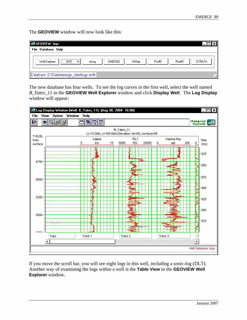
EMERGE 89

The GEOVIEW window will now look like this:

The new database has four wells. To see the log curves in the first well, select the well named B_Yates_11 in the GEOVIEW Well Explorer window and click Display Well. The Log Display window will appear:

If you move the scroll bar, you will see eight logs in this well, including a sonic-log (DLT). Another way of examining the logs within a well is the Table View in the GEOVIEW Well Explorer window.

January 2007

90 EMERGE

The Table View shows the four wells included in the logs database.

From this list, click the blue arrow on the left of the well B_Yates_11 in the Table View, and this list appears:

We can see that this well, B_Yates_11, contains nine logs, including the sonic log and its associated Depth-time table. Examine the other wells, and you will find that one other well, B_Yates_18D, also contains a sonic log, while two of the wells, B_Yates_13 and B_Yates_15 have no sonic logs. The objective of this part of the guide is to predict sonic logs using the other log curves.

January 2007

EMERGE 91

Start the EMERGE program by clicking the EMERGE button on the GEOVIEW main window and select Start a New Project. Call the new project logs, as shown below:

To load the analysis logs from the database, select Wells>Read From Database. When the window appears, all four wells in the database have been selected:

January 2007

92 EMERGE

Select the Predicting Logs From Other Logs option, and click Next >>. The second page should be completed as shown:

Notice that we have selected the P-wave (or sonic) log as the target. Also note that the Processing Domain has been selected as Depth. This is because all the logs are in depth – there is no seismic in this example, so there is no need to convert from depth to time. The Processing Sample Rate must also be set before you can access the next page of this window. When this page of the window is completed as shown above, click Next >> to show the Analysis Window page:

For this example, we have created two tops called Start and End. Select these for the analysis window.

January 2007

EMERGE 93

Then click Next >> to show the External Attributes page:

The list of possible External Attributes shows all of the log curves present in at least one well of the GEOVIEW database. Click Add all >> to select the attributes that will actually be used by EMERGE. You will see two dialogs appear as the database is analyzed. The first informs you that a list of logs is being built, and the second shows the logs that are not found in all four wells. EMERGE will look for a relationship between the remaining six logs and the target sonic log.

January 2007

94 EMERGE

After you click OK, the following window appears:

This is warning us that some of the wells did not have both tops. Click OK to accept this. The main EMERGE window now appears:

By moving the scroll bar, you can see each of the four wells and their associated logs. You will also notice that two of the wells do not contain target logs.

January 2007

EMERGE 95

Now select Display>Crossplot. Fill in the window as shown below:

January 2007

96 EMERGE

The resulting plot looks like this:

Obviously, the P-wave and the Gamma Ray logs show a strong linear relationship with a correlation of 82%. Now go once again to the main EMERGE window and select Display>Crossplot. This time select RILD as the attribute:

January 2007

EMERGE 97

The new cross plot looks like this:

Clearly, this relationship is not linear. Instead, go back to the EMERGE main window once again and select Display>Crossplot. On the window, choose the option to apply the Log transform to both the target (sonic log) and attribute (RILD):

January 2007

98 EMERGE

Now the cross plot looks like this:

This analysis demonstrates that sometimes it helps to apply a non-linear transform to either the target or the attribute or both. Fortunately, EMERGE can help determine which transform to apply.

January 2007

EMERGE 99

To see all the single-attribute transforms, select Attribute>Create Single Attribute List. Fill in the window as shown:

Notice that the Test Non-Linear Transforms of Target and Test Non-Linear Transforms of External Attributes options are checked. This means that for each of the selected External Attributes, Caliper, Gamma Ray, etc., EMERGE will create a series of new attributes by applying a set of non-linear transforms.

January 2007

100 EMERGE

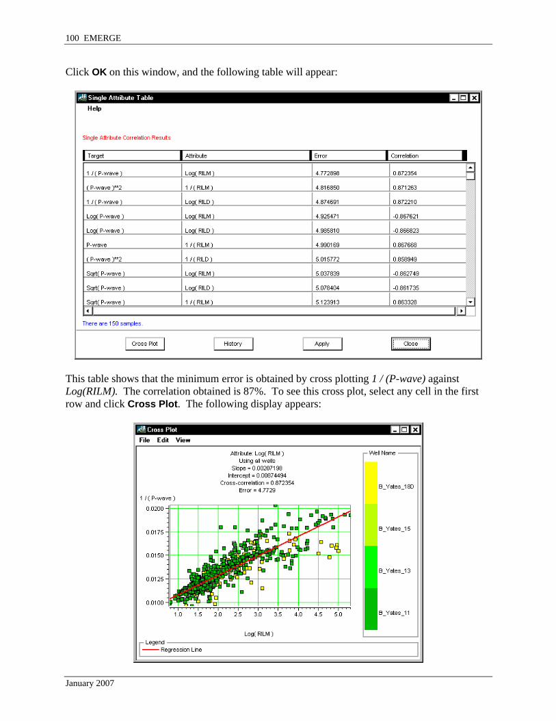
Click OK on this window, and the following table will appear:

This table shows that the minimum error is obtained by cross plotting 1 / (P-wave) against Log(RILM). The correlation obtained is 87%. To see this cross plot, select any cell in the first row and click Cross Plot. The following display appears:

January 2007

EMERGE 101

Now once again, select any cell in the first row and click Apply. The following display appears:

This display shows all four predicted sonic logs in red. Two of the wells, which contain target logs, also show those logs in black.

January 2007

102 EMERGE

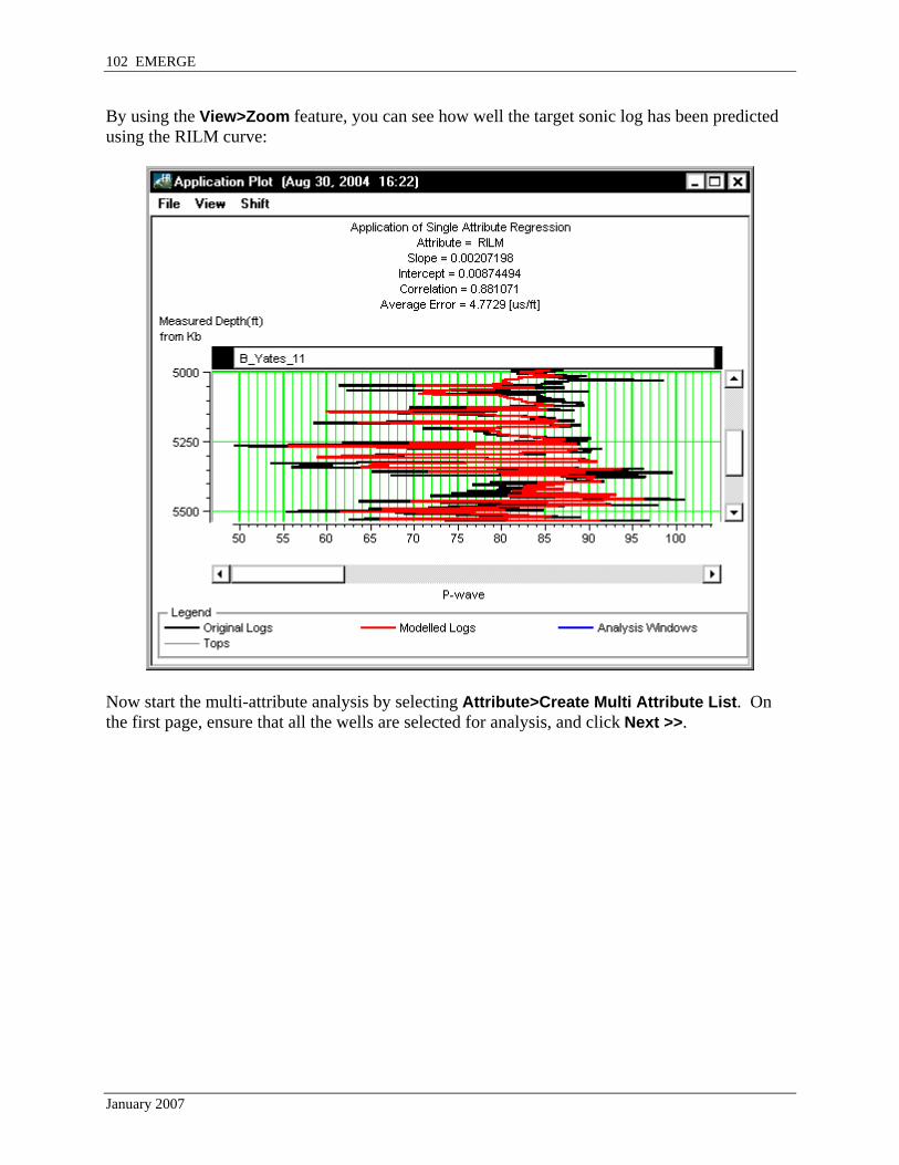
By using the View>Zoom feature, you can see how well the target sonic log has been predicted using the RILM curve:

Now start the multi-attribute analysis by selecting Attribute>Create Multi Attribute List. On the first page, ensure that all the wells are selected for analysis, and click Next >>.

January 2007

EMERGE 103

Fill in the second page as shown below:

Note that for the log prediction from other logs, we tend to use an Operator Length of 1, which is conventional multi-regression. When the analysis is complete the following table appears:

January 2007

104 EMERGE

Just as before, each line on this table represents a multi-attribute transform containing all the attributes down to that line. For example, the third line, with the attribute (Density)**2, represents the multi-attribute transform with Log(RILM), Gamma Ray, and Square of (Density). Click Error Plot>Versus Attribute Number to show the Prediction Error Plot:

As before, the red (upper) curve shows the prediction error for the log that is hidden during the analysis. Clearly, the proper number of attributes to use in this case is three.

January 2007

EMERGE 105

Now, select the third row, with Final Attribute (Density)**2, from the list and click Cross Plot. This display appears:

This plot shows that the correlation between the Predicted and Actual P-wave log is 93%, indicating a very good fit. Now, select the name (Density)**2 (the third attribute) from the list and click List. This table appears:

The table shows the actual weights to be applied to each of the logs in order to predict the sonic log.

January 2007

106 EMERGE

Finally, select the name (Density)**2 (the third attribute) from the list and select Apply>Training Result. This display appears:

On this window, select File>Export To Database. This will cause the predicted logs to be sent back to the GEOVIEW database, where they can be used just like any other log.

January 2007

EMERGE 107

Click Add all >> to export the sonic log from EMERGE to every well in the database.

Click OK on this window. Now the following question appears:

Click No on this window to force the program to calculate new depth-time curves for the new sonic logs we have created.

January 2007

108 EMERGE

To verify that this happened, go back to the Well Explorer window, and click the arrow next to the well B_Yates_11.

In the Table View, you can now see the new log, Emerge_DLT. Click the Display Well button in this window. On the Layout page of the View>Display Options window, uncheck the box labeled Display Only Active Logs, then check the box under the column for Track 2 on the row containing Emerge_DLT, so that the new log will be overlain on the original DLT curve:

January 2007

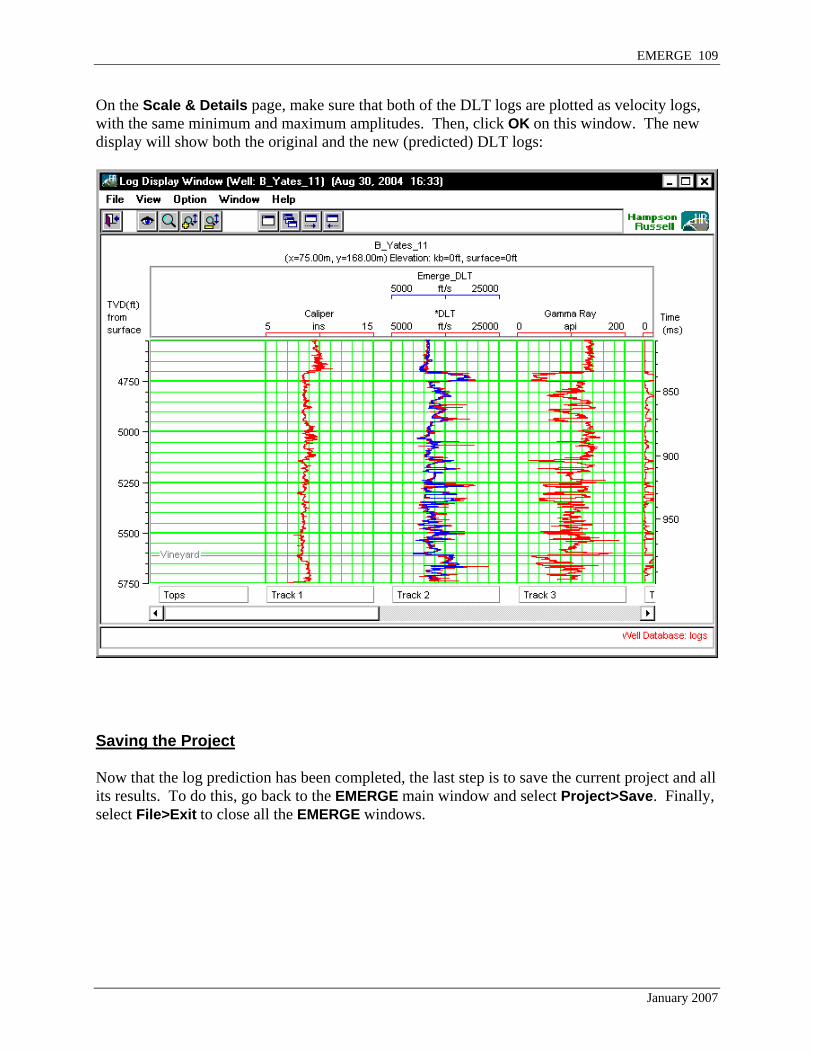
EMERGE 109

On the Scale & Details page, make sure that both of the DLT logs are plotted as velocity logs, with the same minimum and maximum amplitudes. Then, click OK on this window. The new display will show both the original and the new (predicted) DLT logs:

Saving the Project Now that the log prediction has been completed, the last step is to save the current project and all its results. To do this, go back to the EMERGE main window and select Project>Save. Finally, select File>Exit to close all the EMERGE windows.

January 2007