Embedded SystemsLecture 9: Reliability & Fault Tolerance

Björn FrankeUniversity of Edinburgh

Overview

• Definitions

• System Reliability

• Fault Tolerance

Sources and Detection of Errors

Stage Error Sources Error Detection

Specification & DesignAlgorithm Design

Formal SpecificationConsistency Checks

Simulation

PrototypeAlgorithm Design

Wiring & AssemblyTiming Component Failure

Stimulus/Response Testing

ManufactureWiring & AssemblyComponent Failure

System TestingDiagnostics

InstallationAssembly

Component FailureSystem Testing

Diagnostics

Field OperationComponent Failure

Operator ErrorsEnvironmental Factors

Diagnostics

Definitions

• Reliability: Survival Probability

• When function is critical during the mission time.

• Availability: The fraction of time a system meets its specification.

• Good when continuous service is important but it can be delayed or denied

• Failsafe: System fails to a known safe state

• Dependability: Generalisation - System does the right thing at right time

System Reliability

• The reliability, of a system is the probability that no fault of the class F occurs (i.e. system survives) during time t.

where tinit is time of introduction of the system to service,tf is time of occurrence of the first failure f drawn from F.

• Failure Probability, is complementary to

• We can take off the F subscript from and

• When the lifetime of a system is exponentially distributed, the reliability of the system is: where the parameter is called the failure rate

RF (t) = P (tinit ≤ t < tf∀f ∈ F )

RF (t)QF (t)RF (t) + QF (t) = 1

RF (t) QF (t)

R(t) = e−λt λ

RF (t)

Component Reliability Model

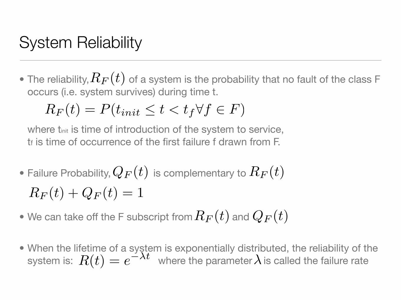
During useful life, components exhibit a constant failure rate λ. Reliability of a device can be modelled using an exponential distributionR(t) = e−λt

Burn In Wear OutUseful Life

Component Failure Rate

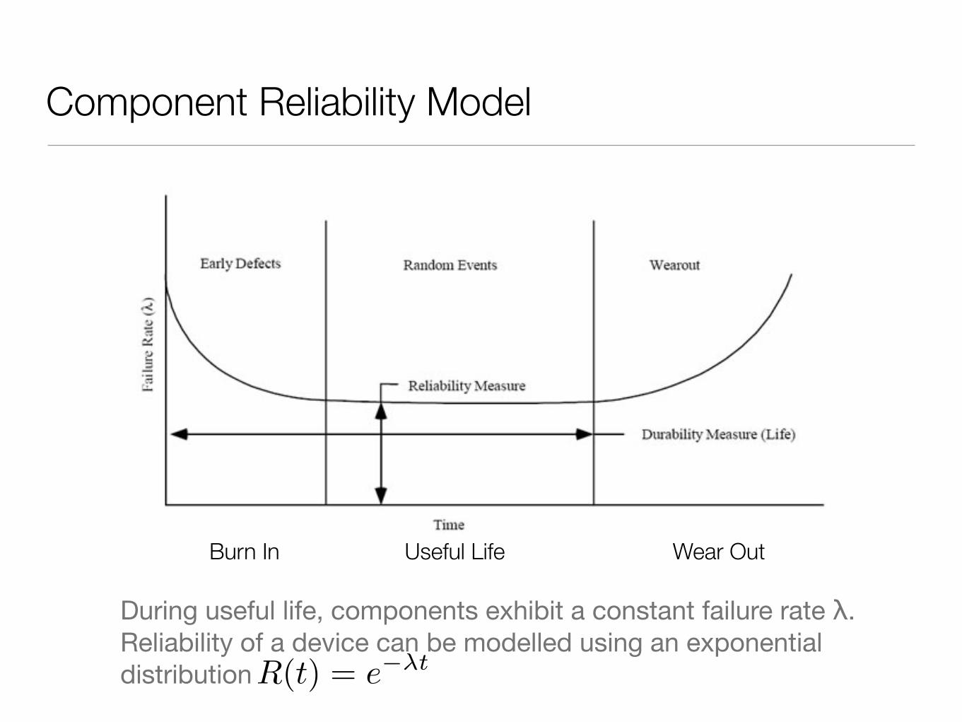
• Failure rates often expressed in failures / million operating hours

Automotive Embedded System Component Failure Rate λ

Military Microprocessor 0.022

Typical Automotive Microprocessor 0.12

Electric Motor Lead/Acid battery 16.9

Oil Pump 37.3

Automotive Wiring Harness (luxury) 775

MTTF: Mean Time To Failure

• MTTF: Mean Time to Failure or Expected Life

• MTTF: Mean Time To (first) Failure is defined as the expected value of tf

where λ is the failure rate.

• MTTF of a system is the expected time of the first failure in a sample of identical initially perfect systems.

• MTTR: Mean Time To Repair is defined as the expected time for repair.

• MTBF: Mean Time Between Failure

MTTF = E(tf ) =� ∞

0R(t)dt =

1λ

MTTF - MTTR - MTBF

Availability = MTBF/(MTBF + MTTR)

Serial System Reliability

• Serially Connected Components

• is the reliability of a single component k:

• Assuming the failure rates of components are statistically independent.

• The overall system reliability

• No redundancy: Overall system reliability depends on the proper working of each component

• Serial failure rate

Rk(t) Rk(t) = e−λkt

Rser(t)Rser(t) = R1(t)×R2(t)×R3(t)× . . .×Rn(t)

Rser(t) =n�

i=1

Ri(t)

Rser(t) = e−t(Pn

i=1 λi)

λser =n�

i=1

λi

System Reliability

• Building a reliable serial system is extraordinarily difficult and expensive.

• For example: if one is to build a serial system with 100 components each of which had a reliability of 0.999, the overall system reliability would be

• Reliability of System of Components

• Minimal Path Set: Minimal set of components whose functioning ensures the functioning of the system: {1,3,4} {2,3,4} {1,5} {2,5}

0.999100 = 0.905

©G.Khan COE718: HW/SW Codesign of Embedded Systems 11

System Reliability Building a reliable serial system is extraordinarily difficult and expensive. For example: if one is to build a serial system with 100

components each of which had a reliability of 0.999, the overall system reliability would be (0.999)100 = 0.905

Reliability of System of Components Minimal Path Set:

Minimal set of components whose functioning ensures the functioning of the system {1,3,4} {2,3,4} {1,5} {2,5}

Parallel System Reliability

• Parallel Connected Components

• is :

• Assuming the failure rates of components are statistically independent.

• Overall system reliability:

Qk(t) 1−Rk(t) Qk(t) = 1− e−λkt

Qpar(t) =n�

i=1

Qi(t)

Rpar(t) = 1−n�

i=1

(1−Ri(t))

Example

• Consider 4 identical modules are connected in parallel

• System will operate correctly provided at least one module is operational. If the reliability of each module is 0.95.

• The overall system reliability is 1− (1− 0.95)4 = 0.99999375

Parallel-Serial Reliability

• Parallel and Serial Connected Components

• Total reliability is the reliability of the first half, in serial with the second half.

• Given R1=0.9, R2=0.9, R3=0.99, R4=0.99, R5=0.87

•

©G.Khan COE718: HW/SW Codesign of Embedded Systems 13

Parallel-Serial Reliability Parallel and Serial Connected Components

Total reliability is the reliability of the first half, in serial with the second half.

Given R1=0.9, R2=0.9, R3=0.99, R4=0.99, R5=0.87 Rt = [1-(1-0.9)(1-0.9)][1-(1-0.87)(1-(0.99*0.99))] = 0.987

Rt = (1− (1− 0.9)(1− 0.9))(1− (1− 0.87)(1− (0.99× 0.99))) = 0.987

Faults and Their Sources

• What is a fault? Fault is an erroneous state of software or hardware resulting from failures of its components

• Fault Sources

• Design errors

• Manufacturing Problems

• External disturbances

• Harsh environmental conditions

• System Misuse

Fault Sources

• Mechanical -- “wears out”

• Deterioration: wear, fatigue, corrosion

• Shock: fractures, overload, etc.

• Electronic Hardware -- “bad fabrication; wears out”

• Latent manufacturing defects

• Operating environment: noise, heat, ESD, electro-migration

• Design defects

• Software -- “bad design”

• Design defects

• “Code rot” -- accumulated run-time faults

• People

• Can take a whole lecture content...

Fault and Classifications

• Failure: Component does not provide service

• Fault: A defect within a system

• Error: A deviation from the required operation of the system or subsystem

• Extent: Local (independent) or Distributed (related)

• Value:

• Determinate

• Indeterminate (varying values)

• Duration:

• Transient

• Intermittent

• Permanent

Fault-Tolerant Computing

• Main aspects of Fault Tolerant Computing (FTC): Fault detection, Fault isolation and containment, System recovery, Fault Diagnosis Repair

©G.Khan COE718: HW/SW Codesign of Embedded Systems 18

Fault-Tolerant Computing Main aspects of FTC: Fault Tolerant Computing

Fault detection Fault isolation and containment System recovery Fault Diagnosis Repair Detection

Time

Diagnosis & Repair

Isolation

Fault

Recovery

td ti

tr

Normal Processing

Switch-in Spare

Time

Tolerating Faults

• There is four-fold categorisation to deal with the system faults and increase system reliability and/or availability.

• Methods for Minimising Faults

• Fault Avoidance: How to prevent the fault occurrence. Increase reliability by conservative design and use high reliability components.

• Fault Tolerance: How to provide the service complying with the specification in spite of faults having occurred or occurring.

• Fault Removal: How to minimise the presence of faults.

• Fault Forecasting: How to estimate the presence, occurrence, and the consequences of faults.

• Fault-Tolerance is the ability of a computer system to survive in the presence of faults.

Fault-Tolerance Techniques

• Hardware Fault Tolerance

• Software Fault Tolerance

Hardware Fault-Tolerance Techniques

• Fault Detection

• Redundancy (masking, dynamic)

• Use of extra components to mask the effect of a faulty component. (Static and Dynamic)

• Redundancy alone does not guarantee fault tolerance. It guarantee higher fault arrival rates (extra hardware).

• Redundancy Management is Important

• A fault tolerant computer can end up spending as much as 50% of its throughput in managing redundancy.

Hardware Fault-Tolerance: Fault Detection

• Detection of a failure is a challenge

• Many faults are latent that show up later

• Fault detection gives warning when a fault occurs.

• Duplication: Two identical copies of hardware run the same computation and compare each other results. When the results do not match a fault is declared.

• Error Detecting Codes: They utilise information redundancy

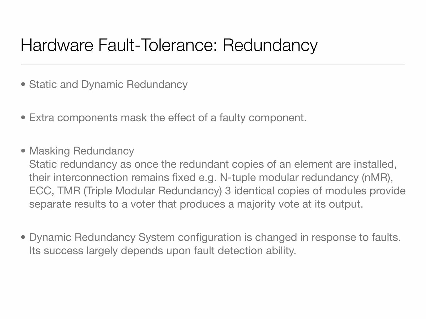
Hardware Fault-Tolerance: Redundancy

• Static and Dynamic Redundancy

• Extra components mask the effect of a faulty component.

• Masking RedundancyStatic redundancy as once the redundant copies of an element are installed, their interconnection remains fixed e.g. N-tuple modular redundancy (nMR), ECC, TMR (Triple Modular Redundancy) 3 identical copies of modules provide separate results to a voter that produces a majority vote at its output.

• Dynamic Redundancy System configuration is changed in response to faults. Its success largely depends upon fault detection ability.

TMR Configuration

• PR1, PR2 and PR3 processors execute different versions of the code for the same application.

• Voter compares the results and forward the majority vote of results (two out of three).

©G.Khan COE718: HW/SW Codesign of Embedded Systems 23

TMR Configuration

PR1, PR2 and PR3 processors execute different versions of the code for the same application. Voter compares the results and forward the majority vote of results (two out of three).

PR3

PR1

PR2

V

Inputs Outputs

Voter

Software Fault-Tolerance

• Hardware based fault-tolerance provides tolerance against physical i.e. hardware faults.

• How to tolerate design/software faults?It is virtually impossible to produce fully correct software.

• We need something:

• To prevent software bugs from causing system disasters. To mask out software bugs.

• Tolerating unanticipated design faults is much more difficult than tolerating anticipated physical faults.

• Software Fault Tolerance is needed as:

• Software bugs will occur no matter what we do. No fully dependable way of eliminating these bugs. These bugs have to be tolerated.

Tolerating Software Failures

• How to Tolerate Software Faults?Software fault-tolerance uses design redundancy to mask residual design faults of software programs.

• Software Fault Tolerance Strategy

• Defensive Programming

• If you can not be sure that what you are doing is correct.

• Do it in many ways.

• Review and test the software.

• Verify the software.

• Execute the specifications.

• Produce programs automatically.

SW Fault-Tolerance Techniques

• Software Fault-tolerance is based on HW Fault-tolerance

• Software Fault Detection is a bigger challenge

• Many software faults are of latent type that shows up later.

• Can use a watchdog to figure out if the program is crashed

• Change the specification to provide low level of service

• Write new versions of the software

• Throw the original version away. Use all the versions and vote the results. N-version Programming (NVP)

• Use an on-line acceptance test to determine which version to believe. Recovery Block Scheme.

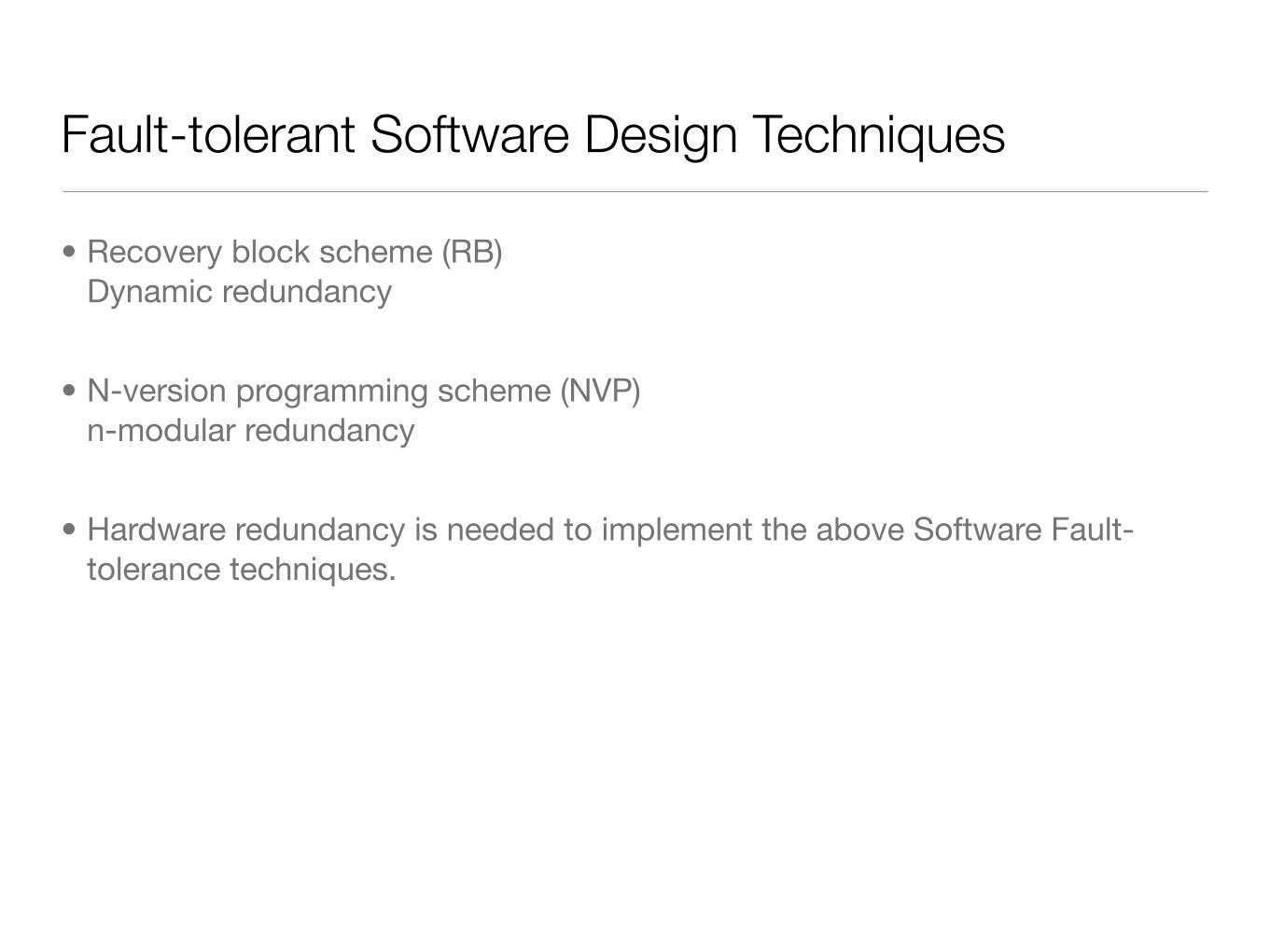
Fault-tolerant Software Design Techniques

• Recovery block scheme (RB)Dynamic redundancy

• N-version programming scheme (NVP)n-modular redundancy

• Hardware redundancy is needed to implement the above Software Fault-tolerance techniques.

Fault-tolerant Software Design Techniques

©G.Khan COE718: HW/SW Codesign of Embedded Systems 29

Software Fault-Tolerance

Fault-tolerant Software Design Techniques

H H

RB

H

V1

H

V2

H

V3

NVP

Primary Primary

Alternate Alternate

N-independent program variants execute in parallel

on the identical input.Results are obtained by

voting upon the output of individual programs

RB Scheme comprises of three elements:

A primary module to execute critical software functions.

Acceptance test for the output of primary module. Alternate modules perform the same

functions as of primary.

Recovery Block Scheme

©G.Khan COE718: HW/SW Codesign of Embedded Systems 32

RB: Recovery Block Scheme An Architectural View of RB

Recovery Memory

Input

Primary

Alternate-1

Alternate-n

Raise error

Rollback and try alternate version Failed

Passed

Failed and alternates exhausted

Output

S w i t c h

AT

RB uses diverse versions Attempt to prevent residual software faults

RB uses diverse versions.Attempt to prevent residual software faults

Fault Recovery

• Fault recovery technique's success depends on the detection of faults accurately and as early as possible.

• Three classes of recovery procedures:

• Full RecoveryIt requires all the aspects of fault tolerant computing.

• Degraded recovery: Also referred as graceful degradation.Similar to full recovery but no subsystem is switched-in.

• Defective component is taken out of service.

• Suited for multiprocessors.

• Safe Shutdown

Fault Recovery

• Two Basic Approaches:

• Forward Recovery

• Produces correct results through continuation of normal processing.

• Highly application dependent

• Backward Recovery

• Some redundant process and state information is recorded with the progress of computation.

• Rollback the interrupted process to a point for which the correct information is available.

• e.g. Retry, Checkpointing, Journaling

Summary

• Reliability

• Serial Reliability, Parallel Reliability, System Reliability

• Fault Tolerance

• Hardware, Software

Preview

• Scheduling Theory

• Priority Inversion

• Priority Inheritance Protocol