Embedded Systems and Programmingjnujprdistance.com/assets/lms/LMS JNU/B.Sc.(IT)/Sem V... · 2019-07-28 · I/JNU OLE Index I. Content .....II II. List of Figures .....VI III. List

Embedded Systems and Programming

This book is a part of the course by Jaipur National University, Jaipur.This book contains the course content for Embedded Systems and Programming.

JNU, JaipurFirst Edition 2013

The content in the book is copyright of JNU. All rights reserved.No part of the content may in any form or by any electronic, mechanical, photocopying, recording, or any other means be reproduced, stored in a retrieval system or be broadcast or transmitted without the prior permission of the publisher.

JNU makes reasonable endeavours to ensure content is current and accurate. JNU reserves the right to alter the content whenever the need arises, and to vary it at any time without prior notice.

I/JNU OLE

Index

ContentI. ...................................................................... II

List of FiguresII. ..........................................................VI

List of TablesIII. ........................................................VIII

AbbreviationsIV. .........................................................IX

Application V. ............................................................ 120

BibliographyVI. ......................................................... 132

Self Assessment AnswersVII. ................................... 135

Book at a Glance

II/JNU OLE

Contents

Chapter I ....................................................................................................................................................... 1Embedded Systems Overview ..................................................................................................................... 1Aim ................................................................................................................................................................ 1Objectives ...................................................................................................................................................... 1Learning outcome .......................................................................................................................................... 11.1 Introduction ............................................................................................................................................. 21.2 Design Challenge – Optimising Design Metrics .................................................................................... 41.3 Embedded Processor Technology ............................................................................................................ 6 1.3.1 General-Purpose Processors -- Software ................................................................................. 6 1.3.2 Single-Purpose Processors -- Hardware .................................................................................. 7 1.3.3 Application-Specific Processors .............................................................................................. 71.4 IC Technology .......................................................................................................................................... 8 1.4.1 Full-Custom/VLSI ................................................................................................................... 9 1.4.2 Semi-Custom ASIC (gate array and standard cell) .................................................................. 9 1.4.3 PLD .......................................................................................................................................... 91.5 Design Technology ................................................................................................................................ 10 1.5.1 Compilation/Synthesis ............................................................................................................11 1.5.2 Libraries/IP ............................................................................................................................ 12 1.5.3 Test/Verification ..................................................................................................................... 12 1.5.4 Other Productivity Improvers ................................................................................................ 12Summary ..................................................................................................................................................... 13References ................................................................................................................................................... 13Recommended Reading ............................................................................................................................. 13Self Assessment ........................................................................................................................................... 14

Chapter II ................................................................................................................................................... 16Overview of Microcontrollers ................................................................................................................... 16Aim .............................................................................................................................................................. 16Objectives .................................................................................................................................................... 16Learning outcome ........................................................................................................................................ 162.1 Introduction ............................................................................................................................................ 172.2 Embedded Controller ............................................................................................................................. 172.3 Microcontrollers and Microprocessors .................................................................................................. 17 2.3.1 Central Processing Unit (CPU) .............................................................................................. 20 2.3.2 Fetching and Executing an Instruction .................................................................................. 20 2.3.3 The Buses: Address, Data, and Control ................................................................................. 20 2.3.4 Control/Monitor (Input/output) Devices ................................................................................ 202.4 Types of Microcontrollers ...................................................................................................................... 21 2.4.1 The 8,16 and 32-Bit Microcontrollers ................................................................................... 212.5 Embedded and External Memory Microcontrollers .............................................................................. 22 2.5.1 Embedded Microcontrollers .................................................................................................. 22 2.5.2 External Memory Microcontrollers ....................................................................................... 222.6 Microcontroller Architectural Features .................................................................................................. 22 2.6.1 Von-Neumann Architecture ................................................................................................... 22 2.6.2 Harvard Architecture .............................................................................................................. 23 2.6.3 CISC (Complex Instruction Set Computer) Architecture Microcontrollers .......................... 23 2.6.4 RISC (Reduced Instruction Set Computer) Architecture Microcontrollers ........................... 24 2.6.5 SISC (Specific Instruction Set Computer) ............................................................................. 242.7 Microcontroller Applications ................................................................................................................. 242.8 Commercial Microcontroller Devices .................................................................................................... 24

III/JNU OLE

Summary ..................................................................................................................................................... 26References .................................................................................................................................................. 26Recommended Reading ............................................................................................................................ 26Self Assessment ........................................................................................................................................... 27

Chapter III .................................................................................................................................................. 29Embedded System Hardware ................................................................................................................... 29Aim .............................................................................................................................................................. 29Objectives .................................................................................................................................................... 29Learning outcome ........................................................................................................................................ 293.1 Introduction ............................................................................................................................................ 303.2 Input ....................................................................................................................................................... 31 3.2.1 Sensors ................................................................................................................................... 31 3.2.2 Sample-and-Hold Circuits ..................................................................................................... 32 3.2.3 A/D-Converters ...................................................................................................................... 323.3 Communication ...................................................................................................................................... 34 3.3.1 Requirements ......................................................................................................................... 34 3.3.2 Guaranteeing Real-time Behaviour ....................................................................................... 363.4 Processing Units..................................................................................................................................... 36 3.4.1 Application-Specific Circuits (ASICs) .................................................................................. 37 3.4.2 Processors .............................................................................................................................. 373.5 Output .................................................................................................................................................... 41 3.5.1 Displays ................................................................................................................................. 41 3.5.2 Electro-mechanical Devices .................................................................................................. 41 3.5.3 Actuators ................................................................................................................................ 43Summary ..................................................................................................................................................... 44References .................................................................................................................................................. 44Recommended Reading ............................................................................................................................. 44Self Assessment ........................................................................................................................................... 45

Chapter IV .................................................................................................................................................. 47Devices and Buses ...................................................................................................................................... 47Aim .............................................................................................................................................................. 47Objectives .................................................................................................................................................... 47Learning outcome ........................................................................................................................................ 474.1 Introduction ........................................................................................................................................... 484.2 I/O Ports- Serial and Parallel Ports ........................................................................................................ 48 4.2.1 Types of Serial Ports .............................................................................................................. 48 4.2.2 Types of Parallel Ports ........................................................................................................... 524.3 Modes of Communication ...................................................................................................................... 53 4.3.1 Communication Protocols ...................................................................................................... 534.4 Timing and Counting Devices ............................................................................................................... 54 4.4.1 Timer ..................................................................................................................................... 54 4.4.2 Counter ................................................................................................................................... 554.5 Serial Bus Communication Protocols .................................................................................................... 55 4.5.1 I2C ......................................................................................................................................... 55 4.5.2 CAN ....................................................................................................................................... 57Summary .................................................................................................................................................... 59References ................................................................................................................................................... 59Recommended Reading ............................................................................................................................. 59Self Assessment ........................................................................................................................................... 60

IV/JNU OLE

Chapter V .................................................................................................................................................... 62Programming Concepts and Embedded Programming in C, C++ ....................................................... 62Aim .............................................................................................................................................................. 62Objectives .................................................................................................................................................... 62Learning outcome ........................................................................................................................................ 625.1 Introduction ............................................................................................................................................ 635.2 Software Programming in Assembly Language (ALP) and in High Level Language C ...................... 63 5.2.1 Assembly Language Programming ........................................................................................ 63 5.2.2 High Level Language ............................................................................................................. 635.3 C, Program Elements: Header and Source Files and Pre-processor Directives ..................................... 63 5.3.1 Include Directive for the Inclusion of Files ........................................................................... 63 5.3.2 Source Files ............................................................................................................................ 64 5.3.3 Pre-processor Directives ........................................................................................................ 645.4 Program Elements .................................................................................................................................. 64 5.4.1 Macros ................................................................................................................................... 64 5.4.2 Functions ................................................................................................................................ 65 5.4.3 Use of Data Types .................................................................................................................. 65 5.4.4 Use of Data Structures ........................................................................................................... 65 5.4.4.1 Queue ...................................................................................................................... 66 5.4.4.2 Stack ........................................................................................................................ 66 5.4.4.3 Array (One Dimensional Vector) ............................................................................. 66 5.4.4.4 Tree .......................................................................................................................... 67 5.4.5 Use of Modifiers .................................................................................................................... 67 5.4.6 Use of Conditions, Loops and Infinite Loops ........................................................................ 67 5.4.7 Use of Pointers ....................................................................................................................... 68 5.4.7.1 NULL Pointer .......................................................................................................... 68 5.4.8 Use of Function Calls ............................................................................................................ 685.5 Embedded Programming In C++ ........................................................................................................... 69 5.5.1 Objected Oriented Programming ........................................................................................... 69 5.5.2 Embedded Programming in C+ + .......................................................................................... 71Summary .................................................................................................................................................... 73References .................................................................................................................................................. 73Recommended Reading ............................................................................................................................. 73Self Assessment ........................................................................................................................................... 74

Chapter VI .................................................................................................................................................. 76Standard Software: Embedded Operating Systems, Middleware, and Scheduling ............................ 76Aim .............................................................................................................................................................. 76Objectives .................................................................................................................................................... 76Learning outcome ........................................................................................................................................ 766.1 Introduction ........................................................................................................................................... 776.2 Prediction of Execution Times ............................................................................................................... 776.3 Scheduling in Real-Time Systems ......................................................................................................... 78 6.3.1 Classification of Scheduling Algorithms ............................................................................... 78 6.3.2 Aperiodic Scheduling ............................................................................................................. 80 6.3.3 Scheduling with Precedence Constraints ............................................................................... 83 6.3.4 Periodic Scheduling ............................................................................................................... 84 6.3.5 Resource Access Protocols .................................................................................................... 87Summary .................................................................................................................................................... 90References ................................................................................................................................................... 90Recommended Reading ............................................................................................................................. 90Self Assessment ........................................................................................................................................... 91

V/JNU OLE

Chapter VII ................................................................................................................................................ 93Basic Concepts of Real Time Operating Systems ................................................................................... 93Aim .............................................................................................................................................................. 93Objectives .................................................................................................................................................... 93Learning outcome ........................................................................................................................................ 937.1 Introduction ............................................................................................................................................ 947.2 Characteristics of Real-Time Tasks ....................................................................................................... 947.3 Real-Time Scheduling ............................................................................................................................ 977.4 Operating System Designs ..................................................................................................................... 977.5 Library-Based RTOS (“Kernel-Less” Approach) .................................................................................. 98 7.5.1 Monolithic Kernels ................................................................................................................ 99 7.5.2 Microkernels .......................................................................................................................... 99 7.5.3 Virtual Machines and Exokernels ........................................................................................ 1017.6 RTOS for Safety Critical Systems ....................................................................................................... 1027.7 Protection in Time Domain .................................................................................................................. 1027.8 Protection in Space Domain ................................................................................................................. 1027.9 Secure Operating System Architecture ................................................................................................ 102Summary .................................................................................................................................................. 104References ................................................................................................................................................. 104Recommended Reading ........................................................................................................................... 104Self Assessment ........................................................................................................................................ 105

Chapter VIII ............................................................................................................................................. 107Validation ................................................................................................................................................. 107Aim ............................................................................................................................................................ 107Objectives .................................................................................................................................................. 107Learning outcome ...................................................................................................................................... 1078.1 Introduction .......................................................................................................................................... 1088.2 Simulation ............................................................................................................................................ 1088.3 Rapid Prototyping and Emulation ........................................................................................................ 1098.4 Test ....................................................................................................................................................... 1098.5 Fault Simulation ....................................................................................................................................1128.6 Fault Injection .......................................................................................................................................1138.7 Risk and Dependability Analysis ..........................................................................................................1138.8 Formal Verification ...............................................................................................................................114Summary ...................................................................................................................................................117References ..................................................................................................................................................117Recommended Reading ............................................................................................................................117Self Assessment ..........................................................................................................................................118

VI/JNU OLE

List of Figures

Fig. 1.1 An embedded system example -- a digital camera ........................................................................... 3Fig. 1.2 Design metric competition -- decreasing one may increase others .................................................. 4Fig. 1.3 Market window ................................................................................................................................. 5Fig. 1.4 IC capacity exponential increase ...................................................................................................... 5Fig. 1.5 Processors very in their customization for the problem at hand:

(a) desired functionality, (b) general-purpose processor, (b) application-specific processor, (c) single-purpose processor ............................................................................................................. 6

Fig. 1.6 Implementing desired functionality on different processor types: (a) general-purpose, (b) application-specific, (c) single-purpose ..................................................... 7

Fig. 1.7 A simplified CMOS transistor .......................................................................................................... 8Fig. 1.8 The independence of processor and IC technologies ....................................................................... 9Fig. 1.9 Ideal top-down design process and productivity improvers ........................................................... 10Fig. 1.10 The co-design ladder: recent maturation of synthesis enables a

unified view of hardware and software ........................................................................................11Fig. 2.1 General block diagram of CPU (Microprocessor) .......................................................................... 18Fig. 2.2 Microcomputer block diagram ....................................................................................................... 18Fig. 2.3 A block diagram of a microcontroller ............................................................................................. 19Fig. 2.4 Types of Microcontrollers ............................................................................................................... 21Fig. 2.5 Von-Neumann architecture block diagram ..................................................................................... 22Fig. 2.6 Harvard architecture block diagram ............................................................................................... 23Fig. 3.1 Simplified design information flow ................................................................................................ 30Fig. 3.2 Hardware in the loop ...................................................................................................................... 30Fig. 3.3 Acceleration sensor ......................................................................................................................... 31Fig. 3.4 Sample-and-hold-circuit ................................................................................................................. 32Fig. 3.5 Flash A/D converter ........................................................................................................................ 33Fig. 3.6 Successive approximation .............................................................................................................. 33Fig. 3.7 Single-ended signalling .................................................................................................................. 35Fig. 3.8 Differential signalling ..................................................................................................................... 35Fig. 3.9 Number of operations per Watt ....................................................................................................... 36Fig. 3.10 Dynamic power management states of the StrongArm Processor SA 1100 ................................. 38Fig. 3.11 Decompression of compressed instructions .................................................................................. 39Fig. 3.12 Re-encoding THUMB into ARM instructions .............................................................................. 40Fig. 3.13 Dictionary approach for instruction compression ........................................................................ 40Fig. 3.14 D/A-converter ............................................................................................................................... 41Fig. 4.1 Types of serial ports ........................................................................................................................ 48Fig. 4.2 Synchronous serial input device ..................................................................................................... 49Fig. 4.3 Synchronous serial output device ................................................................................................... 50Fig. 4.4 Asynchronous serial output ........................................................................................................... 51Fig. 4.5 Types of parallel ports .................................................................................................................... 52Fig. 4.6 Serial bus controller for I2C in a microcontroller .......................................................................... 55Fig. 4.7 I2C bus ............................................................................................................................................ 56Fig. 4.8 Serial bus controller for CAN in a microcontroller ........................................................................ 57Fig. 6.1 Simplified design information flow ................................................................................................ 77Fig. 6.2 Classes of scheduling algorithms ................................................................................................... 78Fig. 6.3 Task descriptor list in a TT operating system ................................................................................. 79Fig. 6.4 Definition of the laxity of a task ..................................................................................................... 81Fig. 6.5 EDF schedule .................................................................................................................................. 81Fig. 6.6 Least laxity schedule ...................................................................................................................... 82Fig. 6.7 Scheduler needs to leave processor idle ......................................................................................... 82Fig. 6.8 Precedence graph and schedule ...................................................................................................... 83Fig. 6.9 Notation used for time intervals ..................................................................................................... 84Fig. 6.10 Right hand side of equation 6.5 .................................................................................................... 85Fig. 6.11 Example of a schedule generated with RM scheduling ................................................................ 85

VII/JNU OLE

Fig. 6.12 RM schedule does not meet deadline at time ............................................................................... 86Fig. 6.13 EDF generated schedule for the example of 6.12 ......................................................................... 86Fig. 6.14 Priority inversion for two tasks .................................................................................................... 87Fig. 6.15 Priority inversion with potentially large delay ............................................................................. 88Fig. 6.16 Priority inheritance ...................................................................................................................... 88Fig. 7.1 Parameters of a real-time task ........................................................................................................ 95Fig. 7.2 (a) Execution modes (b) Application binary interface .................................................................... 98Fig. 7.3 Unstructured vs. structured monolithic kernel ............................................................................... 99Fig. 7.4 Microkernel architecture ............................................................................................................... 100Fig. 7.5 Client/Server IPC .......................................................................................................................... 100Fig. 7.6 Virtual machine monitor ............................................................................................................... 101Fig. 7.7 Efficiency classification of ISAs .................................................................................................. 101Fig. 7.8 OS architecture for safety critical systems ................................................................................... 103Fig. 8.1 Simplified design information flow .............................................................................................. 108Fig. 8.2 Scan path design ............................................................................................................................110Fig. 8.3 BILBO............................................................................................................................................111Fig. 8.4 Segment from processor hardware ................................................................................................112Fig. 8.5 Fault tree ........................................................................................................................................114Fig. 8.6 Inputs for model checking .............................................................................................................115

VIII/JNU OLE

List of Tables

Table 2.1 Different types of commercial microcontroller devices ............................................................... 25Table 8.1 Mod es of BILBO .......................................................................................................................111

IX/JNU OLE

Abbreviations

ALU - Arithmetic Logic Unit API - Application Programming Interface ASIC - Application-Specific ICASIP - Application-Specific Instruction-Set Processor BILBO - Built-In Logic Block Observer CCDs - Charge Coupled Devices CISC - Complex Instruction Set ComputerCMOS - Complementary Metal Oxide SemiconductorCRC - Cyclic Redundancy Check CSMA/CA - Carrier-Sense Multiple Access/ Collision AvoidanceCSMA/CD - Carrier-Sense Multiple Access/Collision Detect DMA - Direct Memory AccessDREAMS - Distributed Real-time Extensible Application Management SystemDSPs - Digital-Signal Processors EPROM/PROM/ROM - Erasable Programmable Read Only MemoryFPGA - Field Programmable Gate ArrayHDL - Hardware Description Language IR - Instruction Register ISA - Industry Standard ArchitectureJPEG - Joint Photographic Experts GroupLCD - Liquid Crystal DisplayLFSR - Linear-Feedback Shift Register LIFO - Last In First OutLL - Least Laxity LST - Least Slack Time First MLF - Minimum Laxity FirstPAL - Programmable Array LogicPIC - Programmable Interrupt ControllerPLD - Programmable Logic DevicePSW - Program Status Word RAM - Random Access MemoryRISC - Reduced Instruction Set ComputerRTOS - Real-time Operating System SISC - Specific Instruction Set ComputerTDL - Task-Descriptor List UART - Universal Asynchronous Receiver/Transmitter VLSI - Very Large Scale IntegrationWCET - Worst-Case Execution Time

1/JNU OLE

Chapter I

Embedded Systems Overview

Aim

The aim of this chapter is to:

introduce embedded processor technology•

elucidate general-purpose processors - software•

explain IC technology•

Objectives

The objectives of this chapter are to:

explain single-purpose processors - hardware•

explicate programmable logic device•

elucidate compilation/synthesis•

Learning outcome

At the end of this chapter, you will be able to:

understand design technology•

identifyapplication-specificprocessors•

recognise IC tech• nology


2/JNU OLE

1.1 Introduction Computing systems are everywhere. It’s probably no surprise that millions of computing systems are built every year destined for desktop computers (Personal Computers, or PC’s), workstations, mainframes and servers. What may be surprising is that billions of computing systems are built every year for a very different purpose: they are embedded within larger electronic devices, repeatedly carrying out a particular function, often going completely unrecognisedbythedevice’suser.Creatingaprecisedefinitionofsuchembeddedcomputingsystems,orsimplyembeddedsystems,isnotaneasytask.Wemighttrythefollowingdefinition:Anembeddedsystemisnearlyanycomputingsystemotherthanadesktop,laptop,ormainframecomputer.Thatdefinitionisn’tperfect,butitmaybe as close as we’ll get. We can better understand such systems by examining common examples and common characteristics. Such examination will reveal major challenges facing designers of such systems.

Embedded systems are found in a variety of common electronic devices, such as: Consumer electronics: Cell phones, pagers, digital cameras, camcorders, videocassette recorders, portable video •games, calculators, and personal digital assistants; Home appliances: Microwave ovens, answering machines, thermostat, home security, washing machines, and •lighting systemsOfficeautomation:Faxmachines,copiers,printers,andscanners;•Business equipment: Cash registers, curbside check-in, alarm systems, card readers, product scanners, and •automated teller machinesAutomobiles: Transmission control, cruise control, fuel injection, anti-lock brakes, and active suspension.•

One might say that nearly any device that runs on electricity either already has, or will soon have, a computing system embedded within it. While about 40% of American households had a desktop computer in 1994, each household had an average of more than 30 embedded computers, with that number expected to rise into the hundreds by the year 2000. The electronics in an average car cost $1237 in 1995, and may cost $2125 by 2000. Several billion embedded microprocessor units were sold annually in recent year compared to a few hundred million desktop microprocessor units.

Embedded systems have several common characteristics:Single-functioned: An embedded system usually executes only one program, repeatedly. For example, a pager is •always a pager. In contrast, a desktop system executes a variety of programs, like spreadsheets, word processors, and video games, with new programs added frequently.Tightly constrained: All computing systems have constraints on design metrics, but those on embedded systems •can be especially tight. A design metric is a measure of an implementation’s features, such as cost, size, performance,andpower.Embeddedsystemsoftenmustcostjustafewdollars,mustbesizedtofitonasinglechip, must perform fast enough to process data in real-time, and must consume minimum power to extend battery life or prevent the necessity of a cooling fan.

3/JNU OLE

Microcontroller

CCD preprocessor Pixel coprocessorA/D D/A

JPEG codec

DMA controller

Memory controller ISA bus interface UART LCD ctrl

Display ctrl

Multiplier/Accum

Digital camera

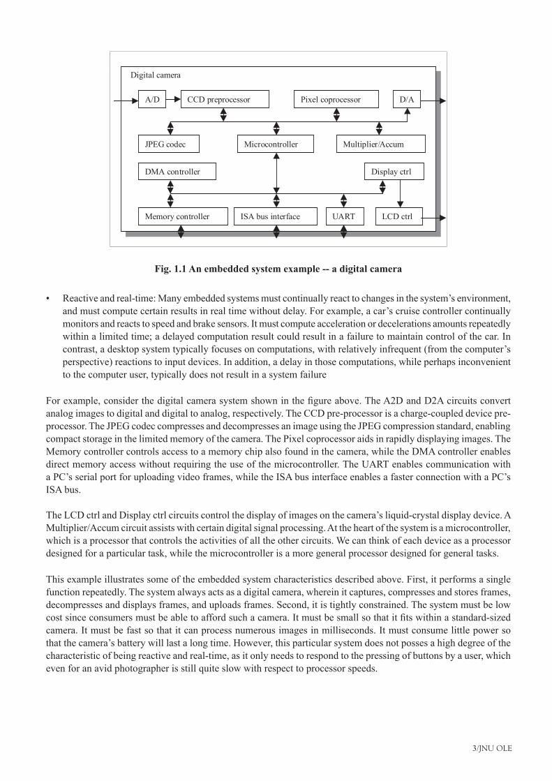
Fig. 1.1 An embedded system example -- a digital camera

Reactive and real-time: Many embedded systems must continually react to changes in the system’s environment, •and must compute certain results in real time without delay. For example, a car’s cruise controller continually monitors and reacts to speed and brake sensors. It must compute acceleration or decelerations amounts repeatedly within a limited time; a delayed computation result could result in a failure to maintain control of the car. In contrast, a desktop system typically focuses on computations, with relatively infrequent (from the computer’s perspective) reactions to input devices. In addition, a delay in those computations, while perhaps inconvenient to the computer user, typically does not result in a system failure

Forexample,considerthedigitalcamerasystemshowninthefigureabove.TheA2DandD2Acircuitsconvertanalog images to digital and digital to analog, respectively. The CCD pre-processor is a charge-coupled device pre-processor. The JPEG codec compresses and decompresses an image using the JPEG compression standard, enabling compact storage in the limited memory of the camera. The Pixel coprocessor aids in rapidly displaying images. The Memory controller controls access to a memory chip also found in the camera, while the DMA controller enables direct memory access without requiring the use of the microcontroller. The UART enables communication with a PC’s serial port for uploading video frames, while the ISA bus interface enables a faster connection with a PC’s ISA bus.

The LCD ctrl and Display ctrl circuits control the display of images on the camera’s liquid-crystal display device. A Multiplier/Accum circuit assists with certain digital signal processing. At the heart of the system is a microcontroller, which is a processor that controls the activities of all the other circuits. We can think of each device as a processor designed for a particular task, while the microcontroller is a more general processor designed for general tasks.

This example illustrates some of the embedded system characteristics described above. First, it performs a single function repeatedly. The system always acts as a digital camera, wherein it captures, compresses and stores frames, decompresses and displays frames, and uploads frames. Second, it is tightly constrained. The system must be low costsinceconsumersmustbeabletoaffordsuchacamera.Itmustbesmallsothatitfitswithinastandard-sizedcamera. It must be fast so that it can process numerous images in milliseconds. It must consume little power so that the camera’s battery will last a long time. However, this particular system does not posses a high degree of the characteristic of being reactive and real-time, as it only needs to respond to the pressing of buttons by a user, which even for an avid photographer is still quite slow with respect to processor speeds.


4/JNU OLE

Fig. 1.2 Design metric competition -- decreasing one may increase others

1.2 Design Challenge – Optimising Design Metrics Theembedded-systemdesignermustofcourseconstructanimplementationthatfulfilsdesiredfunctionality,butadifficultchallengeistoconstructanimplementationthatsimultaneouslyoptimisesnumerousdesignmetrics.Forour purposes, an implementation consists of a software processor with an accompanying program, a connection of digital gates, or some combination thereof. A design metric is a measurable feature of a system’s implementation. Common relevant metrics include:

Unit cost: The monetary cost of manufacturing each copy of the system, excluding NRE cost. •NRE cost (Non-Recurring Engineering cost): The monetary cost of designing the system. Once the system is •designed, any number of units can be manufactured without incurring any additional design cost (hence the term “non-recurring”). Size: the physical space required by the system, often measured in bytes for software, and gates or transistors for hardware.Performance: The execution time or throughput of the system. •Power: The amount of power consumed by the system, which determines the lifetime of a battery, or the cooling •requirements of the IC, since more power means more heat. Flexibility: The ability to change the functionality of the system without incurring heavy NRE cost. Software •istypicallyconsideredveryflexible.Time-to-market: The amount of time required to design and manufacture the system to the point the system •can be sold to customers.Time-to-prototype: The amount of time to build a working version of the system, which may be bigger or more •expensivethanthefinalsystemimplementation,butcanbeusedtoverifythesystem’susefulnessandcorrectnessandtorefinethesystem’sfunctionality.Correctness:Ourconfidence thatwehave implemented the system’s functionalitycorrectly.Wecancheck•the functionality throughout the process of designing the system, and we can insert test circuitry to check that manufacturing was correct. Safety: The probability that the system will not cause harm many others.•

These metrics typically compete with one another: improving one often leads to degradation in another. For example, if we reduce an implementation’s size, its performance may suffer. Some observers have compared this phenomenon to a wheel with numerous pins, as illustrated in Fig. 1.2. If you push one pin (say size) in, the others pop out. To best meet this optimisation challenge, the designer must be comfortable with a variety of hardware and software implementationtechnologies,andmustbeabletomigratefromonetechnologytoanother,inordertofindthebestimplementation for a given application and constraints. Thus, a designer cannot simply be a hardware expert or a software expert, as is commonly the case today; the designer must be an expert in both areas.

sizeperformance

power

NRE cost

5/JNU OLE

Sales

Time

Fig. 1.3 Market window

Fig. 1.4 IC capacity exponential increase

Most of these metrics are heavily constrained in an embedded system. The time-to-market constraint has become especially demanding in recent years. Introducing an embedded system to the marketplace early can make a big differenceinthesystem’sprofitability,sincemarkettime-windowsforproductsarebecomingquiteshort,oftenmeasured in months. For example, Fig. 1.3 shows a sample market window providing during which time the product would have highest sales. Missing this window (meaning the product begins being sold further to the right on the timescale)canmeansignificantlossinsales.Insomecases,eachdaythataproductisdelayedfromintroductiontothemarketcantranslatetoaonemilliondollarloss.Addingtothedifficultyofmeetingthetime-to-marketconstraintis the fact that embedded system complexities are growing due to increasing IC capacities. IC capacity, measured in transistorsperchip,hasgrownexponentiallyoverthepast25years,asillustratedinthefigureabove;forreferencepurposes,we’veincludedthedensityofseveralwell-knownprocessorsinthefigure.However,therateatwhichdesigners can produce transistors has not kept up with this increase, resulting in a widening gap, according to the Semiconductor Industry Association. Thus, a designer must be familiar with the state-of-the-art design technologies inbothhardwareandsoftwaredesigntobeabletobuildtoday’sembeddedsystems.Wecandefinetechnologyas a manner of accomplishing a task, especially using technical processes, methods, or knowledge. This textbook focuses on providing an overview of three technologies central to embedded system design: processor technologies, IC technologies, and design technologies.


6/JNU OLE

1.3 Embedded Processor TechnologyProcessor technology involves the architecture of the computation engine used to implement a system’s desired functionality. While the term “processor” is usually associated with programmable software processors, we can think of many other, nonprogrammable, digital systems as being processors also. Each such processor differs in its specialisation towards a particular application (like a digital camera application), thus manifesting different designmetrics.Weillustrate thisconceptgraphically inFig.1.5.Theapplicationrequiresaspecificembeddedfunctionality, represented as a cross, such as the summing of the items in an array, as shown in Fig. 1.5(a). Several types of processors can implement this functionality, each of which we now describe. We often use a collection of such processors to best optimise our system’s design metrics, as was the case in our digital camera example.

1.3.1 General-Purpose Processors -- SoftwareThe designer of a general-purpose processor builds a device suitable for a variety of applications, to maximise the number of devices sold. One feature of such a processor is a program memory – the designer does not know what program will run on the processor, so cannot build the program into the digital circuit. Another feature is a general datapath – the datapath must be general enough to handle a variety of computations, so typically has a large register fileandoneormoregeneral-purposearithmetic-logicunits(c).Anembeddedsystemdesigner,however,neednotbe concerned about the design of a general-purpose processor. An embedded system designer simply uses a general-purpose processor, by programming the processor’s memory to carry out the required functionality. Many people refer to this portion of an implementation simply as the “software” portion.

Usingageneral-purposeprocessorinanembeddedsystemmayresultinseveraldesign-metricbenefits.Designtimeand NRE cost are low, because the designer must only write a program, but need not do any digital design. Flexibility is high, because changing functionality requires only changing the program. Unit cost may be relatively low in small quantities, since the processor manufacturer sells large quantities to other customers and hence distributes the NRE cost over many units. Performance may be fast for computation-intensive applications, if using a fast processor, due to advanced architecture features and leading edge IC technology.

However, there are also some design-metric drawbacks. Unit cost may be too high for large quantities. Performance may be slow for certain applications. Size and power may be large due to unnecessary processor hardware.

For example, we can use a general-purpose processor to carry out our array summing functionality from the earlier example. Figure 1.5(b) illustrates that a general purpose covers the desired functionality, but not necessarily efficiently.Figure1.6(a)showsasimplearchitectureofageneral-purposeprocessorimplementingthearraysummingfunctionality. The functionality is stored in a program memory. The controller fetches the current instruction, as indicatedbytheprogramcounter(PC),intotheinstructionregister(IR).Itthenconfiguresthedatapathforthisinstruction and executes the instruction. Finally, it determines the appropriate next instruction address, sets the PC to this address, and fetches again.

total = 0for i = 1 to N looptotal += M[i]

end loop

(b) (d)(c)

(a)

Fig. 1.5 Processors very in their customization for the problem at hand: (a) desired functionality, (b) general-purpose processor, (b) application-specific processor, (c) single-purpose processor

7/JNU OLE

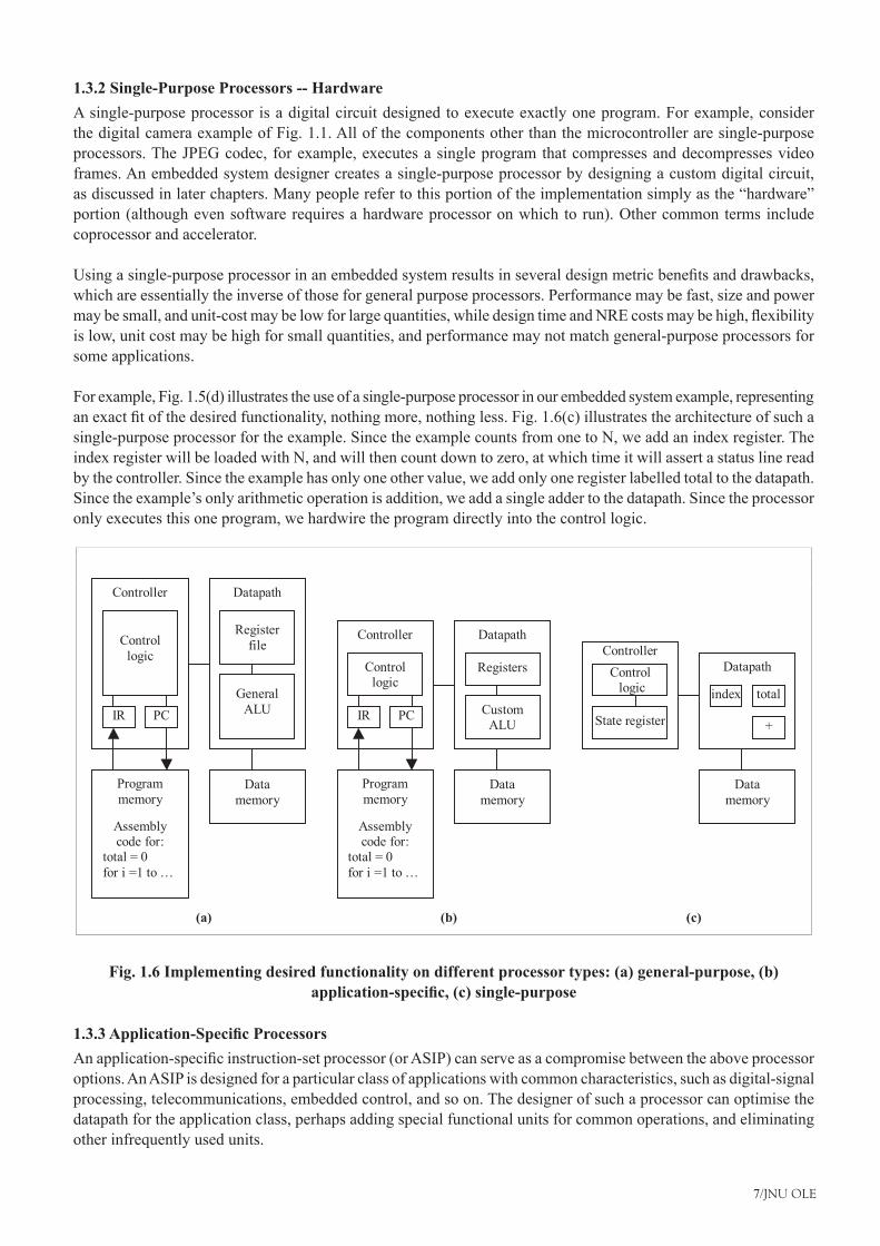
1.3.2 Single-Purpose Processors -- HardwareA single-purpose processor is a digital circuit designed to execute exactly one program. For example, consider the digital camera example of Fig. 1.1. All of the components other than the microcontroller are single-purpose processors. The JPEG codec, for example, executes a single program that compresses and decompresses video frames. An embedded system designer creates a single-purpose processor by designing a custom digital circuit, as discussed in later chapters. Many people refer to this portion of the implementation simply as the “hardware” portion (although even software requires a hardware processor on which to run). Other common terms include coprocessor and accelerator.

Usingasingle-purposeprocessorinanembeddedsystemresultsinseveraldesignmetricbenefitsanddrawbacks,which are essentially the inverse of those for general purpose processors. Performance may be fast, size and power maybesmall,andunit-costmaybelowforlargequantities,whiledesigntimeandNREcostsmaybehigh,flexibilityis low, unit cost may be high for small quantities, and performance may not match general-purpose processors for some applications.

For example, Fig. 1.5(d) illustrates the use of a single-purpose processor in our embedded system example, representing anexactfitofthedesiredfunctionality,nothingmore,nothingless.Fig.1.6(c)illustratesthearchitectureofsuchasingle-purpose processor for the example. Since the example counts from one to N, we add an index register. The index register will be loaded with N, and will then count down to zero, at which time it will assert a status line read by the controller. Since the example has only one other value, we add only one register labelled total to the datapath. Since the example’s only arithmetic operation is addition, we add a single adder to the datapath. Since the processor only executes this one program, we hardwire the program directly into the control logic.

Registerfile

GeneralALU

DatapathController

Programmemory

Assemblycode for:

total = 0for i =1 to …

IR PC

Controllogic

Registers

CustomALU

DatapathController

Programmemory

Assemblycode for:

total = 0for i =1 to …

Controllogic

DatapathController

Controllogic

State register

Datamemory

Datamemory

Datamemory

index total

+IR PC

(a) (b) (c)

Fig. 1.6 Implementing desired functionality on different processor types: (a) general-purpose, (b) application-specific, (c) single-purpose

1.3.3 Application-Specific ProcessorsAnapplication-specificinstruction-setprocessor(orASIP)canserveasacompromisebetweentheaboveprocessoroptions. An ASIP is designed for a particular class of applications with common characteristics, such as digital-signal processing, telecommunications, embedded control, and so on. The designer of such a processor can optimise the datapath for the application class, perhaps adding special functional units for common operations, and eliminating other infrequently used units.


8/JNU OLE

UsinganASIPinanembeddedsystemcanprovidethebenefitofflexibilitywhilestillachievinggoodperformance,power and size. However, such processors can require large NRE cost to build the processor itself, and to build a compiler, if these items don’t already exist. Much research currently focuses on automatically generating such processors and associated retargetable compilers. Due to the lack of retargetable compilers that can exploit the unique features of a particular ASIP, designers using ASIPs often write much of the software in assembly language.

Digital-signal processors (DSPs) are a common class of ASIP, so demand special mention. A DSP is a processor designed to perform common operations on digital signals, which are the digital encodings of analog signals like videoandaudio.Theseoperationscarryoutcommonsignalprocessingtaskslikesignalfiltering,transformation,or combination. Such operations are usually math-intensive, including operations like multiply and add or shift and add. To support such operations, a DSP may have special purpose datapath components such a multiply-accumulate unit, which can perform a computation like T = T + M[i]*k using only one instruction. Because DSP programs often manipulate large arrays of data, a DSP may also include special hardware to fetch sequential data memory locations in parallel with other operations, to further speed execution.

Fig. 1.5(c) illustrates the use of an ASIP for our example; while partially customised to the desired functionality, thereissomeinefficiencysincetheprocessoralsocontainsfeaturestosupportreprogramming.Fig.1.6(b)showsthe general architecture of an ASIP for the example. The datapath may be customised for the example. It may have an auto-incrementing register, a path that allows the add of a register plus a memory location in one instruction, fewer registers, and a simpler controller.

source drainchanneloxidegate

Silicon substrate

IC package IC

Fig. 1.7 A simplified CMOS transistor

1.4 IC TechnologyEvery processor must eventually be implemented on an IC. IC technology involves the manner in which we map a digital (gate-level) implementation onto an IC. An IC (Integrated Circuit), often called a “chip,” is a semiconductor device consisting of a set of connected transistors and other devices. A number of different processes exist to build semiconductors, the most popular of which is CMOS (Complementary Metal Oxide Semiconductor). The IC technologies differ by how customised the IC is for a particular implementation. For lack of a better term, we call these technologies “IC technologies.” IC technology is independent from processor technology; any type of processor can be mapped to any type of IC technology, as illustrated in Fig. 1.8.

TounderstandthedifferencesamongICtechnologies,wemustfirstrecognisethatsemiconductorsconsistofnumerouslayers. The bottom layers form the transistors. The middle layers form logic gates. The top layers connect these gates with wires. One way to create these layers is by depositing photo-sensitive chemicals on the chip surface and then shining light through masks to change regions of the chemicals. Thus, the task of building the layers is actually one of designing appropriate masks. A set of masks is often called a layout. The narrowest line that we can create on a chip is called the feature size, which today is well below one micrometer (sub-micron). For each IC technology, all layers must eventually be built to get a working IC; the question is who builds each layer and when.

9/JNU OLE

1.4.1 Full-Custom/VLSIIn a full-custom IC technology, we optimise all layers for our particular embedded system’s digital implementation. Such optimisation includes placing the transistors to minimise interconnection lengths, sizing the transistors to optimise signal transmissions and routing wires among the transistors. Once we complete all the masks, we send themaskspecificationstoafabricationplantthatbuildstheactualICs.Full-customICdesign,oftenreferredtoasVLSI (Very Large Scale Integration) design, has very high NRE cost and long turnaround times (typically months) before the IC becomes available, but can yield excellent performance with small size and power. It is usually used only in high-volume or extremely performance-critical applications.

1.4.2 Semi-Custom ASIC (gate array and standard cell)InanASIC(Application-SpecificIC)technology,thelowerlayersarefullyorpartiallybuilt,leavingustofinishthe upper layers. In a gate array technology, the masks for the transistor and gate levels are already built (i.e., the IC already consists of arrays of gates). The remaining task is to connect these gates to achieve our particular implementation. In a standard cell technology, logic-level cells (such as an AND gate or an AND-OR-INVERT combination) have their mask portions pre-designed, usually by hand. Thus, the remaining task is to arrange these portions into complete masks for the gate level, and then to connect the cells. ASICs are by far the most popular IC technology, as they provide for good performance and size, with much less NRE cost than full-custom IC’s.

General-purpose

processorASIP

Single-purpose

processor

Semi-customPLD Full-custom

Generalproviding improved:

Customized,providing improved:

Power efficiencyPerformance

SizeCost (high volume)

FlexibilityNRE cost

Time to prototypeTime to market

Cost (low volume)

Fig. 1.8 The independence of processor and IC technologies

1.4.3 PLDIn a PLD (Programmable Logic Device) technology, all layers already exist, so we can purchase the actual IC. The layers implement a programmable circuit, where programming has a lower-level meaning than a software program. The programming that takes place may consist of creating or destroying connections between wires that connect gates, either by blowing a fuse, or setting a bit in a programmable switch. Small devices, called programmers, connected to a desktop computer can typically perform such programming. We can divide PLD’s into two types, simple and complex. One type of simple PLD is a PLA (Programmable Logic Array), which consists of a programmable array of AND gates and a programmable array of OR gates. Another type is a PAL (Programmable Array Logic), which uses just one programmable array to reduce the number of expensive programmable components. One type of complex PLD, growing very rapidly in popularity over the past decade, is the FPGA (Field Programmable Gate Array), which offers more general connectivity among blocks of logic, rather than just arrays of logic as with PLAs and PALs, and is thus able to implement far more complex designs. PLDs offer very low NRE cost and almost instant IC availability. However, they are typically bigger than ASICs, may have higher unit cost, may consume more power, and may be slower (especially FPGAs). They still provide reasonable performance, though, so are especially well suited to rapid prototyping.


10/JNU OLE

As mentioned earlier and illustrated in Fig. 1.8, the choice of an IC technology is independent of processor types. For example, a general-purpose processor can be implemented on a PLD, semi-custom, or full-custom IC. In fact, acompanymarketingacommercialgeneral-purposeprocessormightfirstmarketasemi-customimplementationtoreachthemarketearly,andthenlaterintroduceafull-customimplementation.Theymightalsofirstmaptheprocessor to an older but more reliable technology, like 0.2 micron, and then later map it to a newer technology, like 0.08 micron. These two evolutions of mappings to a large extent explain why a processor’s clock speed improves on the market over time.

Furthermore, we often implement multiple processors of different types on the same IC. Fig. 1.1 was an example of just such a situation – the digital camera included a microcontroller (general-purpose processor) plus numerous single-purpose processors on the same IC.

Libraries/IP: Incorporatespre-designedimplementation fromlower abstraction levelinto higher level.

Systemspecification

Behavioralspecification

RTspecification

Logicspecification

To final implementation

Compilation/Synthesis:Automates explorationand insertion ofimplementation detailsfor lower level.

Test/Verification: Ensurescorrect functionality ateach level, thus reducingcostly iterations betweenlevels.

Compilation/Synthesis

Libraries/IP

Test/Verficiation

Systemsynthesis

Behaviorsynthesis

RTsynthesis

Logicsynthesis

Hw/Sw/OS

Cores

RTcomponents

Gates/Cells

Model simulat./checkers

Hw-swcosimulators

HDL simulators

Gatesimulators

Fig. 1.9 Ideal top-down design process and productivity improvers

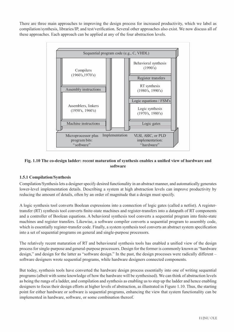
1.5 Design TechnologyDesign technology involves the manner in which we convert our concept of desired system functionality into an implementation. We must not only design the implementation to optimise design metrics, but we must do so quickly. As described earlier, the designer must be able to produce larger numbers of transistors every year, to keep pace with IC technology. Hence, improving design technology to enhance productivity has been a focus of the software and hardware design communities for decades.

Tounderstandhowtoimprovethedesignprocess,wemustfirstunderstandthedesignprocessitself.Variationsofatop-down design process have become popular in the past decade, an ideal form of which is illustrated in Figure 1.9. Thedesignerrefinesthesystemthroughseveralabstractionlevels.Atthesystemlevel,thedesignerdescribesthedesired functionality in some language, often a natural language like English, but preferably an executable language likeC;weshallcallthisthesystemspecification.Thedesignerrefinesthisspecificationbydistributingportionsofitamongchosenprocessors(generalorsinglepurpose),yieldingbehaviouralspecificationsforeachprocessor.Thedesignerrefinesthesespecificationsintoregister-transfer(RT)specificationsbyconvertingbehaviorongeneral-purpose processors to assembly code, and by converting behavior on single-purpose processors to a connection of register-transfercomponentsandstatemachines.Thedesignerthenrefinestheregister-transfer-levelspecificationofasingle-purposeprocessorintoalogicspecificationconsistingofBooleanequations.

Finally,thedesignerrefinestheremainingspecificationsintoanimplementation,consistingofmachinecodeforgeneral-purpose processors, and a gate-level netlist for single-purpose processors.

11/JNU OLE

There are three main approaches to improving the design process for increased productivity, which we label as compilation/synthesis,libraries/IP,andtest/verification.Severalotherapproachesalsoexist.Wenowdiscussallofthese approaches. Each approach can be applied at any of the four abstraction levels.

Implementation

Assembly instructions

Machine instructions Logic gates

Logic equations / FSM's

Register transfers

Sequential program code (e.g., C, VHDL)

Compilers(1960’s,1970’s)

Assemblers, linkers(1950’s, 1960’s)

Behavioral synthesis(1990’s)

RT synthesis(1980’s, 1990’s)

Logic synthesis(1970’s, 1980’s)

Microprocessor plusprogram bits:

“software”

VLSI, ASIC, or PLDimplementation:

“hardware”

Fig. 1.10 The co-design ladder: recent maturation of synthesis enables a unified view of hardware and software

1.5.1 Compilation/SynthesisCompilation/Synthesis lets a designer specify desired functionality in an abstract manner, and automatically generates lower-level implementation details. Describing a system at high abstraction levels can improve productivity by reducing the amount of details, often by an order of magnitude that a design must specify.

A logic synthesis tool converts Boolean expressions into a connection of logic gates (called a netlist). A register-transfer(RT)synthesistoolconvertsfinite-statemachinesandregister-transfersintoadatapathofRTcomponentsandacontrollerofBooleanequations.Abehavioralsynthesistoolconvertsasequentialprogramintofinite-statemachines and register transfers. Likewise, a software compiler converts a sequential program to assembly code, whichisessentiallyregister-transfercode.Finally,asystemsynthesistoolconvertsanabstractsystemspecificationinto a set of sequential programs on general and single-purpose processors.

TherelativelyrecentmaturationofRTandbehaviouralsynthesistoolshasenabledaunifiedviewofthedesignprocess for single-purpose and general-purpose processors. Design for the former is commonly known as “hardware design,” and design for the latter as “software design.” In the past, the design processes were radically different – software designers wrote sequential programs, while hardware designers connected components.

But today, synthesis tools have converted the hardware design process essentially into one of writing sequential programs (albeit with some knowledge of how the hardware will be synthesised). We can think of abstraction levels as being the rungs of a ladder, and compilation and synthesis as enabling us to step up the ladder and hence enabling designers to focus their design efforts at higher levels of abstraction, as illustrated in Figure 1.10. Thus, the starting point for either hardware or software is sequential programs, enhancing the view that system functionality can be implemented in hardware, software, or some combination thereof.


12/JNU OLE

The choice of hardware versus software for a particular function is simply a trade-off among various design metrics, likeperformance,power,size,NREcost,andespeciallyflexibility;thereisnofundamentaldifferencebetweenwhatthetwocanimplement.Hardware/softwareco-designisthefieldthatemphasisesthisunifiedview,anddevelopssynthesis tools and simulators that enable the co-development of systems using both hardware and software.

1.5.2 Libraries/IPLibraries involve re-use of pre-existing implementations. Using libraries of existing implementations can improve productivityifthetimeittakestofind,acquire,integrateandtestalibraryitemislessthanthatofdesigningtheitem oneself. A logic-level library may consist of layouts for gates and cells. An RT-level library may consist of layouts for RT components, like registers, multiplexors, decoders, and functional units. A behavioural-level library may consist of commonly used components, such as compression components, bus interfaces, display controllers, and even general purpose processors. The advent of system-level integration has caused a great change in this level of library. Rather than these components being IC’s, they now must also be available in a form, called cores that we can implement on just one portion of an IC. This change from behavioural-level libraries of IC’s to libraries of cores has prompted use of the term Intellectual Property (IP), to emphasise the fact that cores exist in a “soft” form that must be protected from copying. Finally, a system-level library might consist of complete systems solving particular problems, such as an interconnection of processors with accompanying operating systems and programs to implement an interface to the Internet over an Ethernet network.

1.5.3 Test/VerificationTest/Verification involves ensuring that functionality is correct. Such assurance can prevent time-consumingdebugging at low abstraction levels and iterating back to high abstraction levels. Simulation is the most common methodoftestingforcorrectfunctionality,althoughmoreformalverificationtechniquesaregrowinginpopularity.At the logic level, gate level simulators provide output signal timing waveforms given input signal waveforms.

Likewise, general-purpose processor simulators execute machine code. At the RT-level, hardware description language (HDL) simulators execute RT-level descriptions and provide output waveforms given input waveforms. At the behavioural level, HDL simulators simulate sequential programs, and co-simulators connect HDL and general purposeprocessorsimulatorstoenablehardware/softwareco-verification.Atthesystemlevel,amodelsimulatorsimulates the initial system specification using an abstract computationmodel, independent of any processortechnology, toverifycorrectnessandcompletenessof thespecification.Modelcheckerscanalsoverifycertainpropertiesofthespecification,suchasensuringthatcertainsimultaneousconditionsneveroccur,orthatthesystemdoes not deadlock.

1.5.4 Other Productivity ImproversThere are numerous additional approaches to improving designer productivity. Standards focus on developing well-definedmethodsforspecification,synthesisandlibraries.Suchstandardscanreducetheproblemsthatarisewhena designer uses multiple tools, or retrieves or provides design information from or to other designers. Common standards include language standards, synthesis standards and library standards. Languages focus on capturing desired functionality with minimum designer effort.

For example, the sequential programming language of C is giving way to the object oriented language of C++, which in turn has given some ground to Java. As another example, state-machine languages permit direct capture of functionality as a set of states and transitions, which can then be translated to other languages like C.

Frameworks provide a software environment for the application of numerous tools throughout the design process and management of versions of implementations. For example, a framework might generate the UNIX directories needed for various simulators and synthesis tools, supporting application of those tools through menu selections in a single graphical user interface.

13/JNU OLE

SummaryAn embedded system is nearly any computing system other than a desktop, laptop, or mainframe computer.•Single-functioned embedded system usually executes only one program, repeatedly•Tightly constrained embedded systems have constraints on design metrics, but those on embedded systems can •be especially tight.Many embedded systems must continually react to changes in the system’s environment, and must compute •certain results in real time without delay.A single-purpose processor is a digital circuit designed to execute exactly one program. •Digital-signal processors (DSPs) are a common class of ASIP, so demand special mention. A DSP is a processor •designed to perform common operations on digital signals, which are the digital encodings of analog signals like video and audio. In a PLD (Programmable Logic Device) technology, all layers already exist, so we can purchase the actual •IC.Design technology involves the manner in which we convert our concept of desired system functionality into •an implementation.Compilation/Synthesis lets a designer specify desired functionality in an abstract manner, and automatically •generates lower-level implementation details.

ReferencesChapter 1 Introduction• , [pdf] Available at: <http://www.cs.ucr.edu/~vahid/courses/122a_f99/ch1.pdf> [Accessed 4 July 2012].Prof. Edwards, S. A., • Embedded Systems, [pdf] Available at: <http://www.cs.columbia.edu/~sedwards/classes/2005/4840/embedded-systems.pdf> [Accessed 4 July 2012].Kamal, R., 2008. • Embedded Systems, 2nd ed., Tata McGraw-Hill Education.Barrett, • Embedded Systems, Pearson Education India.2008, • Lecture -1 Embedded Systems: Introduction, [Video Online] Available at: <http://www.youtube.com/watch?v=y9RAhEfLfJs> [Accessed 4 July 2012].2010, • Introduction to embedded systems, [Video Online] Available at: <http://www.youtube.com/watch?v=Uzm2uUuAYlE> [Accessed 4 July 2012].

Recommended ReadingPeckol, J. K., 2007. • Embedded Systems: A Contemporary Design Tool, 1st ed., Wiley.Barr, M. & Massa, A., 2006. • Programming Embedded Systems: With C and GNU Development Tools, 2nd ed.,O’Reilly Media.Lipiansky, E., 2011. • Embedded Systems Hardware for Software Engineers, 1st ed., McGraw-Hill Professional.


14/JNU OLE

Self AssessmentWhich of the following statements is true?1.

Test/Verificationinvolvesensuringthatfunctionalityiscorrect.a. Test/Verificationinvolvesensuringthatcompatibilityiscorrect.b. Evaluation involves ensuring that functionality is correct.c. Test/Verificationinvolvesensuringthatprogrammingiscorrect.d.

________ involve re-use of pre-existing implementations.2. Databasea. Librariesb. Expressionsc. Applicationsd.

Which of the following library may consist of layouts for gates and cells?3. Design-levela. Logic-levelb. RT-levelc. Application-leveld.

An ______________ library may consist of layouts for RT components, like registers, multiplexors, decoders, 4. and functional units.

Design-levela. RS-levelb. Logic-levelc. RT-leveld.

A logic synthesis tool converts Boolean expressions into a connection of_________.5. logic gatesa. IC’sb. chipsc. ASICd.

_____________ technology involves the manner in which we convert our concept of desired system functionality 6. into an implementation.

ICa. Designb. DSPc. Computerd.

Inan____________technology, the lower layersarefullyorpartiallybuilt, leavingus tofinish theupper7. layers.

ASICa. DSPb. ICc. ASIPd.

15/JNU OLE

A _____________ is a processor designed to perform common operations on digital signals, which are the 8. digital encodings of analog signals like video and audio.

DSPa. ASICb. PLDc. VPLDd.

In a _____________ technology, all layers already exist, so we can purchase the actual IC.9. VPLDa. PLDb. DSPc. ASICd.

In a full-custom ____________ technology, we optimise all layers for our particular embedded system’s digital 10. implementation.

ICa. PLDb. DSPc. ASICd.


16/JNU OLE

Chapter II

Overview of Microcontrollers

Aim


introduce microcontrollers•

compare microprocessors and microcontrollers•

enlist the types of microcontrollers •

Objectives


explain Von-Neumann architecture•

explicate Harvard architecture•

elucidate CISC architecture microcontrollers•

Learning outcome


understand RISC architecture microcontrollers•

identify SISC •

enlist the microcontroller app• lications

17/JNU OLE

2.1 IntroductionMicrocontrollers have only been with us for a few decades but their impact (direct or indirect) on our lives is profound. Usually these are supposed to be just data processors performing exhaustive numeric operations. But their presence is unnoticed at most of the places like

At supermarkets in Cash Registers, Weighing Scales, and so on•At home in Ovens, Washing Machines, Alarm Clocks,and so on.•At play in Toys, VCRs, Stereo Equipment, and so on.•AtofficeinTypewriters,Photocopiers,Elevators,andsoon.•In industry in Industrial Automation, safety systems, and so on.•OnroadsinCars,TrafficSignals,andsoon.•

What inside them makes these machines smart? The answer is microcontroller. Creating applications for the microcontrollers is different than any other development job in electronics and computing. Before selecting a particular device for an application, it is important to understand what the different options and features are and what they can mean with regard to developing the application.

The purpose of this chapter is to introduce the concept of microcontrollers, how it differs from microprocessors and different type of commercial microcontrollers available as well as their applications.

2.2 Embedded ControllerSimplyanembeddedcontrollerisacontrollerthatisembeddedinagreatersystem.Onecandefineanembeddedcontroller as a controller (or computer) that is embedded into some device for some purpose other than to provide generalpurposecomputing.Isanembeddedcontrolleristhesameasamicrocontroller?Theanswerisdefinitelyno. One can state devices such as 68000, 32032, x86, Z80, and so on that are used as embedded controllers but they aren’t microcontrollers.

We might be correct by stating that an embedded controller controls something (for example controlling a device such as a microwave oven, car braking system or a cruise missile). An embedded controller may also embed the on-chip resources like a microcontroller. Microcontrollers and microprocessors are widely used in embedded systems. However, microcontrollers are preferred over microprocessors for embedded systems due to low power consumption.

2.3 Microcontrollers and MicroprocessorsA controller is used to control some process. At one time, controllers were built exclusively from logic components, andwereusuallylarge,heavyboxes.Lateron,microprocessorswereusedandtheentirecontrollercouldfitonasmallcircuitboard.Thisisstillcommon–onecanfindmanycontrollerspoweredbyoneofthemanycommonmicroprocessors (including Zilog Z80, Intel 8088, Motorola 6809, and others).

As the process of miniaturisation continued, all of the components needed for a controller were built right onto one chip. A one chip computer or microcontroller was born. A CPU built into a single VLSI chip is called microprocessor. ThesimplifiedblockdiagramoftheCPUisshowninthefigurebelow.Itcontainsarithmeticandlogicunit(ALU),Instruction decode and control unit, Instruction register, Program counter (PC), clock circuit (internal or external), reset circuit (internal or external) and registers. For example,

Intel 8085 is 8-bit microprocessor and Intel 8086/8088 is 16-bit microprocessor. Microprocessor is general-purpose digital computer central processing unit (CPU). The microprocessor is general-purpose device and additional external circuitry is added to make it microcomputer.


18/JNU OLE

Holds the memoryaddress of the nextinstruction to beexecuted.

Temporary storageof information.

Holds the binary codefor each instruction asit is executed

Determines theoperation to performand sets in motion the necessary actions toperform it.

Performs arithmeticand logic operations

InstructionReg ister (IR)

ProgramCounter (PC)

InstructionDecode &

Control Unit

Arithmetic &Lo g ic Unit

(ALU)

Registers

Fig. 2.1 General block diagram of CPU (Microprocessor)

A digital computer having microprocessor as the CPU along with I/O devices and memory is known as microcomputer. Theblockdiagraminthefigureaboveshowsamicrocomputer.

ROMRAMInterfaceCircuitry

PeripheralDevices

CPU

Address Bus

Data Bus

Control Bus

Fig. 2.2 Microcomputer block diagram

A microcontroller is a highly integrated chip, which includes on single chip, all or most of the parts needed for a controller. The microcontroller typically includes: CPU (Central Processing Unit), RAM (Random Access Memory), EPROM/PROM/ROM (Erasable Programmable Read Only Memory), I/O (input/output) – serial and parallel, timers, interrupt controller. For example, Intel 8051 is 8-bit microcontroller and Intel 8096 is 16-bit microcontroller.

19/JNU OLE

I/OPorts

Interruptcircuits

ClockCircuit

Program Counter

ALU

InternalRAM

Register(S)

ACC

SPTimer/Counter

InternalRom

Fig. 2.3 A block diagram of a microcontroller

Byonlyincludingthefeaturesspecifictothetask(control),costisrelativelylow.Atypicalmicrocontrollerhasbitmanipulationinstructions,easyanddirectaccesstoI/O(input/output),andquickandefficientinterruptprocessing.Figure above shows the block diagram of a typical microcontroller.

Comparing Microprocessors and MicrocontrollersMicroprocessor is a single chip CPU, microcontroller contains, a CPU and much of the remaining circuitry of •a complete microcomputer system in a single chip.Microcontroller includes RAM, ROM, serial and parallel interface, timer, interrupt schedule circuitry (in addition •to CPU) in a single chip.

RAM is smaller than that of even an ordinary microcomputer, but enough for its applications. �Interrupt system is an important feature, as microcontrollers have to respond to control oriented devices in �real time. For example, opening of microwave oven’s door cause an interrupt to stop the operation. (Most microprocessors can also implement powerful interrupt schemes, but external components are usually needed).

Microprocessors are most commonly used as the CPU in microcomputer systems. Microcontrollers are used •in small, minimum component designs performing control-oriented activities.Microprocessor instruction sets are processing intensive, implying powerful addressing modes with instructions •catering to large volumes of data. Their instructions operate on nibbles, bytes, etc. Microcontrollers have instruction sets catering to the control of inputs and outputs. Their instructions operate also on a single bit. For example, a motor may be turned ON and OFF by a 1-bit output port.

Beforegoing in todetailsofmicrocontrollers itwillbebeneficial togo throughcommonand frequentlyusedterminology encountered in the description of microcontrollers.


20/JNU OLE

2.3.1 Central Processing Unit (CPU)CPU is the brain of the computer system, administers all activity in the system and performs all operations on data. It continuously performs two operations: fetching and executing instructions. It understands and executes instructions based on a set of binary codes called the instruction set.

Machine CycleTo execute an instruction–the processor must:

Fetch the instruction from memory•Decode the instruction•Execute the instruction•Store the result back in the memory. These four steps refer to Machine Cycle.•

Generally one machine cycle = X clock cycles (Xdepends on the particular instruction being executed). Shorter the clock cycle, lesser the time it takes to complete one machine cycle, so instructions are executed faster. Hence, faster the processor.

2.3.2 Fetching and Executing an InstructionFetching involves the following steps:

Contents of PC are placed on address bus.•READ signal is activated.•Data (instruction opcode) are read from RAM and placed on data bus.•Opcode is latched into the CPU’s internal instruction register.•PC is incremented to prepare for the next fetch from memory.•

While execution involves decoding the opcode and generating control signals to gate internal registers in and out oftheALUandtosignaltheALUtoperformthespecifiedoperation.

2.3.3 The Buses: Address, Data, and ControlA BUS is a collection of wires carrying information with a common purpose. For each read or write operation, the CPUspecifiesthelocationofthedataorinstructionbyplacinganaddressontheaddressbusthenactivatesasignalon the control bus indicating whether the operation is read or write.

READoperationsretrieveabyteofdatafrommemoryatthelocationspecifiedandplaceitonthedatabus.•CPU reads the data and places it in one of its internal registers.WRITEoperationsputdatafromCPUonthedatabusandstoreitinthelocationspecified.•ADDRESSBUScarriestheaddressofaspecifiedlocation.Fornaddresslines,2nlocationscanbeaccessed.•For example, A 16-bit address bus can access 216 = 65,536 locations or 64K locations (210 = 1024 = 1K, 26 = 64).DATA BUS carries information between the CPU and memory or between the CPU and I/O devices.•CONTROL BUS carries control signals supplied by the CPU to synchronise the movement of information on •the address and data bus.

2.3.4 Control/Monitor (Input/output) DevicesControl devices are outputs, or actuators, that can affect the world around them when supplied with a voltage or current.

Monitoring devices are inputs, or sensors, that are stimulated by temperature, pressure, light, motion, etc. and convert this to voltage or current read by the computer. Note: The interface circuitry converts the voltage or current to binary data, or vice versa.

21/JNU OLE

2.4 Types of MicrocontrollersMicrocontrollerscanbeclassifiedonthebasisofinternalbuswidth,architecture,memoryandinstructionset.Fig.2.4 shows the various types of microcontrollers.

2.4.1 The 8,16 and 32-Bit MicrocontrollersThe 8-Bit MicrocontrollerWhen the ALU performs arithmetic and logical operations on a byte (8-bits) at an instruction, the microcontroller is an 8-bit microcontroller. The internal bus width of 8-bit microcontroller is of 8-bit. Examples of 8-bit microcontrollers are Intel 8051 family and Motorola MC68HC11 family.

The 16-Bit MicrocontrollerWhen the ALU performs arithmetic and logical operations on a word (16-bits) at an instruction, the microcontroller is a 16-bit microcontroller. The internal bus width of 16-bit microcontroller is of 16-bit. Examples of 16-bit microcontrollers are Intel 8096 family and Motorola MC68HC12 and MC68332 families. The performance and computing capability of 16 bit microcontrollers are enhanced with greater precision as compared to the 8-bit microcontrollers.

The 32-Bit MicrocontrollerWhen the ALU performs arithmetic and logical operations on a double word (32- bits) at an instruction, the microcontroller is a 32-bit microcontroller. The internal bus width of 32-bit microcontroller is of 32-bit. Examples of 32-bit microcontrollers are Intel 80960 family and Motorola M683xx and Intel/Atmel 251 family. The performance and computing capability of 32 bit microcontrollers are enhanced with greater precision as compared to the 16-bit microcontrollers.

Microcontrollers

Bits Memory/devices Instruction set Memory architecture

4 8 16 32 Embedded External CISC RISC Princeton Harvard

Family

8051 Motorola PIC ARM othersNationalTexas

Intel Atmel Dallas Phillips Siemens

Fig. 2.4 Types of Microcontrollers


22/JNU OLE

2.5 Embedded and External Memory MicrocontrollersEmbedded and external memory microcontrollers are explained below:

2.5.1 Embedded MicrocontrollersWhen an embedded system has a microcontroller unit that has all the functional blocks (including program as well as data memory) available on a chip is called an embedded microcontroller. For example, 8051 having Program & Data Memory, I/O Ports, Serial Communication, Counters and Timers and Interrupt Control logic on the chip is an embedded microcontroller.

2.5.2 External Memory MicrocontrollersWhen an embedded system has a microcontroller unit that has not all the functional blocks available on a chip is called an external memory microcontroller. In external memory microcontroller, all or part of the memory units are externally interfaced using an interfacing circuit called the glue circuit. For example, 8031 has no program memory on the chip is an external memory microcontroller.

2.6 Microcontroller Architectural FeaturesThere are mainly two categories of processors, namely, Von-Neumann (or Princeton) architecture and Harvard Architecture. These two architectures differ in the way data and programs are stored and accessed.

2.6.1 Von-Neumann ArchitectureMicrocontrollers based on the Von-Neumann architecture have a single data bus that is used to fetch both instructions and data. Program instructions and data are stored in a common main memory. When such a controller addresses mainmemory,itfirstfetchesaninstruction,andthenitfetchesthedatatosupporttheinstruction.Thetwoseparatefetches slows up the controller’s operation. Fig.2.5 shows the Von-Neumann Architecture. The Von-Neumann architecture’smainadvantageisthatitsimplifiesthemicrocontrollerdesignbecauseonlyonememoryisaccessed.In microcontrollers, the contents of RAM can be used for data storage and program instruction storage. For example, the Motorola 68HC11 microcontroller Von- Neumann architecture.

Example: An Instruction “Read a byte from memory and stores it in the accumulator” as follows:Cycle 1:- Read instructionCycle 2:- Read data out of RAM and put into Accumulator

ProgramROM

VariableRAM

StackRAM

Instruction Decode

Processorand Built-inRegisters

MemoryInterfaceUnit

Data

Addr

Ctrl

Memory space

Fig. 2.5 Von-Neumann architecture block diagram

23/JNU OLE

2.6.2 Harvard ArchitectureMicrocontrollers based on the Harvard Architecture have separate data bus and an instruction bus. This allows execution to occur in parallel. As an instruction is being “pre-fetched”, the current instruction is executing on the data bus. Once the current instruction is complete, the next instruction is ready to go. This pre-fetch theoretically allows for much faster execution than Von-Neumann architecture, on the expense of complexity. Fig. 2.6 shows the Harvard Architecture. The Harvard Architecture executes instructions in fewer instruction cycles than the Von-Neumann architecture. For example, the Intel MCS-51 family of microcontrollers and PIC microcontrollers uses Harvard Architecture.

The same instruction (as shown under Von-Neumann architecture) would be executed as follows:Cycle 1: - Complete previous instructionRead the “Move Data to Accumulator” instructionCycle 2: - Execute “Move Data to Accumulator” instructionRead next instruction

Hence each instruction is effectively executed in one instruction cycle.

Control space

ProgramROM

InstructionDecode

PC stack RegisterSpace

Ctrl

Addr

Data

Processor andRegister Interface

Ctrl

Addr

Data

Fig. 2.6 Harvard architecture block diagram

2.6.3 CISC (Complex Instruction Set Computer) Architecture MicrocontrollersAlmost all of today’s microcontrollers are based on the CISC (Complex Instruction Set Computer) concept. When a microcontroller has an instruction set that supports many addressing modes for the arithmetic and logical instructions, data transfer and memory accesses instructions, the microcontroller is said to be of CISC architecture.

The typical CISC microcontroller has well over 80 instructions, many of them very powerful and much specialised forspecificcontroltasks.Itisquitecommonfortheinstructionstoallbehavequitedifferently.Somemightonlyoperate on certain address spaces or registers, and others might only recognise certain addressing modes.

The advantages of the CISC architecture are that many of the instructions are macro like, allowing the programmer to use one instruction in place of many simpler instructions. An example of CISC architecture microcontroller is Intel 8096 family.


24/JNU OLE

2.6.4 RISC (Reduced Instruction Set Computer) Architecture MicrocontrollersThe industry trend for microprocessor design is for Reduced Instruction Set Computers (RISC) designs. When a microcontroller has an instruction set that supports fewer addressing modes for the arithmetic and logical instructions andfordatatransferinstructions,themicrocontrollerissaidtobeofRISCarchitecture.ThebenefitsofRISCdesignsimplicity are a smaller chip, smaller pin count, and very low power consumption. Some of the typical features of RISC processor- Harvard architecture are:

Allows simultaneous access of program and data.•Overlapping of some operations for increased processing performance.•Instruction pipelining increases execution speed.•Orthogonal (symmetrical) instruction set for programming simplicity.•Allows each instruction to operate on any register or use any addressing mode.•

2.6.5 SISC (Specific Instruction Set Computer)Actually,amicrocontrollerisbydefinitionaReducedInstructionSetComputer.ItcouldreallybecalledaSpecificInstruction Set Computer (SISC). The basic idea behind the microcontroller was to limit the capabilities of the CPU itself,allowingacompletecomputer(memory,I/O,interrupts,etc)tofitonthesinglechip.Attheexpenseofthemore general purpose instructions that make the standard microprocessors (8088, 68000, 32032) so easy to use, theinstructionsetwasdesignedforthespecificpurposeofcontrol(powerfulbitmanipulation,easyandefficientI/O, and so on).

2.7 Microcontroller ApplicationsIn addition to control applications such as the home monitoring system, microcontrollers are frequently found in embedded applications.Among themanyuses that you canfindoneormoremicrocontrollers: automotiveapplications, appliances (microwave oven, refrigerators, television and VCRs, stereos), automobiles (engine control, diagnostics, climate control), environmental control (greenhouse, factory, home), instrumentation, aerospace, and thousands of other uses.

Microcontrollersareusedextensivelyinrobotics.Inthisapplication,manyspecifictasksmightbedistributedamonga large number of microcontrollers in one system. Communications between each microcontroller and a central, more powerful microcontroller (or microcomputer, or even large computer) would enable information to be processed by the central computer, or to be passed around to other microcontrollers in the system. A special application that microcontrollersarewellsuitedforisdatalogging.Bystickoneofthesechipsoutinthemiddleofacornfieldorup in a balloon, one can monitor and record environmental parameters (temperature, humidity, rain, etc). Small size, lowpowerconsumption,andflexibilitymakethesedevicesidealforunattendeddatamonitoringandrecording.

2.8 Commercial Microcontroller DevicesMicrocontrollers come in many varieties. Depending on the power and features that are needed, one might choose a 4 bit, 8 bit, 16 bit, or 32 bit microcontroller. In addition, some specialised versions are available which include featuresspecificforcommunications,keyboardhandling,signalprocessing,videoprocessing,andothertasks.Theexamples of different types of commercial microcontroller devices are given in the following tables:

25/JNU OLE

Model (Manufacturer)

I/O Pins RAM (bytes)

ROM(bytes)

Counters Extra Features

COP400 Family(National)

23 28 64 1K 1 Serial bit I/O

HMCS40(Hitachi)

TMS 1000(TexasInstruments

10

23

28

28

32

64

512

1K

-

-

10-bit ROMLED display

Model (Manufacturer)

I/O Pins RAM (bytes)

ROM(bytes)

Counters Extra Features

8048 (Intel) 27 40 64 1K 1 8k External memory

8051 (Intel) 32 40 128 4K 2 128k External memory Boolean processing serial port

COP800 Family 24 28 64 1K 1 Serial bit I/O, 8- channelA/D converter(National)

6805 (Motorola) 20 28 64 1K 1 PLL frequency synthesiser

68hc11(Motorola) 40 52 256 8K 2 A/D, PWM generator, pulse accumulator

TMS370 (Texas) 55 68 256 4K 2 watchdog timer, Instruments) Serial ports ,A/D (8 bit, 8 channel)

PIC (Micro Chip) 12 18 25 1K 0 small pin count, verylow power consumption

Table 2.1 Different types of commercial microcontroller devices


26/JNU OLE

SummaryA digital computer having microprocessor as the CPU along with I/O devices and memory is known as •microcomputer.A microcontroller is a highly integrated chip, which includes on single chip, all or most of the parts needed for •a controller.Microprocessors are most commonly used as the CPU in microcomputer systems.•Microcontrollers are used in small, minimum component designs performing control-oriented activities.•Microprocessor instruction sets are processing intensive, implying powerful addressing modes with instructions •catering to large volumes of data.CPU is the brain of the computer system, administers all activity in the system and performs all operations on •data.A BUS is a collection of wires carrying information with a common purpose.•Control devices are outputs, or actuators, that can affect the world around them when supplied with a voltage •or current.When the ALU performs arithmetic and logical operations on a byte (8-bits) at an instruction, the microcontroller •is an 8-bit microcontroller. When the ALU performs arithmetic and logical operations on a word (16-bits) at an instruction, the microcontroller •is a 16-bit microcontroller. When the ALU performs arithmetic and logical operations on a double word (32- bits) at an instruction, the •microcontroller is a 32-bit microcontroller.

References Introduction to Microcontrollers• , [pdf] Available at: <http://www.newagepublishers.com/samplechapter/001599.pdf> [Accessed 6 July 2012].Mackenzie, • The 8051 Microcontroller, 4th ed., Pearson Education India.Godse, D. A. & Godse, A. P. 2009. • Microcontrollers, Technical Publications.Calcutt,D., Cowan, F. & Parchizadeh, H., • 8051 Microcontrollers An Applications-Based Introduction,[pdf] Available at: <http://ee.sharif.edu/~sakhtar3/books/8051%20Microcontrollers%20An%20Applications%20Based%20Introduction.pdf> [Accessed 6 July 2012].2010, • Chapter 2: The 8051 Hardware Architecture, [Video Online] Available at: <http://www.youtube.com/watch?v=Biw5qk-5JIs> [Accessed 6 July 2012].2009, • Microcontroller Tutorial Part-1, [Video Online] Available at: <http://www.youtube.com/watch?v=rRrCpcLllOM> [Accessed 6 July 2012].

Recommended Reading Crisp, J., 2004. • Introduction to Microprocessors and Microcontrollers, 1st ed., Newnes.Rizvi, S. R., 2011. • 8051 Microcontrollers: An Application Based Introduction, CRC Press.Lipovski, G. J., 2004. • Introduction to Microcontrollers, Academic Press.

27/JNU OLE

Self Assessment______________ are outputs, or actuators, that can affect the world around them when supplied with a voltage 1. or current.

Control devicesa. Input devicesb. Output devicec. Input/output devicesd.

Which of the following is general-purpose digital computer central processing unit (CPU)?2. Microchipa. Microprocessorb. Microcontrollerc. Interprocessor d.

A ____________ is a highly integrated chip, which includes on single chip, all or most of the parts needed for 3. a controller.

Microcontrollera. Microchipb. Microprocessorc. Interprocessor d.

_____ system is an important feature, as microcontrollers have to respond to control oriented devices in real 4. time.

Analoga. Digitalb. Computerc. Interruptd.

A ______________ is a collection of wires carrying information with a common purpose.5. BUSa. MANb. WANc. LANd.

When an _______________ system has a microcontroller unit that has all the functional blocks (including 6. program as well as data memory) available on a chip is called an embedded microcontroller.

embeddeda. interruptb. BUSc. computerd.

When an embedded system has a microcontroller unit that has not all the functional blocks available on a chip 7. is called an ___________ memory microcontroller.

externala. internalb. digitalc. analogd.


28/JNU OLE

Microcontrollers based on the ____________ architecture have a single data bus that is used to fetch both 8. instructions and data.

Von-Neumanna. Harvardb. BUSc. ASIPd.

The_____________architecture’smainadvantageisthatitsimplifiesthemicrocontrollerdesignbecauseonly9. one memory is accessed.

Harvarda. BUSb. ASIPc. Von-Neumannd.

Microcontrollers based on the _____________ Architecture have separate data bus and an instruction bus.10. Harvarda. BUSb. ASIPc. Von-Neumannd.

29/JNU OLE

Chapter III

Embedded System Hardware

Aim


explain simplifieddesigninformationflow•

enlist the input devices•

explicate output devices•

Objectives


explain sensors•

explicate D/A convertors•

elucidate actuators•

Learning outcome


understand A/D convertors•

describe image sensors•

enlist the communi• cation requirements


30/JNU OLE

3.1 IntroductionIt is one of the characteristics of embedded systems that both hardware and software must be taken into account. The reuse of available hard- and software components are at the heart of the proposed platform-based design methodology.

Consistentwiththeneedtoconsideravailablehardwarecomponentsandwiththedesigninformationflowshowninfigurebelow,wearenowgoingtodescribesomeoftheessentialsofembeddedsystemhardware.

specification

standard software

realizationimplementation: hw/sw codesign

... ...... (from all phases)

validation; evaluation (performance, energy consumption, safety, ..)

(RTOS, ...) software

...

hardware

egdelwonk noitacilppa

Fig. 3.1 Simplified design information flow

Hardware for embedded systems is much less standardized than hardware for personal computers. Due to the huge variety of embedded system hardware, it is impossible to provide a comprehensive overview over all types of hardware components. Nevertheless, we will try to provide an overview over some of the essential components which can be found in most systems. In many of the embedded systems, especially in control systems, embedded hardware is used in a loop.

display

D/A converter

sensors

informationprocessing

A/D converter

environment actuators

Fig. 3.2 Hardware in the loop

In this loop, information about the physical environment is made available through sensors. Typically, sensors generate continuous sequences of analog values. In this book, we will restrict ourselves to information processing in digital computers processing discrete sequences of values. Appropriate conversions are performed by two kinds of circuits: sample-and-hold-circuits and analog-to-digital (A/D) converters. After this conversion, information can be processed digitally. Generated results can be displayed and also be used to control the physical environment through actuators. Since most actuators are analog actuators, conversion from digital to analog signals is also needed.

Thismodelisobviouslyappropriateforcontrolapplications.Forotherapplications,itcanbeemployedasafirstorder approximation. For example, in mobile phones, sensors correspond to the antenna and actuators correspond to the speakers. In the following, we will describe essential hardware components of embedded systems following the loop structure of Fig. 3.2.

31/JNU OLE

3.2 Input3.2.1 SensorsSensors can be designed for virtually every physical quantity. There are sensors for weight, velocity, acceleration, electrical current, voltage, temperatures, etc. A large amount of physical effects can be used for constructing sensors. Examplesincludethelawofinduction(generationofvoltagesinanelectricfield),orlight-electriceffects.Also,there are sensors for chemical substances.

In recent years, a huge amount of sensors has been designed and much of the progress in designing smart systems can be attributed to modern sensor technology. Hence, it is impossible to cover this subset of embedded hardware technology comprehensively and we can only give characteristic examples:

Acceleration sensorsFigure below shows a small sensor manufactured using micro system technology. The sensor contains a small mass in its centre. When accelerated, the mass will be displaced from its standard position, thereby changing the resistance of the tiny wires connected to the mass.

Fig. 3.3 Acceleration sensor

Rain sensorsIn order to remove distraction from drivers, some recent high end cars contain rain sensors. Using these, the speed of the wipers can be automatically adjusted to the amount of rain.

Image sensorsThere are essentially two kinds of image sensors: charge coupled devices (CCDs) and CMOS sensors. In both cases, arrays of light sensors are used. The architecture of CMOS sensor arrays is similar to that of standard memories: individual pixels can be randomly addressed and read out. CMOS sensors use standard CMOS technology for integrated circuits. Due to this, sensors and logic circuits can be integrated on the same chip. This allows some pre-processing to be done already on the sensor chip, leading to so-called smart sensors. CMOS sensors require only a single standard supply voltage and interfacing in general is easy.

Therefore, CMOS-based sensors can be cheap. In contrast, CCD technology is optimized for optical applications. InCCDtechnology,chargeshavetobetransferredfromonepixeltothenextuntiltheycanfinallybereadoutatanarray boundary. This sequential charge transfer also gave CCDs their name. Images generated with CCDs can be of higher quality than those generated using CMOS sensors, since they generate less noise. However, interfacing is more complex. As a result, CMOS sensors are appropriate for applications requiring low or medium costs and low or medium image quality. CCD sensors are more adequate for high quality, expensive image sensors (such as those found in video cameras and optical telescopes, for example).


32/JNU OLE

Bio-metrical sensorsDemands for higher security standards as well as the need to protect mobile and removable equipment have led to an increased interest in authentication. Due to the limitations of password based security (example, stolen and lost passwords), smartcards, bio-metrical sensors andbio-medical authentication receive significant attention.Bio-medical authentication tries to identify whether or not a certain person is actually the person she or he claims tobe.Methodsforbio-medicalauthenticationincludeirisscans,fingerprintsensorsandfacerecognition.Fingerprint sensors are typically fabricated using the same CMOS technology which is used for manufacturing integrated circuits.Possibleapplicationsincludenotebookswhichgrantaccessonlyiftheuser’sfingerprintsisrecognized.CCD and CMOS image sensors described above are used for face recognition. False accepts as well as false rejects are an inherent problem of bio-medical authentication. In contrast to password based authentication, exact matches are not possible.

3.2.2 Sample-and-Hold CircuitsAll known digital computers work in the discrete time domain. This means they can process discrete sequences of values. Hence, values in the continuous domain have to be converted to the discrete domain. This is the purpose of sample-and-hold circuits. Fig. 3.4 (left) shows a simple sample-and-hold circuit.

In essence, the circuit consists of a clocked transistor and a capacitor. The transistor operates like a switch. Each time the switch is closed by the clock signal, the capacitor is charged so that its voltage is practically the same as the incoming voltage Ve. After opening the switch again, this voltage will

VeV Vx e

Vx

t

U

Clock

Fig. 3.4 Sample-and-hold-circuit

remain essentially unchanged until the switch is closed again. Each of the values stored on the capacitor can be considered as an element of a discrete sequence of values Vx, generated from a continuous sequence Ve.

An ideal sample-and-hold circuit would be able to change the voltage at the capacitor in an arbitrarily short amount of time. This way, the input voltage at a particular instance in time could be transferred to the capacitor and each element in the discrete sequence would correspond to the input voltage at a particular point in time. In practice, however, the transistor has to be kept closed for a short time window in order to really charge or discharge the capacitor. The voltage stored on the capacitor will then correspond to a voltage averaged over that short time window

3.2.3 A/D-ConvertersSince we are restricting ourselves to digital computers, we will also have to work with discrete values representing our input signals. The conversion from analog to digital values is done by analog-to-digital (A/D) converters. There is a large range of A/D converters with varying speed/precision characteristics. Here are the types of A/D-converters.

Flash A/D converterThis type of A/D converters uses a large number of comparators. Each comparator has two inputs, denoted as + and -. If the voltage at input + exceeds that at input -, the output corresponds to a logical ’1’ and it corresponds to a logical ’0’ otherwise1.

In the A/D-converter, all - inputs are connected to a voltage divider. Now, if input voltage Vx exceeds constant voltage Vref,thecomparatoratthetopoffigurebelowwillgeneratea’1’.Theencoderattheoutputofthecomparatorswilltrytoidentifythemostsignificant’1’andwillencodethecaseofVx>Vrefasthelargestoutputvalue.

33/JNU OLE

xV

+

+

Vref

_4

Vref3

R

R

R

R

_4 ref

_4 ref2

1

+

+

gnidocnE outputs

Digital

Comparators

V

V

Fig. 3.5 Flash A/D converter

NowifinputvoltageVxislessthanVref,butstilllargerthan¾Vref,thecomparatoratthetopoffig.3.5willgenerate a ’0’, while the next comparator will still signal a ’1’. The encoder will encode this as the second-largest value.

Similar arguments hold for cases 2/4 Vref < Vx < 3/4Vref, ¼ Vref < Vx < 2/4 Vref , and 0 < Vx < ¼ Vref , which will be encoded as the third-largest, fourth largest and smallest value, respectively.

The circuit can convert positive analog input voltages into digital values. Converting both positive and negative voltages requires some extensions.

The key advantage of the circuit is its speed. It does not need any clock. The delay between the input and the output is very small and the circuit can be used easily, for example, for high-speed video applications. The disadvantage isitshardwarecomplexity:weneedn−1comparatorsinordertodistinguishbetweennvalues.ImagineusingthiscircuitingeneratingdigitalaudiosignalsforCDrecorders.Wewouldneed216−1comparators.

Successive approximationDistinguishing between a large numbers of digital values is possible with A/D converters using successive approximation.

Thecircuitisshowninthefigurebelow.

Thekeyideaofthiscircuitistousebinarysearch.Initially,thesignificantoutputbitofthesuccessiveapproximationregister is set to ’1’, all other bits are set to ’0’. This digital value is then converted to an analog

successive approximation registerVx + control logic

digital output

Fig. 3.6 Successive approximation


34/JNU OLE

value, corresponding to 0.5× the maximum input voltage2. If Vx exceeds the generated analog value, the most significantbitiskeptat’1’,otherwiseitisresetto’0’.

This process is repeated with the next bit. It will remain set to ’1’ if the input value is either within the second or the fourth quarter of the input value range. The same procedure is repeated for all the other bits.

Thekeyadvantageofthesuccessiveapproximationtechniqueisitshardwareefficiency.Inordertodistinguishbetween n digital values, we need log2(n) bits in the successive approximation register and the D/A converter. The disadvantage is its speed, since it needs O(log2(n)) steps. These converters can therefore be used for applications, where high precision conversions at moderate speeds are required. Examples include audio applications.

3.3 CommunicationInformation must be available before it can be processed in an embedded system. Information can be communicated through various channels. Channels are abstract entities characterized by the essential properties of communication, like maximum information transfer capacity and noise parameters. The probability of communication errors can be computed using communication theory techniques. The physical entities enabling communication are called communication media. Important media classes include: wireless media (radio frequency media, infrared), optical media(fibers),andwires.

There is a huge variety of communication requirements between the various classes of embedded systems. In general, connecting the different embedded hardware components is far from trivial. Some common requirements canbeidentified.

3.3.1 RequirementsThe following list contains some of the requirements that have to be met:

Real-time behaviour: This requirement has far-reaching consequences on the design of the communication •system. Some of the low-cost solutions such as Ethernet fail to meet this requirement.Efficiency:Connectingdifferenthardwarecomponentscanbequiteexpensive.Forexample,point topoint•connections in large buildings are almost impossible. Also, it has been found that separate wires between control unitsandexternaldevicesincarssignificantlyaddtothecostandtheweightofthecar.Withseparatewires,itisalsoverydifficulttoaddcomponents.Theneedofprovidingcostefficientdesignsalsoaffectsthewayinwhichpowerismadeavailabletoexternal•devices. There is frequently the need to use a central power supply in order to reduce the cost.Appropriate bandwidth and communication delay: Bandwidth requirements of embedded systems may vary. It •isimportanttoprovidesufficientbandwidthwithoutmakingthecommunicationsystemtooexpensive.Support for event-driven communication: Polling-based systems provide a very predictable real-time behaviour. •However, their communication delay may be too large and there should be mechanisms for fast, event oriented communication. For example, emergency situations should be communicated immediately and should not remain unnoticed until some central controller polls for messages.Robustness: Embedded systems may be used at extreme temperatures, close to major sources of electromagnetic •radiation etc. Car engines, for example, can be exposed to temperatures less than -20 and up to +180 degrees Celsius (-4 to 356 degrees Fahrenheit). Voltage levels and clock frequencies could be affected due to this large variation in temperatures. Still, reliable communication must be maintained.Fault tolerance: Despite all the efforts for robustness, faults may occur. Embedded systems should be operational •even after such faults. Restarts, like the ones found in personal computers, cannot be accepted. This means that retriesmayberequiredafterattemptstocommunicatefailed.Aconflictexistswiththefirstrequirement:Ifweallowretries,thenitisdifficulttomeetstrictreal-timerequirements.Maintainability, diagnosability: Obviously, it should be possible to repair embedded systems within reasonable •time frames.Privacy:Ensuringprivacyofconfidentialinformationmayrequiretheuseofencryption.•

35/JNU OLE

These communication requirements are a direct consequence of the general characteristics of embedded systems. Duetotheconflictsbetweensomeoftherequirements,compromiseshavetobemade.Forexample,theremaybedifferent communication modes: one high-bandwidth mode guaranteeing real-time behaviour but no fault tolerance (this mode is appropriate for multimedia streams) and a second fault-tolerant low-bandwidth mode for short messages that must not be dropped.

Electrical robustness: There are some basic techniques for electrical robustness. Digital communication within •chips is normally using so-called single-ended signalling. For single-ended signalling, signals are propagated on a single wire.

output standard input

Ground

Fig. 3.7 Single-ended signalling

Such signals are represented by voltages with respect to a common ground (less frequently by currents). A single groundwireissufficientforanumberofsingle-endedsignals.Singleendedsignallingisverymuchsusceptibleto external noise. If external noise (originating from, for example, motors being switched on) affects the voltage, messagescaneasilybecorrupted.Also,itisdifficulttoestablishhigh-qualitycommongroundsignalsbetweenalarge number of communicating systems, due to the resistance (and inductance) on the ground wires. This is different for differential signalling. For differential signalling, each signal needs two wires.

Usingdifferentialsignalling,binaryvaluesareencodedasfollows:Ifthevoltageonthefirstwirewithrespecttothe second is positive, then this decoded as ’1’, otherwise values are decoded as ’0’. The two wires will typically be twisted to form so-called twisted pairs. There will be local ground signals, but a nonzero voltage between the local ground signals does not hurt. Advantages of differential signalling include:

output+

differential comparator

(local) ground(local) ground

Fig. 3.8 Differential signalling

Noise is added to the two wires in essentially the same way. The comparator therefore removes almost all the •noise.The logic value depends just on the polarity of the voltage between the two wires. The magnitude of the voltage can •beaffectedbyreflectionsorbecauseoftheresistanceofthewires;thishasnoeffectonthedecodedvalue.Signals do not generate any currents on the ground wires. Hence, the quality of the ground wires becomes less •important.No common ground wire is required. Hence, there is no need to establish a high quality ground wiring between •a large numbers of communicating partners (this is one of the reasons for using differential signalling for Ethernet).As a consequence of the properties mentioned so far, differential signalling allows a larger throughput than •single-ended signalling.


36/JNU OLE

However, differential signalling requires two wires for every signal and it also requires negative voltages (unless it is based on complementary logic signals using voltages for single-ended signals). Differential signalling is used, for example, in standard Ethernet-based networks.

3.3.2 Guaranteeing Real-time BehaviourMost computer networks are based on Ethernet standards. For 10 Mbit/s and 100 Mbit/s versions of Ethernet, there can be collisions between various communication partners. This means: several partners are trying to communicate at about the same time and the signals on the wires are corrupted. Whenever this occurs, the partners have to stop communications, wait for some time, and then retry. The waiting time is chosen at random, so that it is not very likely that the next attempt to communicate results in another collision. This method is called carrier-sense multiple access/collision detect (CSMA/CD).

ForCSMA/CD,communicationtimecangethuge,sinceconflictscanrepeatalargenumberoftimes,eventhoughthis is not very likely. Hence, CSMA/CD cannot be used when real-time constraints have to be met.

This problem can be solved with CSMA/CA (carrier-sense multiple access/ collision avoidance). As the name indicates, collisions are completely avoided, rather than just detected. For CSMA/CA, priorities are assigned to all partners. Communication media are allocated to communication partners during arbitration phases, which follow communication phases. During arbitration phases, partners wanting to communicate indicate this on the media. Partnersfindingsuchindicationsofhigherpriorityhavetoimmediatelyremovetheirindication.

Provided that there is an upper bound on the time between arbitration phases, CSMA/CA guarantees a predictable real-time behaviour for the partner having the highest priority. For other partners, real-time behaviour can be guaranteed if the higher priority partners do not continuously request access to the media. Note that high-speed versions of Ethernet (1 Gbit/s) also avoid collisions.

3.4 Processing UnitsFor information processing,wewill considerASICs (application-specific integrated circuits) using hardwiredmultiplexeddesigns,reconfigurablelogic,andprocessors.Thesethreetechnologiesarequitedifferent,forexample,asfarastheirenergyefficiencyisconcerned.FigurebelowshowsthenumberofoperationsperWattthatcanbeachieved with a certain hardware technology

100

10

1

0.1

0.01

1.0µm

Operations/Watt [Mops/mW]

DSPs/ASIPs

Standard-processors

ASICs

Reconfigurablecomputi

ng

Processors

Ambient Intelligence

0.5 µm 0.25 µm 0.130 µm 70nm Technology

Fig. 3.9 Number of operations per Watt

37/JNU OLE

Obviously, the number of operations per Watt is increasing as technology advances to smaller and smaller feature sizes of integrated circuits. However, for any given technology, the number of operations per Watt is largest for applicationspecifichardwiredcircuits.Forreconfigurablelogic,thisvalueisaboutoneorderofmagnitudelower.For programmable processors, it is about two orders of magnitude lower. On the other hand, processors offer the largestamountofflexibility,resultingfromtheflexibilityofsoftware.Thereisalsosomeflexibilityforreconfigurablelogic, but it is limited to the size of applications that can be mapped to such logic. For hardwired designs, there is no flexibility.Thisobservationalsoappliesforprocessors:Forprocessorsoptimizedfortheapplicationdomain,suchasprocessorsoptimizedfordigitalsignalprocessing(DSPprocessors),power-efficiencyvaluesapproachthoseofreconfigurablelogic.Forgeneralstandardmicroprocessors,thevaluesforthisfigureofmeritaretheworst.

The energy E for a certain application is closely related to the power P required per operation, since

Hence, reducing the power consumption also decreases the energy consumption, provided that the integral is taken over the same period of time. In some cases, however, slightly increased power consumption might lead to a drastic reduction in the execution time and, hence, might lead to minimized energy consumption. So, in some cases minimized power consumption also corresponds to minimized energy consumption, but this is not necessarily always true.

Minimization of power and energy consumption is both important. Power consumption has an effect on the size of the power supply, the design of the voltage regulators, the dimensioning of the interconnect, and short term cooling.

Minimizing the energy consumption is required especially for mobile applications, since battery technology is only slowly improving, and since the cost of energy may be quite high. Also, reduced energy consumption decreases cooling requirements and improves the reliability (since the lifetime of electronic circuits decreases for high temperatures).

Fig.3.9reflectstheefficiency/flexibilityconflictofcurrentlyavailablehardwaretechnologies:ifwewanttoaimatverypower-andenergy-efficientdesigns,weshouldnotuseflexibledesignsbasedonprocessorsorre-programmablelogicandifwegoforexcellentflexibility,wecannotbepower-efficient.WewillconsiderASICsfirst.

3.4.1 Application-Specific Circuits (ASICs)Forhigh-performanceapplicationsandforlargemarkets,application-specificintegratedcircuits(ASICs)canbedesigned. However, the cost of designing and manufacturing such chips is quite high. For example, the cost of the mask which is used for transferring geometrical patterns onto the chip can cost about 105 Euros or dollars. Therefore, ASICsareappropriateonlyifeithermaximumenergyefficiencyisneededandifthemarketacceptsthecostsorifa large number of such systems can be sold.

3.4.2 ProcessorsThekeyadvantageofprocessorsistheirflexibility.Withprocessors,theoverallbehaviourofembeddedsystemscanbe changed by just changing the software running on those processors. Changes of the behaviour may be required in order to correct design errors, to update the system to a new or changed standard or in order to add features to the previous system. Because of this, processors have become very popular. This popularity has also been stressed in the public press:

At the chip level, embedded chips include micro-controllers and microprocessors. Micro-controllers are the true workhorsesoftheembeddedfamily.Theyaretheoriginal’embeddedchips’andincludethosefirstemployedascontrollers in elevators and thermostats [Ryan, 1995].

Embeddedprocessorshavetobeefficientandtheydonotneedtobeinstructionsetcompatiblewithcommonlyused personal computers (PCs). Therefore, their architectures may be different from those processors found in PCs. Efficiencyhasanumberofdifferentaspects


38/JNU OLE

Energy-efficiencyArchitectureshavetobeoptimizedfortheirenergyefficiencyandwehavetomakesurethatwearenotloosingefficiencyinthesoftwaregenerationprocess.Forexample,compilersgenerating50%overheadintermsofthenumberofcycleswilltakeusfurtherawayfromtheefficiencyofASICs,possiblybyevenmorethan50%,ifthesupply voltage and the clock frequency have to be increased in order to meet deadlines. There is a large amount of techniquesavailablethatcanmakeprocessorsenergyefficientandenergyefficiencyshouldbeconsideredatvariouslevels of abstraction, from the design of the instruction set down to the design of the chip manufacturing process. Gated clocking is an example of such a technique. With gated clocking, parts of the processor are decoupled from the clock during idle periods. For example, no clock is applied to the multiplier if no multiplications are executed. Also, there are attempts, to get rid of the clock for major parts of the processor altogether. There are two contrasting approaches: globally synchronous, locally asynchronous processors and globally asynchronous, locally synchronous processors (GALS). Two techniques can be applied at a rather high level of abstraction:

Dynamic power management (DPM)With this approach, processors have several power saving states in addition to the standard operating state. Each power saving state has different power consumption and a different time for transitions into the operating state. Fig. 3.10 shows the three states for the StrongArm SA 1100 processor.

run

sleep90 µs50 mW

400 mW

160µW

10µs10

µs 90µs160ms

idle

Fig. 3.10 Dynamic power management states of the StrongArm Processor SA 1100

The processor is fully operational in the run state. In the idle state, it is just monitoring the interrupt inputs. In the sleep state, all on-chip activity is shutdown. Note the large difference in the power consumption between the sleep state and the other states, and note also the large delay for transitions from the sleep to the run state.

Dynamic voltage scaling (DVS)This approach exploits the fact that the energy consumption of CMOS processors increases quadratically with the supply voltage Vdd. The power consumption P of CMOS circuits is given by

whereαistheswitchingactivity,CListheloadcapacitance,Vddisthesupplyvoltageandfistheclockfrequency.The delay of CMOS circuits can be approximated as

where k is a constant, and Vt is the threshold voltage. Vt has an impact on the transistor input voltage required to switch the transistor on. For example, for a maximum supply voltage of Vdd,max=3.3 volts, Vt may be in the order of 0.8 volts. Consequently, the maximum clock frequency is a function of the supply voltage. However, decreasing the supply voltage reduces the power quadratically, while the run-time of algorithms is only linearly increased (ignoring the effects of the memory system). This can be exploited in a technique called dynamic voltage scaling (DVS). For example, the CrusoeTM processor by Transmeta provides 32 voltage levels between 1.1 and 1.6 volts, and the clock can be varied between 200 MHz and 700 MHz in increments of 33 MHz.

39/JNU OLE

Transitions from one voltage/frequency pair to the next takes about 20 ms. Potential power savings will exist even for future technologies with a decreased maximum Vdd, since the threshold voltages will also be decreased (unfortunately, this will lead to increased leakage currents, increasing the standby power consumption).

Code-size efficiencyMinimizing the code size is very important for embedded systems, since hard disc drives are typically not available and since the capacity of memory is typically also very limited. This is even more pronounced for systems on a chip (SOCs). For SOCs, the memory and processors are implemented on the same chip. In this particular case, memory is called embedded memory. Embedded memory may be more expensive to fabricate than separate memory chips, since the fabrication processes for memories and processors have to be compatible. Nevertheless, a large percentage of the total chip area may be consumed by the memory. There are several techniques for improving the code-size efficiency:

CISCmachines:StandardRISCprocessorshavebeendesignedforspeed,notforcode-sizeefficiency.Earlier•ComplexInstructionSetProcessors(CISCmachines)wereactuallydesignedforcode-sizeefficiency,sincetheyhad to be connected to slow memories and caches were not frequently used. Therefore, “old-fashioned” CISC processorsarefindingapplicationsinembeddedsystems.Motorola’sColdFireprocessors,whicharebasedonthe Motorola 68000 family of CISC processors, are an example of this.Compression techniques: In order to reduce the amount of silicon needed for storing instructions as well as in •order to reduce the energy needed for fetching these instructions, instructions are frequently stored in the memory in compressed form. This reduces both the area as well as the energy necessary for fetching instructions. Due to the reduced bandwidth requirements, fetching can also be faster. A (hopefully small and fast) decoder is placed betweentheprocessorandthe(instruction)memoryinordertogeneratetheoriginalinstructionsonthefly(seeFig. 3.11, right). Instead of using a potentially large memory of uncompressed instructions, we are storing the instructions in a compressed format.

ROM

µPaddress

ROM

µPinstruction

.

address

instructiondecoder

Fig. 3.11 Decompression of compressed instructions

The goals of compression can be summarized as follows:We would like to save ROM and RAM areas, since these may be more expensive than the processors •themselves.We would like to use some encoding technique for instructions and possibly also for data with the following •properties:

There should be little or no run-time penalty for these techniques Decoding should work from a limited context �(itis,forexample,impossibletoreadtheentireprogramtofindthedestinationofabranchinstruction).Word-sizes of the memory, of instructions and addresses have to be taken into account. �Branch instructions branching to arbitrary destination addresses have to be supported. �Fastencodingisonlyrequiredifwritabledataisencoded.Otherwise,fastdecodingissufficient. �


40/JNU OLE

There are several variations of this scheme:For some processors, there is a second instruction set. This second instruction set has a narrower instruction •format. An example of this is the ARM processor family. The ARM instruction set is a 32 bit instruction set. The ARM instruction set includes predicated execution. This means an instruction is executed if and only if a certainconditionismet.Thisconditionisencodedinthefirstfourbitsoftheinstructionformat.MostARMprocessors also provide a second instruction set, with 16 bit wide instructions, called THUMB instructions. THUMBinstructionsareshorter,sincetheydonotsupportpredication,useshorterandlessregisterfieldsanduseshorterimmediatefields

"001" Rd Constant

"1110" "001" "01001"

ADD Rd #constantsource=destination

major opcode

minor opcodealways

"0000"& Constantinstruction

’0’&Rd ’0’&Rd

"10"

Fig. 3.12 Re-encoding THUMB into ARM instructions

THUMB instructions are dynamically converted into ARM instructions while programs are running. THUMB instructionscanuseonlyhalftheregistersinarithmeticinstructions.Therefore,registerfieldsofTHUMBinstructionsare concatenated with a ’0’-bit3. In the THUMB instruction set, source and destination registers are identical and the length of constants that can be used is reduced by 4 bits. During decoding, pipelining is used to keep the run-time penalty low.

Similar techniques also exist for other processors. The disadvantage of this approach is that the tools (compilers, assemblers, debuggers etc.) have to be extended to support a second instruction set. Therefore, this approach can be quite expensive in terms of software development cost.

A second approach is the use of dictionaries. With this approach, each instruction pattern is stored only once. •For each value of the program counter, a look-up table then provides a pointer to the corresponding instruction in the instruction table, the dictionary

table of used instructions

µP

few entries

<<32 bits

32 bits

pointers to instructions instruction address

.

Fig. 3.13 Dictionary approach for instruction compression

This approach relies on the idea that only very few different instruction patterns are used. Therefore, only few entries are required for the instruction table. Correspondingly, the bit width of the pointers can be quite small. Many variations of this scheme exist. Some are called two-level control store.

41/JNU OLE

Run-timeefficiency:Inordertomeettimeconstraintswithouthavingtousehighclockfrequencies,architectures•can be customized to certain application domains, such as digital signal processing (DSP). One can even go onestepfurtheranddesignapplicationspecificinstructionsetprocessors(ASIPs).Asanexampleofdomain-specificprocessors,wewillconsiderprocessorsforDSP.Indigitalsignalprocessing,digitalfilteringisaveryfrequentoperation.Equationbelowdescribesadigitalfiltergeneratinganoutputsequencey=(y0,y1,...)froman input sequence x = (x0,x1, ...).

A certain output element yi corresponds to a weighted average over the last n sequence elements of x and can be computed iteratively using following equations.

where :

and :

DSPs are designed such that each iteration can be encoded as a single instruction.

3.5 OutputOutput devices of embedded systems include:

3.5.1 DisplaysDisplay technology is an area which is extremely important. Accordingly, a large amount of information exists on this technology. Major research and development efforts lead to new display technology such as organic displays. Organic displays are emitting light and can be fabricated with very high densities. In contrast to LCD displays, they donotneedback-lightandpolarizingfilters.Majorchangesarethereforeexpectedinthesemarkets.

3.5.2 Electro-mechanical DevicesTheseinfluencetheenvironmentthroughmotorsandotherelectro-mechanicalequipment.Analogaswellasdigitaloutputdevicesareused.Inthecaseofanalogoutputdevices,thedigitalinformationmustfirstbeconvertedbydigital-to-analog(D/A)-ConvertersD/A-Converters

D/A-converters are not very complex. Figure below shows the schematic of a simple D/A converter.

OperationalAmplifier

+ V

R*2R*4R*8

VrefLSB

x

x0x

x

123 R

I

I’

1R

Fig. 3.14 D/A-converter


42/JNU OLE

Theoperationalamplifiershowninfigureaboveamplifiesthevoltagedifferencebetweenthetwoinputsbyaverylarge factor (some powers of ten). Due to resistor R1, resulting output voltages are fed back to input. Whenever a smallvoltagebetweenthetwoinputsexists,itwillbeinverted,amplifiedandfedbacktotheinputs,reducingtheinputvoltage.Duetothelargeamplification,thedifferentialvoltagebetweenthetwoinputsisreducedtovirtuallyzero.

Since input + is connected to ground, the voltage between input - and ground is virtually zero and the voltage at input - and ground is said to be virtually zero. “Virtually” means: zero except for some very small voltage resulting fromapotentiallyimperfectoperationalamplifierandpracticallyzero.

Thekeyideaistofirstgenerateacurrentwhichisproportionaltothevaluerepresentedbyabit-vectorxandtoconvert this current into an equivalent voltage.

According to Kirchhoff’s laws, current I is the sum of the currents through the resistors. The current through any resistor is zero, if the corresponding element of bit-vector x is ’0’. If it is ’1’, the current corresponds to the weight of that bit, since resistor values are chosen accordingly

(3.1)

Also, according to Kirchhoff’s laws and due to the virtual zero at input -, we have:V +R1 ∗ I′ = 0 (3.2)

Thecurrentintotheinputsoftheoperationalamplifierarepracticallyzero,andthetwocurrentsIandI′ are equal: I = I′. HenceV +R1 ∗ I = 0 (3.3)

From equations 3.1 and 3.2:

nat denotes the natural number represented by bit-vector x. Obviously, the output voltage is proportional to the value represented by x. Positive output voltages and bit-vectors representing two’s complement numbers require minor extensions.

An interesting question is this one: suppose that the processors used in the hardware loop forward values from A/D-converters unchanged to the D/A converters. Would it be possible to reconstruct the original analog voltage from the sensor outputs at the outputs of the D/A-converters? According to Nyquist’s sampling theorem, it is indeed possible, provided that the clock frequency of the sample-and-hold circuit is at least twice as large as the largest frequency found in the input voltage.

Thisdoes,however,applyonlyifwehaveaninfiniteprecisionofthedigitalvalues.Thelimitedprecisionofdigitalvalues effectively adds some noise to the digital signals, which cannot be completely removed.

43/JNU OLE

3.5.3 ActuatorsThere is a huge amount of actuators. Actuators range from huge ones that are able to move tons of weight to tiny oneswitctions.Thedimensionsareintheμmrange.Therotatingcentreiscontrolledbyelectrostaticforces.


44/JNU OLE

SummaryHardware for embedded systems is much less standardized than hardware for personal computers.•There are sensors for weight, velocity, acceleration, electrical current, voltage, temperatures, and so on.•There are essentially two kinds of image sensors: charge coupled devices (CCDs) and CMOS sensors.•Forhigh-performanceapplicationsandforlargemarkets,application-specificintegratedcircuits(ASICs)can•be designed.Minimizing the code size is very important for embedded systems, since hard disc drives are typically not •available and since the capacity of memory is typically also very limited.StandardRISCprocessorshavebeendesignedforspeed,notforcode-sizeefficiency.•In order to reduce the amount of silicon needed for storing instructions as well as in order to reduce the energy •needed for fetching these instructions, instructions are frequently stored in the memory in compressed form.THUMB instructions are dynamically converted into ARM instructions while programs are running.•

References Marwedel, P., 2010. • Embedded System Design, 2nd ed., Springer.Ganssle, J. G., 2007. • Embedded Systems, Newnes.Chang, C. & Chen, L., • Embedded System Embed Everywhere, [Online] Available at: <http://www.slideshare.net/Flashdomain/embedded-systemppt> [Accessed 12 July 2012].Embedded Systems Introduction• , [pdf] Available at: <http://www.cse.msu.edu/~cse470/Public/S02/Slides/02-Embedded.pdf> [Accessed 12 July 2012].2009• , Lecture - 2 Embedded Hardware, [Video Online] Available at: <http://www.youtube.com/watch?v=C04ZthY8Yqk> [Accessed 12 July 2012].2008, • Lecture -1 Embedded Systems: Introduction, [Video Online] Available at: <http://www.youtube.com/watch?v=y9RAhEfLfJs&feature=related> [Accessed 12 July 2012].

Recommended ReadingCatsoulis, J., 2005. • Designing Embedded Hardware, 2nd ed., O’Reilly Media.Ganssle, J., Noergaard, T. & Eady, F., et al. 2007. • Embedded Hardware: Know It All, Newnes.Peckol, J. K., 2007. • Embedded Systems: A Contemporary Design Tool, 1st ed., Wiley.

45/JNU OLE

Self AssessmentWhich of the following statements is true?1.

For embedded systems is much less standardized than hardware for personal computers.a. For embedded systems is much more standardized than hardware for personal computers.b. For embedded systems is much less standardized than software for personal computers.c. For embedded systems is much more standardized than software for personal computers.d.

_____________ sensor contains a small mass in its centre.2. Pressurea. Accelerationb. Velocityc. Displayd.

Flash A/D converter type of A/D converters uses a large number of____________.3. PLDsa. filtersb. integratorsc. comparatorsd.

_____________ displays are emitting light and can be fabricated with very high densities.4. Organica. Inorganicb. Digitalc. Analogd.

Standard____________processorshavebeendesignedforspeed,notforcode-sizeefficiency.5. RISCa. SISCb. MISCc. CISCd.

Which of the following sensors are appropriate for applications requiring low or medium costs and low or 6. medium image quality?

MOSa. FPGAb. CMOSc. PLDd.

In_______________technology,chargeshavetobetransferredfromonepixeltothenextuntiltheycanfinally7. be read out at an array boundary.

CCDa. PLDb. VPLDc. FPGAd.


46/JNU OLE

An ideal _______________ circuit would be able to change the voltage at the capacitor in an arbitrarily short 8. amount of time.

digitala. analogb. sample-and-holdc. CMOSd.

The conversion from analog to digital values is done by _____________ converters.9. analog-to-digitala. digitalb. analogc. digital-to-analogd.

Distinguishing between a large numbers of __________ values is possible with A/D converters using successive 10. approximation.

analoga. binaryb. digitalc. hexadecimald.

47/JNU OLE

Chapter IV

Devices and Buses

Aim


introduce I/O ports- serial and parallel ports•

elucidate communication and communication protocol•

explain the types of serial ports•

Objectives


enlist the types of parallel ports•

explicate timing and counting device•

elucidate serial bus communication protocols•

Learning outcome


understand I2C•

identify synchronous serial input•

describe synchronous serial o• utput


48/JNU OLE

4.1 Introduction A port is a device to receive the bytes from external peripheral(s) [or device(s) or processor(s) or controllers] for reading them later using instructions executed on the processor to send the bytes to external peripheral or device or processor using instructions executed on processor.

A Port connects to the processor using address decoder and system buses. The processor uses the addresses of the port-registers for programming the port functions or modes, reading port status and for writing or reading bytes.

ExampleSI serial interface in 8051•SPI serial peripheral interface in 68HC11•PPI parallel peripheral interface 8255•Ports P0, P1, P2 and P3 in 8051 or PA, PB,PC and PD in 68HC11•COM1 and COM2 ports in an IBM PC•

4.2 I/O Ports- Serial and Parallel PortsThe word “port” is used often in the computer industry, and has many different meanings depending on what technology is being referred to. In this section, we detail input/output (I/O) ports. I/O ports allow for connections to hardware. This hardware could be internal or external. The ports are associated with cop- per circuits and memory ranges that allow the communication of data between the CPU, RAM, and the ports themselves.

4.2.1 Types of Serial PortsFollowing are the types of serial ports

Synchronous Serial Input

Asynchronous Serial UART output

Synchronous Serial Output

Asynchronous Serial

UART input

Types of Serial ports

Fig. 4.1 Types of serial ports

49/JNU OLE

Synchronous serial inputThe sender along with the serial bits also sends the clock pulses SCLK (serial clock) to the receiver port pin. •The port synchronizes the serial data input bits with clock bits. Each bit in each byte as well as each byte in synchronizationSynchronization means separation by a constant interval or phase difference. If clock period = T, then each byte •at the port is received at input in period = 8T.The bytes are received at constant rates. Each byte at input port separates by 8T and data transfer rate or the •serial line bits is (1/T) bps. [1bps = 1 bit per s]Serial data and clock pulse-inputs•Onsameinput line−whenclockpulseseitherencodeormodulateserialdatainputbitssuitably.Receiver•detects the clock pulses and receives data bits after decoding or demodulating.Onseparateinputline−WhenaseparateSCLKinputissent,thereceiverdetectsatthemiddleor+veedge•or –ve edge of the clock pulses that whether the data-input is 1 or 0 and saves the bits in an 8-bit shift register. The processing element at the port (peripheral) saves the byte at a port register from where the microprocessor reads the byte

I0 I1 I2 I3 I4 I5 I6 I7

tTime

Serial In Bits

Clock (Optional)

Synchronous Serial Input Device (Serial Bits and a clock signal used for synchronisation of a port input)

I0-I7SerialInputPort

D0-D7

1

State

0

Fig. 4.2 Synchronous serial input device

ExamplesInter-processor data transfer,•Reading from CD or hard disk•Audio input•Video input•Dial tone•Network input•Transceiver input•Scanner input•Remote controller input•Serial I/O bus input•WritingtoflashmemoryusingSDIO(SecureDataAssociationIObasedcard).•


50/JNU OLE

Synchronous serial outputEach bit in each byte sent in synchronization with a clock.•Bytes sent at constant rates. If clock period= T, then data transfer rate is (1/T) bps.•Sender either sends the clock pulses at SCLK pin or sends the serial data output and clock pulse-input through •same output line with clock pulses either suitably modulate or encode the serial output bits.

D0-D7

SerialOutputPort

O0-O7

O1

State

Synchronous Serial Output Device (Device Serial Bits and synchronisation clock signal at a port output)

O0 O1O2 O3O4O5 O6 O7

tTime

Serial OutputBits

Clock (Optional)

Fig. 4.3 Synchronous serial output device

Synchronous serial output examplesInter-processor data transfer,•Multiprocessor communication•Writing to CD or hard disk, •Audio Input/output•Video Input/output•Dialer output•Network device output•Remote TV Control •Transceiver output•SerialI/ObusoutputorwritingtoflashmemoryusingSDIO•

Asynchronous serial inputAsynchronous serial input is used for keypad inputs and modem inputs in computers•Keypad controller serial data-in, mice, keyboard controller, modem input, character send inputs on serial line •[also called UART (universal receiver and transmitter) input when according to UART mode]

UART protocol serial line formatStarting point of receiving the bits for each byte is indicated by a line transition from 1to 0 for a period = T. •[T−1calledbaudrate].If sender‘s shift-clock period = T, then a byte at the port is received at input in period= 10.T or 11.T due to use •of additional bits at start and end of each byte. Receiver detects n bits at the intervals of T from the middle of thestartindicatingbit.Then=0,1,…,10or11andfindswhetherthedata-inputis1or0andsavesthebitsin an 8-bit shift register.

51/JNU OLE

Processing element at the port (peripheral) saves the byte at a port register from where the microprocessor reads •the byte.

Format of bits at UART protovol

10 0R 11

Time

UART Serial bits for Data Start Bit

P Bit(Optional)

Stop Bit

In a different phase orFrequencyfor State 1and Stat 0

10

Fig. 4.4 Asynchronous serial output

Asynchronous Serial OutputAsynchronous output serial port line TxD (transmit data).

Eachbitineachbytetransmitsatfixedintervalsbuteachoutputbyteisnotinsynchronization(separatesbya•variable interval or phase difference). Minimum separation is 1 stop bit interval TxD.Does not send the clock pulses along with the bits.•Sender transmits the bytes at the minimum intervals of n.T. Bits receiving starts from the •middle of the start indicating bit,•n = 0, 1, …, 10 or 11 and sender sends the bits through a 10 or 11 -bit shift register.•

The processing element at the port (peripheral) sends the byte at a port register to where the microprocessor is to write the byte.

Serial asynchronous output examplesOutput from modem, output for printer, and the output on a serial line [also called UART output when according to UART]

Half duplexHalf duplex means as follows: at an instant communication can only be one way (input or output) on a bi-•directional line.Anexampleofhalf-duplexmode─telephonecommunication.Ononetelephoneline,thetalkcanonlyinthe•half duplex way mode.

Full duplexFull duplex means that at an instant, the communication can be both ways. An example of the full duplex asynchronous mode of communication is the communication between the modem and the computer though TxD and RxD lines or communication using SI in modes 1, 2 and 3 in 8051.


52/JNU OLE

4.2.2 Types of Parallel Ports

Parallel port one bit Input

Parallel Port multi-bit Output

Parallel one bit output

Parallel Port multi-bit

Input

Types of Parallel

ports

Fig. 4.5 Types of parallel ports

Parallel Port single bit inputCompletion of a revolution of a wheel,•Achieving preset pressure in a boiler,•Exceeding the upper limit of permitted weight over the pan of an electronic balance,•Presence of a magnetic piece in the vicinity of or within reach of a robot arm to its endpoint and Filling of a •liquiduptoafixedlevel.

Parallel Port Output- single bitPWM output for a DAC, which controls liquid level, or temperature, or pressure, or speed or angular position •of a rotating shaft or a linear displacement of an object or ad.c. motor control•

Pulses to an external circuit �Control signal to an external circuit �

Parallel Port Input- multi-bitADC input from liquid level measuring sensor or temperature sensor or pressure sensor or speed sensor or d.c. •motor rpm sensorEncoder inputs for bits for angular position of a rotating shaft or a linear displacement of an object• .

53/JNU OLE

Parallel Port Output- multi-bitLCD controller for Multilane LCD display matrix unit in a cellular phone to display on the screen the phone •number, time ,messages, character outputs or pictogram bit-images for display screen or e-mail or web page

Print controller output �Stepper-motor coil driving bits �

Parallel Port Input-OutputPPI 8255•Touch screen in mobile phone•

4.3 Modes of CommunicationTwo Modes of communication between the devices and computer system

Full Duplex – Both devices or device and computer system simultaneously communicate each other.•Half Duplex – Only one device can communicate with another at an instance•

Three ways of communication between the ports or devicesSynchronous•Iso-synchronous•Asynchronous•

Synchronous and Iso-synchronous Communication in Serial Ports or Devices Synchronous Communication.

When a byte (character) or a frame (a collection of bytes) in of the data is received or transmitted at the constant time intervals with uniform phase differences, the communication is called as synchronous. Bits of a full frame are sentinaprefixedmaximumtimeinterval.

Iso-synchronousSynchronouscommunicationspecialcase−whenbitsofafullframearesentinthemaximumtimeinterval,whichcan be variable.

Synchronous CommunicationClock information is transmitted explicitly or implicitly in synchronous communication. The receiver clock continuously maintains constant phase difference with the transmitter clock. Bits of a data frame maintain uniform phasedifferenceandaresentwithinafixedmaximumtimeinterval.

4.3.1 Communication ProtocolsA protocol is a standard adopted, which tells the way in which the bits of a frame must be sent from a device (or controller or port or processor) to another device or system [Even in personal communication we follow a protocol – we say Hello! Then talk and then say good bye!]

Aprotocoldefineshowtheframebitsare:Sent−synchronouslyorIsosynchronouslyorasynchronouslyandatwhatrate(s)?•Proceeded by the header bits? How the receiving device address communicated so that only destined device •activates and receives the bits? [Needed when several devices addressed though a common line(bus)]Howcan the transmittingdeviceaddressdefinedso that receivingdevicecomes toknowthesourcewhen•receiving data from several sources?Howtheframe-lengthdefinedsothatreceivingdeviceknowstheframe-sizeinadvance?•Frame-contentspecifications–Arethesentframebitsspecifythecontrollerdeviceconfiguringorcommend•or data?


54/JNU OLE

Are there succeeding to frame the trailing bits so that receiving device can check the errors, if any in reception •before it detects end of the frame ?

Aprotocolmayalsodefine:Frame bits minimum and maximum length permitted per frame8) Line supply and impedances and line-•ConnectorsspecificationsSpecifiedprotocolatanembeddedsystemportorcommunicationdeviceIOportbitssentafterfirstformattedaccordingtoaspecifiedprotocol,whichistobefollowedwhencommunicatingwithanother device through an IO port or channel.

ProtocolsHDLC, Frame Relay, for synchronous communication•Forasynchronoustransmissionfromadeviceport−RS232C,UART,X.25,ATM,DSLandADSL•Fornetworkingthephysicaldevicesintelecommunicationandcomputernetworks−Ethernetandtokenring•protocols used in LAN Networks

Protocols in embedded network devicesFor Bridges and routers•InternetappliancesapplicationprotocolsandWebprotocols─HTTP(hyper text transferprotocol),HTTPS•(hypertexttransferprotocolSecureSocketLayer),SMTP(SimpleMailTransferProtocol),POP3(PostofficeProtocol version 3), ESMTP (Extended SMTP),

File transfer, Boot Protocols in embedded devices networkTELNET (Tele network),•FTP(filetransferprotocol),•DNS (domain network server),•IMAP 4 (Internet Message Exchange Application Protocol) and•Bootp (Bootstrap protocol).Wireless Protocols in embedded devices network•Embeddedwireless appliancesuseswireless protocols─WLAN802.11, 802.16,Bluetooth,ZigBee,WiFi,•WiMax.

4.4 Timing and Counting DevicesFollowing are the timing and counting devices

4.4.1 Timer

Timerisadevice,whichcountstheinputatregularinterval(δT)usingclockpulsesatitsinput.•The counts increment on each pulse and store in a register, called count register•Output bits (in a count register or at the output pins) for the present counts.•

Evaluation of TimeThecountsmultipliedbytheintervalδTgivethetime.•The(presentcounts−initialcounts)×δTintervalgivesthetimeintervalbetweentwoinstanceswhenpresent•count bits are read and initial counts were read or set.Has an input pin (or a control bit in control register) for resetting it for all count bits = 0s.•Has an output pin (or a status bit in status register) for output when all count bits = 0s after reaching the maximum •value,whichalsomeansaftertimeoutoroverflow.

55/JNU OLE

4.4.2 Counter

A device, which counts the input due to the events at irregular or regular intervals.•The counts give the number of input events or pulses since it was last read.•Has a register to enable read of present counts•Functions as timer when counting regular interval clock pulses:•

Has an input pin (or a control bit in control register) for resetting it for all count bits = 0s. �Has an output pin (or a status bit in status register) for output when all count bits = 0s after reaching the �maximumvalue,whichalsomeansaftertimeoutoroverflow.

4.5 Serial Bus Communication ProtocolsFollowing are the serial bus communication protocols:

4.5.1 I2CInterconnectingnumberofdevicecircuits,Assumeflashmemory,touchscreen,ICsformeasuringtemperaturesand ICs for measuring pressures at a number of processes in a plant.

ICs mutually network through a common synchronous serial bus I2C An ‘Inter Integrated Circuit’ (I2C) bus, a •popular bus for these circuits. Synchronous Serial Bus Communication for networking.•EachspecificI/Osynchronousserialdevicemaybeconnectedtootherusingspecificinterfaces,forexample,•with I/O device using I2C controller.I2CBuscommunication−useofonlysimplifiesthenumberofconnectionsandprovidesacommonway(protocol)•of connecting different or same type of I/O devices using synchronous serial communication.Any device that is compatible with a I2Cbus can be added to the system(assuming an appropriate device driver •program is available), and a I2C device can be integrated into any system that uses that I2C bus

Serial IO I2C bus

Serial bus controller for I2C in a Microcontroller

Serial IO bus

IO Device Interface

Processor of system B

Processor of system C

Processor of system D

Processor of system E

IO Device Interface

IO Device Interface

IO Device Interface

Fig. 4.6 Serial bus controller for I2C in a microcontroller


56/JNU OLE

Originally developed at Philips Semiconductors•Synchronous Serial Communication 400kbps up to 2 m and 100 kbps for longer distances•Three I2C standards are:•

Industrial 100 kbps I2C, �100 kbps SM I2C, �400 kbps I2C �

The Bus has two lines that carry its signals— one line is for the clock and one is for bidirectional data.•There is a standard protocol for the I2C bus.•

Device Addresses and Master in the I2C busEach device has a 7-bit address using which the data transfers take place.•Master can address 127 other slaves atan instance.•Master has at a processing element functioning as bus controller or a microcontroller with I2C (Inter Integrated •Circuit) bus interface circuit.

Slaves and Masters in the I2C busEach slave can also optionally has I2C (Inter Integrated Circuit) bus controller and processing element.•Number of masters can be connected on the bus.•However, at an instance, master is one, which initiates a data transfer on SDA(serial data) line and which transmits •theSCL(serialclock)pulses.Frommaster,adataframehasfieldsbeginningfromstartbit.

Bits as per I2C bus protocol

8T

7T

10

8T

Slave Address

Start Bit Data Bits

Time

NACK Bit

Stop Bit

Start Address Bit

Read/Write Indicating BitAcknowledgement Bit

Fig. 4.7 I2C bus

Synchronous Serial Bus Fields and its lengthFirstfieldof1bit─StartbitsimilartooneinanUART•Secondfieldof7bits─addressfield.Itdefinestheslaveaddress,whichisbeingsentthedataframe(ofmany•bytes) by the masterThirdfieldof1controlbit─defineswhetherareadorwritecycleisinprogress•Fourthfieldof1controlbit─defineswhetheristhepresentdataisanacknowledgment(fromlave)•Fifthfieldof8bits─I2Cdevicedatabyte•

57/JNU OLE

Sixthfieldof1-bit─bitNACK(negativeacknowledgement)fromthereceiver.Ifactivethenacknowledgment•after a transfer is not needed from the slave, else acknowledgement is expected from the slaveSeventhfieldof1bit─stopbitlikeinanUART•

Disadvantage of I2C busTime taken by algorithm in the hardware that analyzes the bits throughI2C in case the slave hardware does not •provide for the hardware that support sit.Certain ICs support the protocol and certain do not.•Open collector drivers at the master need a pull-up resistance of 2.2 K on each line•

4.5.2 CANDistributed Control Area Network example - a network of embedded systems in automobile CAN-bus line usually interconnects to a CAN controller between line and host at the node. It gives the input and gets output between the physical and data link layers at the host node. The CAN controller has a BIU (bus interface unit consisting of buffer and driver), protocol controller, status-cum control registers, receiver-buffer and message objects. These units connect the host node through the host interface circuit.

Serial IO CAN bus

Serial bus controller for CAN in a Microcontroller

Serial CAN bus

CAN Device controller

Processor of system B

Processor of system C

Processor of system D

Processor of system E




Fig. 4.8 Serial bus controller for CAN in a microcontroller

Three standards:33 kbps CAN,•110 kbps Fault Tolerant CAN,•1 Mbps High Speed CAN•

CAN protocolThere is a CAN controller between the CAN line and the host node._CANcontroller─BIU(BusInterfaceUnit)consistingofabufferanddriver_Method for arbitration─CSMA/AMP (Carrier SenseMultipleAccesswithArbitration onMessagePrioritybasis)


58/JNU OLE

Each Distributed Node Uses:Twisted Pair Connection up to 40 m –for bi-directional data•Line, which pulls to Logic 1 through a resistor between the line and + 4.5V to +12V. •Line Idle state Logic 1 (Recessive state)•A buffer gate between an input pin and the CAN line•Detects Input Presence at the CAN line pulled down to dominant (active) state logic 0 (ground ~ 0V) by a •sender to the CAN lineA current driver between the output pin and CAN line and pulls line down to dominant (active) state logic •0(ground~0V)whensendingtotheCANlineProtocoldefinedstartbitfollowedbysixfieldsofframebits.DataframestartsafterfirstdetectingthatdominantstateisnotpresentattheCANlinewithlogic1(Rstate)to0(Dstatetransition)foroneserialbitinterval.Afterstartbit,sixfieldsstartingfromarbitrationfieldandendswithsevenlogic0send-field3-bitminimuminterframegapbeforenextstartbit(R→Dtransition)occurs.

59/JNU OLE

Summary A Port connects to the processor using address decoder and system buses. •The processor uses the addresses of the port-registers for programming the port functions or modes, reading •port status and for writing or reading bytes.Asynchronous serial input is used for keypad inputs and modem inputs in computers.•Timerisadevice,whichcountstheinputatregularinterval(δT)usingclockpulsesatitsinput.•Counter is a device, which counts the input due to the events at irregular or regular intervals•Distributed Control Area Network example - a network of embedded systems in automobile CAN-bus line •usually interconnects to a CAN controller between line and host at the node.The Bus has two lines that carry its signals— one line is for the clock and one is for bidirectional data.•A protocol is a standard adopted, which tells the way in which the bits of a frame must be sent from a device •(or controller or port or processor) to another device or system.When a byte (character) or a frame (a collection of bytes) in of the data is received or transmitted at the constant •time intervals with uniform phase differences, the communication is called as synchronous.

ReferencesEmbedded Systems• , [pdf] Available at: <http://www.einsteincollege.ac.in/Assets/Department/Lecturer%20notes/ECE/UG/Embedded%20Systems.pdf> [Accessed 31 July 2012].Lesson-1: IO port types-Serial and parallel IO ports• , [pdf] Available at: <http://www.dauniv.ac.in/downloads/EmbsysRevEd_PPTs/Chap_3Lesson01EmsysNew.pdf> [Accessed 31 July 2012].Kamal, R., 2008. • Embedded Systems, 2nd ed., Tata McGraw-Hill Education.Barrett, • Embedded Systems, Pearson Education India.2010, • Parallel vs Serial vs USB Port, [Video Online] Available at: <http://www.youtube.com/watch?v=Sa3pe4uMwmY>[Accessed 31 July 2012].2011, • What is the I2C Bus? An Introduction from NXPt, [Video Online] Available at: <http://www.youtube.com/watch?v=BcWixZcZ6JY>[Accessed 31 July 2012].

Recommended ReadingAxelson, J. L. & Axelson, J., 1999. • Serial Port Complete: Programming and Circuits for RS-232 and RS-485 with Disk, Lakeview Research.Ganssle, J. & Barr. M, 2003. • Embedded Systems Dictionary, 1st ed., CMP.Lipiansky, E. 2011. • Embedded Systems Hardware for Software Engineers, 1st ed., McGraw-Hill Professional.


60/JNU OLE

Self AssessmentA _____________ connects to the processor using address decoder and system buses. 1.

porta. connecterb. wirec. protocol d.

A _______________ is a standard adopted, which tells the way in which the bits of a frame must be sent from 2. a device (or controller or port or processor) to another device or system.

connectera. protocolb. signal c. datad.

________________ serial input is used for keypad inputs and modem inputs in computers.3. Synchronous a. Iso-synchronousb. Asynchronousc. Non-synchronousd.

_____________ is a device, which counts the input due to the events at irregular or regular intervals.4. Timera. Filterb. Flip-flopc. Counterd.

__________ example - a network of embedded systems in automobile CAN-bus line usually interconnects to 5. a CAN controller between line and host at the node.

Distributed Control Area Networka. Local Area Networkb. Wide Area Networkc. Metropolitan Area Networkd.

The Bus has two lines that carry its signals— one line is for the clock and one is for _______________ data.6. unidirectionala. bidirectionalb. duplexc. simplexd.

The ______________ uses the addresses of the port-registers for programming the port functions or modes, 7. reading port status and for writing or reading bytes.

signala. processorb. timerc. counterd.

61/JNU OLE

Whichofthefollowingisadevice,whichcountstheinputatregularinterval(δT)usingclockpulsesatits8. input?

Countera. Filter b. Integrator c. Timerd.

Which of the following statements is true?9. There is a CAN controller between the CAN line and the host node.a. There is a LAN controller between the CAN line and the host node.b. There is a MAN controller between the CAN line and the host node.c. There is a PAN controller between the CAN line and the host node.d.

___________ information is transmitted explicitly or implicitly in synchronous communication.10. Digital a. Clockb. Analog c. Datad.


62/JNU OLE

Chapter V

Programming Concepts and Embedded Programming in C, C++

Aim


introduce software programming languages•

elucidate assembly language programming •

explain high level language•

Objectives


explain advantages assembly language programming •

explicate advantages high level language •

elucidate macros •

Learning outcome


understand functions•

identify pre-processor directives •

recognise use o• f pointers

63/JNU OLE

5.1 IntroductionThe programming in an embedded environment may be performed using various levels of languageslike assembly language, procedural languages and object oriented language. This unit aims at introducing the various programming concepts and the embedded implementation in those languages. The programming concepts will also include the memory optimisation techniques and the source code engineering tools.

5.2 Software Programming in Assembly Language (ALP) and in High Level Language C Following are the software programming languages.

5.2.1 Assembly Language ProgrammingAssembly language lies in between the high level and low level languages. The assembly language uses mnemonic codes for writing the programs. Assembler is the tool which is used toconvert the assembly language in the machine language.

AdvantagesItgivesaprecisecontroloftheprocessorinternaldevicesandfulluseofprocessorspecificfeaturesinitsinstructionset and its addressing modes.

The machine codes are compact. This is because the codes for declaring the conditions, rules, and data type do not exist. The system thus needs a smaller memory.

Excess memory needed does not depend on the programmer data type selection and rule-declarations. It is also not compilerspecificandlibraryfunctionsspecific.

Device driver codes may need only a few assembly instructions. For example, consider a small ernbedded system, a timer device in a microwave oven or an automatic washing machine or an automatic chocolate vending machine.

5.2.2 High Level LanguageAll the programming languages currently used are the high level language. The constructs of the programming language are English; like structures. Interpreter and the compilers are the system programs which are used to convert the high level language in the machine codes.

AdvantagesThe development cycle is short for complex systems•Data type declarations provide programming ease•Type checking makes the program less prone to error•ControlstructuresandconditionalStatementsmaketheprogram-flowpathdesigntaskssimple.•Portabilityofnon-processorspecificcodesexists•

Additional advantages of C as a high level languagesIt is a language between low (assembly) and high level language. Inserting the assembly language codes in- between is called in-line assembly. Adirect hardware control is thus also feasible by in-line assembly, and the complex part of the program can be in high-level language.

5.3 C, Program Elements: Header and Source Files and Pre-processor DirectivesThe‘C’programelements,headerandsourcefilesandpre-processordirectivesareasfollows:

5.3.1 Include Directive for the Inclusion of FilesAnyCprogramfirstincludestheheaderandsourcefilesthatarereadilyavailable


64/JNU OLE

Example# include semLib.h /* Include Semaphore functions Library */

Includeisapre-processordirectivetoincludethecontents(codesordata)ofafile.

Including Codes Files: These are the files for thecodes already available. For example, #include “prctlHandlers.c”.

IncludingConstantdataFiles:Thesearethefilesforthecodesandmayhavetheextension‘.const’.•IncludingStingsdataFiles:Thesearethefilesforthestringsandmayhavetheextension‘.strings’or‘.str’’or•‘.txt’.Including initial data Fi les: There are files for the initialor default data for the shadow ROM of the •embeddedsystem.IncludingbasicvariablesFiles:‘Thesearethefilesforthelocalorglobalstaticvariablesthatarestoredinthe•RAM because they do not posses the initial (default) values.Including Header Files: It is a pre-processor directive, which includes the contents (codes or data) of a set of •sourcefiles.Thepre-processordirectiveswillbe‘#include(string.h>’and‘#include<rnath.h>’.

Alsoincludedaretheheaderfilesforthecodesinassembly,andfortheI/Ooperations(conio.h),fortheOSfunctionsand RTOS functions.

The difference between inclusion of a header file,and a text fileor data file or constants file is described asfollows:

Theheaderfilesarewelltestedanddebuggedmodules.•Theheaderfilesprovideaccesstostandardlibraries.•TheheaderfilecanincludeseveraltextfileorCfiles.•Atextfileisdescriptionofthetextsthatcontainspecificinformation.•

5.3.2 Source FilesSourcefilesareprogramfilesforthefunctionsofapplicationsoftware.Thesourcefilesneedtobecompiled.Asourcefilewillalsopossessthepre-processordirectivesoftheapplicationandhavethefirstfunctionfromwherethe processing willstart. This function is called main function. Its codes start withvoid main ().The main calls other functions.

5.3.3 Pre-processor DirectivesPre-processorGlobalVariables:“#definevolatilebooleanIntrEnable”isapre-processordirective.Itmeans,itisadirective before processing to consider IntrEnable a global variable of Boolean data type and is volatile.

Pre-processorConstants:“#definefalse0”isapre-processordirective.Itmeans,itisadirectivebeforeprocessingtoassume ‘false’ as 0.

5.4 Program ElementsFollowing are different program elements:

5.4.1 MacrosAmacroisacollectionofcodesthatisdefinedinaprogrambyaname.Itdiffersfromafunctioninthesensethatonceamacroisdefinedbyaname,thecompilerputsthecorrespondingcodesforitateveryplacewherethatmacroname appears.

65/JNU OLE

Whenever the name of the macro appears, the compiler places the codes designed for it. Macros, called test macros or test vectors are also designed and used for debugging a system.

How does a macro differ from a function? The codes for afunction are compiled once only. On calling that function, the processor has to save the context, and on return restore thecontext.

Macros are used for short codes only. This is because; if a function call is used instead of macro, the overheads (contextsaving and other actions on function call and return) will take a time.

5.4.2 FunctionsThe functions execute a named set of codes with values passed by, the calling program through its arguments. Also returns a data object when it is not declared as void. Ithas the context savingand retrieving overheads.

Main functionDeclarations of functions and data types, typedef and either (i) Executes a named set of codes, calls a set of functions, and calls on interrupts the ISRs or (ii)starts an OS Kernel’

Interrupt service routine or device driverDeclarations of functions and data types, typedef, and Executes a named set of codes’ Must be short so that other sources of interrupts are also serviced within the deadlines’ Must be either a re-entrant routine or must have a solution to the shareddata problem.

Recursive functionA function that calls itself is a recursive function. It must be a re-entrant function also. Most often its use is a voided in embedded systems due to memory constraints.

Re-entrant functionRe-entrant function is usable by the several tasks and routines synchronously.

5.4.3 Use of Data TypesWhenever a data is named, it will have the address(es) allocated at the memory. The number of addressesallocated depends upon the data type. ‘C’ allows thefollowing primitive data types.

The char (8 bit) for characters, byte (8 bit), unsigned short (16 bit), short (16 bit),unsigned int (32 bit), int (32 bit), long double(64bit),float(32bit)anddouble(64bit).Certaincompilersdonottakethe‘byte’asadatatypedefinition.The ‘char’ is then used instead of ‘byte’. Most C compilers do not take a Boolean variable as data type.

A data type appropriate for the hardware is used. For example, 16-bit timer can have only the unsigned short data type, and its range can be from 0 to 65535only. The typedef is also used. It is made clear by the following example.

A compiler version may not process the declaration as an unsigned byte. The ‘unsigned character’ can then beused as a data type.

5.4.4 Use of Data StructuresA data structure is an important element of any program. A few important, data structure are stack, one-dimensional array, queue,circular queue, pipe, a table (two dimensional any), lookup table, hash table and list.

The following section gives the uses and shows exemplary uses ofqueues, stacks, arrays, lists and trees


66/JNU OLE

5.4.4.1 Queue

Itisastructurewithaseriesofelementswiththefirstelementwaitingforanoperation.Anoperationcanbe•doneonlyinthefirstinfirstout(FIFO)mode.It is used when an element is not to be accessible by anyindex and pointer directly, but only through the •FIFO.An element can be inserted only at the end in the seriesof elements waiting for an operation.•There are two pointers, one for deleting after theoperation and other for inserting. Both increment after an •operation.

ExamplePrint buffer. Each character is to be printed in FIFO mode.

5.4.4.2 Stack

It is a structure with a series of elements with its last element waiting for an operation. An operation can be •doneonlyinthelastinfirstout(LIFO)mode.It is used when an element is not to be accessible by any index or pointer directly, but only through the LIFO.•An element can be pushed (inserted) only at the top in the series of elements still waiting the series of elements •still waiting for an operation.There is only one pointer used for pop (deleting) after the operation as well as for push (inserting).•Pointers increment or decrement after an operation. It depends on insertion or deletion.•

ExamplePushing of variables on interrupt or call to another function.

5.4.4.3 Array (One Dimensional Vector)Itisastructurewithaseriesofelementswitheachelementaccessiblebyanidentifiernameandanindex.

Its element can be used and operated easily. It is used when each element of the structure is to be given a distinct identity by an index for easy operation. Index stars from 0 and is +ve integers.

ExampleTs=12*l2s[0]Totalsalary,tsis12timesthefirstmonthsalary.

Multi-dimensional ArrayIt is a structure with a series of elements each having another sub-series of elements.•Eachelementisaccessiblebyidentifiernameandtwoormoreindices.•It is used when every element of the structure is to be given a distinct identity by two or more indices for easy •operation.The dimension of an array equals the number of indices that are needed to distinctly identify an array-element. •Indices start from 0 and are +ve integers.

ExampleMatrix or a pixel in an image frame

67/JNU OLE

ListEach element has a pointer to its next element•Onlythefirstelementisidentifiableanditisdonebylist-toppointer(Header).Nootherelementisidentifiable•and hence is not accessible directly.Bygoingthroughthefirstelement,andthenconsecutivelythroughallthesucceedingelements,anelementcan•be read, or read and deleted, or can be added to a neighbouring element or replaced by another element.

ExampleA series of tasks which are active, each task has pointerfor the next task.

5.4.4.4 Tree

It has two or more branches each having a daughter element.•Each daughter element has two or more daughter elements.•The last one does not have daughters.•Onlytherootelementisidentifiableanditisdonebythetreetoppointer(Header).•Nootherelementisidentifiableandhenceisnotaccessibledirectly.Bytraversingtherootelement,thenproceeding•continuously through all the succeeding daughters, a tree element can be read or read and deleted, or can be added to another daughter or replaced by another element.A tree has data elements arranged as branches.•The last daughter, called node has no further daughters.•A binary tree is a tree with a maximum of two daughters (branches) in each element.•

ExampleAnexampleisadirectory.Ithasnumberoffile-folders.Eachfile-folderhasanumberofotherfilefoldersandsoon.Intheendisafile.

5.4.5 Use of ModifiersTheactionsofmodifiersareasfollows:

Modifier‘auto’or‘Nomodifier’ifoutsideafunctionblock,meansthatthereisROMallocationforthevariable•by a locator if it is initialised in the program.RAM is allocated by the locator, if it is not initialised in the Program.Modifier‘auto’orNomodifier’ifinsidethefunctionblock,meansthereisROMallocationforthevariableby•the locator if it is initialised in the program. There isno RAM allocation by the locator.Modifier‘unsigned’ismodifierforashortorintorlongdatatype.Itisadirectivetopermitonlythepositivevalues•of 16, 32 or 64 bits, respectively.Modifierstaticdeclarationisinsideafunctionblock.•Modifierregisterdeclarationisinsideafunctionblock.•Modifierinterruptdirectsthecompilertosaveallprocessorregistersonentrytothefunctioncodesandrestore•them on return from that function.Modifierexterndirectsthecompilertolookforthedatatypedeclarationorthefunctioninamoduleotherthan•the one currently in use.

5.4.6 Use of Conditions, Loops and Infinite LoopsConditional statements are used many times.

Ifadefinedcondition(s)isfulfilled,thestatementswithinthecurlybracesaftertheconditionareexecuted;•otherwise the program proceeds to the next statement or proceeds to the next statement or to the next set of statements.


68/JNU OLE

Sometimes a set of statements is repeated in a loop. Generally, in case of array, the index changes and thesame •set is repeated for another element of the array.Infiniteloopsareneverdesiredinusualprogramming.•The program will never end and never exit or proceedfurther to the codes after the loop.•Infiniteloopisafeatureinembeddedsystemprogramming•

5.4.7 Use of PointersPointers are powerful tools when used correctly and according to certain basic principles. Exemplary uses are as follows. Let a byte each be stored at a memory address.

Let a portA in system have a buffer register that stores a byte.Now a program using a pointer declares the byte at port A as follows: ‘unsigned byte *portA’. [Pbyte *portA]

The * means ‘the contents at’. This declaration means that thereis a pointer and an unsigned byte for port A. The compiler will reserve one memory address for that byte. Consider ‘unsignedshort *timerl’. A pointertimerl will point to two bytes, and the compiler will reserve two memory addresses for contents oftimerl.

Considerdeclarationsasfollows,void*portAdata.ThevoidmeanstheundefineddatatypeforportAdata.Thecompiler will allocate for the *portAdata without any type check.

Apointercanbeassignedaconstantfixedaddress.Considertwopre-processordirectives:‘#defineportA(volatile•unsignedbyte*)0x1000’and‘#definePIOC(volatileunsignedbyte*)0xl00l’.Alternatively, the addresses in a function can be assigned as follows. ‘volatileunsigned byte* portA = (unsigned •byte*) 0x1000’ and ‘volatile unsigned byte*PIOC = unsigned byte * ) 0xl00l’. An instruction, ‘portA++ will make the portA pointer point to thenext address and to which is the PIOC.Consider, unsigned byte portAdata; unsigned byte*portA=&portAdata.•ThefirststatementdirectsthecompilertoallocateonememoryaddressforportAdatabecausethereisabyteeach•at an address.The & (ampersand sign) means ‘at the address of’. This declaration means the positive number of 8 bits (byte) pointed by port A is replaced by the byte at the address of portAdata. Theright side of the expression evaluates the contained byte from theaddress, and the left side puts that byte at the pointed address.

5.4.7.1 NULL PointerA NULL pointer is a special type of pointer which does not points to valid pointer or to any other variable or an array. Null pointers can be used as placeholders to help program remember that a pointer variable does not point anywhere at the moment and that should not use the“contents of” operator on it.

ANULLpointerdeclaresasfollowing:‘#defineNULL(void*)0x0000’.•NULL pointer is very useful. Consider a statement: ‘while (*RTCSWT_List. ListNow->state != NULL) •{numRunning++}.When a pointer to ListNow in a list of software timers that are running at present is not NULL, then only execute •the set of statements in the given pair ofopening and closing curly braces.One of the important uses of the NULL pointer is in a list.•The last element to point to the end of a list or to nomore contents in a queue or empty stack, queue or list.•

5.4.8 Use of Function CallsFunctions are useful in such a way that they are used to execute repeated codes as a separate program. The function containsvariouspartslikedeclaration,callinganddefinitionofthefunction.

A special function for starting the program execution is ‘voidmain (void)’. Given below are the steps to be followed whenusing a function in the program.

69/JNU OLE

Declaring a functionJust as each variable has to have a declaration, each function mustbe declared. Consider an example.

Declare a function as follows: int run (intindexRTCSWT, unsigned intmaxlength, unsigned intnumTicks); Hereintspecifiesthereturneddatatype.Therunisthefunctionname.Thereareargumentsinsidethebracket

Defining the Statements in the FunctionJust as each variable has to be given the contents or value, each function statements. Consider the statements of the function ‘run’. These are within a pair of curly braces as follows:int RTCSWT:: run (intindexRTCSWT, unsigned intmaxlength,unsigned intnumTicks){…}

The last statement in a function is for the return and may also before returning an element.

Call to a FunctionConsider an example:if (delay_F = = true &&SSTDelayEnable==true)TSR-Delay ();

Thereisseveraltimescallandonfulfillingacondition.Thecallcanoccurseveraltimesandcanberepeatedlymade.On each call, thevalues of the arguments given within the pair of bracket pass foruse in the function statements.

Passing the values (element)The values are copied into the arguments of the functions. When the function is executed in this way, it does not change a variable’s value at the called program. A function can only use the copied values in its own variables through the arguments.Consider a statement,run (intindexRTCSWT, unsigned intmaxLength,unsignedintnumTicks){…}

Function ‘run’ arguments indexRTCSWT, maxlength and numTicks original values in the calling program during executionof the codes will remain unchanged.

The advantage is that the same values are present on return from the function. The arguments that are passed by the values are saved temporarily on a stack and retrieved on return from the function.

Passing the referencesWhen an argument value to a function passes through a pointer, that function can change this value. On returning from that function, the new value will be available in the calling function oranother function called by that function.

5.5 Embedded Programming In C++

5.5.1 Objected Oriented ProgrammingAnobjectedorientedlanguageisusedwhenthereisaneedforreusabilityofthedefinedobjectorsetofobjectsthatare common within a program between many applications. When a large program is to be made, an object-oriented language offers many advantages. Data encapsulation, design of reusable softwarecomponents and inheritance are the advantages derived from the OOPs.

Anobject-orientedlanguageprovidesfordefiningtheobjectsandmethodsthatmanipulatetheobjectsmodifyingtheir definitions. It provides for thedata andmethods forencapsulation.Anobject canbe characterisedby thefollowing:


70/JNU OLE

An identity, a reference to a memory block that holds itsstate and behaviour.•Astate(itsdatapropertyfieldsandattributes).•Behaviour (method or methods that manipulate thestate ofthe object).•In a procedure-based language, like FORTRAN, COBOL, Pascal and C, large programs are split into simpler •functional blocks and statements.Inanobject-orientedlanguagelikeSmalltalk,C++orJava,logicalgroups(alsoknownasclasses)arefirst•made.Eachgroupdefinesthedataandthemethodsofusingthedata.A set ofthese groups then gives an application program.•Eachgrouphasinternaluser-levelfieldsforthedataandthemethodsofprocessingthatdataatthesefields.•Each group can then create many objects by copying the group and making it functional. Each object •isfunctional.Each object can interact with other objects to processthe user’s data.•Thelanguageprovidesforformationofclassesbythedefinitionofagroupofobjectshavingsimilarattributesand•common behaviour.A class creates the objects. An object is an instance of aclass.•

Programming advantages of C++C++ is an object oriented Program (OOP) language, which inaddition, supports the procedure oriented codes of C. Programcoding in C++ codes provides the advantage of objected orientedprogramming as well as the advantage of C and inline assembly.

Programing concepts for embedded programming in C++ are asfollows:A class binds all the member functions together for creating objects. The objects will have memory allocation as •well as default assignments to its variables that are not declared static. Let us assume that each software timer that gets the count input from a real time clock is an object. Now consider the codes for a C++ class RTCSWT. A number of software timer objects can be created as the instances of RTCSWT.A class can derive (inherit) from another class also.Creating a child class from RTCSWT as a parent classcreates •a new application of the RTCSWT.Methods (C functions) can have same name in the inherited class. This is called method overloading.Methods •can have the same name as well as the samenumber and type of argumentsin the inherited class. This is called methodoverriding.Thesearethetwosignificantfeaturesthatareextremelyusefulinalargeprogram.Operators in C++ can be overloaded like in methodoverloading.•There is struct that binds all the member functionstogether in C. But a C++ class has object features. It canbe •extended and child classes can be derived from it. Anumber of child classes can be derived from a commonclass. This feature is called polymorphism. A class canbe declared as public or private. The data and methods access is restricted when a class is declared private struct does not have these features.

Disadvantages of C++Program codes become lengthy, particularly when certain featuresof the standard C++ are used.

Examples of these features are as follows:Template•Multiple Inheritances (Deriving .a class from many parents).•Exceptional handling.•Virtual base classes.•Classes for IO Streams. Two library functions are cin (for character(s) in) and cout character (s) out). The I/O •‘stream class library provides for the input and output streams of characters (bytes). It supports pipes, sockets andfilemanagementfeatures.

71/JNU OLE

5.5.2 Embedded Programming in C+ +Embedded system codes can optimise when using an OOPlanguage by the following:

Declare private as many classes as possible. It helps in optimising the generated codes.•Use char, int and boolean (scalar data types) in place ofthe objects (reference datatypes) as arguments and use •local variables as much as feasible.Recover memory already used once by changing thereference to an object special compiler for an embedded •systemcanfacilitatethedisablingofspecificfeaturesprovidedinC++.Embedded C++ is a version of C++ that provides for aselective disabling of the above features so that there is •.0a less runtime overhead and less runtime library.The solutions for the library functions in an embedded C compiler are also re-entrant.•SousingembeddedC#compilersorthespecialcompilersmaketheC++asignificantlymorepowerfulcoding•language than C for embedded systems.

GNU CompilerGNU C/C++ compilers (called gcc) find extensive use in the C++ environment in embedded software development.

Embedded C++ is now programming tool with a compiler that provides a small runtime library.•ItsatisfiessmallruntimeRAMneedsis.byselectivelyde-configuringfeatureslike,template,multipleinheritance,•virtual base class, and so on.When there is a less runtime overload andwhen the lessruntime library using solutions are available. Selectively •removed(de-configured)featurescouldbetemplate,runtimetypeidentification,multipleinheritance,exceptionalhandling virtual base classes, IO streams and foundation classes.

An embedded system (C++ compiler (other than gcc) is Diab compiler from Diab Data. It also provides the target (embeddedsystemprocessor)specificoptimisationthecodes.Therun-lineanalysistoolschecktheexpectedruntimeerrorandgiveaprofilethatisvisuallyinteractive.

‘C’ Program CompilerAcompilergeneratesanobjectfile.Theobjectfileisgeneratedoncompilationprogramwhileanexecutablefileisrequired, which has the source codes having the absolute addresses.

For compilation for the host alone, the compiler can be turbo C. Turbo C# or Borland C and Borland C++.•Two compilers are needed. One compiler is for the host computer which does the development and design and •also the testing and debugging. The second compiler is a cross-complier.There is a popular freeware called GNU C/C++ compiler and free ASI 1M assembler for 68HCl1. •AGNUcompilerisconfigurablebothashostcompileraswellascross-complier.Itsupports80x86Window95/•NT, 80xS6 Red Hat Linux and several otherplatforms.It supports 80x86, 68HCll, 80960 PowerPC andseveral other target system processors.•

Cross compilerThe cross compiler runs on a host machine, but develops themachine codes for a targeted system (Processor of the embedded system). It means that; target system can emulate and simulate tire application system on the host.

Thetargetsystemspecificormultiplechoicecrosscompilersthatareavailablecommerciallymaybeused.•These are available for most embedded systemmicroprocessor and microcontrollers. The IAR System, Sweden, •offers cross-compilers for many targets.The targets can be of the P family or 805l family, 68HCl1 family or 80196 families.•PCM is another cross compiler for the PIC (Programmable Interrupt Controller) microcontroller family, PIC 16F84 •or l6C76, l6F876. The host also runsthe cross-compiler thatoffers an integrateddevelopmentenvironment.


72/JNU OLE

Executable fileInanembeddedsystemdesign,as thefinalstep, thebytesmustbeplacedat theROMaftercompletion.A‘C’programhelpstoachievethatgoal.Theexecutablefileisthefilethatadeviceprogramusestoput(storeorburndata, constants, vectors, tables, strings and the source codes in the ROM).

Alocatorfilehasthefinalinformationofmemoryallocationtothecodes,datainitialisationdataandsoon.Thelocatorthenusestheallocationmapfile,andgeneratesthesourcecodewithintheallocatedaddresses.

The ROM has the following sections: Machine (Executable) codes for the bootstrap (reset) program.•Initialisation (default) data at shadow ROM for copying into the RAM during execution.•Codes for the application and interrupt service routines.•Systemconfigurationdataneededfortheexecutionthecodes.•Standard data or vectors and tables.•Machine codes for the device manage and device drivers.•

73/JNU OLE

Summary The programming in an embedded environment may be performed using various levels of languages like •assembly language, procedural languages and object oriented language.Assembly language lies in between the high level and low level languages.•Interpreter and the compilers are the system programs which are used to convert the high level language in the •machine codes.Amacroisacollectionofcodesthatisdefinedinaprogrambyaname.•The functions execute a named set of codes with values passed by, the calling program through its arguments.•A function that calls itself is a recursive function.•Re-entrant function is usable by the several tasks and routines synchronously.•Functions are useful in such a way that they are used to execute repeated codes as a separate program.•Anobjectedorientedlanguageisusedwhenthereisaneedforreusabilityofthedefinedobjectorsetofobjects•that are common within a program between many applications.Data encapsulation, design of reusable software components and inheritance are the advantages derived from •the OOPs.

References Programming Concepts and Embedded Programming in C and C++• , [pdf] Available at: <http://highered.mcgraw-hill.com/sites/dl/free/007340456x/167481/Sample5.pdf> [Accessed 16 July 2012].Barr, M., 1999.• Programming Embedded Systems in C and C++, [pdf] Available at: <http://www.embeonline.com/uploads/O’Reilly-programming_embedded_systems_in_C_and_C++.pdf> [Accessed 16 July 2012].Barnett, R. H., O’Cull, L., Cox, S. & Cox, S. A., 2007. • Embedded C Programming And the Atmel AVR, 2nd ed., Cengage Learning.Pont, M. J., 2002. • Embedded C, Addison-Wesley.2011. • Embedded C Programming for Microcontroller - Chapter 2, [Video Online] Available at: <http://www.youtube.com/watch?v=5S4T3nxuvAs> [Accessed 16 July 2012].2011. • Embedded Systems Course - Lecture 04: C Programming Language Review, Part 1, [Video Online] Available at: <http://www.youtube.com/watch?v=TkcbsvZkBZ4> [Accessed 16 July 2012].

Recommended ReadingBarr, M., 1999. • Programming Embedded Systems in C and C ++, 1st ed., O’Reilly Media.Barr, M. & Massa, A., 2006. • Programming Embedded Systems: With C and GNU Development Tools, 2nd ed., O’Reilly Media. Linden, P., 1994. • Expert C Programming, 1st ed., Prentice Hall.


74/JNU OLE

Self AssessmentWhichfilehasthefinalinformationofmemoryallocationtothecodes,datainitialisationdataandsoon?1.

Locatora. Indexb. Objectc. Function d.

Acompilergeneratesan_____________file.2. locatora. objectb. indexc. functiond.

A __________ pointer is a special type of pointer which does not points to valid pointer or to any other variable 3. or an array.

Functiona. Arrayb. NULLc. Object d.

An______________ language provides for defining the object sandmethods thatmanipulate the objects4. modifyingtheirdefinitions.

C++a. Cb. VBc. object-orientedd.

When an _____________ value to a function passes through a pointer, that function can change the value.5. argumenta. indexb. NULLc. binary d.

Which of the following statements is true?6. A special function for starting the program execution is ‘main’.a. A special function for starting the program execution is ‘voidmain’.b. A special function for starting the program execution is ‘cal’.c. A special function for starting the program execution is ‘void’.d.

_____________ are useful in such a way that they are used to execute repeated codes as a separate program.7. Arraysa. Objectsb. Functionsc. Argumentsd.

75/JNU OLE

A ________________ tree is a tree with a maximum of two daughters (branches) in each element.8. compositea. primitiveb. abstract c. binaryd.

_____________filesareprogramfilesforthefunctionsofapplicationsoftware.9. Sourcea. Objectb. Locatorc. Data d.

A function that calls itself is a ___________ function.10. primitivea. recursiveb. non-recurrentc. successive d.


76/JNU OLE

Chapter VI

Standard Software: Embedded Operating Systems, Middleware, and Scheduling

Aim


defineworst-case execution time •

classify scheduling algorithms•

explain scheduling for periodic and aperiodic tasks •

Objectives


explain scheduling in real-time systems •

explicate centralised and distributed scheduling •

elucidate resource access protocols•

Learning outcome


understand static and dynamic scheduling •

identify preemptive and non-preemptive scheduling•

recognise mono- and• multi-processor scheduling

77/JNU OLE

6.1 Introduction Not all components of embedded systems need to be designed from scratch. Instead, there are standard components that can be reused. These components comprise of knowledge from earlier design efforts and constitute intellectual property (IP). IP reuse is one key technique in coping with the increasing complexity of designs. Re-using available software components is at the heart of the platform-based design methodology.

Standard software components that can be reused include: embedded operating systems (OS), real-time databases, and other forms of middleware. The last term denotes software providing an intermediate layer between the OS and application software (including, for example, libraries for communication). Calls to standard software components mayalreadyhavetobeincludedinthespecification.

Therefore, information about the application programming interface (API) of these standard components may alreadybeneededforcompletingexecutablespecifications.Also,therearesomestandardapproachesforschedulingwhich must be taken into account and which the designer must be aware of. Particular scheduling approaches may or may not be supported by a certain operating system. This constraint must also be taken into account. Consistent withthedesigninformationflow,wewillbedescribingembeddedoperatingsystems,middlewareandschedulingin this chapter.

specification

standard software





...

hardware

appl

icat

ion

know

ledg

e


6.2 Prediction of Execution TimesScheduling of tasks requires some knowledge about the duration of task executions, especially if meeting time constraints has to be guaranteed, as is in real-time (RT) systems. The worst-case execution time is the basis for most scheduling algorithms.

Definition:Theworst-caseexecutiontime(WCET)isanupperboundontheexecutiontimesoftasks.

Computing such a bound is undecidable in the general case. This is obvious from the fact that it is undecidable whether or not a program terminates. Hence, the WCET can only be computed for certain programs/tasks. For example, for programs without recursion and while loops and with constant iteration counts, the WCET can be computed.

Computingtightupperboundsontheexecutiontimemaystillbedifficult.Modernprocessorarchitectures’pipelineswith their different kinds of hazards and memory hierarchies with limited predictability of hit rates are a source of serious overestimations of the WCET. Sometimes, architectural features which reduce the average execution time but cannot guarantee to reduce the WCET are completely omitted from the design. Computing the WCET for systems containing caches and pipelines is a research topic. Interrupts and virtual memory (if present) result in morecomplications.Accordingly,itisalreadydifficulttocomputetheWCETforassemblylanguageprograms.Computing tight bounds from a program written in a highlevel language such as C without any knowledge of the generated assembly code is impossible. The WCET may be required for different target technologies. If tasks are mapped to hardware, the WCET of that hardware needs to be computed. This may, in turn, require the synthesis of this hardware. Another approach is to respect timing constraints in hardware synthesis.


78/JNU OLE

For some of the design phases, we might also need information on estimated average case execution times, in addition to WCETs. Two different approaches that have been proposed are the following:

Estimated cost and performance values: Quite a number of estimators have been proposed for this purpose. •Generatingsufficientlypreciseestimatesrequiressomeefforts.Accurate cost and performance values: This is only possible if interfaces to “software synthesis tools” (compilers) •andhardwaresynthesistoolsexist.Thismethodcanbemoreprecisethanthepreviousone,butmaybesignificantly(and sometimes prohibitively) time consuming.

Inordertofindgoodestimatescommunicationmustalsobeconsidered.Unfortunately,itisveryhardtopredictthe communication cost.

6.3 Scheduling in Real-Time SystemsAs indicated above, scheduling is one of the key issues in implementing RT systems. Scheduling algorithms may be required a number of times during the design of RT-systems. Very rough calculations may already be required while fixingthespecification.Duringhardware/softwarepartitioning,somewhatmoredetailedpredictionsofexecutiontimes may be required. After compilation, even more detailed knowledge exists about the execution times and accordingly, more precise schedules can be made. Finally, it may be necessary to decide at run-time which task is to be executed next. Scheduling is somewhat linked to performance evaluation, mentioned at the bottom of Fig. 6.1. Like performance evaluation, it cannot be constrained to a single design step. We include scheduling in this chapter since it is closely linked to the RTOS, but the reader has to keep in mind that some of the scheduling technique is independent of the RTOS. In the case of design-time scheduling, RTOS scheduling may be limited to simple table look-ups for tasks to be executed.

6.3.1 Classification of Scheduling AlgorithmsSchedulingalgorithmscanbeclassifiedaccordingtovariouscriteria:

hard deadlines

aperiodicperiodic

static staticdynamic dynamic dynamicstatic static dynamic

soft deadlines.

Fig. 6.2 Classes of scheduling algorithms

Soft and hard deadlinesScheduling for soft deadlines is frequently based on extensions to standard operating systems. For example, providing taskandoperatingsystemcallprioritiesmaybesufficientforsystemswithsoftdeadlines.Wewillnotdiscussthesesystems further in this book. More work and a detailed analysis are required for hard deadline systems. For these, we can use dynamic and static schedulers.

Scheduling for periodic and aperiodic tasksIn the following, we will distinguish between periodic, aperiodic and sporadic tasks.

79/JNU OLE

Definition:Taskswhichmustbeexecutedonceeverypunitsoftimearecalledperiodictasks,andpiscalledtheirperiod. Each execution of a periodic task is called a job.

Definition:Taskswhicharenotperiodicarecalledaperiodic.

Definition:Aperiodictasksrequestingtheprocessoratunpredictabletimesarecalledsporadic,ifthereisaminimumseparation between the times at which they request the processor.

Preemptive and non-preemptive schedulingNon-preemptive schedulers are based on the assumption that tasks are executed until they are done. As a result the response time for external events may be quite long if some tasks have a large execution time. Preemptive schedulers have to be used if some tasks have long execution times or if the response time for external events is required to be short.

Static and dynamic schedulingDynamicschedulerstakedecisionsatrun-time.Theyarequiteflexible,butgenerateoverheadatrun-time.Also,theyare usually not aware of global contexts such as resource requirements or dependences between tasks. For embedded systems, such global contexts are typically available at design time and they should be exploited. Static schedulers take their decisions at design time. They are based on planning the start times of tasks and generate tables of start times forwarded to a simple dispatcher. The dispatcher does not take any decisions, but is just in charge of starting tasks at the times indicated in the table. The dispatcher can be controlled by a timer, causing the dispatcher to analyze the table. Systems which are totally controlled by a timer are said to be entirely time triggered (TT systems).

In an entirely time-triggered system, the temporal control structure of all tasks is established a priori by off-line support-tools. This temporal control structure is encoded in a Task-Descriptor List (TDL) that contains the cyclic schedule for all activities of the node. This schedule considers the required precedence and mutual exclusion relationships among the tasks such that an explicit coordination of the tasks by the operating system at run time is not necessary. Figure below includes scheduled task start, task stop and send message (send) activities.

...

... ...... ...

...

10 start T1 1217 send M5

stop T138 2047

Dispatcher

send M3

22

Time Action WCET

start T2

Fig. 6.3 Task descriptor list in a TT operating system

The dispatcher is activated by the synchronised clock tick. It looks at the TDL, and then performs the action that has been planned for this instant.

The main advantage of static scheduling is that it can be easily checked if timing constraints are met:For satisfying timing constraints in hard real-time systems, predictability of the system behaviour is the most important concern; pre-run-time scheduling is often the only practical means of providing predictability in a complex system.

The main disadvantage is that the response to sporadic events may be quite poor.


80/JNU OLE

Centralised and distributed SchedulingMultiprocessor scheduling algorithms can either be executed locally on one processor or can be distributed among a set of processors.

Type and complexity of schedulability testIn practice, it is very important to know whether or not a schedule exists for a given set of tasks and constraints. A set of tasks is said to be schedulable under a given set of constraints, if a schedule exists for that set of tasks and constraints. For many applications, schedulability tests are important. Tests which never give wrong results (called exact tests) are NP-hard in many situations.

Therefore,sufficientandnecessarytestsareusedinstead.Forsufficienttests,sufficientconditionsforguaranteeinga schedule are checked. There is a (hopefully small) probability of indicating that no schedule exists even if there exists one. Necessary tests are based on checking necessary conditions. They can be used to show that no schedule exists. However, there may be cases in which no schedule exists and we may still be unable to prove this.

Mono- and multi-processor schedulingSimple scheduling algorithms handle the case of single processors, whereas more complex algorithms also handle systems comprising multiple processors. For the latter, we can distinguish between algorithms for homogeneous multi-processor systems and algorithms for heterogenous multi-processor systems. The latter are able to handle target-specificexecutiontimesandcanalsobeappliedtomixedhardware/softwaresystems,inwhichsometasksare mapped to hardware.

Online- and offline schedulingOnline scheduling algorithms schedule tasks at run-time, based on the information about the tasks arrived so far. Incontrast,offlinealgorithmsscheduletasks,takingaprioriknowledgeaboutarrivaltimes,executiontimes,anddeadlines into account.

Cost function: Different algorithms aim at minimising different functions.

Definition:Maximumlatenessisdefinedasthedifferencebetweenthecompletiontimeandthedeadline,maximisedover all tasks. Maximum lateness is negative if all tasks complete before their deadline.

Independent and dependent tasksIt is possible to distinguish between tasks without any inter-task communication (in the following called simple, or S-tasks) and other tasks, called complex tasks. S-tasks can be in one out of two states: ready or running. The API of a TT-OS supporting S-tasks is quite simple: The application program interface (API) of an S-task in a TT system consists of three data structures and two operating system calls. The system calls are TERMINATE TASK and ERROR. The TERMINATE TASK system call is executed whenever the task has reached its termination point. In case of an error that cannot be handled within the application task, the task terminates its operation with the ERROR system call.

6.3.2 Aperiodic SchedulingScheduling with no precedence constraintsLet{Ti}beasetoftasks.Let(seefig.6.4):

ci be the execution time of Ti,•di be the deadline interval, that is, the time between Ti becoming available•andthetimeuntilwhichTihastofinishexecution.•libethelaxityorslack,definedas•

li=di-ci (6.1)

81/JNU OLE

lic i

di

t

Availability of Task i

Fig. 6.4 Definition of the laxity of a task

If li = 0, then Ti has to be started immediately after it becomes executable.

Letusfirstconsider1thecaseofuni-processorsystemsforwhichalltasksarriveatthesametime.Ifalltasksarriveat the same time, pre-emption is obviously useless.

A very simple scheduling algorithm for this case was found by Jackson in 1955.The algorithm is based on Jackson’s rule: Given a set of n independent tasks, any algorithm that executes the tasks in order of non decreasing deadlines is optimal with respect to minimising the maximum lateness. The algorithm is called Earliest Due Date (EDD). EDD requires all tasks to be sorted by their deadlines. If the deadlines are known in advance, EDD can be implemented as a static scheduling algorithm. Hence, its complexity is O(nlog(n)).

Let us consider the case of different arrival times for uni-processor systems next. Under this scenario, preemption can potentially reduce maximum lateness. The Earliest Deadline First (EDF) algorithm is optimal with respect to minimising the maximum lateness.

It is based on the following theorem [Horn, 1974]: Given a set of n independent tasks with arbitrary arrival times, any algorithm that at any instant executes the task with the earliest absolute deadline among all the ready tasks is optimal with respect to minimising the maximum lateness. EDF requires that, each time a new ready task arrives, it is inserted into a queue of ready tasks, sorted by their deadlines. Hence, EDF is a dynamic scheduling algorithm. If a newly arrived task is inserted at the head of the queue, the currently executing task is pre-empted. If sorted lists are used for the queue, the complexity of EDF is O(n2). Bucket arrays could be used for reducing the execution time. Figure below shows a schedule derived with the EDF algorithm. Vertical bars indicate the arrival of tasks.

2 4 6 8 10 12 14 1 6 18 20 22 t0

T 3

T 2

T 1

Task arrivals045

103

102829

arrival deadline

TTT

321

duration33

Fig. 6.5 EDF schedule

At time 4, task T2 has an earlier deadline. Therefore it pre-empts T1. At time 5, task T3 arrives. Due to its later deadline it does not pre-empt T2.


82/JNU OLE

Least Laxity (LL), Least Slack Time First (LST), and Minimum Laxity First (MLF) are three names for another scheduling strategy. According to LL scheduling, task priorities are a monotonically decreasing function of the laxity. The laxity is dynamically changing. LL scheduling is also pre-emptive. Figure below shows an example of an LL schedule, together with the computations of the laxity

0

4

5

10

3

10

28

29

arrival deadline

T

TT

3

21

duration33

lll

ll

lll

ll

ll

T 1

T 2

T 3

2 4 6 8 10 12 14 16 18 20 220 t

Fig. 6.6 Least laxity schedule

At time 4, task T1 is pre-empted, as before. At time 5, T2 is now also pre-empted, due to the lower laxity of task T3.

It can be shown that LL is also an optimal scheduling policy for mono-processor systems in this sense that it will findascheduleifoneexists.Duetoitsdynamicpriorities,itcannotbeusedwithastandardOSprovidingonlyfixedpriorities. LL scheduling requires periodic checks of the laxity, and (in contrast to EDF scheduling) the knowledge of the execution time (and takes it into account). If pre-emption is not allowed, optimal schedules may have to leave theprocessoridleatcertaintimesinordertofinishtaskswithearlydeadlinesarrivinglate.

Proof: Let us assume that an optimal non-pre-emptive scheduler (not having knowledge about the future) never leaves the processor idle. This scheduler will then have to schedule the example of Fig. 6.7 optimally (it will have tofindascheduleifoneexists).

For the example of Fig. 6.7 we assume we are given two tasks. Let T1 be a periodic process with an execution time of 2, a period of 4 and a deadline interval of 4. Let T2 be a task occasionally becoming available at times 4∗n+1 and having an execution time and a deadline interval of 1.

T1

T2

t2 3 4 5 6 7 8 910

Available Missed deadline Idle

Fig. 6.7 Scheduler needs to leave processor idle

83/JNU OLE

LetusassumethattheconcurrentexecutionofT1andT2isnotpossibleduetosomeresourceconflict.Undertheabove assumptions our scheduler has to start the execution of task T1 at time 0, since it is supposed not to leave any idle time. Since the scheduler is non-preemptive, it cannot start T2 when it becomes available at time 1. Hence, T2 misses its deadline. If the scheduler had left the processor idle, a legal schedule would have been found.

Hence, the scheduler is not optimal. This is a contradiction to the assumptions that optimal schedulers not leaving the processor idle at certain times exist.

We conclude: In order to avoid missed deadlines the scheduler needs knowledge about the future. If no knowledge about the arrival times is available a priori, then no online algorithm can decide whether or not to keep the processor idle. It has been shown that EDF is still optimal among all scheduling algorithms not keeping the processor idle at certain times. If arrival times are known a priori, the scheduling problem becomes NP-hard in general and branch and bound techniques are typically used for generating schedules.

6.3.3 Scheduling with Precedence ConstraintsWestartwithataskgraphreflectingtasksdependences.TaskT3canbeexecutedonlyaftertasksT1andT2havecompleted and sent messages to T3.

Thisfigurealsoshowsalegalschedule.Forstaticscheduling,thisschedulecanbestoredinatable,indicatingtothe dispatcher the times at which tasks must be started and at which messages must be exchanged.

An optimal algorithm for minimising the maximum lateness for the case of simultaneous arrival times was presented by Lawler. The algorithm is called Latest Deadline First (LDF). LDF is based on a total order compatible with the partial order described by the task graph. LDF reads the task graph and, among the tasks with no successors, moves the task with the

T1 T3

T2

10 20 30 40 50

T2 3T1T

t60 70

M5M3

Fig. 6.8 Precedence graph and schedule

latest deadline into a queue. It then repeats this process for the remaining tasks. If there is just a global time constraint, LDF essentially performs a topological sort. At run-time, the tasks are executed in the generated total order. LDF is non-preemptive and is optimal for mono-processors.

ThecaseofasynchronousarrivaltimescanbehandledwithamodifiedEDFalgorithm.Thekeyideaistotransformthe problem from a given set of dependent tasks into a set of independent tasks with different timing parameters. This algorithm is again optimal for uni-processor systems.

If preemption is not allowed, the heuristic algorithm developed by Stankovic and Ramamritham can be used.


84/JNU OLE

6.3.4 Periodic SchedulingFollowing concepts are discussed in periodic scheduling

NotationNext, we will consider the case of periodic tasks. For periodic scheduling, the best that we can do is to design an algorithmwhichwillalwaysfindascheduleifoneexists.Aschedulerisdefinedtobeoptimaliffitwillfindaschedule if one exists.

Let {Ti} be a set of tasks. Each execution of some task Ti is called a job. The execution time for each job corresponding to one task is assumed to be the same. Let pi be the period of task Ti,ci be the execution time of Ti,di be the deadline interval, that is, the time between a job of Ti becoming available and the time after which the samejobTihastofinishexecution.libethelaxityorslack,definedas li=di-ci (6.2)

pi

lic i

di

Fig. 6.9 Notation used for time intervals

If li = 0, then Ti has to be started immediately after it becomes executable.

Letμdenotetheaccumulatedutilisationforasetofnprocesses,thatis,theaccumulatedexecutiontimesoftheseprocesses divided by their period:

(6.3)

Let us assume that the execution times are equal for a number of m processors.

Obviously, equation 6.4 represents a necessary condition for a schedule to exist:

(6.4)

Independent tasksInitially, we will restrict ourselves to a description of the case in which tasks are independent.

Rate monotonic scheduling: Rate monotonic (RM) scheduling is probably the most well-known scheduling algorithm for independent periodic processes. Rate monotonic scheduling is based on the following assumptions (“RM assumptions”):

All tasks that have hard deadlines are periodic.•All tasks are independent.•di = pi, for all tasks.•ci is constant and is known for all tasks.•

85/JNU OLE

The time required for context switching is negligible.•Forasingleprocessorandforntasks,thefollowingequationholdsfortheaccumulatedutilisationμ:•

(6.5)

Figure below shows the right hand side of the above equation

1nn

0.20.40.6

10.8

1 3 4 5 6 7 n82

0.72

8

0.72

4

0.73

4

0.74

3

0.75

7

0.78

0

0.82

8

1

Fig. 6.10 Right hand side of equation 6.5

The right hand side is about 0.7 for large n:

(6.6)

Then, according to the policy for rate monotonic scheduling, the priority of tasks is a monotonically decreasing function of their period. In other words, tasks with a short period will get a high priority and tasks with a long period willbeassignedalowpriority.RMschedulingisapreemptiveschedulingpolicywithfixedpriorities.Itispossibleto prove that rate monotonic scheduling is optimal for mono-processor systems. Equation 4.5 requires that some of the computing power of the processor is not used in order to make sure that all requests are honored in time.

Figure below shows an example of a schedule generated with RM scheduling. Vertical bars indicate the arrival time of the tasks. Tasks 1 to 3 have a period of 2, 6 and 6, respectively. Execution times are, 0.5, 2, and 1. Task 1 has the shortest period and, hence, the highest rate and priority. Each time task 1 becomes available; its jobs preempt the currently active task. Task 2 has the same period as task 3, and neither of them preempts the other.

0 1 2 3 4 5 6 7 8 9 t

T2

T3

T1

availability of jobs

Fig. 6.11 Example of a schedule generated with RM scheduling


86/JNU OLE

RM scheduling has the following important advantages:RMschedulingisbasedonstaticpriorities.ThissimplifiestheOSandopensopportunitiesforusingRMschedulinginastandardoperatingsystemprovidingfixedpriorities,suchasWindowsNT.

If the above six RM-assumptions are met, all deadlines will be met. RM scheduling is also the basis for a number of formal proofs of schedulability.

Figure below shows a case for which not enough idle time is available to guarantee schedulability for RM scheduling. One task is has a period of 5, and an execution time of 3, whereas the second task has a period of 8, and an execution time of 3. Task T2 is preempted several times.

0

T2

T1

2 4 6 8 10 12 14 16 18 20 22 24 t

Fig. 6.12 RM schedule does not meet deadline at time

Forthisparticularcasewehaveμ=3/5+3/8=39/40,whichis0.975.Ontheotherhand,2∗(21/2−1)isabout0.828. Hence, schedulability is not guaranteed for RM scheduling and, in fact, the deadline is missed at time 8. We assume that the missing computations are not scheduled in the next period.

However, this idle time or spare capacity of the processor is not always required.

It is possible to show that RM scheduling is also optimal, iff instead of equation (6.5) we have

(6.7)

provided that the period of all tasks is a multiple of the period of the highest priority task.

Equations 6.5 or 6.7 provide easy means to check necessary conditions for schedulability.

Earliestdeadlinefirstscheduling.EDFcanalsobeappliedtoperiodictasksets.EDFcanbeextendedtohandlethecase when deadlines are different from the periods.

It follows from the optimality of EDF for non-periodic schedules that EDF is also optimal for periodic schedules. No additionalconstraintshavetobemettoguaranteeoptimality.ThisimpliesthatEDFisoptimalalsoforthecaseofμ=1.Accordingly,nodeadlineismissediftheexampleoffig.4.12isscheduledwithEDF.Attime5,thebehaviouris different from that of RM-scheduling: due to the earlier deadline of T2, it is not pre-empted

0 6 122 4 8 10 1614 1 8 20 22 24

T2

T1

t

Fig. 6.13 EDF generated schedule for the example of 6.12

87/JNU OLE

SinceEDFuses dynamic priorities, it cannot be usedwith a standard operating systemproviding onlyfixedpriorities.

Dependent tasksSchedulingdependenttasksismoredifficultthanschedulingindependenttasks.Theproblemofdecidingwhetheror not a schedule exists for a given set of dependent tasks and a given deadline is NP-complete. In order to reduce the scheduling effort, different strategies are used:

Adding additional resources such that scheduling becomes easier, and•Partitioning of scheduling into static and dynamic parts. With this approach, as many decisions as possible are •taken at design time and only a minimum of decisions is left for run-time.

Sporadic eventsWe could connect sporadic events to interrupts and execute them immediately if their interrupt priority is the highest in the system. However, quite unpredictable timing behaviour would result for all the other tasks. Therefore, special sporadic task servers are used which execute at regular intervals and check for ready sporadic tasks. This way, sporadic tasks are essentially turned into periodic tasks, thereby improving the predictability of the whole system.

6.3.5 Resource Access ProtocolsFollowing points are discussed under resource access protocols

Priority inversionThere are cases in which tasks must be granted exclusive access to resources such as global shared variables or devices in order to avoid non-deterministic or otherwise unwanted program behaviour. Program sections during which such exclusive access is required are called critical sections. Operating systems typically provide primitives for requesting and releasing exclusive access to resources, also called mutex primitives. Tasks not being granted exclusive access have to wait until the resource is released. Accordingly, the release operation has to check for waiting tasks and resume the task of highest priority. We will call the request operation P(S) and the release operation V(S), where S corresponds to the particular resource requested. Critical sections should be short. For tasks with critical sections,thereisacrucialeffectcalledpriorityinversion.Anexampleofpriorityinversionisshowninfigurebelow.We assume that the priority of task T1 is higher than that of task T2.

t1 t2 t3 4tt0t

normal execution critical section

V(S)P(S) blocked

1T

P(S) V(S)2T

1T

Fig. 6.14 Priority inversion for two tasks

At time t0, task T2 enters a critical section after requesting exclusive access to some resource via a operation P. At time t1, task T1 becomes ready and preempts T2. At time t2, T1 fails getting exclusive access to the resource in use by T2 and becomes blocked. Task T2 resumes and after some time releases the resource. The release operation checks for pending tasks of higher priority and preempts T2. During the time T1 has been blocked, a lower priority task has effectively blocked a higher priority task. This effect is called priority inversion.

In the general case, priority inversion exists if some lower priority task is effectively preventing a higher priority task from executing due to the exclusive use of some resource. The necessity of providing exclusive access to some resources is the main reason for the priority inversion effect.


88/JNU OLE

Intheparticularcaseoffig.6.15,thedurationoftheblockingcannotexceedthelengthofthecriticalsectionofT2.Unfortunately,thereisnosuchupperboundinthegeneralcase.Thiscanbeseenfromfigurebelow

T1

T2

T3T2 blocks T1

V(S)P(S)


P(S) [sleep] resume

Fig. 6.15 Priority inversion with potentially large delay

We assume that tasks T1, T2 and T3 are given. T1 has the highest priority, T2 has a medium priority and T3 has the lowest priority. Furthermore, we assume that T1 and T3 require exclusive use of some resource via operation P(S). Now, let T3 be in its critical section when it its pre-empted by T2. When T1 pre-empts T2 and tries to use the same resource that T3 is having exclusive access of, it blocks and lets T2 continue. As long as T2 is continuing, T3 cannot release the resource. Hence, T2 is effectively blocking T1 even though the priority of T1 is higher than that of T2. In this example, priority inversion continues as long as T2 executes. Hence, the duration of the priority inversion situation is not bounded by the length of any critical section.

Priority inheritanceOne way of dealing with priority inversion is to use the priority inheritance protocol. This protocol works as follows:

Tasksarescheduledaccordingtotheiractivepriorities.Taskswiththesameprioritiesarescheduledonafirst-•come,first-servedbasis.When a task T1 executes P(S) and exclusive access is already granted to some other task T2, then T1 will •become blocked. If the priority of T2 is lower than that of T1, T2 inherits the priority of T1. Hence, T2 resumes execution. In general, tasks inherit the highest priority of tasks blocked by it.When a task T2 executes V(S), its priority is decreased to the highest priority of the tasks blocked by it. If no •other task is blocked by T2, its priority is reset to the original value. Furthermore, the highest priority task so far blocked on S is resumed.Priority inheritance is transitive: if T1 blocks T0 and T2 blocks T1, then T2 inherits the priority of T0.•

In the example of Fig.6.15, T3 would inherit the priority of T1 when T1 executes P(S). This would avoid the problem mentioned since T2 could not pre-empt T3.

T1

T2

T3


V(S)P(S)

V(S)P(S) [sleep] resumed

Fig. 6.16 Priority inheritance

89/JNU OLE

Priority inheritance is also used by ADA: during a rendez-vous, the priority of both tasks is set to their maximum.PriorityinheritancealsosolvedtheMarsPathfinderproblem:theVxWorksoperatingsystemusedinthepathfinderimplementsaflagforthecallstomutexprimitives.Thisflagallowspriorityinheritancetobesetto“on”.Whenthesoftware was shipped, it was set to “off”. The problem on Mars was corrected by using the debugging facilities of VxWorkstochangetheflagto“on”,whilethePathfinderwasalreadyontheMars.

While priority inheritance solves some problems, it does not solve others. There may be a large number of tasks having a high priority and there may even be deadlocks. These problems are avoided with the more complex priority ceiling protocol.


90/JNU OLE

Summary Standard software components that can be reused include: embedded operating systems (OS), real-time databases, •and other forms of middleware.Scheduling of tasks requires some knowledge about the duration of task executions, especially if meeting time •constraints has to be guaranteed, as is in real-time (RT) systems.Scheduling for soft deadlines is frequently based on extensions to standard operating systems.•Aperiodic tasks requesting the processor at unpredictable times are called sporadic, if there is a minimum •separation between the times at which they request the processor.Non-preemptive schedulers are based on the assumption that tasks are executed until they are done.•Schedulingdependenttasksismoredifficultthanschedulingindependenttasks.•

ReferencesMarwedel, P., 2010. • Embedded System Design, 2nd ed., Springer.Embedded Operating Systems,• Middleware, and Scheduling - PPT Presentation, [Online] Available at: <http://209-128-81-245.bayarea.net/view/168623-M2YyO/Embedded_Operating_Systems_Middleware_and_Scheduling_flash_ppt_presentation>[Accessed31July2012].Ganssle, J. G., 2007. • Embedded Systems, Newnes.Chang, C. & Chen, L., • Embedded System Embed Everywhere, [Online] Available at: <http://www.slideshare.net/Flashdomain/embedded-systemppt> [Accessed 12 July 2012].Conrad, J., 2011• . Embedded Systems Course - Lecture 02: Concepts of Microcontrollers, Part 1, [Video Online] Available at: <http://www.youtube.com/watch?v=gnLVWChftFo> [Accessed 31 July 2012].Conrad, J., 2011• . Embedded Systems Course - Lecture 03: Concepts of Microcontrollers, Part 2, [Video Online] Available at: <http://www.youtube.com/watch?v=AhfkL7IPAFg> [Accessed 31 July 2012].

Recommended ReadingWhite, E., 2011. • Making Embedded Systems: Design Patterns for Great Software, O’Reilly Media.Catsoulis, J., 2005. • Designing Embedded Hardware, 2nd ed., O’Reilly Media.Simon, D. E., 1999. • An Embedded Software Primer, Addison-Wesley Professional.

91/JNU OLE

Self AssessmentTasks which must be executed once every p units of time are called ___________tasks, and p is called their 1. period.

periodica. aperiodicb. synchronousc. asynchronous d.

Tasks which are not periodic are called__________.2. synchronousa. aperiodicb. preemptivec. non-preemptived.

Aperiodic tasks requesting the processor at unpredictable times are called____________ , if there is a minimum 3. separation between the times at which they request the processor.

regulara. non-periodicb. sporadicc. preemptived.

Which of the following schedulers are based on the assumption that tasks are executed until they are done?4. Regulara. Non-periodicb. Sporadicc. Non-preemptived.

Which of the following statements are true?5. Dynamic schedulers take decisions at run-time.a. Static schedulers take decisions at run-time.b. Non-periodic schedulers take decisions at run-time.c. Periodic schedulers take decisions at run-time.d.

__________ algorithms schedule tasks, taking a priori knowledge about arrival times, execution times, and 6. deadlines into account.

Onlinea. Offlineb. Dynamicc. Staticd.

Scheduling algorithms may be required a number of times during the design of ___________.7. RTL-systemsa. RTOS-systemsb. RT-systemsc. PLDd.


92/JNU OLE

The _____________ time is an upper bound on the execution times of tasks.8. operationa. executionb. evaluation c. worst-case executiond.

_________ scheduling algorithms can either be executed locally on one processor or can be distributed among 9. a set of processors.

Multiprocessora. Von-neumanb. FCFSc. LIFOd.

_____________isdefinedasthedifferencebetweenthecompletiontimeandthedeadline,maximisedover10. all tasks.

Worst-case executiona. Maximum latenessb. Soft deadlinesc. Priority inversiond.

93/JNU OLE

Chapter VII

Basic Concepts of Real Time Operating Systems

Aim


introduce real-time scheduling•

explain operating system designs•

enlist the characteristics of real-time tasks•

Objectives


explain library-based RTOS•

explicate RTOS for safety critical systems•

elucidate monolithic kernels•

Learning outcome


understand microkernels•

identify virtual machines and exokernels•

enlist the parameter• s of a real-time task


94/JNU OLE

7.1 IntroductionMost embedded systems are bound to real-time constraints. In production control the various machines have to receivetheirordersattherighttimetoensuresmoothoperationofaplantandtofulfilcustomerordersintime.Railwayswitchingsystemsobviouslyhavetoactinatimelymanner.Inflightcontrolsystemsthesituationisevenmore restrictive. Inside technical artefacts many operations depend on timing, for example, the control of turbines or combustion engines. This is just a small fraction of such applications. Even augmented reality systems are real-time applications as augmenting a moving reality with out-dated information is useless or even dangerous. “Real-time” means that the IT system is no longer controlling its own time domain. Now it is the progress of time of the environment which dictates how time has to progress inside the system. This environmental time may be the real oneofourphysicalworldoritmaybeartificiallygeneratedbysomesurroundingenvironmentaswell.Fortheembedded system there is no difference between these options.

Kopetzdefinesreal-timesystemsas“Areal-timecomputersystemisacomputersysteminwhichthecorrectnessof the system behaviour depends not only on the logical results of the computation, but also on the physical instant at which these results are produced” [Kop97]. This means that in strict real-time systems a late result is not just latebutwrong.Themeaningof“late”ofcoursehastobedefineddependentonthespecificapplication.Incaseofanair-bagcontrolleritisintuitivelyclearwhatreal-timemeansanditiseasytounderstandthatalatefiringoftheair-bagisnotonlylatebutdefinitelywrong.

It can be concluded that in real-time systems the program logic of application tasks has to be augmented by information about timing. Such timing information contains the earliest point of time the task may be started as wellasthelatestallowedfinishingtime.This,togetherwiththeprogramlogicmaybeseenasaspecificationforthe computing system what to do and when to do it.

Many such tasks may have to be executed concurrently on an embedded computing system. Such situations usually are handled by some kind of operating system. The same is true in case of real-time systems. But now an additional objective function is introduced, an objective function which dominates most other ones: Formulated real-time constraints have to be respected. An operating system which is capable of taking care of this is called a “Real-time Operating System (RTOS)”. Of course some additional information is needed by an RTOS to manage real-time tasks.Especiallytheworst-caseexecutiontime(WCET)onthespecifictargetarchitectureofanyreal-timetaskhasto be available. Determining the WCET of a task is a demanding goal on its own. It must never be underestimated. On theother hand the potential over-estimationhas to be reduced as far as possible to allowefficient systemimplementations.

7.2 Characteristics of Real-Time TasksFirst of all a real-time task is a task like any other. However, there is an essential difference to other computation: the notion of time. Time means that the correctness of the system depends not only on logical results but also on the time the results are produced. In contrary to other classes of systems in a real-time system the system time (internal time) has to be measured with same timescale as the controlled environment (external time). One parameter constitutes the main difference between real time and non-real-time: the deadline. Any postulated deadline has to be met under all (even the worst) circumstances. This has the consequence that real-time means predictability. It is a widespread myth that real-time systems have to be fast. Of course they have to be fast enough to enable guaranteeing the required deadlines. Most of all, however, a real-time system has to be predictable. Ensuring this predictability even may slow down a system.

Real-time systems can be characterised by the strictness of real-time restrictions. A real-time task is called hard if missing its deadline may cause catastrophic consequences on the environment under control. Typical application areas can be found in the automotive domain when looking at e.g. power-train control, air-bag control, steer by wire, and brake by wire. In the aeronautics domain engine control or aerodynamic control may serve as examples.

ARTtaskiscalledfirmifmissingitsdeadlinemakestheresultuseless,butmissingdoesnotcauseseriousdamage.Typical application areas are weather forecast or decisions on stock exchange orders.

95/JNU OLE

A RT task is called soft if meeting its deadline is desirable (for example, for performance reasons) but missing does not cause serious damage. Here typical application areas are communication systems (voice over IP), any kind of user interaction, or comfort electronics (most body electronics in cars).

Concerning timing, a real-time task Ji can be characterised by the following parameters:

Arrival time ai,WCET Ci, (absolute / relative) deadline di / Di,start time si, finishingtimefi

The arrival time ai is the time Ji becomes ready for execution. Sometimes it is also called request time or release time, denoted by ri. It is a parameter under control of the application task.

Fig.7.1 Parameters of a real-time task

A task which is not known to the RTOS obviously is also not considered by it. Another parameter that comes with the application task is its computation time Ci. This is the WCET which has to be determined previously and has to be known by the RTOS. Of course it is the WCET only under the assumption that the task is not interfered by anyothertask.InterferencecanhappenonlywhenmanagedbytheRTOS.Soanyinfluencebyinterferenceduetoother tasks is known by the RTOS and has to be considered by the RTOS. The third parameter that comes with the application task is its deadline. Here a distinction has to be made between an absolute deadline, denoted by di and a relative one, denoted by Di. Absolute deadline means a value with respect to the global time of the entire system while relative deadline means relative to the arrival time of the respective task. In any case, it has to be guaranteed bytheRTOSthatthetaskswillbefinishednotlaterthanthedeadline,independentfromanycircumstances,eventhe worst imaginable ones.

The remaining two parameters are under control of the RTOS. It is the RTOS that decides when to start an application task, i.e. to set the start time si. Of course it can never be earlier than the arrival time ai as before this time the task is entirely unknown to the RTOS.

InasimilarmanneritisuptotheRTOSwhenataskreachesitsfinishingtimefi. It can be calculated to be at least si+Ci. However, Ji maybedisturbedbyothertaskssothatthefinishingtimefimay be later. Whenever this happens, it happens under control of the RTOS. Therefore it is the responsibility of the RTOS to guarantee that fiis not later than the respective deadline.

Orthogonallytothedistinctionintosoft,firm,andhardreal-timetwomainclassesoftaskscanbeidentified:periodicand aperiodic ones. Both types are generic tasks, i.e. over time a sequence of instances is generated. Usually such an instance is called job. All instances share the same code and therefore the same WCET and relative deadline. In caseofperiodictaskstheseinstancesshowupwithafixedperiod,denotedbyTi. This means that once knowing thefirstarrivaltime,allfollowingarrivaltimesarepre-defined.Thefirstarrivaltime,i.e.thearrivaltimeofthefirstinstance usually is called the phase of this (generic) task, denoted by φi.


96/JNU OLE

In the case of aperiodic tasks no period is present, i.e. the next arrival time of an instance of an aperiodic task is unknown a priori and may happen at any time. Usually the assumption is made, that up to the absolute deadline of a task instance no additional instance will be issued into the system.

Periodictasksreflectdirectlythe“sense–execute–act”loopincontrolapplications.Theythereforerepresentthemain workload of embedded systems. Any RTOS usually is optimised into the direction of handling such tasks in an optimised manner. Aperiodic tasks appear for initialisation reasons, for setting of parameters and, most importantly, for the handling of interrupts that show up in an aperiodic manner. There is a certain style of programming embedded systems which reduces the software to a strictly event driven system. The NesC programming language used for TinyOS [CHB+01] follows this principle. So, whenever this style of programming has to be supported, the handling of aperiodic tasks becomes a major issue of the RTOS.

Tasks of a given task set may be independent or dependent. A task Ji is called dependent on task Jk if Ji cannot be started before Jk hasbeenfinished.Dependenceisatransitiveproperty.AtaskJi is called direct predecessor of task Jk if there is no task Jm between them such that Jm is dependent on Ji and Jk is dependent of Jm. Dependencies canbedefinedusingadirectedacyclicgraph(DAG).Obviouslydependenciesintroduceadditionalconstraintsthatneed to be handled by the RTOS.

Unfortunately direct support for expressing dependencies is rarely found in modelling and programming languages. UML Sequence Charts represent dependencies, however in a rather unwieldy manner. In programming languages dependencieshavetobecodedindetailandthereforearehardtobeidentifiedintheprogramcode.

Another constraint on task sets is introduced by non sharable resources. A resource is any object to be used by a task. In HW this may be some circuitry like an ALU or a bus, in SW it may be a certain data structure, a set of variables, or a memory area. A resource is called private resource if it is dedicated to a particular task, that is it is not used by any other one. In contrary to this a shared resource is to be used by more than one task. In HW a bus is a typical example of a shared resource. It is also a typical example for this class of shared resources that need most care in handling: an exclusive resource is a shared resource where simultaneous access from different tasks is not allowed.

Coming back to the bus example, a bus is an ordinary shared resource from the point of view of components reading from this bus but an exclusive one for any writer. Like in the case of dependencies, direct support for specifying the class of resources is lacking in both, modelling and most programming languages. There are techniques to handle such cases. In HW design special arbiters have to be included into the circuit. Unfortunately in VHDL, e.g., they are justcomponentslikeanyothers,i.e.theycannotbeidentifiedeasily.InSWtheconceptofasocalledcriticalsectionis introduced. This is a piece of code that is to be executed under mutual exclusion constraints. The management then has to be coded directly, e.g. using semaphores [Dij68]. They constitute the link to the operating system as it is the OS which provides the semaphore operations as system services. It will be shown later that the concept of semaphores needs careful rethinking when real-time systems have to be built. To sum up, real-time tasks can be characterisedbyawelldefinedsetofparameters.

Γ set of tasks. This set may consist of aperiodic ones, periodic ones, or both.

τia generic task. This means that over time many instances of this task will exist

τijinstance jof task τi

ri,jrelease time of τi,j.Thereleasetimeisanabsolutevalueandspecificforeachinstance

φi phase of τi(= τi,1,i.e.releasetimeoffirstinstance).Itisaparameteroftheentiregenerictask

Ti period of τi(=interval between two consecutive activations)

Di relative deadline of τi(relative to release time, therefore a parameter of the entire generic task)

97/JNU OLE

di,jabsolute deadline of τi,j(di,j= φi+(j−1)Ti +Di ).Itisapropertyofthespecificinstance.

si,jstart time of τi,j(si,j≥ri,j).Itisanabsolutevalueandspecificforeachinstance.

fi,jfinishingtimeofτi,j(fi,j≤di,j).Itisanabsolutevalueandspecificforeachinstance.

7.3 Real-Time SchedulingGiven is a set of n generic tasks _ = {τ1,...,τn}, a set of m processorsP = {P1, . . . , Pm}, and a set of s resources R = {R1, . . . , Rs}.Theremay exist precedences, specifiedusing a precedencegraph (DAG) and, aswe areconsidering real-time systems, timing constraints are associated to each task. The goal of real-time scheduling is to assign processors from P and resources from R to tasks from Γ in such a way that all task instances are completed under the imposed constraints. This problem in its general form is NP-complete. Therefore relaxed situations have to be enforced and/or proper heuristics have to be applied. In principle scheduling is an on-line algorithm. Under certain assumptions large parts of scheduling can be done off-line. Generating static cyclic schedules may serve as an example. In any case all exact or heuristic algorithms should have very low complexity.

In principle scheduling algorithms may be preemptive or non preemptive. In preemptive approaches a running task instance may be stopped (preempted) at any time and restarted (resumed) at any time later. Any preemption means some delay in executing the task instance, a delay which the RTOS has to take care of as it has to guarantee respecting the deadline. In case of non preemptive scheduling a task instance once started will execute undisturbed untilitfinishesorisblockedduetoanattempttoaccessanunavailableexclusiveresource.

Non preemptive approaches result in less context switches (replacement of one task by another one, usually a very costly operation as many processor locations have to be saved and restored). This may lead to the conclusion that non preemptive approaches should be preferable in real-time scheduling. However, not allowing preemption imposes such hard restrictions on the scheduler’s freedom that for most non-static cases predictable real-time scheduling solutions with an acceptable processor utilisation rate are known only if preemption is allowed. In the sequel basic preemptive real-time scheduling algorithms for periodic and aperiodic tasks will be discussed shortly.

7.4 Operating System DesignsThe most common Operating Systems are based on kernel designs. The kernel design has been around for almost 40 years and offers a clear separation between the operating system and the application running on top of it, as they are allocated in different memory locations. The processes can use the kernel functionality by performing system calls. System calls are software interrupts which allow switching from the application to the operating system. Therefore the kernel needs to install an interrupt handler for different modes of operation, depicted in Fig. 7.2 that can be enabled in the program status word (PSW):

User mode and Supervisor mode: For this reason, protection is done in modern SoCs at peripheral side. Some registerscanbechangedonlyiftheCPUsignalsaspecificexecutionmode(forexample,mastermode)viaasetofadditional HW-signals in the bus infrastructure.

Processes outside the OS are executed within user mode and are not allowed to execute instructions which are only available in supervisor mode. This means that the user mode instructions constitute a non-critical subset of the supervisor mode instructions. During runtime of a process the supervisor mode bit within the PSW is disabled and can only be enabled if an interrupt such as a system call or an external interrupt occurs. The operating system is responsible for enabling the user mode at the time a user process is activated. Typically a user process has its own virtual memory address space which separates it completely from the kernel. However this is not possible on all embedded microcontrollers as they may lack a memory management unit (MMU) enable the use of virtual memory. The use of virtual memory, if there is a MMU available, has to be realised without any unbound memory accesses like swapping on an external disk or replacing translation look aside buffer (TLB) entries by searching a dynamically sized page table.


98/JNU OLE

TousethefunctionalityprovidedbytheOSkernelitisnecessarytodefineaninterfacethatallowsapplicationstouseit.Thisinterfaceiscalledtheapplicationbinaryinterface(ABI).TheABIdefinesasetofsystemcalls,aregisterusage convention, a stack layout and enables binary compatibility whereas an application programming interface (API)enablessourcecodecompatibilitythroughthedefinitionofasetoffunctionsignaturesprovidingafixedinterface to call these functions. Figure 7.2(b) shows the location of the ABI within architectural schemata. The kernel itself can be built in many ways and usually provides the following basic activities: Process management, process communication, interrupt handling, and process synchronisation.

Process management is responsible for process creation, process termination, scheduling, dispatching, context switching and other related activities. Interrupt handling in a RTOS is different to the standard implementation of an ordinary OS. In an ordinary OS interrupts can preempt running processes at any time. This can lead to unbound delays which are not acceptable in a RTOS. Therefore the handling of interrupts is integrated into the scheduling so that it can be scheduled along with the other processes and a guarantee of feasibility can be achieved even in the presence of interrupt requests. Another important role of the kernel is to provide functionalities for the synchronisation and communication of processes. The use of ordinary semaphores is not possible within a RTOS as the caller may experience unbound delays in case of a priority inversion problem. Therefore the synchronisation mechanisms need to support a resource access protocol such as Priority Inheritance, Priority Ceiling or Stack Resource policy. As already stated there are different ways to realise a kernel. Today the main design question is whether to us a monolithic kernel, a microkernel or a combination called hybrid kernel.

Process 1

Kernel

User mode

Supervisor mode

Process n

Process n

Process 1

Kernel

Hardware

ABI

Fig. 7.2 (a) Execution modes (b) Application binary interface

7.5 Library-Based RTOS (“Kernel-Less” Approach)For systems without MMUs the RTOS can be built as a library which is linked together with the application. This results in one single executable which is executed in one single address space. Therefore no loader is required to dynamically load applications at run-time, by this minimising the operating system code. Another advantage of a library-based RTOS and the execution in a single common address space is that system calls can be simply implemented as function calls. Thus no context-switches are required when calling an operating system function. Thisisoftenmoreefficientandlesstimeconsumingasafullcontextswitchwithaddressspacechangeswhenhaving an RTOS implemented as a kernel in a separated address space. The disadvantages of a library based RTOS running on systems with no “full MMU” is the lack of security through hardware memory separation. All application and operating system activities have to be implemented as threads in the same address space. Bugs in one part of the system can easily affect the whole system. But on small microcontrollers on which only one application is executed this disadvantage is acceptable. An example for a library based operating system is the operating system library DREAMS. Operating systems and run-time platforms for even heterogeneous processor architectures can be constructed from customisable components skeletons out of the DREAMS (Distributed Real-time Extensible ApplicationManagementSystem)library.Bycreatingaconfigurationdescriptionalldesiredobjectsofthesystemhavetobeinterconnectedandcustomisedafterwardsinafine-grainedmanner.Theprimarygoalofthatprocessisto add only those components and properties that are really required by the application.

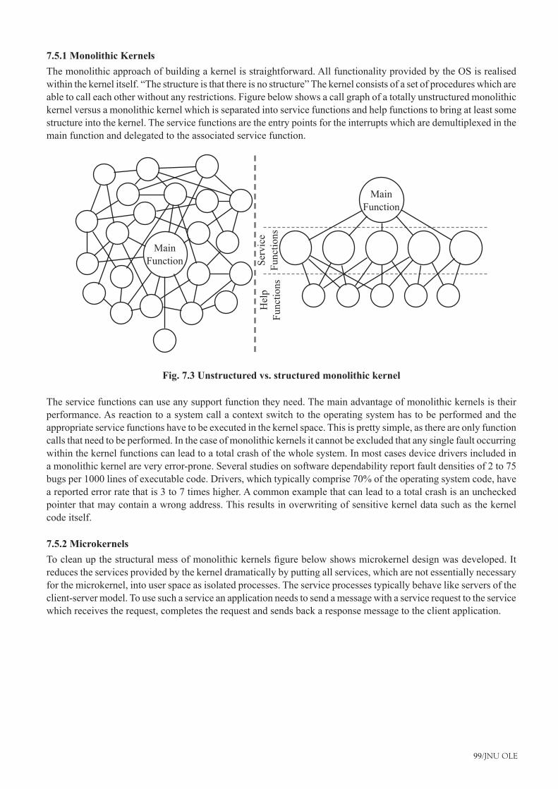
99/JNU OLE

7.5.1 Monolithic KernelsThe monolithic approach of building a kernel is straightforward. All functionality provided by the OS is realised within the kernel itself. “The structure is that there is no structure” The kernel consists of a set of procedures which are able to call each other without any restrictions. Figure below shows a call graph of a totally unstructured monolithic kernel versus a monolithic kernel which is separated into service functions and help functions to bring at least some structure into the kernel. The service functions are the entry points for the interrupts which are demultiplexed in the main function and delegated to the associated service function.

Main Function

Main Function

Hel

p Fu

nctio

nsSe

rvic

e Fu

nctio

ns

Fig. 7.3 Unstructured vs. structured monolithic kernel

The service functions can use any support function they need. The main advantage of monolithic kernels is their performance. As reaction to a system call a context switch to the operating system has to be performed and the appropriate service functions have to be executed in the kernel space. This is pretty simple, as there are only function calls that need to be performed. In the case of monolithic kernels it cannot be excluded that any single fault occurring within the kernel functions can lead to a total crash of the whole system. In most cases device drivers included in a monolithic kernel are very error-prone. Several studies on software dependability report fault densities of 2 to 75 bugs per 1000 lines of executable code. Drivers, which typically comprise 70% of the operating system code, have a reported error rate that is 3 to 7 times higher. A common example that can lead to a total crash is an unchecked pointer that may contain a wrong address. This results in overwriting of sensitive kernel data such as the kernel code itself.

7.5.2 MicrokernelsTocleanupthestructuralmessofmonolithickernelsfigurebelowshowsmicrokerneldesignwasdeveloped.Itreduces the services provided by the kernel dramatically by putting all services, which are not essentially necessary for the microkernel, into user space as isolated processes. The service processes typically behave like servers of the client-server model. To use such a service an application needs to send a message with a service request to the service which receives the request, completes the request and sends back a response message to the client application.


100/JNU OLE

Client Process

1

Client Process

n

µ-Kernel

Memory Server

Network driver User mode

Supervisor mode

Fig. 7.4 Microkernel architecture

The big question is which services are not essentially necessary for the microkernel. The common approach puts the following services into the microkernel itself: Dispatcher, Scheduler, and Memory Manager. Whether it is necessary to put the memory manager into the microkernel is a topic that has been discussed for a long time without any general agreement. However some memory management for the kernel objects itself is needed within the microkernel. The big advantage of microkernels against monolithic kernels is the clear separation of services from the kernel itself making the kernel a very small piece of software that provides a better fault isolation and can be maintained more easily than a monolithic kernel. The fault isolation prevents crashing the whole system. Even if for example, a driver located in user space fails it is not possible for the driver to manipulate any kernel sensitive data like the kernel code.

The price we have to pay for the better structuring and fault isolation is that we get a high amount of interprocess communication through message passing and a high amount of context switching. The reason for this is that for every system call at least two messages have to be sent and four context switches have to be performed. This is illustratedinthefigurebelow.

Client

context switch

context switch

µ-Kernel Server

request message

response message

context switch

context switch

Fig. 7.5 Client/Server IPC

In contrast to monolithic kernels we also have to deal with an impact on the real-time behaviour, because now system calls are not necessarily executed at the time they have been initiated. The reason is that the services behave like regular processes that have to be scheduled by the real-time scheduler. There are several approaches to deal with that problem. A very simple one is to use priority message queues for the service requests within the server and to apply priority inheritance on the server processes to guarantee that no unbound blocking time can occur.

101/JNU OLE

7.5.3 Virtual Machines and ExokernelsThe main idea of system virtual machines is to provide an exact copy of the available hardware for every virtual machine. Therefore a small control program is necessary to assign the available hardware to the virtual machines. This program is called the virtual machine monitor (VMM) or hypervisor. This program is the only code executed in supervisor mode and ensures that the virtual machines are clearly isolated from each other.

P1

OS1

Virtual Machine Monitor

Hardware

OS2 OSn User mode

Supervisor mode

P1 P1Pn Pn Pn

Fig. 7.6 Virtual machine monitor

Thebiggestissuetobesolvedisthequestionwhethervirtualisationcanbeachievedefficiently.Toanswerthisinstruction set architecture (ISA) plays the most important role. The ISA is divided into sensitive and innocuous instruction. Sensitive instructions interact with hardware and need to cause a trap to activate the VMM. Innocuous instruction can be executed natively if possible (provided that the ISAs of the host and the virtual machine are identical). If instructions cannot be executed natively they need to be emulated. For emulation the target code to be executed on a different host ISA needs to be transformed before it can be executed. The question whether an efficientVMMcanbebuiltisreducedtothequestionwhetherthesetofsensitiveinstructionsisasubsetofthesetofprivilegedinstructionsasshowninfigurebelow.

Nonprivileged

Privileged

Sensitive

PrivilegedSensitive

Innocuous

Fig. 7.7 Efficiency classification of ISAs

Exokernels are very similar to virtual machine monitors, but they differ in the way that exokernels do not provide an exact copy of the available hardware.

Instead they partition the available resources and assign them to the virtual machines running on top of the exokernel. A good example is the main memory of the system. VMMs provide an exact copy of the complete main memory to the virtual machines running on top of the VMM. The VMM needs to map the memory of every virtual machine to the real physical memory. Exokernels do not have to manage such a mapping as the different virtual machines would have only access to disjoint subsets of the available physical memory.


102/JNU OLE

7.6 RTOS for Safety Critical SystemsComputer systems that operate systems of critical responsibility are called safety-critical systems. Typically, a small deviation in the environment or the system’s behaviour, a failure or an error appearing within such a system can yield in hazardous situations and may cause catastrophes. Safety-critical systems therefore must not only guarantee real-time behaviour but further more they require absolute dependability and availability of system service. To free application developers from implementing safety and real-time mechanisms into each application, operating systems serve as the underlying platform designed towards supporting real-time and all safety-incorporating non-functional features. Because of the critical consequences of a system failure, standards are required to specify the design and thedevelopmentprocess.Theydefinethemethodsandtechniquesthatarerequiredtopreventsystemfailuresandenforce a state-of-the-art quality-of-service in safety-critical applications.

Two relevant standards exist: IEC 61508 and DO-178B. The title of the international standard IEC 61508 is “Functional safety of electrical/electronic/programmable electronic safety-related systems”. It is a generic safety standardthatformsthebasisformanyother—domainspecific—standards.Thisstandarddefinesrequirementsonthelifecycleofsafety-relatedsystems,fromsystemdevelopmenttoitsoperation.Itidentifiesmeasuresandtechniquesfor preventing failures and contains methods for controlling possible system failures. DO-178Bis titled “Software ConsiderationsinAirborneSystemsandEquipmentCertification”andspecifiesguidelinesforthedevelopmentofavionic software. It builds up a stringent application-dependent safety standard.

As recent trends are heading towards the integration of applications of different criticality levels on one single platform, operating systems for safety critical applications face the challenge of guaranteeing the availability of the processor time as well as the availability of resources (full protection in time and in space domain). These challenges must be inherently incorporated into the RTOS architecture. The Avionics industry formulated these architecturalrequirementsintheARINC653specificationtoguidemanufacturersofavionicapplicationsoftwaretowards maximum standardisation.

7.7 Protection in Time DomainRunning multiple applications with different criticality levels on one processor may lead to no provision for guaranteeing processor time for critical applications. Consider the following scenario: Two applications of different criticality levels, each with one thread at the same priority run on a single system. Thread 1 is a non-critical thread whereas thread 2 is a critical one that needs at least 45% of the processor time to process its workload. As the two threads get assigned the same priority, a scheduler will assign each of the threads 50%of the processor time. In that case, the critical thread 2 will get its work done. Suppose that thread 1 spawns a new thread with the same priority. Then, the scheduler handles three threads at the same priority. As a consequence each of the threads will get only 33% of the processor time. Hence, the critical thread2 is not able to handle its workload any more. The requirement of protection in time domain results clearly from this example.

7.8 Protection in Space DomainDue to predictability reasons, many RTOS designers do not use virtual memory management. The fact that multiple applications with different criticality levels run on one single processor involves that processes share the same memory space. This implies that a process is able to corrupt the code, data or the stack of another process, intentionally or unintentionally. Furthermore, a process can also corrupt data or code of the operating system kernel which affects the safety and reliability of the system. In fact, it can lead to unexpected system behaviour that infects the predictability and it can even bring down the entire system. Therefore, the protection of the memory is one key issue in RTOS for safety critical systems.

7.9 Secure Operating System ArchitectureTheanswertotherequirementofprotectionisanarchitecturethatdefinesafullyandsecurelypartitionedreal-time operating system. The partitioning is carried out also in two dimensions: Spatial Partitioning and Temporal Partitioning.

103/JNU OLE

In particular, the basic design of such an operating system complies with the design of an ordinary RTOS. The fundamental difference is located above the operating system’s core layer within the application layer which in fact is a construction of several separate partitions of the ordinary application layer. Each partition is assigned to an integrity level only allowing the running of applications compliant to this level. Furthermore, it consists of a small Partition Operating System that provides operating system services according to the safety features required by the safety integrity level. Furthermore, the Partition OS in fact runs the proper applications. The operating system core layer is responsible for the hardware-dependent functions, the device drivers, the scheduler, and so on.

Application #1

Partition OS

OS Core

Processor

Ports Scheduler

Partition OS

Partition OS

Application #2

Application #3

Fig. 7.8 OS architecture for safety critical systems


104/JNU OLE

Summary Most embedded systems are bound to real-time constraints.•“Real-time” means that the IT system is no longer controlling its own time domain.•Kopetzdefinesreal-timesystemsas“Areal-timecomputersystemisacomputersysteminwhichthecorrectness•of the system behaviour depends not only on the logical results of the computation, but also on the physical instant at which these results are produced.An operating system, which is capable of taking care of this is called a “Real-time Operating System •(RTOS)”. Real-time systems can be characterised by the strictness of real-time restrictions.•ARTtaskiscalledfirmifmissingitsdeadlinemakestheresultuseless,butmissingdoesnotcauseserious•damage.Periodictasksreflectdirectlythe“sense–execute–act”loopincontrolapplications.•Running multiple applications with different criticality levels on one processor may lead to no provision for •guaranteeing processor time for critical applications.

ReferencesRammig, F., Ditze, M., Janacik, P., Heimfarth, T., Kerstan,T., Oberthuer, S. & Stahl, K., • Basic Concepts of Real Time Operating Systems, [pdf]Available at: <http://www.springer.com/cda/content/document/cda_downloaddocument/9781402094354-c2.pdf?SGWID=0-0-45-699603-p173865105> [Accessed 31 July 2012].Pettersson, M., • Basic Concepts for Real Time Operating Systems, [pdf] Available at: <http://www.iar.com/Global/Resources/Developers_Toolbox/RTOS_and_Middleware/Basic_Concepts_for_Real_Time_Operating_Systems.pdf>[Accessed 31 July 2012].2012. lec 38 - • Real Time Operating Systems for Embedded Applications, [Video Online] Available at: <http://www.youtube.com/watch?v=rpdygqOI9mM> [Accessed 31 July 2012].2011. • About Real-Time Operating Systems, [Video Online] Available at: <http://www.youtube.com/watch?v=luny1VaV4AI&feature=results_main&playnext=1&list=PL1E4FAC247DD27FC5> [Accessed 31 July 2012].Kamal, R., 2008. • Embedded Systems, 2nd ed., Tata McGraw-Hill Education.Barrett, • Embedded Systems, Pearson Education India.

Recommended ReadingKopetz, H., 2011. • Real-Time Systems: Design Principles for Distributed Embedded Applications (Real-Time Systems Series), 2nd ed., Springer.Li, Q. & Caroline Yao, C., 2003. • Real-Time Concepts for Embedded Systems, 1sr ed., CMP.Sheppard, T., 2011. • Real-Time Embedded Systems Fundamentals, 1st ed., Surreal-Time Ltd.

105/JNU OLE

Self Assessment A__________taskiscalledfirmifmissingitsdeadlinemakestheresultuseless,butmissingdoesnotcause1. serious damage.

RTa. RTLb. TTLc. DTLd.

An operating system which is capable of taking care of this is called a ___________.2. Digital Operating Systema. Real-time Operating System b. Index Operating Systemc. Analog Operating Systemd.

____________definesreal-timesystemsas“Areal-timecomputersystemisacomputersysteminwhichthe3. correctness of the system behaviour depends not only on the logical results of the computation, but also on the physical instant at which these results are produced".

Henrya. Edward b. Kopetzc. Petterssond.

Which of the following statements is true?4. Non-periodictasksreflectdirectlythe“sense–execute–act”loopincontrolapplications.a. Dynamictasksreflectdirectlythe“sense–execute–act”loopincontrolapplications.b. Statictasksreflectdirectlythe“sense–execute–act”loopincontrolapplications.c. Periodictasksreflectdirectlythe“sense–execute–act”loopincontrolapplications.d.

__________ systems can be characterised by the strictness of real-time restrictions.5. Real-timea. ITb. Digital c. Analogd.

__________ means that the IT system is no longer controlling its own time domain.6. Periodica. Real-timeb. Non-periodicc. Dynamicd.

___________ means that the correctness of the system depends not only on logical results but also on the time 7. the results are produced.

Intervala. Interrupt b. Timec. Space d.


106/JNU OLE

Which of the following statements is true?8. Most embedded systems are not bound to real-time constraints.a. Most real time systems are bound to real-time constraints.b. Most embedded systems are bound to embedded constraints.c. Most embedded systems are bound to real-time constraints.d.

A RT task is called __________ if meeting its deadline is desirable but missing does not cause serious 9. damage.

softa. hardb. firmc. missing d.

The main advantage of __________ kernels is their performance.10. Minikernelsa. Monolithicb. Microkernelsc. Exokernelsd.

107/JNU OLE

Chapter VIII

Validation

Aim


introduce the concept of validation in embedded systems•

elucidate simulation•

explain rapid prototyping and emulation•

Objectives


explain fault simulation•

explicate risk- and dependability analysis•

elucidateformalverification•

Learning outcome


understand fault injection•

identify fault tree analysis•

recognise failure mode a• nd effect analysis


108/JNU OLE

8.1 IntroductionOne very important aspect of embedded system design has not been considered so far: validation. Validation is the process of checking whether or not a certain (possibly partial) design is appropriate for its purpose meets all constraints and will perform as expected. Validation is important for any design procedure, and hardly any system would work as expected, had it not been validated during the design process. Validation is extremely important for safety-critical embedded systems.

Intheory,wecouldtrytodesignverifiedtoolswhichalwaysgeneratecorrectimplementationsfromthespecification.Inpractice,thisverificationoftoolsdoesnotwork,exceptinverysimplecases.Asaconsequence,eachandeverydesignhastobeverified.Inordertominimisethenumberoftimesthatwehavetoverifyadesign,wecouldtryto verify it at the very end of the design process. Unfortunately, this approach normally does not work, due to the largedifferencesbetweenthelevelofabstractionusedforthespecificationandthatusedfortheimplementation.Therefore, validation is required at various phases during the design procedure. Validation and design should be intertwined and not be considered as two completely independent activities.

It would be nice to have a single validation technique applicable to all validation problems. In practice, none of the available techniques solves all the problems, and a mix of techniques has to be applied. In this chapter, we will provide a brief overview over the key techniques which are available.

specification

standard software





...

hardware

egdelwonk noitacilppa


8.2 SimulationSimulations are a very common technique for validating designs. Simulations consist of executing a design model on appropriate computing hardware, typically on general purpose digital computers. Obviously, this requires models to be executable. All the executable languages can be used in simulations, and they can be used at various levels. The level at which designs are simulated is always a compromise between simulation speed and accuracy. The faster the simulation, the less accuracy is available.

So far, we have used the term behaviour in the sense of the functional behaviour of systems (its input/output behaviour). There are also simulations of some non-functional behaviour of designs, including the thermal behaviour and the electro-magnetic compatibility (EMC) with other electronic equipment. For embedded systems, simulations have serious limitations:

Simulations are typically a lot slower than the actual design. Hence, if we tried to interface the simulator with •the actual environment, we would have quite a number of violations of timing constraints.Simulations in the real environment may even be dangerous (who would want to drive a car with unstable •control software?).

109/JNU OLE

For many applications, there may be huge amounts of data and it may be impossible to simulate enough data •in the available time. Multimedia applications are notoriously known for this. For example, simulating the compression of some video stream takes an enormous amount of time.Most actual systems are too complex to allow simulating all possible cases (inputs). Hence, simulations can help •ustofinderrorsinourdesigns.Theycannotguaranteeabsenceoferrors,sincesimulationscannotexhaustivelybe done for all possible combinations of inputs and internal states.Duetothelimitations,thereisanincreasedemphasisonformalverification.•

8.3 Rapid Prototyping and EmulationTherearemanycasesinwhichthedesignsshouldbetriedoutinrealisticenvironmentsbeforefinalversionsaremanufactured. Control systems in cars are an excellent example for this. Such systems should be used by drivers in different environments before mass production is started. Accordingly, the car industry designs prototypes. These prototypesshouldessentiallybehavelikethefinalsystems,buttheymaybelarger,morepowerconsumingandhave other properties which test drivers can accept. Such prototypes can be built, for example, using FPGAs. Racks containing FPGAs can be stored in the trunk while test drivers exercise the car.

This approach is not limited to the car industry. There are several other cases in which prototypes are built from FPGAs. Commercially available emulators consist of a large number of FPGAs. They come with the required mapping toolswhichmapspecificationstotheseemulators.Usingtheseemulators,experimentswithsystems,whichbehave“almost”likethefinalsystemscanberun.

8.4 TestScopeIn testing, we are applying a set of specially selected input patterns, so-called test patterns to the input of the system, observe its behaviour and compare this behaviour with the expected behaviour. Test patterns are normally applied to the real, already manufactured system. The main purpose of testing is to identify systems that have not been correctlymanufactured(manufacturingtest)andtoidentifysystemsthatfaillater(fieldtest).

Testing includes a number of different actionsTest pattern generation•Test pattern application•Response observation, and•Result comparison.•

In test pattern generation, we try to identify a set of test patterns which distinguish correctly working from incorrectly working systems. Test pattern generation is based on fault models. Such fault models are models of possible faults. For example, it is possible to use the stuck-at-fault model, which is based on the assumption, that any internal wire of an electronic circuit is either permanently connected to ’0’ or ’1’ (this is the so-called stuck-at model). It has been observed that many faults actually behave as if some wire was permanently connected that way. However, recent CMOS technologies require more comprehensive fault models. These include transient faults and delay faults (faults changing the delay of a circuit) explicitly. While good fault models exist for hardware testing, the same is not true for software testing. Test pattern generation tries to generate tests for all faults that are possible according to a certain fault model. The quality of the test pattern set can be evaluated using the fault coverage. Fault coverage is the percentage of potential faults that can be found for a given test pattern set:

Coverage =


110/JNU OLE

In practice, achieving a good product quality requires fault coverage’s in the area of 98 to 99 %. In order to increase the number of options that exist for system validation, it has been proposed to use test methods already during the design phase. For example, test pattern sets can be applied to software models of systems in order to check if two software models behave in the same way. More time consuming formal methods need to be applied only to those cases in which this test-based equivalence check did not fail.

Design for testabilityIftestingcomesinonlyasanafterthought,itmaybeverydifficulttotestasystem.Forexample,verifyingwhetherornottwofinitestatemachinesareequivalentmayrequirecomplexhomingsequences(sequencesreturningtheFSM to some initial state). In order to simplify tests, special hardware can be added such that testing becomes easier. The process of designing for better testability is called design for testability, or DfT. Special purpose hardware for testingfinitestatemachinesisaprominentexampleofthis.Reachingcertainstatesandobservingstatesresultingfromtheapplicationofinputpatternsareverymuchsimplifiedwithscandesign.Inscandesign,allflip-flopsstoringstates are connected to form serial shift registers.

Z2+

Z2

Z1+

Z1

Z0+

Z0

mux

mux

mux

X

Y+

network

Z = (X,Z)Y= (X,Z)

normal mode/ test modeinputserial

serial output

Fig. 8.2 Scan path design

Settingthemuxtoscanmode,wecanloadanystateintothethreeflip-flopsserially.Inasecondphase,wecanapplyinput patterns to the FSM while the mux are set to normal mode. As a result, the FSM will be in a new state.

Thisnewstatecanbeseriallyshiftedoutinthethirdandfinalphase,usingtheserialmodeagain.TheneteffectisthatwedonotneedtoworryabouthowtogetintocertainstatesandhowtoobservewhetherornotδhasbeencorrectlyimplementedwhilewearegeneratingtestsfortheFSM.AsafewayoftestingFSMtransitionsistofirstshiftthe“old”stateintotheshiftregisterchain,thentoapplytheinput,andfinallytoshifttheresultingnewstateout of the scan chain. Effectively, the fact that we are dealing with state-based systems has an impact only on the two (simple) shift phases, and test pattern generation for (stateless) Boolean networks can be used for checking for correctoutputs.ThismeansthatitissufficienttousetestpatterngenerationmethodsforBooleanfunctions(statelessnetworks) instead of caring about homing sequences etc.

Scan design is a technique which works well for single chips. For board-level integration it is necessary to have some technique for connecting scan chains of several chips. JTAG is a standard, which does exactly this. The standard definesregistersattheboundariesofallchipsandanumberoftestpinsandcontrolcommandssuchthatallchipscan be connected in scan chains. JTAG is also known as boundary scan.

111/JNU OLE

Forchipswithalargenumberofflip-flops,incantakequitesometimetosetandreadallofthem.Inordertospeedup the process of generating patterns on the chip, it has been proposed to also integrate hardware for generating test patterns on the chip. Typically pseudo-random patterns, generated by registers with feed-back paths are used as test patterns.

In order to also avoid shifting out the response of the circuit under test, responses are compacted. Compacted responses behave very much like cyclic redundancy check (CRC) characters in that the probability of generating correctcompactedtestresponsesfromanincorrectresponsecanbemadeverylow(about2−nwherenisthenumberof bits in the compacted response).

The built-in logic block observer (BILBO) has been proposed as a circuit combining test pattern generation, test responsecompactionandserialinput/outputcapabilities.ABILBOwiththreeD-typeflip-flopsisshowninfigurebelow.

outputserial

Z

DQ

Z

DQ

1 2

11

2

2

c

Z 0

D0Q0

mux norxor

01

2

c1

clock

inputserial

Fig. 8.3 BILBO

ModesofBILBOregistersareshownintable8.1.The3-bitregistershowninfigureabovecanbeinscanpath,reset, linear-feedback shift register (LFSR) and normal mode. In LFSR mode, it can be used for either generating pseudorandom pattern or for compacting responses from inputs (Z0 to Z2).

Typically, BILBOs are used in pairs. One BILBO generates pseudo-random test patterns, feeding some Boolean network with these patterns. The response of the Boolean network is then compressed by a second BILBO connected to the output of the network. At the end of the test sequence, the compacted response is serially shifted out and compared with the expected response.

c1 c2 Di’0’ ’0’ 0 ⊕Qi 1 = Qi 1 scan path mode’0’ ’1’ 0 ⊕ 1 = 0 reset’1’ ’0’ Zi⊕Qi 1 LFSR mode’1’ ’1’ Zi⊕ 1 = Zi normal mode

Table 8.1 Mod es of BILBO


112/JNU OLE

DfT hardware is of great help during the prototyping and debugging of hardware. It is also useful to have DfT hardwareinthefinalproduct,sincehardwarefabricationneverhasazerodefectrate.Testingfabricatedhardwaresignificantlycontributestotheoverallcostofaproductandmechanismsthatreducethiscostarehighlyappreciatedby all companies.

Self-test programsOne of the key problems of testing modern integrated circuits is their limited number of pins, making it more and moredifficulttoaccessinternalcomponents.Also,it isgettingverydifficulttotestthesecircuitsatfullspeed,since testers must be at least as fast as the circuits themselves. The fact that many embedded systems are based on processors provides a way out of this dilemma: processors are capable of running test programs or diagnostics. Such diagnostics have been used to test main frame machines for decades. Figure below shows some components that might be contained in some processor.

instructionregister

registerfile

ALU

Fig. 8.4 Segment from processor hardware

The types of faults that are considered are part of the fault model. In order to test for stuck-at-faults at the input of the ALU, we can execute a small test program:storepatternofall’1’sinregisterfile;perform xor between constant “0000...00” and register,test if result contains ’0’ bit,if yes, report error;otherwise start test for next stuck-at-fault

Similar small programs can be generated for other stuck-at-errors. Unfortunately, the process of generating diagnostics for main frames has mostly been a manual one. Some researchers have proposed to generate diagnostics automatically.

8.5 Fault SimulationIt is currently not feasible (and it will probably not be feasible) to completely predict the behaviour of systems in the presence of faults. Therefore, the behaviour of systems in the presence of faults is frequently simulated. This type ofsimulationiscalledfaultsimulation.Infaultsimulation,systemmodelsaremodifiedtoreflectthebehaviourofthe system in the presence of a certain fault. The goals of fault simulation include:

To know the effect of a fault of the components at the system level. Faults are called redundant if they do not •affect the observable behaviour of the system, andTo know whether or not mechanisms for improving fault tolerance actually helps.•

Fault simulation requires the simulation of the system for all faults feasible for the fault model and also for a possibly large number of different input patterns. Accordingly, fault simulation is an extremely time-consuming process. Different techniques have been proposed to speed up fault simulation. These techniques include parallel fault simulation. Parallel fault simulation is especially effective if the system is modelled at the gate level. In this case, internal signals are single bit signals.

113/JNU OLE

This fact enables the mapping of a signal to a single bit of some machine word of a simulating host machine. AND- and OR machine instructions can then be used to simulate Boolean networks. However, only a single bit would be usedpermachineword.Efficiencyisimprovedwithparallelfaultsimulation.Inparallelfaultsimulation,ndifferenttest patterns are simulated at the same time, if n is the machine word size. The values of each of the n test patterns are mapped to a different bit position in the machine word. Executing the same set of AND- and OR-instructions will then simulate the behaviour of the Boolean network for n test patterns instead of for just one.

8.6 Fault InjectionFault simulation may be too time-consuming for real systems. If actual systems are available, fault injection can be usedinstead.Infaultinjection,realexistingsystemsaremodifiedandtheoveralleffectonthesystembehaviouris checked.

Fault injection does not rely on fault models (even though they can be used). Hence, fault injection has the potential of generating faults that would not have been predicted by a fault model. We can distinguish between two types of fault injection: local faults within the system, and faults in the environment (behaviours which do not correspond tothespecification).

Forexample,wecancheckhowthesystembehavesifitisoperatedoutsidethespecifiedtemperatureorradiationranges.

Several methods can be used for fault injection:Fault injection at the hardware level: Examples include pin-manipulation, electromagnetic and nuclear •radiation.Fault injection at the software level: Examples include toggling some memory bits.•

According to experiments software-based fault injection was essentially as effective as hardware-based fault injection. Nuclear radiation was a noticeable exception in that it generated errors which were not generated with other methods.

8.7 Risk and Dependability AnalysisEmbedded systems (like many products) can cause damages to properties and lives. It is not possible to reduce the risk of damages to zero. The best that we can do is to make the probability of damages small, hopefully orders of magnitudesmallerthanotherrisks.Formanyapplications,aprobabilityofacatastrophehastobelessthan10−9per hour corresponding to one case per 100,000 systems operating for 10,000 hours. Damages are resulting from hazards.Foreachpossibledamagethereisaseverity(thecost)andaprobability.Riskcanbedefinedastheproductof the two.

Risks can be analysed with several techniques:

Fault tree analysis (FTA)FTA is a top-down method of analysing risks. The analysis starts with a possible damage and then tries to come up with possible scenarios that lead to that damage. FTA typically uses a graphical representation of possible damages, including symbols for AND- and OR gates.

OR-gates are used if a single event could result in a hazard. AND gates are used when several events or conditions are required for that hazard to exist. Figure below shows an example.


114/JNU OLE

User receives mail

No firewall used

TCP/IP port open + OS bug

User clicks on attachment

PC connected to internet

Floppy includes boot virus

Floppy in drive at boot time

Attachment has virus

Boot sequence checks floppy

OS hazard

.....

AND

OR

Fig. 8.5 Fault tree

The simple AND- and OR-gates cannot model all situations. For example, their modelling power is exceeded if shared resources of some limited amount (like energy or storage locations) exist. Markov models may have to be used to cover such cases.

Failure mode and effect analysis (FMEA)FMEA starts at the components and tries to estimate their reliability. Using this information, the reliability of the systemiscomputedfromthereliabilityofitsparts(correspondingtoabottom-upanalysis).Thefirststepistocreatea table containing components, possible faults, probability of faults and consequences on the system behaviour. Risks for the system as a whole are then computed from the table. Table 8.2 shows an example 2.

Tools supporting both approaches are available. Both approaches may be used in “safety cases”. In such cases, an independent authority has to be convinced that certain technical equipment is indeed safe. One of the commonly requested properties of technical systems is that no single failing component should potentially cause a catastrophe.

Component Failure Consequences Probability Critical?Processor metal migration no service 10 6 /h yes... ... ... ... ...

8.8 Formal VerificationFormalverificationisconcernedwithformallyprovingasystemcorrect,usingthelanguageofmathematics.Firstofall,aformalmodelisrequiredtomakeformalverificationapplicable.Thisstepcanhardlybeautomatedandmay require some effort. Once the model is available, we can try to prove certain properties.

Formalverificationtechniquescanbeclassifiedbythetypeoflogicsemployed:

Propositional logicIn this case, models consist of Boolean formulas described with Boolean variables and connectives such as and or. (Stateless) gate-level logic networks can be conveniently described with propositional logic. Tools typically aim at checking if two models represented this way are equivalent. Such tools are called tautology checkers or equivalence checkers. Since propositional logic is decidable, it is also decidable whether or not the two representations are equivalent (there will be no cases of doubt). For example, one representation might correspond to gates of an actual circuitandtheothertoitsspecification.

115/JNU OLE

Proving the equivalence then proves the effect of all design transformations (for example, optimisations for power or delay) to be correct. Tautology checkers can frequently cope with designs which are too large to allow simulation-based exhaustive validation.

The key reason for the power of recent tautology checkers is the use of Binary Decision Diagrams (BDDs). The complexity of equivalence checks of Boolean functions represented with BDDs is linear in the number of BDD-nodes. In contrast, the equivalence check for functions represented by sums of products is NP-hard. Still, the number of BDD-nodesrequiredtorepresentacertainfunctionhastobetakenintoaccount.Manyfunctionscanbeefficientlyrepresented with BDDs. In the general, however, the number of nodes of BDDs grows exponentially with the number ofvariables.InthosecasesinwhichfunctionscanbeefficientlyrepresentedwithBDDs,BDD-basedequivalencecheckers have frequently replaced simulators and are used to verify gate networks with millions of transistors. The abilitytoalsoverifyfinitestate-machinesisverymuchlimited.

First order logic (FOL)FOLincludesquantification,using∃ and ∀. Some automation for verifying FOL models is feasible. However, since FOL is undecidable in general, there may be cases of doubt. Higher order logic (HOL): Higher order allows functions to be manipulated like other objects. For higher order logic, proofs can hardly ever be automated and typically must be done manually with some proof-support.

Model checkingVerificationoffinitestatemachinescanbeperformedwithmodelchecking.Modelcheckingaimsattheverificationofpropertiesoffinitestatesystems.Itanalysesthestatespaceofthesystem.Verificationusingthisapproachrequiresthree stages:

thegenerationofamodelofthesystemtobeverified•thedefinitionofthepropertiesexpectedfromthesystem,and•modelchecking(theactualverificationstep)•

Accordingly, model checking systems accept the model and properties as input.

state transition preprocessing

proof orcounterexample

graph

Model checker

properties

Fig. 8.6 Inputs for model checking

Verification tools canproveordisprove theproperties. In the latter case, theycanprovidea counter-example.ModelcheckingiseasiertoautomatethanFOL.Languagesusedforthedefinitionofpropertiestypicallyallowthequantificationofstates.


116/JNU OLE

A popular system for model checking is Clarke’s EMC-system. This system accepts properties to be described as CTL formulas.

CTL stands for “Computational Tree Logics”. CTL-formulas include two parts:apathquantifier(thispartspecifiespathsinthestatetransitiondiagram),and•astatequantifier(thispartspecifiesstates)•

Example: M, s |= AGg means: In the transition graph M, property g holds for all paths (denoted by A) and all states (denotes by G).

In1987,modelcheckingwasimplementedusingBDDs.Itwaspossibletolocateseveralerrorsinthespecificationof the future bus protocol. Extensions are needed in order to also cover real-time behaviour and numbers. More informationonformalverificationcanbefoundinbooksonthistopic.

117/JNU OLE

Summary Validation is the process of checking whether or not a certain (possibly partial) design is appropriate for its •purpose meets all constraints and will perform as expected.Validation is important for any design procedure, and hardly any system would work as expected, had it not •been validated during the design process.Validation and design should be intertwined and not be considered as two completely independent activities.•Simulations consist of executing a design model on appropriate computing hardware, typically on general •purpose digital computers.In testing, we are applying a set of specially selected input patterns, so-called test patterns to the input of the •system, observe its behaviour and compare this behaviour with the expected behaviour.In test pattern generation, we try to identify a set of test patterns which distinguish correctly working from •incorrectly working systems.Formalverificationisconcernedwithformallyprovingasystemcorrect,usingthelanguageofmathematics.•FTA typically uses a graphical representation of possible damages, including symbols for AND- and OR •gates.In fault injection, real existing systems aremodified and the overall effect on the system behaviour is•checked.Fault simulation requires the simulation of the system for all faults feasible for the fault model and also for a •possibly large number of different input patterns.

ReferencesMarwedel, P., 2010. • Embedded System Design, 2nd ed., Springer.Barrett, • Embedded Systems, Pearson Education India.Roychoudhary, A., • Embedded Systems and Software Validation, [pdf] Available at: <http://www.comp.nus.edu.sg/~abhik/Book/Preface_and_TOC.pdf> [Accessed 18 July 2012].Bondavalli, A., Fantechi, A., Latella, D. & Simoncini, L., • Design Validation of Embedded Dependable systems, [pdf] Available at: <http://fmt.isti.cnr.it/WEBPAPER/MICRO01Latella.pdf> [Accessed 18 July 2012].Dr. Chaudhury, S., • 2008. Lecture -1 Embedded Systems: Introduction, [Video Online] Available at: <http://www.youtube.com/watch?v=y9RAhEfLfJs&playnext=1&list=PL85B2CDE655D0D63C&feature=results_main> [Accessed 31 July 2012].2008, • Lecture -1 Embedded Systems: Introduction, [Video Online] Available at: <http://www.youtube.com/watch?v=y9RAhEfLfJs> [Accessed 4 July 2012].

Recommended ReadingRoychoudhary, A. 2009. • Embedded Systems and Software Validation, 1st ed., Morgan Kaufmann.Nicolescu, G. & Jerraya, A. A., 2007. • GlobalSpecificationandValidationofEmbeddedSystems:IntegratingHeterogeneous Components, 1st ed., Springer.Baron, J., Geffroy, J. C. & Motet, G., 1997. • Embedded System Applications, 1st ed., Springer.


118/JNU OLE

Self Assessment__________ is the process of checking whether or not a certain (possibly partial) design is appropriate for its 1. purpose meets all constraints and will perform as expected.

Evaluationa. Verificationb. Testingc. Validationd.

____________ is important for any design procedure, and hardly any system would work as expected, had it 2. not been validated during the design process.

Validationa. Evaluationb. Verificationc. Testingd.

Which of the following statements is true?3. Validation and design should be intertwined and be considered as two completely independent activities.a. Validation and design should be intertwined and not be considered as two completely independent b. activities.Validation and design should be intertwined and not be considered as two completely dependent c. activities.Validation and design should be intertwined and be considered as two completely dependent activities.d.

Which of the following consist of executing a design model on appropriate computing hardware, typically on 4. general purpose digital computers?

Simulationsa. Evaluationb. Validationc. Testingd.

In __________ generation, we try to identify a set of test patterns which distinguish correctly working from 5. incorrectly working systems.

test patterna. reportb. faultc. input patternd.

____________ verification is concernedwith formally proving a system correct, using the language of6. mathematics.

Formala. Informalb. Testc. Fault d.

119/JNU OLE

____________ typically uses a graphical representation of possible damages, including symbols for AND- and 7. OR gates.

FTAa. CTLb. FMEAc. BDDd.

In____________ , real existing systems aremodified and the overall effect on the systembehaviour is8. checked.

test patterna. fault injectionb. soft computingc. fault simulationd.

___________ requires the simulation of the system for all faults feasible for the fault model and also for a 9. possibly large number of different input patterns.

Fault simulationa. Test patternb. Fault injectionc. Soft computingd.

__________ is a top-down method of analysing risks.10. FTAa. CTLb. FMEAc. BDDd.


120/JNU OLE

Application I

Liquid level Controller

Abstract: Keeping the liquid up to certain level in tank is one of the widely used applications in petroleum and consumable goods producing industries. Certain amount of liquid should be always there in the tank to keep the liquid pressure as it is. To maintain this level there is a need of liquid level controller.

It’s a close loop control system. It may be ON-OFF type of or continuous type system. There are two valves in tank. Oneisinletandotherisoutlet.Ifonewantsconstantflowofliquidfromtankthenoutletvalvemustbefullyopenandliquidlevelinthetankshouldbeaboveminimumspecifiedlimit.Andthislimitismaintainedbycontrollingflowfrominletvalve.

ON-OFF type: In this system there are two limits. 1) max limit 2) min limit. If liquid level goes beyond max limit then inlet valve is closed. Now as outlet valve is fully open the liquid level will start decreasing. As it reaches min limit and go below this inlet valve is again open. So, liquid level will remain within these two limits.

Continuous type: In this system there is only one limit. That is called set value. The liquid level in the tank is continuously compared with this set value. The opening of inlet valve is varied according to the change in the level in tank. Opening becomes wider if level falls and becomes shorter if level goes beyond set value. So, continuous correction is made to maintain set value of level.

Here,isanexampleofverysimplecontrollerinwhichfirstthetankisfilleduptorequiredlevelusingpumpandthenaftersometimeitisflushedcompletelybyreversingpump.Againwhentankisemptythepumpautomaticallystartsfillingtank.Andthiscyclecontinuous.Onecansettherequiredleveleverytimeorhecanchangeitineverycycle. This is demo application in which I am using simulated water tank from multisim software to illustrate this application.

Sofirstletusunderstandtheoperationofthiswatertank.Here,thefiguregivenbelowshowsthearrangementofwater tank with pump and other assembly.

tank

Empty:Target:Sensor:

SP

0%0.00

Total volume: 50.00Set Point: 35.00

Current Volume: 0.00

Pump

Flow-inFlow-outStopflow

Valve

Set level o/p

Tank empty o/p

Analog o/

Flow: 0.00Pump Cntr1Fwd Rev Stop

Fig. 1 The arrangement of water tank with pump and other assembly

121/JNU OLE

Asshowninabovefigurethefullcapacityoftankis50litres.Thesetpoint(requiredlevel)isfixedat35litres.Therateatwhichpumpfillsthetankthatdependsuponvalvesetting.Flowcontrol(whichisnotthepartofthissystem) can be achieved by changing voltage applied at this terminal. There are three inputs to this system that controls pump operation:

flowin-whenitisgivenapositivepulse,waterwillstartflowinginsidetank•flowout-whenitisgivenapositivepulse,waterwillstartflowingoutsidetank•stopflow-whengivenpositivepulseflowwillbestopped•

Three outputs form the system is:setlevel-thiso/pwillbecomehighwhentankisfilleduptosetlevel.Itwillremainhightilllevelismaintained.•As the level decreases o/p becomes lowtankempty-astankisflushedcompletelythiso/pbecomeshigh.Itimmediatelybecomeslowastankstarts•filling.analog o/p - it gives DC o/p 0 - 5 V corresponding to the liquid level in tank. That means 0V when tank is empty •and 5V when tank is full

So actually the system is very simple. Only we have to send pulses to input signals and use the outputs for indications andcontrolactions.Solet’sfirstseetheblockdiagramofthesystem.

Analog o/pTank empty

Set level

f-in f-out stop

ADC 0801

P1 P0

P2P3

89C51

Latch

LED indicators

LCD panel

Buffer

tank &

pump system

Fig. 2 Block diagram of the system

Let us see all the major building blocks one by one 89C51 - This controller chip is the heart of entire system. It receives the inputs from system, it generates suitable outputs to control the system, it displays the data on LCD and indicates various ongoing processes on LEDs

ADC 0801 - It converts analog input 0-5V from system in to digital equivalent.

LCD panel - It displays the liquid level in tank as well as the set point value buffer and latch - they are provided for protection of port pins.

LEDindicators-Theyindicatevariousprocessesgoingonlikewaterflowinside-outsidetank,waterflowstopetc.

So all four ports 89C51 are engaged for various peripheral interfacing.


122/JNU OLE

Fig. 3 Complete schematic diagram of the system connections

ThefiguregivenaboveshowscompleteschematicdiagramofthesystemConnections:TheportP1isconnectedwith digital outputs D0-D7 of ADC. The RC components R2 and C1 forms basic clock circuit for ADC. R3 & R4 forms voltage divider network to generate reference voltage for ADC. The analog output from tank system is directly fed to +Ve input of ADC. Chip select signal CS is tied to gnd. Three control signals RD, WR and INTR of ADC are connected with P3.7, P3.6 and P3.3 respectively. The data pins of LCD are connected with P0 through latch 74LS373. Three control signals RS, RW & En are connected with P2.0, P2.1 and P2.2 respectively. Five LEDs D1 - D5 are connected with P2 pins as shown. Three inputs Fwd, Rev and Stop of tank system are connected to P3.4, P3.5 and P3.0 through buffer IC 74LS07. Tank empty output and set level output are connected with P3.1 and P3.2 through inverter 74LS04. Two LEDs (red and green) are connected for indication of tank empty and set level reached.

Operation: Initially controller displays the set water level on LCD and then applies fwd pulse to pump control. •Sotheliquidwillstartflowinginsidetank.ThisisindicatedbyLEDD2.•Then after every 2 seconds controller will read the liquid level in tank through ADC and displays it as current •water levelNowas the liquid isfilling in tank,when it reaches the set level it sends signal tocontrolleronP3.1and•immediately controller will apply stop pulseNo more liquid is pumped into tank. This is indicated by D3•Thislevelismaintainedfor10seconds.Thencontrollersendsrevpulse.Soliquidwillstartflowingoutside•from the tank. This is indicated by D1.Astankiscompletelyflushed,thetankemptyoutputisgiventocontrollergeneratesaninterrupt.Andimmediately•controller will apply fwd pulseSoagainthepumpwillagainstartfillingtank.Andthiscyclecontinuous.•LEDs D4 and D5 indicates sensing of current liquid level in tank through ADC.•

(Source: Liquid level Controller, [Online] Available at: <http://multyremotes.com/liquid-level-controller.htm> [Accessed 31 July 2012]).

123/JNU OLE

QuestionsMention the two types close loop control systems in the above application.1. AnswerThe two types of close loop control systems are:

ON-OFF type•Continuous type system•

Explain the three inputs to the above system that controls pump operation2. AnswerFollowing are the three inputs to the system that controls pump operation

flowin-whenitisgivenapositivepulse,waterwillstartflowinginsidetank•flowout-whenitisgivenapositivepulse,waterwillstartflowingoutsidetank•stopflow-whengivenpositivepulseflowwillbestopped.•

Explain the three output forms the system 3. AnswerFollowing are the three inputs to the system that controls pump operation

set level - thiso/pwillbecomehighwhen tank isfilledupto set level. Itwill remainhigh till level is•maintained. As the level decreases o/p becomes lowtankempty-astankisflushedcompletelythiso/pbecomeshigh.It immediatelybecomeslowastank•startsfilling.analog o/p - it gives DC o/p 0 - 5 V corresponding to the liquid level in tank. That means 0V when tank is •empty and 5V when tank is full


124/JNU OLE

Application II

Industrial Laser cutting machine

Abstract: - Laser is used to cut different metal sheets, glass, diamond and all other very hard things as this becomes very easy to cut using laser rather then using different blades. It’s one kind of CNC machine in which two stepper motors displaces the laser to calibrated distance. As one enters the dimension of plate (L X B) the system calibrates the linear distance in terms of angular displacement of motor. Then rotates the motor 1 till the length of sheet. Rotate motor 2 till the breadth of sheet. Again rotate motor 1 in reverse direction and then rotate motor 2 in reverse direction to cut complete rectangle (or square).

First let us understand mechanical arrangement for the machine.

Fix supporting

end

Shaft 1

B

Origine

Shaft 2

movable supporting

endgear assembly

Main drive shafts

Motor 1

X-axies (Length)

X-axies (Bredth)

Blank area to insert metal sheet

Fix supporting end B

a

S

Blank area to insert metal sheet

Laser

a

S

Motor 2

Fig. 1 Mechanical arrangement of the machine

Asshowninabovefigure,therearetwosteppermotorsoneistomovelaserhorizontally(motor2)andotheristomove is vertically (motor 1). The angular motion of motor 1 drives 2 main shafts through suitable gear arrangement. Again these horizontal drive shafts are coupled with two vertical shafts (shaft 1 and shaft 2) through suitable gear arrangement. Coupling used is 1:1 every time. Shaft 1 displaces motor 2 and at the same time on the other hand shaft 2 displaces movable supporting end. So as motor 1 rotates CW / CCW direction, the laser will move up n down (vertically means on Y-Axis). In same manner as motor 2 rotates CW / CCW direction, the laser will move horizontally (in X-Axis).

The relation between angular displacement of motor and linear displacement of laser is given as

5 rotation = 1 inch

125/JNU OLE

So using this equation we can calculate the no of rotation of individual motor after we have the dimension (L X B) of sheet.

For example, if we have to cut the sheet of 3’ X 2’ (foot), then 3 foot = 36 inch = 180 rotations. So motor 2 has to rotate 180 rotations. In same manner 2 foot = 24 inch = 120 rotations. So, motor 1 has to rotate 120 rotations. So in complete operation as explained above

Motor 1 will rotate for 180 rotations in CW direction. So laser will cut the sheet in forward up to 3 foot •Motor 2 will rotate for 120 rotations in CW direction. So laser will move up and cut the sheet up to 2 foot•Now, again motor 1 will rotate for 180 rotations in CCW direction. So laser will cut the sheet in backward up •to 3 footAnd last motor 2 will rotate for 120 rotations in CCW direction. So laser will move down and cut the sheet up •to 2 foot So,finallyentirerectangleof3’X2’iscutfrommetalsheet.•

Keypad89C51

P1

P0

P2

P3ULN 2803

LCD Panel

LED indicators

Motor 1Vcc

Motor 2

Fig. 2 Major blocks of laser cutting machine circuit

Theabovefigureshowsmajorblocksoflasercuttingmachinecircuit.

Keypad: It is used to enter dimensions L and B. It’s simple 4x3 matrix numeric keypad that has number 0 - 9 keys and one “enter” and one “start” key.

89C51: For this simple system all you need is one micro-controller that is 89C51. This is the heart of the system that performs all following tasks

Accepts dimensions entered by user form keypad•Displays various messages on LCD•Indicates various events on LEDs•Rotates both motors as to move laser to calibrated distance•


126/JNU OLE

LCD panel: Is just shows various messages like “Enter X” “Enter Y”, “Press start” etc. To userLED indicators: It indicatestherotationofbothmotorsinCWandCCWdirection.Thepurposeofitistofindoutanymalfunctionofmotors or mechanism.

ULN2803: Its 8 built in Darlington pair, used to provide enough current to stepper motors. Both the stepper motors are of 0.6 A / par phase. So, output of ULN can easily drive them.

Connection: A 4x3 matrix keyboard is connected with P1 as shown. Rows are connected with P1.0 - P1.3 and columns are connected with P1.4 - P1.6. Data lines of LCD (D0-D7) are connected with P0 through 74LS373 latch. Latch is enable through ALE from 89C51. Three controlling signals RS, RW & E are connected with P2.5, P2.6 & P2.7 respectively. For LEDs (LED1 - LED4) are connected with P2.4 - P2.1 as shown. P3 is used to drive two stepper motors through ULNA chip. A 12 MHz crystal along with 2 33pf capacitors provides clock signal to 89C51. Capacitor C1 is for power on reset feature.

OperationInitially the message “enter x(horizontal) in 2 digits (inch)” is displayed.•After pressing 2 digits as one enters it again message “enter Y (vertical) in 2 digits (inch)” is displayed.•When both X and Y are entered then message “press start” is displayed and system waits for start switch to be •pressed.As one presses start switch the operation will start. Motor 1 will start rotating CW direction, indicated by LED1. •Then motor 2 will rotate CW, indicated by LED2. Then one by one both motors rotate CCW (indicated by LED3 & LED4) and one round is complete.Again same above cycle repeats for next sheet cutting.•

Now this entire operation is handled by the software program written in C language that is loaded in micro-controller 89C51. So now let us understand it.

(Source: Laser cutting machine circuit, [Online] Available at: < http://multyremotes.com/laser-cutting-machine-circuit.htm> [Accessed 31 July 2012]).

127/JNU OLE

QuestionsWhat are the functions performed by the microcontroller in the above system?1. What is the function of LCD panel?2. What is the function of LED indicators?3.


128/JNU OLE

Application III

Load Positioning System

Abstract: Sometimes it is needed that the object should remain inline or in contact with other moving object. For example in satellite tracking system the dish antenna should always point to moving satellite to receive maximum signal. A slight deviation may also reduce the signal strength. In gun barrel position system for military tank or anti-aircraftgunoncethetargetislockedthegunshouldpointtotargetalwaystilltheshell(bomb)isfiredtohitthe bulls eye. So, here we need load positioning system.

Inthissystemthereisonemovingobject.Wehavetokeepthepositionofthisobjectfix.Thereferencepositionof this object is known asset value. If there is any deviation of object from its position due to any reason it will be automatically corrected by moving the object to its reference position.

Here,thereisonefixedendwhichservesasreferencepoint.Thepositionofmovingobjectisfixedwithreferenceto this point. Now as the object deviate from this position in either direction the system will sense it and move the object in opposite direction till it reaches to reference position.

Light source LDRWooden

box

Circuit

Pully

F I X B A S E

ShaftStepper motor

Stand

FixEnd

AA

F

F

E

ED

DC CBB

Moving platform

Asshowninfigure,onthefixbasethereisonefixend.Themovingplatformiscoupledwiththeshaftsteppermotor.Pulliesandslidingsurfaceisprovidedtoreduceanyfriction.Thecircuitishousedinawoodenboxthatisfixedonmovingplatform.Alightsource(highintensityandfocusedLED)isfixedintothefixend.Asmallopeningisprovided in wooden box for LDR. The motor terminals and LED terminals are connected with the circuit in a box with long wires as shown (A, B, C, D, E, F).

129/JNU OLE

ADC 0801

P1P0

P2

89C51

ULN 2003

LCD Panel

Stepper motor

LDR

Asshowninabovefigure,themajorbuildingblocksofthissystemareAtoDconverter(ADC0801),microcontroller89C51 / 51, LCD display panel and driver chip ULN2003.

ADC0801: When LDR is applied proper bias, and when light falls on it, it converts light energy into equivalent voltage. This voltage is in analog format so ADC will convert it in to digital form and give it to micro controller.89C51: This chip is the heart of entire system. it controls complete system by performing following tasks.

reads digital equivalent input form ADC after pre determined time•compares this input with set value (ref. value) and rotate the motor clockwise or anticlockwise to match these •two valuedisplays messages and values LCD panel•give indication on LEDs of various actions•

LCD panel: It’s alphanumeric LCD panel that displays messages and different values set value, ref. value given by 89C51

ULN 2003: The direct output of micro controller cannot drive stepper motor. so to amplify the current of port this chip is used, as it consists of 7 inbuilt Darlington pairs that can sink the current upto 500 mA. So, this is enough to drive stepper motor.


130/JNU OLE

Thefiguregivenbelowshowscompletecircuitofthesystem

Fig. 1 Complete circuit of the system

Connections: - LDR is given bias through 10K resistor. The VIN+ input pin is connected at the junction of LDR and 10K as shown. Other inputs of ADC like RD, WR, & CS are connected with P3.7, P3.6 and Gnd respectively. INTR o/p of ADC is connected with P3.3 pin. R2 along with C1 provides basic clock signal to ADC. R3 and R4 together provide reference voltage to ADC. Data pins D0 - D7 of ADC are connected with P1. Another port P2 of 89C52 is connected with data pins D0 - D7 of LCD. The control pins E, RW & Rs of LCD are connected with P3.2, P3.1 & P3.1 respectively. Pin no 1,2 & 3 are given proper bias (not shown). Two LEDs D1-D2 are connected with P3.4 and P3.5 as shown. Port P0 pins P0.0 - P0.3 are connected with stepper motor terminals through ULN chip. Crystal circuit is not shown here. C2 is connected between Vcc and RST pin for power on reset feature.

OperationController sends write pulse to ADC to start conversion and give indication on D1•It waits for INTR o/p form ADC. When conversion is over, interrupt is generated.•Controller reads digital data from ADC and compares it with set value•Displays both set value and current value on LCD•If value doesn’t match it checks if current value is greater or smaller•If value is greater than rotate motor in clockwise direction•So the moving platform will move towards light source to make it smaller•The reverse thing happens if difference is negative.•It rotates the motor till the current value is within the set value range.•

131/JNU OLE

(Source: Load Positioning System, [Online] Available at: < http://multyremotes.com/load-positioning-system.htm> [Accessed 31 July 2012])

QuestionsWhat is the function of 89C51 in the above system?1. Explain the operation of the above system2. Explain the function ADC0801 in the above system.3.


132/JNU OLE

Bibliography

References2008, • Lecture -1 Embedded Systems: Introduction, [Video Online] Available at: <http://www.youtube.com/watch?v=y9RAhEfLfJs> [Accessed 4 July 2012].2008, • Lecture -1 Embedded Systems: Introduction, [Video Online] Available at: <http://www.youtube.com/watch?v=y9RAhEfLfJs&feature=related> [Accessed 12 July 2012].2009• , Lecture - 2 Embedded Hardware, [Video Online] Available at: <http://www.youtube.com/watch?v=C04ZthY8Yqk> [Accessed 12 July 2012].2009, • Microcontroller Tutorial Part-1, [Video Online] Available at: <http://www.youtube.com/watch?v=rRrCpcLllOM> [Accessed 6 July 2012].2010, • Chapter 2: The 8051 Hardware Architecture, [Video Online] Available at: <http://www.youtube.com/watch?v=Biw5qk-5JIs> [Accessed 6 July 2012].2010, • Introduction to embedded systems, [Video Online] Available at: <http://www.youtube.com/watch?v=Uzm2uUuAYlE> [Accessed 4 July 2012].2011. • About Real-Time Operating Systems, [Video Online] Available at: <http://www.youtube.com/watch?v=luny1VaV4AI&feature=results_main&playnext=1&list=PL1E4FAC247DD27FC5> [Accessed 31 July 2012].2011. • Embedded C Programming for Microcontroller - Chapter 2, [Video Online] Available at: <http://www.youtube.com/watch?v=5S4T3nxuvAs> [Accessed 16 July 2012].2011. • Embedded Systems Course - Lecture 04: C Programming Language Review, Part 1, [Video Online] Available at: <http://www.youtube.com/watch?v=TkcbsvZkBZ4> [Accessed 16 July 2012].2012. • lec 38 - Real Time Operating Systems for Embedded Applications, [Video Online] Available at: <http://www.youtube.com/watch?v=rpdygqOI9mM> [Accessed 31 July 2012].Barnett, R. H., O’Cull, L., Cox, S. & Cox, S. A., 2007. • Embedded C Programming And the Atmel AVR, 2nd ed., Cengage Learning.Barr, M., 1999.• Programming Embedded systems in C and C++, [pdf] Available at: <http://www.embeonline.com/uploads/O’Reilly-programming_embedded_systems_in_C_and_C++.pdf> [Accessed 16 July 2012].Barrett, • Embedded Systems, Pearson Education India.Bondavalli, A., Fantechi, A., Latella, D. & Simoncini, L., • Design Validation of Embedded Dependable Systems, [pdf] Available at: <http://fmt.isti.cnr.it/WEBPAPER/MICRO01Latella.pdf> [Accessed 18 July 2012].Calcutt,D., Cowan, F. & Parchizadeh, H., • 8051 Microcontrollers An Applications-Based Introduction,[pdf] Available at: <http://ee.sharif.edu/~sakhtar3/books/8051%20Microcontrollers%20An%20Applications%20Based%20Introduction.pdf> [Accessed 6 July 2012].Chang, C. & Chen, L., • Embedded System Embed Everywhere, [Online] Available at: <http://www.slideshare.net/Flashdomain/embedded-systemppt> [Accessed 12 July 2012].Chang, C. & Chen, L., • Embedded System Embed Everywhere, [Online] Available at: <http://www.slideshare.net/Flashdomain/embedded-systemppt> [Accessed 12 July 2012].Chapter 1 Introduction• , [pdf] Available at: <http://www.cs.ucr.edu/~vahid/courses/122a_f99/ch1.pdf> [Accessed 4 July 2012].Conrad, J., 2011• . Embedded Systems Course - Lecture 02: Concepts of Microcontrollers, Part 1, [Video Online] Available at: <http://www.youtube.com/watch?v=gnLVWChftFo> [Accessed 31 July 2012].Conrad, J., 2011• . Embedded Systems Course - Lecture 03: Concepts of Microcontrollers, Part 2, [Video Online] Available at: <http://www.youtube.com/watch?v=AhfkL7IPAFg> [Accessed 31 July 2012].Dr. Chaudhury, S., • 2008. Lecture -1 Embedded Systems: Introduction, [Video Online] Available at: <http://www.youtube.com/watch?v=y9RAhEfLfJs&playnext=1&list=PL85B2CDE655D0D63C&feature=results_main> [Accessed 31 July 2012].

133/JNU OLE

Embedded Operating Systems• , Middleware, and Scheduling - PPT Presentation, [Online] Available at: <http://209-128-81-245.bayarea.net/view/168623-M2YyO/Embedded_Operating_Systems_Middleware_and_Scheduling_flash_ppt_presentation>[Accessed31July2012].Embedded Systems Introduction• , [pdf] Available at: <http://www.cse.msu.edu/~cse470/Public/S02/Slides/02-Embedded.pdf> [Accessed 12 July 2012].Ganssle, J. G., 2007. • Embedded Systems, Newnes.Godse, D. A. & Godse, A. P. 2009. • Microcontrollers, Technical Publications.Introduction to Microcontrollers• , [pdf] Available at: <http://www.newagepublishers.com/samplechapter/001599.pdf> [Accessed 6 July 2012].Kamal, R., 2008. • Embedded Systems, 2nd ed., Tata McGraw-Hill Education.Mackenzie, • The 8051 Microcontroller, 4th ed., Pearson Education India.Marwedel, P., 2010. • Embedded System Design, 2nd ed., Springer.Pettersson, M., • Basic Concepts for Real Time Operating Systems, [pdf] Available at: <http://www.iar.com/Global/Resources/Developers_Toolbox/RTOS_and_Middleware/Basic_Concepts_for_Real_Time_Operating_Systems.pdf>[Accessed 31 July 2012].Pont, M. J., 2002. • Embedded C, Addison-Wesley.Prof. Edwards, S. A., • Embedded Systems, [pdf] Available at: <http://www.cs.columbia.edu/~sedwards/classes/2005/4840/embedded-systems.pdf> [Accessed 4 July 2012].Programming concepts and Embedded Programming in C and C++• , [pdf] Available at: <http://highered.mcgraw-hill.com/sites/dl/free/007340456x/167481/Sample5.pdf> [Accessed 16 July 2012].Rammig, F., Ditze, M., Janacik, P., Heimfarth, T., Kerstan,T., Oberthuer, S. & Stahl, K., • Basic Concepts of Real Time Operating Systems, [pdf]Available at: <http://www.springer.com/cda/content/document/cda_downloaddocument/9781402094354-c2.pdf?SGWID=0-0-45-699603-p173865105> [Accessed 31 July 2012].Roychoudhary, A., • Embedded Systems and software Validation, [pdf] Available at: <http://www.comp.nus.edu.sg/~abhik/Book/Preface_and_TOC.pdf> [Accessed 18 July 2012].

Recommended ReadingBaron, J., Geffroy, J. C. & Motet, G., 1997. • Embedded System Applications, 1st ed., Springer.Barr, M. & Massa, A., 2006. • Programming Embedded Systems: With C and GNU Development Tools, 2nd ed., O’Reilly Media.Barr, M., 1999. • Programming Embedded Systems in C and C ++, 1st ed., O’Reilly Media.Catsoulis, J., 2005. • Designing Embedded Hardware, 2nd ed., O’Reilly Media.Crisp, J., 2004. • Introduction to Microprocessors and Microcontrollers, 1st ed., Newnes.Ganssle, J., Noergaard, T. & Eady, F., et al. 2007. • Embedded Hardware: Know It All, Newnes.Kopetz, H., 2011. • Real-Time Systems: Design Principles for Distributed Embedded Applications (Real-Time Systems Series), 2nd ed., Springer.Li, Q. & Caroline Yao, C., 2003. • Real-Time Concepts for Embedded Systems, 1sr ed., CMP.Linden, P., 1994. • Expert C Programming, 1st ed., Prentice Hall.Lipiansky, E., 2011. • Embedded Systems Hardware for Software Engineers, 1st ed., McGraw-Hill Professional.Lipovski, G. J., 2004. • Introduction to Microcontrollers, Academic Press.Nicolescu, G. & Jerraya, A. A., 2007. • GlobalSpecificationandValidationofEmbeddedSystems:IntegratingHeterogeneous Components, 1st ed., Springer.Peckol, J. K., 2007. • Embedded Systems: A Contemporary Design Tool, 1st ed., Wiley.Rizvi, S. R., 2011. • 8051 Microcontrollers: An Application Based Introduction, CRC Press.


134/JNU OLE

Roychoudhary, A. 2009. E• mbedded Systems and Software Validation, 1st ed., Morgan Kaufmann.Sheppard, T., 2011. • Real-Time Embedded Systems Fundamentals, 1st ed., Surreal-Time Ltd.Simon, D. E., 1999. • An Embedded Software Primer, Addison-Wesley Professional.White, E., 2011. • Making Embedded Systems: Design Patterns for Great Software, O’Reilly Media.

135/JNU OLE

Self Assessment Answers

Chapter Ia1. b2. b3. d4. a5. b6. a7. a8. b9. a10.

Chapter IIa1. b2. a3. d4. a5. a6. a7. a8. b9. a10.

Chapter IIIa1. b2. d3. a4. a5. c6. a7. c8. a9. c10.

Chapter IVa1. b2. c3. d4. a5. b6. c7. d8. a9. b10.


136/JNU OLE

Chapter Va1. b2. c3. d4. a5. b6. c7. d8. a9. b10.

Chapter VIa1. b2. c3. d4. a5. b6. c7. d8. a9. b10.

Chapter VIIa1. b2. c3. d4. a5. b6. c7. d8. a9. b10.

Chapter VIIId1. a2. b3. a4. a5. a6. a7. b8. a9. a10.

Documents

Embedded Systems and Programmingjnujprdistance.com/assets/lms/LMS JNU/B.Sc.(IT)/Sem V... · 2019-07-28 · I/JNU OLE Index I. Content .....II II. List of Figures .....VI III. List