Embedded real time speed limit sign recognition using ...tavares/downloads/publications/artigos/NCAA... · Embedded real time speed limit sign recognition using image processing and

Noname manuscript No.(will be inserted by the editor)

Embedded real time speed limit sign recognitionusing image processing and machine learningtechniques

Samuel L. Gomes · Elizangela de S.Reboucas · Edson Cavalcanti Neto ·Joao P. Papa · Victor H. C. deAlbuquerque · P. P. Reboucas Filho ·Joao Manuel R. S. Tavares

Received: date / Accepted: date

Abstract The number of traffic accidents in Brazil has reached alarming lev-els, and is currently one of the leading causes of death in the country. Withthe number of vehicles on the roads increasing rapidly, these problems willtend to worsen. Consequently, huge investments in resources to increase roadsafety will be required. The vertical R-19 system for optical character recogni-tion of regulatory traffic signs (maximum speed limits) according to Brazilianstandards developed in this work uses a camera positioned at the front ofthe vehicle, facing forward. This is so that images of traffic signs can be cap-tured, enabling the use of image processing and analysis techniques for signdetection. This paper proposes the detection and recognition of speed limitsigns based on a cascade of boosted classifiers working with haar-like features.The recognition of the sign detected is achieved based on the Optimum-pathForest classifier (OPF), Support Vector Machines (SVM), Multi-layer Percep-tron (MLP), k-Nearest Neighbor (kNN), Extreme Learning Machine (ELM),Least Mean Squares (LMS), and Least Squares (LS) machine learning tech-

Samuel Luz Gomes, Elizangela de Souza Reboucas, Edson Cavalcanti Neto, Pedro P. Re-boucas FilhoLaboratorio de Processamento Digital de Imagens e Simulacao Computacional, InstitutoFederal de Federal de Educacao, Ciencia e Tecnologia do Ceara (IFCE), Ceara, Brazil E-mail: [email protected], [email protected], [email protected], [email protected]

Joao Paulo PapaDepartamento de Ciencia da Computacao, Universidade Estadual Paulista, Bauru, SaoPaulo, Brazil. E-mail: [email protected]

Victor Hugo C. de AlbuquerquePrograma de Pos-Graduacao em Informatica Aplicada, Laboratorio de Bioinformatica, Uni-versidade de Fortaleza, Fortaleza-CE, Brazil. E-mail: [email protected]

Joao Manuel R. S. TavaresInstituto de Ciencia e Inovacao em Engenharia Mecanica e Engenharia Industrial, Depar-tamento de Engenharia Mecanica, Faculdade de Engenharia, Universidade do Porto, Porto,Portugal. E-mail: [email protected]

2 Samuel L. Gomes et al.

niques. The SVM, OPF and kNN classifiers had average accuracies higher than99.5%; the OPF classifier with a linear kernel took an average time of 87 µsto recognize a sign, while kNN took 11,721 µs and SVM 12,595 µs. This signdetection approach found and recognized successfully 11,320 road signs from aset of 12,520 images, leading to an overall accuracy of 90.41%. Analyzing thesystem globally recognition accuracy was 89.19%, as 11,167 road signs from adatabase with 12,520 signs were correctly recognized. The processing speed ofthe embedded system varied between 20 and 30 frames per second. Therefore,based on these results, the proposed system can be considered a promisingtool with high commercial potential.

Keywords Cascade haar-like features · Pattern Recognition · ComputerVision · Automotive Applications.

1 Introduction

Car accidents are one of the major causes of death worldwide. Estimates madeby the Secretary of Politics of Social Security, show that, in Brazil, the numberof people permanently disabled as a consequence of traffic accidents increasedfrom 33,000 to 352,000 between 2002 and 2012. In addition, the number ofdeaths increased from 46,000 to 60,000 in the same time period. Consequently,close to one million benefits paid nowadays by the National Social SecurityInstitute (INSS) are for victims of car accidents. This cost represents more than12 billion Brazilian Reais from INSS funds. The data from the Lider InsuranceCompany also indicates that most victims are between the ages of 18 and 40.The benefit that generates the greatest expense to the INSS is retirement dueto disability, because it is a benefit that is paid for a long period of time, andin most cases to young people [1].

Given this scenario, manufacturers such as Volvo, Toyota and Ford areinvesting in technologies like Advanced Driver Assistance Systems (ADAS) intheir vehicles to ensure the safety of occupants by helping to avoid potentialaccidents. The United States Department of Transportation estimates thatan investment of US $ 1.2 billion in Intelligent Transportation Systems (ITS)technology would generate a return of US $ 30.2 billion in approximately 20years. Likewise, Japan has been investing US $ 700 million annually in thesetechnologies since 2004, while South Korea plans to invest US $ 3.2 billionbetween the years of 2008 and 2020 [2].

The goal of ADAS is to assist drivers, and consequently to significantlydecrease the number of accidents. These systems use technologies such as:global positioning, radar, image sensors and techniques of computer vision.A study by the US Insurance Institute for Highway Safety estimated thatthe use of the intelligent assistance systems such as: lane departure warning(LDW), foreward collision warning (FCW), blind spot detection and adaptableheadlights that are already available on the market can prevent or ameliorateone in three fatal collisions and one in five collisions that result in moderateor severe injuries [2].

Title Suppressed Due to Excessive Length 3

Observing this trend, this work explores the use of computer vision as asolution for another major traffic safety problem: the driver’s lack of attentionto road signs, which causes a large number of accidents.

Many of the ADAS systems use computer vision techniques in their oper-ations. For example, Lane Departure Warning System (LDWS) is a warningsystem that alerts the driver when he or she is veering out of or changing lanesby sending visual, audio and/or vibrational signals. This system is designedto minimize accidents by addressing the main causes, such as distraction andsleepiness [3, 4]. Adaptive cruise control systems read the speed limit signsthrough computer vision and alert the driver if he/she is not obeying the limit[5].

Assistance for vehicle parking uses ultra-sonic sensors and/or computervision to indicate the proximity of objects. Current systems actively controlthe steering wheel, just leaving the driver with the control of moving the vehicle[6].

Other intelligent assistance systems are the Blind Spot Warning System(BSWS) and Sleepiness detector. BSWS is able to detect blind spots on thepassenger side. This feature alerts the vehicle’s driver if at the moment he/sheis maneuvering there is any risk of collision [7]. Sleepiness detector is an in-telligent system that monitors the driver’s facial expressions to perceive thestate of the driver’s attention, alerting the driver that he or she should rest ifsigns of sleepiness or tiredness are detected [8].

Some car manufacturers have develop technologies, like an autonomousbrake technology, that can stop a car when other vehicles or obstacles are veryclose and provides support to stay in the same lane, by applying a correctiveforce on the steering when the driver veers from the correct lane. A Cruisecontrol adapter can also be used to automatically maintain a safe speed anda safe distance relatively to other vehicles, which in its most active form canprevent a driver from exceeding the speed limit.

Barthes and Bonnifait say that the development of Advanced Driver Assis-tance Systems to assist the driver and inform him/her of the road conditionscan significantly contribute to reduce the number of accidents [9]. These sys-tems should respond in real time to be useful and some of the major technolo-gies used to ensure these requirements are: global positioning systems, imagesensors and computer vision.

Cavalcanti Neto et. al [2] proposed a system to detect and recognize Brazil-ian vehicle license plates, in which the registered users have permission toenter a specific area. These authors used techniques of digital image process-ing were used, such as Hough Transform, Morphology, Threshold and CannyEdge Detector to extract the characters, as well as Least Squares, Least MeanSquares, Extreme Learning Machine, and Neural Network Multilayer Percep-tron to identify the numbers and letters. Neto et. al [2] used motion detectionto accelerate the embedded application previously developed because only themoving regions in the image were analyzed, which is not possible here becauseeverything is moving in the input images.


Fig. 1: Illustration of the system developed in this work.

The main aim of this work was to develop an android application thatcan detect and recognize speed limit signs in real time. The system exhibitssign-detection in the car as shown in Figure 1. In order to develop the system,techniques of digital image processing (DIP) are used to extract, i.e. segment,the characters, along with techniques of machine learning (ML) to recognizethe symbols obtained during the DIP stage.

This paper proposes detection of speed limit signs based on a cascade ofboosted classifiers working with haar-like features in the DIP step. It alsoproposes the normalization of attributes for standardization of characters inthe DIP stage, which is usually done in the pattern recognition step.

Among the contributions of this work for the pattern recognition step isthe evaluation of seven classification methods and some of their variations interms of suitability as an embedded application in real time. The recognitionalgorithms used were the k-Nearest Neighbors (kNN), Optimum-Path For-est classifier (OPF) configured with seven distance functions, Least Squares(LS), Least Mean Squares (LMS), Extreme Learning Machine (ELM), Arti-ficial Neural Network Multilayer Perceptron (MLP) and Support Vector Ma-chines (SVM) configured with four kernels. As far as the authors know, thisis the first time that the OPF classifier has been analyzed in an embeddedsystem.

2 Speed limit signs detection

The methodology proposed for the speed limit sign detection is based on acascade of boosted classifiers working with haar-like features [10, 11]. Thisproposal will be compared to the methodology suggested by Neto et al. [2].


2.1 Based on a cascade of boosted classifiers working with haar-like features

Viola and Jones [10] proposed a rapid object detection algorithm using aboosted cascade of simple features, and Lienhart and Maydt [11] proposedan extended set of Haar-like features for rapid object detection.

This approach has been applied in various applications to detect objectsin real time, such as face detection [12, 13, 14], pedestrian detection [15, 16],license plate detection [17], and object classification in microscopy [18]. How-ever, as far as the authors know, this methodology has never been used forapplications such as road sign detection neither incremented in an embeddedsolution.

The classifier used to detect speed limit signs is trained with a few samplesof signs, called positive and negative examples [10, 11]. The positive examplesincluded hundreds of images with speed signs, and negative examples includedarbitrary images without valid signs. After a classifier is trained, it can beapplied to a region of interest in an input image. The classifier outputs a “1”if the region is likely to show a sign, and “0” otherwise. To search for the objectin the whole image the search window moves across the image and checks everylocation using the classifier. The classifier is designed so that it can easily findthe objects of interest with different sizes, which is more efficient than resizingthe image itself. So, to find an object of an unknown size in the image, thescan procedure is done several times using different scales.

2.2 Based on the Hough transform and Canny edge detector

This approach was proposed by Neto et al. [2] for the detection of license platesaccording to the Brazilian Standards. This approach uses the Canny operatorcombined with the Hough transform to detect objects.

The Canny edge detector performs two tasks: the filtering of noise and high-lighting the pixels defining the border of an object in a digital image [19, 20].To develop this algorithm, primary studies were focused on optimal borders,that can be represented by using functions in one dimension (1-D) [21, 22]. Theauthors showed that the best filter to start their algorithm was a smoothingalgorithm, the Gaussian operator, followed by a Gaussian derivative, which inone dimension can be given by [23]:

d = (− x

σ2)e−

x2

2σ2 , (1)

where σ2 consists of the data variance and x the input data. The Canny algo-rithm was designed to have three main properties: minimum error detection,good border locations, and minimal response time.

Edge detection has been used in many applications for object segmentation[24, 25, 26, 27], and the Canny detector has been commonly used to findobjects, and Hough transform to recognize the right objects.


The Hough transform is a feature extraction technique used in digital imageprocessing [28]. The aim of the technique is to find imperfect points on theobject by comparing it to the desired object class through a voting process.The Hough transform algorithm elects in the voting process objects that havesimilarities to the desired shape.

The classic Hough transform was projected to identify lines on images, andit has been extended to identify other shapes, like circles or ellipses [28, 29].Neto et al. [2, 30] applied it to detect lines, but in this work we will use it todetect circles.

3 Speed limit sign recognition

In this section, the seven machine learning techniques under comparison areintroduced.

3.1 Support Vector Machines

One of the fundamental goals of the learning theory can be stated as: giventwo classes of known objects, assign one of them to a new unknown object.Thus, the objective in a two-class pattern recognition is to infer a function[31]:

f : X → {±1}, (2)

regarding the input-output of the training data.Based on the principle of structural risk minimization [32], the SVM opti-

mization process is aimed at establishing a separating function while accom-plishing a trade-off between generalization and over-fitting.

Vapnik [32] considered a class of hyperplanes in some dot product spaceH:

〈w,x〉+ b = 0, (3)

where w,x ∈ H, b ∈ R, corresponding to the decision function:

f(x) = sgn(〈w,x〉+ b), (4)

and, based on the following two arguments, the author proposed the Gener-alized Portrait learning algorithm for problems that are separable by hyper-planes:

1. Among all hyperplanes separating the data, there exists a unique optimalhyperplane distinguished by the maximum margin of separation betweenany training point and the hyperplane;

2. The over-fitting of the separating hyperplanes decreases with increasingmargin.


Thus, to construct the optimal hyperplane, it is necessary to solve:

minimizew∈H,b∈R

τ(w) =1

2||w||2, (5)

subject to :yi(〈w,xi〉+ b) ≥ 1 for all i = 1, ...,m, (6)

with the constraint (6) ensuring that f(xi) will be +1 for yi = +1 and −1for yi = −1, and also fixing the scale of w. A detailed discussion of thesearguments is provided in [31].

The function τ in (5) is called the objective function, while in Equation6 the functions are the inequality constraints. Together, they form a so-calledconstrained optimization problem. The separating function is then a weightedcombination of elements of the training set. These elements are called SupportVectors and characterize the boundary between the two classes.

The replacement referred to as the kernel trick [31] is used to extend theconcept of hyperplane classifiers to nonlinear support vector machines. How-ever, even with the advantage of “kernelizing” the problem, the separatinghyperplane may still not exist.

In order to allow some examples to violate Equation 6, the slack variablesξ ≥ 0 are introduced [31], which leads to the constraints:

yi(〈w,xi〉+ b) ≥ 1− ξi for all i = 1, ...,m. (7)

A classifier that generalizes efficiently is then found by controlling boththe margin (through ||w||) and the sum of the slack variables

∑i ξi. As a

result, a possible accomplishment of such a soft margin classifier is obtainedby minimizing the objective function:

τ(w, ξ) =1

2||w||2 + C

m∑i=1

ξi, (8)

subject to the constraint in Equation 7, where the constant C > 0 determinesthe balance between over-fitting and generalization. Due to the tuning variableC, these kinds of SVM based classifiers are normally referred to as C-SupportVector Classifiers (C-SVC) [33].

The implementation used here for the SVM is the one suggested in [34]and [35].

3.2 Optimum-path Forest classifier

The Optimum-Path Forest (OPF) is a framework for the design of patternclassifiers based on optimal graph partitions [36, 37], in which each sampleis represented as a node of a complete graph, and the arcs between themare weighted by the distance of their corresponding feature vectors. The ideabehind OPF is to rule a competition process between some key samples (proto-types) in order to partition the graph into optimum-path trees (OPTs), which


will be rooted at each prototype. It is assumed that samples that belong to thesame OPT are more strongly connected to their root (prototype) than to anyother one in the optimum-path forest. Prototypes assign their costs for eachnode, and the prototype that offered the optimum path-cost will conquer thatnode, which will be marked with the label of the corresponding prototype.

Let Z = Z1 ∪ Z2 be a dataset labeled with a function λ, in which Z1 andZ2 are, respectively, training and test sets such that Z1 is used to train a givenclassifier and Z2 is used to assess its accuracy. Let S ⊆ Z1 be a set of prototypesamples. Essentially, the OPF classifier creates a discrete optimal partition ofthe feature space such that any sample s ∈ Z2 can be classified according tothis partition. This partition is an optimum path forest (OPF) computed in<n by the Image Foresting Transform (IFT) algorithm [38].

The OPF algorithm may be used with any smooth path-cost function whichcan group samples with similar properties [38]. This work used the path-costfunction fmax, which is computed as follows:

fmax(〈s〉) =

{0 if s ∈ S,+∞ otherwise,

fmax(π · 〈s, t〉) = max{fmax(π), d(s, t)}, (9)

in which d(s, t) means the distance between samples s and t, and a pathπ is defined as a sequence of adjacent samples. The fmax(π) computes themaximum distance between adjacent samples in π, when π is not a trivialpath.

The implementation used here for the OPF is the one suggested in [39, 40].

3.3 Least Squares

Least Squares (LS) was used first by [41], and is a very popular technique tomake adjustments around a varied dataset:

yk(i) = ϕk

m∑j=1

xj ·wkj

. (10)

From Equation 10, the output value from the network can be obtainedthrough:

Y = W ·X, (11)

where Y corresponds to the output matrix stimulated by the input vector X.Therefore, the W matrix is a matrix with a dimension of m x (k+1) becauseof the bias on the input system, that is: i=1,2...,m and j=1,2,...,k in Equation10 [42].

Among the proposed LS models, this paper adopted the model proposed by[43]. The input attributes of the classifier are in each column of the X matrixand the vectors of the classifier outputs are in each column of the Y matrix.


In Equation 11, mathematical operations are used to achieve the goal,which is to isolate the W matrix. In order to remove the X matrix from theright side of the equation, it is necessary to multiply this side by the inversematrix. However, the matrix must be square, so it is necessary to multiply byits transpose:

W = Y XT (XXT )−1. (12)

The Optimal Linear Auto Associative Memory (OLAM) algorithm is usedfor both regression functions and classification. This classifier can be usedeither as a batch or iteratively depending on its application [44].

The implementation used here for the LS based classifier is the one sug-gested in [2, 1].

3.4 Least Mean Squares

According to [45], a Least-Mean Square (LMS) network is based on the useof instantaneous values, and the current values of the input network for theactivation function [46]. The topology of the simple perceptron network issimilar to the LS algorithm; however, they differ in their form of training. Theoutput values are achieved as follows:

Y (i) = W ·X(i), (13)

where Y(i) corresponds to the output matrix simple perceptron stimulated bythe input vector X(i) and i corresponds to the actual iteration. Therefore, theW matrix is a matrix with the m x (k+1) dimensions due to bias from theinput system where i=1,2...,m [42, 47].

The neuron activation function y(t) uses the signal function and the errorvalue is calculated at each iteration. The W matrix is the weight matrix, whichis obtained iteratively, using the derivative of the cost function:

w(t+ 1) = w(t)− α∂ξ(w)

∂w, (14)

where w(t) is the value of the weights from the previous iteration, and α is thelearning rate [46].

Thus, the final result of W is obtained iteratively through the LMS matrixrule:

w(t+ 1) = w(t) + αe(t)x(t). (15)

The implementation used here for the LMS classifier is the one suggestedin [2].


3.5 Extreme Learning Machine

The Extreme Learning Machine (ELM) is a neural network with a topologyof a Single Hidden Layer Feedforward Neural Network (SLFN), which is anetwork that has a single hidden layer [48, 49].

The ELM uses a training method for its layers as follows: the weights ofthe hidden layer are randomly generated and the output layer weights aregenerated after the activation function of the hidden layer. The output of thehidden layer is used as input to the output layer and then the OLAM algorithmis used to obtain the values of the output layer weights [50].

The ELM algorithm, unlike other traditional algorithms, assumes a smallertraining error and also the lowest standard of weights [50]. The disadvantageof the ELM is the need to use a high number of neurons in the hidden layerdue to the need of higher hit rates, thus making the implementation of thealgorithm in real-time embedded systems difficult, due to its high complexityand processing time [49, 51].

The matrix weights of the hidden layer w are generated randomly. Afterobtaining the weights randomly, it performs the activation of the neurons inthe hidden layer from the input x(t) of the system, thus obtaining the activatedoutput of the hidden layer. The output of the hidden layer becomes the inputof the output layer, thus transforming the network into a linear network [52].

The implementation used here for the ELM is the one proposed in [2].

3.6 Multi-layer Perceptron

The Multi-layer Perceptron (MLP) network is a Single-layer Neural Network(SLNN) organized in a cascade and subdivided in an input layer, one or morehidden layers and an output layer [53, 54, 45].

According to [55], SLNN does not represent separable functions linearly.This problem is solved by the use of two or more neurons with adaptive weights.However, it is necessary to use a training algorithm to adjust weights in theselayers [56], to ones that perform error back propagation to compute the errorsof hidden layers [45, 57].

One output layer with nonlinear neurons and one or more intermediatelayers composed of neurons that represent the network activation function isthe composition of a MLP network [58, 59, 60, 1]. The signal is always forwardpropagated, layer-by-layer.

The data for training was defined as follows: the input vector was equalto 1225, which is the result of 35x35 pixels size image vectorization, the classlabels were 0-9 for the class of digits, as the number of neurons in the outputlayer is equal to the number of possible outputs, 10 digits.

In this work, we used a three-layer MLP with an input layer, a hiddenlayer and an output layer. According to [61], the classification of numbers ontraffic signs can be made using a MLP network. Thus, we developed an MLP


network for the database used. The training of the MLP was based on theerror backpropagation algorithm [45].

A network which has the number of hidden neurons equal to three timesthe number of classes (30 neurons) was used. The activation function used inthe hidden layer was the logistic sigmoid function. Numbers were randomlygenerated between 0.0001 and -0.0001 for the initial weights of the network[62]. In the training of the network a decreasing learning rate was used withan initial value of 0.5.

For the stopping criteria of the network training, it was decided that thenetwork should not be trained if the network spent 10 cycles without decreasingthe mean square error or when this error was higher than the one of theprevious epoch. The problem of these stopping criteria is that if the solutionstarted to climb to a local minimum, the network training could continue.With that, we defined several starting solutions for the training to be surethat the network stops at the global minimum.

The implementation used here for the MLP was the one described in [63]and [2].

4 Proposed Framework

The framework developed in this work was built using C language for theAndroid Operating System (OS). The integrated algorithm for the automaticanalysis of speed limit signs is composed of two main steps: Detection andRecognition, where the first step is to find the desired sign in an image withseveral objects, and the second step is to interpret the information on the sign,i.e. the maximum speed limit, Figure 2.

The first step in the computational pipeline developed is the speed limitsign detection via a cascade of boosted classifiers working with haar-like fea-tures [10, 11].

The classifier used to detect speed limit signs is trained with a few samplesigns, called positive and negative examples [10, 11]. The positive examplesincluded about 1,000 images with speed signs, and negative examples usedwere arbitrary images without validate speed limit signs. After a classifieris trained, it can be applied to a region of interest in an input image. Theclassifier outputs a “1” if the region is likely to show a speed limit sign and“0” otherwise. To search for the object in the whole image, the search windowmoves across the image and checks every location using the classifier. Theclassifier is designed so that it can easily find the objects of interest withdifferent sizes, which is more efficient than resizing the input image itself. So,to find an object of an unknown size in the image, the scan procedure shouldbe done several times using different scales.

The second step of the pipeline is the segmentation and identification of thedigits, but before the segmentation, it is necessary to perform a thresholdingof the sign for easy identification of the contours. These are identified throughthe application of an adaptive thresholding algorithm [64].


The next step is to filter the contours found in order to find the digitsof the speed sign. The digits, before being sent to the next step, go through4 filtering processes: by height, by width and through the spacing betweendigits.

The process of filtering checks the height of the average height of all objectsand all filters that are above or below average with a tolerance of 15%. Afterthe filtering process by height, the next step is to filter by width. The widthfiltering algorithm works the same as the algorithm for height, but based onthe width. After identifying the digits in possible circles, the region where theyare is segmented to separate the digits correctly. Figure 2 shows the possiblecircles found in green and the region where the digits are in blue.

After validation of the sign, the position of the digits, which are separatedand standardized before the last step, is the recognition of the digits. Thispattern recognition process assumes white digits with dimensions of 35x35pixels on a black background. The digits are resized to make the algorithminvariant to distance.

The scaling of the digits occurs primarily by resizing the height whichshould be 33 pixels. Then, the width is defined in proportion to the original.Each digit after resizing is placed centrally in relation to the width.

The standardized digits were then subject to the LS, LMS, ELM, MLP,kNN, SVM and OPF classifiers. The recognition performance of these classi-fiers was evaluated by accuracy and processing time.

5 Results and discussion

This work proposes an efficient and powerful embedded system to recognizespeed limit signs, where the stages must have high accuracy and low processingtime. This section presents the results of the digital image processing andpattern recognition steps to find the best method to use in each step.

5.1 Speed limit digits detection

The proposed method in the step of digital image processing for the detectionof speed limit signs is based on a cascade of boosted classifiers working withhaar-like features. Figure 3 shows examples of speed limit sign digits segmentedby the developed approach, showing the stages involved from the input imageto the size standardized digits.

The detection step starts with an image acquired by a smartphone cam-era, and the images obtained are satisfactory, because the image sensor used,presents low noise, good focus and good brightness adjustments, as can beseen in Figures 3(a), 3(b), 3(c) and 3(d).

Figures 3(e), 3(f), 3(g) and 3(h) show the results of the conversion ofthe color acquired images to grayscale images. After applying the cascade ofboosted classifiers working with haar-like features, these images have several


Fig. 2: Pipeline of the developed framework.

possible signs. After applying the adaptive thresholding (Figures 3(m) to 3(p)),the sign digits are obtained, and presented in Figures 3(u) to 3(x).

The test of the embedded system was performed using the speed limitsigns of 20, 30, 40, 60 and 80 (km/h) as these are the most commonly usedin urban environments. A total of 12,520 images were acquired with differentinclinations and distances in streets and avenues of the city of Fortaleza andMaracanau in the state of Ceara in Brazil.

From the 12, 520 images of the speed limit signs that were used as test,11, 320 signs were properly located by the segmentation step, giving 90.41% ofsuccess in the detection of speed limit signs. On the other hand, the approachproposed by Neto et al. [2] based on the Canny operator combined with theHough transform obtained only 45.3% correct results.

5.2 Speed limit digits recognition

In this work, we evaluated several classifiers to integrate an efficient and pow-erful embedded system to recognize the speed limit signs. Then, the recogni-tion step using the k-Nearest Neighbors (kNN), Optimum-Path Forest (OPF),Least Squares (LS), Least Mean Squares (LMS), Extreme Learning Machine(ELM), Artificial Neural Network Multilayer Perceptron (MLP) and SupportVector Machines (SVM) based classifiers was carried out. The following sectionpresents the results and discusses them.

From the results obtained in the step of digit detection presented in Sec-tion 5.1, a database with the segmented digits was built, Table 1. The feature


(a) (b) (c) (d)

(e) (f) (g) (h)

(i) (j) (k) (l)

(m) (n) (o) (p)

(q) (r) (s) (t)

(u) (v) (w) (x)

Fig. 3: Examples of results obtained for the segmentation of speed limit digits.

extraction approaches and classifier algorithms were combined to yield an in-telligent system with high accuracy and low computational cost.

Table 1: Number of elements in each class of the speed limit sign digit database.

Digit Class No of Elements0 1 14281 2 18412 3 18793 4 16884 5 18245 6 15696 7 17257 8 14148 9 16509 10 1952


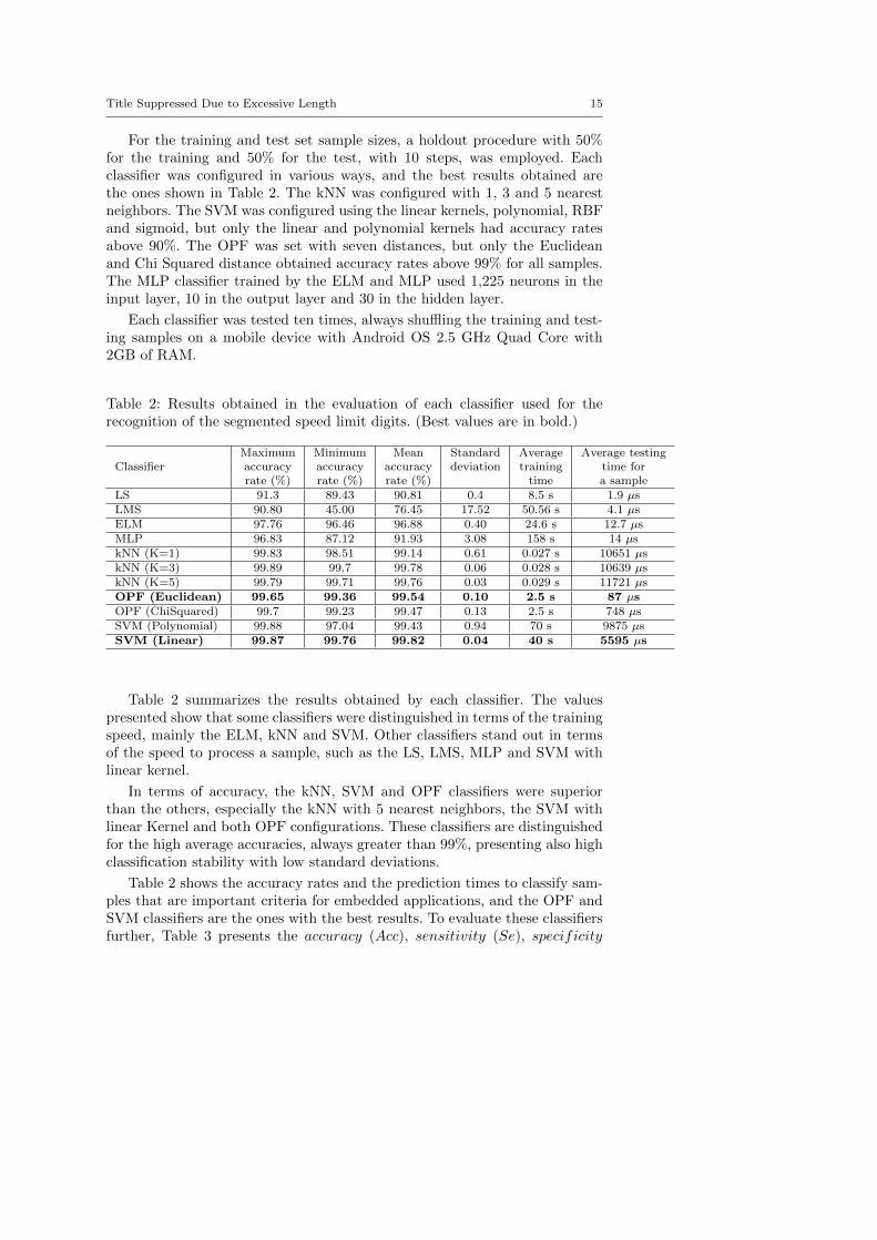
For the training and test set sample sizes, a holdout procedure with 50%for the training and 50% for the test, with 10 steps, was employed. Eachclassifier was configured in various ways, and the best results obtained arethe ones shown in Table 2. The kNN was configured with 1, 3 and 5 nearestneighbors. The SVM was configured using the linear kernels, polynomial, RBFand sigmoid, but only the linear and polynomial kernels had accuracy ratesabove 90%. The OPF was set with seven distances, but only the Euclideanand Chi Squared distance obtained accuracy rates above 99% for all samples.The MLP classifier trained by the ELM and MLP used 1,225 neurons in theinput layer, 10 in the output layer and 30 in the hidden layer.

Each classifier was tested ten times, always shuffling the training and test-ing samples on a mobile device with Android OS 2.5 GHz Quad Core with2GB of RAM.

Table 2: Results obtained in the evaluation of each classifier used for therecognition of the segmented speed limit digits. (Best values are in bold.)

Maximum Minimum Mean Standard Average Average testingClassifier accuracy accuracy accuracy deviation training time for

rate (%) rate (%) rate (%) time a sampleLS 91.3 89.43 90.81 0.4 8.5 s 1.9 µsLMS 90.80 45.00 76.45 17.52 50.56 s 4.1 µsELM 97.76 96.46 96.88 0.40 24.6 s 12.7 µsMLP 96.83 87.12 91.93 3.08 158 s 14 µskNN (K=1) 99.83 98.51 99.14 0.61 0.027 s 10651 µskNN (K=3) 99.89 99.7 99.78 0.06 0.028 s 10639 µskNN (K=5) 99.79 99.71 99.76 0.03 0.029 s 11721 µsOPF (Euclidean) 99.65 99.36 99.54 0.10 2.5 s 87 µsOPF (ChiSquared) 99.7 99.23 99.47 0.13 2.5 s 748 µsSVM (Polynomial) 99.88 97.04 99.43 0.94 70 s 9875 µsSVM (Linear) 99.87 99.76 99.82 0.04 40 s 5595 µs

Table 2 summarizes the results obtained by each classifier. The valuespresented show that some classifiers were distinguished in terms of the trainingspeed, mainly the ELM, kNN and SVM. Other classifiers stand out in termsof the speed to process a sample, such as the LS, LMS, MLP and SVM withlinear kernel.

In terms of accuracy, the kNN, SVM and OPF classifiers were superiorthan the others, especially the kNN with 5 nearest neighbors, the SVM withlinear Kernel and both OPF configurations. These classifiers are distinguishedfor the high average accuracies, always greater than 99%, presenting also highclassification stability with low standard deviations.

Table 2 shows the accuracy rates and the prediction times to classify sam-ples that are important criteria for embedded applications, and the OPF andSVM classifiers are the ones with the best results. To evaluate these classifiersfurther, Table 3 presents the accuracy (Acc), sensitivity (Se), specificity


Table 3: Acc, Se, Sp, FS for the worst case of the SVM, with linear andpolynomial kernel, and OPF, with Euclidean and Chi Squared distances.

SVM

Linear kernel Polynomial kernelclass Sp(%) Se(%) HM(%) Acc(%) class Sp(%) Se(%) HM(%) Acc(%)

0 99.94 100.0 99.95 99.72 0 99.97 100.0 99.97 99.861 99.96 100.0 99.96 99.83 1 100.0 74.04 97.18 85.092 99.97 100.0 99.97 99.89 2 100.0 100.0 100.0 100.03 100.0 99.17 99.91 99.58 3 96.87 99.88 97.17 87.534 99.94 99.78 99.92 99.67 4 100.0 99.78 99.97 99.895 99.98 100.0 99.98 99.93 5 99.96 100.0 99.96 99.806 99.98 99.76 99.96 99.82 6 100.0 99.53 99.95 99.767 99.97 99.85 99.96 99.78 7 99.98 99.85 99.97 99.858 99.97 99.51 99.92 99.63 8 99.97 99.63 99.94 99.699 99.98 99.59 99.94 99.74 9 99.94 99.89 99.94 99.74

Total 99.97 99.76 99.95 99.76 Total 99.67 97.04 99.40 97.04

OPF

Euclidean Distance Chi Squared Distanceclass Sp(%) Se(%) HM(%) Acc(%) class Sp(%) Se(%) HM(%) Acc(%)

0 99.93 100.0 99.94 99.71 0 99.97 99.81 99.96 99.811 99.95 100.0 99.96 99.80 1 99.97 99.81 99.96 99.812 99.61 100.0 99.65 98.37 2 99.95 99.81 99.94 99.723 99.95 96.48 99.61 98.02 3 99.97 98.97 99.87 99.394 100.0 99.64 99.96 99.82 4 99.93 99.81 99.92 99.625 100.0 99.81 99.98 99.90 5 99.91 99.62 99.89 99.446 99.95 98.91 99.85 99.27 6 99.65 99.08 99.60 98.007 99.97 99.82 99.96 99.82 7 99.97 100.0 99.98 99.918 99.91 99.07 99.83 99.16 8 99.79 96.51 99.47 97.319 99.95 99.82 99.94 99.73 9 99.95 98.89 99.85 99.25

Total 99.92 99.36 99.87 99.36 Total 99.91 99.23 99.84 99.23

(Sp) and Harmonicmeans (HM) metrics for each class under study for theworst case obtained.

The values presented in Table 2 show that the SVM with linear Kernelstands out as it has the highest accuracy and lowest standard deviation. Also,OPF with Euclidean distance had the lowest test time compared to the otherclassifiers; its training time was 16 times lower and the testing time was 64times lower than the SVM with linear kernel. The OPF with Euclidean dis-tance had an average accuracy of 99.54±0.10.

These findings confirm that the OPF classifier with Euclidian distanceis suitable to be integrated in an android application for speed limit signrecognition with high efficiency.

The standardized digit sizes obtained in the DIP step, and used in theclassifiers evaluation for the pattern recognition step are available at website

http://lapisco.ifce.edu.br/?page_id=140


5.3 Overall results and main contributions

Many methods have been proposed to detect speed signs, often using somereference object in the input images. The first contribution of the frameworkproposed is the detection of speed signs based on a cascade of boosted clas-sifiers combined with haar-like features. This approach detects speed signsindependent of the image acquisition distance, which is an important featuresince the signs are smaller the further they are from the camera. This is becausesamples of signs with various sizes were used in the training of the cascadeclassifier.

Another important contribution of the proposed framework is not havingto use additional attributes, since the digits are resized to a standard sizeof 35x35 pixels. By doing this, it was found that the digits are invariant interms of size, but here this is attained by processing the image and not inthe recognition step as is normally done. This increases the recognition speedand robustness. Another contribution is also related to the processing speed,verifying seven types of classifiers to check which one had the best recognitionperformance and low processing time. The top recognition rate obtained wassuperior to 99.7% with the SVM and OPF classifiers performing in real timein the embedded system.

Analyzing the framework in an optimal configuration, we obtained a de-tection and recognition of 89.19%, which corresponds to 11,167 signs correctlydetected and recognized from a database with 12,520 signs. The speed of theembedded system varied between 20 and 30 frames per second, depending onthe number of signs found in the input image.

All the solutions that were developed here are fast and able to be embeddedin commercial systems.

The drawback of the methodology developed is the error generated bylarge rotations, but this can be mitigated with the correct configuration of thecamera.

6 Conclusion

The addresed problem is very challenging because with the growth of citiesand the rise in the number of cars on the streets, it is extremely important touse systems able to identifying speed limit signs.

The objectives defined for this work were fully met, since the system de-veloped is able to detect and recognize the speed limit signs satisfactorily. Thedeveloped system successfully segmented the speed signs and recognized theirvalues with high accuracy.

The system obtained a global detection and recognition rate of 89.19%,with 90.41% in the detection step and 98.64% in the recognition step. Fromthe images tested, it can be concluded that the system implemented is quitetolerant relative to the size of the image to be evaluated.


Even with good results, this work has some limitations. First, the systemimplemented is limited in terms of the distance between the image device andthe speed limit sign, and the rotation involved, since when these are high, theidentification can be erroneous.

Acknowledgements

Pedro Pedrosa Reboucas Filho acknowledges the sponsorship from the Insti-tuto Federal do Ceara (IFCE) via grants PROINFRA/2013, PROAPP/2014and PROINFRA/2015. Victor Hugo C. Albuquerque acknowledges the spon-sorship from the Brazilian National Council for Research and Development(CNPq) through grants 470501/2013-8 and 301928/2014-2.

Authors gratefully acknowledge the funding of Project NORTE-01-0145-FEDER- 000022 - SciTech - Science and Technology for Competitive andSustainable Industries, co-financed by Programa “Operacional Regional doNorte (NORTE2020)”, through “Fundo Europeu de Desenvolvimento Regional(FEDER)”.

References

1. S.L. Gomes, E.S. Reboucas, P.P. Reboucas Filho, Revista SODEBRAS 9,9 (2014)

2. E.C. Neto, S.L. Gomes, P.P.R. Filho, V.H.C. de Albuquerque, Measure-ment 70, 36 (2015)

3. C. Tu, B. van Wyk, Y. Hamam, K. Djouani, S. Du, in International Con-ference on Electronic Engineering and Computer Science (EECS 2013),vol. 4 (2013), vol. 4, pp. 316 – 322

4. S.C. Yi, Y.C. Chen, C.H. Chang, Computers and Electrical Engineering42, 23 (2015)

5. S. Yu, Z. Shi, Physica A: Statistical Mechanics and its Applications 428,206 (2015)

6. S. Carrese, S. Mantovani, M. Nigro, Transportation Research Part E: Lo-gistics and Transportation Review 65(0), 35 (2014)

7. B.F. Wu, H.Y. Huang, C.J. Chen, Y.H. Chen, C.W. Chang, Y.L. Chen,Computers and Electrical Engineering 39(3), 846 (2013)

8. I. Garcia, S. Bronte, L. Bergasa, J. Almazan, J. Yebes, in Intelligent Ve-hicles Symposium (IV) (2012), pp. 618–623

9. J.P.A. Barthes, P. Bonnifait, in Advances in Artificial Transportation Sys-tems and Simulation (Academic Press, Boston, 2015), pp. 163 – 180

10. P. Viola, M. Jones, in IEEE Computer Society Conference on ComputerVision and Pattern Recognition, vol. 1 (2001), vol. 1, pp. 511–518

11. R. Lienhart, J. Maydt, in International Conference on Image Processing,vol. 1 (2002), vol. 1, pp. I–900–I–903 vol.1


12. M. Rezaei, H. Ziaei Nafchi, S. Morales, in Image and Video Technology,Lecture Notes in Computer Science, vol. 8333 (Springer Berlin Heidelberg,2014), Lecture Notes in Computer Science, vol. 8333, pp. 302–313

13. P. Elmer, A. Lupp, S. Sprenger, R. Thaler, A. Uhl, in Image Analysis,Lecture Notes in Computer Science, vol. 9127, ed. by R.R. Paulsen, K.S.Pedersen (Springer International Publishing, 2015), Lecture Notes in Com-puter Science, vol. 9127, pp. 53–64

14. A.P. Mena, M. Bachiller Mayoral, E. Dıaz-Lope, in Bioinspired Computa-tion in Artificial Systems, Lecture Notes in Computer Science, vol. 9108(Springer International Publishing, 2015), Lecture Notes in Computer Sci-ence, vol. 9108, pp. 175–183

15. G. Rakate, S. Borhade, P. Jadhav, M. Shah, in IEEE International Confer-ence on Computational Intelligence Computing Research (ICCIC) (2012),pp. 1–5

16. S. Zhang, C. Bauckhage, A. Cremers, in IEEE Conference on ComputerVision and Pattern Recognition (CVPR) (2014), pp. 947–954

17. K. Zheng, Y. Zhao, J. Gu, Q. Hu, in IEEE International Symposium onIndustrial Electronics (ISIE) (2012), pp. 1502–1505

18. F. Amat, P. Keller, in 10th International Symposium on Biomedical Imag-ing (ISBI) (2013), pp. 1194–1197

19. J.H. da Silva Felix, P.C. Cortez, P.P. Reboucas Filho, A.R. de Alexan-dria, R.C.S. Costa, M.A. Holanda, in MICAI 2008: Advances in ArtificialIntelligence (Springer, 2008), pp. 957–964

20. P.P. Reboucas Filho, P.C. Cortez, J.H.d.S. Felix, T.d.S. Cavalcante, M.A.Holanda, Revista Brasileira de Engenharia Biomedica 29(4), 363 (2013)

21. J. Canny, IEEE Transactions on Pattern Analysis and Machine Intelli-gence (6), 679 (1986)

22. J.M.R. Tavares, P.P. Reboucas Filho, T.D.S. Cavalcante, V.H.C. de Al-buquerque, Journal of Testing and Evaluation 38(1), 1 (2009)

23. A. McAndrew, Introduction do digital image processing with matlab(Thomson Learning, 2004)

24. V.H.C. Albuquerque, P.P. Reboucas Filho, T. da Silveira Cavalcanti,J.M.R.S. Tavares, Journal of Microscopy 240(1), 50 (2010)

25. P.P. Reboucas Filho, P.C. Cortez, A.C. da Silva Barros, V.H.C. Albu-querque, Expert Systems with Applications 41(17), 7707 (2014)

26. P.P. Reboucas Filho, F.D.L. Moreira, F.G. de Lima Xavier, S.L. Gomes,J.C. Santos, F.N.C. Freitas, R.G. Freitas, Materials 8(7), 3864 (2015)

27. F.D.L. Moreira, M.N. Kleinberg, H.F. Arruda, F.N.C. Freitas, M.M.V.Parente, V.H.C. de Albuquerque, P.P. Reboucas Filho, Expert Systemswith Applications 45, 294 (2016)

28. R.O. Duda, P.E. Hart, Communications of the ACM 15(1), 11 (1972)29. H.K. Yuen, J. Illingworth, J. Kittler, Image and Vision Computing 7(1),

31 (1989)30. E.C. Neto, E.S. Reboucas, J.L. Moraes, S.L. Gomes, P.P. Reboucas Filho,

IEEE Transactions on Latin America 13, 272 (2015)31. B. Scholkopf, A.J. Smola, Learning with Kernels (MIT Press, 2002)


32. V.N. Vapnik, IEEE Transactions on Neural Networks 10(5), 988 (1999)33. C. Cortes, V. Vapnik, Machine Learning 20(3), 273 (1995)34. C. Burges, Data Mining and Knowledge Discovery 2(2), 121 (1998)35. C.C. Chang, C.J. Lin, ACM Trans. Intell. Syst. Technol. 2(3), 27:1 (2011)36. J.P. Papa, A.X. Falcao, C.T.N. Suzuki, International Journal of Imaging

Systems and Technology 19(2), 120 (2009)37. J.P. Papa, A.X. Falcao, V.H.C. de Albuquerque, J.M.R.S. Tavares, Pattern

Recognition 45(1), 512 (2012)38. A.X. Falcao, J. Stolfi, R.A. Lotufo, IEEE Transactions on Pattern Analysis

and Machine Intelligence 26(1), 19 (2004)39. J.P. Papa, A.X. Falcao, C.T. Suzuki, International Journal of Imaging

Systems and Technology 19(2), 120 (2009)40. V.H.C. Albuquerque, C.V. Barbosa, C.C. Silva, E.P. Moura, P.P. Re-

boucas Filho, J.P. Papa, J.M.R.S. Tavares, Sensors 15(6), 12474 (2015)41. J.A. Plucker, A. Esping. Human intelligence: Historical influences,

current controversies, teaching resources. (2016). URL http://www.

intelltheory.com

42. G. Bittencourt, Artificial Intelligence - Tools and Theories, 3rd edn. (Fed-eral University of Santa Catarina, 2006)

43. T. Kohonen, Self-organization and associative memory: 3rd edition(Springer-Verlag New York, Inc., New York, NY, USA, 1989)

44. O. Helene, Method of least squares (Livraria da Fısica, 2006)45. S.O. Haykin, Neural Networks and Learning Machines (Pearson Prentice

Hall, 2008)46. B. Widrow, Proceedings of the IEEE 78, 1415 (1990)47. B. Widrow, R. Winter, IEEE Computer 21, 25 (1988)48. P. Horata, S. Chiewchanwattana, K. Sunat, Neurocomputing 102, 31

(2013)49. A.L.B.P. Barros, G.A. Barreto, in Brazilian Conference on Intelligent Sys-

tems (Curitiba, PR, Brasil, 2012)50. G.B. Huang, D.H. Wang, Y. Lan, International Journal of Machine Learn-

ing and Cybernetics 2, 107 (2011)51. G.B. Huang, Q.Y. Zhu, C.K. Siew, Neurocomputing 70, 489 (2006)52. G.B. Huang, L. Chen, C.K. Siew, IEEE Transactions on Neural Networks

17, 879 (2006)53. D.W. Ruck, S.K. Rogers, M. Kabrisky, M.E. Oxley, B.W. Suter, IEEE

Transactions on Neural Networks 1(4), 296 (1990)54. S. Nissen, Implementation of a Fast Artificial Neural Network Library

(FANN) (2003). Department of Computer Science University of Copen-hagen (DIKU).

55. M. Minsky, S. Papert, Perceptrons (M.I.T Press, 1969)56. F.M. de Azevedo, L.M. Brasil, R.C.L. de Oliveira, Neural networks with

applications Control and Expert Systems (Visual Books, 2000)57. C. Medeiros, G. Barreto, Neural Computing and Applications 22(1), 71

(2013)

http://www.intelltheory.com

http://www.intelltheory.com


58. M.A. Arbib, The handbook of Brain Theory and Neural Networks (M.I.TPress, 2003)

59. G. Barreto, R. Frota, Pattern Analysis and Applications 16(1), 83 (2013)60. S.J. Russell, P. Norvig, Artificial Intelligence: A Modern Approach (3rd

Edition) (Prentice-Hall, 2009)61. H.E. Kocer, K.K. Cevik, Procedia Computer Science 3, 1033 (2011)62. W. Schimidt, IEEE International Conference on Neural Networks 1, 598

(1993)63. M. Riedmiller, H. Braun, in IEEE International Conference on Neural

Networks (1993), pp. 586–591 vol.164. C.A. Glasbey, CVGIP: Graphical Models and Image Processing 55, 532

(1993)

Documents

Embedded real time speed limit sign recognition using ...tavares/downloads/publications/artigos/NCAA... · Embedded real time speed limit sign recognition using image processing and