Embed Size (px)
Citation preview

EM Section 4: Electrostatic Energy
Energy has not been mentioned much in the course thus far. This section defines electrical potential,
potential difference and potential energy. The fundamental link between the electric field and electric
potential is established, and from there it is shown how some of the field results could have been derived
using potentials, in possibly a simpler way as vector components need not be considered. The importance
of the electrostatic field as a conservative force field is emphasised, and from this some of the
fundamental results of vector calculus as applied to such fields are consolidated.
4.1 Electrical potential difference
Consider a test charge 𝑞 that moves from a point 𝐴 to a point 𝐵 in an electrostatic field 𝑬. If the force
on the charge due to the electric field is 𝑭 then the total work required to move the charge is given by
𝑊𝐴→𝐵 = −∫ 𝑭 ∙ 𝑑𝒔𝐵
𝐴 where 𝑑𝒔 is the infinitesimal vector displacement along the path.
The minus sign is necessary as this is the force required to work required to move the charge. The
expression for the work done on the charge by the field during the journey is simply +∫ 𝑭 ∙ 𝑑𝒔𝐵
𝐴.
This quantity will vary depending on the size of the charge in question. But if the work per unit charge is
considered a more important quantity emerges. As the force at any point is given by 𝑞𝑬 the work
supplied per unit charge is given by 𝑊𝐴→𝐵
𝑞= − ∫ 𝑬 ∙ 𝑑𝒔
𝐵
𝐴 and this quantity is a property of the
electrostatic field alone. This quantity is defined as the electrical potential difference, 𝑉𝐴→𝐵 due to the field
and thus given by
𝑉𝐴→𝐵 = −∫ 𝑬 ∙ 𝑑𝒔𝐵
𝐴 Equation 4.1
This is often more simply referred to as the potential difference (PD) between the two points. Potential
difference is a scalar quantity with SI units of JC−1 or volts (V), and with SI base units of
kg.m2. s−3. A−1. Of course, you have met the volt long ago in the context of circuits and Ohm’s law,
usually expressed in equation form as 𝑉 = 𝐼𝑅; the definition of one volt is actually in terms of circuits –
one volt is the difference in potential between two points that drives a current of one ampere through a
resistance of one ohm.
For a uniform electric field equation 4.1 simplifies to 𝑉𝐴→𝐵 = −𝑬.𝒅 where 𝑑 is the displacement from
𝐴 to 𝐵.
The potential difference between ground level and 10 m up on the Earth (field strength 100 NC−1
downwards) would be about +1,000 V. This means to move a +1 C charge from ground to 10 m of
altitude requires about +1,000 J of energy.

Conversely the potential difference between 10 m up and ground level is about −1,000 V and moving
+1 C from 10 m to ground requires about= 1,000 J.
Let us re-emphasise that the potential difference between two points is a property of the electric field
itself and has nothing to do with the charges present in the field; the PD between two points is always
there whether or not a charge wants to move between them.
A semantic point on potential difference and volts
Potential difference has SI units of volts. This has lead to a common usage of the term “voltage” in
speech to describe PD. While this is so commonplace that it almost universally accepted you should try
not to use the term voltage in discourses related to electromagnetism. Potential difference is the quantity
and the volt is the unit. Saying “voltage” is like using “jouleage” for energy or “newtonage” for force. As
well as being (too) informal it also removes a little bit of meaning from the terminology as it the term
voltage is often applied to a point or a thing (like a battery), whereas what is essential about potential
difference is that is related to the difference in something between two points.
More on uniform fields
Consider a uniform electric field between two parallel uniformly charged plates separated by a distance
𝑑. The field has magnitude 𝐸 and the potential difference between the plates is 𝑉.
If a charge is placed in the field, the force on the charge is given by 𝐸𝑞 and the work done in moving
the charge a distance 𝑑 is thus given by 𝐸𝑞𝑑 by definition.
But now using the definition of potential difference, the magnitude of the work done in moving the
charge the distance 𝑑 can also be given by 𝑞𝑉.
Equating these two terms gives 𝐸𝑞𝑑 = 𝑞𝑉 and thus the magnitude of the electric field strength between
the plates can be expressed by
𝐸 =𝑉
𝑑 Equation 4.2
which is a widely used formula for uniform field strengths. This shows that an alternative unit for
electric field strength is the Vm−1.
There is no absolute potential
Just as gravitational potential energy always must be defined relative to some reference point, so must
electric potential energy. This is why is absolutely necessary to refer to the potential difference between to

points. To simply state that one point has a potential difference is meaningless – it must be given relative
to another point in the field.
That said, as with gravitational potentials, it is sometimes convenient to define the zero of potential as
being at an infinite distance from the sources of the field; this is done now when considering the potential
due to a point charge.
4.2 Binding energy and the potential due to a point charge
The electric potential, 𝑉 at a point at distance 𝑟 from a point charge 𝑄 is defined as the work done per
unit charge in bringing another object from infinity to the point. For a point charge the equation for
electric potential is given by
𝑉 =1
4𝜋𝜖0
𝑄
𝑟 Equation 4.3
The potential at a distance of 1 cm from a point charge of +1 C is therefore about +900 GJC−1. This
means that if another charge of +1 C is brought from a large distance away to within 1 cm of the charge
then it will need +900 GJ of work to be done on it. Or the other way round, if the charges were placed
1 cm apart and one was held stationary the other would gain 900 GJ when repelled. In the absence of the
friction the work-energy theorem means that that this will be entirely kinetic energy.
Proof of equation 4.3
Consider a test charge 𝑞 that is initially a distance 𝑟 along the 𝑥-axis from a charge 𝑄 that is fixed in
position. Let’s calculate how much work is needed to carry the test charge away to an infinite distance
from 𝑄:
The test charge is carried away at a constant speed so its kinetic energy does not increase - the
electrostatic force of attraction or repulsion on the charge 𝑞 is thus exactly balanced by the contact force
supplied by the agent carrying the it away:
Figure 4.1 A test charge being carried a long distance away from 𝒓

The work done in moving the test charge a small displacement 𝛿𝑥 is given by 𝛿𝑊 = 𝐹. 𝛿𝑥 where 𝐹 is
the force on the test charge and 𝛿𝑥 the infinitesimal displacement that it moves. When a distance 𝑥 away
this force will be −1
4𝜋𝜖0
𝑄𝑞
𝑥2 as it acts left to right (positive in the system sketched above).
This gives
𝛿𝑊 = (−1
4𝜋𝜖0
𝑄𝑞
𝑥2) ∙ (𝛿𝑥) = −1
4𝜋𝜖0
𝑄𝑞
𝑥2 ∙ 𝛿𝑥
So the total work done on moving from 𝑟 to infinity is given by
𝑊 = −1
4𝜋𝜖0𝑄𝑞 ∫
𝑑𝑥
𝑥2
𝑥=∞
𝑥=𝑟
= −1
4𝜋𝜖0
𝑄𝑞
𝑟
This is the known as the binding energy of two charges separated by a distance 𝑟 and is the amount of
energy required to separate them far enough so that their mutual electrostatic force of attraction is
negligible. Note that this is negative for like charges, and positive for unlike charges (as it should be).
The potential energy, 𝑈, of the two objects is given by the negative of the binding energy - it is the
amount of work required to bring the two objects from infinite separation to a separation 𝑟.
To state this generally for two charges 𝑄1 and 𝑄2 the electrical potential energy is given by
𝑈 =1
4𝜋𝜖0
𝑄1𝑄2
𝑟 Equation 4.4
The electrostatic potential energy per unit charge of an object is hence given by equation 4.3.
Also note the potential energy does not belong to one object nor the other, rather it is shared between
the two objects (or can be said to be a property of the system).
Charges move so as to minimise their shared potential energy
We often elucidate the movement of charges by seeing which direction the vector force field pushes the
charge in. Another way to decide which way a charge will move is by realising that it will always move to
minimise its shared electrical potential energy between itself and whatever other charges are in its vicinity.
For unlike charges this means moving together so 𝑈 → −∞ by equation 4.4 and for like charges this
means moving apart so 𝑈 → 0.
4.3 Equipotentials
In addition to electric field lines, lines of constant potential – equipotentials – are useful additions to
sketches when understanding the physics of electrostatic situations. Equipotential lines are always

perpendicular to field lines. For a uniform field they are parallel lines that run perpendicular to the field
lines, and for point charges they are concentric circles surrounding the charge. The latter is corroborated
by equation 4.3 which specifies that the potential is constant at a fixed distance from the sphere.
Several equipotential line sketches are shown in figure 4.2

Figure 4.2 Several equipotential line sketches; the equipotential lines are represented with a dashed line.
Note they always cross perpendicular to the field lines.
If a charge moves along an equipotential then its electrostatic potential energy stays constant. This is
further explored in the next section.
4.4 The electrostatic field as a conservative field
We are now in a position to ruminate on the equations of electrostatics with a greater level of maturity
than ever before:
The vector electrostatic field is the gradient of the scalar electric potential field
Equation 4.1 defines the potential difference between two point in an electric field in terms of a path
integral over a section of the electric field; an equivalent way of writing this equation – writing the field as
the subject of the formula is to say
𝑬 = −∇𝑉 Equation 4.5

Although equations 4.1 and 4.5 are essentially equivalent – neither contains any information that the
other doesn’t – we can now appreciate electrostatics from a new point of view: if a system of stationary
charges exist then they produce a scalar potential field, and a vector electric field throughout all space.
Provided one point is (arbitrarily) defined as the zero of potential then equation 4.1 and 4.5 can be used
to completely define one using the other.
The curl of the electrostatic field is zero
Equation 4.5 can be used to quickly demonstrate that the curl of the electrostatic field is zero. Taking
the curl of both side of equation 4.5 gives ∇ × 𝑬 = −∇ × (∇𝑉⃗⃗⃗⃗ ⃗) . From the definition of gradient,
divergence and curl it is easy to prove (see your vector calculus notes) that the curl of the gradient of any
scalar field is zero, hence
∇ × 𝑬 = 0 Equation 4.6
A handwaving interpretation of this result is that if there were a light, electrically charged paddlewheel
placed in a electrostatic field then no arrangement of charges could cause the paddlewheel to turn. A
simplified corollary of the result is that the electrostatic field due to a point charge is spherically
symmetric.
The work done in moving a charge around a closed path in an electrostatic field is zero
Stokes theorem can be used to derive this rule. The form of Stokes theorem that most closely aligns
with the mathematical setup we are using states that the surface integral of the curl of a vector field
enclosing a surface equals the closed loop path integral of the vector field over its boundary. i.e.
∬∇ × 𝑬
𝑆
. 𝑑𝑆 = ∮ 𝑬. 𝑑𝒓
𝐶
As the curl of the field is zero this shows that the ∮ 𝑬. 𝑑𝒓𝐶
= 0 and as the field is directly proportional
to the force on a test charge it can be stated that
∮ 𝑭. 𝑑𝒓𝐶
= 0 Equation 4.7
which means that the total work done in moving in any closed loop in any electrostatic field is zero.
Path independence
It follows from this result that the work done in moving from one point to another point in an
electrostatic field is independent of path – if it varied depending on the path then in would be possible to
pick up extra energy on closed route depending on the route thus contradicting the above.
Conservative fields
These three rules: (i) that the electric field is the gradient of a scalar potential field, (ii) that the curl of the
vector field is zero and (iii) that the work done in a closed loop is path independent are all properties of
what are known as conservative fields in mathematics and physics. Essentially they are all fields where
mechanical energy is conserved when moving within the field i.e. when an object moves within the field
the sum of its kinetic energy and potential energy due to its position within the field is constant at all
times.
Any one of these conditions implies the other two. It is mathematically impossible for one to be correct
without the other two being so, hence when stating a field is conservative if suffices to state one of the
conditions hold alone and the other two may be inferred without further ado.
Conservative fields exist when the force on a body in the field can be computed as a function of its
position alone. If a force field exists where the force on a body is function of something else (such as time
or velocity) then the force will not be conservative. And just as if one of the conditions for conservative
force fields is true then the other two must be, the opposing statement also holds viz. if one of the
conditions is not met for a force field, then the other two cannot be true.
e.g. consider a frictional force arising when sliding a book on a table. It is clear that the work done
needed to push it from one point to another depends on the route taken, and also that the work done
going in a closed loop is non-zero hence it is not conservative. The force cannot be described simply as a
function of position, nor is mechanical energy conserved in its movement.
Electrostatics is conservative forces plus the inverse square law
From the chapter on Gauss’s law we know that the divergence of an electrostatic field is directly
proportional to the charge enclosed in the field and in fact
∇. 𝑬 =𝜌
𝜖0 Equation 3.4
And now we know further that the electric field can be expressed as the gradient of a scalar potential
field so combining this with equation 4.5 we get
∇2𝑉 = −𝜌
𝜖0 Equation 4.8
which is simply another way of stating Gauss’s law for electrostatics.
4.8 essentially summarises all of electrostatics: it implies the force field is conservative, and that it is an
inverse square relation.
Incidentally, 4.8 is a type of equation known as Poisson’s equation and it is an important second order
partial differential equation. Methods of finding solutions to Poisson’s equation are taught in year 2.
4.5 Calculations using potential instead of force
For any arrangement of charges, either discrete or continuous, it is always to compute the electric field
strength at a point using Coulomb’s law and the principle of superposition. If the arrangement of charges
can be mathematically defined them it may be possible to derive an exact mathematical expression for the
field, else a numerical approximation may be produced instead. One of the difficulties with doing this can
be in the resolution of components of the field. In 𝑁 dimensions there are always 𝑁 components to
consider and this can lead to fiddly mathematics.
The use of potentials can make life easier. Calculating the potential at a point also uses the principle of
superposition for each point charge but doesn’t require resolution of components. Use of 𝑬 = −∇𝑉 can
then give the electric field.
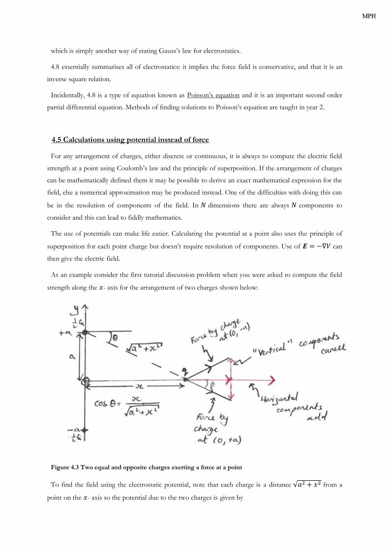
As an example consider the first tutorial discussion problem when you were asked to compute the field
strength along the 𝑥- axis for the arrangement of two charges shown below:
Figure 4.3 Two equal and opposite charges exerting a force at a point
To find the field using the electrostatic potential, note that each charge is a distance √𝑎2 + 𝑥2 from a
point on the 𝑥- axis so the potential due to the two charges is given by

2 ×1
4𝜋𝜖0
1
2𝑄
√𝑎2 + 𝑥2=
1
4𝜋𝜖0
𝑄
√𝑎2 + 𝑥2
So to find the field,
𝑬 = −∇𝑉 = −(�̂�𝜕𝑉
𝜕𝑥+ �̂�
𝜕𝑉
𝜕𝑦+ �̂�
𝜕𝑉
𝜕𝑧)
and noting that the potential only has an 𝑥- dependence this simplifies to
𝑬 = −�̂�𝜕
𝜕𝑥(
1
4𝜋𝜖0
𝑄
√𝑎2 + 𝑥2) =
1
4𝜋𝜖0
𝑄𝑥
(𝑎2 + 𝑥2)3
2⁄�̂�
which is the same result as obtained before but through less fiddly mathematics.