Embed Size (px)
Citation preview

Elsevier Editorial System(tm) for Journal of Hydrodynamics, Ser. B Manuscript Draft Manuscript Number: HYDROD-D-15-00036R2 Title: Numerical Study of Roll Motion of a 2-D floating structure in viscous flow Article Type: Original Article Keywords: OpenFOAM; CFD; Potential flow theory; Roll motion; 2-D floating structure; Regular waves; Wave forces; Viscous flow Corresponding Author: Ms. Lifen CHEN, Corresponding Author's Institution: Dalian University of Techonology First Author: Lifen CHEN Order of Authors: Lifen CHEN; Liang Sun; Jun Zang; Andrew J Hillis; Andrew R Plummer Abstract: In the present study, an open source CFD tool, OpenFOAM has been extended and applied to investigate roll motion of a 2-D rectangular barge induced by nonlinear regular waves in viscous flow. Comparisons among the present OpenFOAM results with published potential-flow solutions and experimental data have indicated that the newly extended OpenFOAM model is very capable of accurate modelling of wave interaction with freely rolling structures. The wave-induced roll motions, hydrodynamic forces on the barge, velocities and vorticity flow fields in the vicinity of the structure in the presence of waves have been investigated to reveal the real physics involved in the wave induced roll motion of a 2-D floating structure. Parametric analysis has been carried out to examine the effect of structure dimension and body draft on the roll motion. Suggested Reviewers: Dezhi Ning [email protected] He is famous for numerical modelling of wave-current interactions FuPing Gao [email protected] He is expert in wave hydrodynamics WenYang Duan [email protected] He is expert in both numerical modelling and hydrodynamic performance of floating objects in waves. Response to Reviewers: Reviewer #3: Addressing comment #2, the authors have "\Delta z is a small parameter specifying the depth of the free surface." This is confusing and it is better to use "the width of the air-water interface" or a similar term. Revised as suggested. See page 5.

The answer to comment #3: "The moments are calculated by summing the moments about COG over the body surface due to the pressure obtained by solving Navier- Stokes equations, Eqn. (1) and Eqn. (8). The viscous effect is taken into account in N-S equations which means that the viscous effect is considered in Eqn. (10). The viscous force in OpenFoam is defined as the viscous stress in the turbulent boundary layer. In the present numerical simulation, the laminar model is used. So there is no viscous force." This is incorrect. The viscous effect is taken into account in N-S equations, which DOES NOT mean that the viscous effect is automatically considered in Eqn. (10). Even for a laminar model, the moments due to the viscous stresses should be included in M before you claim that the viscous effect is considered in Eqn. (10). Unless the molecular viscosity in your model is zero, there IS viscous force. The authors apologize for the lack of clarity in this paragraph, as the laminar flow model was used in this study, similar to de Bruijn et al. (2011), we thought the viscous force may not be significant compared with other forces. Following reviewer’s comments, we have revised the text in the paper, a new reference is also added. See page 6-7. Apart from above changes, we have also made some minor changes to the paper to improve the quality of the paper. Reference: R. de Bruijun, F. Huijs, R. Huijsmans, T. Bunnik, M. Gerritsma, Calculation of wave forces and internal loads on a semi-submersible at shallow draft using an IVOF method. Proceedings of the ASME 2011 30th International Conference on Ocean, Offshore and Arctic Engineering,Rotterdam, The Netherlands, 2011.

22 June 2015
Dear Editor,
The manuscript titled “Numerical Study of Roll Motion of a 2-D floating structure in viscous
flow” has been revised according to the suggestions provided by the reviewers. Every
comment has been answered and the manuscript has been updated, with modified text
highlighted in red.
The anonymous reviewers are greatly acknowledged for their comments and their
contribution in the improvement of the manuscript. Every comment from the reviewers has
been carefully addressed, with detailed answers provided. My co-authors and I now look
forward to the publication of our work in Journal of Hydrodynamics.
Sincerely yours,
Lifen Chen,
PhD student
WEIR Research Unit
Department of Architecture and Civil Engineering,
University of Bath,
UK
Email: [email protected] or ([email protected])
Cover Letter

Reviewer #3:
Addressing comment #2, the authors have "\Delta z is a small parameter specifying the depth
of the free surface." This is confusing and it is better to use "the width of the air-water
interface" or a similar term.
Revised as suggested. See page 5.
The answer to comment #3: "The moments are calculated by summing the moments about
COG over the body surface due to the pressure obtained by solving Navier- Stokes equations,
Eqn. (1) and Eqn. (8). The viscous effect is taken into account in N-S equations which means
that the viscous effect is considered in Eqn. (10). The viscous force in OpenFoam is defined
as the viscous stress in the turbulent boundary layer. In the present numerical simulation, the
laminar model is used. So there is no viscous force."
This is incorrect. The viscous effect is taken into account in N-S equations, which DOES
NOT mean that the viscous effect is automatically considered in Eqn. (10). Even for a
laminar model, the moments due to the viscous stresses should be included in M before you
claim that the viscous effect is considered in Eqn. (10). Unless the molecular viscosity in
your model is zero, there IS viscous force.
The authors apologize for the lack of clarity in this paragraph, as the laminar flow model was
used in this study, similar to de Bruijn et al. (2011), we thought the viscous force may not be
significant compared with other forces. Following reviewer’s comments, we have revised the
text in the paper, a new reference is also added. See page 6-7.
Apart from above changes, we have also made some minor changes to the paper to improve
the quality of the paper.
Reference:
R. de Bruijun, F. Huijs, R. Huijsmans, T. Bunnik, M. Gerritsma, Calculation of wave forces
and internal loads on a semi-submersible at shallow draft using an IVOF method.
Proceedings of the ASME 2011 30th International Conference on Ocean, Offshore and
Arctic Engineering,Rotterdam, The Netherlands, 2011.
*Detailed Response to Reviewers

*Corresponding author. Tel.: 0044 7774443761. E-mail addresses: [email protected], [email protected] (L.F. Chen), [email protected] (L.Sun), [email protected] (J. Zang), [email protected] (A.J. Hillis), [email protected] (A.R. Plummer)
Numerical Study of Roll Motion of a 2-D floating structure in
viscous flow
L.F. Chena,*
, L. Suna, J. Zang
a, A.J. Hillis
b
A.R. Plummerb
a. WEIR Research Unit, Department of Architecture and Civil Engineering, University of Bath,
BA2 7AY, UK
b. Department of Mechanical Engineering, University of Bath, Bath, BA2 7AY, UK
Abstract: In the present study, an open source CFD tool, OpenFOAM has been extended and
applied to investigate roll motion of a 2-D rectangular barge induced by nonlinear regular
waves in viscous flow. Comparisons among the present OpenFOAM results with published
potential-flow solutions and experimental data have indicated that the newly extended
OpenFOAM model is very capable of accurate modelling of wave interaction with freely
rolling structures. The wave-induced roll motions, hydrodynamic forces on the barge,
velocities and vorticity flow fields in the vicinity of the structure in the presence of waves
have been investigated to reveal the real physics involved in the wave induced roll motion of
a 2-D floating structure. Parametric analysis has been carried out to examine the effect of
structure dimension and body draft on the roll motion.
Key words: OpenFOAM; CFD; Potential flow theory; Roll motion; 2-D floating structure;
Regular waves; Wave forces; Viscous flow;
1. Introduction
The hydrodynamic motions of ships and floating structures in the presence of waves need to
be carefully examined during the early stage of structure design to ensure the stability
characteristics or energy efficiency of the structure. In reality, a ship or floating structure
experiences motion in all six degrees of freedom (DoF) simultaneously, but only roll motion
will be investigated in this paper. Roll motion is the most critical motion leading to ship or
platform capsizes compared to other five degrees of freedom motion of a ship or platform [1-
2]. The roll motion of a ship or floating structure can be determined by solving an ordinary
differential equation which contains three coefficients, the virtual mass moment of inertia for
*Manuscript

2
rolling, the damping coefficient and the restoring moment coefficient. The value of these
three coefficients can be determined experimentally or by using mathematical methods.
Among them, the damping coefficient has been considered to play the most significant role in
the roll motion calculation and should be determined accurately [3]. Model test has been one
of the most common approaches used to estimate the roll damping. Generally, the body is
rolled to a chosen angle and then released in calm water. The recorded roll time history is
used to determine the equivalent linearized roll damping by assuming that the dissipated
energy due to the nonlinear and equivalent linear damping is the same. The roll damping of
floating cylinders in a free surface was assessed by Vugts [4] experimentally. Several free-
roll model tests of ship shaped bodies and a barge-type LNG FPSO were conducted by
Himeno [5] and Choi et al. [6], respectively. Jung et al. [7-8] carried out several experiments
in a 2-D wave tank to study the roll motion of a rectangular barge. Jung et al. [8] concluded
that the roll damping in some wave conditions helps the barge to roll. Wu et al. [9] conducted
an experimental investigation to study the nonlinear roll damping of a ship in the presence of
regular and irregular waves. The recorded roll time history in calm water obtained by Wu et
al. [9] had the similar trend with that obtained by Jung et al. [8].
Physical experimentation is expensive and not always practical. Numerical methods,
including potential flow theory, empirical formula and viscous flow theory, have also been
widely used for the prediction of the roll motion. Potential flow theory like strip theory is
applied to investigate wave induced roll motion based on the assumption that the motion of a
floating structure by waves is linear. A computer program based on linear strip theory was
developed by Journée [10] for conventional mono-hull ships in their preliminary design stage.
Schmitke [11] and Lee et al. [12] used strip theory to investigate the roll damping of a ship in
beam seas and the hydrodynamic radiation damping of a rectangular barge, respectively.
Potential flow theory has been used to predict the motion of the structure in surge, heave,
pitch, sway and yaw to a reasonable degree of accuracy without any empirical correction or
recourse to experiments. However, it is found that the wave damping derived from the linear
potential flow theory is inadequate for an accurate prediction of the roll motion since the
effect of viscous damping could be as significant as those of wave damping in roll [3, 5, 13,
14].
One of the compensating methods is to introduce an artificial or empirical damping
coefficient in the computation using potential flow theory to take into account the viscous
effect. Himeno [5], Chakrabarti [13] and Ikeda et al. [15] divided the total roll damping

3
coefficient into several components, such as friction, eddy, wave damping, lift etc. Wave
damping is derived from linear potential flow theory while other components can be
computed by empirical formulas. This prediction method has been applied successfully by
inviscid-fluid models coupling with the strip theory [10, 16 – 18].
The applicability of the empirical formulas is limited by the fact that the empirical
coefficients are derived from extensive model tests or field measurements. Viscous models
based on Navier-Stokes equations are becoming increasingly popular in engineering
predictions for providing more accurate and realistic results. Yeung and Liao [19] predicted
pure heave or roll motion of a floating cylinder using a fully nonlinear model based on the
Navier-Stokes equations and found that the roll amplitude could be reduced by as much as 50%
due to the fluid viscosity. Zhao and Hu [20] developed a viscous flow solver, based on a
constrained interpolation profile (CIP)-based Cartesian grid method, to model nonlinear
interactions between extreme waves and a box-shaped floating structure, which is allowed to
heave and roll only. Bangun et al. [21] calculated hydrodynamic forces on a rolling barge
with bilge keels by solving Navier-Stokes equations based on a finite volume method in a
moving unstructured grid. The roll decay motion of a surface combatant was predicted by
Wilson et al. [22] using an unsteady Reynolds-averaged Navier-Stokes (RANS) method. The
RANS method was employed by Chen et al. [23, 24] as well to describe large amplitude ship
roll motions and barge capsizing. 2-D CFD calculations were conducted by Ledoux et al. [25]
to study the roll motion of box shape FPSOs in the west Africa fields.
OpenFOAM, an open-source CFD package, is proved to provide accurate numerical
predictions when applied to nonlinear wave interactions with fixed structures. Morgan et al.
[26, 27] has extended the OpenFOAM and reproduced the experiments on regular waves
propagation over a submerged bar successfully with up to 8th
order harmonics correctly
modelled. The extended OpenFOAM has been applied to model nonlinear wave interactions
with a vertical surface piercing cylinder and a single truncated circular column by Chen et al.
[28, 29] and Sun et al. [30], respectively. The accuracy of the models was validated by
comparing with experiments. The simulation of the prescribed angular oscillation of a 2-D
box was performed by Eslamdoost [30]. A built-in dynamic solver interDyMFoam was
extended by Ekedahl to simulate wave-induced motions of a floating structure [31]. The
model diverged after about 10 seconds for the case with a coarse mesh due to numerical
discrepancies or low mesh quality. According to Yousefi et al. [32], OpenFOAM can also be
applied to simulate the flow field around a hull, taking into account maneuverability, wave

4
and free surface effects and it is gaining increasing popularity due to its excellent
computational stability.
In this paper, the nonlinear interactions between regular waves and a 2-D rolling rectangular
barge have been studied numerically and the results are compared with the experimental
measurements collected by Jung et al. [8]. The extended OpenFOAM model developed by
Chen et al. [28; 29] is selected here for the two-phase flow modeling as well as wave
generation and absorption. Two difficulties have been solved in order to extend its capability
in simulating the roll motion of floating structures by waves: determining the wave-induced
motion of the floating structure and moving or deforming the mesh according to this motion.
The wave-induced roll motions, hydrodynamic forces on the barge, velocities and vorticity
flow fields in the vicinity of the structure in the presence of waves have been investigated in
this paper. Parametric analysis has been carried out to study the effect of the structure size
and draft on the roll motion.
2. Numerical methods
2.1. Flow Fields
The extended OpenFOAM model developed by Chen et al. [28, 29] has been selected here
for the two-phase flow modelling based on the unsteady, incompressible Navier-Stokes
equations. The waves are generated by introducing a flux into the computational domain
through a vertical wall and the wave reflections at the end of the wave flume are dissipated
by a numerical beach in the extended OpenFOAM model.
2.1.1. Governing equations
The flow fields are solved using the laminar form of the Navier-Stokes equations for an
incompressible fluid as follows,
0U (1)
( ) ( )U
UU U g p ft
(2)
in which U is the fluid velocity, p is the fluid pressure and f is the surface tension. ρ and μ
are the fluid density and the dynamic viscosity, respectively.
The free surface is tracked by using the volume of fluid (VOF) method and indicated by the
volume fraction function α which ranges from 0 to 1, where 0 and 1 represent air and water,

5
respectively. The volume fraction function can be calculated by the following equation:
( ) ( (1 ) ) 0U Ut
(3)
where the last term on the left-hand side is an artificial compression term used to limit
numerical diffusion and U is the relative compression velocity [33].
2.1.2. Boundary conditions
Wave Inlet boundary conditions
The volume fraction function α and the velocities are specified on the inlet boundary. α is
determined based on the location of the face centre relative to the free surface elevation η(x, z,
t) and can be calculated by a simple limiting function:
( , , ) (max[min([ ( , , ) ], ), ] ) /2 2 2
z z zx z t x z t z z
(4)
where Δz is a small parameter specifying the width of the water-air interface. In the VOF
technique, the boundary is assumed to be a straight line that cut through the cell containing
the free surface. The width of this thin line is assigned to be Δz here which can be pre-defined
by the users. The velocities on the inlet boundary are calculated by multiplying the velocities
from the selected wave theory by α so that the velocities in the air are zero and the velocities
in the water are as calculated.
In this study, 2nd
order Stokes’ wave theory for arbitrary depth is used [34],
2
3
ch (2ch 1)( , , ) [ cos cos 2 ]
2sh2 4 sh
Ak Ak kh khx z t A
kh kh
(5)
4
ch ( ) 3 ch2 ( )[ cos cos 2 ]
sh 4 sh
k z h k z hu A Ak
kh kh
(6)
4
sh ( ) 3 sh2 ( )[ sin sin 2 ]
sh 4 sh
k z h k z hw A Ak
kh kh
(7)
in which, θ = kx-ωt and k is wave number, ω is angular velocity and A is wave amplitude.
Far field boundary conditions
In this study, a numerical beach is used to minimize the wave reflection at the downstream of
the flume by damping the momentum energy. An artificial damping term, U , is added to
the momentum equation, and then Eqn. (2) can be rewritten as [35],

6
( ) ( )U
UU U U g p ft
(8)
in which,
01 0 1
1 0
0
,
0 , 0
x xx x x
x x
x x
(9)
where x are coordinates from wave generator, x0 is the start point of the damping zone, (x1 - x0)
is the length of the damping zone and θ1 is the damping coefficient. There is little dissipation
by using small damping coefficients while for large values of damping coefficient the
damping zone itself will act as a boundary and wave reflection occurs at the beginning of the
relaxation zone [36]. The length of the damping zone and the value of the damping
coefficient are determined empirically [36] and numerical tests are carried out if necessary.
This method worked very efficiently in the research by Chen et al. [28; 29], details on the
performance and validation are given by Chen et al. [29].
2.2 Wave-induced roll motion of a floating structure
New modules have been developed based on interDyMFoam, a built-in OpenFOAM viscous-
solver for multiphase problems with moving boundaries, to extend its capabilities to simulate
the roll motion of floating bodies in the presence of waves. Two difficulties have been solved:
determining the location of the floating structure and updating the mesh automatically
according to the motion of the structure.
2.2.1 The equation of roll motion
The roll motion of a moving object can be determined by solving the equation of motion [3]:
2
2
d dJ b c M
dt dt
(10)
where Jd2θ/dt
2 is the inertial moment in which J represents the mass moment of the inertia
and d2θ/dt
2 is the angular acceleration. bdθ/dt is the damping moment in which b is the
damping moment coefficient and dθ/dt is the angular velocity. cθ is the restoring moment in
which c is the restoring moment coefficient and θ is the angular displacement of rotation. M
is the external angular torque which can be calculated by summing the moments about the
COG over the body due to the pressure forces obtained by solving Eqn. (1) and Eqn. (8).
Similar to de Bruijn et al. [37] only pressure forces were considered, since viscous forces are

7
negligible in this wave applications when laminar flow solver was used in the model. The
angular velocity dθ/dt about the COG can be obtained by solving the motion equations Eqn.
(10) based on the built-in ODE (ordinary differential equation) solver supplied with
OpenFOAM which will be discussed in the next section.
2.2.2 Built-in ODE Solvers
OpenFOAM provides three types of practical numerical methods for solving initial value
problems for ODEs, including the fifth-order Crash-Karp Runge-Kutta method, the fourth-
order semi-implicit Runge-Kutta scheme of Kaps, Rentrop and Rosenbrock, and the semi-
implicit Bulirsch-Stoer method. The fifth-order Crash-Karp Runge-Kutta method has been
applied in this study to solve the Eqn. (10) to get the angular velocity, and will be discussed
in details here. More details of the other two methods can be found in reference [38] and [39],
respectively.
Noting that high-order ODEs can always be reduced to sets of first-order ordinary differential
equations [40], only first-order ODEs are discussed here as an example. Suppose that there is
an initial value problem specified as follows,
'
0 0( , ), ( )dy
y f t y y t ydt
(11)
The solution can be advanced from tn to tn+1 = tn + Δt by using the fifth-order Runge-Kutta
formula derived by Cash and Karp [41]:
1
2 1
3 1 2
4 1 2 3
5 1 2 3 4
6 1 2
( , )
1 1( , )
5 5
3 3 9( , )
10 40 40
3 3 9 6( , )
5 10 10 5
11 5 70 35( , )
54 2 27 27
7 1631 175 575( ,
8 55296 512 13
n n
n n
n n
n n
n n
n n
k f t y
k f t t y tk
k f t t y tk tk
k f t t y tk tk tk
k f t t y tk tk tk tk
k f t t y tk tk
3
4 5
1 1 3 4 6
824
44275 253 )
110592 4096
37 250 125 512( )378 621 594 1771
n n
tk
tk tk
y y t k k k k
(12)
8
The fifth-order Runge-Kutta method evaluates the right-hand side derivatives five times per
time step Δt and the final value yn+1 is calculated based on these derivatives.
2.2.3 Dynamic mesh
The rotational velocity calculated by solving Eqn. (10) are used to obtain the velocity of each
moving boundary cell face,
0boundary t r
d du u u r r
dt dt
(13)
where tu
is the translational velocity which is zero in this study and ru
is the rotational
velocity. And r
is the vector between the centre of the cell face and the COG. This velocity
then is used to move the boundary, representing the surface of the rolling body.
The mesh motion of the computational domain is calculated by solving the cell-centre
Laplace smoothing equation [42]:
( ) 0u (14)
Here, γ is the diffusion field and u
is the point velocities used to modify the point positions
of the mesh,
new oldx x u t (15)
where oldx
and newx
are the point positions before and after mesh motion and △t is the time
step. The boundary motion obtained from Eqn. (13) is used as boundary condition and then
Eqn. (14) is solved using the Finite Volume Method (FVM) to diffuse the motion of the
boundary to the whole computational domain.
The variable diffusion field γ is introduced to improve mesh quality [42]. There are two
groups of diffusivity models supplied with OpenFOAM: the diffusion field γ is a function of
a cell quality measure and it is a function of cell centre distance l to the nearest selected
boundary. The distance-based method is used together with the quality-based method. There
are several sub-choices for each group of diffusivity models, details can be found in User’s
Guide of OpenFOAM [43]. In this study, the quality-based method inverseDistance and the
distance-based method quadratic are selected. This means the diffusivity of the field is based
on the inverse of the distance from the specified boundary, and the variable diffusion field γ
equals 1/l2.
9
2.3 Algorithm
Firstly, the computational domain is discretised into a number of arbitrary convex polyhedral
cells. The valid mesh should be continuous, which means that the cells do not overlap with
each other and fill the whole computational domain. The initial time step is specified as well.
The Navier-Stokes Eqn. (1) and (2) are then discretised into a set of algebraic equations based
on the mesh. Then the following steps are carried out in each time step:
1) The initial time step is adjusted according to Courant number. The Courant number can
be calculated by the following equation [44],
| |t U
Cox
(16)
where, t is the maximum time step, x is the cell size in the direction of the velocity and
|U| is the magnitude of the velocity at that location. The value of the Courant number
should be smaller than 1 throughout the whole domain to ensure stability of the model and
its accuracy.
2) The mesh motion equation Eqn. (14) is solved to diffuse the motion of the boundary to
the whole mesh.
3) The volume fraction function is calculated by solving Eqn. (3).
4) Navier-stokes equations are solved based on the merged PISO-SIMPLE (PIMPLE)
algorithm. The Semi-Implicit Method for Pressure-Linked equations (SIMPLE) algorithm
allows the calculation of pressure on a mesh from velocity components by coupling the
Navier-Stokes equations with an iterative procedure. The Pressure Implicit Splitting
Operator (PISO) algorithm has been applied in the PIMPLE algorithm to rectify the
pressure-velocity correction. A detailed description of the SIMPLE and PISO algorithm
can be found in reference [45] and [46], respectively.
5) The external moments are calculated by summing the moments about the COG over the
body due to the pressure forces obtained by solving Eqn. (1) and Eqn. (8).
6) The equations of rigid body motions Eqn. (10) are solved by applying the built-in ODE
solver supplied with OpenFOAM. Then the new position of the moving boundary is
determined.
3. Numerical Results and Discussions

10
The accuracy of the model in predicting the wave-induced roll motion is verified by
comparing with the published experimental results collected by Jung et al. [8]. The effects of
incident wave period, wave height and fluid viscosity on roll motions have been investigated
as well as the influence of the size and draft of the floating structure on the natural frequency
and the roll motion. The laminar flow model of OpenFOAM-2.1.0 is used in all computations
in this paper. The cases presented in this paper were all run in parallel with 8 cores using the
Aquila HPC system of the University of Bath. Generally, it would take about 49 hours to
simulate the roll motion for 40 seconds for cases with 2.14 million cells.
3.1. Numerical Wave Tank
Experimental study on the roll motion of a 2-D rectangular barge in beam sea conditions
presented by Jung et al. [8] has been selected in this study to validate and calibrate the
extended OpenFOAM model. Once properly validated and calibrated, the code can be used to
study the dependence of the roll motion on the surrounding sea states and the geometry of the
floating structures.
In the experiments presented by Jung et al. [8], a glass-walled wave tank (35 m × 0.9 m × 1.2
m) was used for the tests with a constant water depth of 0.9 m. A rectangular structure (0.3 m
× 0.9 m × 0.1 m) with a draft that equals one half of its height was hinged at the center of
gravity of the structure and it was allowed to roll but restrained from heave and sway motion
(1 degree of freedom). A back-flap type wave maker was used to generate regular waves with
wave periods ranging from T = 0.5 to 2.0 s, including the roll natural period (TN = 0.93 s). Fig.
1 shows the sketch of the tank. The wave parameters of selected cases in current analyses can
be found in Table 1. Here ω (rad/s) is wave frequency and H (m) is wave height. For the
wave periods: T = 0.7, 0.93, and 1.2 s, i.e. ω = 8.98, 6.76 and 5.24 rad/s, the experiments were
carried out with several different wave heights to study the effect of wave height on the roll
motion.
In order to reproduce the experiments, a 2-D numerical wave tank is set-up. 2nd
order Stokes’
waves are generated at inlet boundary to hit the structure by applying Eqn. (5) – (7) for the
water fraction at the inlet boundary. The velocities for the air fraction are set to zero. Noting
that for the free-roll test described in the forthcoming section, the velocities of the water and
air fraction of the inlet boundary are both set to zero. The top boundary is a pressure
inlet/outlet, which allows air to leave or enter the computational domain. The empty condition
is set to the sides of the model for which solutions are not needed, which is a built-in
condition of OpenFOAM for front and back planes in 2-D simulations. The bottom is defined
11
as a wall, which means the velocities of bottom are constrained to a value of zero. The far
field boundary condition mentioned in section 2 is applied at the downstream end of the tank
to minimize reflections. The movingWallVelocity condition is applied to the moving
rectangular barge to ensure that the flux across the structure is zero.
Two different grid systems, referred to as Mesh A and Mesh B, were created by using
blockMesh, a built-in mesh generation utility supplied with OpenFOAM, as shown in Fig. 2
and 3, respectively. In order to get better resolution of the flow field, the grid was refined in
areas around the rectangular barge and the free surface. The refined area near the structure is
different for Mesh A and Mesh B. The rectangular areas above and underneath the barge are
refined in Mesh A while the circular area where the center sits on the COG of the barge with
diameter of 0.6 m in Mesh B is refined. Three different meshes were generated based on the
structured grid system Mesh B, shown in Fig. 3, to assess the sensitivity of the model to the
density of the mesh. These meshes were labelled as Mesh B1, Mesh B2 and Mesh B3. The
mesh and wave parameters used for the convergence tests are summarized in Table 2 in
which Δx and Δz represent the resolution in the horizontal and vertical direction, respectively.
The time histories of roll motion of the floating barge using four different meshes are shown
in Fig. 4 and their response amplitude operators (RAOs) are summarized and compared with
the experimental result in Table 2 as well. It can be seen that the quality of the structured grid
system Mesh B is higher than that of Mesh A by providing more accurate results even with
coarser mesh. The grid dependence of the solutions in this study was not strong and thus, the
medium grid system, Mesh B1, was selected for all cases shown in this paper.
3.2. Dynamic Characteristics of Roll Motion
A free-roll test was carried out to obtain the damping coefficient b and the natural angular
frequency ωN, and the results are compared with the experiment [8]. The right-hand side in
Eqn. (10) vanishes because the test was performed in the calm water condition, and the
equation of motion becomes [3]:
2
2
22 0N N
d d
dt dt
(17)
where ζ is the damping factor = b/(2ωN I ), in which I is the virtual mass moment of inertia
= Δ GM /(ωN)2, in which Δ is the displacement of the structure and GM is the metacentric
height. The structure was initially inclined and released with an angle of 15 degree. There is
no incoming wave and then the barge can roll freely with decaying roll amplitude.

12
The time history of the successively decaying roll amplitude was recorded and shown in Fig.
5 (a). Then the natural frequency can be computed through the spectrum, shown in Fig.5 (b),
obtained by applying the fast Fourier transform (FFT) analysis to the time history shown in
Fig. 5 (a). It can be seen from the graph that the natural frequency fN = 1.092 Hz and then the
natural angular frequency ωN = 6.856 rad/s.
The formula of the damping coefficient b is given by Bhattacharyya [3],
1
2
K T GMb
(18)
where T is the natural rolling period and K1 is the slope of the curve of extinction of rolling.
The decrease in inclination for a single roll, dnd / , and the total inclination, m , are
presented as an ordinate and an abscissa, respectively. dnd / is the difference between two
successive amplitude of the structure with the direction of inclination ignored and m is the
mean angle of roll for a single roll. The curve of extinction of rolling is shown in Fig. 6. From
the graph we know that K1 = 0.243 and from the experiment, the mass of the structure is 13.5
kg and GM = 0.125 m and we obtained from Eqn. (18) that b = 0.377. Accordingly, the
damping ratio ζ = 0.077.
The natural frequency, natural period and the damping ratio are summarized and compared
with experimental results in Table 3. The natural frequency matches well with experiments
while there is a relative large discrepancy for damping ratio which is likely due to 2-D flow
assumption and frictional damping of hinges introduced in experiments. In addition, the
turbulence model is not used in order to reduce computation time.
3.3 Roll motion of a 2-D rectangular barge in presence of waves
3.3.1 Roll motion and wave profiles
Variations of the magnification factors (φ/kA, also called the RAOs, in which φ is the angle of
roll, k is wave number and A is wave amplitude) of the barge with the dimensionless wave
frequencies (ω/ωN) were first examined. The numerical results have been compared with the
experimental data and the available theoretical solutions based on linear potential flow theory
[8], shown in Fig. 7. It can be seen that the numerical results from the extended OpenFOAM
model agree well with experiments in general. However, the roll motion calculated using
linear potential flow theory given in the paper [8] is significantly over-predicted at the natural

13
frequency due to the assumption that the fluid is inviscid and irrotational, i.e. the potential
flow theory only considers wave making damping but not viscous damping. Additionally, at
lower frequencies (ω/ωN <0.8), the potential flow theory underestimates the magnification
factors compared to the experimental and numerical results. The possible reason is that the
viscous effect neglected in potential flow theory helps to increase the roll at lower
frequencies.
The time histories of roll angle of the rectangular structure (φ) and free surface elevation of
incoming waves (η) for different wave periods of Ts = 0.93 s, 0.8 s and 1.2 s in one periods of
the wave, in which the wave has been fully developed and reaches its stable state, have been
plotted in Fig. 8 together with those from the experiments conducted by Jung et al. [8]. It can
be seen that the present numerical model can predict the flow fields and wave-induced roll
motion accurately regardless of the wave periods, with close matching of both the shape and
crest values of free surface elevation and roll motion of the rectangular barge. As expected,
due to the resonance effect, the amplitude of φ is largest for the case with Ts = 0.93 s, which
is very close to the natural period of the rectangular barge, 0.926/0.916 s, shown in Table 2,
even with smallest wave height of the incoming wave.
In order to further investigate the effect of wave height on the roll motion, the time histories
of φ and η with different wave heights at Ts = 0.93 s, 0.7 s and 1.2 s, corresponding to ω/ωN =
1, 1.328 and 0.775, are shown in Figs. 9 – 11, respectively. Comparisons show that the roll
motion increases with the increase of wave height regardless of the wave period. While the
trend of RAO values for different wave periods is different. It decreases with the increase of
wave height at the natural frequency (Ts = 0.93 s or ω/ωN = 1), while has the similar values at
different wave heights for wave frequencies away from the natural frequency (Ts = 0.7s and
1.2 s or ω/ωN = 1.328 and 0.775), shown in Fig. 7 as well. The crest values of free surface
elevation and rotating angle are highlighted in Table 3. It confirms that the increment in free
surface elevation and roll motion is similar except for cases with the natural wave period,
which means that the nonlinear effect on the roll damping is significant only for the natural
frequency. Additionally, phase difference is observed for cases at the same wave frequency
but with different wave heights.
Figs. 12 – 14 show wave profiles along the central line of the tank for different wave periods
of Ts = 0.93 s, 0.7 s and 1.2 s, respectively and each with three different wave heights. For all
three periods, phase difference can be observed, especially at Ts = 0.7 s, consistent with what
is observed from Figs. 9 – 11. There is significant difference between the wave on the

14
seaward and leeward sides of the structure which would determine the behaviour of the forces
impacting on the structure. This will be discussed in more details in the following section. In
addition, it can be seen that the nonlinearity of the wave behind the structure is stronger for
the cases with natural wave period than that at wave periods away from the natural wave
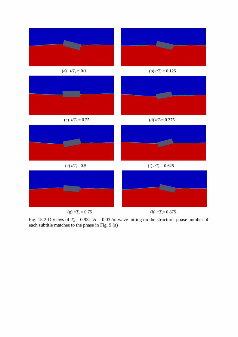
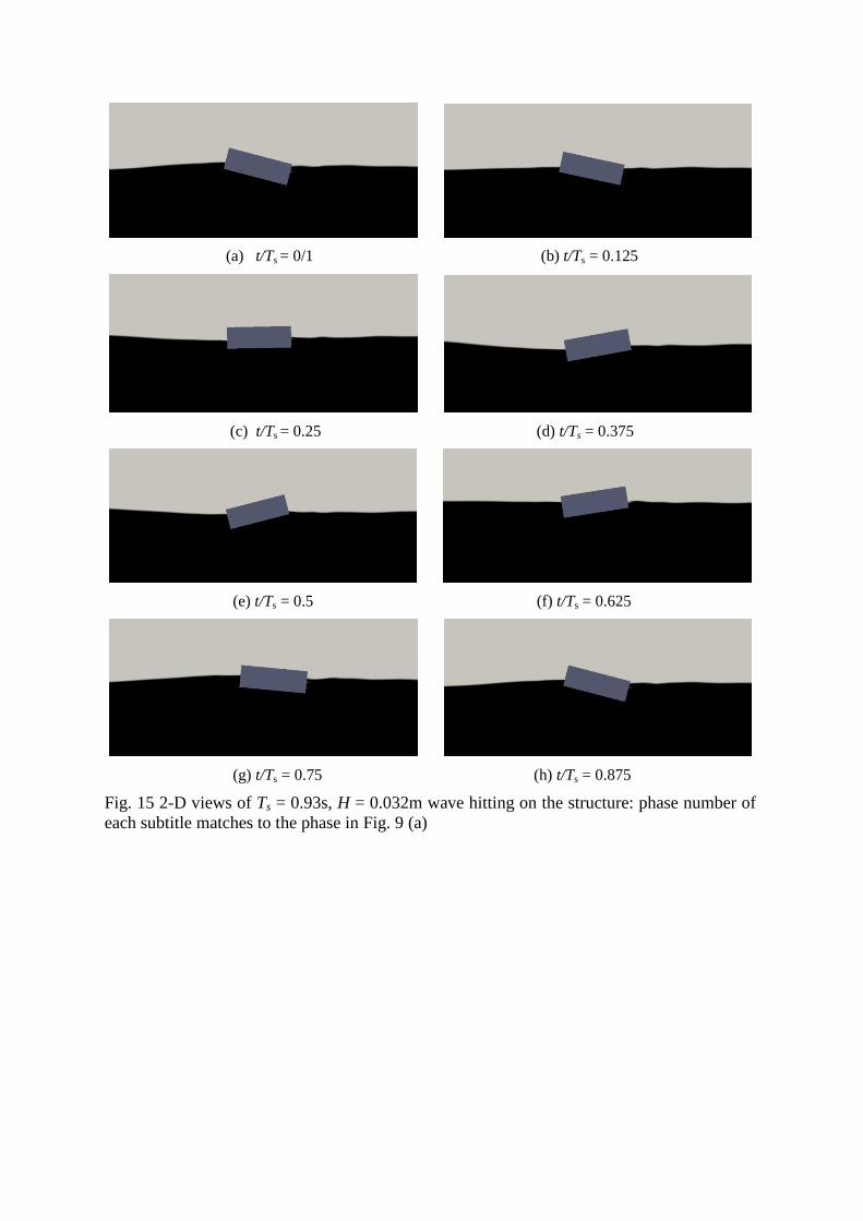
period. In order to give more vivid impressions, Fig. 15 shows several snapshots of the 2-D
wave field around the structure for the case with Ts = 0.93 s, H = 0.032 m according to phases,
as shown in Fig. 8 (a).
3.3.2 Forces impacting on the structure
The horizontal (Fx) and vertical forces (Fz) impacting on the rectangular structure are shown
in Fig. 16 and Fig. 17, respectively, together with the wave elevations of ηs and ηL on the
seaward and leeward sides at different wave periods in one periods. It can be seen that
regardless of the wave periods, the positive values of Δη = ηs - ηL lead to positive forces and
vice versa, which means that the sign and magnitude of forces are determined by the
difference in wave elevations at the left and right hand side of the structure. Especially, in the
cases of Ts = 0.93 s and Ts = 0.7 s, the time behaviour of forces are mainly determined by the
change of ηs on the seaward side due to the little variation in ηL as shown in Figs. 16 (a) – (b)
and Figs . 17 (a) – (b) for Ts = 0.93 s and Ts = 0.7 s, respectively.
The relation between forces and the difference in wave elevations on the seaward and
leeward sides with respect to the wave height has been studied and shown in Figs. 18 - 19,
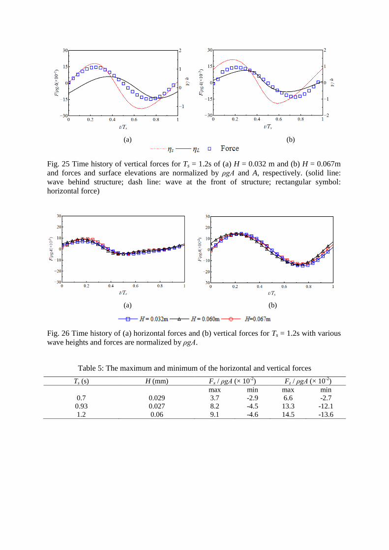
Figs. 21 – 22 and Figs. 24 – 25 for Ts = 0.93 s, Ts = 0.7 s and Ts = 1.2 s, respectively. Not
surprisingly, the time behaviour of forces impacting on the structure is independent of the
wave heights of the incoming waves for all three wave periods while is determined by the
difference in wave heights of the wave on the seaward and leeward sides of the structure. It is
interesting to find that the normalized forces in both horizontal and vertical direction have
similar values at different wave heights even for cases with Ts = 0.93 s, which is very close to
the roll natural period of the rectangular structure, as shown in Fig. 20, Fig. 23 and Fig. 26 for
Ts = 0.93 s, Ts = 0.7 s and Ts = 1.2 s, respectively. This means that the nonlinear effect for
wave loading is less significant when compared with wave-induced roll motion. Additionally,
as with wave elevation and roll motion, phase difference in wave loading at different wave
heights is observed and for all three wave periods, the phase difference in cases of Ts = 1.2 s
is smallest, consistent with what has been observed in Figs. 12 – 14.

15
The maximum and minimum values of both horizontal and vertical forces for all three wave
periods, Ts = 0.93 s H = 0.027 m, Ts = 0.7 s H = 0.029 m and Ts = 1.2 s H =0.06 m, are
summarized in Table 5. The forces are normalized by ρgA, A is the wave amplitude.
Generally, the magnitude of forces increases with the increase of wave periods, while the
variations between the cases with the natural period of Ts = 0.93 s and the longer wave period
of Ts = 1.2 s is not significant.
A study has been conducted in order to determine the relation of wave loading hitting fixed
and floating structures with the same cross section in the same sea conditions, as shown in
Fig. 27. This suggests that for all the cases considered the wave loading on fixed structures
has close matching in both crest values and the shapes with those of floating structures.
3.3.3 Velocity and vorticity fields
An interesting finding in Fig. 7 is that the RAOs obtained from the linear potential theory
agree well with those obtained from the experiments and viscous-flow solver for shorter
waves (ω > ωN), but the linear potential theory clearly underestimates the RAOs for longer
waves (ω < ωN). Further investigations have been carried out for long wave with period of Ts
= 1.2 s to explain this phenomena. The velocity and vorticity fields of Ts = 1.2 s (ω/ωN =
0.775), H = 0.032 m wave close to both sides of the 2-D barge are shown in Fig. 28. Subplots
in Fig. 28 are named from (a) to (l), which matches the phases of the roll motion shown in
Fig. 8 (c). The barge reaches its maximum clockwise motion at Fig. 28 (a) and experienced
counter-clockwise motion from Figs. 28 (b) – (g). It can be seen from Fig. 28 (a) that the
negative vortex (black) exists at the seaward side of the structure and after a short period of
time, the negative vortex (black) diffuses and a positive vortex (white) appears and is staying
during the rollaway motion from Figs. 28 (b) – (g). At the right hand side of the structure, the
positive vortex (white) decays and the negative vortex (black) increases during the rollaway
cycle. The barge reaches its maximum counter-clockwise position at Fig. 28 (h) and
experiences clockwise motion from Figs. 28 (i) – (l). Similar to the counter-clockwise motion,
the positive vortex diffuses quickly and a negative vortex develops at the left hand side of the
structure. In contrast to the seaward side, the negative vortex decays while the positive vortex
appears and is remaining during the roll-in cycle near the left bottom corner on the leeward
side. A similar mechanism was observed by Jung et al. [8] and they explained that since the
position of the positive vortex is “ahead” of the rolling direction of the structure during most

16
of the cycle, the structure experiences “negative” damping, i.e., the viscous effect increases
the roll motion at lower frequencies rather than damping it out which is observed in Fig. 7.
3.3.4 Parametric studies
Numerical studies have been carried out to investigate the dependence of roll motion on body
draft, height and breadth. The cross section used in previous section or experiments described
by Jung et al. [8] is chosen as standard case, and the depth and breadth of the object are
labelled as D and B, respectively. A new parameter ε, the ratio in characteristic length of new
cross sections and the standard case, is introduced to describe the change in cross section and
draft. That is, ε = d/D, a/D and b/B for cases with various drafts, body heights and body
widths, respectively. Here, d, a and b represent the depth of the body under the water surface,
one half of depth and width of new cross sections, respectively.
Influence of body draft
In order to investigate the influence of body draft on the roll motion, three different drafts ε
= d/D = 0.375, 0.5 and 0.625 are considered with the same body breadth B = 0.3 m and body
height D = 0.1 m. ε = 0.5 means that the structure is half submerged. Variations of the
magnification factors of the rectangular barge with the incident wave frequencies ω for all
three drafts are shown in Fig. 29. It can be seen that the roll motions for a 2-D rectangular
barge increase gradually with ω at lower frequencies and reach its maximum between ω =
6.4 rad/s and ω = 7.4 rad/s for different ε. The roll motions then decrease with the increase of
the ω afterwards. Additionally, the natural frequency ωN, corresponding response frequency
of the maximal roll motion, tends to decrease with the increase of body draft and the peak
value of the roll motion for the cases ε = 0.5 is the largest among three drafts and the smallest
roll motion occurs when ε = 0.375. Generally, the roll motions at lower frequencies are larger
than those at higher frequencies. For waves with lower frequencies, the roll motions for ε =
0.625 are larger than those of ε = 0. 375 cases and cases with ε = 0.5 sit in between. However,
for waves with higher frequencies, the trend is opposite, i.e. the roll motions for ε = 0.625 are
smaller than those of ε = 0.375 cases. It means that for longer wave conditions, the deep-draft
barge is less stable than the shallow-draft barge, and vise versa for shorter wave, which is
consistent with the conclusions presented by Chen et al. [47]. They argued that in order to
minimize the wave-induced roll motion, engineers from oil and gas industry or ship
companies need to adjust the deck loading so that the natural frequency can be moved away
from the dominant frequency of the ambient sea conditions.

17
Influence of body height
The variation of roll motion with the incident wave frequencies ω, concerning the influence
of body height is investigated in this section. Three body heights are considered, i.e. ε = a/D
= 0.375, 0.5 and 0.625 with the same draft d = 0.05 m and body breadth B = 0.3 m.
Variations of the magnification factors of the rectangular barge with the incident wave
frequencies ω for all three body heights are shown in Fig. 30. Similar trends to cases
concerning the influence of body draft are observed. It can be seen from Fig. 30 that the
motions increase gradually with the increase of ω and reach their maximum at the natural
frequencies, which decrease with the increase of body height. Again, the maximum and
minimum peak values of the roll motion are observed when ε = 0.5 and ε = 0.375 among
cases with all three body heights, respectively. The roll motions at lower frequencies are
generally larger than those at higher frequencies. And at lower frequencies, the larger the
body height is the larger the roll motion, and vise versa for waves with higher frequencies.
Influence of body breadth
The influence of body breadth on the natural frequency and the roll motion of a 2-D barge is
studied here with three different body breadths, i.e. ε = 0.375, 0.5 and 0.625 with the same
draft d = 0.05 m and body height D = 0.1 m. Variations of the RAOs of the rectangular barge
with the incident wave frequencies ω for all three body breadth are shown in Fig. 31. It can
be seen from the graph that the roll motions increase gradually with the increase of ω until
reach its maximum values at the natural frequencies and the roll motions at lower frequencies
are larger than those at higher frequencies, which are also observed in Fig. 29 and 30. The
natural frequency for cases with smaller breadth is lower than those with larger breadth while
the trend for the corresponding roll motion is opposite, i.e. the peak value of the roll motion
for ε = 0.375 is the largest. Additionally, the roll motions for the cases with smaller body
breadth is larger than those with larger body breadth for longer wave conditions, and vise
versa for shorter waves.
4. Conclusions
OpenFOAM has been further extended and used in the present study to model the roll motion
of a 2-D rectangular barge under wave actions. The modules developed in [28; 29] have been
selected here for wave generation and absorbing. The wave generation is via the flux into the
computational domain through a vertical wall. The velocities from the 2nd
order Stokes’ wave
theory are used for generating regular waves and the numerical beach is applied to minimize

18
wave reflection at the end of the wave tank. The viscous-flow solver for multiphase problems
with moving mesh, interDyMFoam, supplied with OpenFOAM, has been extended for
predicting roll motions of floating structures. The new locations of the floating structures are
determined by solving the equations of motion using the ODE solver supplied with
OpenFOAM based on fifth-order Cash-Karp Runge-Kutta method.
Comparisons among the present numerical results, potential-flow results given in the paper [8]
and the measured data collected by Jung et al. [8] have indicated that the extended
OpenFOAM used in the present study is very capable of accurate modelling of wave
interaction with freely rolling structures, with the natural frequency and roll motion correctly
captured. However, the potential flow theory over-predicts the roll motion significantly at the
natural frequency and underestimates the roll motion at lower frequencies due to the fact that
the viscous damping is not taken into account in the potential flow theory.
The roll motion increases gradually with the increase of the incident wave frequency until
reach its maximum values at the natural frequency. It is also found that at the natural
frequency, the magnification factors for roll motion decrease with the increase of the incident
wave height while for wave frequencies away from the natural frequency, the magnification
factors have the similar values, i.e. the nonlinear effect on the roll damping is significant only
for the natural frequency. With respect to the wave loading on the structures, the time
behavior of normalized forces are determined by the difference in wave free surface
elevations on the seaward and leeward sides of the structure regardless of wave periods and
wave heights of incoming waves. Additionally, the investigation on the velocity and vorticity
fields reveals that the viscous effect not only can damp out the roll motion but also can help
the structure to roll.
The parametric study has been carried out to shed some insight on the influence of body draft,
height and breadth on the roll motion of a 2-D rectangular barge. These new results have
revealed that the natural frequency increases with the increase of body breadth while
decreases with the increase of body draft and height. The largest peak values of the roll
motion at the natural frequency are observed for the cases with the smallest body breadth or
for the cases with medium body draft and height. Moreover, at lower frequencies, the roll
motion is general larger than that at higher frequencies.
Acknowledgments

19
Authors are very grateful for the reviewers’ constructive comments and suggestions, which
have helped to improve the quality of this paper. The first author acknowledges the financial
support of the University of Bath and China Scholarship Council (CSC) for her PhD study.
Authors are also grateful for the use of the HPC facility at University of Bath for some of the
numerical analysis.
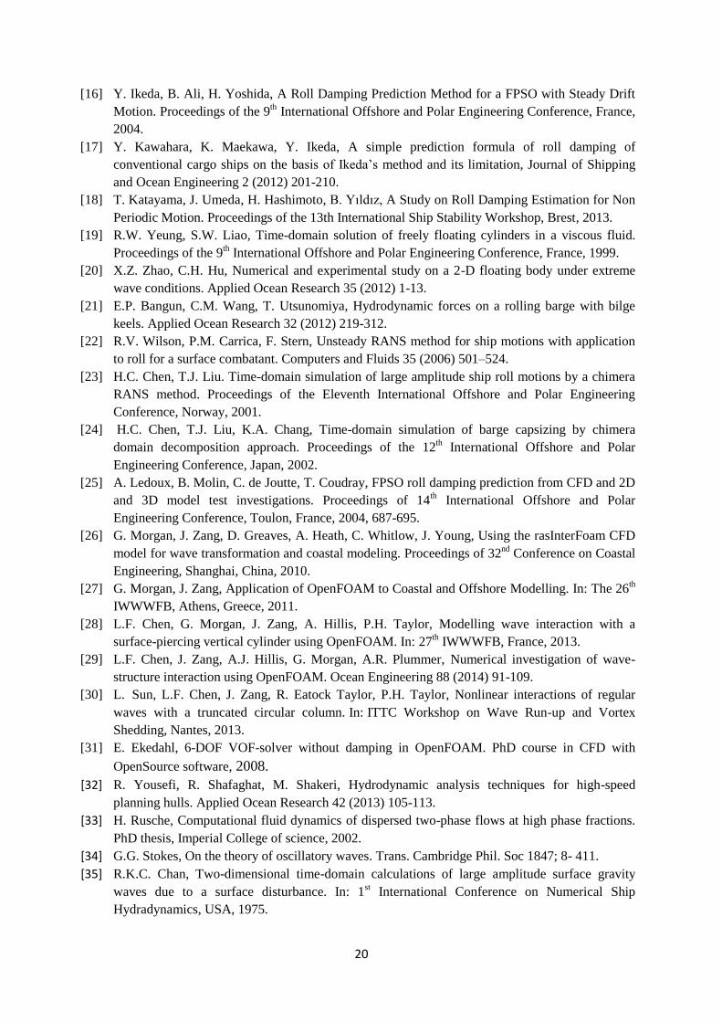
References
[1] S. Surendran, J. Venkata Ramana Reddy, Numerical simulation of ship stability for dynamic
environment. Ocean Engineering 30 (2003) 1305-1317.
[2] M. Taylan, The effect of nonlinear damping and restoring in ship rolling. Ocean Engineering 27
(2000) 21-932.
[3] R. Bhattacharyya, Dynamics of marine vehicles. Wiley; New York, 1978.
[4] J.H. Vugts, Pitch and heave with fixed and controlled bow fins. International Shipbuilding
Progress 15 (1967) 191-215.
[5] Y. Himeno, Prediction of ship roll damping - state of the art. Report No. 239, Department of
Naval Architecture and Marine Engineering, The University of Michigan, Ann Arbor, MI.
September, 1981.
[6] Y.R. Choi, J.H. Kim, M.J. Song, Y.S. Kim, An experimental and numerical study of roll motions
for a barge type LNG FPSO. Proceedings of the 14th International Offshore and Polar
Engineering Conference, Toulon, France, 2004; 672-675.
[7] K.H. Jung, K.A. Chang, H.C. Chen, E.T. Huang. Flow analysis of rolling rectangular barge in
beam sea condition. Proceeding of the 13th International Offshore and Polar Engineering
Conference, Honolulu, Hawaii, 2003.
[8] K.H. Jung, K.A. Chang, H.J. Jo, Viscous effect on the roll motion of a rectangular structure.
Journal of Engineering Mechanics 132 (2006) 190-200.
[9] X. Wu, L. Tao, Y. Li, Nonlinear roll damping of ship motions in waves. Journal of Offshore
Mechanics and Arctic Engineering 127 (2005) 205-211.
[10] J.M.J Journée, Quick strip theory calculations in ship design. In: conference on Practical Design
of Ships and Mobile Structures, Newcastle upon Tyne, U.K., 1992.
[11] R.T. Schmitke, Ship sway, roll and yaw motions in oblique seas. SNAME Transactions 86 (1978)
26-46.
[12] J.H. Lee, A. Incecik, The simplified method for the prediction of radiation damping coefficients.
Proceedings of the 16th International Offshore and Polar Engineering Conference, Lisbon,
Portugal, 2007; 2178-2183.
[13] S. Chakrabarti, Empirical calculation of roll damping for ships and barges. Ocean Engineering 28
(2001) 915-932.
[14] M. Downie, J. Graham, X. Zheng. Effect of viscous damping on the response of floating bodies.
Proceedings of the 18th Symposium on Naval Hydrodynamics, Ann Arbor, Michigan, 1991; 149-
155.
[15] Y. Ikeda, Y. Himeno, N. Tanaka, A prediction method for ship rolling. Department of Naval
Architecture, University of Osaka Prefecture, Japan, Report 00405, 1978.
20
[16] Y. Ikeda, B. Ali, H. Yoshida, A Roll Damping Prediction Method for a FPSO with Steady Drift
Motion. Proceedings of the 9th International Offshore and Polar Engineering Conference, France,
2004.
[17] Y. Kawahara, K. Maekawa, Y. Ikeda, A simple prediction formula of roll damping of
conventional cargo ships on the basis of Ikeda’s method and its limitation, Journal of Shipping
and Ocean Engineering 2 (2012) 201-210.
[18] T. Katayama, J. Umeda, H. Hashimoto, B. Yıldız, A Study on Roll Damping Estimation for Non
Periodic Motion. Proceedings of the 13th International Ship Stability Workshop, Brest, 2013.
[19] R.W. Yeung, S.W. Liao, Time-domain solution of freely floating cylinders in a viscous fluid.
Proceedings of the 9th International Offshore and Polar Engineering Conference, France, 1999.
[20] X.Z. Zhao, C.H. Hu, Numerical and experimental study on a 2-D floating body under extreme
wave conditions. Applied Ocean Research 35 (2012) 1-13.
[21] E.P. Bangun, C.M. Wang, T. Utsunomiya, Hydrodynamic forces on a rolling barge with bilge
keels. Applied Ocean Research 32 (2012) 219-312.
[22] R.V. Wilson, P.M. Carrica, F. Stern, Unsteady RANS method for ship motions with application
to roll for a surface combatant. Computers and Fluids 35 (2006) 501–524.
[23] H.C. Chen, T.J. Liu. Time-domain simulation of large amplitude ship roll motions by a chimera
RANS method. Proceedings of the Eleventh International Offshore and Polar Engineering
Conference, Norway, 2001.
[24] H.C. Chen, T.J. Liu, K.A. Chang, Time-domain simulation of barge capsizing by chimera
domain decomposition approach. Proceedings of the 12th International Offshore and Polar
Engineering Conference, Japan, 2002.
[25] A. Ledoux, B. Molin, C. de Joutte, T. Coudray, FPSO roll damping prediction from CFD and 2D
and 3D model test investigations. Proceedings of 14th International Offshore and Polar
Engineering Conference, Toulon, France, 2004, 687-695.
[26] G. Morgan, J. Zang, D. Greaves, A. Heath, C. Whitlow, J. Young, Using the rasInterFoam CFD
model for wave transformation and coastal modeling. Proceedings of 32nd
Conference on Coastal
Engineering, Shanghai, China, 2010.
[27] G. Morgan, J. Zang, Application of OpenFOAM to Coastal and Offshore Modelling. In: The 26th
IWWWFB, Athens, Greece, 2011.
[28] L.F. Chen, G. Morgan, J. Zang, A. Hillis, P.H. Taylor, Modelling wave interaction with a
surface-piercing vertical cylinder using OpenFOAM. In: 27th IWWWFB, France, 2013.
[29] L.F. Chen, J. Zang, A.J. Hillis, G. Morgan, A.R. Plummer, Numerical investigation of wave-
structure interaction using OpenFOAM. Ocean Engineering 88 (2014) 91-109.
[30] L. Sun, L.F. Chen, J. Zang, R. Eatock Taylor, P.H. Taylor, Nonlinear interactions of regular
waves with a truncated circular column. In: ITTC Workshop on Wave Run-up and Vortex
Shedding, Nantes, 2013.
[31] E. Ekedahl, 6-DOF VOF-solver without damping in OpenFOAM. PhD course in CFD with
OpenSource software, 2008.
[32] R. Yousefi, R. Shafaghat, M. Shakeri, Hydrodynamic analysis techniques for high-speed
planning hulls. Applied Ocean Research 42 (2013) 105-113.
[33] H. Rusche, Computational fluid dynamics of dispersed two-phase flows at high phase fractions.
PhD thesis, Imperial College of science, 2002.
[34] G.G. Stokes, On the theory of oscillatory waves. Trans. Cambridge Phil. Soc 1847; 8- 411.
[35] R.K.C. Chan, Two-dimensional time-domain calculations of large amplitude surface gravity
waves due to a surface disturbance. In: 1st International Conference on Numerical Ship
Hydradynamics, USA, 1975.

21
[36] J.E. Romate, Absorbing boundary conditions for free surface waves. Journal of computational
physics 99 (1992) 135-145.
[37] R. de Bruijun, F. Huijs, R. Huijsmans, T. Bunnik, M. Gerritsma, Calculation of wave forces and
internal loads on a semi-submersible at shallow draft using an IVOF method. Proceedings of the
ASME 2011 30th International Conference on Ocean, Offshore and Arctic
Engineering,Rotterdam, The Netherlands, 2011.
[38] P. Kaps, P. Rentrop, Generalized Runge-Kutta Methods of order four with stepsize control for
stiff ordinary differential equations. Numerische Mathematik 33 (1979) 55-68.
[39] G. Bader, P. Deuflhard, A semi-implicit mid-point rule for stiff systems of ordinary differential
equations. Numerische Mathematik 41 (1983) 373-398.
[40] W.H. Press, S.A. Teukolsky, W.T. Vettering, B.P. Flannery, Numerical Recipes: The art of
scientific computing. Press Syndicate of the University of Cambridge, 1992.
[41] J.R. Cash, A.H. Karp, A variable order Runge-Kutta method for initial value problems with
rapidly varying right-hand sides. ACM transactions on mathematical software 1990; 16: 201-222.
[42] Jasak H, Tukovic Z. Automatic mesh motion for the unstructured finite volume method.
Transactions of FAMENA 30 (2007) 1-18.
[43] The OpenFOAM® Foundation. The open source CFD toolbox of OpenFOAM: User Guide. 2011.
[44] R. Courant, K. Friedrichs, H. Lewy, On the partial difference equations of mathematical physics.
IBM Journal of Research and Development 11 (1967) 215-234.
[45] J. Ferziger, M. Peric, Computational Methods for Fluid Dynamics. 2nd
. Berlin: Springer; 1999.
[46] R.I. Issa, Solution of the implicitly discretised fluid flow equations by operator-splitting. Journal
of Computer Physics 62 (1985) 40-65.
[47] H.C. Chen, T.J. Liu, E.T. Huang, Time-domain simulation of large amplitude ship roll motions
by a chimera RANS method. Proceedings of the 11th International Offshore and Polar
Engineering Conference, Norway, 2001.
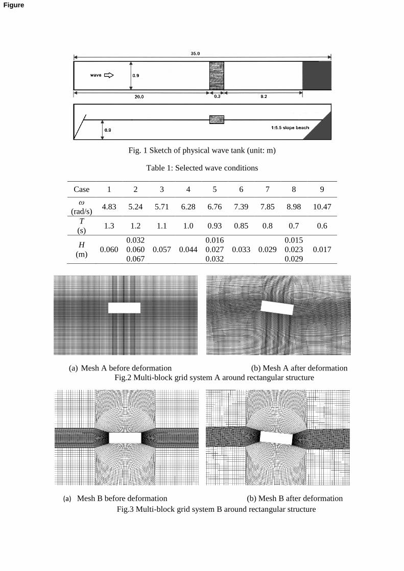
Fig. 1 Sketch of physical wave tank (unit: m)
Table 1: Selected wave conditions
Case 1 2 3 4 5 6 7 8 9
ω
(rad/s) 4.83 5.24 5.71 6.28 6.76 7.39 7.85 8.98 10.47
T
(s) 1.3 1.2 1.1 1.0 0.93 0.85 0.8 0.7 0.6
H
(m) 0.060
0.032
0.060
0.067
0.057 0.044
0.016
0.027
0.032
0.033 0.029
0.015
0.023
0.029
0.017
(a) Mesh A before deformation (b) Mesh A after deformation
Fig.2 Multi-block grid system A around rectangular structure
(a) Mesh B before deformation (b) Mesh B after deformation
Fig.3 Multi-block grid system B around rectangular structure
Figure

Table 2: Mesh parameters and corresponding results
Mesh
type Wave
Coarse area
(unit: m)
Refined area
(unit: m)
Roll motion
(φ/kA)
T = 0.93 s
L = 1.35 m
H = 0.016 m
d =0.9 m
Δx Δz Δx Δz Num Exp Error
Mesh A 0.02 0.005 0.005 0.0025 1.28
1.66
22.9%
Mesh B1 0.02 0.02 0.01 0.005 1.583 4.6%
Mesh B2 0.015 0.02 0.0075 0.005 1.583 4.6%
Mesh B3 0.02 0.02 0.01 0.01 1.383 16.7%
Fig. 4 Mesh convergent test
(a) Time history of angle of inclination (b) corresponding spectrum
Fig. 5 Test of roll free decay
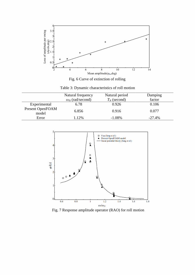
Fig. 6 Curve of extinction of rolling
Table 3: Dynamic characteristics of roll motion
Natural frequency
ωN (rad/second)
Natural period
TN (second)
Damping
factor
Experimental 6.78 0.926 0.106
Present OpenFOAM
model 6.856 0.916 0.077
Error 1.12% -1.08% -27.4%
Fig. 7 Response amplitude operator (RAO) for roll motion

(a) (b)
(c)
Fig. 8 Time histories of wave elevation (η) of incoming waves and rotating angle of the
rectangular structure (φ) at different wave periods and wave heights of (a) Ts = 0.93 s; H =
0.027 m, (b) Ts = 0.8 s; H = 0.029 m and (c) Ts = 1.2 s; H = 0.06 m. Rotating angle and
surface elevations are normalized by kA and A, respectively
(a) (b)
Fig. 9 Time histories of wave elevation (η) of incoming waves and rotating angle of the
rectangular structure (φ) at Ts = 0.93 s with different wave heights of (a) H = 0.016 m and (b)
H = 0.032 m. Rotating angle and surface elevations are normalized by kA and A, respectively
1 2 3 4 5 6 7 8 9 10 11 12 1
η φ η φ
η
φ
1 2 3 4 5 6 7 8 1

(a) (b)
(c)
Fig. 10 Time histories of wave elevation (η) of incoming waves and rotating angle of the
rectangular structure (φ) at Ts = 0.7 s with different wave heights of (a) H = 0.015 m, (b) H =
0.023 m and (c) H = 0.029 m. Rotating angle and surface elevations are normalized by kA
and A, respectively
(a) (b)
Fig. 11 Time histories of wave elevation (η) of incoming waves and rotating angle of the
rectangular structure (φ) at Ts = 1.2 s with different wave heights of (a) H = 0.032 m and (b)
H = 0.067 m. Rotating angle and surface elevations are normalized by kA and A, respectively

Table 4: Free surface elevation of incoming waves and rotating angle of the rectangular
structure at three different periods with three different wave heights
Ts
unit: s
ω
unit: rad/s ω/ ωN
A
unit: m
φ
unit: rad φ/A
0.93 6.76 1
0.008 0.159 19.875
0.0135 0.191 14.148
0.016 0.207 12.938
0.7 8.98 1.328
0.0075 0.0174 2.320
0.0115 0.0220 1.913
0.0145 0.0247 1.703
1.2 5.24 0.775
0.016 0.087 6.060
0.030 0.158 5.267
0.0335 0.176 5.254
Fig. 12 Wave profiles at the moment of t = 40Ts for Ts = 0.93s with different wave heights of
(a) H = 0.032 m, (b) H = 0.027 m and (c) H = 0.016 m and the dash lines represents the
location of the floating object.
Fig. 13 Wave profiles at the moment of t = 60Ts for Ts = 0.7s with different wave heights of
(a) H = 0.029 m, (b) H = 0.023 m and (c) H = 0.015 m and the dash lines represents the
location of the floating object.
(a)
(b)
(c)
(a)
(b)
(c)

Fig. 14 Wave profiles at the moment of t = 30Ts for Ts = 1.2s with different wave heights of
(a) H = 0.067 m, (b) H = 0.060 m and (c) H = 0.032 m and the dash lines represents the
location of the floating object.
(a)
(b)
(c)
(a) t/Ts = 0/1 (b) t/Ts = 0.125
(c) t/Ts = 0.25 (d) t/Ts= 0.375
(e) t/Ts= 0.5 (f) t/Ts = 0.625
(g) t/Ts = 0.75 (h) t/Ts= 0.875
Fig. 15 2-D views of Ts = 0.93s, H = 0.032m wave hitting on the structure: phase number of
each subtitle matches to the phase in Fig. 9 (a)
(a) t/Ts = 0/1 (b) t/Ts = 0.125
(c) t/Ts = 0.25 (d) t/Ts = 0.375
(e) t/Ts = 0.5 (f) t/Ts = 0.625
(g) t/Ts = 0.75 (h) t/Ts = 0.875
Fig. 15 2-D views of Ts = 0.93s, H = 0.032m wave hitting on the structure: phase number of
each subtitle matches to the phase in Fig. 9 (a)

(a) (b)
(c)
Fig. 16 Time history of horizontal forces for (a) Ts = 0.93s and H = 0.016 m, (b) Ts = 0.7s
and H = 0.029 m and (c) Ts = 1.2s and H = 0.060 m and forces and surface elevations are
normalized by ρgA and A, respectively. (solid line: wave behind structure; dash line: wave at
the front of structure; rectangular symbol: horizontal force)

(a) (b)
(c)
Fig. 17 Time history of vertical forces for (a) Ts = 0.93s and H = 0.016 m, (b) Ts = 0.7s and H
= 0.029 m and (c) Ts = 1.2s and H = 0.060 m and forces and surface elevations are
normalized by ρgA and A, respectively. (solid line: wave behind structure; dash line: wave at
the front of structure; rectangular symbol: vertical force)
(a) (b)
Fig. 18 Time history of horizontal forces for Ts = 0.93s of (a) H = 0.027 m and (b) H = 0.032
m and forces and surface elevations are normalized by ρgA and A, respectively. (solid line:
wave behind structure; dash line: wave at the front of structure; rectangular symbol:
horizontal force)

(a) (b)
Fig. 19 Time history of vertical forces for Ts = 0.93 s of (a) H = 0.027 m and (b) H = 0.032m
and forces and surface elevations are normalized by ρgA and A, respectively. (solid line:
wave behind structure; dash line: wave at the front of structure; rectangular symbol:
horizontal force)
(a) (b)
Fig. 20 Time history of (a) horizontal forces and (b) vertical forces for Ts = 0.93s with
various wave heights and forces are normalized by ρgA.
(a) (b)
Fig. 21 Time history of horizontal forces for Ts = 0.7s of (a) H = 0.015 m and (b) H = 0.023m
and forces and surface elevations are normalized by ρgA and A, respectively. (solid line:
wave behind structure; dash line: wave at the front of structure; rectangular symbol:
horizontal force)

(a) (b)
Fig. 22 Time history of vertical forces for Ts = 0.7s of (a) H = 0.015 m and (b) H = 0.023m
and forces and surface elevations are normalized by ρgA and A, respectively. (solid line:
wave behind structure; dash line: wave at the front of structure; rectangular symbol:
horizontal force)
(a) (b)
Fig. 23 Time history of (a) horizontal forces and (b) vertical forces for Ts = 0.7s with various
wave heights and forces are normalized by ρgA.
(a) (b)
Fig. 24 Time history of horizontal forces for Ts = 1.2s of (a) H = 0.032 m and (b) H = 0.067m
and forces and surface elevations are normalized by ρgA and A, respectively. (solid line:
wave behind structure; dash line: wave at the front of structure; rectangular symbol:
horizontal force)
(a) (b)
Fig. 25 Time history of vertical forces for Ts = 1.2s of (a) H = 0.032 m and (b) H = 0.067m
and forces and surface elevations are normalized by ρgA and A, respectively. (solid line:
wave behind structure; dash line: wave at the front of structure; rectangular symbol:
horizontal force)
(a) (b)
Fig. 26 Time history of (a) horizontal forces and (b) vertical forces for Ts = 1.2s with various
wave heights and forces are normalized by ρgA.
Table 5: The maximum and minimum of the horizontal and vertical forces
Ts (s) H (mm) Fx / ρgA (× 10-2
) Fz / ρgA (× 10-2
)
max min max min
0.7 0.029 3.7 -2.9 6.6 -2.7
0.93 0.027 8.2 -4.5 13.3 -12.1
1.2 0.06 9.1 -4.6 14.5 -13.6

(a)
(b)
(c)
Fig. 27 Time history of forces on fixed rectangular (solid line) and rotating rectangular (Ο) for
(a) Ts = 0.93s and H = 0.016 m, (b) Ts = 0.7s and H = 0.015 m and (c) Ts = 1.2s and H =
0.032 m
Fz
Fx
Fz
Fx
Fz
Fx

(a) t/Ts = 0/0.996 (b) t/Ts= 0.083
(c) t/Ts = 0.166 (d) t/Ts = 0.249
(e) t/Ts = 0.332 (f) t/Ts = 0.415
(g) t/Ts = 0.498 (h) t/Ts = 0.581
(i) t/Ts = 0.664 (j) t/Ts = 0.747
(k) t/Ts = 0.83 (j) t/Ts = 0.913
Fig. 28 Vorticity and velocity field of Ts = 1.2s, H = 0.032m wave: phase number of each
subtitle matches to the phase in Fig. 9 (c)

Figure 29: Magnification factors for roll motion for cases with all three drafts (ε = d/D, d is
draft and D is depth of the object)
Figure 30: Magnification factors for roll motion for cases with all three body heights (ε = a/D,
a is half of depth of the object)
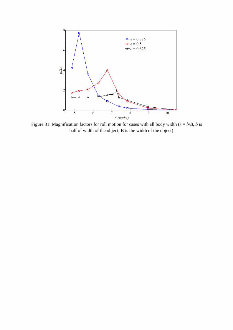
Figure 31: Magnification factors for roll motion for cases with all body width (ε = b/B, b is
half of width of the object, B is the width of the object)