Ann. Henri Poincare 17 (2016), 2623–2662c© 2016 The Author(s). This article is publishedwith open access at Springerlink.com1424-0637/16/102623-40published online March 30, 2016

DOI 10.1007/s00023-016-0469-6 Annales Henri Poincare

Elliptic Genera and 3d Gravity

Nathan Benjamin, Miranda C. N. Cheng, Shamit Kachru,Gregory W. Moore and Natalie M. Paquette

Abstract. We describe general constraints on the elliptic genus of a 2d su-persymmetric conformal field theory which has a gravity dual with largeradius in Planck units. We give examples of theories which do and do notsatisfy the bounds we derive, by describing the elliptic genera of symmet-ric product orbifolds of K3, product manifolds, certain simple familiesof Calabi–Yau hypersurfaces, and symmetric products of the “MonsterCFT”. We discuss the distinction between theories with supergravity du-als and those whose duals have strings at the scale set by the AdS cur-vature. Under natural assumptions, we attempt to quantify the fractionof (2,2) supersymmetric conformal theories which admit a weakly curvedgravity description, at large central charge.

1. Introduction

The AdS/CFT correspondence [1] provides a concrete framework for hologra-phy, where very particular d dimensional quantum field theories can capturethe dynamics of quantum gravity in d + 1 spacetime dimensions. A naturalquestion from the outset has been: “which class of quantum field theories isdual to (large radius, weakly coupled) Einstein gravity theories?”

In a recent paper [2], interesting progress was made on this issue in theparticular case of two-dimensional CFTs. The authors of [2] make the plausibleassumption that a weakly coupled gravitational theory should reproduce themost basic aspects of the phase structure known in all of the simple examplesof AdS/CFT. In particular, as one raises the temperature, there should be aphase transition at a critical temperature (usually taken to be β∗ = 1

kT ∗ = 2π)between a “gas of particles” and a black hole geometry [3]—the Hawking–Pagetransition [4]. By requiring that outside a small neighborhood of the criticaltemperature the thermal partition function should be dominated by BTZ black

M. C. N. Cheng: On leave from CNRS, France.

2624 N. Benjamin et al. Ann. Henri Poincare

holes at high T , or the ground state at low T , one finds interesting constraintson the spectrum of any putative dual conformal field theory.

A significant consequence of this constraint is the derivation of theBekenstein–Hawking black hole entropy (expressed here in the ensemble whereone keeps track only of the total energy E = h + h − c

12 )

S(E) ∼ 2π

√cE

3, E = h + h − c

12(1.1)

for E > c12 and c � 1. Notice that this is the regime where we expect the

Bekenstein–Hawking formula to give a good approximation of the black holeentropy on gravitational grounds. It is different from the regime of applicabilityof the usual Cardy formula based on familiar modular form arguments (E

c �1).

Here, we turn our attention to 2d supersymmetric theories. In two-dimensional theories with at least (0, 1) supersymmetry and left and right-moving Z2 fermion number symmetries, one can define the elliptic genus [5–8].We will focus on the special case of (2, 2) supersymmetry in this paper, but weexpect that many of our considerations could be suitably generalized. In the(2, 2) case, the elliptic genus associates to a 2d SCFT a weak Jacobi form; de-tailed knowledge of the space of such forms (see e.g., [9]) will allow us to makesome strong statements about CFT/gravity duality in this case. Prominentcases of such 2d supersymmetric theories in the AdS/CFT correspondence in-clude those arising in D-brane constructions of supersymmetric black strings[10], where the near-horizon geometry has a dual given by a σ-model withtarget MN/SN for M = K3 or T 4. By requiring the Bekenstein–Hawkingformula for these black objects to apply in the black hole regime, we derive aconstraint on the coefficients of the elliptic genus.

Intuitively, the condition that the CFT elliptic genus exhibits an enlargedregime of applicability of the Bekenstein–Hawking entropy (which turns outto warrant a Hawking–Page transition) hints that there is indeed a weaklycoupled gravity dual. In the simplest perturbative string theory constructionsof AdS, there are at least three scales of interest—the Planck scale MPlanck,the string scale Mstring, and the inverse AdS radius 1

�AdS. (There are also in

general one or more Kaluza–Klein scales—for simplicity we are imagining con-structions like the Freund–Rubin construction where the KK scale coincideswith the AdS radius.) The most conventional regime of understanding stringmodels is when MPlanck � Mstring � 1

�AdS. However, the conditions we impose

are also satisfied in some theories where there is no separation of scales be-tween Mstring and 1

�AdSapparent in the elliptic genus. We therefore also discuss

further criteria on the coefficients of the elliptic genus which may distinguishbetween theories with a separation of scales between supergravity and stringmodes, and theories without such separation.

It is important to keep in mind that our necessary condition serves onlyas an indicator of whether there might be a weakly coupled gravity dual tosome region in the moduli space of the superconformal field theory. In simpleexamples, the moduli space will have other generic phases characterized by

Vol. 17 (2016) Elliptic Genera and 3d Gravity 2625

duals with no simple geometric description, and the large radius gravity dualwould characterize only a small region of the SCFT moduli space. However, asthe elliptic genus is an invariant calculable (in principle) in this small region, itwill have the properties expected of a theory with a weakly coupled gravity de-scription if the SCFT admits such a description anywhere in its moduli space.

This paper is organized as follows. In Sect. 2, we review some basic factsabout Jacobi forms. In Sect. 3, we describe the constraint we wish to place onthe Fourier coefficients of these forms, following a similar philosophy to [2]. InSect. 4, we check the bound on various simple constructions: K3 symmetricproduct orbifolds (which provide some of the simplest examples of AdS3/CFT2

and do satisfy the bound), product manifolds, a family of Calabi–Yau spacesgoing off to large dimension, and a symmetric product of the “Monster CFT”.As some of the examples will fail, we see that the bound does have teeth—there are simple examples of (2,2) superconformal field theories at large cen-tral charge that violate it. In Sect. 5, focusing on the distinctions betweenthe K3 symmetric product and the “Monster” symmetric product, we discussthe distinction between low-energy supergravity theories and low-energy stringtheories. In Sect. 6, we attempt to quantify “the fraction of supersymmetrictheories at large central charge which admit a gravity dual”, using a naturalmetric on a relevant (suitably projectivized) space of weak Jacobi forms. De-tailed arguments supporting some of the assertions in the main body of thepaper are provided in two appendices.

2. Modularity Properties

We can define the following elliptic genera for any 2d SCFT with at least(1, 1) supersymmetry and left and right-moving fermion quantum numbers.Denote by Ln, Ln the left and right Virasoro generators, and F, F the left andright-moving fermion number. The NS sector elliptic genus can be defined via:

ZNS,+(τ) = TrNS,R (−1)FqL0−c/24qL0−c/24 . (2.1)

It is a (weakly holomorphic) modular form under the congruence subgroup Γθ,defined in (3.34). Similar definitions apply in other sectors:

χ = TrR,R (−1)F+FqL0−c/24qL0−c/24 (2.2)

ZR,+(τ) = TrR,R (−1)FqL0−c/24qL0−c/24 (2.3)

ZNS,−(τ) = TrNS,R (−1)F+FqL0−c/24qL0−c/24 . (2.4)

Here, q = e2πiτ where τ takes values in the upper-half plane, and we haveassumed equal left and right-moving central charges, cL = cR = c.

For the most part, we will consider theories with additional structure,e.g., (2, 2) superconformal theories. In fact for any (0, 2) theory with a left-moving U(1) symmetry, and so in particular for any (2, 2) SCFT, one candefine a refined elliptic genus as

ZR,R(τ, z) = TrR,R(−1)F+F qL0−c/24qL0−c/24yJ0 . (2.5)

2626 N. Benjamin et al. Ann. Henri Poincare

Here, y = e2πiz. The additional symmetry promotes the two-variable ellipticgenus into a weak Jacobi form [11]. We will also consider

ZNS,R(τ, z) = TrNS,R(−1)F qL0−c/24qL0−c/24yJ0

= ZR,R

(τ, z +

τ + 12

)q

c24 y

c6 . (2.6)

Note that we could define ZNS,NS as a quantity which localizes on right-movingchiral primaries, but with suitable definition it would give the same functionas ZNS,R above. So, while the AdS vacuum appears in the (NS,NS) sector, wewill focus on ZNS,R when stating our bounds in Sect. 3.

In the cases of interest to us, there is no anti-holomorphic dependence onτ due to the (−1)F insertion, and the elliptic genus is a purely holomorphicfunction of τ . In fact, much more is true. Using standard arguments one canshow that the elliptic genus of an SCFT defined above in (2.5) transforms nicelyunder the group Z

2�SL(2, Z). In particular, it is a so-called weak Jacobi form

of weight 0 and index c/6, defined below. For instance, supersymmetric sigmamodels for Calabi–Yau target spaces of complex dimension 2m have ellipticgenera that are weight 0 weak Jacobi form of index m. For the rest of thispaper, we will be considering SCFTs with m ∈ Z, or equivalently c divisibleby 6.

Consider a holomorphic function φ(τ, z) on H × C which satisfies theconditions

φ

(aτ + b

cτ + d,

z

cτ + d

)= (cτ + d)we2πim cz2

cτ+d φ(τ, z),(

a bc d

)∈ SL2(Z) (2.7)

φ(τ, z + �τ + �′) = e−2πim(�2τ+2�z)φ(τ, z), �, �′ ∈ Z . (2.8)

In the present context, (2.8) can be understood in terms of the spectral flowsymmetry in the presence of an N ≥ 2 superconformal symmetry.

The invariance φ(τ, z) = φ(τ + 1, z) = φ(τ, z + 1) implies a Fourier ex-pansion

φ(τ, z) =∑

n,�∈Z

c(n, �)qny�, (2.9)

and the transformation under ( −1 00 −1 ) ∈ SL2(Z) shows

c(n, �) = (−1)wc(n,−�). (2.10)

The function φ(τ, z) is called a weak Jacobi form of index m ∈ Z and weightw if its Fourier coefficients c(n, �) vanish for n < 0. Moreover, the elliptictransformation (2.8) can be used to show that the coefficients

c(n, �) = Cr(D(n, �)) (2.11)

depend only on the so-called discriminant

D(n, �) := �2 − 4mn (2.12)

and r = � (mod 2m). Note that D(n, �) is the negative of the polarity, definedin [12] as 4mn − �2.

Vol. 17 (2016) Elliptic Genera and 3d Gravity 2627

Combining the above, we see that a Jacobi form admits the expansion

φ(τ, z) =∑

r∈Z/2mZ

hm,r(τ)θm,r(τ, z) (2.13)

in terms of the index m theta functions,

θm,r(τ, z) =∑

k=r mod 2m

qk2/4myk. (2.14)

Both hm,r and θm,r only depend on the value of r modulo 2m. However, forsome later manipulations, we should note that it is sometimes useful to choosethe explicit fundamental domain −m < r ≤ m for the shift symmetry in r.When |r| ≤ m we can write:

hm,r(τ) = (−1)whm,−r(τ) =∑n≥0

c(n, r)q−D(n,r)/4m. (2.15)

The vector-valued functions θm,r(τ, z) transform as

θm

(−1

τ,− z

τ

)=

√−iτ e

2πimz2τ S θm(τ, z), (2.16)

θm(τ + 1, z) = T θm(τ, z), (2.17)

where S, T are the 2m × 2m unitary matrices with entries

Srr′ =1√2m

eπirr′

m , (2.18)

Trr′ = eπir22m δr,r′ . (2.19)

From this we see that h = (hm,r) is a 2m-component vector transforming as aweight w − 1/2 modular form for SL2(Z).

In particular, an elliptic genus (with w = 0) of a theory with centralcharge c = 6m can be written as

ZR,R(τ, z) =∑

r∈Z/2mZ

Zr(τ)θm,r(τ, z). (2.20)

We have written Zr(τ) for hm,r(τ) in this expression. Thus Zr(τ) only dependson r modulo 2m, but again, when |r| ≤ m it is useful to expand:

Zr(τ) = Z−r(τ) =∑n≥0

c(n, r)qn− r24m (2.21)

The function Zr(τ) can be thought of as the elliptic genus of the rth supers-election sector corresponding to the eigenvalue of J0 = r mod 2m. From theCFT point of view, the r ∼ r + 2m identification can be understood in termsof the spectral flow symmetry of the superconformal algebra. When there is agravity dual the r → r + 2m transformation corresponds, from the bulk view-point, to a large gauge transformation of a gauge field holographically dual tothe U(1)R.

Since the Fourier coefficients of a weak Jacobi form have to satisfy

c(n, �) = 0 for all n < 0, (2.22)

2628 N. Benjamin et al. Ann. Henri Poincare

(which can be thought of as unitarity of the CFT), this leaves open the possi-bility to have “polar terms” c(n, �)qny� with

m2 ≥ D(n, �) > 0, n ≥ 0

in an index m weak Jacobi form. These are called polar terms because theyare precisely the terms in the q-series of Zr(τ) that have exponential growthwhen approaching the cusp τ → i∞. The finite set of independent coefficientsof the polar terms in the elliptic genus will play a crucial role in what follows.In what follows, we will denote by φP the sum of all the polar terms in theelliptic genus.

Importantly, the full set of Fourier coefficients of a weak Jacobi form canbe reconstructed from just the polar part, φP . This can be understood throughthe fact that there are no non-vanishing negative weight modular forms at anylevel. For discussions of this in related contexts, see [12–14]. Let us denoteby Vm the space of possible polar polynomials (without requiring that theycorrespond to the polar part of a bona fide weak Jacobi form). Given thesymmetries of the c(n, �), Vm is spanned by qny� in the region P(m):

P(m) = {(�, n) : 1 ≤ � ≤ m, 0 ≤ n, D(n, �) > 0} . (2.23)

By a standard counting of the number of lattice points underneath the parabola4mn − �2 = 0 in the �, n plane [12], one can give a formula for the dimensionof the vector space of polar parts P (m) = dim(Vm):

P (m) =m∑

�=1

�2

4m�. (2.24)

In this note, where we work at leading order in large m, we will only needthe leading behavior of the sum (2.24); this is determined by the elementaryformula

∑m�=1 �2 = 1

3m3 + 12m2 + 1

6m to be

P (m) =112

m2 + O(m), m � 1. (2.25)

Because we are working at leading order at large m (large central charge),we will not need to use the subleading corrections to (2.25) (see for instance[9] and [12]). Neither will we need to deal with the important subtlety thatnot all vectors in Vm actually correspond to a weak Jacobi form. Denoting thespace of weak Jacobi forms of weight 0 and index m as J0,m, in fact one hasdim(J0,m) − P (m) = O(m). These facts would become important if one wereto extend our results to the next order in a 1/m expansion.

3. Gravity Constraints and Phase Structure

We will now derive a constraint on the polar coefficients of an SCFT as follows.The polar coefficients determine the elliptic genus, and we will require that thegenus matches the expected Bekenstein–Hawking entropy of black holes in thehigh-energy regime. Happily, we will find that a second (a priori independent)

Vol. 17 (2016) Elliptic Genera and 3d Gravity 2629

requirement of the existence of a sharp Hawking–Page transition at the criticaltemperature β = 2π gives the same constraint on the coefficients.

More precisely, we will be considering infinite sequences of CFTs goingoff to large central charge, and we will bound the asymptotic behavior ofphysical observables in such sequences as m → ∞. (One familiar example thatcan be taken as representative of what we have in mind is the sequence of σ-models with targets Symm(K3).) Simple physical considerations will lead usto propose certain constraints on the growth of the polar coefficients at largem in the related families of elliptic genera.

Now, there are precise mathematical statements on the behaviors of coef-ficients of large powers of q in modular forms. For instance, there are theoremsproving that for a generic holomorphic modular form f =

∑n cnqn of fixed

weight k, cn grows as O(nk−1) at large n, while for a cusp form, the coefficientsare of O(nk/2).

Note that our growth estimates are rather different in nature from those ofthe previous paragraph. Our estimates will be physically motivated by knownfacts about corrections to Einstein gravity in the expansion in energy dividedby MPlanck. We are proposing a mathematical criterion, motivated by physics,that would allow one to check whether a given sequence of CFTs can pos-sible have a weakly coupled gravity dual. This could equally well be viewedas a mathematical conjecture about the families of modular forms arising insequences with gravity duals.

Our eventual criterion will be derived by considering the free energiesFm of the CFTs in this family. The free energy in these theories, as m → ∞,gives a function with a sharp first-order phase transition at β = 2π. This isthe physical phenomenon of the Hawking–Page transition [4]. (Sharp roughlybecause, in microscopic examples of AdS3/CFT2, semi-classical configurationsof winding strings can condense and lower the free energy precisely at 2π,yielding the transition—see [§5.3.2, [15]]). Similarly, when we state physicallymotivated criteria about the free energies of our sequences of theories, wewill be making statements about the sequence Fm and assuming that thelimit as m → ∞ of 1

mFm exists as a piece-wise differentiable function withdiscontinuous first-derivative at β = 2π.

3.1. A Bekenstein–Hawking Bound on the Elliptic Genus

Suppose that φ is the elliptic genus of a superconformal field theory with alarge radius gravitational dual. Define the “reduced mass” of a particle statein the dual gravity picture to be the eigenvalue of

Lred0 = L0 − 1

4mJ2

0 − m

4, (3.1)

namely the quantity −D(n, �)/4m for the term qny� in the elliptic genus. DefineEred to be the eigenvalue under Lred

0 . Then:• Classically, the states with Ered > 0 are black holes in AdS3. We will

discuss their contribution to the supergravity computation of the ellipticgenus in detail below.

2630 N. Benjamin et al. Ann. Henri Poincare

• In contrast, in the gravitational computation of the elliptic genus, it isthe states with Ered < 0 which contribute to the polar part of the su-pergravity partition function [13]. These are precisely the modes whichare too light to form black holes in the bulk. These are the states whichappear in φP .

We now present an argument that constrains the coefficients in φP usingthe supergravity estimate of the black hole contribution to the elliptic genus.We treat the elliptic genus as the grand canonical partition function

Z(β, μ) =∑

microstates

eβ(μQ−E) = e−βF (β,μ), (3.2)

where τ = i β2π and z = −iβμ

2π are the corresponding variables in the ellipticgenus. In other words, we define

Z(β, μ) = ZNS,R

(τ = i

β

2π, z = −i

βμ

2π

). (3.3)

To make contact with the usual thermodynamical analysis, we will require βand μ to be real numbers. Let us discuss the supergravity estimate for this insimple steps. See also, for instance, the nice discussions in [16,17].

3.1.1. Uncharged BTZ. In calculating the elliptic genus for a 2d SCFT, werestrict to states that are ground states on the right-moving side, but witharbitrary L0. These correspond to extremal spinning black holes in the 3dbulk, with vanishing temperature T = 0.

We can calculate the entropy of these black holes using the standardproperties of black hole thermodynamics [18]. We will work in units where�AdS = 1. The inner and outer horizons coincide for the extremal geometries,and are located at

r+ = r− = 2√

GM. (3.4)

The entropy is given by

S =πr+

2G. (3.5)

Finally, the central charge of the Brown–Henneaux Virasoso algebra is relatedto G by

c =3

2G. (3.6)

Combining, we get

S = 2π

√cM

6. (3.7)

If we were to include Planck-suppressed corrections to the black hole entropy,we expect no fractional powers of MPlanck to appear in the corrected formula,but corrections which involve log(MPlanck) can appear. This translates intoO(log c) corrections, but no power-law in c corrections, to the entropy.

Vol. 17 (2016) Elliptic Genera and 3d Gravity 2631

The black hole mass M is identified with the eigenvalue of L0 − c24 , which

we will denote as n. This means that the degeneracy of states of the ellipticgenus cn goes as

cn = e2π√

cn6 +O(log n). (3.8)

This is the familiar Cardy-like growth. As we are interested in studying familiesof CFTs asymptoting to the large central charge limit, we would like to knowabout the behavior at fixed n as c → ∞. For this purpose, the more informativeexpression would be

cn = e2π√

cn6 +O(log c). (3.9)

As an aside, let us discuss the validity of the above equation. The abovederivation of the black hole contribution to the partition function is validwhenever the radius of the black hole is large in Planck units. The first BTZblack hole appears at a mass ∼ MPlanck, and we see from (3.4) that its radiuswill already be quite large—of order �AdS, or O(c) in Planck units. We thenexpect the semi-classical entropy formula to be valid for even very light blackholes at large c. This is one way to understand the characteristic Cardy-likegrowth of the number of states of CFTs with gravity duals, even outside theusual range of validity of the Cardy formula that is guaranteed by modularinvariance alone.

Writing the elliptic genus now as

Z(τ) =∫

dn e2π√

cn6 e2πiτn (3.10)

we can ask the question: at fixed τ (where i2πτ = 1

β is the formal “temperature”variable; not to be confused with the temperature of the black hole, which iszero), what value of n dominates the sum? This is solved using standard saddlepoint approximation methods. The derivative of e2π

√cn6 e2πiτn vanishes when

2πiτ = −π

√c

6n(3.11)

or equivalently

β = π

√c

6n. (3.12)

Thus we get

n = π2 m

β2. (3.13)

Using the famous relation F = E − S/β we therefore get

F = −π2 m

β2+ O(log m). (3.14)

We were careful to write β here to distinguish from the physical temperature ofthe extremal black holes contributing to the genus. (While the torus partitionfunction at a given τ would correspond to a thermal ensemble, the ellipticgenus is only counting extremal states and the temperature represented byIm(τ) is fictitious.)

2632 N. Benjamin et al. Ann. Henri Poincare

3.1.2. Adding Wilson Lines. Now we turn to the elliptic genus, a refinementof the above discussion which keeps track of U(1) charge.

In the bulk, the existence of the U(1)R symmetry of the dual (2,2) SCFTis manifested in the presence of Chern–Simons gauge fields. First, let us dis-cuss the expected effect heuristically. By adding a U(1) Chern–Simons gaugeinteraction at level k, we add to the action the following boundary term

Sbdrygauge = − k

16π

∫∂AdS

d2x√

ggαβAαAβ . (3.15)

For a BTZ black hole, the angular direction in the 2d spatial manifold (whichwe shall call the φ direction) is non-contractible, so we allow Aφ to be nonzero.

We thus shift the action by a term proportional to A2. This will add aterm that goes as μ2 to the free energy so we will get something like

F ∼ m

β2+ kμ2 . (3.16)

Finally, for a (2,2) SCFT with k determined by the central charge and hencethe index m, we will have

F ∼ m

β2+ mμ2 . (3.17)

Now, let us be more explicit. The entropy of the black holes we areconsidering is given, in general, by [19]

S = 2π√

m

√n − �2

4m

= π√

−D(n, �), (3.18)

where n is the eigenvalue under L0 − c24 , and � is the J0 eigenvalue.

Now, again, we write the degeneracy

c(n, �) = e2π

√m

√n− �2

4m +O(log (n− �2

4m )), (3.19)

or following the analogous discussion above

c(n, �) = e2π√

m

√n− �2

4m +O(log m), (3.20)

and the elliptic genus can be approximated as

ZNS,R(τ, z) =∫

dn

∫d� e2πiτne2πiz�e2π

√m

√n− �2

4m . (3.21)

This has a saddle when

τ =im√

4mn − �2

z =−i�

2√

4mn − �2. (3.22)

Rewriting, the dominant saddle occurs at

n = m

(π2

β2+ μ2

)

� = 2mμ. (3.23)

Vol. 17 (2016) Elliptic Genera and 3d Gravity 2633

Thus, we get the free energy as

F = −mπ2

β2− mμ2 + O(log m). (3.24)

Identifying this free energy with − 1β logZ gives us the behavior of the

elliptic genus. However, we need to be sure that the supergravity derivationis valid—i.e., that the configurations we included correspond to reliable anddominant saddle points. Reliability follows if the black hole is large in Planckunits, which works for any Ered > 0 at large c. We also require that the blackhole saddle be the dominant one. This will be true for any β < 2π at very largem. For β > 2π, instead the “gas of gravitons” dominates, and (3.24) is not theappropriate expression for the free energy. Finally, in a tiny neighborhood ofβ = 2π, the free energy crosses from the value for the gas of gravitons to thevalue characteristic of black holes above; this is a regime where “enigma blackholes” play an important role, and cannot be characterized in a universal way.In known microscopic examples of AdS3/CFT2, these are small black holes(localized on the transverse sphere) of negative specific heat (see e.g., [20,21]for discussions).

Next we will derive constraints on the low-temperature expansion—andin particular the polar coefficients—from these results of black hole thermo-dynamics.

3.1.3. Bounds on Polar Coefficients. After these physical preliminaries, weare ready to derive the main result of this paper. This result will follow (givenappropriate physical assumptions) by combining modular invariance with thephysical requirement that Z(β, μ) has large m asymptotics given by

log Z(β, μ) = m

(π2

β+ βμ2

)+ O(log m), (3.25)

for all real (β, μ) such that 0 < β < 2π. Recall from Eq. (3.3) that Z(β, μ) isjust the elliptic genus ZNS,R(τ, z) evaluated for τ = iβ/2π and z = −iβμ/2π.

Now we write out the modular property:

ZNS,R(τ, z) = (−1)me− 2πimz2τ ZNS,R

(−1

τ,− z

τ

). (3.26)

We make a few elementary manipulations:

ZNS,R(τ, z) = e2πiτm

4 e2πizmZR,R

(τ, z +

τ + 12

)

= eπiτm

2 e2πizm∑

r∈Z/2mZ

Zr(τ)θm,r

(τ, z +

τ + 12

)

= eπiτm

2 e2πizm∑

r∈Z/2mZ

∑D≤r2

D=r2 mod 4m

Cr(D)e− 2πiτD4m

×∑

k=r mod 2m

e2πik2τ

4m e2πizk(−1)keiπτk

2634 N. Benjamin et al. Ann. Henri Poincare

= e− πiτm2 e2πizm

∑r∈Z/2mZ

∑D≤r2

D=r2 mod 4m

×∑

k=r mod 2m

Cr(D)e2πiτ4m (−D+m2+(k+m)2)e2πizk(−1)k. (3.27)

Combining (3.26) and (3.27), we get

ZNS,R(τ, z) = e− 2πimz2τ e

iπm2τ e− 2πizm

τ

∑r∈Z/2mZ

∑D≤r2

D=r2 mod 4m

×∑

k=r mod 2m

Cr(D)e2πi4mτ (D−m2−(k+m)2)e− 2πizk

τ (−1)k+m

= emβμ2+ mπ2β

∑r∈Z/2mZ

∑D≤r2

D=r2 mod 4m

×∑

k=r mod 2m

Cr(D)eπ2mβ (D−m2−(k+m)2)e2πi(k+m)(μ+ 1

2 ) (3.28)

where in the last line we have used the substitutions τ = iβ2π and z = − iβμ

2π .Note that the prefactor in front of the sum in Eq. (3.28) gives the right-

hand side of Eq. (3.25). Therefore

log

⎛⎜⎜⎝

∑r∈Z/2mZ

∑D≤r2

D=r2 mod 4m

∑k=r mod 2m

Cr(D)eπ2mβ (D−m2−(k+m)2)e2πi(k+m)(μ+ 1

2 )

⎞⎟⎟⎠

∼ O(log(m)). (3.29)

In order to turn this into a more useful statement we next introduceanother physically motivated hypothesis—the “non-cancellation hypothesis”.This hypothesis states that the leading order large m asymptotics is not af-fected if we replace the terms in the expansion of ZNS,R above by their absolutevalues.1 Given the noncancellation hypothesis none of the terms in the sumcan get large, and hence we arrive at the necessary condition:

log

(|Cr(D)|e π2

mβ(D−m2−(k+m)2)

)=O(logm) for allβ < 2π and k=r mod 2m.

(3.30)

The strongest bound is obtained by taking the limit as β increases to 2πfrom below, yielding:

|Cr(D)| ≤ e2π4m (m2−D+min {(k+m)2|k=r(mod 2m)})+O(log m). (3.31)

1 Since ZNS,R is modular this again can only be valid in a distinguished set of expansions

around cusps, and we take it to apply to the expansion in (3.28).

Vol. 17 (2016) Elliptic Genera and 3d Gravity 2635

We can write the bound simply in terms of coefficients c(n, �) where 0 ≤ � ≤ m;the rest of the coefficients will be determined from this subset via spectral flowand reflection of �. We then get the bound

|c(n, �)| ≤ e2π(n+ m2 − |�|

2 )+O(log m). (3.32)

Put differently, |e−2π(n+ m2 − |�|

2 )c(n, �)| can grow at most as a power of m form → ∞. In addition to these conditions, the bound should not be saturatedby an exponentially large number of states. Note that in the special case � = 0,our bound (3.32) coincides with the result of [2].

We conclude with a few remarks.

1. To be fastidious, the bound (3.32) applies to any family C(m) of CFTswith a weakly coupled gravity dual, together with a sequence (n(m),�(m)) of lattice points such that the sequence of elliptic genus coefficientsc(n(m), �(m); C(m)) has well-defined large m asymptotics.

2. The O(log m) error term in the exponent can be understood in variousways. Perhaps the most enlightening physically is that it can be directlyconnected (via modularity) to the MPlanck suppressed corrections to theblack hole entropy in the β < 2π regime.

3. Note that the bound is already nontrivial for the coefficient c(0,m) ofthe extreme polar term with (n, �) = (0,±m). Under spectral flow, thestates contributing to this degeneracy correspond to the unique NS-sectorvacuum on the left tensored with one of the Ramond sector ground stateson the right. We will see that already the bound on the extreme polarstates is useful.

4. Notice that in (3.18), we have only written a formula for the entropy inthe stable black hole region Ered > c

24 . This follows because our saddlepoint approximation is only self-consistent when β < 2π in this rangeof energies. While it may seem naively that the large c behavior of thefree energy would guarantee this formula also for 0 < Ered < c

24 , this isnot the case. Because there is a jump of O(c) in the energy in a smallneighborhood of β = 2π, in this window O(1) contributions to the freeenergy (which we’ve neglected in the large c limit) could lead to significantchanges in Ered; our formula for S(Ered) is then unreliable. It becomesreliable once one reaches the stable range of energies Ered > c

24 . Forfurther discussion of this issue, see [2] as well as [20,21].

3.2. On the Hawking–Page Transition

In what follows, we will present an alternate derivation of (3.32) by insistingon a sharp Hawking–Page phase transition near β = 2π (in the limit of largecentral charge) in the NS-R sector. The sharp transition is not a surprise. It isexpected from general properties of the AdS3/CFT2 duality (and in particular,from the existence of light multiply-wound strings which can lower the freeenergy once β < 2π, in known microscopic examples [§5.3.2, [15]]).

2636 N. Benjamin et al. Ann. Henri Poincare

Recall that the NS sector elliptic genus has a q-expansion of the form

ZNS,+(τ) = qm4 ZRR

(τ,

τ + 12

)=

∑n,�

(−1)�c(n, �) qm4 +n+ �

2 . (3.33)

From the modular properties of ZRR(τ, z) we see that ZNS,+(τ) is invariantunder the group

Γθ ={(

a bc d

)∈ SL2(Z)

∣∣∣ c − d ≡ a − b ≡ 1 (mod 2)}

(3.34)

which is conjugate to the Hecke congruence group Γ0(2).Clearly, it satisfies at the lowest temperatures

logZNS,+

(τ = i

β

2π

)=

c

24β, β � 2π. (3.35)

To have a phase dominated by the ground state until temperatures paramet-rically close to β = 2π at large central charge c = 6m, one requires:

logZNS,+

(τ = i

β

2π

)=

c

24β + O(log c), β > 2π. (3.36)

Again, this can be viewed as an asymptotic condition on a family of CFTswhich has a weakly curved gravity dual at large m: the limit as m → ∞ of1m log ZNS,+ for any β > 2π exists and asymptotes to 1

4β.The size of the sub-leading terms in (3.36) requires some discussion. In

fact, just for the purpose of having a phase transition at β = 2π in the large climit, it is possible to relax the condition of strict ground state dominance andto allow logZNS,+(β) = c

24β +O(c1−δ) for some δ > 0, instead of restricting toO(log c). As noted before, however, in the large temperature regime this wouldimply corrections to the Bekenstein–Hawking entropy suppressed by fractionalpowers of MPlanck, which are not expected. On the other hand, logarithmiccorrections are expected. This suggests one should set δ = 1. In any case,we shall not pursue the slight generalization to δ = 0 in the present paper—the requisite modification of the analysis can be implemented in a relativelystraightforward way.

A sufficient condition for (3.36) to be true is that |c(n, �)qm4 +n+ �

2 | ≤emβ/4 for a number of terms which grows at most polynomially in m. If we in-voke the noncancellation hypothesis, we can also say that a necessary conditionis:

|c(n, �)| ≤ e2π(n− |�|2 + m

2 )+O(log m), (3.37)If we combine this statement with the spectral flow property c(n, �) = c(n +s� + ms2, � + 2sm) for all integers s we can get the best bound by minimizingwith respect to s, subject to the condition that s is integer. Combining withreflection invariance on � it is not difficult to show then that the best bound is

|c(n, �)| ≤ e2π(n0− |�0|2 + m

2 )+O(log m), (3.38)

where (n, �) is related to (n0, �0) by spectral flow and reflection and 0 ≤ �0 ≤ m.This is the same condition we have derived to reproduce Bekenstein–Hawkingentropy (3.32).

Vol. 17 (2016) Elliptic Genera and 3d Gravity 2637

Figure 1. The tessellation by Γθ and its sub-tessellation byΓ∞\Γθ. The thick lines are where phase transitions in super-gravity can occur

The above phase transition corresponds to moving between Im(τ) = 1−εand Im(τ) = 1+ε with Re(τ) = 0 between two specific copies of the fundamen-tal domain of Γθ; see Fig. 1. In the Euclidean signature, other saddle pointscorresponding to analytic continuation of the BTZ black holes are also believedto be relevant [13,22], and one is led to a stronger prediction for a phase di-agram requiring an infinite number of different phases corresponding to pairs(c, d) of co-prime integers with c ≥ 0, c − d ≡ 1 (mod 2) (see [13] and [23],§7.3).2

One should then obtain a phase structure which divides the upper-halfplane into regions dominated by the various saddle points labeled by differentvalues of (c, d). This corresponds to a tessellation of the upper-half plane byΓ∞\Γθ where Γ∞ is the group generated by T 2, coinciding with the intersectionof Γθ and 〈T 〉. In the above sentence, we have use the definition T = ( 1 1

0 1 ) ∈PSL2(Z) and 〈T 〉 = {Tn, n ∈ Z}. This tessellation is drawn in Fig. 1 withthe thick lines. We discuss the derivation of this phase diagram in detail inAppendix A, and show that in each region, one has a phase transition at thethick line in Fig. 1 which is similar in nature to our transition between thermalAdS dominance and the black hole regime.

4. Examples

In this section, we discuss how the elliptic genera of various simple CFTs—σ-models with targets SymN (K3), product manifolds (K3)N , or Calabi–Yauhypersurfaces up to relatively high dimension d—fare against the bound. Some-what unsurprisingly, the first class of theories passes the bound while the others

2 Reference [13] erroneously claimed the phase diagram would be invariant under PSL(2,Z).However the argument given there is easily corrected, and it predicts a phase diagraminvariant under Γ0(2) for the NS-sector genus considered there. For further discussion seeAppendix A.

2638 N. Benjamin et al. Ann. Henri Poincare

fail dramatically, exhibiting far too rapid a growth in polar coefficients [24]. Weclose with a discussion of SymN (M), with M the Monster CFT of Frenkel–Lepowsky–Meurman. This example proves a useful foil in contrasting theorieswith low energy supergravity vs low energy string duals.

4.1. SymN(K3)

The first example is one which we expect to satisfy the bound, and serves as atest of the bound. A system which historically played an important role in thedevelopment of the AdS/CFT correspondence was the D1–D5 system on K3[10], and the duality between the σ-model with target space (K3)N/SN andsupergravity in AdS3 was one of the first examples of AdS3/CFT2 duality [1].See also [25] for a more detailed analysis.

The elliptic genus of the symmetric product CFT was discussed exten-sively in [26]. One can define a generating function for elliptic genera

ZX(σ, τ, z) =∑N≥0

pNZR,R(SymN (X); τ, z), p = e2πiσ, (4.1)

which is given by [26] as

ZX(σ, τ, z) =∏

n>0,n′≥0,l

1(1 − pnqn′yl)cX(nn′,l) . (4.2)

The coefficients cX(n, l) are defined as the Fourier coefficients of the originalCFT X,

ZR,R(X; τ, z) =∑

n≥0,l

cX(n, l)qnyl. (4.3)

If we are interested in calculating the O(q0) piece of the elliptic genus ofSymN (X), we can set n′ = 0 in (4.2), giving

limτ→i∞

ZX(σ, τ, z) =∏

n>0,l

1(1 − pnyl)cX(0,l)

. (4.4)

When X is the sigma model with Calabi–Yau target space (which we also callX), the above is, up to simple factors, the generating function for the χy-genusof SymN (X).

The most polar term of SymN (X) is given by ymN where m = dimCX/2is the index of the elliptic genus of X. This is the coefficient of ymNpN in (4.2),which only receives contributions from

1(1 − pym)cX(0,m)

. (4.5)

By calculating the coefficient of pNyNm in (4.5) we get

cSymN X(0, Nm) =(

cX(0,m) + N − 1cX(0,m) − 1

), (4.6)

a polynomial of degree cX(0,m) − 1 in N and therefore allowed by the bound(3.32).

Vol. 17 (2016) Elliptic Genera and 3d Gravity 2639

In order to find the subleading polar piece for SymN (X), we calculatethe coefficient of the term pNyNm−1 in (4.2). This has contributions from

1(1 − pym)cX(0,m)

1(1 − pym−1)cX(0,m−1)

1(1 − p2ym)cX(0,m)

. (4.7)

The pNymN−1 term generically comes from multiplying a pN−1ym(N−1)

in the first term in (4.7) with a pym−1 from the second term. For the specialcase of m = 1, it can also come from multiplying a pN−2ym(N−2) from the firstterm with a p2ym from the third term.

The coefficient of pN−1ym(N−1) in the first term is(cX(0,m)+N−2

cX(0,m)−1

), and

the coefficient of pym−1 in the second term is cX(0,m − 1). The coefficient ofpN−2ym(N−2) in the first term is

(cX(0,m)+N−3

cX(0,m)−1

)and the coefficient of p2ym in

the third term is cX(0,m). Thus the coefficient of the penultimate polar pieceis given by

cSymN X(0, Nm − 1)

=

⎧⎨⎩

(cX(0,m)+N−2

cX(0,m)−1

)cX(0,m − 1), if m > 1

(cX(0,1)+N−2

cX(0,1)−1

)cX(0, 0) +

(cX(0,1)+N−3

cX(0,1)−1

)cX(0, 1), if m = 1.

(4.8)

Again, this exhibits polynomial growth in N and is allowed by (3.32). Any terma finite distance away from the most polar term (e.g., yNm−xq0 for constantx) will grow as a polynomial in N of degree cX(0,m) − 1.

For Calabi–Yau manifolds X with χ0 = 2, we have cX(0,m) = 2 so thetwo most polar terms simplify to

cSymN X(0, Nm) = N + 1

cSymN X(0, Nm − 1) =

{NcX(0,m − 1), if m > 1NcX(0, 0) + 2(N − 1), if m = 1.

(4.9)

For the special case of X = K3, we have m = 1 and cX(0, 0) = 20, so thepenultimate polar piece grows as 22N − 2.

We can do a similar calculation to find the coefficient in front of yN−x

for SymN (K3) with x > 1. We find the asymptotic large N value for thecoefficient, presented in Table 1. In Fig. 2, we plot the polar coefficients ofSym20(K3) against the values allowed by the bound. Although some very po-lar terms exceed e2π(n− |�|

2 + m2 ) in (3.32), the deviation is of the order O(log N)

in the exponent, which is allowed in our analysis. See [27] for more informa-tion on the order O(log N) corrections. For terms with polarity close to zero,the O(log N) corrections are less important, and we see that the bound issubsaturated as expected.

The fact that SymN (K3) satisfies our bounds is part of a more generalstory—in fact all symmetric products will satisfy this bound, regardless of the“seed” SCFT. This follows from the general class of arguments presented in[2,24].

2640 N. Benjamin et al. Ann. Henri Poincare

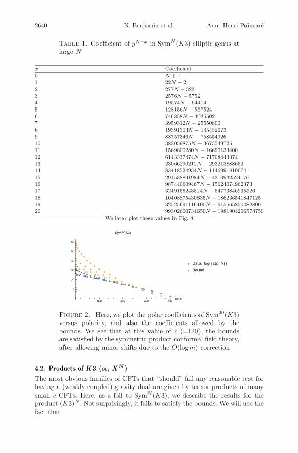
Table 1. Coefficient of yN−x in SymN (K3) elliptic genus atlarge N

x Coefficient

0 N + 11 22N − 22 277N − 3233 2576N − 57524 19574N − 644745 128156N − 5575246 746858N − 40355027 3959312N − 255508008 19391303N − 1454526739 88757346N − 75855492610 383059875N − 367354972511 1569800280N − 1669013340012 6143337474N − 7170844337413 23066290212N − 29321388865214 83418524934N − 114699181067415 291538891984N − 431093252417616 987440609467N − 1562407496237317 3249156243514N − 5477384693552618 10408875430635N − 18623654184712519 32525691116400N − 61556585048280020 99302600734650N − 1981904206578750

We later plot these values in Fig. 8

Figure 2. Here, we plot the polar coefficients of Sym20(K3)versus polarity, and also the coefficients allowed by thebounds. We see that at this value of c (=120), the boundsare satisfied by the symmetric product conformal field theory,after allowing minor shifts due to the O(log m) correction

4.2. Products of K3 (or, XN )

The most obvious families of CFTs that “should” fail any reasonable test forhaving a (weakly coupled) gravity dual are given by tensor products of manysmall c CFTs. Here, as a foil to SymN (K3), we describe the results for theproduct (K3)N . Not surprisingly, it fails to satisfy the bounds. We will use thefact that

Vol. 17 (2016) Elliptic Genera and 3d Gravity 2641

Figure 3. Here, we plot the polar coefficients of the productconformal field theory with target K320

Z(X⊗N )R,R (τ, z) =

(ZX

R,R(τ, z))N =

⎛⎝∑

n,�

cX(n, �)qny�

⎞⎠

N

. (4.10)

For concreteness, we look at the χy genus of K3N . Since

Z(K3)R,R (τ, z) = 2y−1 + 20 + 2y + O(q), (4.11)

the q0yN term in the elliptic genus of K3N is given by

cK3N (0, N) = 2N , (4.12)

which violates the bound (3.32) of only polynomial growth for the most polarterm.

To visualize the violation we plot the polar coefficients of K320 againstthe bound in Fig. 3. Note that the violations are not of the order O(log N),and (3.32) is clearly not satisfied.

We conclude with a few remarks about examples similar to the above:

1. We cannot rule out all product manifolds using this method. For in-stance, the elliptic genus of T 4 is zero, which means that products ofT 4 will surely satisfy the bound, having a vanishing elliptic genus. Thevanishing is due to cancellations arising from the U(1)4 translation sym-metry acting on SymN (T 4). One could instead work with SymN (T 4)/T 4.In worldsheet terms, there are fermion zero modes due to the extra trans-lation symmetry which must be saturated by the insertion of a suitablenumber of fermion currents. The relevant modification of the genus isworked out in [28]. It should be fairly straightforward to generalize ourconsiderations to situations such as this where extra insertions are re-quired to define a proper index.

2. Another simple example that violates the bound is the iterated symmetricproduct SymN1(SymN2(K3)). Taking, for simplicity, N1 = N2 = N , som = N2, the coefficient of the most polar term is

(2NN

)∼ 1√

πN4N =

1π1/2m1/4 4

√m for large m. Indeed, the iterated symmetric product is an

example of the more general class of permutation orbifolds. It would

2642 N. Benjamin et al. Ann. Henri Poincare

be interesting to explore the relation of our bound to the oligomorphiccriterion of [29,30].

4.3. Calabi–Yau Spaces of High Dimension

To provide a slightly more nontrivial test, we discuss the elliptic genera ofCalabi–Yau sigma models with target spaces X(d) given by the hypersurfacesof degree d + 2 in CP

d+1, e.g.,d+1∑i=0

zd+2i = 0. (4.13)

We have chosen these as the simplest representatives among Calabi–Yau man-ifolds of dimension d; as they are not expected to have any particularly specialproperty uniformly with dimension, we suspect this choice is more or lessrepresentative of the results we could obtain by surveying a richer class ofCalabi–Yau manifolds at each d. In any case we will settle with one Calabi–Yau per complex dimension. Since m = d/2, and we have been assuming m isintegral, we restrict to even d.

The elliptic genus for these spaces is independent of moduli, and can beconveniently computed in the Landau–Ginzburg orbifold phase. This yieldsthe formula [11]

ZdR,R(τ, z) =

1d + 2

d+1∑k,�=0

y−�

⎛⎝θ1

(τ,−d+1

d+2z + �d+2τ + k

d+2

)

θ1

(τ, 1

d+2z + �d+2τ + k

d+2

)⎞⎠

d+2

(4.14)

Many further facts about elliptic genera of Calabi–Yau spaces can be found in[31].

First, we discuss the explicit data. To facilitate this we computed allpolar coefficients numerically for d = 2, 4, . . . , 36. Then, we provide a simpleanalytical proof of bound violation valid for all values of d (just following fromthe behavior of the subleading polar term).

Using (4.14) we can extract the polar coefficients explicitly for any givend. In Figs. 4, 5, and 6 we plot the coefficients of the polar pieces againstpolarity for Calabi–Yau 10-, 20-, and 36-fold, respectively. In Fig. 7, we plotthe subleading polar coefficients of these Calabi–Yau spaces as a function oftheir dimension. In all cases, we see that the bounds are badly violated.

Numerics aside, it is easy to give a simple analytical argument provingthat these Calabi–Yaus will violate the bound. Consider the subleading ym−1

polar piece of Zd=2mRR .

The coefficients cX(d)(0, p) of the elliptic genera of Calabi–Yau spaces aredetermined simply by topological invariants:

cX(d)(0,m − i) =∑

k

(−1)i+khk,i, (4.15)

so the coefficient in front of ym−1 is

− χ1 =∑

p

−(−1)ph1,p. (4.16)

Vol. 17 (2016) Elliptic Genera and 3d Gravity 2643

Figure 4. Here, we plot the polar coefficients of Zd=10RR

Figure 5. Here, we plot the polar coefficients of Zd=20RR

Figure 6. Here, we plot the polar coefficients of Zd=36RR

We know h1,d−1 is given by the number of complex structure parameters ofthe hypersurface, or

h1,d−1 =(d + 2) × (d + 3) × · · · × (2d + 3)

1 × 2 × · · · × (d + 2)− (d + 2)2

=(

2d + 3d + 2

)− (d + 2)2. (4.17)

2644 N. Benjamin et al. Ann. Henri Poincare

Figure 7. Here, we plot the subleading polar coefficients ofthe Calabi–Yau elliptic genera against the dimension

By a standard application of the Lefschetz hyperplane theorem, the remainingh1,p vanish except for h1,1 = 1. Thus we get (recall d = 2m is even)

cX(d)(0,m − 1) =(

2d + 3d + 2

)− (d + 2)2 + 1. (4.18)

And just as a check, for d = 36, we numerically get

cX(36)(0, 17) = 3446310324346630675857

=(

7538

)− 382 + 1, (4.19)

which matches the expectation on the nose.Asymptotically, (4.18) goes as:

log cX(d)(0,m − 1) ∼ log (2d)! − 2 log (d)!

∼ 2d log (2d) − 2d log (d)

= 2d log 2 (4.20)

socX(d)(0,m − 1) ∼ 22d = 24m. (4.21)

To satisfy the bound, we need c(d)X (0,m − 1) to grow at most polynomially

with m when it in fact grows exponentially with m.

4.4. Enter the Monster

We now discuss a theory which passes our bounds but seemingly exhibitsno supergravity regime—instead exhibiting a Hagedorn degeneracy of statesalready at low energies. We have benefited immensely in thinking about thistheory from the unpublished work of Yin.

A c = 24 CFT with Monster symmetry was constructed many yearsago by Frenkel, Lepowsky, and Meurman [32]. Let us call the non-chiral CFTwith Monster symmetry M. In this section, we wish to consider the symmetricproducts SymN (M). As M has no moduli, there is a unique partition function

Vol. 17 (2016) Elliptic Genera and 3d Gravity 2645

canonically associated with this theory, and we will consider the chiral partitionfunction instead of the elliptic genus in this section.

This requires a word of explanation. While the elliptic genera we’ve con-sidered are related to non-chiral CFTs with conventional AdS gravity duals (infavorable cases), a chiral CFT can never have a conventional Einstein gravitydual. However, as explained in [33,34], there are candidates for chiral gravityduals to holomorphic CFTs. See also [35] and references therein for a more de-tailed discussion on these theories. In this sense, we can consider the partitionfunctions which follow as (candidate) duals to (a suitably defined theory of)chiral gravity (coupled to suitable matter).

Using the formula for the second-quantized partition function [26], alongwith the famous denominator identity due to Borcherds [36]:∏

n>0,m∈Z

(1 − pnqm)c(nm) = p(J(σ) − J(τ)) (4.22)

where p = e2πiσ and q = e2πiτ and J(τ) = q−1 +∑∞

n=1 c(n)qn, one can writethe generating function:

∞∑N=0

e2πiNσZ(SymN (M); τ) =e−2πiσ

J(σ) − J(τ). (4.23)

For large Im(τ) the infinite sum only converges for Im(σ) > Im(τ), while forsmall Im(τ) the infinite sum only converges for Im(σ + 1

τ ) > 1. Choosing largeIm(τ) we can say that

Z(SymN (M); τ) =∮

dσe−2πi(N+1)σ

J(σ) − J(τ), (4.24)

where the contour is a circle at constant Im(σ) on the cylinder given by thequotient of the σ-plane by σ ∼ σ + 1 and we must assume Im(σ) > Im(τ).The contour integral can—at least naively—be evaluated by deforming thecontour to smaller values of Im(σ) approaching Im(σ) = 0. (We certainlycannot deform to large Im(σ) because of the exponential growth from theterm e−2πi(N+1)σ.) This deformation leads to residues from an infinite set ofsimple poles at σ = τ together with σ equal to all the modular images of τwithin the strip |Re(τ)| ≤ 1

2 . Using

12πi

∂

∂τJ(τ) = −E2

4(τ)E6(τ)η(τ)24

. (4.25)

This naive contour deformation yields:

Z(SymN (M); τ) = P2(q−N−1)η(τ)24

E4(τ)2E6(τ). (4.26)

Here, P2(q−N−1) is the weight 2 Poincare series of q−N−1.3

3 This Poincare series requires regularization, indicating the above contour deformation argu-ment is subtle. A standard procedure for obtaining a well-defined Poincare series is describedin detail in many places. See, for examples, Sect. 4 of [14] or Sect. 2 of [46]. As explained inthose references, the modular anomaly of the series P2(q−N−1) is expressed in terms of a

2646 N. Benjamin et al. Ann. Henri Poincare

BecauseP2(q−N−1) = q−N−1 + O(1) , (4.27)

all of the modes which provide the low-energy spectrum (i.e., the states whichare not black holes) are visible in the expansion of

F (τ) =η(τ)24

E4(τ)2E6(τ). (4.28)

It now follows from the fact that c/24 = N and the structure of P2

that we can find the modes at energies below the black hole bound just fromexpanding F . Writing

F (τ) =∞∑

n=1

anqn, (4.29)

a1 is the ground-state contribution and the higher ak count the excited statesvisible in the partition function (until one reaches the threshold to form blackholes).

One can extract the kth coefficient via the contour integral

ak =1

2πi

∮dτ

1qk+1

F (τ). (4.30)

As η(τ) has no poles, E4 has a simple zero at τ = e2πi3 with no other zeroes,

and E6 has a simple zero at τ = i with no other zeros, we can now evaluate(4.30) explicitly.

The pole at τ = i provides the dominant behavior of the integral fork � 1. One finds

ak ∼ e2πk η(i)24

E4(i)2E′6(i)

, (4.31)

and hence in the regime 1 � n � N = c24 , the SymN (M) theory has a

degeneracy of polar states governed by

an ∼ e2πn . (4.32)

One can view this as satisfying an analog of the bound (3.32) for chiralgravity. In harmony with this, the singularity of (4.23) at σ = τ and at σ =−1/τ should come from the N → ∞ limit of the partition functions, andthis strongly suggests that the partition functions Z(SymN (M); τ) exhibitthe expected Hawking–Page first-order transition (as indeed follows from thegeneral results of [24]), that is, the large N asymptotics at fixed pure imaginaryτ is given by:

Z(SymN (M); τ) ∼{

κ1Nκ2q−N (1 + O(N−1)) Im(τ) ≥ 1

κ1Nκ2 q−N (1 + O(N−1)) Im(τ) ≤ 1

(4.33)

where q := exp(−2πi/τ). Here κ1, κ2 are constants we have not attempted todetermine.

Footnote 3 continuedperiod of a weight zero cusp form. Since no such nonzero cusp form exists we conclude thatP2(q−N−1) is in fact modular, as is required by modularity of Z(SymN (M); τ).

Vol. 17 (2016) Elliptic Genera and 3d Gravity 2647

The growth (4.32) exhibits a Hagedorn spectrum, hinting that if thereis a holographically dual theory it must be a string theory with string scalecomparable to the AdS radius.

5. String Versus Supergravity Duals

We have just seen that some theories with a low-energy Hagedorn degeneracy

# of states at energy E ∼ e2πn, 1 � E � c

24(5.1)

still satisfy our bounds. This might indicate that such theories are low-energystring theories—there is no parametric separation of scales evident between theemergence of a Hagedorn degeneracy and some other set of low-energy modeswith well-defined asymptotics (which could serve as a proxy for supergravityKK modes).4

This is to be contrasted with the growth of states exhibited by a super-gravity theory in d spatial dimensions, in the regime where the supergravitymodes have wavelengths shorter than any scale set by the curvature. The grav-ity modes then behave, to leading approximation, like a gas of free particlesin d dimensions. The energy per unit volume scales as

E ∼ T d+1, (5.2)

while the entropy per unit volume scales as

s ∼ T d. (5.3)

Hence, in such a theory, one expects (simply from dimensional analysis) that

cE ∼ econst×Eα

, α ≡ d

d + 1(5.4)

in the regime dominated by supergravity modes. For instance, in the canonicalAdS5 × S5 solution of IIB supergravity, there is a supergravity regime withE

910 growth of the entropy as a function of energy [15].

For AdS3×S3×K3 compactifications where the K3 is much smaller thanthe S3, one would expect a 6d supergravity regime to occur at low energies. Wenow provide some simple analytical and numerical arguments demonstratingthat the growth is indeed sub-Hagedorn. Related discussions appear in [37,38].The naive “gas of particles” analogy discussed above, for polar terms, wouldsuggest a growth of econst×E5/6

. One can get slower growth, however, due tocancellations in the supergravity modes which contribute to the elliptic genus.We also note that at gstring � 1, there would be a regime of energies in thefull physical theory exhibiting a Hagedorn degeneracy of string states. Thesedo not, however, contribute in the elliptic genus.

4 Two subtleties could invalidate the considerations of this section. In one direction, can-cellations between terms in a partition function could lead to subexponential growth ofcoefficients when in fact the entropy grows exponentially. In the other direction, when con-sidering the entropy at finite volume it can happen that the entropy grows exponentiallywith energy, even though the theory is not a string theory. For an example, see Sect. 7 of[47].

2648 N. Benjamin et al. Ann. Henri Poincare

First, we provide an analytical argument demonstrating that there is arange in which the polar terms of the elliptic genus of SymN (K3) clearly hassubexponential growth (though we do not quantify beyond this). Taking (4.4)at y = 1, we get that the sum of all O(q0) coefficients of the EG of SymN (K3)is the Nth coefficient of

q

η(τ)24(5.5)

which goes ase4π

√N+O(log N). (5.6)

Since all of the O(q0) pieces of the EG of SymN (K3) are positive (which canbe shown from (4.4) for instance), each individual term must be smaller than(5.6). If we label the O(q0) states by E as above (we are interested in thegrowth in the NS sector, and the different powers of y at O(q0) in the R sectorgenus give states of different NS energy), we must have

aE < e4π√

N (5.7)

ThusaNα < e4π

√N (5.8)

for α < 1 which correspond to states parametrically below the Planck mass inthe NS sector as N → ∞. Relabeling gives us

aE < e4πE12α . (5.9)

We therefore find states parametrically lighter than the Planck mass with asubexponential growth of states. Note that there may be other states at thesame energy level that we neglect due to only considering O(q0) terms in theelliptic genus. However, as we expect the entropy to be a function of polarityup to small corrections, taking terms with positive powers of q into accountwould only multiply our expression in (5.9) by some polynomial factor withoutchanging the leading order.

Because we expect the only relevant scales (other than supergravity KKscales) to be the string scale and Planck scale, and we do not get stringy growthin this regime, we expect subexponential growth throughout the polar terms.We now provide further (weak) numerical evidence in favor of this hypothesis.We include a plot of the normalized coefficients of yN−x for x = 1, . . . 40 inthe large N limit in Fig. 8 (these numbers do not change past some N sincethey only involve twisted sectors of permutations of some fixed length).

These examples suggest a criterion that distinguishes between theorieswith low-energy Einstein gravity duals as opposed to low-energy string duals,with the usual qualifier that cancellation is possible in an index computation.Writing

cE ∼ econst×Eα

, 1 � E � c

24, (5.10)

theories with α < 1 are likely to have a range of scales at low energy wheresupergravity applies, while theories with α = 1 are evidently string theoriesalready at the scale set by the curvature. We note that similar issues have been

Vol. 17 (2016) Elliptic Genera and 3d Gravity 2649

Figure 8. Here, we plot the normalized coefficients of yN−x

terms in elliptic genus of SymN (K3) for x = 1, . . . 40 inthe large N limit. Note the subexponential growth in theplot. Numerical values for the first twenty terms are given inTable 1

discussed, in the context of the duality between AdS4 gravity and CFT3, inthe interesting paper [39].

6. Estimating the Volume of an Interesting Set of ModularForms

In this section, we use (3.32) to try and quantify a lower bound on the “frac-tion of large m superconformal field theories which may admit a gravity dual”.Our approach will be to ask: “How special is the class of weight zero, indexm Jacobi forms corresponding to such superconformal theories?” As we haveseen, thermodynamic arguments constrain the growth of the polar coefficientsprovided there is a physically reasonable gravitational dual, so the problemreduces to quantifying “what fraction” of all possible polar coefficients corre-sponds to the theories with gravitational duals.

Since the Jacobi form is completely determined by its polar coefficients,the map from CFTs to elliptic genera can be viewed as a map from the spaceof (0, 2) field theories to a subset E ⊂ Z

j(m). Now, there is a natural metricon the moduli spaces of conformal field theories, namely, the Zamolodchikovmetric [40]. The moduli space of such theories, with a fixed central chargec, is a union of connected components �αM(c)

α . It was suggested some timeago that, at least for the space of (2, 2) superconformal theories, the totalZamolodchikov volume of V (c) :=

∑α vol (M(c)

α ) should be finite. This wasbased on physical arguments [41,42]. For the case of components arising fromCalabi–Yau manifolds it has been shown that indeed vol (M(c)

α ) is finite. (See[43] and references therein for the mathematical work on this subject.) The

2650 N. Benjamin et al. Ann. Henri Poincare

finiteness of V (c) would allow us to define a measure on the space of (2, 2)theories of a fixed central charge and thereby to quantify statements of “howoften” a property is exhibited in a natural way. We will assume that V (c) is infact finite.5

Using the push-forward measure under the map to the polar coefficients ofelliptic genera we obtain a natural measure on the space E of polar coefficients.Unfortunately, our present state of knowledge of conformal field theory is tooprimitive to evaluate this measure in great detail, but to illustrate the idea,and some of the issues which will arise, we will sketch two toy computations.

For our first toy computation we consider the pushforward to a measureon Z+ for the absolute value of the extreme polar coefficient of the ellipticgenus. We denote this by

e(C) = |c(0,m; C)| (6.1)

for a (2, 2) CFT C with c = 6m.Now e is multiplicative on CFTs,

e(C1 × C2) = e(C1)e(C2). (6.2)

We would also like to say the same for the volumes:

vol (C1 × C2)?= vol (C1)vol (C2) (6.3)

but this is in general not the case. Here vol (C) denotes the volume of theconnected component of V (c) in which C lies. A simple counterexample isprovided by conformal field theories with toroidal target spaces. Nevertheless,for ensembles such as theories based on generic Calabi–Yau manifolds thevolume is multiplicative, because the relevant Hodge numbers are additive.We will refer to an ensemble of CFT’s for which (6.3) holds as a multiplicativeensemble and here we restrict attention to such ensembles. Extending ourdiscussion beyond multiplicative ensembles is an interesting, but potentiallydifficult, problem.

Given a multiplicative ensemble, let us say an N = (2, 2) CFT C is primeif it is not the product of two such theories C1 and C2 each with positive centralcharge. Let C(m,α) denote the distinct prime CFT’s of central charge c = 6m,with α = 1, . . . , fm. We expect fm to be finite, but this is not necessary forour construction, so long as the relevant products below converge. Denote theabsolute value of the extreme polar coefficient, and the Zamolodchikov volumeof C(m,α) by e(m,α), v(m,α), respectively. Then the Zamolodchikov volumevol(M) of theories of central charge c = 6M is determined from:

∞∏m=1

fm∏α=1

11 − v(m,α)qm

= 1 +∞∑

M=1

vol(M)qM . (6.4)

Similarly, we can write a generating function for the volume of the theorieswith a fixed extreme polar coefficient. We assume that e(m,α) = 0 in our

5 Friedan has proposed a mechanism by which such a probability distribution might in factbe dynamically generated from more fundamental principles [48,49].

Vol. 17 (2016) Elliptic Genera and 3d Gravity 2651

ensemble (thus excluding, for example, Calabi–Yau models with odd complexdimension) and form the generating function:

∞∏m=1

fm∏α=1

11 − v(m,α)e(m,α)−sqm

= 1 +∞∑

M=1

ξ(s;M)qM (6.5)

Then

ξ(s;M) =∞∑e=1

vol (e;M)es

(6.6)

and the measure for the extreme polar coefficient is

μ(e;M) :=vol (e;M)vol (M)

. (6.7)

In order to make this slightly more concrete, let us restrict even further tothe ensemble of (4, 4) theories generated by taking products of the symmetricproducts of K3 sigma models, such as(

Sym1(K3))n1 ×

(Sym2(K3)

)n2 × · · ·(Sym�(K3)

)n�

. (6.8)

We will call this the K3-ensemble and it is a multiplicative ensemble of CFT’s.In this ensemble the prime CFTs are simply the symmetric products Symn(K3).For Sym1(K3) the moduli space M1 is the famous double quotient

M1 = O(Γ)\O(4, 20; R)/O(4) × O(20) (6.9)

with Γ ∼= II4 ⊕ E8 ⊕ E8, while for N > 1 the moduli space is [25,44,45]

MN = O(Γ′)\O(4, 21; R)/O(4) × O(21) (6.10)

with Γ′ a lattice of signature 4, 21 determined in [45]. The four “extra moduli”in (6.10) compared to (6.9) are due to the blowup multiplet at the locus of A1

singularities in SymN (K3) where two points meet. All higher twist fields areirrelevant. Denote the Zamolodchikov volume of these moduli spaces by vN .The Zamolodchikov volume vol(M) of the ensemble of models (6.8) is thensimply given by

∞∏n=1

11 − vnqn

= 1 +∞∑

M=1

vol(M)qM (6.11)

Now, to get the measure for a fixed extreme polar term we noted above that

e(Symn(K3)) = n + 1, (6.12)

so the extreme polar term of the elliptic genus of (6.8) is just the product:

2n13n2 . . . (� + 1)n� . (6.13)

Therefore, our general formula specializes to∞∏

m=1

11 − vm(m + 1)−sqm

= 1 +∞∑

M=1

ξ(s;M)qM , (6.14)

where ξ(s;M) defines the conditional volume as in (6.6) and the measure forthe extreme polar term is given by (6.7), above.

2652 N. Benjamin et al. Ann. Henri Poincare

Determining the numerical values of the constants vN used above is a veryinteresting problem in number theory. This will be discussed in a separatepaper, along with some applications of the function ξ(s;M) to the centralissue of this paper.6 It would also be very interesting to extend the abovediscussion to the ensemble of all (4, 4) theories, but this looks quite challenging.We would need to include products with SymN (T 4)/T 4. Moreover, we haveomitted products with other (4, 4) models constructable from permutationorbifolds, or from other compact hyperkahler manifolds arising from modulispaces of hyperholomorphic bundles on K3 and T 4. And we have omittedthe unknown unknowns since we do not know that every (4, 4) model can berealized geometrically. Nevertheless, we expect some of the basic features ofthe above discussion to survive better knowledge of the moduli space.

The above discussion is our first toy computation. Given our poor knowl-edge of the moduli space of conformal field theories we will resort to a sec-ond toy computation. We hope it proves instructive. We enumerate the po-lar coefficients c(a) by decreasing discriminant D(a) = �(a)2 − 4mn(a), a =0, . . . , j(m) − 1 where j(m) = dim J0,m. Thus, D(0) = m2. The idea of thesecond toy computation is to find a natural probability measure on the vectorspace of polar coefficients (c(0), . . . , c(N)). Of course, a vector space has infi-nite measure in its Euclidean norm so we map these coefficients to an affinecoordinate patch of RP

N , with N = j(m). That is, we consider the points[1 : c(0) : . . . : c(N)] in RP

N . We then consider the Fubini-Study measure onthis patch. Whether this measure bears any relation to the a priori Zamolod-chikov measure (in the large N limit) remains to be seen. (Since we do notlike the answer, we suspect the answer is that it does not.)

The volume element for the unit radius RPN in affine coordinates [1 :

ξ1 : . . . : ξN ] is:

dvol =dξ1 ∧ · · · ∧ dξN

(1 +∑

a(ξa)2)(N+1)/2. (6.15)

Now we consider the subspace of the affine coordinate patch with

|c(a)| ≤ R(a). (6.16)

R(a) is a bound which is supposed to come from physics. One reasonable guessis

R(a) = e2π(n(a)− |�(a)|2 + m

2 ). (6.17)

Note that this is imposing (3.32) without allowing an O(log m) correction.Concretely, we are interested in the fraction

fN =Γ(N+1

2 )

πN+1

2

⎛⎝ N∏

i=1

∫ e2π(ni− |�i|2 + m

2 )

−e2π(ni− |�i|2 + m

2 )dξi

⎞⎠ 1

(1 +∑

i(ξi)2)N+1

2

(6.18)

in the limit N → ∞.

6 For further details, see https://www.perimeterinstitute.ca/video-library/collection/mock-modularity-moonshine-and-string-theory.

Vol. 17 (2016) Elliptic Genera and 3d Gravity 2653

In Appendix B, we show that in the limit of large N ,

0.9699 < fN < 0.9725. (6.19)

We actually view this as a good indication that the Fubini-Study measure isnot a good surrogate for the Zamolodchikov measure. On general grounds, oneactually expects theories with weakly coupled gravity duals (even characteriz-ing some small region of their moduli space) to be rare creatures.

In general CFTs, the number of excited states at large energies n growslike e2π

√c6n by the Cardy formula. Hence a measure which was based on “ex-

pecting” there to be a small number of states in that regime would clearlybe incorrect. While one cannot use Cardy’s result in the energy range char-acterizing polar coefficients, it seems suspicious that our measure “expects”the fewer polar coefficients—related to states with high energy, though belowthe black hole bound—to be close to 0. In fact, one might expect that in arandom SCFT, the polar coefficients typically grow fairly rapidly with decreas-ing polarity. In such a case, it would be more difficult for them to lie withinthe polydisc specified by our bounds. Finding a modified volume estimate (orattaching a plausible physical meaning to our present estimate) will have toremain a problem for the future.

Acknowledgements

We thank J. de Boer, A. Castro, E. Dyer, A.L. Fitzpatrick, D. Friedan, S. Har-rison, K. Jensen, C. Keller, S. Minwalla, D. Tong, S.P. Trivedi, E. Verlinde, R.Volpato, and X. Yin for interesting discussions. We thank D. Ramirez for helpwith sophisticated mathematical diagrams and C. Keller for useful commentson the draft. This work was initiated at the Aspen Center for Physics andwe thank the ACP for its hospitality and excellent working conditions. TheACP is supported by NSF Grant No. PHY-1066293. N.B. acknowledges thesupport of the Stanford Graduate Fellowship. N.M.P. acknowledges supportfrom an NSF Graduate Research Fellowship. S.K. is grateful to the 2014 IndianStrings Conference, IISER-Pune, the Tata Institute for Fundamental Research,and the Kavli Institute for Theoretical Physics at UC Santa Barbara for hos-pitality while thinking about the physics of this note. His work was supportedin part by National Science Foundation Grant PHY-0756174 and DOE Officeof Basic Energy Sciences contract DE-AC02-76SF00515. M.C. is grateful toCambridge, Case Western Reserve, and Stanford Universities and Max PlanckInstitut fur Mathematik for hospitality. The work of G.M. is supported by theDOE under Grant DOE-SC0010008 to Rutgers, and NSF Focused ResearchGroup award DMS-1160461.

Open Access. This article is distributed under the terms of the Creative Com-mons Attribution 4.0 International License (http://creativecommons.org/licenses/by/4.0/), which permits unrestricted use, distribution, and reproduction in anymedium, provided you give appropriate credit to the original author(s) and the

2654 N. Benjamin et al. Ann. Henri Poincare

source, provide a link to the Creative Commons license, and indicate if changeswere made.

Appendix A: Extended Phase Diagram

Here, we derive in detail the extended phase diagram depicted in Fig. 1. Thelogic of the argument can be summarized as follows. The expression of theelliptic genus as a regularized Poincare sum involves a sum over all co-primepairs of integers (c, d). For each such pair arising from the invariant group Γθ ofZNS,+, we will find that there is an (n, �) labeling a polar term in the ellipticgenus which can serve as the analogue of our ground state in the ground-state dominance condition. As a consequence, in each region in the tessellatedupper-half plane there is a single pair (c, d) labeling the saddle point whichdominates the gravitational path integral (CFT elliptic genus). Each phasetransition across the bold lines in Fig. 1 is then a modular copy of the one westudied in this paper.

The elliptic genus can be written in terms of its polar part as [14]

ZR,R(τ, z) =12

∑r∈Z/2mZ

Cr(0) θm,r(τ, z) +12

∑�∈Z,n≥0D(n,�)>0

limK→∞

∑(Γ∞\Γ)K

C�(D(n, �)) exp(

2πi(n

aτ + b

cτ + d+ �

z

cτ + d− m

cz2

cτ + d

))R

(2πiD(n, �)

4m c(cτ + d)

)

(A.1)

where the limit coset is given by

limK→∞

∑(Γ∞\Γ)K

:= limK→∞

∑0<c<K

−K2<d<K2

(c,d)=1

(A.2)

and R is the regularization factor

R(x) =2√π

∫ x

0

e−zz1/2dz = erf(√

x) − 2√

x

πe−x, (A.3)

where erf(z) = 2√π

∫ z

0e−t2dt denotes the error function.

As discussed in [13], §6, using the classic identities

aτ + b

cτ + d=

a

c− 1

c(cτ + d)12

τ + 1cτ + d

=12c

− d

21

c(cτ + d)+

12

1cτ + d

c(τ/2 + 1/2)2

cτ + d=

τ

4+

2c − d

4c+

14

c2 − 2cd + d2

c(cτ + d)

Vol. 17 (2016) Elliptic Genera and 3d Gravity 2655

and Im(− 1c(cτ+d) ) = Im(τ)

|cτ+d|2 = Im(aτ+bcτ+d ), we see that

ZNS,+(τ) = (−1)mqm4

12

∑r∈Z/2mZ

Cr(0) θm,r

(τ,

τ + 12

)

+12

∑�∈Z,n≥0D(n,�)>0

limK→∞

∑(Γ∞\Γ)K

X(n, �; c, d)R(

2πiD(n, �)4mc(cτ + d)

)(A.4)

with∣∣∣X(n, �; c, d)∣∣∣

= |C�(D(n, �))| exp(

−2π Im(

aτ + b

cτ + d

) (m

(d − c)2

4+ n + �

d − c

2

)).

(A.5)

We would like to know which term in the elliptic genus, i.e., which pair(n, �), contributes the most to the sum in (A.1) with a given pair (c, d).First, focusing on the exponential factor in (A.5), using that Im

(aτ+bcτ+d

)> 0

and 0 < D(n, �) ≤ m2 we conclude that the maximum ofexp

(−2π Im

(aτ+bcτ+d

) (m (d−c)2

4 + n + � (d−c)2

))occurs at (n, �) = (nc,d, �c,d),

(nc,d, �c,d) := ( m4 ((d − c)2 − 1),−m(d − c))

when d − c is odd. Ignoring the other factors for the moment, we expect that∣∣∣X(n, �; c, d)∣∣∣ has its maximum

∣∣∣X(nc,d, �c,d; c, d

)∣∣∣ = C−m(m2) exp(

2πm

4Im

(aτ + b

cτ + d

))(A.6)

when (n, �) = (nc,d, �c,d). In the above we have used the fact that c(nc,d, �c,d)= c(0,m) = C−m(m2) is equal to the number of NS ground states [see (2.11)].

The situation is different for the pair of co-primes integers (c, d) witheven d − c. Using the more refined condition for the discriminants of the polarterms

0 < D(n, �) ≤ r2 where − m < r ≤ m, � = r mod 2m

that holds for all weak Jacobi forms as a straightforward consequence of (2.13),we see that the maximum of the exponential term in (A.5) is of order 1 whichis achieved whenever � = −(d − c)m + r, n = m(d − c)2 − (d−c)r

2 for any−m < r ≤ m. In other words, the contribution of the part of the sum givenby a pair (c, d) with c − d ≡ 0 (mod 2) in (A.1) is exponentially suppressed.

As a result, assuming that the exponential factor in (A.6) is the dominat-ing factor and ignoring for the moment the regularization factor, one concludesthat in each region in the upper-half plane given by the tessellation by Γ∞\Γθ

there is a unique pair (c, d) that dominates and this corresponds to the infin-itely many phases of 3d quantum gravity. To see this, notice that

Im(

aτ + b

cτ + d

)=

Im(τ)|cτ + d|2 ≤ Im(τ) ∀

(a bc d

)∈ Γθ

2656 N. Benjamin et al. Ann. Henri Poincare

whenever τ ∈ Γ∞F is in the (interior of the) fundamental domain

F = {τ ∈ H||τ | > 1, −1 < Re(τ) < 1}of Γθ or any of its images under the translation τ → τ +2n, n ∈ Z. See Fig. 1.

Next we would like to discuss the conditions under which that the termwith (n, �) = (nc,d, �c,d) indeed dominates the sum over all polar terms for agiven pair (c, d). First we show that the effect of the regularization factor can beignored at the large central charge limit where D(nc,d, �c,d)/4m = m/4 � 1.To see this, note that R(x) → 0 as x → 0 and

R(x) − 1 = O(√

x e−x)

as x → ∞, and

Re(

2πiD(n, �)4mc(cτ + d)

)=

2πD(n, �)4m

Im(

aτ + b

cτ + d

).

Second, for there to be no term over dominating the term coming from (n, �) =(nc,d, �c,d) in the sum in the region where aτ+b

cτ+d ∈ Γ∞F as predicted by analyz-ing the exponential factor alone as in (A.5), focussing on the line Re(aτ+b

cτ+d ) = 0we see that the coefficients of the polar terms have to satisfy

log |c(nc,d, �c,d)| ≤(

2π(m((d − c)2 + 1)

4+ n +

�(d − c)2

))

+ O(log m) (A.7)

for all co-prime pairs (c, d) with d − c odd. It is not hard to show that theseemingly stronger condition (A.7) is in fact implied by our bound (3.37) whentaking the spectral flow symmetry into account. Recalling that c(nc,d, �c,d) =C−m(m2) and

c(n, �) = c(n(k), �(k)) , n(k) = n + k2m + k�, �(k) = � + 2km

for all k ∈ Z, we can write (A.7) as

log |c(n(k), �(k))| ≤ 2π

(n(k) − |�(k)|

2+

m

2

)+ O(log m)

where k = d−c−12 .

In summary, we have proved the following. The condition (A.7) is re-quired for ZNS,+(τ) to be consistent with the phase structure given by thegroup Γ∞\Γθ (corresponding to distinct Euclidean BTZ black holes whichdominate in different regions of parameter space [23], §7.3). We have seen thatthe necessary condition (3.37) that we derived earlier in the paper, governingthe Hawking–Page transition, is sufficient to guarantee (A.7), and hence thefull expected phase diagram.

Appendix B: Estimating the Volumes of Regions in RPN

Recall the problem we have. We would like to estimate

fN =Γ(N+1

2 )

πN+1

2

⎛⎝ N∏

i=1

∫ e2π(ni− |�i|2 + m

2 )

−e2π(ni− |�i|2 + m

2 )dξi

⎞⎠ 1

(1 +∑

i(ξi)2)N+1

2

(B.1)

Vol. 17 (2016) Elliptic Genera and 3d Gravity 2657

Table 2. Most polar terms at index m (excluding ym)

Term e2π(n− |�|2 + m

2 )

ym−1 eπ

ym−2 e2π

qym e2π

ym−3 e3π

qym−1 e3π

ym−4 e4π

qym−2 e4π

q2ym e4π

ym−5 e5π

qym−3 e5π

q2ym−1 e5π

in the large N limit where N +1 is the number of polar terms of a Jacobi formof index m.

As an example, let us consider m = 2. We will later switch to the largem limit. There are only two polar terms: y2 and y1 so N = 1. We normalizethe y2 coefficient to 1, and the coefficient for y1 parametrizes RP

1 (the “pointat infinity” corresponds to a y2 coefficient of 0, but this has measure zero).

For y1, � = 1 and n = 0, so

e2π

(ni− |�i|

2 + m2

)= eπ. (B.2)

Thus the integral is

f2 =Γ(1)π

∫ eπ

−eπ

dξ11

(1 + ξ21)1

= 0.9725. (B.3)

In the large m limit, there are k+12 � integrals with limits −ekπ to ekπ (see

Table 2).

Appendix B.1: An Upper Bound

In this section, we will derive an upper bound on fN of 0.9725. Recall thefamous fact of life that

Γ(N+22 )

πN+2

2

∫ ∞

−∞dξN+1

1

(1 + ξ21 + · · · + ξ2

N+1)N+2

2

=Γ(N+1

2 )

πN+1

2

1

(1 + ξ21 + · · · + ξ2

N )N+1

2

. (B.4)

Thus, we can always take extra integrals to ∞ and we will get a strictly biggervalue. No matter how big N is, we will always have an integral with limits

2658 N. Benjamin et al. Ann. Henri Poincare

−eπ to eπ (coming from the ym−1 term). In particular

fN =Γ(N+1

2 )

πN+1

2

∫ eπ

−eπ

dξ1

∫dξ2 . . .

∫dξN

1

(1 + ξ21 + · · · + ξ2

N )N+1

2

<Γ(N+1

2 )

πN+1

2

∫ eπ

−eπ

dξ1

∫ ∞

−∞dξ2 . . .

∫ ∞

−∞dξN

1

(1 + ξ21 + · · · + ξ2

N )N+1

2

=1π

∫ eπ

−eπ

dξ11

1 + ξ21

= 0.9725, (B.5)

where we define an integral dξi with unlabeled limits as from −e2π(ni− |�i|2 + m

2 )

to e2π(ni− |�i|2 + m

2 ).

Appendix B.2: A Lower Bound

Now we will show a lower bound of 0.9699 through a series of inequalities.Again we use the same convention of unlabeled limits of integration dξi being

from −e2π(ni− �2i4m + m

4 ) to e2π(ni− �2i4m + m

4 ).First we will show

fN =Γ(N+1

2 )

πN+1

2

∫dξ1

∫dξ2 . . .

∫dξN

1

(1 + ξ21 + · · · + ξ2

N )N+1

2

> 1 −N∑

i=1

(1 − 1

π

∫dξi

11 + ξ2

i

). (B.6)

To see this, first rewrite (B.6) as

1 −Γ(N+1

2 )

πN+1

2

∫dξ1

∫dξ2 . . .

∫dξN

1

(1 + ξ21 + · · · + ξ2

N )N+1

2

<

N∑i=1

(1 − 1

π

∫dξi

11 + ξ2

i

). (B.7)

Now note that1π

∫dξi

11 + ξ2

i

(B.8)

represents the fraction of RPN where ξi is between the appropriate limits of

−e2π(ni− |�i|2 + m

2 ) to e2π(ni− |�i|2 + m

2 ). We write this as a fraction of RPN instead

of RP1 by using (B.4) to add the remaining N − 1 integrals from −∞ to ∞

and change the prefactor.In more detail, let us take the first term (i = 1) in the sum in the right-

hand side of (B.7). That term is

1 − 1π

∫ eπ

−eπ

dξ11

1 + ξ21

= 1 −Γ(N+1

2 )

πN+1

2

∫ eπ

−eπ

dξ1

∫ ∞

−∞dξ2 . . .

∫ ∞

−∞dξN

1

(1 + ξ21 + · · · + ξ2

N )N+1

2

(B.9)

Vol. 17 (2016) Elliptic Genera and 3d Gravity 2659

which is exactly the region outside −eπ < ξ1 < eπ in RPN . However, the

left-hand side of (B.7) is RPN with the region

|ξi| ≤ R(i), ∀ i

excluded.Thus, (B.7) is satisfied by using the fact that the complement of the

intersection is less than the sum of complements.Now we are in business. It is another classic fact of life that

1π

∫ R(i)

−R(i)

dξi1

1 + ξ2i

=2π

arctan R(i)

= 1 − 2πR(i)

+ · · · (B.10)

Plug into (B.6), to get:

1 −N∑

i=1

(1 − 1

π

∫dξi

11 + ξ2

i

)> 1 −

N∑i=1

2πR(i)

(B.11)

In the large m limit, the first terms look like

1 −N∑

i=1

2πai

= 1 − 2π

(1eπ

+2

e2π+

2e3π

+3

e4π+

3e5π

+ · · ·)

> 1 − 2π

(1eπ

+2

e2π+

3e3π

+4

e4π+

5e5π

+ · · ·)

= 1 − 2π

(1

eπ(1 − 1eπ )2

)

= 0.9699. (B.12)

Thus, putting everything together, we get

fN > 0.9699. (B.13)

References

[1] Maldacena, J.M.: The large N limit of superconformal field theories and super-gravity. Adv. Theor. Math. Phys. 2, 231 (1998). arXiv:hep-th/9711200

[2] Hartman, T., Keller, C. A., Stoica, B.: Universal spectrum of 2d conformal fieldtheory in the large c limit. arXiv:1405.5137 [hep-th]

[3] Witten, E.: Anti-de Sitter space, thermal phase transition, and confinement ingauge theories. Adv. Theor. Math. Phys. 2, 505 (1998). arXiv:hep-th/9803131

[4] Hawking, S.W., Page, D.N.: Thermodynamics of black holes in anti-De Sitterspace. Commun. Math. Phys. 87, 577 (1983)

[5] Schellekens, A.N., Warner, N.P.: Anomalies and modular invariance in stringtheory. Phys. Lett. B 177, 317 (1986)

[6] Schellekens, A.N., Warner, N.P.: Anomaly cancellation and selfdual lat-tices. Phys. Lett. B 181, 339 (1986)

2660 N. Benjamin et al. Ann. Henri Poincare

[7] Pilch, K., Schellekens, A.N., Warner, N.P.: Path integral calculation of stringanomalies. Nucl. Phys. B 287, 362 (1987)

[8] Witten, E.: Elliptic genera and quantum field theory. Commun. Math.Phys. 109, 525 (1987)

[9] Eichler, M., Zagier, D.: The theory of Jacobi forms. Birkhauser, Boston (1985)

[10] Strominger, A., Vafa, C.: Microscopic origin of the Bekenstein-Hawking entropy.Phys. Lett. B 379, 99 (1996). arXiv:hep-th/9601029

[11] Kawai, T., Yamada, Y., Yang, S. K.: Elliptic genera and N =2 superconformalfield theory. Nucl. Phys. B 414, 191 (1994). arXiv:hep-th/9306096

[12] Gaberdiel, M.R., Gukov, S., Keller, C.A., Moore, G.W., Ooguri, H.: ExtremalN =(2,2) 2D conformal field theories and constraints of modularity. Commun.Number Theor. Phys. 2, 743 (2008), arXiv:0805.4216 [hep-th]

[13] Dijkgraaf, R., Maldacena, J.M., Moore, G.W., Verlinde, E.P.: A black hole fareytail. arXiv:hep-th/0005003

[14] Manschot, J., Moore, G.W.: A modern farey tail. Commun. Number Theor.Phys. 4, 103 (2010), arXiv:0712.0573 [hep-th]

[15] Aharony, O., Gubser, S. S., Maldacena, J.M., Ooguri, H., Oz, Y.: LargeN field theories, string theory and gravity. Phys. Rep. 323, 183 (2000).arXiv:hep-th/9905111

[16] Kraus, P., Larsen, F.: Partition functions and elliptic genera from supergravity.JHEP 0701, 002 (2007). arXiv:hep-th/0607138

[17] Kraus, P.: Lectures on black holes and the AdS(3)/CFT(2) correspondence. Lect.Notes Phys. 755, 193 (2008). arXiv:hep-th/0609074

[18] Banados, M., Teitelboim, C., Zanelli, J.: The black hole in three-dimensionalspace-time. Phys. Rev. Lett. 69, 1849 (1992). arXiv:hep-th/9204099

[19] Cvetic, M., Larsen, F.: Near horizon geometry of rotating black holes in five-dimensions. Nucl. Phys. B 531, 239 (1998). arXiv:hep-th/9805097

[20] de Boer, J., Denef, F., El-Showk, S., Messamah, I., Van den Bleeken, D.: Blackhole bound states in AdS(3) x S**2. JHEP 0811, 050 (2008). arXiv:0802.2257[hep-th]

[21] Bena, I., Chowdhury, B.D., de Boer, J., El-Showk, S., Shigemori, M.: moultingblack holes. JHEP 1203, 094 (2012). arXiv:1108.0411 [hep-th]

[22] Maldacena, J.M., Strominger, A.: AdS(3) black holes and a stringy exclusionprinciple. JHEP 9812, 005 (1998). arXiv:hep-th/9804085

[23] Maloney, A., Witten, E.: Quantum gravity partition functions in three dimen-sions. JHEP 1002, 029 (2010). arXiv:0712.0155 [hep-th]

[24] Keller, C.A.: Phase transitions in symmetric orbifold CFTs and universality.JHEP 1103, 114 (2011). [arXiv:1101.4937 [hep-th]

[25] Dijkgraaf, R.: Instanton strings and hyperKahler geometry. Nucl. Phys. B 543,545 (1999). arXiv:hep-th/9810210

[26] Dijkgraaf, R., Moore, G.W., Verlinde, E.P., Verlinde, H.L.: Elliptic genera ofsymmetric products and second quantized strings. Commun. Math. Phys. 185,197 (1997). arXiv:hep-th/9608096

[27] Manschot, J., Zapata Rolon, J.M.: The asymptotic profile of χy-genera of Hilbertschemes of points on K3 surfaces. Commun. Number Theor. Phys. 09, 413 (2015).arXiv:1411.1093 [math.AG]

Vol. 17 (2016) Elliptic Genera and 3d Gravity 2661

[28] Maldacena, J.M., G.W., Strominger, A.: Counting BPS black holes in toroidaltype II string theory. arXiv:hep-th/9903163

[29] Haehl, F.M., Rangamani, M.: Permutation orbifolds and holography.arXiv:1412.2759 [hep-th]

[30] Belin, A., Keller, C.A., Maloney, A.: String universality for permutation orb-ifolds. arXiv:1412.7159 [hep-th]

[31] Gritsenko, V.: Elliptic genus of Calabi-Yau manifolds and Jacobi and Siegelmodular forms. arXiv:math/9906190

[32] Frenkel, I., Lepowsky, J., Meurman, A.: Vertex operator algebras and the mon-ster, Pure and Applied Mathematics, vol. 134. Academic (1988), Boston, p. 508

[33] Li, W., Song, W., Strominger, A.: Chiral gravity in three dimensions. JHEP0804, 082 (2008). arXiv:0801.4566 [hep-th]

[34] Maloney, A., Song, W., Strominger, A.: Chiral gravity, log gravity and extremalCFT. Phys. Rev. D 81, 064007 (2010). arXiv:0903.4573 [hep-th]

[35] Skenderis, K., Taylor, M., Van Rees, B.C.: Topologically massive gravity and theAdS/CFT correspondence. JHEP 0909, 045 (2009). arXiv:0906.4926 [hep-th]

[36] Borcherds, R.E.: The monster Lie algebra. Adv. Math. 83, 30 (1990)

[37] de Boer, J.: Large N elliptic genus and AdS/CFT correspondence. JHEP 9905,017 (1999). arXiv:hep-th/9812240

[38] de Boer, J., El-Showk, S., Messamah, I., Van den Bleeken, D.: A bound on theentropy of supergravity? JHEP 1002, 062 (2010). arXiv:0906.0011 [hep-th]

[39] Minwalla, S., Narayan, P., Sharma, T., Umesh, V., Yin, X.: Supersymmet-ric states in large N Chern-Simons-Matter theories. JHEP 1202, 022 (2012).arXiv:1104.0680 [hep-th]

[40] Zamolodchikov, A.B.: Irreversibility of the flux of the renormalization group ina 2D field theory. JETP Lett. 43, 730 (1986)

[41] Horne, J.H., Moore, G.W.: Chaotic coupling constants. Nucl. Phys. B 432, 109(1994). arXiv:hep-th/9403058

[42] Douglas, M.R., Lu, Z.: Finiteness of volume of moduli spaces.arXiv:hep-th/0509224

[43] Douglas, M., Lu, Z.: On the geometry of moduli space of polarized Calabi-Yaumanifolds. arXiv:math/0603414 [math-dg]

[44] Giveon, A., Kutasov, D., Seiberg, N.: Comments on string theory on AdS(3).Adv. Theor. Math. Phys. 2, 733 (1998). arXiv:hep-th/9806194

[45] Seiberg, N., Witten, E.: The D1/D5 system and singular CFT. JHEP 9904, 017(1999). arXiv:hep-th/9903224

[46] Cheng, M.C.N., Duncan, J.F.R.: Rademacher sums and rademacher series.arXiv:1210.3066 [math.NT]

[47] Galakhov, D., Longhi, P., Mainiero, T., Moore, G.W., Neitzke, A.: Wild wallcrossing and BPS giants. JHEP 1311, 046 (2013). arXiv:1305.5454 [hep-th]

[48] Friedan, D.: A Tentative theory of large distance physics. JHEP 0310, 063 (2003).arXiv:hep-th/0204131

[49] Friedan, D.: Two talks on a tentative theory of large distance physics.arXiv:hep-th/0212268

2662 N. Benjamin et al. Ann. Henri Poincare

Nathan Benjamin, Shamit Kachru and Natalie M. PaquetteStanford Institute for Theoretical PhysicsStanford UniversityStanford, CA 94305, USAe-mail: nathansb@stanford.edu;skachru@stanford.edu;npaquett@stanford.edu

and

SLAC National Accelerator Laboratory2575 Sand Hill RoadMenlo Park, CA 94025, USA

Miranda C. N. ChengInstitute of Physics and Korteweg-de Vries Institute for MathematicsUniversity of AmsterdamAmsterdam, The Netherlandse-mail: mcheng@uva.nl

Gregory W. MooreNHETC and Department of Physics and AstronomyRutgers UniversityPiscataway, NJ 08855, USAe-mail: gmoore@physics.rutgers.edu

Communicated by Boris Pioline.

Received: July 8, 2015.

Accepted: December 7, 2015.