Embed Size (px)
Citation preview

Rochester Institute of Technology Rochester Institute of Technology
RIT Scholar Works RIT Scholar Works
Theses
2008
Elliptic curve cryptography: Generation and validation of domain Elliptic curve cryptography: Generation and validation of domain
parameters in binary Galois Fields parameters in binary Galois Fields
Peter Wozny
Follow this and additional works at: https://scholarworks.rit.edu/theses
Recommended Citation Recommended Citation Wozny, Peter, "Elliptic curve cryptography: Generation and validation of domain parameters in binary Galois Fields" (2008). Thesis. Rochester Institute of Technology. Accessed from
This Thesis is brought to you for free and open access by RIT Scholar Works. It has been accepted for inclusion in Theses by an authorized administrator of RIT Scholar Works. For more information, please contact [email protected].

_______________________________________________________________
Elliptic Curve Cryptography: Generation and Validation of Domain
Parameters in Binary Galois Fields _______________________________________________________________
Peter Wozny Department of Computer Science Rochester Institute of Technology
August 15, 2008
Committee Prof. Stanisław Radziszowski, Chairman
Prof. Christopher Homan, Reader Prof. Marcin Łukowiak, Observer

ii
MASTER OF SCIENCE THESIS
ROCHESTER INSTITUTE OF TECHNOLOGY DEPARTMENT OF COMPUTER SCIENCE
Elliptic Curve Cryptography:
Generation and Validation of Domain Parameters in Binary Galois Fields
____________________________________ Prof. Stanisław Radziszowski, Chairman
Department of Computer Science Rochester Institute of Technology
____________________________________ Prof. Christopher Homan, Reader Department of Computer Science Rochester Institute of Technology
____________________________________ Prof. Marcin Łukowiak, Observer
Department of Computer Engineering Rochester Institute of Technology
____________________________________ Approval Date

iii
Abstract
Elliptic curve cryptography (ECC) is an increasingly popular method for securing many forms of data and communication via public key encryption. The algorithm utilizes key parameters, referred to as the domain parameters. These parameters must adhere to specific characteristics in order to be valid for use in the algorithm. The American National Standards Institute (ANSI), in ANSI X9.62, provides the process for generating and validating these parameters. The National Institute of Standards and Technology (NIST) has identified fifteen sets of parameters; five for prime fields, five for binary fields, and five for Koblitz curves. The parameter generation and validation processes have several key issues. The first is the fast reduction within the proper modulus. The modulus chosen is an irreducible polynomial having degree greater than 160. Choosing irreducible polynomials of a particular order is less critical since they have isomorphic properties, mathematically. However, since there are differences in performance, there are standards that determine the specific polynomials chosen. The NIST standards are also based on word lengths of 32 bits. Processor architecture, primality, and validation of irreducibility are other important characteristics. The area of ECC that is researched is the generation and validation processes, as they are specified for binary Galois Fields F (2m). The rationale for the parameters, as computed for 32 bit and 64 bit computer architectures, and the algorithms used for implementation, as specified by ANSI, NIST and others, are examined. The methods for fast reduction are also examined as a baseline for understanding these parameters. Another aspect of the research is to determine a set of parameters beyond the 571-bit length that meet the necessary criteria as determined by the standards.

iv
Contents Abstract........................................................................................................ iii Introduction................................................................................................... 1 Fundamentals of Elliptic Curves.................................................................... 4
Basics of Elliptic Curves............................................................................ 5 Elliptic Curve Mathematics ....................................................................... 6 Polynomial and Normal Bases ..................................................................12
Basis Conversion ..................................................................................13 Koblitz Curves .........................................................................................14
Elliptic Curve Domain Parameters................................................................16 Identification of the Domain Parameters F (2m) ........................................17 Criteria for Domain Parameters ................................................................18 Federal Standards for Domain Parameters ................................................19 International Standards .............................................................................20
Domain Parameter Generation & Validation.................................................21 Algorithm for Generating Parameters .......................................................22 Verifiably Random Domain Parameters....................................................23 Determining the Order for the Elliptic Curve ............................................24
Point-Counting and Calculating Order ..................................................25 Primality Testing Algorithms................................................................27
Generating the Base Point.........................................................................28 Validating Domain Parameters .................................................................29
Selection Criteria for Parameter Generations ................................................31 Pseudo-Random Number Generation........................................................32 Security Level and Degree of the Field .....................................................32 32-bit Architecture ...................................................................................33 Selection of Basis .....................................................................................34
Fast reduction .......................................................................................34

v
Selection of Hash Algorithm.....................................................................35 Security Criteria .......................................................................................35
MOV Attack.........................................................................................35 Anomalous Condition...........................................................................36
Algorithms and Analysis ..............................................................................37 Algorithms ...............................................................................................38 Generating Elliptic Curve .........................................................................38 Computing the Order................................................................................39
Results and Conclusion ................................................................................41 Results of Implementation ........................................................................42 Results of Case Study ...............................................................................42 Summary..................................................................................................44
Criteria Synopsis ..................................................................................44 Future Work .............................................................................................45
Appendices...................................................................................................46 Appendix A – Abbreviations ....................................................................46 Appendix B – NIST Standards..................................................................47
Binary Field (2163) ................................................................................47 Binary Field (2233) ................................................................................47 Binary Field (2283) ................................................................................48 Binary Field (2409) ................................................................................49 Binary Field (2571) ................................................................................49
Appendix C – Irreducible Polynomials and Prime Numbers......................51 Appendix D – Almost Prime Koblitz Curve Orders ..................................55
Annotated Bibliography ...............................................................................57 Books .......................................................................................................57 Websites...................................................................................................57 Federal Publications / White Papers..........................................................58 Additional Publications ............................................................................59

vi
Figures Figure 1: ANSI X9.62 Protocol for Elliptic Curve Cryptography ................... 3 Figure 2: Elliptic Curve (y2 = x3-4x +2) ........................................................ 6 Figure 3: Point P and the Negative of P ........................................................ 7 Figure 4: Addition of Points P, Q .................................................................. 7 Figure 5: Points for: y2 = x3+ 1x + 7 (mod 139) .......................................... 8 Figure 6: Toroid of Points for: y2 = x3+ 1x + 7 (mod 139) ........................... 9 Figure 7: Toroid of Points for: y2 = x3+ 1x + 7 (mod 31)............................. 9 Figure 8: Domain Parameters for ECC (ANSI X9.62-1998)[37]...................17 Figure 9: Definition of Elliptic Curve Parameters (ANSI X9.62-2005)[22] ...18 Figure 10: Approved Security Level and Bound for the Order ......................19 Figure 11: Elliptic Curve Standard Sizes and the U.S. Standards Entity [24]19 Figure 12: Reduction Polynomials in Binary Galois Fields [22]...................20 Figure 13: Ways to Obtain the Domain Parameters .....................................22 Figure 14: Steps in Obtaining the Domain Parameters[22] ..........................23 Figure 15: Algorithm for Generating Verifiably Random Elliptic Curves[22]
.............................................................................................................24 Figure 16: Base Point Generation (ANSI X9.62-2005)[22]...........................29 Figure 17: Symmetric Key Length and Field Size Comparison[26] ...............32 Figure 18: ECC to RSA Key Length Comparison[4] .....................................33 Figure 19: Utilization of Other Existing Hash Functions..............................35

vii

1
Chapter 1 Introduction The purpose of this thesis is to examine the generation and validation of the domain parameters for elliptic curve cryptography (ECC), in particular as defined by National Institute of Standards and Technology (NIST) and the Institute of Electrical and Electronics Engineers (IEEE) standards, as well as by the American National Standards Institute (ANSI) and the Secure and Efficient Cryptography Group (SECG), for binary Galois fields. Conditions, such as primality, randomness, irreducibility, point counting, and fast reduction are essential characteristics of elliptic curve cryptography. The standard algorithms for generating and validating parameters are researched for implementation, after a thorough understanding of the processes associated for verifiably random parameters. The federal standards for elliptic curves, associated with cryptography, are rather difficult to understand and raise several questions. How are the domain parameters generated? Why are there only five set of parameters defined for binary Galois fields and five for Koblitz curves? What are all the essential criteria for choosing the domain parameters? Are there other useful parameters that are available that meet the necessary criteria? And, with

2
several published documents identifying the “standards,” then what is the real standard? Elliptic curves are denoted by specific points that statisfy the elliptic curve equations. Having a method to determining the number of valid points on an elliptic curve, in binary Galois fields, is important for understanding the level of difficulty an attacker would have in attempting to break ECC. It is also essential in computing the order of the elliptic curve. We implement an algorithm, similar to a Lucas sequence [8], which computes the number of points on Koblitz curves, determine which other field sizes could potentially be useful as a domain parameter. Since the testing of ECC must follow the Security Requirements for Cryptographic Modules, which is published by the U.S. Dept. of Commerce and NIST, these publications establish the criteria for security [35]. In addition, the ANSI standard [22] defines two security criteria, the MOV and Anomalous conditions. We examine how the domain parameters are affected and impacted by compliance to these conditions. More specifically, these conditions are stepped through for approved domain parameters to gain an understanding of the criteria necessary for new domain parameters generation. The U.S. Dept. of Commerce, Department of Commerce Security Requirements [33], notes that software based cryptography only meets level 1 security standards. Beyond level 1 security requires methods and techniques of securing hardware and encryption at the hardware level itself, and are not analyzed further during research. Lastly, a brief description of the criteria for a hash algorithm is described in order to understand what is necessary for an eventual replacement to the SHA-1 and SHA-2 hash algorithms [19]. In order to gain a clearer understanding of the elliptic curve algorithm, as it is used for digital signatures, several characteristics are identified. These characteristics include parameters and associations within the context of key generation, encryption, signatures and authentication, and the associated verifications. For this purpose, the ANSI X9.62 standards are a critical standard that provides the necessary information. The ANSI standard along with the NIST 186-2 and IEEE standards provide the global perspective, standards and federally accepted parameters for the ECC algorithm [22, 26, 35]. The ANSI X9.62 standard [22] describes the elliptic curve algorithm as it pertains to the following:
• Creating elliptic curve parameters

3
• Validation of the parameters • Key pair generation and validation • Signature generation and implementation • Authentication of the signature
The following graph (figure 1) describes the steps in the ECC process (as per ANSI X9.62).
Figure 1: ANSI X9.62 Protocol for Elliptic Curve Cryptography
Since the binary Galois fields, (F (2m)), are the most important due to their implementation with hardware and binary processing, their associated domain parameters for ECC are examined. This is a special case of the optimal extension field, (F (pm)), where the prime value p=2 [1]. The prime field case occurs when m=1. In the binary Galois field, the output can be given with respect to two particular bases, polynomial basis and the normal basis. FIPS 186-2 provides an algorithm for the conversion between the polynomial basis and the normal basis.
ECC Parameters
(NIST Standards)
Parameter Validation
Key Pair Generation
Public Key Validation
Digital Signature Generation
Message Digesting
Modular Computation
EC Computation
Validation of Signature
Digital Signature Validation / Authentication
Message Digesting
EC Computation
Modular Computation
Digital Signature

4
Chapter 2 Fundamentals of Elliptic Curves
• Basics of Elliptic Curves • Elliptic Curve Mathematics • Polynomial & Normal Basis • Koblitz Curves
5
Basics of Elliptic Curves Elliptic Curve Cryptography is a public key cryptographic system (PKCS) which utilizes points on elliptic curves. These points can be represented graphically in a two-dimensional plane, or a toroid [4, 6]. Elliptic curves are based on the following equation, known as the generic Weierstrass equation:
y2 + a1xy + a3y = x3 + a2x2 + a4x + a6 (1) The mathematics associated with ECC is performed in prime fields, binary fields, or optimal extended fields. Real numbers are used mainly for examples and understanding the fundamentals of the algorithm. Prime field and binary fields are specific conditions of the optimal extended field space [1]. Prime fields, denoted by F (p), utilizes the following variation of equation (1) to generate the necessary elliptic curve. y2 = x3+ ax + b mod (p); where 4a3 + 27b2 ≠ 0 (2) Binary field space, denoted by F (2m), utilizes the following variation of equation (1) to generate the associated elliptic curves.
y2 + xy = x3+ ax2 + b mod (2m); where b ≠ 0 (3) In addition to the specific equation for usage in binary fields, there is a normal and a polynomial basis that is utilized with a particular encryption method. For polynomial basis, field elements are reduced by the irreducible polynomial modulus. The modulus will be inferred, but not shown in following equations. There is a conversion algorithm that can convert from one basis to the other. In the process to generate the elliptic curves, encrypting and decrypting data, generating key pairs, signatures and authentication, several parameters are needed. These are the domain parameters. NIST, IEEE and ANSI provided the federally accepted standard parameters for ECC. These associated parameters are considerably smaller than those defined by the RSA algorithm, and ECC provides greater levels of security with less overhead. However, there is only a small sets of recommended values for the various fields. For the binary field, there are only five set of parameters specified by NIST as standards for various security levels of encryption, not including the five

6
associated for the Kolbitz curves [35]. These parameters have been chosen for fast reduction with their respective modulo [1]. Elliptic Curve Mathematics In order to understand the mathematics associated with elliptic curves, a preliminary examination of the Group Laws will be described as they apply to finite and infinite fields [6]. As stated earlier, the elliptic curve equation in prime fields is as follows:
y2 = x3+ ax + b; where 4a3 + 27b2 ≠ 0
Elliptic Curve Mathematics for Prime Fields Figure 2 shows a basic elliptic curve in a real field. It is used to emphasize the mathematical concepts. Points on an elliptic curve are governed by certain rules [6]. These are the following Group Laws.
Figure 2: Elliptic Curve (y2 = x3-4x +2)
1. P + ∞ = P where ∞ is the “infinity point.”
2. If P = (xP, yP), then (xP, yP) + (xP, - yP) = ∞ . (xP, - yP) = -P

7
Figure 3: Point P and the Negative of P
3. If P = (xP, yP) and Q = (xQ, yQ) with P ≠ -Q and P ≠ Q, then
R = P + Q = (xR, yR), given by: xR = λ2 - xP - xQ,, yR = λ(xP - xR) - yP
where
Figure 4: Addition of Points P, Q
4. For point doubling, if P = (xP, yP) then R = 2P = (xP, yP) + (xR, yR)
given by: xR = λ2 - 2xP, yR = λ(xP - xR) - yP
where
PQ
PQ
xx
yy
!
!="
!
3x p2
+a
2yP
!
" =
Example: For F (11) P = (1, 3) for elliptic curve: y2 = x3+ 1x + 7 (mod 11)
2P = (7, 4)

8
All of the viable points on an elliptic curve can be graphed in a two-dimensional plane, whose dimensions are p-1 by p-1. Viable points are those which solve the elliptic curve equation. Along with any set of points, the infinity point is also to be accounted for. Figure 5 shows the set of points, excluding (∞, ∞), for the elliptic curve:
y2 = x3+ 1x + 7 (mod 139)
Figure 5: Points for: y2 = x3+ 1x + 7 (mod 139)
These points can be represented not only in a two-dimensional plane, but since they are associated with a modulus, the plane can be seen as a toroid. The toroid is created by bringing the top and bottom edges together, and then similarly, bringing the right and left sides together. The end result is a toroid, as the one represented in Figure 6, showing all of the points on a partially transparent image. The points specified denote the (0, 0) position.

9
Figure 6: Toroid of Points for: y2 = x3+ 1x + 7 (mod 139)
Figure 7: Toroid of Points for: y2 = x3+ 1x + 7 (mod 31)
Figure 7 shows the point on the same elliptic curve taken with a different modulus. The mesh of the figure shows the two-dimensional characteristics of the plane as they were wrapped around to create the toroid. Elliptic Curve Mathematics for Binary Galois Fields The mathematics associated with elliptic curves is also performed using mathematic techniques that apply to binary fields (F (2m)) [6]. As stated earlier, the elliptic curve equation in binary field space is:
y2 + xy = x3+ ax + b; where b ≠ 0
The first three group laws are repeated for completeness, as associated with binary Galois fields. The details of point doubling are shown below.

10
Recalling: y2 + a1xy + a3y = x3 + a2x2 + a4x + a6 And for non-supersingular curves: a1 = 1, a2 = a, a3 = 0, a4 = 0, a6 = b
y2 + xy = x3 + ax2 + b
1. P + ∞ = P where ∞ is the “infinity point”
2. If P = (xP, yP), then (xP, yP) + (xP, - a1 xP - a3 - yP) = ∞ . -P = (xP, - a1 x - a3 - yP), or (xP, - xP - yP);
3. If P = (xP, yP) and Q = (xQ, yQ) with P ≠ -Q and P ≠ Q, then
R = -R’= (xR, yR), given by:
xR’ = λ2 - xP - xQ, yR’ = λ (xP - xR) + yP
where
and since xR = xR’
R= (xR , - xR - yR’).
4. Point Doubling Base Equation: y2 + xy = x3 + ax2 + b
Rearranging the equation: y2 + xy + x3 + ax2 + b = 0
By implicit differentiation:
!
" = slope =d
dx= y '
.02mod023)('2 2=!
"
#$%
&+++++ xxx
dx
dyy
dx
dxyy
PQ
PQ
xx
yy
!
!="
!
xy'+y + x2( ) = 0
!
y'= " =y + x
2
x
#
$ %
&
' (

11
A line through a point, P = (x0, y0), has the following y value:
By substitution, 0 = (λx+b)2 + x(λx+b) + x3 + a2x2 + a6 = x3 + (λ2+λ+a2 )x2 + … which is similar to the root of elliptic curve in F(p). So (x0 + x0 + x1) = ( λ2+λ+a2 )
Since
then
Doubling P0 = (x0, y0) gives P1 = (x1, y1) = -2P having the following values:
Therefore 2P = (x2, y2)
For binary Galois fields, using the generic Weierstrass equation, the negative of a point P, denoted by (xP, yP), is (xP, -a1xP-a3-yP) [6]. A solid understanding of the mathematics of elliptic curves is essential to understanding the generation of parameters associated with elliptic curve cryptography.
!
y = "(x # x0) + y
0= "x + b
!
x1
= "2 + " + a2
=y0
2+ x
0
4+ x
0y0
+ x0
3+ a
2x0
2
x0
2=x0
4+ a
6
x0
2.
!
y0
2= x
0y0
+ x0
3+ a
2x0
2+ a
6
!
y1
= "(x1# x
0) + y
0.
!
y1
= "(x1# x
0) + y
0.
!
x2
=x0
4+ a
6
x0
2,
!
y2
= "x1" y
1= x
1+ y
1.
!
x1
=x0
4+ a
6
x0
2,

12
Polynomial and Normal Bases There are two baselines for representing elliptic curve information and parameter data. They are polynomial basis and normal basis. The polynomial basis interprets each element of a binary Galois field as though it were a binary polynomial. They are represented as binary numbers, and each bit is the coefficient of a polynomial equation [35].
!
"(x) ="m#1x
m#1+"
m#2xm#2
+ ...+"1x1+"
0
The elements of the associated field, F (2m), are also held to the constraint that they are reduced by an irreducible polynomial, known as a reduction polynomial [1]. An irreducible polynomial is a polynomial that cannot be factored to anything other than 1 and itself. The reduction polynomial, f(x), is a polynomial whose highest degree is that of the field, m. This polynomial can be in two particular forms, trinomial or pentanomial [1].
!
f (x) = xm
+ xk
+1
!
f (x) = xm
+ xk3 + x
k2 + xk1 +1
The condition for the polynomial to be chosen as the designated irreducible polynomial of the associated degree is the following. The value m is the same as the degree of the field. For a trinomial, the value for k, is the smallest k that exists of the available irreducible polynomials of that degree. For the pentanomials, k3, is chosen as the smallest available k3 such that k3 >k2 >k1 [1]. For example, both of the following polynomials are of degree 8. However, the one denoted on the bottom is the irreducible polynomial, since it meets the criteria mentioned earlier. A listing of irreducible polynomials, of the type described above, trinomial and pentanomial, are provided in Appendix C, from FIPS 186-2 [35].
f(x) = x8 + x6 + x5 + x + 1 [2]
f(x) = x8 + x4 + x3 + x + 1 [1]

13
Normal basis elements are represented a little differently. They have the advantage in implementation of squaring. This mathematical function is applied efficiently [22]. They have the following form.
!
N = {"," 2," 2
2
,...," 2m#1
} and
!
{" # F(2m)}
Deciding upon a basis to use is not essential, as long as it is consistent, and that the recipient of the parameters knows what the basis is. The reason for this is that the basis have conversions associated with them. One can switch from a normal basis to a polynomial basis, and vice versa by means of a conversion matrix. Each conversion matrix is based on the degree of the field. The matrix is an m-by-m matrix whose rows are calculated with the modulus of the reduction polynomial [26].
Basis Conversion An essential component of elliptic curve parameter generation is the ability to convert elements from one basis to another. This is done by means of a conversion matrix [22, 26, 35]. A conversion matrix, Γ1, is an m-by-m matrix composed of {0, 1}. NIST provides a row, β, for the conversion matrix associated for the five standards. Subsequent rows are easily calculated within the given modulus, the modulus being the irreducible polynomial [35]. Conversion from a normal basis to polynomial basis is calculated by matrix multiplication, denoted as follows:
!
n " #1
= p where n is the bit-string of the normal basis element, and p is the resulting polynomial basis representation of the normal element. Γ1 is constructed by a series of squaring and reduction algorithms. Starting with theβ, each following row’s values are obtained by squaring the previous row and reducing by the irreducible polynomial [26].

14
!!!!!
"
#
$$$$$
%
&
=
!!!!
"
#
$$$$
%
&
='
(
((((
(
(
)(mod
)(mod
)(mod
...
...
...
12
2
1
1,11,10,1
1,11,10,1
1,01,00,0
1
xp
xp
xp
m
mmmm
m
m
)
)
)
)))
)))
)))
MMOMM
Conversion from a polynomial basis to normal basis is calculated also by matrix multiplication, denoted as follows:
!
p " #2
= n However, the input bit-string is in reverse sequential order. The highest order bit is on the right, and the lowest order bit is on the left. The conversion matrix is the inverse of the normal-to-polynomial conversion matrix. NIST provides the second-to-last row of the conversion matrix [26].
!
"2 =
#m$1mod p(x)
#m$2mod p(x)
M
#1mod p(x)
# 0 =1
%
&
' ' ' ' ' '
(
)
* * * * * *
In both cases, the result is an m length bit-string representing the input element in the opposite basis. Unlike simply finding the value for β, computing β and the conversion matrix for an arbitrarily chosen field requires several steps. These steps utilize matrix manipulations with a modulus, which is a specified irreducible polynomial. [22] Koblitz Curves The general elliptic curve equation for binary Galois fields is of the form:
y2 + xy = x3+ ax + b; where b ≠ 0. The equation for Koblitz curve takes on one of the following forms:

15
y2 + xy = x3+ x2 + 1
y2 + xy = x3 + 1
Koblitz curves, which are also known as anomalous binary curves [1], provide an efficient means for implementation and computation, especially with respect to multiplication. Point doubling employs the usual means by which multiplication is performed. However, with Kobitz curves, there is no special point doubling. Computing the order for Koblitz curves is calculated very quickly. The order is valid only for certain prime values associated with the degree of the field. This will be examined further in Chapter 4 of this document.

16
Chapter 3 Elliptic Curve Domain Parameters
• Identification of the Domain Parameters in F (2m) • Criteria for Domain Parameters • Federal Standards for Domain Parameters
o IEEE P1363 o NIST FIPS 186-2 o ANSI X9.62-2005
• International Standards o ISO / IEC and the SECG

17
Identification of the Domain Parameters F (2m) An elliptic curve has several parameters associated with it so as to define it. Points on an elliptic curve also are characteristic of a particular elliptic curve. Federal standards dictate what the associated domain parameters are for specific elliptic curves. Those standards allow for simplified implementation of elliptic curve standards for cryptography and signatures (ECDSA), without having to create a new set of parameters which must be validated. The parameters that are used in F (2m) are specified in several important published standards, such as ANSI X9.62, NIST FIPS 186-2, and SECG-2. The following is extracted from X9.62-1998 [37]. These descriptions of parameters are also valid in X9.62-2005 [22]. However, the current ANSI standard denotes that parameters, which complied with the old standard, are considered invalid under the new standard.
Figure 8: Domain Parameters for ECC (ANSI X9.62-1998)[37]
5.1.2.1 Elliptic curve domain parameters over F(2m)
Elliptic curve domain parameters over F(2m)shall consist of the following
parameters: 1. A field size q=2m which defines the underlying finite field F q, an indication
of the basis used to represent the elements of the field (TPB, PPB or GNB), and a reduction polynomial of degree m over F 2 if the basis used is a TPB or PPB;
2. (Optional) A bit string SEED of length at least 160 bits, if the elliptic curve was randomly generated in accordance with Annex A.3.3;
3. Two field elements a and b in F q which define the equation of the elliptic curve E:
y2 + xy = x3+ ax + b; 4. Two field elements xG and yG in F q which define a point G = (xG, yG) of
prime order on E (note G ≠ O); 5. The order n of the point G (it must be the case than n>2160 and n>4√q); and 6. (Optional) The cofactor h = #E(F q)/n. Annex A.3.2 specifies the method that shall be used for generating an elliptic
curve E over F q and the point G of order n.

18
Figure 9: Definition of Elliptic Curve Parameters (ANSI X9.62-2005)[22] Therefore, for binary Galois fields, where an elliptic curve is defined as:
E : y2 + xy = x3 + ax2 + b. The parameters that are needed are the following [1]:
1. m = field size and power or the leading x of the irreducible polynomial
2. f(x) = irreducible polynomial modulus for polynomial basis 3. a = coefficient for the elliptic curve equation 4. b = coefficient for the elliptic curve equation 5. P = (xp, yp), a point on the elliptic curve 6. n = the order of the point, P 7. h = the cofactor, such that h = #E(F (2m) )/ n
h ∈ { 2, 4 } 8. s = seed for the hash function for random parameter generation
Criteria for Domain Parameters Domain parameters are chosen based on certain security and performance criteria. These criteria are based on the needs of the encryption (the level chosen), and the types of possible attacks that can be instigated on an elliptic curve cryptosystem. These attacks, the MOV and Anomalous attacks will be discussed [22, 35]. The values for the approved security levels are approximately half of the minimum bit-length of the value for the order. This is based on the NIST guidelines, were ECC keys should be twice the length of equivalent strength symmetric key algorithms. The justification for this criterion is from the
A.3.1.2 Brief Definition of Elliptic Curve Domain Parameters Essentially, elliptic curve domain parameters consist of an elliptic curve E (with associated underlying field and a fixed representation for the underlying field), and a base point generator G, which is a point on E. The order n of the generator G is also part of the domain parameters. In this standard, n shall be prime. The cofactor is h = (#E)/n, and is an optional part of the domain parameters.
19
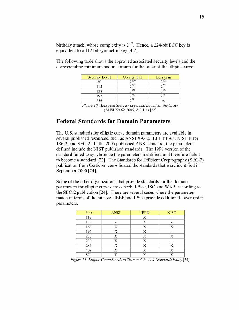
birthday attack, whose complexity is 2n/2. Hence, a 224-bit ECC key is equivalent to a 112 bit symmetric key [4,7]. The following table shows the approved associated security levels and the corresponding minimum and maximum for the order of the elliptic curve.
Security Level Greater than Less than
80 2160 2223 112 2223 2255 128 2255 2383 192 2383 2511 256 2511 ∞
Figure 10: Approved Security Level and Bound for the Order (ANSI X9.62-2005, A.3.1.4) [22]
Federal Standards for Domain Parameters The U.S. standards for elliptic curve domain parameters are available in several published resources, such as ANSI X9.62, IEEE P1363, NIST FIPS 186-2, and SEC-2. In the 2005 published ANSI standard, the parameters defined include the NIST published standards. The 1998 version of the standard failed to synchronize the parameters identified, and therefore failed to become a standard [22]. The Standards for Efficient Cryptography (SEC-2) publication from Certicom consolidated the standards that were identified in September 2000 [24]. Some of the other organizations that provide standards for the domain parameters for elliptic curves are echeck, IPSec, ISO and WAP, according to the SEC-2 publication [24]. There are several cases where the parameters match in terms of the bit size. IEEE and IPSec provide additional lower order parameters.
Size ANSI IEEE NIST 113 - X - 131 - X - 163 X X X 193 X X - 233 X X X 239 X X - 283 X X X 409 X X X 571 X X X
Figure 11: Elliptic Curve Standard Sizes and the U.S. Standards Entity [24]

20
In the United States, ANSI is used as an organization for retaining and distributing standards that originate from other entities, so as to confirm that the standards used are those associated with doing business with the United States. Where as IEEE and NIST are organizations that create and publish national standards. For more detail on the associated domain parameters in binary Galois fields, Appendix 2 has the full set of the NIST parameters [35]. For binary Galois fields, within a polynomial basis, the approved reduction polynomials are provided in the table below. These particular polynomials were chosen because they are ideally suited for use in fast-reduction algorithms, which are used to accelerate the mathematics associated with ECC [1, 22].
Field Reduction Polynomial F2113 f(x) = x113 + x9 + 1
F2131 f(x) = x131 + x8 + x3 + x2 + 1 F2163 f(x) = x163 + x7 + x6 + x3 + 1 F2193 f(x) = x193 + x15 + 1 F2233 f(x) = x233 + x74 + 1 F2239 f(x) = x239 + x36 + 1 F2283 f(x) = x283 + x12 + x7 + x5 + 1 F2409 f(x) = x409 + x87 + 1 F2571 f(x) = x571 + x10 + x5 + x2 + 1
Figure 12: Reduction Polynomials in Binary Galois Fields [22]
International Standards NIST and IEEE are not the only organizations that have defined elliptic curve standards. In the international community, organizations such as ISO/IEC, have determined standards in conjunction with NIST, IEEE, and ANSI. These organizations are a part of the Standards for Efficient Cryptography Group, SECG. This group works on operability and compatibility issues between all of the standards. [1]

21
Chapter 4 Domain Parameter Generation & Validation
• Algorithms for Generating Domain Parameters o Generating a Verifiably Random Elliptic Curve o Basis Conversion o Determining the Order, n o Primality Testing Algorithms o Point Counting Algorithms o Generating a Verifiably Random Base Point
• Validation of Domain Parameters

22
Algorithm for Generating Parameters There are a few stages in the generation process for randomly verifiable domain parameters. They can be calculated pseudo-randomly, as is described below, or they can be selected from the NIST and IEEE standards, looked up in the ANSI X9.62 document, or the SEC-2 document [22, 24, 26].
Figure 13: Ways to Obtain the Domain Parameters
The parameters, as mentioned in the previous chapter are the following:
1. m = field size and power or the leading x of the irreducible polynomial
2. f(x) = irreducible polynomial modulus for polynomial basis 3. a = coefficient for the elliptic curve equation 4. b = coefficient for the elliptic curve equation 5. P = (xp, yp), a point on the elliptic curve 6. n = the order of the point, P 7. h = the cofactor, such that h = #E(F (2m) )/ n
h ∈ { 2, 4 } 8. s = seed for the hash function for random parameter generation
Since obtaining the domain parameters from approved, published standards is quite simplistic, the generation of verifiably random parameters will be examined in this chapter. The following figure shows that steps involved in generating the necessary domain parameters.
Generating Verifiably
Random Domain Parameters
Obtain Domain Parameters for
ECC
Obtain Domain Parameters from
Standards Documents

23
Figure 14: Steps in Obtaining the Domain Parameters[22] Verifiably Random Domain Parameters The first step in the generation of domain parameters is the generating of the appropriate elliptic curve. An elliptic curve in binary Galois fields requires values for a and b, and that b does not equal 0. This is done with the use of a seed value, an approved hash function with an output of length t, and identifying field size for this set of parameters. The field size is related to the chosen security level. At a minimum, the field size should be ≥ 2163, where 163 denotes the smallest NIST standard value. The following is a listing of the steps in obtaining the Elliptic Curve. It is compiled from ANSI X9.62-2005[1, 22].
Generating a Verifiably Random Elliptic Curve
Determining the Order of the Elliptic Curve
Generating a Base Point on the Elliptic Curve
Primality Testing Algorithm
Secure Hash Algorithm
Point Counting Algorithms
Domain Parameters
Secure Hash Algorithm
Half-Trace Algorithm

24
Figure 15: Algorithm for Generating Verifiably Random Elliptic Curves[22]
The criteria for elliptic curve generation are that m is a prime, and that the security of the hash function must be equal to or greater than the overall security level desired by the user. The value of m is very small, and confirming m is a prime is trivial. The hash functions that are available, currently, are SHA-1, SHA-256, SHA-384, and SHA-512 [34]. Until the SHS changes, these are the available algorithms to be implemented, and currently are implemented in Certicom’s software package which implements ECC for the federal standards [20, 21, 40]. Determining the Order for the Elliptic Curve Determining the order, n, for an elliptic curve requires a means by which to count the number of points associated with the curve. Koblitz curves also utilize a cofactor term, whose value is either 2 or 4. This is essential so as to be able to compute the base point of the associated elliptic curve. By Hasse’s theorem[6], the number of points follows the following equation:
1. Let
!
m = log2 q" #
2. Let
!
s =(m "1)
t
#
$ # %
& %
3. Let
!
k = m " s # t if q is even, and for binary Galois fields, it is. 4. Compute H = HASH (Seed) where the hash function is approved as
a Secure Hash Standard (SHS) 5. Convert H to an integer e, using data conversion techniques.
• This is a conversion from a hexadecimal value to an integer 6. Let
!
c0
= emod2k
7. For j from 1 to s, let
!
c j = HASH((Seed + j)mod2g , where g is bit-
length of the binary representation of Seed + j. 8. Let
!
c = c0" 2
ts+ c
1" 2
t(s#1)...+ c
s
9. Convert c to a field element r • This is done by taking the hex-value of c and converting to
a bit string of length m. 10. Choose an element a of the field F (2m). For all of the NIST
approved parameters, this value, a = 1. 11. Lastly, since q is even, set b = r. If b = 0, then “failure.”

25
!
2m
+1" 2m ≤ #E (F(2m))≤
!
2m
+1+ 2m
In order to compute the value accurately, efficient point counting algorithms need to be implemented. A criterion for the order is that the order is a prime number. This is confirmed with an efficient primality-testing algorithm. The types of primality testing available and used in the standards will be discussed shortly.
Point-Counting and Calculating Order The simplest method for computing the order of an elliptic curve is by implementation of an algorithm based on a Lucas Sequence [8]. A Lucas Sequence solves for a value based on previously computed values, similarly as a recursion. Just as in a recursion there is a base case, point counting in binary Galois fields has a base case for the computation. Theorem 4.12 [6] computes the number of points on an elliptic curve for F(qm) given that F(q) can be solved easily. For binary Galois fields, q = 2, and the first portion of the theorem is utilized to compute the base value for µ. For the number of points on the elliptic curve on F(q), where q is prime, the points that satisfy the elliptic curve equation with the modulus of the field. The points on
E : y2 + xy = x3+ ax2 + 1
in F(2) are as follows for the condition that a = 0, or a = 1.
E(F(2)) = { (∞, ∞), (0, 0), (0 , 1), (1, 0), (1, 1) }
THEOREM 4.12 Let #E(F(q)) = q + 1 – µ. Write X2 – aX + q = (X - α)(X - β). Then
#E(F(qn)) = qn + 1 – (αn + βn) for all n ≥ 1.

26
The maximum number of points is five, and the subset always has (∞, ∞) as one of the allowable points. For binary Galois fields, elliptic curve equations are of the form:
y2 + xy = x3 + ax2 + b For NIST approved curves, a = 1 and b is a randomly verifiable integer, not equal to zero, or a predefined value from the federal standards. For Koblitz curves, the elliptic curve has b = 1, and a is an element of {0, 1}. In order to solve (αn + βn), from Theorem 4.12, an associated lemma is implemented which utilizes the Lucas sequence. Rearranging the base equation from theorem 4.12:
µ =q + 1 – #E(F(q)) = s1
Utilizing lemma 4.13 and theorem 4.12 computes the number of points on the elliptic curves of higher degree.
LEMMA 4.13 Let sn = (αn + βn). Then s0 = 2, s1 = µ, and sn+1 = µsn - qsn-1 for all n ≥ 1.
Example: E: y2 + xy = x3 + 1x2 + b for F(2163)
If b mod 2 = 1, then E(F(q)) = { (∞, ∞), (0 , 1) }. This is used to solve for µ.
µ =2 + 1 – 2 = 1 = s1
If b mod 2 = 0, then E(F(q)) = { (∞, ∞), (0, 0), (1, 0), (1, 1) } In this case:
µ =2 + 1 – 4 = -1 = s1
Therefore, if µ = 1, then s0 = 2, s1 = 1, and sn+1 = sn - 2sn-1. s2 = s1 - 2s0 = (-1) – 2( 2) = -3 s3 = s2 - 2s1 = (-3) – 2(-1) = -5 s4 = s3 - 2s2 = (-5) – 2(-3) = 1 … s163 = s162 - 2s161 = - 4845466632539410776804317
#E(F(2163)) = 2163 + 1 – s163

27
There are other methods for point counting in Galois fields. The Schoof algorithm, established in 1985, is a slow, polynomial time algorithm. Others have developed much quicker algorithms for general fields. These other algorithms are:
Schoof, Elkies, Atkins Algorithm [7, 28, 36] AGM – Arithmetic Geometric Mean [1, 32] SST – Satoh, Skjernaa, Taguchi algorithm [1, 29, 32] MSST – Modified Satoh, Skjernaa, Taguchi algorithm [32]
These algorithms would certainly provide the necessary results for point counting, however for binary Galois fields, these provide much more computational capability than is necessary.
Primality Testing Algorithms There are several algorithms that have been developed for computing the primality of a number, some more efficient than others. The one utilized by the federal standards is the Miller-Rabin primality test [22], which was developed in 1985. This is also known as a “Strong Pseudoprimality Test” [7]. This algorithm has a O (log n)3 runtime, which considerably better than the others. However, it does erroneously identify a number as a prime with a
Example (continued): 11692013098647223345629478661730264157247460343808
+ 1 - (- 4845466632539410776804317)
11692013098647223345629483507196896696658237148126
The order is a large value that is prime. Obviously, since this number is even, it is not prime. Dividing this result by 2 confirms that 2 is the cofactor and the order is a prime whose value is:
order = 5846006549323611672814741753598448348329118574063

28
small degree of error, given by the equation below, where k is the number of randomly selected bases.
!
P(error) = 14k
This error probability is better than the Euler’s Pseudoprimaility Test, by a factor of 2k. Other algorithms are utilized to reduce this error probability, but do so in an inefficient manner. The Goldwasser-Kilian Algorithm was developed in 1988, however its’ runtime is O (log n)10+c , where c is a constant. This algorithm also attempts to implement the Schoof Point Counting Algorithm [7]. In Atkin and Morain’s 1993, publication “Elliptic Curves and Primality Proving,” they developed a new algorithm which avoids the problems of the Goldwasser-Kilian algorithm. It is simply referred to as ECPP, Elliptic Curves Primality Proving. Its’ runtime is O (log n)6+ε. It is the combination of the Miller-Rabin algorithm and the ECPP algorithm that constitute the Practical Primality Test [7]. ECPP is a zero-error probabilistic test, which can be utilized to verify the Miller-Rabin test. The Miller-Rabin and the ECPP tests have different runtimes. The Practical Primality Test implements both of these methods as means to validate the value. If a number under test passes both of these conditions, it is confirmed to be a prime number. Since the Miller-Rabin can confirm a number is composite, a prime value may not necessarily be a prime. Therefore, ECPP can be utilized to verify primality, and only be used for questionable cases since its runtime is larger than that of Miller-Rabin. Generating the Base Point The base point is a point on the designated elliptic curve. For verifiably random elliptic curves, a seed value is used, and the standard algorithm provided by ANSI is used for creating the base point. Otherwise, one can use the values provided in the NIST and IEEE standards. The following is a step-by-step description of the algorithm for which a seed is used from the ANSI X9.62-2005 standard [22]. The necessary input parameters are E=(F(2m), a, b), the cofactor h, a prime n, and a bit string Seed.

29
Figure 16: Base Point Generation (ANSI X9.62-2005)[22] By computing the base point, the final values, which are characterized as the domain parameters have been calculated. These values now can be utilized for elliptic curve cryptography, digital signatures, and authentication. Validating Domain Parameters The validation of the elliptic curve domain parameters can be simplified into two categories; validating an Elliptic Curve, and validating a Base Point. The validation of the elliptic curve has four criteria for binary Galois fields [22].
• The field must be of the form F(2m), where m = prime. • The coefficients of the curve, a and b, when converted to binary must
have a bit-length of m bits.
1. Set base = 1 2. Set element = 1 3. Convert base and element to octet strings Base and Element,
respectively 4. Compute H = HASH (“Base Point” || Base || Element || Seed)
where the hash function is approved as a Secure Hash Standard (SHS)
5. Convert H to an integer e, using data conversion techniques.
6. If
!
e
2q
"
# "
$
% $ =
2hashlen
2q
"
# "
$
% $ then increment element and go back to step 3.
7. Let
!
t = emod2q; such that
!
{t " N |
!
0 " t " 2q #1}
8. Let
!
x = tmodq and
!
z =t
q
"
# " $
% $
9. Choose an element x of the field F(2m). 10. Recover the field element, y, using point compression over binary
fields from (x, z). The point compression algorithm utilizes functions for calculating the quadratic of a binary Galois field, and a Half-Trace function for polynomial basis calculations.
11. With x and y, the point P has been calculated.

30
• The value of b ≠ 0. • The seed used to generate the curve must match the seed provided.
Validation of a base point has some additional constraints [22].
• The base point, P, is not the infinity point. • G = hP, where P = (xP , yP), and h is the cofactor. • P = (xP , yP), and each component has bit-length equal to m. • (xP , yP) must satisfy the associated elliptic curve equation. • nP = ∞. • If G is not a valid base point then increment base and go back to Step
2 in the base-point generation algorithm, unless base > 10h2, in which case, output "Failure".
• If P is generated randomly, utilize the parameters (h, n, seed) to recreate the base point, and compare with the value received. These values should match.
• Verify that the MOV and Anomalous conditions are met. In the current version of the ANSI standard, X9.62-2005, the generation and validity of the domain parameters is provided in Annex A.3.5.2 and A.3.5.3.

31
Chapter 5 Selection Criteria for Parameter Generations
• Pseudo-Random Number Generation • Selection of Security Level, and m
o Koblitz Curve • Curve Coefficients • Cofactors
• 32-Bit Architecture • Selection of Basis
o Polynomial Basis & Fast Reduction algorithm o Normal Basis
• Selection of Hash Algorithm (SHA-1 to SHA-512) • Criteria for Elliptic Curve Security
o MOV Criteria o Anomalous Condition
32
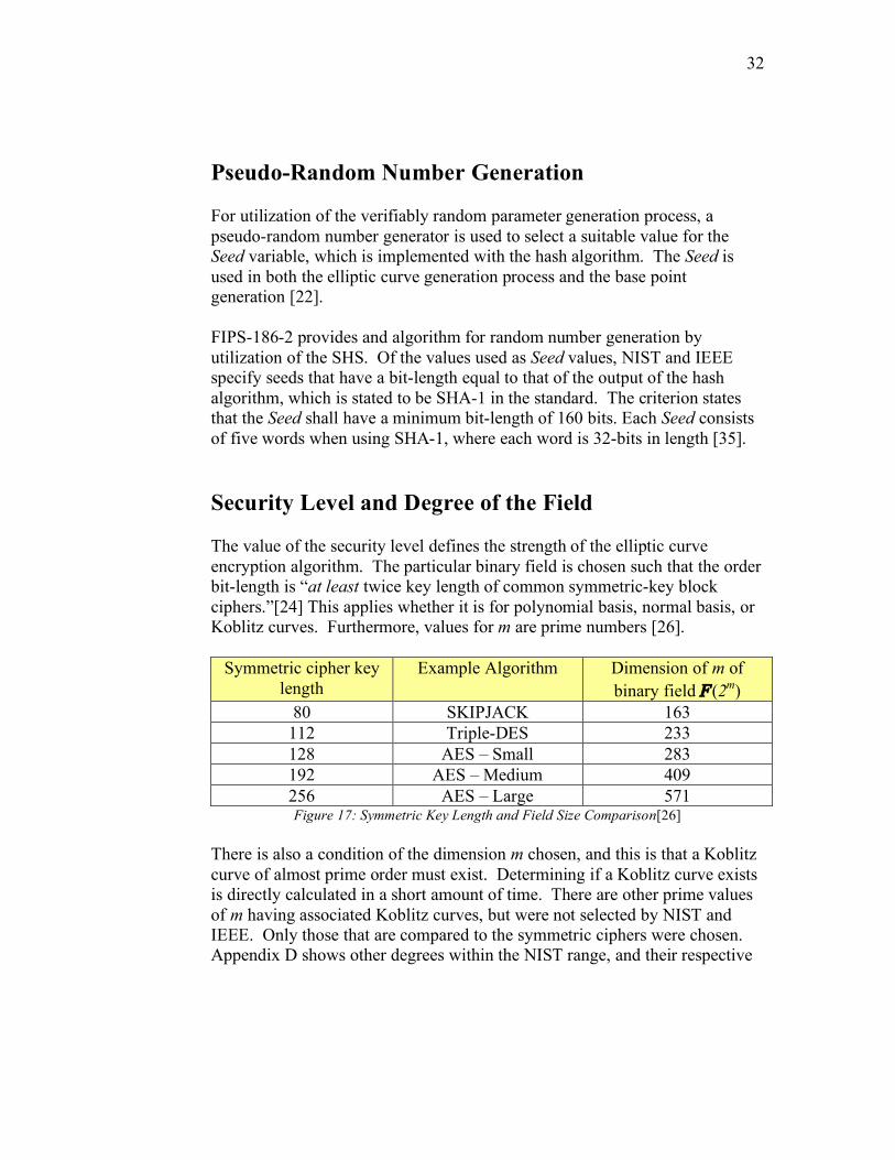
Pseudo-Random Number Generation For utilization of the verifiably random parameter generation process, a pseudo-random number generator is used to select a suitable value for the Seed variable, which is implemented with the hash algorithm. The Seed is used in both the elliptic curve generation process and the base point generation [22]. FIPS-186-2 provides and algorithm for random number generation by utilization of the SHS. Of the values used as Seed values, NIST and IEEE specify seeds that have a bit-length equal to that of the output of the hash algorithm, which is stated to be SHA-1 in the standard. The criterion states that the Seed shall have a minimum bit-length of 160 bits. Each Seed consists of five words when using SHA-1, where each word is 32-bits in length [35]. Security Level and Degree of the Field The value of the security level defines the strength of the elliptic curve encryption algorithm. The particular binary field is chosen such that the order bit-length is “at least twice key length of common symmetric-key block ciphers.”[24] This applies whether it is for polynomial basis, normal basis, or Koblitz curves. Furthermore, values for m are prime numbers [26].
Symmetric cipher key length
Example Algorithm Dimension of m of binary field F(2m)
80 SKIPJACK 163 112 Triple-DES 233 128 AES – Small 283 192 AES – Medium 409 256 AES – Large 571 Figure 17: Symmetric Key Length and Field Size Comparison[26]
There is also a condition of the dimension m chosen, and this is that a Koblitz curve of almost prime order must exist. Determining if a Koblitz curve exists is directly calculated in a short amount of time. There are other prime values of m having associated Koblitz curves, but were not selected by NIST and IEEE. Only those that are compared to the symmetric ciphers were chosen. Appendix D shows other degrees within the NIST range, and their respective

33
Koblitz curve orders with their cofactors. Additional values for m beyond the 571 field were also calculated. Therefore, the next choice of polynomial basis Galois field would be 701. This would provide a larger value for m with more security. The figure below shows a comparison for the key size that is necessary to yield that same level of security. A 160-bit ECC key is comparable to a 1024-bit RSA key.
Figure 18: ECC to RSA Key Length Comparison[4] A 701-bit ECC key would exceed the current security standards, yet still be able to utilize the fast reduction algorithms available for the standards. The associated irreducible polynomial is as follows.
f(x) = x701 + x16 + x4 + x2 + 1 Fast reduction algorithms have been defined for the five federal standards and have an upper limit of 1140. They allow compatibility with the standards even if non-standard fields are chosen.
32-bit Architecture The entire implementation of generating elliptic curve parameters utilizes 32-bit architecture. It is exemplified in all aspects of the process. It is utilized for the hash algorithm, modular reduction, and polynomial multiplication [22]. Many new computers are manufactured with 64-bit architecture, such as the Apple MacBook. Currently, not many resources would benefit from higher
RSA/DSA (modulus size in bits)
512
1024
2048
3072
7680
15360
ECC- Based Scheme (size of n in bits)
112
160
224
256
384
521

34
bit architecture in regards to needed memory allocation, mapping, and reverse compatibility issues. Therefore, unless a specific application requires higher bit architecture, the current implementations are quite sufficient. The only exception is the pending elimination of the SHA-1 hash algorithm. SHA-256, SHA-384, and SHA-512 are very beneficial, and will provide the needed hashing of data for a long time, until SHA-3 is chosen to replace existing hash functions as a new standard in 2012 [19, 20]. Selection of Basis The selection of the basis to use for generation of parameters is not tremendously critical, between polynomial and normal bases. These two bases can be used interchangeably by means of a conversion algorithm. NIST and IEEE specify the necessary conversion value that is used to create an m-by-m conversion matrix. Unique standard sets of values are provided to convert from a normal basis to polynomial, and vice versa. The most ideal choice for implementations is the Koblitz curves, due their efficiency [22, 35].
Fast reduction For polynomial basis computations, mathematical computations are performed with the modulus of the irreducible polynomial. However, even with selection of a different field size, the mathematic functions can be “reduced” so as to use the modulus associated with the five NIST standards [1].
Binary polynomial size <325 <465 <565 <817 <1140 NIST Field 163 233 283 409 571
Based on the available fast reduction algorithms, no field size greater than 1140 can be used. However, reduction can be calculated for fields of size 2m-2 by a modular reduction algorithm which calculates the reduction on a bit-by-bit level [1]. The available fast reduction algorithms are implemented on word lengths of 32-bits. A 64-bit implementation would not double the efficiency of the elliptic curve algorithms. Memory overhead and lack of compatibility with 32-bit systems are a drawback to current usage. Associated loops in the reduction algorithms would be halved, but the bitwise operations would increase, if one were to repeat the procedure for the existing standard fields. With 64-bit architecture, larger field sizes may be considered, and weighing the considerations of

35
security and computing time would be essential. 64-bit instructions, with the increased length have a decrease in decoding rate [30]. Selection of Hash Algorithm The choice of the hash algorithm to be implemented for the generation of domain parameters is dependent on the security level desired by the user. The federal standards identify SHA-1 as the hash used for the generation of the standard domain parameters. However, with the eventual elimination of SHA-1, it would be beneficial to implement other, more stable hash functions in the interim. It would also be beneficial to choose a field size comparable in security level to that of the hash function.
Field Size SHA-1 SHA-256 SHA-384 SHA-512 Hash Output Size 160 256 384 512
Field Size 163, 233 283 409 571 Figure 19: Utilization of Other Existing Hash Functions
This recommendation would be applicable until 2012 when a new hash standard will be determined, SHA-3. Note that only the hashs defined by FIPS 180-2 are identified. SHA-224 is identified in the FIPS 180-3 publication which is still in draft form, and is not identified here until this its official release. Security Criteria
MOV Attack The MOV attack is named so after Menezes, Okamoto, and Vanstone. It is an attack on an elliptic curve by a reduction of the discrete log problem to the finite field, F(qB). Hence for binary Galois fields, F(2B). The coefficient, B, is the MOV threshold. Selection of a relatively large value for the threshold must prove to results in a difficult discrete logarithmic problem over F(2). The MOV threshold in the federal standards dictates that B ≥ 100 [22, 35]. Since NIST provides standards whose degrees of their respective fields are at least 163, the MOV criterion is satisfied. Hence, degrees smaller than 100 can not be chosen as viable choices for the purposes of secure parameter generation and validation.

36
Anomalous Condition Elliptic curve discrete logarithm problem in anomalous curves have been shown to be easily solved. The anomalous condition is achieved when the number of points on an elliptic curve, in a designated field does not equal the size of the binary field.
#E(F(2m))≠ 2m Most elliptic curves over a field F(2m) will indeed satisfy the Anomalous condition, making them resistant to anomalous attack [22, 35].

37
Chapter 6 Algorithms and Analysis
• Generating and Validating a Randomly Verifiable Elliptic Curve o Implementation of the Algorithm
• Point Counting o “Lucas Sequence”
• Criteria of the Sub-sections of the Algorithms o Hash Functions & Output o 32-Bit Word Lengths o Point-Counting Algorithm o Fast Reduction with an Irreducible Polynomial Modulus

38
Algorithms In understanding the associated procedures and constraints with generating randomly verifiable parameters, certain algorithms from the ANSI standard were utilized. Implementation of the algorithms was done in Java, and in some cases utilizing existing code, such as the Schoof algorithm [7, 14]. Generating Elliptic Curve Implementation of the randomly verifiable elliptic curve generator from ANSI [22] proved to be quite challenging mainly due to the multiple data conversions necessary. The associated code was a modification to a compilation of some readily available applications. The Java code implementing the SHA-1 hash came from www. anyexample.com [15]. This code provided the baseline on which to build the generator program. In implementation of the generation algorithm, it became apparent that utilizing other hash functions is done simply by substituting the existing specified hash for another hash function of choice. SHA-256, SHA-384, and SHA-512 can be specified directly, and they adhere to the SHS [15]. As a means to confirm the program was functioning properly, and would generate the appropriate results, the NIST approved value for the Seed for the 163-bit ECC domain parameters was used. The output that resulted was the NIST specified value for the b coefficient, in Normal Basis. Conversion to a polynomial basis requires the creation of the conversion matrix, as well as the calculations of the associated roots, in the proper basis. This procedure includes the roots of the irreducible polynomial equation. For the standards that exist, the creation of the conversion matrix is simplified by multiplying and reducing the critical rows of data to make the matrix. This particular conversion matrix is a 163-by-163 bit array. The following is an example in F(24) [26].

39
!
n = 1 0 1 0[ ]
" =
1 1 0 0
1 1 1 1
1 0 1 0
1 0 0 0
#
$
% % % %
&
'
( ( ( (
n ) " = 0 1 1 0[ ]mod(2)
Using this simple example enforces the understanding that a larger scale conversion, such as that for the NIST 163-bit value for b. will yield [35]: b = 6645f3cacf1638e139c6cd13ef61734fbc9e3d9fb (Normal) b = 20a601907b8c953ca1481eb10512f78744a3205fd (Polynomial) With the confirmation that the value for b was computed correctly, a randomly generated seed was calculated using Matlab. The function is shown below.
In addition to the random seed, a different field size was chosen, one whose Koblitz curve exists, but is not one of the standard five dataset. The degree of the field chosen was 311. The results of the curve generation are provided in the following chapter. Computing the Order Similarly, as with the curve generator, a known test case was first used to confirm the functionality and correctness of the Schoof program, which was available from www.shamus.ie [14]. The consideration with using the
function prng n = 16; f = dec2hex(ceil(n.*rand(40,1))-1); out = f(1:40)'

40
“schoof2.exe” program is that the input is in polynomial basis [14]. This was confirmed by testing the NIST data as input. This implementation of the Schoof algorithm took several minutes for the 163-bit input. Larger input takes on the order of hours to days to complete. The long calculation time lead to examining another algorithm, one based on a Lucas sequence [6, 8]. This worked very well in computing the elliptic curve order in a matter of seconds. Its only input was the size of the field, m. The condition associated with this algorithm, is that it only applies for small prime numbers, q, for F(qm). In the case of binary Galois fields, q = 2. The algorithm computes the order for the base point of the Koblitz curves. This was confirmed by testing various input values, and comparing the result with known result in [1]. The benefit of this algorithm is that it can confirm orders quickly for Koblitz curves, and in so doing, it provides other field sizes for non-Koblitz binary Galois elliptic curves. This also becomes an advantage if Koblitz curves are actually needed in regards to a hardware implementation. Appendix D shows the results of computing the order beyond a 571-bit field size.

41
Chapter 7 Results and Conclusion
• Results of Implementation of Algorithms • Results of Case Study • Closing Summary • Future Work
42
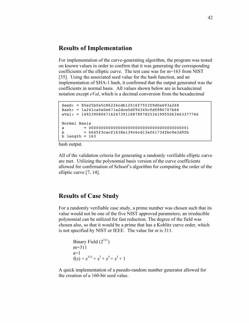
Results of Implementation For implementation of the curve-generating algorithm, the program was tested on known values in order to confirm that it was generating the corresponding coefficients of the elliptic curve. The test case was for m=163 from NIST [35]. Using the associated seed value for the hash function, and an implementation of SHA-1 hash, it confirmed that the output generated was the coefficients in normal basis. All values shown below are in hexadecimal notation except eVal, which is a decimal conversion from the hexadecimal
hash output. All of the validation criteria for generating a randomly verifiable elliptic curve are met. Utilizing the polynomial basis version of the curve coefficients allowed for confirmation of Schoof’s algorithm for computing the order of the elliptic curve [7, 14]. Results of Case Study For a randomly verifiable case study, a prime number was chosen such that its value would not be one of the five NIST approved parameters; an irreducible polynomial can be utilized for fast reduction. The degree of the field was chosen also, so that it would be a prime that has a Koblitz curve order, which is not specified by NIST or IEEE. The value for m is 311.
Binary Field (2311) m=311 a=1 f(z) = z311 + z7 + z5 + z3 + 1
A quick implementation of a pseudo-random number generator allowed for the creation of a 160-bit seed value.
Seed: = 85e25bfe5c86226cdb12016f7553f9d0e693a268 Hash: = 1a241ca0a0e671a2dce5df94340cfdf886707b66 eVal: = 149239080671624739118878978253419955063463377766 Normal Basis a = 00000000000000000000000000000000000000001 b = 6645f3cacf1638e139c6cd13ef61734fbc9e3d9fb b length = 163

43
s = 0x FA7D88A5 39D62746 D6652416 44617B3C 16030324
Taking the randomly generated seed and using it as the input for the elliptic curve generator, setting m = 311, and using the SHA-1 hash algorithm, results in the following value for the b-coefficient. The a-coefficient was set to 1, so as to be identical to the NIST format.
b = 0x 004087c3 91766f31 86287017 ed2aa5a0 743d6c8e a5408fd0 e4685d67 48182e94 09c07c76 cf66484c
The result of the SHA-1 hash and the integer value of the hash output are shown below.
Once again, the criteria for valid elliptic curve generation are met. The coefficients have bit-length equal to m, which is a prime number, and neither coefficient is 0. The seed, which generated the coefficients, is provided allowing for verification of the parameters. Determining higher order fields were also computed for cases where a Koblitz curve of the form y2 + xy = x3+ x2 + 1 exists. Prime numbers were chosen above the maximum NIST value of 571. The first three primes that met this criterion were 701, 1153, and 1249. The bit-length for the order of these fields is growing comparable to RSA, and exceeds the 1024 minimum RSA requirement. The standard reduction algorithms have an upper limit of 1140 bits, however higher order fields can be used with the implementation of a bit-by-bit reduction algorithm. These orders are shown in Appendix D.
Seed: = FA7D88A539D62746D665241644617B3C16030324 Hash: = a2c087c391766f3186287017ed2aa5a0743d6c8e eVal: = 929150074658595225474527593156946520741668285582 Normal Basis a = 000000000000000000000000000000000000000000000000000000000000000000000000000001 b = 4087c391766f3186287017ed2aa5a0743d6c8ea5408fd0e4685d6748182e9409c07c76cf66484c b length = 311

44
Summary Implementation of the algorithms must be done with extreme attention and focus on the basis that one is working with, as well as conversions. Since the SHS and ECC parameters are based on 32-bit word lengths, this is ideal for the older computer processors and future processors. This allows for ECC algorithms to be backwards compatible with previous versions. The 64-bit processors are gradually becoming more common, as will the software. This includes the encryption packages that need to be written for this architecture. In regards to the NIST standards for parameters, for immediate implementation with key-pair generation, the readily available parameters are ideal. Creation of custom parameters requires a through understanding of the application and whether it is to be implemented in software or hardware. For hardware implementations, Koblitz curves are ideal.
Criteria Synopsis
• Pseudo-Random Seed for hash functions of bit-length equal to the degree of the field, even though the hash functions pad the seed.
• For NIST requirement, a = 1, and b ≠ 0 having bit-length equal to the degree of the field. For Koblitz curves, b = {0, 1}
• Hash algorithm must have a security level greater than or equal to the security level of the elliptic curve field degree, with the understanding that the SHA-1 hash function should be eliminated as a standard, and replaced with the SHA-256 function defined in FIPS 180-2 until the new SHS is determined and released publically.
• Computing the necessary orders should be performed using the most efficient algorithms available, such as SST, AGM, or MSST. However, the method used for Koblitz curves is beneficial to select other field degrees.
• Conversion algorithms and fast reduction algorithms should be readily computable for any field size, not just specific to the standards.

45
Future Work Further research would consist of implementation of the most recent algorithms, such as the MSST algorithm so as to compute the order very quickly for general fields. As the newest standard hash algorithm becomes published, implementation of the hash with the elliptic curve parameter generating algorithms, and testing will be essential for compatibility with the elliptic curve domain parameter generation procedures. In order for simplified user access to the generation of parameters, a robust GUI could be developed so as to select the criteria for the elliptic curve parameters. Everything from security level, hash algorithm, standard NIST parameters or randomly verifiable ones should be readily selectable for the end-user. This can also be utilized as a learning tool. Algorithms associated with fast reduction and modular reduction should also be implemented. With an entire set of algorithms and features, an application package could be developed for commercial use on multiple platforms. It would also be of interest to implement algorithms that do not reduce field elements to the five NIST standards, but rather are completely generic based on field selection, only. Lastly, a recommendation should be made to NIST and IEEE, that the 163 and 233 bit domain parameters either use a stronger hash function as standard, or be eliminated from the federal standards.

46
Appendices Appendix A – Abbreviations ANSI American National Standards Institute DSA Digital Signature Algorithm DSS Digital Signature Scheme ECC Elliptic Curve Cryptography/Cryptosystem ECPP Elliptic Curve Primality Proving GF Galois Field, also denoted F GNB Gaussian Normal Basis IEEE Institute of Electrical and Electronics Engineers MSST Modified Satoh-Skjernaa-Taguchi point counting algorithm NIST National Institute of Standards and Technology PPB Pentanomial Polynomial Basis RSA Rivest, Shamir, Adleman SEA Schoof-Elkies-Atkin point counting algorithm SHA Secure Hash Algorithm SHS Secure Hash Standard SST Satoh-Skjernaa-Taguchi point counting algorithm TPB Trinomial Polynomial Basis

47
Appendix B – NIST Standards The following values are the NIST recommended standard parameters for elliptic curves over binary fields in a polynomial basis and normal basis. The NIST standards are for bit lengths of 163, 233, 283, 409, and 571. These same bit lengths are utilized by Kolbitz Elliptic Curves, for which the parameters are uniquely specific. The conversion algorithm for converting from a polynomial to a normal basis, or vice versa, is provided in FIPS 186-2 as well as other standards [22, 26, 35]. m the extension degree of the binary field (GF(2m))
a,b the coefficients of the elliptic curve equation: y2 + xy = x3 + ax2 + b
f(z) the irreducible polynomial of degree m s seed value for randomly generating the coefficients of
the elliptic curve r base point order h the cofactor xG, yG the (x, y) value for the base point, G
Binary Field (2163) m=163 a=1 h=2 f(z) = z163 + z7 + z6 + z3 + 1 s = 0x 85e25bfe 5c86226c db12016f 7553f9d0 e693a268 r = 5846006549323611672814742442876390689256843201587
Polynomial Basis: b = 0x 2 0a601907 b8c953ca 1481eb10 512f7874 4a3205fd xG = 0x 3 f0eba162 86a2d57e a0991168 d4994637 e8343e36 yG = 0x d51fbc6c 71a0094f a2cdd545 b11c5c0c 797324f1
Normal Basis: b = 0x 6 645f3cac f1638e13 9c6cd13e f61734fb c9e3d9fb xG = 0x 311103c1 7167564a ce77ccb0 9c681f88 6ba54ee8 yG = 0x 3 33ac13c6 447f2e67 613bf700 9daf98c8 7bb50c7f
Binary Field (2233) m=233 a=1

48
h=2 f(z) = z233 + z74 + 1 s = 0x 74d59ff0 7f6b413d 0ea14b34 4b20a2db 049b50c3 r = 690174634679056378743475586227702555583981273734\
5013555379383634485463 Polynomial Basis:
b = 0x 00000066 647ede6c 332c7f8c 0923bb58 213b333b 20e9ce42 81fe115f 7d8f90ad
xG = 0x 000000fa c9dfcbac 8313bb21 39f1bb75 5fef65bc 391f8b36 f8f8eb73 71fd558b
yG = 0x 00000100 6a08a419 03350678 e58528be bf8a0bef f867a7ca 36716f7e 01f81052
Normal Basis:
b = 0x 000001a0 03e0962d 4f9a8e40 7c904a95 38163adb 82521260 0c7752ad 52233279
xG = 0x 0000018b 863524b3 cdfefb94 f2784e0b 116faac5 4404bc91 62a363ba b84a14c5
yG = 0x 00000049 25df77bd 8b8ff1a5 ff519417 822bfedf 2bbd7526 44292c98 c7af6e02
Binary Field (2283) m=283 a=1 h=2 f(z) = z283 + z12 + z7 + z5 + 1 s = 0x 77e2b073 70eb0f83 2a6dd5b6 2dfc88cd 06bb84be r = 7770675568902916283677847627294075626569625924376\
904889109196526770044277787378692871 Polynomial Basis:
b = 0x 027b680a c8b8596d a5a4af8a 19a0303f ca97fd76 45309fa2 a581485a f6263e31 3b79a2f5
xG = 0x 05f93925 8db7dd90 e1934f8c 70b0dfec 2eed25b8 557eac9c 80e2e198 f8cdbecd 86b12053
yG = 0x 03676854 fe24141c b98fe6d4 b20d02b4 516ff702 350eddb0 826779c8 13f0df45 be8112f4
Normal Basis:
b = 0x 0157261b 894739fb 5a13503f 55f0b3f1 0c560116 66331022 01138cc1 80c0206b dafbc951
xG = 0x 0749468e 464ee468 634b21f7 f61cb700 701817e6 bc36a236 4cb8906e 940948ea a463c35d
yG = 0x 062968bd 3b489ac5 c9b859da 68475c31 5bafcdc4 ccd0dc90 5b70f624 46f49c05 2f49c08c

49
Binary Field (2409) m=409 a=1 h=2 f(z) = z409 + z87 + 1 s = 0x 4099b5a4 57f9d69f 79213d09 4c4bcd4d 4262210b r = 66105596879024859895191530803277103982840468\
96428121928464879830415777482737480520814372\ 362179110965979867288366567526771
Polynomial Basis:
b = 0x 0021a5c2 c8ee9feb 5c4b9a75 3b7b476b 7fd6422e f1f3dd67 4761fa99 d6ac27c8 a9a197b2 72822f6c d57a55aa 4f50ae31 7b13545f
xG = 0x 015d4860 d088ddb3 496b0c60 64756260 441cde4a f1771d4d b01ffe5b 34e59703 dc255a86 8a118051 5603aeab 60794e54 bb7996a7
yG = 0x 0061b1cf ab6be5f3 2bbfa783 24ed106a 7636b9c5 a7bd198d 0158aa4f 5488d08f 38514f1f df4b4f40 d2181b36 81c364ba 0273c706
Normal Basis:
b = 0x 0024d065 1c3d3772 f7f5a1fe 6e715559 e2129bdf a04d52f7 b6ac7c53 2cf0ed06 f610072d 88ad2fdc c50c6fde 72843670 f8b3742a
xG = 0x 00ceacbc 9f475767 d8e69f3b 5dfab398 13685262 bcacf22b 84c7b6dd 981899e7 318c96f0 761f77c6 02c016ce d7c548de 830d708f
yG = 0x 0199d64b a8f089c6 db0e0b61 e80bb959 34afd0ca f2e8be76 d1c5e9af fc7476df 49142691 ad303902 88aa09bc c59c1573 aa3c009a
Binary Field (2571) m=571 a=1 h=2 f(z) = z571 + z10 + z5 + z2 + 1 s = 0x 2aa058f7 3a0e33ab 486b0f61 0410c53a 7f132310 r = 386453752301725834469535189093198734429892732970\
643499865723525145151914228956042453614399938941\ 577308313388112192694448624687246281681307023452\ 8288303332411393191105285703

50
Polynomial Basis: b = 0x 02f40e7e 2221f295 de297117 b7f3d62f 5c6a97ff
cb8ceff1 cd6ba8ce 4a9a18ad 84ffabbd 8efa5933 2be7ad67 56a66e29 4afd185a 78ff12aa 520e4de7 39baca0c 7ffeff7f 2955727a
xG = 0x 0303001d 34b85629 6c16c0d4 0d3cd775 0a93d1d2 955fa80a a5f40fc8 db7b2abd bde53950 f4c0d293 cdd711a3 5b67fb14 99ae6003 8614f139 4abfa3b4 c850d927 e1e7769c 8eec2d19
yG = 0x 037bf273 42da639b 6dccfffe b73d69d7 8c6c27a6 009cbbca 1980f853 3921e8a6 84423e43 bab08a57 6291af8f 461bb2a8 b3531d2f 0485c19b 16e2f151 6e23dd3c 1a4827af 1b8ac15b
Normal Basis:
b = 0x 03762d0d 47116006 179da356 88eeaccf 591a5cde a7500011 8d9608c5 9132d434 26101a1d fb377411 5f586623 f75f0000 1ce61198 3c1275fa 31f5bc9f 4be1a0f4 67f01ca8 85c74777
xG = 0x 00735e03 5def5925 cc33173e b2a8ce77 67522b46 6d278b65 0a291612 7dfea9d2 d361089f 0a7a0247 a184e1c7 0d417866 e0fe0feb 0ff8f2f3 f9176418 f97d117e 624e2015 df1662a8
yG = 0x 004a3642 0572616c df7e606f ccadaecf c3b76dab 0eb1248d d03fbdfc 9cd3242c 4726be57 9855e812 de7ec5c5 00b4576a 24628048 b6a72d88 0062eed0 dd34b109 6d3acbb6 b01a4a97

51
Appendix C – Irreducible Polynomials and Prime Numbers Prime number from 163 ≤ m ≤ 1250 (Generated using MatLab) 163 167 173 179 181 191 193 197 199 211 223 227 229 233 239 241 251 257 263 269 271 277 281 283 293 307 311 313 317 331 337 347 349 353 359 367 373 379 383 389 397 401 409 419 421 431 433 439 443 449 457 461 463 467 479 487 491 499 503 509 521 523 541 547 557 563 569 571 577 587 593 599 601 607 613 617 619 631 641 643 647 653 659 661 673 677 683 691 701 709 719 727 733 739 743 751 757 761 769 773 787 797 809 811 821 823 827 829 839 853 857 859 863 877 881 883 887 907 911 919 929 937 941 947 953 967 971 977 983 991 997 1009 1013 1019 1021 1031 1033 1039 1049 1051 1061 1063 1069 1087 1091 1093 1097 1103 1109 1117 1123 1129 1151 1153 1163 1171 1181 1187 1193 1201 1213 1217 1223 1229 1231 1237 1249

52
Reduction Trinomials:
!
f (x) = xm
+ xk
+1 [22] m k m k m k
167 6 487 94 919 36 191 9 503 3 937 217 193 15 521 32 953 168 199 34 569 77 967 36 223 33 577 25 977 15 233 74 593 86 983 230 239 36 599 30 991 39 241 70 601 201 1009 55 257 12 607 105 1031 68 263 93 617 200 1033 108 271 58 631 307 1039 21 281 93 641 11 1049 141 313 79 647 5 1063 168 337 55 673 28 1087 112 353 69 719 150 1097 14 359 68 727 180 1103 65 367 21 743 90 1129 103 383 90 751 18 1151 90 401 152 761 3 1153 241 409 87 769 120 1193 173 431 120 809 15 1201 171 433 33 823 9 1217 393 439 49 839 54 1223 255 449 134 857 119 1231 105 457 16 881 78 1249 187 463 93 887 147 479 104 911 204

53
Reduction Pentanomials:
!
f (x) = xm
+ xk3 + x
k2 + xk1 +1 [22]
m (k1, k2, k3) m (k1, k2, k3) 163 3, 6, 7 677 3, 4, 8 173 2, 5, 8 683 1, 6, 11 179 1, 2, 4 691 2, 6, 13 181 1, 6, 7 701 2, 4, 16 197 2, 4, 9 709 1, 3, 4 211 8, 10, 11 733 2, 7, 8 227 4, 9, 10 739 8, 16, 18 229 1, 4, 10 757 1, 6, 7 251 2, 4, 7 773 6, 8, 10 269 1, 6, 7 787 3, 6, 7 277 3, 6, 12 797 4, 10, 12 283 5, 7, 12 811 8, 10, 12 293 1, 6, 11 821 2, 11, 15 307 2, 4, 8 827 7, 10, 12 311 3, 5, 7 829 1, 3, 4 317 2, 4, 7 853 1, 7, 10 331 2, 6, 10 859 17, 15, 4 347 3, 10, 11 863 2, 3, 6 349 2, 5, 6 877 4, 5, 6 373 2, 7, 8 883 12, 16, 17 379 5, 8, 10 907 2, 10, 12 389 5, 9, 10 929 3, 4, 11 397 6, 7, 12 941 1, 6, 11 419 4, 5, 15 947 5, 6, 9 421 2, 4, 5 971 1, 2, 6 443 1, 6, 10 997 3, 6, 12 461 1, 6, 7 1013 6, 8, 9 467 1, 6, 11 1019 1, 8, 10 491 3, 6, 11 1021 1, 2, 5 499 5, 6, 11 1051 10, 12, 13 509 3, 7, 8 1061 1, 3, 10 523 2, 6, 13 1069 8, 16, 18 541 4, 10, 13 1091 5, 10, 12 547 4, 7, 13 1093 1, 6, 7 557 5, 6, 7 1109 3, 14, 17 563 3, 7, 14 1117 4, 10, 12 571 2, 5, 10 1123 3, 7, 14 587 1, 6, 11 1163 1, 10, 11 613 4, 10, 19 1171 1, 5, 6

54
619 5, 8, 9 1181 6, 11, 17 643 2, 3, 11 1187 4, 8, 13 653 7, 8, 10 1213 2, 5, 9 659 2, 4, 15 1229 2, 6, 15 661 4, 11, 12 1237 4, 6, 10

55
Appendix D – Almost Prime Koblitz Curve Orders The following is a selection from the table in Guide to Elliptic Curve Cryptography [1], page 115. It only shows values not included in the range of the NIST parameters. It also shows the cofactors and base point orders for the next three primes sequentially that have an E0 or E1 curve, larger than 571.
E0 : y2 + xy = x3 + 1 E1 : y2 + xy = x3+ x2 + 1
The product of the cofactor and the order is equal to the number of points on the elliptic curve.
h ⋅ n = #E(F(2m))
m Curve Cofactor Base Point Order 239 E0 4 2208558830972980411979121875928648149482165
61321709848887480219215362213 277 E0 4 6070840288205403346623318458823496583257511
0498786508764884175561891622165064650683 283 E1 2 7770675568902916283677847627294075626569631
244830993521422749282851602622232822777663 311 E1 2 2085924839766513752338888384931203236916703
635071711166739891218584916354726654294825338302183
331 E1 2 2187250724783011924372502227117621365353169430893227643447010306711358712586776588594343505255614303
347 E1 2 143343663499379469475676305956380433799785311823017565728537420307240763803325774115493723193900257029311
349 E0 4 286687326998758938951352611912760867599570623646035147884067443354153078762511899035960651549018775044323
359 E1 2 587135645693458306972370149197334256843920637227079966811081824609485917244124494882365172478748165648998663

56
m Curve Cofactor Base Point Order
701 E1 2 5260135901548373507240989882880128665550339802823173859498280903068732154297080822113666536277588451226980007447205738750785915445464713273053067741405968564334794313753878032816084302756649401756057061240038011
1153 E1 2 61172327492847069472032393719205726809135813743440799050195397570919697796091958321786863938157971792315844506873509046544459008355036150650333616890210625686064472971480621730301867936257960669258704457292920547254009049615129258737723794060244387413338668492355048261374436052744971363866684252015024322844589763527425251370968432116857623595731
1249 E0 4 2423285551989543969259886147306320615721694717012975552426444448158985017722789267546553034738712987127346362442309271495645764807314487385596126924659433020959638410571315406303196994043281539668009668296635444388250824015653886129338406041469565605165926410208716793755782469285286724850933689653154163840843795319500185852064905154995934314534218314789
The next larger suitable Koblitz Curve orders are: 1597, 1621, 1913, 2063, 2221, 2437, 2647, & 2909.

57
Annotated Bibliography Books [1.] Hankerson, Darrel, and Alfred Menezes, and Scott Vanstone. Guide to
Elliptic Curve Cryptography, Springer-Verlag, New York 2004. [2.] Menezes, Alfred J., Paul C. van Oorschot and Scott A. Vanstone.
Handbook of Applied Cryptography, CRC Press. 1996. [3.] Schneier, Bruce. Applied Cryptography: Protocols, Algorithms, and Source
Code in C, Second Edition. John Wiley & Sons, 1996 [4.] Stallings, William. Cryptography and Network Security. 4th ed. Upper
Saddle River: Pearson Prentice Hall, 2006. [5.] Trappe, Wade, and Lawrence C .Washington. Introduction to Cryptography
with Coding Theory. 2nd ed. Upper Saddle River: Pearson Prentice Hall, 2006.
[6.] Washington, Lawrence C. Elliptic Curves: Number Theory and Cryptography. Chapman & Hall/CRC, 2003.
[7.] Yan, Song Y. Primality Testing and Integer Factorization in Public-Key Cryptography. Kluwer Academic Publishers, 2004.
[8.] Zwillinger, Daniel. CRC Standard Mathematical Tables and Formulae. 30th ed. CRC Press. 1996.
Websites [9.] http://www.nsa.gov/ia/industry/crypto_suite_b.cfm [10.] http://csrc.nist.gov/cryptval [11.] http://research.sun.com/projects/crypto/ [12.] http://www.securitytechnet.com/crypto/algorithm/ecc.html [13.] http://www.ellipsa.net [14.] http://www.shamus.ie [15.] http://www.anyexample.com/programming/java/java_simple_class_to_compute_sha_1_hash.xml [16.] http://www.adastral.ucl.ac.uk/~helger/crypto/link/public/elliptic/point_counting.php
58
[17.] http://files.codes-sources.com/fichier.aspx?id=41412&f=Source+code%5CC+library%5Cmiracl%5Csource%5Ccurve%5Cmueller.cpp [18.] http://java.sun.com/j2se/1.4.2/docs/guide/security/CryptoSpec.html#AppA [19.] http://csrc.nist.gov/groups/ST/hash/policy.html [20.] http://csrc.nist.gov/groups/ST/hash/documents/FR_Notice_Nov07.pdf [21.] http://csrc.nist.gov/publications/PubsFIPS.html Federal Publications / White Papers [22.] ANSI, "Public Key Cryptography for the Financial Services Industry: The
Elliptic Curve Digital Signature Algorithm (ECDSA)", ANSI X9.62, 2005.
[23.] ANSI, "Key Agreement and Key Transport Using Elliptic Curve Cryptography", ANSI X9.63-199x. 1998. (Note – 2001 version exists, but was unavailable at this time)
[24.] Certicom Corp. Standards for Efficient Cryptography (SEC): SEC 2: Recommended Elliptic Curve Domain Parameters. Version 1.0. Certicom Corp. September 20, 2000 http://www.secg.org/collateral/sec2_final.pdf
[25.] Hankerson, Darrel, Julio López Hernandez, and Alfred J. Menezes. Software
Implementation of Elliptic Curve Cryptography Over Binary Fields. 2000. [26.] IEEE P1363-2000. Standard Specification for Public Key Cryptography. [27.] Johnson, Don B. and Alfred J. Menezes. Elliptic Curve DSA (ECDSA): An
Enhanced DSA. [28.] Joux, Antoine, and Reynald Lercier. Counting Points on Elliptic Curves in
Medium Characteristic. [29.] Kim, Hae Young, Jung Youl Park, Jung Hee Cheon, Je Hong Park, Jae Heon
Kim, and Sang Geun Hahn. Fast Elliptic Curve Point Counting Using Gaussian Normal Basis.
[30.] Matsui, Mitsuru. “How Far Can We Go on the X64 Processors? ” Selected
paper from 13th International Workshop, FSE 2006. Fast Software Encryption. LNCS 4047. Springer. March 2006

59
[31.] National Institute of Standards and Technology. Recommendation of Key Establishment Schemes. Draft 2.0. NIST Special Publication 800-56. January 2003
http://csrc.nist.gov/CryptoToolkit/kms/keyschemes-Jan03.pdf [32.] Park, Je Hong, Jung Youl Park, and Sang Geun Hahn. Elliptic Curve Point
Counting Over Finite Fields with Gaussian Normal Basis. [33.] United States Dept. of Commerce/National Institute of Standards and
Technology. FIPS 140-2. Security Requirements for Cryptographic Modules. Federal Information and Processing Standards Publication, 2001 http://csrc.nist.gov/publications/fips/fips140-2/fips1402.pdf
[34.] United States Dept. of Commerce/National Institute of Standards and
Technology. FIPS 180-2. Secure Hash Standard. Federal Information and Processing Standards Publication, 2002
http://csrc.nist.gov/publications/fips/fips180-2/fips180-2.pdf [35.] United States Dept. of Commerce/National Institute of Standards and
Technology. FIPS 186-2. Digital Signature Standard (DSS). Federal Information and Processing Standards Publication, 2000
http://csrc.nist.gov/publications/fips/fips186-2/fips186-2-change1.pdf
[36.] Vercautern, Frederik. The SEA Algorithm in Characteristic 2. Additional Publications Note – Some documents may be in draft form and not officially released, while other documents have been superseded. [37.] ANSI, "Public Key Cryptography For The Financial Services Industry: The
Elliptic Curve Digital Signature Algorithm (ECDSA)", ANSI X9.62, 1998. (Superseded by X9.62-2005)
[38.] Certicom Corp. Standards for Efficient Cryptography (SEC): SEC 1: Elliptic
Curve Cryptography Version 1.0. Certicom Corp. September 20, 2000 http://www.secg.org/collateral/sec1_final.pdf
[39.] United States Dept. of Commerce/National Institute of Standards and
Technology. FIPS 140-3 (Draft). Security Requirements for Cryptographic Modules. Federal Information and Processing Standards Publication, 2007
http://csrc.nist.gov/publications/fips/fips140-3/fips1403Draft.pdf

60
[40.] United States Dept. of Commerce/National Institute of Standards and Technology. FIPS 180-3 DRAFT. Secure Hash Standard. Federal Information and Processing Standards Publication, 2007
http://csrc.nist.gov/publications/drafts/fips_180-3/draft_fips-180-3_June-08-2007.pdf
[41.] United States Dept. of Commerce/National Institute of Standards and
Technology. FIPS 186-3 (Draft). Digital Signature Standard (DSS). Federal Information and Processing Standards Publication, 2006
http://csrc.nist.gov/publications/drafts/fips_186-3/Draft-FIPS-186-3 _March2006.pdf