Ellipsoidal Toolbox

Alex A. KurzhanskiyPravin Varaiya

Electrical Engineering and Computer SciencesUniversity of California at Berkeley

Technical Report No. UCB/EECS-2006-46

http://www.eecs.berkeley.edu/Pubs/TechRpts/2006/EECS-2006-46.html

May 6, 2006

Copyright © 2006, by the author(s).All rights reserved.

Permission to make digital or hard copies of all or part of this work forpersonal or classroom use is granted without fee provided that copies arenot made or distributed for profit or commercial advantage and that copiesbear this notice and the full citation on the first page. To copy otherwise, torepublish, to post on servers or to redistribute to lists, requires prior specificpermission.

Acknowledgement

The authors thank Alexander B. Kurzhanski, Manfred Morari, JohanLÄofberg, MichalKvasnica and Goran Frehse for their support of this work by useful adviceand encouragement.

ELLIPSOIDAL TOOLBOX1

Technical Report

Alex A. Kurzhanskiy and Pravin Varaiya

2006

1Research supported by NSF Grant CCR-00225610.

Contents

1 Introduction 3

2 Ellipsoidal Calculus 7

2.1 Basic Notions . . . . . . . . . . . . . . . . . . . . . . . . . . . . . . . . . . . . . . . . 7

2.2 Operations with Ellipsoids . . . . . . . . . . . . . . . . . . . . . . . . . . . . . . . . . 10

2.2.1 Affine Transformation . . . . . . . . . . . . . . . . . . . . . . . . . . . . . . . 10

2.2.2 Geometric Sum . . . . . . . . . . . . . . . . . . . . . . . . . . . . . . . . . . . 11

2.2.3 Geometric Difference . . . . . . . . . . . . . . . . . . . . . . . . . . . . . . . . 11

2.2.4 Intersection of Ellipsoid and Hyperplane . . . . . . . . . . . . . . . . . . . . . 13

2.2.5 Intersection of Ellipsoid and Ellipsoid . . . . . . . . . . . . . . . . . . . . . . 14

2.2.6 Intersection of Ellipsoid and Halfspace . . . . . . . . . . . . . . . . . . . . . . 15

3 Reachability 17

3.1 Continuous-Time Systems . . . . . . . . . . . . . . . . . . . . . . . . . . . . . . . . . 17

3.2 Discrete-Time Systems . . . . . . . . . . . . . . . . . . . . . . . . . . . . . . . . . . . 23

4 Installation 26

4.1 Additional Software . . . . . . . . . . . . . . . . . . . . . . . . . . . . . . . . . . . . 26

4.2 Installation and Quick Start . . . . . . . . . . . . . . . . . . . . . . . . . . . . . . . . 26

1

5 Implementation 28

5.1 Operations with Ellipsoids . . . . . . . . . . . . . . . . . . . . . . . . . . . . . . . . . 28

5.2 Reachability . . . . . . . . . . . . . . . . . . . . . . . . . . . . . . . . . . . . . . . . . 36

5.3 Visualization . . . . . . . . . . . . . . . . . . . . . . . . . . . . . . . . . . . . . . . . 41

6 Structures and Objects 43

6.1 ellOptions . . . . . . . . . . . . . . . . . . . . . . . . . . . . . . . . . . . . . . . . . . 43

6.2 ellipsoid . . . . . . . . . . . . . . . . . . . . . . . . . . . . . . . . . . . . . . . . . . . 44

6.3 hyperplane . . . . . . . . . . . . . . . . . . . . . . . . . . . . . . . . . . . . . . . . . 44

6.4 linsys . . . . . . . . . . . . . . . . . . . . . . . . . . . . . . . . . . . . . . . . . . . . 45

6.5 reach . . . . . . . . . . . . . . . . . . . . . . . . . . . . . . . . . . . . . . . . . . . . . 46

7 Examples 48

7.1 Ellipsoids vs. Polytopes . . . . . . . . . . . . . . . . . . . . . . . . . . . . . . . . . . 48

7.2 System with Disturbance . . . . . . . . . . . . . . . . . . . . . . . . . . . . . . . . . 49

7.3 Switched System . . . . . . . . . . . . . . . . . . . . . . . . . . . . . . . . . . . . . . 52

7.4 Hybrid System . . . . . . . . . . . . . . . . . . . . . . . . . . . . . . . . . . . . . . . 56

8 Summary and Outlook 61

Acknowledgement 62

Bibliography 63

A Function Reference 66

A.1 ellipsoid Methods . . . . . . . . . . . . . . . . . . . . . . . . . . . . . . . . . . . . . . 66

A.2 hyperplane Methods . . . . . . . . . . . . . . . . . . . . . . . . . . . . . . . . . . . . 104

A.3 linsys Methods . . . . . . . . . . . . . . . . . . . . . . . . . . . . . . . . . . . . . . . 115

A.4 reach Methods . . . . . . . . . . . . . . . . . . . . . . . . . . . . . . . . . . . . . . . 123

A.5 Miscellaneous Functions . . . . . . . . . . . . . . . . . . . . . . . . . . . . . . . . . . 142

2

Chapter 1

Introduction

Research on dynamical and hybrid systems has produced several methods for verification and con-troller synthesis. A common step in these methods is the reachability analysis of the system. Reach-ability analysis is concerned with the computation of the reach set in a way that can effectively meetrequests like the following:

1. For a given target set and time, determine whether the reach set and the target set havenonempty intersection.

2. For specified reachable state and time, find a feasible initial condition and control that steersthe system from this initial condition to the given reachable state in given time.

3. Graphically display the projection of the reach set onto any specified two- or three-dimensionalsubspace.

Except for very specific classes of systems, exact computation of reach sets is not possible, andapproximation techniques are needed. For controlled linear systems with convex bounds on thecontrol and initial conditions, the efficiency and accuracy of these techniques depend on how theyrepresent convex sets and how well they perform the operations of unions, intersections, geometric(Minkowski) sums and differences of convex sets. Two basic objects are used as convex approxima-tions: polytopes of various types, including general polytopes, zonotopes, parallelotopes, rectangularpolytopes; and ellipsoids.

Reachability analysis for general polytopes is implemented in the Multi Parametric Toolbox (MPT)for Matlab [12, 13]. The reach set at every time step is computed as the geometric sum of twopolytopes. The procedure consists in finding the vertices of the resulting polytope and calculatingtheir convex hull. MPT’s convex hull algorithm is based on the Double Description method [28]and implemented in the CDD/CDD+ package [29]. Its complexity is V n, where V is the number ofvertices and n is the state space dimension. Hence the use of MPT is practicable for low dimensionalsystems. But even in low dimensional systems the number of vertices in the reach set polytope cangrow very large with the number of time steps. For example, consider the system,

xk+1 = Axk + uk,

3

with A =[

cos 1 − sin 1sin 1 cos 1

], uk ∈ {u ∈ R2 | ‖u‖∞ ≤ 1}, and x0 ∈ {x ∈ R2 | ‖x‖∞ ≤ 1}. Starting

with a rectangular initial set, the number of vertices of the reach set polytope is 4k + 4 at the kthstep.

In d/dt [23], the reach set is approximated by unions of rectangular polytopes [22]. The algorithm

x 1 ( t 0 ) x 2 ( t 0 )

x 2 ( t 1 ) x 1 ( t 1 )

x 1 ( t 2 ) x 2 ( t 2 )

x 1 ( t 0 ) x 2 ( t 0 )

x 2 ( t 1 ) x 1 ( t 1 ) R ( t 1 )

R ( t 2 )

R [ t 0 ,t 1 ]

R [ t 1 ,t 2 ]

(a)

(c)

(e)

(d)

(f)

(b)

Figure 1.1: Reach set approximation by union of rectangles. Source: adapted from [22].

works as follows. First, given the set of initial conditions defined as a polytope, the evolution intime of the polytope’s extreme points is computed (figure 1.1(a)). R(t1) in figure 1.1(a) is the reachset of the system at time t1, and R[t0, t1] is the set of all points that can be reached during [t0, t1].Second, the algorithm computes the convex hull of vertices of both, the initial polytope and R(t1)(figure 1.1(b)). The resulting polytope is then bloated to include all the reachable states in [t0, t1](figure 1.1(c)). Finally, this overapproximating polytope is in its turn overapproximated by theunion of rectangles (figure 1.1(d)). The same procedure is repeated for the next time interval [t1, t2],and the union of both rectangular approximations is taken (figure 1.1(e,f)), and so on. Rectangularpolytopes are easy to represent and the number of facets grows linearly with dimension, but a largenumber of rectangles must be used to assure the approximation is not overly conservative. Besides,the important part of this method is again the convex hull calculation whose implementation relieson the same CDD/CDD+ library. This limits the dimension of the system and time interval forwhich it is feasible to calculate the reach set.

Polytopes can give arbitrarily close approximations to any convex set, but the number of verticescan grow prohibitively large and, as shown in [30], the computation of a polytope by its convex hullbecomes intractable for large number of vertices in high dimensions.

The method of zonotopes for approximation of reach sets [24, 25, 26] uses a special class of polytopes(see [27]) of the form,

Z = {x ∈ Rn | x = c +p∑

i=1

αigi, − 1 ≤ αi ≤ 1},

4

wherein c and g1, ..., gp are vectors in Rn. Thus, a zonotope Z is represented by its center c and‘generator’ vectors g1, ..., gp. The value p/n is called the order of the zonotope. The main benefit ofzonotopes over general polytopes is that a symmetric polytope can be represented more compactlythan a general polytope. The geometric sum of two zonotopes is a zonotope:

Z(c1, G1)⊕ Z(c2, G2) = Z(c1 + c2, [G1 G2]),

wherein G1 and G2 are matrices whose columns are generator vectors, and [G1 G2] is their concatena-tion. Thus, in the reach set computation, the order of the zonotope increases by p/n with every timestep. This difficulty can be averted by limiting the number of generator vectors, and overapprox-imating zonotopes whose number of generator vectors exceeds the limit by lower order zonotopes.The benefits of the compact zonotype representation, however, appear to diminish because in orderto plot them or check if they intersect with given objects and compute those intersections, theseoperations are performed after converting zonotopes to polytopes.

CheckMate [21] is a Matlab toolbox that can evaluate specifications for trajectories starting fromthe set of initial (continuous) states corresponding to the parameter values at the vertices of theparameter set. This provides preliminary insight into whether the specifications will be true forall parameter values. The method of oriented rectangluar polytopes for external approximation ofreach sets is introduced in [20]. The basic idea is to construct an oriented rectangular hull of thereach set for every time step, whose orientation is determined by the singular value decompositionof the sample covariance matrix for the states reachable from the vertices of the initial polytope.The limitation of CheckMate and the method of oriented rectangles is that only autonomous (i.e.uncontrolled) systems, or systems with fixed input are allowed, and only an external approximationof the reach set is provided.

All the methods described so far employ the notion of time step, and calculate the reach set orits approximation at each time step. This approach can be used only with discrete-time systems.By contrast, the analytic methods which we are about to discuss, provide a formula or differentialequation describing the (continuous) time evolution of the reach set or its approximation.

The level set method [18, 19] deals with general nonlinear controlled systems and gives exact rep-resentation of their reach sets, but requires solving the HJB equation and finding the set of statesthat belong to sub-zero level set of the value function. The method [19] is impractical for systemsof dimension higher than three.

Requiem [32] is a Mathematica notebook which, given a linear system, the set of initial conditionsand control bounds, symbolically computes the exact reach set, using the experimental quantifierelimination package. Quantifier elimination is the removal of all quantifiers (the universal quantifier∀ and the existential quantifier ∃) from a quantified system. Each quantified formula is substitutedwith quantifier-free expression with operations +, ×, = and <. For example, consider the discrete-time system

xk+1 = Axk + Buk

with A =[

0 10 0

]and B =

[01

]. For initial conditions x0 ∈ {x ∈ R2 | ‖x‖∞ ≤ 1} and controls

uk ∈ {u ∈ R | − 1 ≤ u ≤ 1}, the reach set for k ≥ 0 is given by the quantified formula

{x ∈ R2 | ∃x0, ∃k ≥ 0, ∃ui, 0 ≤ i ≤ k : x = Akx0 +k−1∑

i=0

Ak−i−1Bui},

which is equivalent to the quantifier-free expression

−1 ≤ [1 0]x ≤ 1 ∧ − 1 ≤ [0 1]x ≤ 1.

5

It is proved in [31] that for continuous-time systems, x(t) = Ax(t) + Bu(t), if A is constant andnilpotent or is diagonalizable with rational real or purely imaginary eigenvalues, and with suit-able restrictions on the control and initial conditions, the quantifier elimination package returns aquantifier free formula describing the reach set. Quantifier elimination has limited applicability.

The reach set approximation via parallelotopes [35] employs the idea of parametrization describedin [3] for ellipsoids. The reach set is represented as the intersection of tight external, and the unionof tight internal, parallelotopes. The evolution equations for the centers and orientation matricesof both external and internal parallelotopes are provided. This method also finds controls that candrive the system to the boundary points of the reach set, similarly to [7] and [3]. It works forgeneral linear systems. The computation to solve the evolution equation for tight approximatingparallelotopes, however, is more involved than that for ellipsoids, and for discrete-time systems thismethod does not deal with singular state transition matrices.

Ellipsoidal Toolbox (ET) implements in MATLAB the ellipsoidal calculus [2] and its applicationto the reachability analysis of continuous-time [3], discrete-time [6], possibly time-varying linearsystems, and linear systems with disturbances [5], for which ET calculates both open-loop andclose-loop reach sets. The ellipsoidal calculus provides the following benefits:

• The complexity of the ellipsoidal representation is quadratic in the dimension of the statespace, and linear in the number of time steps.

• It is possible to exactly represent the reach set of linear system through both external andinternal ellipsoids.

• It is possible to single out individual external and internal approximating ellipsoids that areoptimal to some given criterion (e.g. trace, volume, diameter), or combination of such criteria.

• We obtain simple analytical expressions for the control that steers the state to a desired target.

The report is organized as follows.Chapter 2 describes the operations of the ellipsoidal calculus: affine transformation, geometric sum,geometric difference, intersections with hyperplane, ellipsoid, halfspace and polytope.Chapter 3 presents the reachability problem and ellipsoidal methods for the reach set approximation.Chapter 4 contains Ellipsoidal Toolbox installation and quick start instructions, and lists the softwarepackages used by the toolbox.Chapter 5 describes the implementation of methods from chapters 2 and 3 and visualization routines.Chapter 6 describes structures and objects implemented and used in the toolbox.Chapter 7 gives examples of how to use the toolbox.Chapter 8 collects some conclusions and plans for future toolbox development.The functions provided by the toolbox together with their descriptions are listed in appendix A.

6

Chapter 2

Ellipsoidal Calculus

2.1 Basic Notions

We start with basic definitions.

Definition 2.1.1 Ellipsoid E(q, Q) in Rn with center q and shape matrix Q is the set

E(q,Q) = {x ∈ Rn | 〈(x− q), Q−1(x− q)〉 ≤ 1}, (2.1)

wherein Q is positive definite (Q = QT and 〈x, Qx〉 > 0 for all nonzero x ∈ Rn).

Here 〈·, ·〉 denotes inner product.

Definition 2.1.2 The support function of a set X ⊆ Rn is

ρ(l | X ) = supx∈X

〈l, x〉.

In particular, the support function of the ellipsoid (2.1) is

ρ(l | E(q, Q)) = 〈l, q〉+ 〈l, Ql〉1/2. (2.2)

Although in (2.1) Q is assumed to be positive definite, in practice we may deal with situations whenQ is singular, that is, with degenerate ellipsoids flat in those directions for which the correspondingeigenvalues are zero. Therefore, it is useful to give an alternative definition of an ellipsoid using theexpression (2.2).

Definition 2.1.3 Ellipsoid E(q, Q) in Rn with center q and shape matrix Q is the set

E(q,Q) = {x ∈ Rn | 〈l, x〉 ≤ 〈l, q〉+ 〈l, Ql〉1/2 for all l ∈ Rn}, (2.3)

wherein matrix Q is positive semidefinite (Q = QT and 〈x,Qx〉 ≥ 0 for all x ∈ Rn).

7

The distance from E(q,Q) to the fixed point a is

dist(E(q,Q), a) = max〈l,l〉=1

(〈l, a〉 − ρ(l | E(q, Q))) = max〈l,l〉=1

(〈l, a〉 − 〈l, q〉 − 〈l, Ql〉1/2

). (2.4)

If dist(E(q, Q), a) > 0, a lies outside E(q, Q); if dist(E(q, Q), a) = 0, a is a boundary point of E(q,Q);if dist(E(q, Q), a) < 0, a is an internal point of E(q,Q).

Given two ellipsoids, E(q1, Q1) and E(q2, Q2), the distance between them is

dist(E(q1, Q1), E(q2, Q2)) = max〈l,l〉=1

(−ρ(−l | E(q1, Q1))− ρ(l | E(q2, Q2))) (2.5)

= max〈l,l〉=1

(〈l, q1〉 − 〈l, Q1l〉1/2 − 〈l, q2〉 − 〈l, Q2l〉1/2

). (2.6)

If dist(E(q1, Q1), E(q2, Q2)) > 0, the ellipsoids have no common points; if dist(E(q1, Q1), E(q2, Q2)) =0, the ellipsoids have one common point - they touch; if dist(E(q1, Q1), E(q2, Q2)) < 0, the ellipsoidsintersect.

Checking if k nondegenerate ellipsoids E(q1, Q1), · · · , E(qk, Qk) have nonempty intersection, can becast as a quadratically constrained quadratic programming (QCQP) problem:

min 0

subject to:〈(x− qi), Q−1

i (x− qi)〉 − 1 ≤ 0, i = 1, · · · , k.

If this problem is feasible, the intersection is nonempty.

Definition 2.1.4 Given compact convex set X ⊆ Rn, its polar set, denoted X ◦, is

X ◦ = {x ∈ Rn | 〈x, y〉 ≤ 1, y ∈ X},

or, equivalently,X ◦ = {l ∈ Rn | ρ(l | X ) ≤ 1}.

The properties of the polar set are

• If X contains the origin, (X ◦)◦ = X ;

• If X1 ⊆ X2, X ◦2 ⊆ X ◦1 ;

• For any nonsingular matrix A ∈ Rn×n, (AX )◦ = (AT )−1X ◦.

If a nondegenerate ellipsoid E(q, Q) contains the origin, its polar set is also an ellipsoid:

E◦(q,Q) = {l ∈ Rn | 〈l, q〉+ 〈l, Ql〉1/2 ≤ 1}= {l ∈ Rn | 〈l, (Q− qqT )−1l〉+ 2〈l, q〉 ≤ 1}= {l ∈ Rn | 〈(l + (Q− qqT )−1q), (Q− qqT )(l + (Q− qqT )−1q)〉 ≤ 1 + 〈q, (Q− qqT )−1q〉}.

The special case isE◦(0, Q) = E(0, Q−1).

8

Definition 2.1.5 Given k compact sets X1, · · · ,Xk ⊆ Rn, their geometric (Minkowski) sum is

X1 ⊕ · · · ⊕ Xk =⋃

x1∈X1

· · ·⋃

xk∈Xk

{x1 + · · ·+ xk}. (2.7)

Definition 2.1.6 Given two compact sets X1,X2 ⊆ Rn, their geometric (Minkowski) difference is

X1−X2 = {x ∈ Rn | x + X2 ⊆ X1}. (2.8)

Ellipsoidal calculus concerns the following set of operations:

• affine transformation of ellipsoid;

• geometric sum of finite number of ellipsoids;

• geometric difference of two ellipsoids;

• intersection of finite number of ellipsoids.

These operations occur in reachability calculation and verification of piecewise affine dynamicalsystems. The result of all of these operations, except for the affine transformation, is not gener-ally an ellipsoid but some convex set, for which we can compute external and internal ellipsoidalapproximations.

Additional operations implemented in the Ellipsoidal Toolbox include external and internal approx-imations of intersections of ellipsoids with hyperplanes, halfspaces and polytopes.

Definition 2.1.7 Hyperplane H(c, γ) in Rn is the set

H = {x ∈ Rn | 〈c, x〉 = γ} (2.9)

with c ∈ Rn and γ ∈ R fixed.

The distance from ellipsoid E(q, Q) to hyperplane H(c, γ) is

dist(E(q,Q),H(c, γ)) =|γ − 〈c, q〉| − 〈c, Qc〉1/2

〈c, c〉1/2. (2.10)

If dist(E(q, Q),H(c, γ)) > 0, the ellipsoid and the hyperplane do not intersect; ifdist(E(q, Q),H(c, γ)) = 0, the hyperplane is a supporting hyperplane for the ellipsoid; ifdist(E(q, Q),H(c, γ)) < 0, the ellipsoid intersects the hyperplane. The intersection of an ellipsoidwith a hyperplane is always an ellipsoid and can be computed directly.

Checking if the intersection of k nondegenerate ellipsoids E(q1, Q1), · · · , E(qk, Qk) intersects hyper-plane H(c, γ), is equivalent to the feasibility check of the QCQP problem:

min 0

subject to:

〈(x− qi), Q−1i (x− qi)〉 − 1 ≤ 0, i = 1, · · · , k,

〈c, x〉 − γ = 0.

9

A hyperplane defines two (closed) halfspaces:

S1 = {x ∈ Rn | 〈c, x〉 ≤ γ} (2.11)

andS2 = {x ∈ Rn | 〈c, x〉 ≥ γ}. (2.12)

To avoid confusion, however, we shall further assume that a hyperplane H(c, γ) specifies the halfspacein the sense (2.11). In order to refer to the other halfspace, the same hyperplane should be definedas H(−c,−γ).

The idea behind the calculation of intersection of an ellipsoid with a halfspace is to treat the halfspaceas an unbounded ellipsoid, that is, as the ellipsoid with the shape matrix all but one of whoseeigenvalues are ∞.

Definition 2.1.8 Polytope P (C, g) is the intersection of a finite number of closed halfspaces:

P = {x ∈ Rn | Cx ≤ g},wherein C = [c1 · · · cm]T ∈ Rm×n and g = [γ1 · · · γm]T ∈ Rm.

The distance from ellipsoid E(q, Q) to the polytope P (C, g) is

dist(E(q, Q), P (C, g)) = miny∈P (C,g)

dist(E(q, Q), y), (2.13)

where dist(E(q, Q), y) comes from (2.4). If dist(E(q, Q), P (C, g)) > 0, the ellipsoid and thepolytope do not intersect; if dist(E(q, Q), P (C, g)) = 0, the ellipsoid touches the polytope; ifdist(E(q, Q), P (C, g)) < 0, the ellipsoid intersects the polytope.

Checking if the intersection of k nondegenerate ellipsoids E(q1, Q1), · · · , E(qk, Qk) intersects polytopeP (C, g) is equivalent to the feasibility check of the QCQP problem:

min 0

subject to:

〈(x− qi), Q−1i (x− qi)〉 − 1 ≤ 0, i = 1, · · · , k,

〈cj , x〉 − γj ≤ 0, j = 1, · · · ,m.

2.2 Operations with Ellipsoids

2.2.1 Affine Transformation

The simplest operation with ellipsoids is an affine transformation. Let ellipsoid E(q, Q) ⊆ Rn, matrixA ∈ Rm×n and vector b ∈ Rm. Then

AE(q, Q) + b = E(Aq + b, AQAT ). (2.14)

Thus, ellipsoids are preserved under affine transformation. If the rows of A are linearly independent(which implies m ≤ n), and b = 0, the affine transformation is called projection.

10

2.2.2 Geometric Sum

Consider the geometric sum (2.7) in which X1, · · ·,Xk are nondegenerate ellipsoids E(q1, Q1), · · ·,E(qk, Qk) ⊆ Rn. The resulting set is not generally an ellipsoid. However, it can be tightly approxi-mated by the parametrized families of external and internal ellipsoids.

Let parameter l be some nonzero vector in Rn. Then the external approximation E(q, Q+l ) and the

internal approximation E(q, Q−l ) of the sum E(q1, Q1) ⊕ · · · ⊕ E(qk, Qk) are tight along direction l,

i.e.,E(q, Q−

l ) ⊆ E(q1, Q1)⊕ · · · ⊕ E(qk, Qk) ⊆ E(q,Q+l )

andρ(±l | E(q,Q−

l )) = ρ(±l | E(q1, Q1)⊕ · · · ⊕ E(qk, Qk)) = ρ(±l | E(q,Q+l )).

Here the center q isq = q1 + · · ·+ qk, (2.15)

the shape matrix of the external ellipsoid Q+l is

Q+l =

(〈l, Q1l〉1/2 + · · ·+ 〈l, Qkl〉1/2

) (1

〈l, Q1l〉1/2Q1 + · · ·+ 1

〈l, Qkl〉1/2Qk

), (2.16)

and the shape matrix of the internal ellipsoid Q−l is

Q−l =(Q

1/21 + S2Q

1/22 + · · ·+ SkQ

1/2k

)T (Q

1/21 + S2Q

1/22 + · · ·+ SkQ

1/2k

), (2.17)

with matrices Si, i = 2, · · · , k, being orthogonal (SiSTi = I) and such that vectors

Q1/21 l, S2Q

1/22 l, · · · , SkQ

1/2k l are parallel.

Varying vector l we get exact external and internal approximations,⋃

〈l,l〉=1

E(q, Q−l ) = E(q1, Q1)⊕ · · · ⊕ E(qk, Qk) =

⋂

〈l,l〉=1

E(q,Q+l ).

For proofs of formulas given in this section, see [2], [3].

One last comment is about how to find orthogonal matrices S2, · · · , Sk that align vectorsQ

1/22 l, · · · , Q1/2

k l with Q1/21 l. Let v and w be some unit vectors in Rn. We have to find matrix

S such that Sv = w. For that, we perform singular value decomposition (SVD) of vectors v and w:

v = UvΣvV Tv , w = UwΣwV T

w . (2.18)

Notice that Vv and Vw are ±1 scalars. The matrix S is now easily determined:

SUvVv = UwVw ⇒ S = UwVwVvUTv . (2.19)

2.2.3 Geometric Difference

Consider the geometric difference (2.8) in whic the sets X1 and X2 are nondegenerate ellipsoidsE(q1, Q1) and E(q2, Q2). We say that ellipsoid E(q1, Q1) is bigger than ellipsoid E(q2, Q2) if

E(0, Q2) ⊆ E(0, Q1).

11

If this condition is not fulfilled, the geometric difference E(q1, Q1)−E(q2, Q2) is an empty set:

E(0, Q2) 6⊆ E(0, Q1) ⇒ E(q1, Q1)−E(q2, Q2) = ∅.

If E(q1, Q1) is bigger than E(q2, Q2) and E(q2, Q2) is bigger than E(q1, Q1), in other words, if Q1 = Q2,

E(q1, Q1)−E(q2, Q2) = {q1 − q2} and E(q2, Q2)−E(q1, Q1) = {q2 − q1}.

To check if ellipsoid E(q1, Q1) is bigger than ellipsoid E(q2, Q2), we perform simultaneous diagonal-ization of matrices Q1 and Q2, that is, we find matrix T such that

TQ1TT = I and TQ2T

T = D,

where D is some diagonal matrix. Simultaneous diagonalization of Q1 and Q2 is possible becauseboth are symmetric positive definite (see [39]). To find such matrix T , we first do the SVD of Q1:

Q1 = U1Σ1VT1 . (2.20)

Then the SVD of matrix Σ−1/21 UT

1 Q2U1Σ−1/21 :

Σ−1/21 UT

1 Q2U1Σ−1/21 = U2Σ2V

T2 . (2.21)

Now, T is defined asT = UT

2 Σ−1/21 UT

1 . (2.22)

If the biggest diagonal element (eigenvalue) of matrix D = TQ2TT is less than or equal to 1,

E(0, Q2) ⊆ E(0, Q1).

Once it is established that ellipsoid E(q1, Q1) is bigger than ellipsoid E(q2, Q2), we know that theirgeometric difference E(q1, Q1)−E(q2, Q2) is a nonempty convex compact set. Although it is notgenerally an ellipsoid, we can find tight external and internal approximations of this set parametrizedby vector l ∈ Rn. Unlike geometric sum, however, ellipsoidal approximations for the geometricdifference do not exist for every direction l. Vectors for which the approximations do not exist arecalled bad directions.

Given two ellipsoids E(q1, Q1) and E(q2, Q2) with E(0, Q2) ⊆ E(0, Q1), l is a bad direction if

〈l, Q1l〉1/2

〈l, Q2l〉1/2> r,

in which r is a minimal root of the equation

det(Q1 − rQ2) = 0.

To find r, compute matrix T by (2.20-2.22) and define

r =1

max(diag(TQ2TT )).

If l is not a bad direction, we can find tight external and internal ellipsoidal approximations E(q, Q+l )

and E(q,Q−l ) such that

E(q, Q−l ) ⊆ E(q1, Q1)−E(q2, Q2) ⊆ E(q,Q+

l )

andρ(±l | E(q, Q−

l )) = ρ(±l | E(q1, Q1)−E(q2, Q2)) = ρ(±l | E(q, Q+l )).

12

The center q isq = q1 − q2; (2.23)

the shape matrix of the internal ellipsoid Q−l is

Q−l =(

1− 〈l, Q1l〉1/2

〈l, Q2l〉1/2

)Q1 +

(1− 〈l, Q2l〉1/2

〈l, Q1l〉1/2

)Q2; (2.24)

and the shape matrix of the external ellipsoid Q+l is

Q+l =

(Q

1/21 + SQ

1/22

)T (Q

1/21 + SQ

1/22

). (2.25)

Here S is an orthogonal matrix such that vectors Q1/21 l and SQ

1/22 l are parallel. S is found from

(2.18-2.19), with v = Q1/22 l and w = Q

1/21 l.

Running l over all unit directions that are not bad, we get⋃

〈l,l〉=1

E(q, Q−l ) = E(q1, Q1)−E(q2, Q2) =

⋂

〈l,l〉=1

E(q,Q+l ).

For proofs of formulas given in this section, see [2].

2.2.4 Intersection of Ellipsoid and Hyperplane

Let nondegenerate ellipsoid E(q, Q) and hyperplane H(c, γ) be such that dist(E(q, Q),H(c, γ)) < 0.In other words,

EH(w, W ) = E(q, Q) ∩H(c, γ) 6= ∅.The intersection of ellipsoid with hyperplane, if nonempty, is always an ellipsoid. Here we show howto find it.

First of all, we transform the hyperplane H(c, γ) into H([1 0 · · · 0]T , 0) by the affine transformation

y = Sx− γ

〈c, c〉1/2Sc,

where S is an orthogonal matrix found by (2.18-2.19) with v = c and w = [1 0 · · · 0]T . The ellipsoidin the new coordinates becomes E(q′, Q′) with

q′ = q − γ

〈c, c〉1/2Sc,

Q′ = SQST .

Define matrix M = Q′−1; m11 is its element in position (1, 1), m is the first column of M withoutthe first element, and M is the submatrix of M obtained by stripping M of its first row and firstcolumn:

M =

m11 mT

m M

.

13

The ellipsoid resulting from the intersection is EH(w′, W ′) with

w′ = q′ + q′1

[ −1M−1m

],

W ′ =(1− q′21 (m11 − 〈m, M−1m〉))

0 0

0 M−1

,

in which q′1 represents the first element of vector q′.

Finally, it remains to do the inverse transform of the coordinates to obtain ellipsoid EH(w, W ):

w = ST w′ +γ

〈c, c〉1/2c,

W = ST W ′S.

2.2.5 Intersection of Ellipsoid and Ellipsoid

Given two nondegenerate ellipsoids E(q1, Q1) and E(q2, Q2), dist(E(q1, Q1), E(q2, Q2)) < 0 impliesthat

E(q1, Q1) ∩ E(q2, Q2) 6= ∅.This intersection can be approximated by ellipsoids from the outside and from the inside. Trivially,both E(q1, Q1) and E(q2, Q2) are external approximations of this intersection. Here, however, weshow how to find the external ellipsoidal approximation of minimal volume.

Define matricesW1 = Q−1

1 , W2 = Q−12 . (2.26)

Minimal volume external ellipsoidal approximation E(q+, Q+) of the intersection E(q1, Q1)∩E(q2, Q2)is determined from the set of equations:

Q+ = αX−1 (2.27)X = πW1 + (1− π)W2 (2.28)α = 1− π(1− π)〈(q2 − q1),W2X

−1W1(q2 − q1)〉 (2.29)q+ = X−1(πW1q1 + (1− π)W2q2) (2.30)0 = α(det(X))2trace(X−1(W1 −W2))

− n(det(X))2(2〈q+,W1q1 −W2q2〉+ 〈q+, (W2 −W1)q+〉

−〈q1,W1q1〉+ 〈q2,W2q2〉), (2.31)

with 0 ≤ π ≤ 1. We substitute X, α, q+ defined in (2.28-2.30) into (2.31) and get a polynomial ofdegree 2n−1 with respect to π, which has only one root in the interval [0, 1], π0. Then, substitutingπ = π0 into (2.27-2.30), we obtain q+ and Q+. Special cases are π0 = 1, whence E(q+, Q+) =E(q1, Q1), and π0 = 0, whence E(q+, Q+) = E(q2, Q2). These situations may occur if, for example,one ellipsoid is contained in the other:

E(q1, Q1) ⊆ E(q2, Q2) ⇒ π0 = 1,

E(q2, Q2) ⊆ E(q1, Q1) ⇒ π0 = 0.

14

The proof that the system of equations (2.27-2.31) correctly defines the minimal volume externalellipsoidal approximationi of the intersection E(q1, Q1) ∩ E(q2, Q2) is given in [10].

To find the internal approximating ellipsoid E(q−, Q−) ⊆ E(q1, Q1) ∩ E(q2, Q2), define

β1 = min〈x,W2x〉=1

〈x,W1x〉, (2.32)

β2 = min〈x,W1x〉=1

〈x,W2x〉, (2.33)

Notice that (2.32) and (2.33) are QCQP problems. Parameters β1 and β2 are invariant with respectto affine coordinate transformation and describe the position of ellipsoids E(q1, Q1), E(q2, Q2) withrespect to each other:

β1 ≥ 1, β2 ≥ 1 ⇒ int(E(q1, Q1) ∩ E(q2, Q2)) = ∅,β1 ≥ 1, β2 ≤ 1 ⇒ E(q1, Q1) ⊆ E(q2, Q2),β1 ≤ 1, β2 ≥ 1 ⇒ E(q2, Q2) ⊆ E(q1, Q1),β1 < 1, β2 < 1 ⇒ int(E(q1, Q1) ∩ E(q2, Q2)) 6= ∅

and E(q1, Q1) 6⊆ E(q2, Q2)and E(q2, Q2) 6⊆ E(q1, Q1).

Define parametrized family of internal ellipsoids E(q−θ1θ2, Q−

θ1θ2) with

q−θ1θ2= (θ1W1 + θ2W2)−1(θ1W1q1 + θ2W2q2), (2.34)

Q−θ1θ2

= (1− θ1〈q1,W1q1〉 − θ2〈q2, W2q2〉+ 〈q−θ1θ2, (Q−)−1q−θ1θ2

〉)(θ1W1 + θ2W2)−1. (2.35)

The best internal ellipsoid E(q−θ1θ2

, Q−θ1θ2

) in the class (2.34-2.35), namely, such that

E(q−θ1θ2, Q−

θ1θ2) ⊆ E(q−

θ1θ2, Q−

θ1θ2) ⊆ E(q1, Q1) ∩ E(q2, Q2)

for all 0 ≤ θ1, θ2 ≤ 1, is specified by the parameters

θ1 =1− β2

1− β1β2

, θ2 =1− β1

1− β1β2

, (2.36)

withβ1 = min(1, β1), β2 = min(1, β2).

It is the ellipsoid that we look for: E(q−, Q−) = E(q−θ1θ2

, Q−θ1θ2

). Two special cases are

θ1 = 1, θ2 = 0 ⇒ E(q1, Q1) ⊆ E(q2, Q2) ⇒ E(q−, Q−) = E(q1, Q1),

andθ1 = 0, θ2 = 1 ⇒ E(q2, Q2) ⊆ E(q1, Q1) ⇒ E(q−, Q−) = E(q2, Q2).

The method of finding the internal ellipsoidal approximation of the intersection of two ellipsoids isdescribed in [9].

2.2.6 Intersection of Ellipsoid and Halfspace

Finding the intersection of ellipsoid and halfspace can be reduced to finding the intersection of twoellipsoids, one of which is unbounded. Let E(q1, Q1) be a nondegenerate ellipsoid and let H(c, γ)define the halfspace

S(c, γ) = {x ∈ Rn | 〈c, x〉 ≤ γ}.

15

We have to determine if the intersection E(q1, Q1) ∩ S(c, γ) is empty, and if not, find its externaland internal ellipsoidal approximations, E(q+, Q+) and E(q−, Q−). Two trivial situations are:

• dist(E(q1, Q1),H(c, γ)) > 0 and 〈c, q1〉 > 0, which implies that E(q1, Q1) ∩ S(c, γ) = ∅;• dist(E(q1, Q1),H(c, γ)) > 0 and 〈c, q1〉 < 0, so that E(q1, Q1) ⊆ S(c, γ), and then E(q+, Q+) =E(q−, Q−) = E(q1, Q1).

In case dist(E(q1, Q1), H(c, γ) < 0, i.e. the ellipsoid intersects the hyperplane,

E(q1, Q1) ∩ S(c, γ) = E(q1, Q1) ∩ {x | 〈(x− q2),W2(x− q2)〉 ≤ 1},

with

q2 = (γ + 2√

λ)c, (2.37)

W2 =14λ

ccT , (2.38)

λ being the biggest eigenvalue of matrix Q1. After defining W1 = Q−11 , we obtain E(q+, Q+) from

equations (2.27-2.31), and E(q−, Q−) from (2.34-2.35), (2.36).

Remark. Notice that matrix W2 has rank 1, which makes it singular for n > 1. Nevertheless,expressions (2.27-2.28), (2.34-2.35) make sense because W1 is nonsingular, π0 6= 0 and θ1 6= 0.

To find the ellipsoidal approximations E(q+, Q+) and E(q−, Q−) of the intersection of ellipsoidE(q, Q) and polytope P (C, g), C ∈ Rm×n, b ∈ Rm, such that

E(q−, Q−) ⊆ E(q,Q) ∩ P (C, g) ⊆ E(q+, Q+),

we first computeE(q−1 , Q−1 ) ⊆ E(q,Q) ∩ S(c1, γ1) ⊆ E(q+

1 , Q+1 ),

wherein S(c1, γ1) is the halfspace defined by the first row of matrix C, c1, and the first element ofvector g, γ1. Then, one by one, we get

E(q−2 , Q−2 ) ⊆ E(q−1 , Q−

1 ) ∩ S(c2, γ2), E(q+1 , Q+

1 ) ∩ S(c2, γ2) ⊆ E(q+2 , Q+

2 ),E(q−3 , Q−

3 ) ⊆ E(q−2 , Q−2 ) ∩ S(c3, γ3), E(q+

2 , Q+2 ) ∩ S(c3, γ3) ⊆ E(q+

3 , Q+3 ),

· · ·E(q−m, Q−

m) ⊆ E(q−m−1, Q−m−1) ∩ S(cm, γm), E(q+

m−1, Q+m−1) ∩ S(cm, γm) ⊆ E(q+

m, Q+m),

The resulting ellipsoidal approximations are

E(q+, Q+) = E(q+m, Q+

m), E(q−, Q−) = E(q−m, Q−m).

16

Chapter 3

Reachability

3.1 Continuous-Time Systems

Consider the systemx(t) = A(t)x(t) + B(t)u(t, x(t)) + G(t)v(t), (3.1)

in which x ∈ Rn is the state, u ∈ Rm is the control and v ∈ Rd is the disturbance. A(t), B(t) andG(t) are continuous and take their values in Rn×n, Rn×m and Rn×d respectively. Control u(t, x(t))and disturbance v(t) are measurable functions restricted by ellipsoidal constraints: u(t, x(t)) ∈E(p(t), P (t)) and d(t) ∈ E(q(t), Q(t)). The set of initial conditions is assumed to be the ellipsoidE(x0, X0).

The state transition matrix of system (3.1) is

Φ(t, t0) = A(t)Φ(t, t0), Φ(t, t) = I,

which for constant matrix A simplifies to

Φ(t, t0) = eA(t−t0).

Although (3.1) indicates that control u(t, x(t)) depends on the state, hence is closed-loop, the systemmay also be controlled by open-loop control u(t, x(t)) = u(t), t ≥ t0. The reachable set of system(3.1) under open-loop control (OLRS) is different from the closed-loop reach set (CLRS).

We distinguish two types of OLRS. We are given the set of initial conditions E(x0, X0), initial timet0 and time t > t0.

Definition 3.1.1 (OLRS of maxmin type) The maxmin open-loop reach set X+(t, t0, E(x0, X0))is the set of all states x, such that for any disturbance v(τ) ∈ E(q(τ), Q(τ)) there exist initial statex0 ∈ E(x0, X0) and control u(τ) ∈ E(p(τ), P (τ)), which steers the system from x(t0) = x0 tox(t) = x.

Definition 3.1.2 (OLRS of minmax type) The minmax open-loop reach set X−(t, t0, E(x0, X0))is the set of all states x, such that there exists control u(τ) ∈ E(p(τ), P (τ)) that for all disturbancesv(τ) ∈ E(q(τ), Q(τ)) assigns initial state x0 ∈ E(x0, X0) and steers the system from x(t0) = x0 tox(t) = x.

17

Remark. The terms ‘maxmin’ and ‘minmax’ come from the fact that X+(t, t0, E(x0, X0)) is asubzero level set of the value function

V −(t, x) = maxv

minu{dist(x(t0), E(x0, X0)) | x(t) = x)},

and X−(t, t0, E(x0, X0)) is a subzero level set of the value function

V +(t, x) = minu

maxv{dist(x(t0), E(x0, X0)) | x(t) = x)}.

In maxmin case, the control is chosen for the known disturbance in the time interval [t0, t], and thereach set is

X+(t, t0, E(x0, X0)) =(Φ(t, t0)E(x0, X0)⊕

∫ t

t0

Φ(t, τ)B(τ)E(p(τ), P (τ))dτ)

−∫ t

t0

Φ(t, τ)(−G(τ))E(q(τ), Q(τ))dτ. (3.2)

In minmax case, the control in the time interval [t0, t] is chosen with no knowledge of the disturbanceand the reach set is

X−(t, t0, E(x0, X0)) =(Φ(t, t0)E(x0, X0)−

∫ t

t0

Φ(t, τ)(−G(τ))E(q(τ), Q(τ))dτ)

⊕∫ t

t0

Φ(t, τ)B(τ)E(p(τ), P (τ))dτ. (3.3)

Since for any W1,W2,W3 ⊆ Rn it is true that

(W1−W2)⊕W3 = (W1 ⊕W3)−(W2 ⊕W3) ⊆ (W1 ⊕W3)−W2, (3.4)

the following inclusion holds,

X−(t, t0, E(x0, X0)) ⊆ X+(t, t0, E(x0, X0)).

Fixing a time instant τ1, t0 < τ1 < t, define sequential maxmin OLRS with one correction:

X+1 (t, t0, E(x0, X0)) = X+(t, τ1,X+(τ1, t0, E(x0, X0))),

and sequential minmax OLRS with one correction:

X−1 (t, t0, E(x0, X0)) = X−(t, τ1,X−(τ1, t0, E(x0, X0))).

Following (3.2) and (3.3), we obtain integral formulas for X+1 (t, t0, E(x0, X0)),

X+1 (t, t0, E(x0, X0)) =

(Φ(t, τ1)

((Φ(τ1, t0)E(x0, X0)⊕

∫ τ1

t0

Φ(τ1, τ)B(τ)E(p(τ), P (τ))dτ)

−∫ τ1

t0

Φ(τ1, τ)(−G(τ))E(q(τ), Q(τ))dτ)⊕

∫ t

τ1

Φ(t, τ)B(τ)E(p(τ), P (τ))dτ)

−∫ t

τ1

Φ(t, τ)(−G(τ))E(q(τ), Q(τ))dτ,

18

and for X−1 (t, t0, E(x0, X0)),

X−1 (t, t0, E(x0, X0)) =(Φ(t, τ1)

((Φ(τ1, t0)E(x0, X0)−

∫ τ1

t0

Φ(τ1, τ)(−G(τ))E(q(τ), Q(τ))dτ)

⊕∫ τ1

t0

Φ(τ1, τ)B(τ)E(p(τ), P (τ))dτ)−

∫ t

τ1

Φ(t, τ)(−G(τ))E(q(τ), Q(τ))dτ)

⊕∫ t

τ1

Φ(t, τ)B(τ)E(p(τ), P (τ))dτ.

Recursively, sequential maxmin and minmax OLRS with k corrections for t0 < τ1 < · · · < τk < tcan be defined,

X+k (t, t0, E(x0, X0)) = X+(t, τk,X+

k−1(τk, t0, E(x0, X0))),

andX−k (t, t0, E(x0, X0)) = X−(t, τk,X−k−1(τk, t0, E(x0, X0))).

By (3.4) the following inclusion holds,

X−(t, t0, E(x0, X0)) ⊆ X−1 (t, t0, E(x0, X0)) ⊆ · · · ⊆ X−k (t, t0, E(x0, X0)) ⊆X+

k (t, t0, E(x0, X0)) ⊆ · · · ⊆ X+1 (t, t0, E(x0, X0)) ⊆ X+(t, t0, E(x0, X0)). (3.5)

As k →∞, we arrive at (see [4])

X+∞(t, t0, E(x0, X0)) = X−∞(t, t0, E(x0, X0)) = X (t, t0, E(x0, X0)),

in which X (t, t0, E(x0, X0)) is CLRS.

Definition 3.1.3 (CLRS) Given initial time t0 and the set of initial conditions E(x0, X0), theclosed-loop reach set X (t, t0, E(x0, X0)) of system (3.1) at time t > t0 is the set of all states xfor each of which there exist initial condition x0 ∈ E(x0, X0) and control u(τ, x(τ)) that for everydisturbance v(τ) ∈ E(q(τ), Q(τ)) assigns trajectory x(τ) satisfying

x(τ) ∈ A(τ)x(τ) + B(τ)u(τ, x(τ)) + G(τ)v(τ),

with t0 ≤ τ ≤ t, such that x(t0) = x0 and x(t) = x.

It follows from (3.5) that maxmin OLRS is an external bound and minmax OLRS is an internalbound for CLRS:

X−(t, t0, E(x0, X0)) ⊆ X (t, t0, E(x0, X0)) ⊆ X+(t, t0, E(x0, X0)).

CLRS can be empty. This happens for example, if the set of initial conditions is reduced to asingle state x0 and control u(t) is fixed, but the disturbance bound E(q(t), Q(t)) is a nondegenerateellipsoid for all t. A sufficient condition for X (t, t0, E(x0, X0) 6= ∅ is

E(0, G(τ)Q(τ)GT (τ)) ⊆ E(0, B(τ)P (τ)BT (τ)) (3.6)

for t0 ≤ τ ≤ t. To ensure X (t, t0, E(x0, X0)) 6= ∅ when (3.6) does not hold, the initial set E(x0, X0)must be sufficiently big.

Remark. If matrix Q(·) = 0, the system (3.1) becomes an ordinary affine system with knownv(·) = q(·). If matrix G(·) = 0, (3.1) reduces to a linear controlled system. In the absence of

19

disturbance (Q(·) = 0 or G(·) = 0), reach set X (t, t0, E(x0, X0)) is the set of all states x to whichsystem (3.1) can be steered at time t through all admissible controls u(τ, x(τ)) ∈ E(p(τ), P (τ))(u(τ) ∈ E(p(τ), P (τ))) starting at any x0 ∈ E(x0, X0) at time t0, t0 ≤ τ < t. In this case, the reachset is always nonempty and is the same for open-loop and closed-loop controls.

The reach sets for systems with disturbances computed by Ellipsoidal Toolbox are CLRS. Hence,from now on, and further when describing backward reachability, by reach set we refer to CLRS.

The reach set X (t, t0, E(x0, X0)) is a symmetric compact convex set. It satisfies the semigroupproperty:

X (t, t0, E(x0, X0)) = X (t, τ,X (τ, t0, E(x0, X0))), t0 ≤ τ ≤ t.

The reach set can be approximated by the parametrized families of external and internal ellipsoids,E(xc(t), X+

l (t)) and E(xc(t), X−l (t)) respectively:

E(xc(t), X−l (t)) ⊆ X (t, t0, E(x0, X0)) ⊆ E(xc(t), X+

l (t)).

The trajectory of the center is governed by the equation

xc(t) = A(t)xc(t) + B(t)p(t) + G(t)q(t), xc(t0) = x0. (3.7)

The equation for the shape matrix of the external ellipsoid is

X+l (t) = A(t)X+

l (t) + X+l (t)AT (t) (3.8)

+ πl(t)X+l (t) +

1πl(t)

B(t)P (t)BT (t) (3.9)

− X+1/2l (t)Sl(t)(G(t)Q(t)GT (t))1/2 − (G(t)Q(t)GT (t))1/2ST

l (t)X+1/2l (t), (3.10)

X+l (t0) = X0, (3.11)

in which

πl(t) =〈l, Φ(t0, t)B(t)P (t)BT (t)ΦT (t0, t)l〉1/2

〈l, Φ(t0, t)X+l (t)ΦT (t0, t)l〉1/2

,

and matrix Sl(t) is orthogonal (Sl(t)STl (t) = I), determined from the equation

Sl(t)(G(t)Q(t)GT (t))1/2ΦT (t0, t)l =〈l, Φ(t0, t)G(t)Q(t)GT (t)ΦT (t0, t)l〉1/2

〈l, Φ(t0, t)X+l ΦT (t0, t)l〉1/2

X+1/2l ΦT (t0, t)l.

In the presence of disturbance if the reach set is empty, the matrix X+l (t) becomes sign indefinite.

For a system without disturbance, the part indicated by (3.10) naturally vanishes from the equation(3.8-3.11).

The equation for the shape matrix of the internal ellipsoid is

X−l (t) = A(t)X−

l (t) + X−l (t)AT (t) (3.12)

+ X−1/2l (t)Tl(t)(B(t)P (t)BT (t))1/2 + (B(t)P (t)BT (t))1/2TT

l (t)X−1/2l (t) (3.13)

− ηl(t)X−l (t)− 1

ηl(t)G(t)Q(t)GT (t), (3.14)

X−l (t0) = X0, (3.15)

in which

ηl(t) =〈l, Φ(t0, t)G(t)Q(t)GT (t)ΦT (t0, t)l〉1/2

〈l, Φ(t0, t)X+l (t)ΦT (t0, t)l〉1/2

,

20

and matrix Tl(t) is orthogonal, determined from the equation

Tl(t)(B(t)P (t)BT (t))1/2ΦT (t0, t)l =〈l, Φ(t0, t)B(t)P (t)BT (t)ΦT (t0, t)l〉1/2

〈l, Φ(t0, t)X−l ΦT (t0, t)l〉1/2

X−1/2l ΦT (t0, t)l.

Similarly to the external case, the part indicated by (3.14) vanishes from the equation (3.12-3.15) for asystem without disturbance. Here vector l ∈ Rn is a parameter, and approximations E(xc(t), X+

l (t)),E(xc(t), X−

l (t)) are tight—they touch the boundary of the reach set X (t, t0, E(x0, X0)) at the pointdetermined by the direction Φ(t0, t)l:

ρ(Φ(t0, t)l | E(xc(t), X−l (t))) = ρ(Φ(t0, t)l | X (t, t0, E(x0, X0))) = ρ(Φ(t0, t)l | E(xc(t), X+

l (t))).(3.16)

The boundary point where the external and internal ellipsoids touch the boundary of the reach setis given by

x∗l (t) = xc(t) +X+

l (t)ΦT (t0, t)l〈l, Φ(t0, t)X+

l (t)ΦT (t0, t)l〉1/2= xc(t) +

X−l (t)ΦT (t0, t)l

〈l, Φ(t0, t)X−l (t)ΦT (t0, t)l〉1/2

.

Points x∗l (t) form trajectories, to which we refer as good curves. Due to the nonsingular natureof matrix Φ(t0, t), for every boundary point of the reach set there exists a good curve to which itbelongs. To follow a good curve specified by parameter l, the system has to start at time t0 at initialstate

x0l = x0 +

X0l

〈l, X0l〉1/2, (3.17)

and the control must be chosen as

ul(t) = p(t) +P (t)BT (t)Φ(t0, t)l

〈l, Φ(t0, t)B(t)P (t)BT (t)Φ(t0, t)l〉1/2. (3.18)

This is an open-loop control. If there is no disturbance, it steers the system along the good curvedefined by vector l. In the presence of disturbance, this control keeps the system on a good curve ifand only if the disturbance plays against the control always taking its extreme values.

Expression (3.16) leads to the following fact:⋃

〈l,l〉=1

E(xc(t), X−l (t)) = X (t, t0, E(x0, X0)) =

⋂

〈l,l〉=1

E(xc(t), X+l (t)). (3.19)

In practice this means that the more values of l we use to compute X+l (t) and X−

l (t), the betterwill be our approximation.

Analogous results hold for the backward reach set.

Definition 3.1.4 Given the terminating time t1 and target set E(y1, Y1), the backward reach set(closed-loop) Y(t1, t, E(y1, Y1)) of system (3.1) at time t < t1 is the set of all states y, for each ofwhich there exists terminating state y1 ∈ E(y1, Y1) and control u(τ, y(τ)) that for every disturbancev(τ) ∈ E(q(τ), Q(τ)) assigns trajectory y(τ) satisfying

y(τ) ∈ A(τ)y(τ) + B(τ)u(τ, y(τ)) + G(τ)v(τ),

where t ≤ τ < t1, y(t) = y and y(t1) = y1.

21

The backward reach set satisfies the semigroup property:

Y(t1, t, E(y1, Y1)) = Y(τ, t,Y(t1, τ, E(y1, Y1))), t ≤ τ ≤ t1.

Being convex and compact, the backward reach set Y(t1, t, E(y1, Y1)) can be tightly approximatedby external ellipsoids E(yc(t), Y +

l (t)) and internal ellipsoids E(yc(t), Y −l (t)) parametrized by the

direction vector l ∈ Rn. The equation for the center is given by

yc(t) = Ayc(t) + B(t)p(t) + G(t)q(t), yc(t1) = y1. (3.20)

The equation for the shape matrix of the external ellipsoid is

Y +l (t) = A(t)Y +

l (t) + Y +l (t)AT (t) (3.21)

− πl(t)Y +l (t)− 1

πl(t)B(t)P (t)BT (t) (3.22)

+ Y+1/2l (t)Sl(t)(G(t)Q(t)GT (t))1/2 + (G(t)Q(t)GT (t))1/2ST

l (t)Y +1/2l (t), (3.23)

Y +l (t1) = Y1, (3.24)

in which

πl(t) =〈l, Φ(t1, t)B(t)P (t)BT (t)ΦT (t1, t)l〉1/2

〈l, Φ(t1, t)Y +l (t)ΦT (t1, t)l〉1/2

,

and matrix Sl(t) is orthogonal and satisfies the equation

Sl(t)(G(t)Q(t)GT (t))1/2ΦT (t1, t)l =〈l, Φ(t1, t)G(t)Q(t)GT (t)ΦT (t1, t)l〉1/2

〈l, Φ(t1, t)Y +l ΦT (t1, t)l〉1/2

Y+1/2l ΦT (t1, t)l.

The equation for the shape matrix of the internal ellipsoid is

Y −l (t) = A(t)Y −

l (t) + Y −l (t)AT (t) (3.25)

− Y−1/2l (t)Tl(t)(B(t)P (t)BT (t))1/2 − (B(t)P (t)BT (t))1/2TT

l (t)Y −1/2l (t) (3.26)

+ ηl(t)Y −l (t) +

1ηl(t)

G(t)Q(t)GT (t), (3.27)

Y −l (t1) = Y1, (3.28)

in which

ηl(t) =〈l, Φ(t1, t)G(t)Q(t)GT (t)ΦT (t1, t)l〉1/2

〈l, Φ(t1, t)Y +l (t)ΦT (t1, t)l〉1/2

,

and matrix Tl(t) is orthogonal and determined from the equation

Tl(t)(B(t)P (t)BT (t))1/2ΦT (t1, t)l =〈l, Φ(t1, t)B(t)P (t)BT (t)ΦT (t1, t)l〉1/2

〈l, Φ(t1, t)Y −l ΦT (t1, t)l〉1/2

Y−1/2l ΦT (t1, t)l.

Just as in the forward reachability case, the parts (3.23) and (3.27) vanish from equations (3.21-3.24) and (3.25-3.28) in the absence of disturbance. Boundary value problems (3.20), (3.21-3.24)and (3.25-3.28) are converted to the initial value problems by the change of variables s = −t.

Remark. In expressions (3.9), (3.14), (3.22) and (3.27) the terms 1πl(t)

and 1ηl(t)

may not be welldefined for some vectors l, because matrices B(t)P (t)BT (t) and G(t)Q(t)GT (t) may be singular. Insuch cases, we take these entire expressions to equal zero.

For more detail on reach set calculation and good curves, and proofs, see [3, 7]. For more informationon systems with disturbances, see [4, 5].

22

3.2 Discrete-Time Systems

Consider the discrete-time affine system:

x[k + 1] = A[k]x[k] + B[k]u[k] + G[k]v[k], (3.29)

where x[k] ∈ Rn is the state, u[k] ∈ Rm is the control bounded by the ellipsoid E(p[k], P [k]),v[k] ∈ Rd is some fixed disturbance term, and matrices A[k], B[k], G[k] are in Rn×n, Rn×m, Rn×d

respectively.

Remark. Notice that v[k] is fixed. Currently, the Ellipsoidal Toolbbox does not accept discrete-timesystems with unknown disturbances.

The state transition matrix is

Φ(k + 1, k0) = A[k]Φ(k, k0), k ≥ k0, Φ(k, k) = I,

which for time-invariant systems simplifies as

Φ(k, k0) = Ak−k0 .

Definition 3.2.1 Given the initial condition x[k0] = x0 ∈ E(x0, X0), the reach set X (k, k0, x0) of

the system (3.29) at time step k > k0 is the set of all states reachable by the system at time step kthrough all admissible controls u[i] ∈ E(p[i], P [i]), i = k0, · · · , k − 1.

The reach set from the set of initial conditions E(x0, X0) is

X (k, k0, E(x0, X0)) =⋃

x0∈E(x0,X0)

X (k, k0, x0).

The reach set satisfies the semigroup property:

X (k, k0, E(x0, X0)) = X (k, i,X (i, k0, E(x0, X0))), k0 ≤ i ≤ k.

If matrices A[k] are nonsingular and the set of initial conditions E(x0, X0) is a nondegenerate ellip-soid, the reach set X (k, k0, E(x0, X0)), k > k0, is convex and compact, has nonempty interior, and canbe approximated by the families of external and internal ellipsoids E(xc[k], X+

l [k]), E(xc[k], X−l [k]),

parametrized by vector l ∈ Rn:

E(xc[k], X−l [k]) ⊆ X (k, k0, E(x0, X0)) ⊆ E(xc[k], X+

l [k]),

and at the same time

ρ(Φ(k0, k)l | E(xc[k], X−l [k])) = ρ(Φ(k0, k)l | X (k, k0, E(x0, X0))) = ρ(Φ(k0, k)l | E(xc[k], X+

l [k])).

The recurrence relation for the center is given by

xc[k + 1] = A[k]xc[k] + B[k]p[k] + G[k]v[k], xc[k0] = x0. (3.30)

The shape matrix of the external ellipsoid is determined from

X+l [k + 1] = (1 + πl[k])A[k]X+

l [k]AT [k] + (1 +1

πl[k])B[k]P [k]BT [k], X+

l [k0] = X0, (3.31)

23

in which

πl[k] =〈l, Φ(k0, k + 1)B[k]P [k]BT [k]ΦT (k0, k + 1)l〉1/2

〈l, Φ(k0, k)X+l [k]ΦT (k0, k)l〉1/2

, k ≥ k0. (3.32)

The shape matrix of the internal ellipsoid is

X−l [k + 1] = A[k]X−

l [k]AT [k] + B[k]P [k]BT [k]

+ A[k]X−1/2l [k]Sl[k](B[k]P [k]BT [k])1/2

+ (B[k]P [k]BT [k])1/2STl [k]X−1/2

l [k]AT [k], X−l [k0] = X0, (3.33)

in which matrix Sl[k] is orthogonal and determined from the equation

Sl[k](B[k]P [k]BT [k])1/2Φ(k0, k + 1)l =〈l, Φ(k0, k + 1)B[k]P [k]BT [k]ΦT (k0, k + 1)l〉1/2

〈l, X0l〉1/2X

1/20 l.

The point where the external and the internal ellipsoids both touch the boundary of the reach setis given by

x∗l [k] = xc[k] +X+

l [k]ΦT (k0, k)l〈l, Φ(k0, k)X+

l [k]ΦT (k0, k)l〉1/2= xc[k] +

X−l [k]ΦT (k0, k)l

〈l, Φ(k0, k)X−l [k]ΦT (k0, k)l〉1/2

.

Points x∗l [k], k ≥ k0, form a good curve. In order for the system to follow the good curve specifiedby some vector l, the initial state must be

x0l = x0 +

X0l

〈l, X0l〉1/2, (3.34)

and the control must be

ul[k] = p[k] +P [k]BT [k]ΦT (k0, k + 1)l

〈l, Φ(k0, k + 1)B[k]P [k]BT [k]Φ(k0, k + 1)l〉1/2. (3.35)

Remark. There are cases when πl[k] in (3.32) and ul[k] in (3.35) are not well defined due tosingularity of the matrix B[k]P [k]BT [k]. The way to handle these situations, as well as systemswith singular A[k], is described in detail in [6].

Backward reach sets for discrete-time systems can be computed only if matrices A[k] are nonsingularfor all k.

Definition 3.2.2 Given the terminating position (k1, y1), y[k1] = y1 ∈ E(y1, Y1), the backward

reach set Y(k1, k, y1) of the system (3.29) at time step k < k1 is the set of all states y[k] such thatthere exists a sequence of controls u[i] ∈ E(p[i], P [i]), i = k, · · · , k1 − 1, that brings the system fromy[k] to y[k1] = y1 in k1 − k steps.

The backward reach set for the set of terminating states E(y1, Y1) is

Y(k1, k, E(y1, Y1)) =⋃

y1∈E(y1,Y1)

Y(k1, k, y1).

24

The backward reach set satisfies the semigroup property:

Y(k1, k, E(y1, Y1)) = Y(i, k,Y(k1, i, E(y1, Y1))), k ≤ i ≤ k1.

Backward reach sets can also be tightly approximated by external and internal ellipsoids,E(yc[k], Y +

l [k]) and E(yc[k], Y −l [k]). The equation for the center yc[k] is

yc[k] = A−1[k](yc[k + 1]−B[k]p[k]−G[k]v[k]), yc[k1] = y1. (3.36)

The equation for the shape matrix for the external ellipsoid is

Y +l [k] = (1 + πl[k])A−1[k]Y +

l [k + 1]A−1T [k]

+ (1 +1

πl[k])A−1[k]B[k]P [k]BT [k]A−1T [k], Y +

l [k1] = Y1, (3.37)

in which

πl[k] =〈l, Φ(k1, k + 1)B[k]P [k]BT [k]ΦT (k1, k + 1)l〉1/2

〈l, Φ(k1, k)Y +l [k + 1]ΦT (k1, k)l〉1/2

, k < k1.

The expression for the shape matrix of the internal ellipsoid is

Y −l [k] = A−1[k]Y −

l [k]A−1T [k] + A−1[k]B[k]P [k]BT [k]A−1T [k]

+ A−1[k]Y −1/2l [k + 1]Sl[k](A−1[k]B[k]P [k]BT [k]A−1T [k])1/2

+ (A−1[k]B[k]P [k]BT [k]A−1T [k])1/2STl [k]Y −1/2

l [k + 1]A−1T [k], Y −l [k1] = Y1,(3.38)

in which matrix Sl[k] is orthogonal and determined from the equation

Sl[k](A−1[k]B[k]P [k]BT [k]A−1T [k])1/2Φ(k1, k)l =〈l, Φ(k1, k)A−1[k]B[k]P [k]BT [k]A−1T [k]ΦT (k1, k)l〉1/2

〈l, Y1l〉1/2Y

1/21 l.

25

Chapter 4

Installation

4.1 Additional Software

Some routines of the Ellipsoidal Toolbox, namely,

• distance

• intersect

• intersection ia

• isinside

require solving semidefinite programming (SDP) problems. We use YALMIP ([14], [15]) as aninterface to an external SDP solver. YALMIP supports a large variety of SDP packages. One ofthem, SeDuMi ([16], [17]) is distributed along with ET. The user is free to choose any other SDPsolver so long as it is supported by YALMIP. The list of supported SDP solvers can be obtainedfrom [15].

Both YALMIP and SeDuMi are included in the ET distribution, so you do not need to downloadthem separately. However, if you have them already installed, or wish to install them independentlyof ET, you should download the lite version of ET.

4.2 Installation and Quick Start

1. Go tohttp://www.eecs.berkeley.edu/~akurzhan/ellipsoidsand download the Ellipsoidal Toolbox or its lite version stripped of YALMIP and SeDuMi.

2. Unzip the distribution file into the directory where you would like the toolbox to be.

3. Read the copyright notice.

26

4. In MATLAB command window change the working directory to the one where you unzippedthe toolbox and type>> install

5. At this point, the directory tree of the Ellipsoidal Toolbox is added to the MATLAB path list.In order to save the updated path list, in your MATLAB window menu go to File → SetPath... and click Save.

6. To get an idea of what the toolbox is about, type>> ell demo1This will produce a demo of basic ET functionality: how to create and manipulate ellipsoids.Type>> ell demo2to learn how to plot ellipsoids and hyperplanes in 2 and 3D.For a quick tutorial on how to use the toolbox for reachability analysis and verification, type>> ell demo3

27

Chapter 5

Implementation

5.1 Operations with Ellipsoids

In the Ellipsoidal Toolbox we define a new class ellipsoid inside the MATLAB programmingenvironment. The following three commands define the same ellipsoid E(q, Q), with q ∈ Rn andQ ∈ Rn×n being symmetric positive semidefinite:

>> E = ellipsoid(q, Q);>> E = ellipsoid(Q) + q;>> E = sqrtm(Q)*ell unitball(size(Q, 1)) + q;

For the ellipsoid class we overload the following functions and operators:

• isempty(E) - checks if E is an empty ellipsoid.

• display(E) - displays the details of ellipsoid E(q, Q), namely, its center q and the shape matrixQ.

• plot(E) - plots ellipsoid E(q, Q) if its dimension is not greater than 3.

• E1 == E2 - checks if ellipsoids E(q1, Q1) and E(q2, Q2) are equal.

• E1 ~= E2 - checks if ellipsoids E(q1, Q1) and E(q2, Q2) are not equal.

• [ , ] - concatenates the ellipsoids into the horizontal array, e.g. EE = [E1 E2 E3].

• [ ; ] - concatenates the ellipsoids into the vertical array, e.g. EE = [E1 E2; E3 E4] defines2× 2 array of ellipsoids.

• E1 >= E2 - checks if the ellipsoid E(q1, Q1) is bigger than the ellipsoid E(q2, Q2), or equivalentlyE(0, Q1) ⊆ E(0, Q2).

• E1 <= E2 - checks if E(0, Q2) ⊆ E(0, Q1).

• -E - defines ellipsoid E(−q, Q).

28

• E + b - defines ellipsoid E(q + b,Q).

• E - b - defines ellipsoid E(q − b,Q).

• A * E - defines ellipsoid E(q, AQAT ).

• inv(E) - inverts the shape matrix of the ellipsoid: E(q, Q−1).

All the listed operations can be applied to a single ellipsoid as well as to a two-dimensional array ofellipsoids. For example,

>> E1 = ellipsoid([2; -1], [9 -5; -5 4]); % nondegenerate ellipsoid in R^2>> E2 = polar(E1); % E2 is polar ellipsoid for E1>> E3 = inv(E2); % E3 is generated from E2 by inverting its shape matrix>> EE = [E1 E2; E3 ellipsoid([1; 1], eye(2))]; % 2x2 array of ellipsoids>> EE <= E1 % check if E1 is bigger than each of the ellipsoids in EE

ans =

1 01 0

To access individual elements of the array, the usual MATLAB subindexing is used:

>> A = [0 1; -2 0]; b = [3; 0]; % A - 2x2 real matrix, b - vector in R^2>> AT = A * EE(:, 2) + b; % affine transformation of ellipsoids in the second column of EE

Sometimes it may be useful to modify the shape of the ellipsoid without affecting its center. Say,we would like to bloat or squeeze the ellipsoid:

>> BLT = shape(E1, 2); % bloats ellipsoid E1>> SQZ = shape(E1, 0.5); % squeezes ellipsoid E1

Since function shape does not change the center of the ellipsoid, it only accepts scalars or squarematrices as its second input parameter.

Several functions access the internal data of the ellipsoid object:

>> [q, Q] = parameters(E2) % get the center and the shape matrix of E2

q =

-0.5000-0.1667

Q =

0.9167 0.9167

29

0.9167 1.5278

>> D = ellipsoid([42 -7 -2 4; -7 10 3 1; -2 3 5 -2; 4 1 -2 2]); % define new ellipsoid>> isdegenerate([EE(1, :) D]) % check if given ellipsoids are degenerate

ans =

0 0 1

>> [n, r] = dimension([EE(1, :) D]) % get space dimensions and ranks of the shape matrices

n =

2 2 4

r =

2 2 3

One way to check if two ellipsoids intersect, is to compute the distance between them:

>> distance(EE, E3) % distance between E3 and each of the ellipsoids in EE

ans =-0.7761 -2.1553-1.3519 0.1683

This result indicates that the ellipsoid E3 does not intersect with the ellipsoid EE(2, 2), with allthe other ellipsoids in EE it has nonempty intersection. If the intersection of the two ellipsoids isnonempty, it can be approximated by ellipsoids from the outside as well as from the inside:

>> EA = intersection_ea(E1, E3); % external approximation of intersection of E1 and E3>> IA = intersection_ia(E1, E3); % internal approximation of intersection of E1 and E3

It can be checked that resulting ellipsoid EA contains the given intersection, whereas IA is containedin this intersection:

>> isinside(EA, [E1 E3], ’i’) % array [E1 E3] should be treated as intersection

ans =

1

>> isinside([E1 E3], IA) % check if IA belongs to the intersection of E1 and E3

ans =

1

30

Function isinside in general checks if the intersection of ellipsoids in the given array contains theunion or intersection of ellipsoids or polytopes.

It is also possible to solve the feasibility problem, that is, to check if the intersection of more thantwo ellipsoids is empty:

>> intersect(EE, EE(1, 1), ’i’) % check if the intersection of ellipsoids in EE is empty

ans =

-1

In this particular example the result −1 indicates that the intersection of ellipsoids in EE is empty.Function intersect in general checks if an ellipsoid, hyperplane or polytope intersects the union orthe intersection of ellipsoids in the given array:

>> % check if EE(2, 2) intersects the intersection of E1, E2 and E3:>> intersect([E1 E2 E3], EE(2, 2), ’i’)

ans =

0

>> % check if E(2, 2) intersects the union of E1, E2 and E3:>> intersect([E1 E2 E3], EE(2, 2), ’u’)

ans =

1

For the ellipsoids in R, R2 and R3 the geometric sum can be computed explicitely and plotted:

>> minksum(EE); % compute and plot the geometric sum of ellipsoids in EE

If the dimension of the space in which the ellipsoids are defined exceeds 3, an error is returned. Theresult of the geometric sum operation is not generally an ellipsoid, but it can be approximated byfamilies of external and internal ellipsoids parametrized by the direction vector:

>> % define the set of directions:>> L = [1 0; 1 1; 0 1; -1 1; 1 3]’; % columns of matrix L are vectors in R^2>>>> EA = minksum_ea(EE, L) % compute external ellipsoids for the directions in L

EA =1x5 array of ellipsoids.

>> IA = minksum_ia(EE, L) % compute internal ellipsoids for the directions in L

31

IA =1x5 array of ellipsoids.

>> % intersection of external ellipsoids should always contain>> % the union of internal ellipsoids:>> isinside(EA, IA, ’u’)

ans =

1

Functions minksum ea and minksum ia work for ellipsoids of arbitrary dimension. They should beused for general computations whereas minksum is there merely for visualization purposes.

If the geometric difference of two ellipsoids is not an empty set, it can be computed explicitely andplotted for ellipsoids in R, R2 and R3:

>> E4 = shape(EE(2, 2), 0.4); % ellipsoid defined by squeezing the ellipsoid EE(2, 2)>> E1 >= E4 % check if the geometric difference E1 - E4 is nonempty

ans =

1

>> minkdiff(E1, E4); % compute and plot this geometric difference

Similar to minksum, minkdiff is there for visualization purpose. It works only for dimensions 1,2 and 3, and for higher dimensions it returns an error. For arbitrary dimensions, the geometricdifference can be approximated by families of external and internal ellipsoids parametrized by thedirection vector, provided this direction is not bad:

>> isbaddirection(E1, E4, L) % find out which of the directions in L are bad

ans =

1 0 0 1 0

>> % two of five directions specified by L are bad,>> % so, only three ellipsoidal approximations can be produced for this L:>> EA = minkdiff_ea(E1, E4, L)

EA =1x3 array of ellipsoids.

>> IA = minkdiff_ea(E1, E4, L)

IA =1x3 array of ellipsoids.

32

The class hyperplane of the Ellipsoidal Toolbox is used to describe hyperplanes and halfspaces. Thefollowing two commands define one and the same hyperplane but two different halfspaces:

>> H = hyperplane([1; 1], 1); % defines halfspace x1 + x2 <= 1>> H = hyperplane([-1; -1], -1); % defines halfspace x1 + x2 >= 1

The following functions and operators are overloaded for the hyperplane class:

• isempty(H) - checks if H is an empty hyperplane.

• display(H) - displays the details of hyperplane H(c, γ), namely, its normal c and the scalarγ.

• plot(H) - plots hyperplane H(c, γ) if the dimension of the space in which it is defined is notgreater than 3.

• H1 == H2 - checks if hyperplanes H(c1, γ1) and H(c2, γ2) are equal.

• H1 ~= H2 - checks if hyperplanes H(c1, γ1) and H(c2, γ2) are not equal.

• [ , ] - concatenates the hyperplanes into the horizontal array, e.g. HH = [H1 H2 H3].

• [ ; ] - concatenates the hyperplanes into the vertical array, e.g. HH = [H1 H2; H3 H4] -defines 2× 2 array of hyperplanes.

• -H - defines hyperplane H(−c,−γ), which is the same as H(c, γ) but specifies different halfs-pace.

There are several ways to access the internal data of the hyperplane object:

>> [c, g] = parameters(H) % get the normal and the scalar that define hyperplane H

c =

-1-1

g =

-1

>> dimension(H) % get the dimension of the space where H is defined

ans =

2

>> H0 = hyperplane([1 -1; 1 1]); % define two hyperplanes passing through the origin>> isparallel(H, H0) % check which of two hyperplanes in array H0 is parallel to H

ans =

1 0

33

All the functions of Ellipsoidal Toolbox that accept hyperplane object as parameter, work withsingle hyperplanes as well as with hyperplane arrays. One exception is the function parametersthat allows only single hyperplane object.

An array of hyperplanes can be converted to the polytope object of the Multi-Parametric Toolbox([12], [13]), and back:

>> define array of four hyperplanes:>> HH = hyperplane([1 1; -1 -1; 1 -1; -1 1]’, [2 2 2 2]);

HH =1x4 array of hyperplanes.

>> P = hyperplane2polytope(HH); % convert array of hyperplanes to polytope>> HP = polytope2hyperplane(P); % covert polytope to array of hyperplanes>> HP == HH

ans =

1 1 1 1

Functions hyperplane2polytope and polytope2hyperplane require the Multi-Parametric Toolboxto be installed.

We can compute distance from ellipsoids to hyperplanes and polytopes:

>> distance(E1, HH) % distance from ellipsoid E1 to each of the hyperplanes in HH

ans =

-0.5176 0.8966 -2.6841 0.1444

>> distance(EE, P) % distance from each of the ellipsoids in EE to the polytope P

ans =

0 00 0

A negative distance value in the case of ellipsoid and hyperplane means that the ellipsoid intersectsthe hyperplane. As we see in this example, ellipsoid E1 intersects hyperplanes H(1) and H(3) and hasno common points with H(2) and H(4). When distance function has a polytope as a parameter, italways returns nonnegative values to be consistent with distance function of the Multi-ParametricToolbox. Here, the zero distance values mean that each ellipsoid in EE has nonempty intersectionwith polytope P.

It can be checked if the union or intersection of given ellipsoids intersects given hyperplanes orpolytopes:

34

>> % check if the union of ellipsoids in EE intersects hyperplanes in HH:>> intersect(EE, HH)

ans =

1 1 1 1

>> % check if the intersection of ellipsoids in the first column of EE>> % intersects with hyperplanes in HH:>> intersect(EE(:, 1), HH, ’i’)

ans =

0 0 1 0

>> % check if the intersection of ellipsoids E1, E2 and E3>> % intersects with polytope P:>> intersect([E1 E2 E3], P, ’i’)

ans =

1

The intersection of ellipsoid and hyperplane can be computed exactly:

>> % compute the intersections of ellipsoids in the first column of EE>> % with hyperplane H(3):>> I = hpintersection(EE(:, 1), H(3))

I =2x1 array of ellipsoids.

>> isdegenerate(I) % resulting ellipsoids should lose rank

ans =

11

Functions intersection ea and intersection ia can be used with hyperplane objects, which inthis case define halfspaces and polytope objects:

>> % compute external and internal ellipsoidal approximations>> % of the intersections of ellipsoids in the first column of EE>> % with the halfspace x1 - x2 <= 2:>> EA1 = intersection_ea(EE(:, 1), H(3)) % get external ellipsoids

EA1 =2x1 array of ellipsoids.

35

>> IA1 = intersection_ia(EE(:, 1), H(3)) % get internal ellipsoids

IA1 =2x1 array of ellipsoids.

>> % compute external and internal ellipsoidal approximations>> % of the intersections of ellipsoids in the first column of EE>> % with the halfspace x1 - x2 >= 2:>> EA2 = intersection_ea(EE(:, 1), -H(3)); % get external ellipsoids>> IA2 = intersection_ia(EE(:, 1), -H(3)); % get internal ellipsoids

>> % compute ellipsoidal approximations of the intersection>> % of ellipsoid E1 and polytope P:>> EA = intersection_ea(E1, P); % get external ellipsoid>> IA = intersection_ia(E1, P); % get internal ellipsoid

Function isinside can be used to check if a polytope or union of polytopes is contained in theintersection of given ellipsoids:

>> Q = 0.5*P + [1; 1]; % polytope Q is obtained by affine transformation of P>>>> % check if the intersection of ellipsoids in the first column of EE>> % contains the union of polytopes P and Q:>> isinside(EE(:, 1), [P Q]) % equivalent to: isinside(EE(:, 1), P | Q)

ans =

0

>> % check if ellipsoid EE(2, 2) contains the intersection of P and Q:>> isinside(EE(2, 2), [P Q], ’i’) % equivalent to: isinside(EE(2, 2), P & Q)

ans =

1

Functions distance, intersect, intersection ia and isinside use the YALMIP interface ([14],[15]) to the external optimization package. The default optimization package included in the dis-tribution of the Ellipsoidal Toolbox is SeDuMi ([16],[17]). The user, however, is free to choose anyother optimization tool that solves second order cone programming (SOCP) problems, as long asthis tool is supported by YALMIP. QCQP is a special case of SOCP.

5.2 Reachability

To compute the reach sets of the systems described in chapter 3, we define two new classes in theEllipsoidal Toolbox: class linsys for the system description, and class reach for the reach set data.

36

We start by explaining how to define a system using linsys object. For example, description of thesystem [

x1

x2

]=

[0 10 0

] [x1

x2

]+

[u1(t)u2(t)

], u(t) ∈ E(p(t), P )

with

p(t) =[

sin(t)cos(t)

], P =

[9 00 2

],

is done by the following sequence of commands:

>> A = [0 1; 0 0]; B = eye(2); % matrices A and B, B is identity>> U.center = {’sin(t)’; ’cos(t)’}; % center of the ellipsoid depends on t>> U.shape = [9 0; 0 2]; % shape matrix of the ellipsoid is static>> sys = linsys(A, B, U); % create linear system object

If matrices A or B depend on time, say A(t) =[

0 1− cos(2t)− 1

t 0

], then matrix A should be

symbolic:

>> At = {’0’ ’1 - cos(2*t)’; ’-1/t’ ’0’}; % A(t) - time-variant>> sys_t = linsys(At, B, U);

To describe the system with disturbance[

x1

x2

]=

[0 10 0

] [x1

x2

]+

[u1(t)u2(t)

]+

[01

]v(t),

with bounds on control as before, and disturbance being −1 ≤ v(t) ≤ 1, we type:

>> G = [0; 1]; % matrix G>> V = ellipsoid(1); % disturbance bounds: unit ball in R>> sys_d = linsys(A, B, U, G, V);

Control and disturbance bounds U and V can have different types. If the bound is constant, itshould be described by ellipsoid object. If the bound depends on time, then it is represented bya structure with fields center and shape, one or both of which are symbolic. In system sys, thecontrol bound U is defined as such a structure. Finally, if the control or disturbance is known andfixed, it should be defined as a vector, of type double if constant, or symbolic, if it depends on time.

To declare a discrete-time system[

x1[k + 1]x2[k + 1]

]=

[0 1−1 −0.5

] [x1[k]x2[k]

]+

[01

]u[k], − 1 ≤ u[k] ≤ 1,

we use the same linsys constructor:

>> Ad = [0 1; -1 -0.5]; Bd = [0; 1]; % matrices A and B>> Ud = ellipsoid(1); % control bounds: unit ball in R>> dtsys = linsys(Ad, Bd, Ud, [], [], [], [], ’d’); % discrete-time system

37

Once the linsys object is created, we need to specify the set of initial conditions, the time intervaland values of the direction vector, for which the reach set approximations must be computed:

>> X0 = ell_unitball(2) % set of initial conditions>> T = [0 10] % time interval>> L = [1 0; 0 1]’; % columns of L specify the directions

The reach set approximation is computed by calling the constructor of the reach object:

>> options.save_all = 1 % turn on save_all option (its default value is 0)>> rs = reach(sys, X0, L, T, options); % reach set of continuos-time system

The options parameter in the reach() call is optional. We shall soon explain why we used it here.At this point, variable rs contains the reach set approximations for the specified continuous-timesystem, time interval and set of initial conditions computed for given directions. By default, bothexternal and internal approximations are computed. To compute only external or only internalapproximations, options structure must contain another field - approximation. For only externalapproximations, this field must be set to 0, for only internal approximations, it must be set to 1.The reach set approximation data can be extracted in the form of arrays of ellipsoids:

>> EA = get_ea(rs) % external approximating ellipsoids

EA =4x200 array of ellipsoids.

>> [IA, tt] = get_ia(rs); % internal approximating ellipsoids

Ellipsoidal arrays EA and IA have 4 rows because we computed the reach set approximations for 4directions. Each row of ellipsoids corresponds to one direction. The number of columns in EA andIA is defined by the time grid parameter of the global ellOptions structure (see chapter 6 fordetails). It represents the number of time values in our time interval, at which the approximationsare evaluated. These time values are returned in the optinal output parameter, array tt, whoselength is the same as the number of columns in EA and IA. Intersection of ellipsoids in a particularcolumn of EA gives external ellipsoidal approximation of the reach set at corresponding time. Internalellipsoidal approximation of this set at this time is given by the union of ellipsoids in the same columnof IA.

We may be interested in the reachability data of our system in some particular time interval, smallerthan the one for which the reach set was computed, say 3 ≤ t ≤ 5. This data can be extracted andreturned in the form of reach object by the cut function:

>> ct = cut(rs, [3 5]); % reach set for the time interval [3, 5]

To obtain a snap shot of the reach set at given time, the same function cut is used:

>> ct = cut(rs, 5); % reach set at time t = 5

38

It can be checked if the external or internal reach set approximation intersects with given ellipsoids,hyperplanes or polytopes:

>> E = ellipsoid([-17; 0], [4 -1; -1 1]); % define ellipsoid>> HH = hyperplane([1 1; -1 -1; 1 -1; -1 1]’, [2 2 2 2]); % define 4 hyperplanes>> P = hyperplane2polytope(HH) + [2; 10]; % define polytope>> % check if ellipsoid E intersects with external approximation:>> intersect(ct, E, ’e’)

ans =

1

>> % check if ellipsoid E intersects with internal approximation:>> intersect(ct, E, ’i’)

ans =

0

>> % check if hyperplanes in HH intersect with internal approximation:>> intersect(ct, HH, ’i’)

ans =

1 1 1 1

>> % check if polytope P intersects with external approximation:>> intersect(ct, P)

ans =

0

If a given set intersects with the internal approximation of the reach set, then this set intersectswith the actual reach set. If the given set does not intersect with external approximation, this setdoes not intersect the actual reach set. There are situations, however, when the given set intersectswith the external approximation but does not intersect with the internal one. In our example above,ellipsoid E is such a case: the quality of the approximation does not allow us to determine whether ornot E intersects with the actual reach set. To improve the quality of approximation, refine functionshould be used:

>> L1 = [1; -1]; % define new directions, in this case one, but could be more>> rs = refine(rs, L1); % compute approximations for the new directions>> ct = cut(rs, 5); % snap shot of the reach set at time t = 5>> intersect(ct, E, ’i’) % check if E intersects the internal approximation

ans =

1

39

Now we are sure that ellipsoid E intersects with the actual reach set. Recall that when we computedreach set rs the first time, we did it with the option save all set to 1. This option indicated to thereach constructor that it should save all intermediate calculations of data in the reach object rs.These data include evaluations of matrices A, B, G at specific time values (in case these matricesdepend on time) together with the control and disturbance bounds, the state transition matrixand its inverse evaluated at these time values. By default, save all option is set to 0, and allthese intermediate data are not retained, which significantly reduces the memory used by the reachobject rs. However, to use the refine function, the reach set object must contain all calculateddata, otherwise, an error is returned.

Having a reach set object resulting from the reach, cut or refine operations, we can obtain thetrajectory of the center of the reach set and the good curves along which the actual reach set istouched by its ellipsoidal approximations:

>> [ctr, tt] = get_center(rs); % trajectory of the center>> gc = get_goodcurves(rs) % get good curves

gc =[2x200 double] [2x200 double] [2x200 double] [2x200 double] [2x200 double]

Variable ctr here is a matrix whose columns are the points ofthe reach set center trajectory evaluatedat time values returned in the array tt. Variable gc contains 4 matrices each of which correspondsto a good curve (columns of such matrix are points of the good curve evaluated at time values in tt).The analytic expression for the control driving the system along a good curve is given by formula(3.18).

We computed the reach set up to time 10. It is possible to continue the reach set computation for alonger time horizon using the reach set data at time 10 as initial condition. It is also possible thatthe dynamics and inputs of the system change at certain time, and from that point on the systemevolves according to the new system of differential equations. For example, starting at time 10, ourreach set may evolve in time according to the time-variant system sys t defined above. Switchedsystems are a special case of this situation. To compute the further evolution in time of the existingreach set, function evolve should be used:

>> rs2 = evolve(rs, 15); % reach set from time 10 to 15 with the same dynamics>> rs2 = evolve(rs, 15, sys_t); % reach set from time 10 to 15 with new dynamics>>>> % not only the dynamics, but the inputs can change as well,>> % from time 15 to 20 disturbance is added to the system:>> rs3 = evolve(rs2, 20 sys_d); % sys_d - system with disturbance defined above

Function evolve can be viewed as an implementation of the semigroup property.

To compute the backward reach set for some specified target set, we declare the time interval sothat the terminating time comes first:

>> Y = ellipsoid([8; 2], [4 1; 1 2]); % target set in the form of ellipsoid>> Tb = [10 5]; % backward time interval>> brs = reach(sys, Y, L, Tb, options); % backward reach set>> brs = refine(brs, L1); % refine the approximation>> brs2 = evolve(brs, 0); % further evolution in backward time from 5 to 0

40

Reach set and backward reach set computation for discrete-time systems and manipulations with theresulting reach set object are performed using the same functions as for continuous-time systems:

>> T = [0 100]; % represents 100 time steps from 1 to 100>> dtrs = reach(dtsys, X0, L, T); % reach set for 100 time steps>> dtrs2 = evolve(dtrs, 200); % compute next 100 time steps>>>> Tb = [50 0]; % backward time interval>> dtbrs = reach(dtsys, Y, L, Tb, options) % backward reach set>> dtbrs = refine(dtbrs, L1); % refine the approximation>> [EA, tt] = get_ea(dtbrs); % get external approximating ellipsoids and time values>> IA = get_ia(dtbrs) % get internal approximating ellipsoids

IA =5x51 array of ellipsoids.

Number of columns in the ellipsoidal arrays EA and IA is 51 because the backward reach set is com-puted for 50 time steps, and the first column of these arrays contains 5 ellipsoids Y - the terminatingcondition.

When dealing with discrete-time systems, all functions that accept time or time interval as an inputparameter, round the time values and treat them as integers.

5.3 Visualization

Ellipsoidal Toolbox has several plotting routines:

• ellipsoid/plot - plots one or more ellipsoids, or arrays of ellipsoids, defined in R, R2 or R3.

• ellipsoid/minkdiff - plots geometric difference (if it is not an empty set) of two ellipsoidsdefined in R, R2 or R3.

• ellipsoid/minksum - plots geometric sum of finite number of ellipsoids defined in R, R2 orR3.

• hyperplane/plot - plots one or more hyperplanes, or arrays of hyperplanes, defined in R2 orR3.

• reach/plot ea - plots external approximation of the reach set whose dimension is 2 or 3.

• reach/plot ia - plots internal approximation of the reach set whose dimension is 2 or 3.

All these functions allow the user to specify the color of the plotted objects, line width for 1D and2D plots, and transparency level of the 3D objects. Hyperplanes are displayed as line segments in2D and square facets in 3D. In the hyperplane/plot method it is possible to specify the center ofthe line segment or facet and its size.

Ellipsoids of dimensions higher than three must be projected onto a two- or three-dimensionalsubspace before being plotted. This is done by means of projection function:

41

>> % create two 4-dimensional ellipsoids:>> E1 = ellipsoid([14 -4 2 -5; -4 6 0 1; 2 0 6 -1; -5 1 -1 2]);>> E2 = inv(E1);>>>> % specify 3-dimensional subspace by its basis:>> BB = [1 0 0 0; 0 0 1 0; 0 1 0 1]’; % columns of BB must be orthogonal>>>> % get 3-dimensional projections of E1 and E2:>> PP = projection([E1 E2], B) % array PP contains projections of E1 and E2

PP =1x2 array of ellipsoids.

>> plot(PP); % plot ellipsoids in PP

Since the operation of projection is linear, the projection of the geometric sum of ellipsoids equalsthe geometric sum of the projected ellipsoids. The same is true for the geometric difference of twoellipsoids.

Function projection exists also for the reach objects:

>> A = [0 1 0 0; -1 0 1 0; 0 0 0 1; 0 0 -1 0];>> B = [0; 0; 0; 1];>> U = ellipsoid(1);>> sys = linsys(A, B, U); % 4-dimensional system>> L = [1 1 0 1; 0 -1 1 0; -1 1 1 1; 0 0 -1 1]’; % matrix of directions>> rs = reach(sys, ell_unitball(4), L, 5); % reach set from time 0 to 5>> BB = [1 0 0 1; 0 1 1 0]’; % basis of 2-dimensional subspace>> ps = projection(rs, BB); % project reach set rs onto basis BB>> plot_ea(ps); % plot external approximation>> hold on;>> plot_ia(ps); % plot internal approximation

The quality of the ellipsoid and reach set plots is controlled by the parameters plot2d grid andplot3d grid of the global ellOptions structure (see chapter 6).

42

Chapter 6

Structures and Objects

6.1 ellOptions

Functions of the Ellipsoidal Toolbox can be called with user-specified values of certain global pa-rameters. These parameters are stored in the global structure ellOptions, which is kept in theMATLAB workspace as global variable. This structure is initialized with default values of parame-ters upon the first call to almost any function of the ET. Before execution, the ET routine checks ifglobal structure ellOptions already exists, and if not, it calls the function ellipsoids init thatperforms the initialization.

Here we list the fields of ellOptions structure along with their default values.

• version = ’1.02’ - current version of ET. A this time this parameter is harmless in the sensethat it is not used by any of the routines. In the future, however, it may be used for versioncompatibility.

• verbose = 1 - if set to 0, makes all the calls to ET routines silent, and no information excepterrors is displayed. Otherwise, it is assumed to be 1. Currently, there are no other levels ofverbosity.

• abs tol = 1e-9 - absolute tolerance.

• rel tol = 1e-7 - relative tolerance.

• time grid = 200 - density of the time grid for the continuous time reach set computation.This parameter directly affects the number of ellipsoids to be stored in the reach object.

• ode solver = 1 - specifies the ODE solver for continuous time reach set computation: 1 =’RK45’, 2 = ’RK23’, 3 = ’Adams’.

• norm control = ’on’ - switches on and off the norm control in the ODE solver. When turnedon, it slows down the computation, but improves the accuracy.

• ode solver options = 0 - when set to 0, calls the ODE solver without any additional optionslike norm control. It makes the computation faster but less accurate. Otherwise, it is assumedto be 1, and only in this case the previous option makes a difference.

43

• nlcp solver = 0 - specifies which gradient method implementation to use. If set to 0, itis ell nlfnlc, which comes with ET; if set to 1, it is fmincon, which is part of MATLABOptimization Toolbox.

• plot2d grid = 200 - specifies number of points used to plot a 2D ellipsoid. This parameteralso affects the quality of 2D reach tube and reach set plots.

• plot3d grid = 200 - the number of points used to plot a 3D ellipsoid is calculated asplot3d grid2

2 . This parameter also affects the quality of 3D reach set plots.

• sdpsettings - the settings used by YALMIP optimization toolbox.

These parameters can be modified by editing ellipsoids/ellipsoids init.m file. After you finishedediting, for changes to take effect, type

>> clear global ellOptions;

If you would like to change certain parameters temporarily, without modifying the ellipsoids init.mfile, say, turn the verbosity off, you should type

>> global ellOptions;>> ellOptions.verbose = 0;

and proceed with your work. Before you modify ellOptions structure this way however, make sureit is initialized.

6.2 ellipsoid

The main object of the Ellipsoidal Toolbox, ellipsoid, is very simple. In accordance with definition2.1.3, it contains two fields:

• center - n-dimensional vector specifying the center of the ellipsoid;

• shape - (n× n)-dimensional symmetric positive semidefinite matrix.

These fields cannot be accessed by the user directly. Their values can be obtained throughellipsoid/parameters function, but they cannot be modified except by some allowed operationwith the ellipsoid object. For the list of ellipsoid methods, see section 8.1.

6.3 hyperplane

According to definition 2.1.7, the hyperplane object contains two fields:

• normal - n-dimensional vector specifying the normal to the hyperplane (c in 2.9);

• shift - the scalar (γ in 2.9).

44

These fields cannot be accessed by the user directly. Their values can be obtained throughhyperplane/parameters function, but they cannot be modified other than by some allowed op-eration with the hyperplane object. For the list of hyperplane methods, see section 8.2.

In some ET functions, for example, in ellipsoid/intersection ea and ellipsoid/intersection ia,the hyperplane specifies the halfspace. It is assumed that the halfspace is

{x ∈ Rn | 〈normal, x〉 ≤ shift}.

6.4 linsys

Ellipsoidal Toolbox supports both types of linear (affine) dynamical systems: continuous-time,

x(t) = A(t)x(t) + B(t)u(t) + G(t)v(t),y(t) = C(t)x(t) + D(t)u(t) + w(t);

and discrete-time,

x[k + 1] = A[k]x[k] + B[k]u[k] + G[k]v[k],y[k] = C[k]x[k] + D[k]u[k] + w[k].

Both can be time-invariant (have constant matrices A, B, G, C, D) or time-variant.The linsys object contains the fields:

• A - (n×n)-dimensional matrix A of type double if constant, or cell to symbolically representA(t) or A[k].

• B - (n×m)-dimensional matrix B, double if constant, cell if symbolic.

• control - ellipsoidal bounds on control u, either an ellipsoid object of dimension m, orstructure U with fields U.center and U.shape to represent the ellipsoid that depends on time.For example,>> U.center = [0; 1];>> U.shape = {’4’ ’cos(t)’; ’cos(t)’ ’1’};defines ellipsoid E(p, P (t)) with p =

[01

]and P (t) =

[4 cos(t)

cos(t) 1

].

• G - (n × d)-dimensional matrix G of type double if constant, or cell if symbolic. Can beempty if the system has no disturbance or affine term.

• disturbance - ellipsoidal bounds on disturbance v, either an ellipsoid object of dimensiond, or structure V with fields V.center and V.shape for symbolic representation of ellipsoid,similar to the control field. This field can be also a single d-dimensional vector - constant orsymbolic - to represent an affine term.

• C - (r × n)-dimensional matrix C of type double if constant, or cell if symbolic.

• D - (r × m)-dimensional matrix D of type double if constant, or cell if symbolic. Can beempty.

45

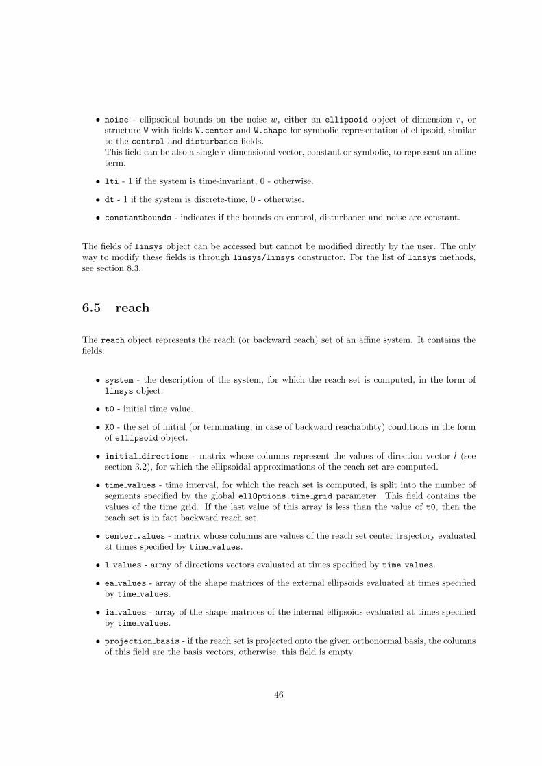
• noise - ellipsoidal bounds on the noise w, either an ellipsoid object of dimension r, orstructure W with fields W.center and W.shape for symbolic representation of ellipsoid, similarto the control and disturbance fields.This field can be also a single r-dimensional vector, constant or symbolic, to represent an affineterm.

• lti - 1 if the system is time-invariant, 0 - otherwise.

• dt - 1 if the system is discrete-time, 0 - otherwise.

• constantbounds - indicates if the bounds on control, disturbance and noise are constant.

The fields of linsys object can be accessed but cannot be modified directly by the user. The onlyway to modify these fields is through linsys/linsys constructor. For the list of linsys methods,see section 8.3.

6.5 reach

The reach object represents the reach (or backward reach) set of an affine system. It contains thefields:

• system - the description of the system, for which the reach set is computed, in the form oflinsys object.

• t0 - initial time value.

• X0 - the set of initial (or terminating, in case of backward reachability) conditions in the formof ellipsoid object.

• initial directions - matrix whose columns represent the values of direction vector l (seesection 3.2), for which the ellipsoidal approximations of the reach set are computed.

• time values - time interval, for which the reach set is computed, is split into the number ofsegments specified by the global ellOptions.time grid parameter. This field contains thevalues of the time grid. If the last value of this array is less than the value of t0, then thereach set is in fact backward reach set.

• center values - matrix whose columns are values of the reach set center trajectory evaluatedat times specified by time values.

• l values - array of directions vectors evaluated at times specified by time values.

• ea values - array of the shape matrices of the external ellipsoids evaluated at times specifiedby time values.

• ia values - array of the shape matrices of the internal ellipsoids evaluated at times specifiedby time values.

• projection basis - if the reach set is projected onto the given orthonormal basis, the columnsof this field are the basis vectors, otherwise, this field is empty.

46

• calc data - this field is empty unless the reach set is computed with the save all option setto 1. This field then contains the intermediate calculation data, which can be used for theapproximation refinement. For more detail, see description of the function refine in section8.4.

These fields can be accessed and modified only through reach methods. For the list of reachmethods, see section 8.4.

47

Chapter 7

Examples

7.1 Ellipsoids vs. Polytopes

Depending on the particular dynamical system, certain methods of reach set computation maybe more suitable than others. Even for a simple 2-dimensional discrete-time linear time-invariantsystem, application of ellipsoidal methods may be more effective than using polytopes.

Consider the system from chapter 1:[

x1[k + 1]x2[k + 1]

]=

[cos(1) sin(1)− sin(1) cos(1)

] [x1[k]x2[k]

]+

[u1[k]u2[k]

], x[0] ∈ X0, u[k] ∈ U, k ≥ 0,

where X0 is the set of initial conditions, and U is the control set.

Let X0 and U be unit boxes in R2, and compute the reach set using the polytope method implementedin MPT ([13]). With every time step the number of vertices of the reach set polytope increases by4. The complexity of the convex hull computation increases exponentially with number of vertices.In figure 7.1, the time required to compute the reach set for different time steps using polytopes isshown in red.

To compute the reach set of the system using Ellipsoidal Toolbox, we assume X0 and U to be unitballs in R2, fix any number of initial direction values that corresponds to the number of ellipsoidalapproximations, and obtain external and internal ellipsoidal approximations of the reach set:

>> A = [cos(1) sin(1); -sin(1) cos(1)];>> U = ell_unitball(2); % control bounds>>>> % define linear discrete-time system:>> lsys = linsys(A, eye(2), U, [], [], [], [], ’d’);>>>> X0 = ell_unitball(2); % set of initial conditions>> L0 = [cos(0:0.1:pi); sin(0:0.1:pi)]; % 32 initial directions>> N = 100; % number of time steps>>>> % compute the reach set:>> rs = reach(lsys, X0, L0, N);

48

In figure 7.1, the time required to compute both external and internal ellipsoidal approximations,with 32 ellipsoids each, for different number of time steps is shown in blue.

10 20 30 40 50 60 70 80 90 1000

20

40

60

80

100

120

140

160

180

200

Number of time steps

Rea

ch s

et c

ompu

tatio

n tim

e

ellipsoidspolytopes

Figure 7.1: Reach set computation performance comparison: ellipsoids (blue) vs. polytopes (red).

Figure 7.1 illustrates the fact that the complexity of polytope method grows exponentially withnumber of time steps, whereas the complexity of ellipsoidal method grows linearly.

7.2 System with Disturbance

The mechanical system presented in figure 7.2, is described by the following system of equations:

m1x1 + (k1 + k2)x1 − k2x2 = u1, (7.1)m2x2 − k2x1 + (k1 + k2)x2 = u2. (7.2)

Here u1 and u2 are the forces applied to masses m1 and m2, and we shall assume [u1 u2]T ∈ E(0, I).The initial conditions can be taken as x1(0) = 0, x2(0) = 2. Defining x3 = x1 and x4 = x2, we canrewrite (7.1-7.2) as a linear system in standard form:

x1

x2

x3

x4

=

0 0 1 00 0 0 1

−k1+k2m1

k2m1

0 0k2m2

−k1+k2m2

0 0

x1

x2

x3

x4

+

0 00 01

m10

0 1m2

[u1

u2

]. (7.3)

Now we can compute the reach set of system (7.1-7.2) for given time by computing the reach set ofthe linear system (7.3) and taking its projection onto (x1, x2) subspace.

>> % specify parameters k1, k2 and masses m1, m2:

49

m 1

m 2

x 1

x 2

k 1

k 1

k 2

u 1

u 2

Figure 7.2: Spring-mass system.

>> k1 = 24; k2 = 32;>> m1 = 1.5; m2 = 1;>>>> % define matrices A, B, and control bounds U:>> A = [0 0 1 0; 0 0 0 1; -(k1+k2)/m1 k2/m1 0 0; k2/m2 -(k1+k2)/m2 0 0];>> B = [0 0; 0 0; 1/m1 0; 0 1/m2];>> U = ell_unitball(2);>>>> lsys = linsys(A, B, U); % linear system>> T = [0 4]; % time interval>>>> % initial conditions:>> X0 = [0 2 0 0]’ + ellipsoid([0.01 0 0 0; 0 0.01 0 0; 0 0 eps 0; 0 0 0 eps]);>>>> % initial directions (some random vectors in R^4):>> L0 = [1 0 1 0; 1 -1 0 0; 0 -1 0 1; 1 1 -1 1 -1 1 1 0; -2 0 1 1]’;>>>> rs = reach(lsys, X0, L0, T); % reach set>>>> BB = [1 0 0 0; 0 1 0 0]’; % orthogonal basis of (x1, x2) subspace>> ps = projection(rs, BB); % reach set projection>>>> % plot projection of reach set external approximation:>> subplot(2, 2, 1);>> plot_ea(ps, ’g’); % plot the whole reach tube>> subplot(2, 2, 2);>> plot_ea(cut(ps, 4), ’g’); % plot reach set approximation at time t = 4

Figure 7.3(a) shows the reach set of the system (7.1-7.2) evolving in time from t = 0 to t = 4. Figure7.3(b) presents a snapshot of this reach set at time t = 4.

So far we considered an ideal system without any disturbance, such as friction. We introducedisturbance to (7.1-7.2) by adding extra terms, v1 and v2,

m1x1 + (k1 + k2)x1 − k2x2 = u1 + v1, (7.4)m2x2 − k2x1 + (k1 + k2)x2 = u2 + v2, (7.5)

50

Figure 7.3: Spring-mass system without disturbance: (a) reach tube for time t ∈ [0, 4]; (b) reach setat time t = 4. Spring-mass system with disturbance: (c) reach tube for time t ∈ [0, 4]; (d) reach setat time t = 4.

51

which results in equation (7.3) getting an extra term

0 00 01 00 1

[v1

v2

].

Assuming that [v1 v2]T is unknown but bounded by ellipsoid E(0, 14I), we can compute the closed-

loop reach set of the system with disturbance.

>> % define disturbance:>> G = [0 0; 0 0; 1 0; 0 1];>> V = 0.5*ell_unitball(2);>>>> lsysd = linsys(A, B, U, G, V); % linear system with disturbance>>>> rsd = reach(lsysd, X0, L0, T); % reach set>> psd = projection(rsd, BB); % reach set projection onto (x1, x2)>>>> % plot projection of reach set external approximation:>> subplot(2, 2, 3);>> plot_ea(ps); % plot the whole reach tube>> subplot(2, 2, 4);>> plot_ea(cut(ps, 4)); % plot reach set approximation at time t = 4

Figure 7.3(c) shows the reach set of the system (7.4-7.5) evolving in time from t = 0 to t = 4. Figure7.3(d) presents a snapshot of this reach set at time t = 4.

7.3 Switched System

By switched systems we mean systems whose dynamics changes at known times. Consider the RLCcircuit shown in figure 7.4. It has two inputs—the voltage (v) and current (i) sources. Define

• x1 - voltage across capacitor C1, so C1x1 is the corresponding current;

• x2 - voltage across capacitor C2, so the corresponding current is C2x2.

• x3 - current through the inductor L, so the voltage across the inductor is Lx3.

Applying Kirchoff current and voltage laws we arrive at the linear system,

x1

x2

x3

=

− 1

R1C10 − 1

C1

0 0 1C2

1L − 1

L −R2L

x1

x2

x3

+

1R1C1

1C1

0 00 0

[vi

]. (7.6)

The parameters R1, R2, C1, C2 and L, as well as the inputs, may depend on time. Suppose, fortime 0 ≤ t < 2, R1 = 2 Ohm, R2 = 1 Ohm, C1 = 3 F, C2 = 7 F, L = 2 H, both inputs, v and i are

52

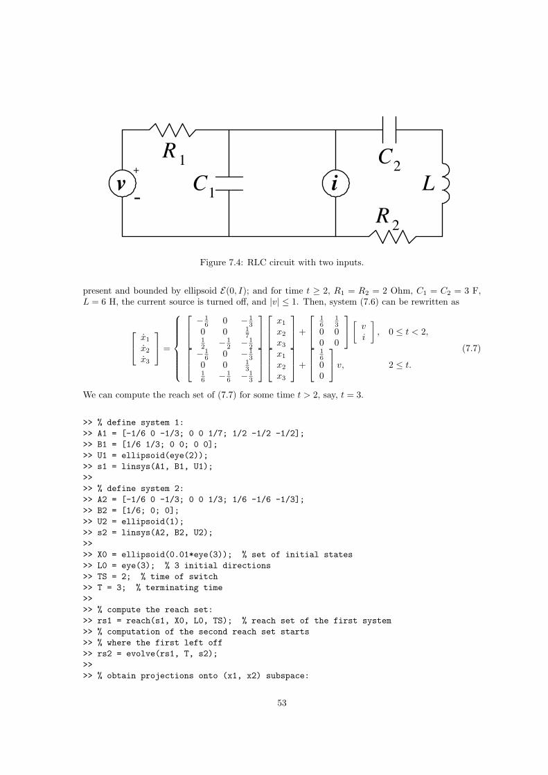
v i

R 1

R 2

C 1

C 2

L +

-

Figure 7.4: RLC circuit with two inputs.

present and bounded by ellipsoid E(0, I); and for time t ≥ 2, R1 = R2 = 2 Ohm, C1 = C2 = 3 F,L = 6 H, the current source is turned off, and |v| ≤ 1. Then, system (7.6) can be rewritten as

x1

x2

x3

=

− 1

6 0 − 13

0 0 17

12 − 1

2 − 12

x1

x2

x3

+

16

13

0 00 0

[vi

], 0 ≤ t < 2,

− 1

6 0 − 13

0 0 13

16 − 1

6 − 13

x1

x2

x3

+

1600

v, 2 ≤ t.

(7.7)

We can compute the reach set of (7.7) for some time t > 2, say, t = 3.

>> % define system 1:>> A1 = [-1/6 0 -1/3; 0 0 1/7; 1/2 -1/2 -1/2];>> B1 = [1/6 1/3; 0 0; 0 0];>> U1 = ellipsoid(eye(2));>> s1 = linsys(A1, B1, U1);>>>> % define system 2:>> A2 = [-1/6 0 -1/3; 0 0 1/3; 1/6 -1/6 -1/3];>> B2 = [1/6; 0; 0];>> U2 = ellipsoid(1);>> s2 = linsys(A2, B2, U2);>>>> X0 = ellipsoid(0.01*eye(3)); % set of initial states>> L0 = eye(3); % 3 initial directions>> TS = 2; % time of switch>> T = 3; % terminating time>>>> % compute the reach set:>> rs1 = reach(s1, X0, L0, TS); % reach set of the first system>> % computation of the second reach set starts>> % where the first left off>> rs2 = evolve(rs1, T, s2);>>>> % obtain projections onto (x1, x2) subspace:

53

>> BB = [1 0 0; 0 1 0]’; % (x1, x2) subspace basis>> ps1 = projection(rs1, BB);>> ps2 = projection(rs2, BB);>>>> % plot the results:>> subplot(2, 2, 1);>> plot_ea(ps1, ’r’); % external apprx. of reach set 1 (red)>> hold on;>> plot_ia(ps1, ’g’); % internal apprx. of reach set 1 (green)>> plot_ea(ps2, ’y’); % external apprx. of reach set 2 (yellow)>> plot_ia(ps2, ’b’); % internal apprx. of reach set 2 (blue)>>>> % plot the 3-dimensional reach set at time t = 3:>> subplot(2, 2, 2);>> plot_ea(cut(rs2, 3), ’y’);>> hold on;>> plot_ia(cut(rs2, 3), ’b’);

Figure 7.5(a) shows how the reach set projection onto (x1, x2) of system (7.7) evolves in time fromt = 0 to t = 3. The external reach set approximation for the first dynamics is in red, the internalapproximation is in green. The dynamics switches at t = 2. The external reach set approximationfor the second dynamics is in yellow, its internal approximation is in blue. The full three-dimensionalexternal (yellow) and internal (blue) approximations of the reach set are shown in figure 7.5(b).

To find out where the system should start at time t = 0 in order to reach a neighborhood M of theorigin at time t = 3, we compute the backward reach set from t = 3 to t = 0.

>> M = ellipsoid(0.01*eye(3)); % terminating set>> TT = 3; % terminating time>>>> % compute backward reach set:>> % compute the reach set:>> brs2 = reach(s2, M, L0, [TT TS]); % second system comes first>> brs1 = evolve(brs2, 0, s1); % then the first system>>>> % obtain projections onto (x1, x2) subspace:>> bps1 = projection(brs1, BB);>> bps2 = projection(brs2, BB);>>>> % plot the results:>> subplot(2, 2, 3);>> plot_ea(bps1, ’r’); % external apprx. of backward reach set 1 (red)>> hold on;>> plot_ia(bps1, ’g’); % internal apprx. of backward reach set 1 (green)>> plot_ea(bps2, ’y’); % external apprx. of backward reach set 2 (yellow)>> plot_ia(bps2, ’b’); % internal apprx. of backward reach set 2 (blue)>>>> % plot the 3-dimensional backward reach set at time t = 0:>> subplot(2, 2, 2);>> plot_ea(cut(brs1, 0), ’r’);

54

Figure 7.5: Forward and backward reach sets of the switched system (external and internal approx-imations). The dynamics switches at t = 2.(a) Forward reach set for the time interval 0 ≤ t ≤ 3 projected onto (x1, x2) subspace.(b) Forward reach set at t = 3 in R3.(c) Backward reach set evolving from t = 3 to t = 0 projected onto (x1, x2) subspace.(d) Backward reach set at t = 0 in R3.

55

>> hold on;>> plot_ia(cut(brs1, 0), ’g’);

Figure 7.5(c) presents the evolution of the reach set projection onto (x1, x2) in backward time.Again, external and internal approximations corresponding to the first dynamics are shown in redand green, and to the second dynamics in yellow and blue. The full dimensional backward reach setexternal and internal approximations of system (7.7) at time t = 0 is shown in figure 7.5(d).

7.4 Hybrid System

There is no explicit implementation of the reachability analysis for hybrid systems in the EllipsoidalToolbox. Nonetheless, the operations of intersection available in the toolbox allow us to work withcertain class of hybrid systems, namely, hybrid systems with affine continuous dynamics whoseguards are ellipsoids, hyperplanes, halfspaces or polytopes.

We consider the switching-mode model of highway traffic presented in [36]. The highway segment isdivided into N cells as shown in figure 7.6. In this particular case, N = 4. The traffic density in celli is xi vehicles per mile, i = 1, 2, 3, 4.

1 2 3 4

u 1

u 2

u 3

b

Figure 7.6: Highway model. Adapted from [36].

Define

• vi - average speed in mph, in the i-th cell, i = 1, 2, 3, 4;

• wi - backward congestion wave propagation speed in mph, in the i-th highway cell, i = 1, 2, 3, 4;

• xMi - maximum allowed density in the i-th cell; when this velue is reached, there is a trafficjam, i = 1, 2, 3, 4;

• di - length of i-th cell in miles, i = 1, 2, 3, 4;

• Ts - sampling time in hours;

• b - split ratio for the off-ramp;

56

• u1 - traffic flow coming into the highway segment, in vehicles per hour (vph);

• u2 - traffic flow coming out of the highway segment (vph);

• u3 - on-ramp traffic flow (vph).

Highway traffic operates in two modes: free-flow in normal operation; and congested mode, whenthere is a jam. Traffic flow in free-flow mode is described by

x1[t + 1]x2[t + 1]x3[t + 1]x4[t + 1]

=

1− v1Ts

d10 0 0

v1Ts

d21− v2Ts

d20 0

0 v2Ts

d31− v3Ts

d30

0 0 (1− b)v3Ts

d41− v4Ts

d4

x1[t]x2[t]x3[t]x4[t]

+

v1Ts

d10 0

0 0 v2Ts

d2

0 0 00 0 0

u1

u2

u3

. (7.8)

The equation for the congested mode is

x1[t + 1]x2[t + 1]x3[t + 1]x4[t + 1]

=

1− w1Ts

d1

w2Ts

d10 0

0 1− w2Ts

d2

w3Ts

d20

0 0 1− w3Ts

d3

11−b

w4Ts

d3

0 0 0 1− w4Ts

d4

x1[t]x2[t]x3[t]x4[t]

+

0 0 w1Ts

d1

0 0 00 0 00 −w4Ts

d40

u1

u2

u3

+

w1Ts

d1−w2Ts

d10 0

0 w2Ts

d2−w3Ts

d20

0 0 w3Ts

d3− 1

1−bw4Ts

d3

0 0 0 w4Ts

d4

xM1

xM2

xM3

xM4

. (7.9)

The switch from the free-flow to the congested mode occurs when the density x2 reaches xM2. Inother words, the hyperplane H([0 1 0 0]T , xM2) is the guard.

We indicate how to implement the reach set computation of this hybrid system. We first define thetwo linear systems and the guard.

>> % assign parameter values:>> v1 = 65; v2 = 60; v3 = 63; v4 = 65; % mph>> w1 = 10; w2 = 10; w3 = 10; w4 = 10; % mph>> d1 = 2; d2 = 3; d3 = 4; d4 = 2; % miles>> Ts = 2/3600; % sampling time in hours>> xM1 = 200; xM2 = 200; xM3 = 200; xM4 = 200; % vehicles per lane>> b = 0.4;>>>> A1 = [(1-(v1*Ts/d1)) 0 0 0

(v1*Ts/d2) (1-(v2*Ts/d2)) 0 0

57

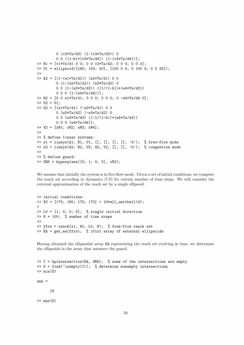
0 (v2*Ts/d3) (1-(v3*Ts/d3)) 00 0 ((1-b)*(v3*Ts/d4)) (1-(v4*Ts/d4))];

>> B1 = [v1*Ts/d1 0 0; 0 0 v2*Ts/d2; 0 0 0; 0 0 0];>> U1 = ellipsoid([180; 150; 50], [100 0 0; 0 100 0; 0 0 25]);>>>> A2 = [(1-(w1*Ts/d1)) (w2*Ts/d1) 0 0

0 (1-(w2*Ts/d2)) (w3*Ts/d2) 00 0 (1-(w3*Ts/d3)) ((1/(1-b))*(w4*Ts/d3))0 0 0 (1-(w4*Ts/d4))];

>> B2 = [0 0 w1*Ts/d1; 0 0 0; 0 0 0; 0 -w4*Ts/d4 0];>> U2 = U1;>> G2 = [(w1*Ts/d1) (-w2*Ts/d1) 0 0

0 (w2*Ts/d2) (-w3*Ts/d2) 00 0 (w3*Ts/d3) ((-1/(1-b))*(w4*Ts/d3))0 0 0 (w4*Ts/d4)];

>> V2 = [xM1; xM2; xM3; xM4];>>>> % define linear systems:>> s1 = linsys(A1, B1, U1, [], [], [], [], ’d’); % free-flow mode>> s2 = linsys(A2, B2, U2, G2, V2, [], [], ’d’); % congestion mode>>>> % define guard:>> GRD = hyperplane([0; 1; 0; 0], xM2);

We assume that initially the system is in free-flow mode. Given a set of initial conditions, we computethe reach set according to dynamics (7.8) for certain number of time steps. We will consider theexternal approximation of the reach set by a single ellipsoid.

>> initial conditions:>> X0 = [170; 180; 175; 170] + 10*ell_unitball(4);>>> L0 = [1; 0; 0; 0]; % single initial direction>> N = 100; % number of time steps>>>> ffrs = reach(s1, X0, L0, N); % free-flow reach set>> EA = get_ea(ffrs); % 101x1 array of external ellipsoids

Having obtained the ellipsoidal array EA representing the reach set evolving in time, we determinethe ellipsoids in the array that intersect the guard.

>> I = hpintersection(EA, GRD); % some of the intersections are empty>> D = find(~isempty(I)); % determine nonempty intersections>> min(D)

ans =

19

>> max(D)

58

ans =

69

Analyzing the values in array D, we conclude that the free-flow reach set has nonempty intersectionwith hyperplane GRD at t = 18 for the first time, and at t = 68 for the last time. Between t = 18 andt = 68 it crosses the guard. Figure 7.7(a) shows the free-flow reach set projection onto (x1, x2, x3)subspace for t = 10, before the guard crossing; figure 7.7(b) for t = 50, during the guard crossing;and figure 7.7(c) for t = 80, after the guard was crossed.

Figure 7.7: Reach set of the free-flow system is blue, reach set of the congested system is green, theguard is red.(a) Reach set of the free-flow system at t = 10, before reaching the guard (projection onto(x1, x2, x3)).(b) Reach set of the free-flow system at t = 50, crossing the guard. (projection onto (x1, x2, x3)).(c) Reach set of the free-flow system at t = 80, after the guard is crossed. (projection onto(x1, x2, x3)).(d) Reach set trace from t = 0 to t = 100, free-flow system in blue, congested system in green;bounds of initial conditions are marked with magenta (projection onto (x1, x2)).

For each time step that the intersection of the free-flow reach set and the guard is nonempty, weestablish a new initial time and a set of initial conditions for the reach set computation accordingto dynamics (7.9). The initial time is the array index minus one, and the set of initial conditions isthe intersection of the free-flow reach set with the guard.

59

>> crs = [];>> for i = 1:size(D, 2)

rs = reach(s2, I(D(i)), L0, [(D(i)-1) N]);crs = [crs rs];

end

The union of reach sets in array crs forms the reach set for the congested dynamics.

A summary of the reach set computation of the linear hybrid system (7.8-7.9) for N = 100 timesteps with one guard crossing is given in figure 7.7(d), which shows the projection of the reach settrace onto (x1, x2) subspace. The system starts evolving in time in free-flow mode from a set ofinitial conditions at t = 0, whose boundary is shown in magenta. The free-flow reach set evolvingfrom t = 0 to t = 100 is shown in blue. Between t = 18 and t = 68 the free-flow reach set crosses theguard. The guard is shown in red. For each nonempty intersection of the free-flow reach set and theguard, the congested mode reach set starts evolving in time until t = 100. All the congested modereach sets are shown in green. Observe that in the congested mode, the density x2 in the congestedpart decreases slightly, while the density x1 upstream of the congested part increases. The blue setabove the guard is not actually reached, because the state evolves according to the green region.

60

Chapter 8

Summary and Outlook

Although some of the operations with ellipsoids are present in the commercial Geometric BoundingToolbox [33, 34], the ellipsoid-related functionality of that toolbox is rather limited.

Ellipsoidal Toolbox is the first free MATLAB package that implements ellipsoidal calculus anduses ellipsoidal methods for reachability analysis of continuous- and discrete-time affine systems,continuous-time linear systems with disturbances and switched systems, whose dynamics changes atknown times. The reach set computation for hybrid systems whose guards are hyperplanes or poly-hedra is not implemented explicitly, but the tool for such computation exists, namely, the operationsof intersection of ellipsoid with hyperplane and ellipsoid with halfspace.

In future versions of the toolbox we intend to implement additional operations with ellipsoids:

• external and internal ellipsoidal approximations of the intersection of N ellipsoids (currently,these operations are implemented only for N = 2);

• external and internal ellipsoidal approximations for the sets

(E1 ⊕ E2)−E3 and E1 ⊕ (E2−E3),(E1 ⊕ E2) ∩ E3 and (E1−E2) ∩ E3;

• ordering of ellipsoids: partial ordering of their shape matrices;

• ellipsoidal approximations of non-ellipsoidal convex sets, e.g. polytopes;

• reachability analysis for state-constrained and obstacle problems; and

• ellipsoidal methods for stochastic control and estimation.

61

Acknowledgement

The authors would like to thank Alexander B. Kurzhanski, Manfred Morari, Johan Lofberg, MichalKvasnica and Goran Frehse for their support of this work by useful advice and encouragement.

62

Bibliography

[1] Ellipsoidal Toolbox homepage: www.eecs.berkeley.edu/˜akurzhan/ellipsoids

[2] A.B.Kurzhanski, I.Valyi (1997). Ellipsoidal Calculus for Estimation and Control. Birkhauser,Boston, ser. SCFA.

[3] A.B.Kurzhanski, P.Varaiya (2000). On ellipsoidal techniques for reachability analysis. In: Op-timization Methods and Software, Vol.17, pp.177-237, Taylor & Francis.

[4] A.B.Kurzhanski, P.Varaiya (2002). On reachability under uncertainty, In SIAM Journal onControl and Optimization, Vol.41(1), pp.181-216.

[5] A.B.Kurzhanski, P.Varaiya (2001). Reachability analysis for uncertain systems - the ellipsoidaltechnique. In: Dynamics of Continuous, Discrete and Impulsive Systems Series B: Applicationsand Algorithms, Vol.9, pp.347-367.

[6] A.A.Kurzhanskiy, P.Varaiya (2005). Ellipsoidal Techniques for Reachability Analysis ofDiscrete-Time Linear Systems. Submitted to IEEE Transactions on Automatic Control.

[7] P.Varaiya (1998). Reach set computation using optimal control. In: Proc. of KIT Workshop onVerification on Hybrid Systems. Verimag, Grenoble.

[8] P.Varaiya. Lecture notes on optimization. (www.eecs.berkeley.edu/˜varaiya/papers ps.dir/NOO.pdf).

[9] A.Yu.Vazhentsev (1999). On Internal Ellipsoidal Approximations for Problems of Control Syn-thesis with Bounded Coordinates. In: Izvestia Rossiiskoi Akademii Nauk. Teoriya i SystemyUpravleniya.

[10] L.Ros, A.Sabater, F.Thomas (2002). An Ellipsoidal Calculus Based on Propagation and Fusion.In: IEEE Transactions on Systems, Man and Cybernetics - Part B: Cybernetics, Vol.32, N.4.

[11] Robust Ellipsoidal Calculus homepage: www-iri.upc.es/people/ros/ellipsoids.html

[12] M.Kvasnica, P.Grieder, M.Baotic, M.Morari (2004). Multi-Parametric Toolbox (MPT). In:R.Alur and G.J.Pappas, editors, Hybrid Systems: Computation and Control, Vol.2993 of Lec-ture Notes in Computer Science, pp.448-462. Springer-Verlag.

[13] Multi-Parametric Toolbox homepage: control.ee.ethz.ch/˜mpt

[14] J.Lofberg (2004). A Toolbox for Modeling and Optimization in MATLAB. In: Proceedings ofCACSD Conference, Taipei, Taiwan.

[15] YALMIP homepage: control.ee.ethz.ch/˜joloef/yalmip.php.

63

[16] J.F.Sturm (1999). Using SeDuMi 1.02, A MATLAB Toolbox for Optimization over SymmetricCones. In: Optimization Methods and Software, Vol.11-12, pp.625-653, Taylor & Francis.

[17] SeDuMi homepage: sedumi.mcmaster.ca

[18] I.Mitchell, C.Tomlin (2000). Level set methods for computation in hybrid systems, In: N.Lynchand B.H.Krogh, editors, Hybrid Systems: Computation and Control, Vol.1790 of Lecture Notesin Computer Science. Springer-Verlag.

[19] Level Set Toolbox homepage: www.cs.ubc.ca/˜mitchell/ToolboxLS

[20] O.Stursberg, B.H.Krogh (2003). Efficient representation and computation of reachable sets forhybrid systems, In: O.Maler and A.Pnueli, editors, Hybrid Systems: Computation and Control,Vol.2623 of Lecture Notes in Computer Science, pp.482-497. Springer-Verlag.

[21] CheckMate homepage: www.ece.cmu.edu/˜webk/checkmate

[22] E.Asarin, O.Bournez, T.Dang, O.Maler (2000). Approximate reachability analysis of piecewiselinear dynamical systems, In: N.Lynch and B.H.Krogh, editors, Hybrid Systems: Computationand Control, Vol.1790 of Lecture Notes in Computer Science, pp.21-31. Springer-Verlag.

[23] d/dt homepage: www-verimag.imag.fr/˜tdang/ddt.html

[24] A.Girard (2005). Reachability of uncertain linear systems using zonotopes. In: M.Morari andL.Thiele, editors, Hybrid Systems: Computation and Control, Vol.3414 of Lecture Notes inComputer Science, pp 291-305. Springer-Verlag.

[25] A.Girard, C.Le Guernic, O.Maler (2006). Computation of reachable sets of linear time-invariant systems with inputs, In: J.Hespanha and A.Tiwari, editors, Hybrid Systems: Com-putation and Control, Vol.3927 of Lecture Notes in Computer Science, pp.257-271. Springer-Verlag.

[26] MATISSE homepage: www.seas.upenn.edu/˜agirard/Software/MATISSE

[27] Zonotope methods on Wolfgang Kuhn homepage: www.decatur.de

[28] T.S.Motzkin, H.Raiffa, G.L.Thompson, R.M.Thrall (1953). The Double Description Method.In: H.W.Kuhn and A.W.Tucker, editors, Conttributions to theory of games, Vol.2. PrincetonUniversity Press.

[29] CDD/CDD+ homepage: www.cs.mcgill.ca/˜fukuda/soft/cdd home/cdd.html

[30] D.Avis, D.Bremner, R.Seidel (1997). How good are convex hull algorithms? In: ComputationalGeometry: Theory and Applications No.7, pp.265-301. ELSEVIER.

[31] G.Lafferriere, G.J.Pappas, S.Yovine (2001). Symbolic Reachability Computation for Familiesof Linear Vector Fields. In: Journal of Symbolic Computation No.32, pp.231-253, AcademicPress.

[32] Requiem homepage: www.seas.upenn.edu/˜hybrid/requiem/requiem.html

[33] S.M.Veres, A.V.Kuntsevich, I.Valyi, S.Hermsmeyer, D.S.Wall (2001). Geometric Boundingtoolbox for MATLAB. In: MATLAB/Simulink Connections Catalogue. Natick, MA: Math-Works Inc.

[34] Geometric Bounding Toolbox homepage: www.sysbrain.com/gbt

64

[35] E.K.Kostousova (2001). Control synthesis via parallelotopes: optimization and parallel compu-tations. In: Optimization Methods and Software, Vol.14, N.4, pp.267-310, Taylor & Francis.

[36] L.Munoz, X.Sun, R.Horowitz, L.Alvarez (2003). Traffic density estimation with the cell trans-mission model, In: Proceedings of the American Control Conference, Denver, Colorado, USA,pp.3750-3755.

[37] S.Boyd, L.El Ghaoui, E.Feron, V.Balakrishnan (1994). Linear Matrix Inequalities in Systemand Control Theory. SIAM.

[38] S.Boyd, L.Vandenberghe (2004). Convex Optimization. Cambridge University Press.

[39] F.R.Gantmacher (1960). Matrix theory, I-II. Chelsea Pub., NY.

[40] G.H.Golub, C.F.Van Loan (1996). Matrix Computations, 3rd Edn. The Johns Hopkins Uni-versity Press.

[41] R.T.Rockafellar (1999). Convex Analysis, 2nd Edn. Princeton University Press.

65

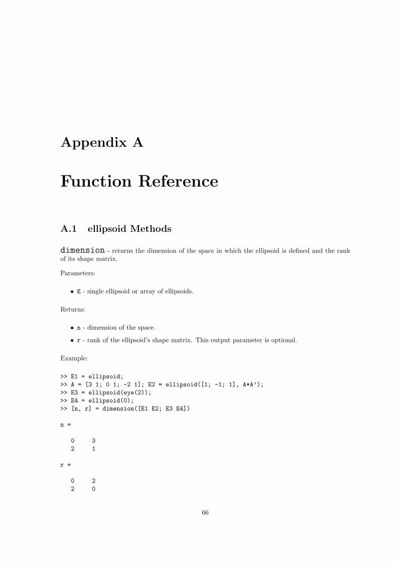
Appendix A

Function Reference

A.1 ellipsoid Methods

dimension - returns the dimension of the space in which the ellipsoid is defined and the rankof its shape matrix.

Parameters:

• E - single ellipsoid or array of ellipsoids.

Returns:

• n - dimension of the space.

• r - rank of the ellipsoid’s shape matrix. This output parameter is optional.

Example:

>> E1 = ellipsoid;>> A = [3 1; 0 1; -2 1]; E2 = ellipsoid([1; -1; 1], A*A’);>> E3 = ellipsoid(eye(2));>> E4 = ellipsoid(0);>> [n, r] = dimension([E1 E2; E3 E4])

n =

0 32 1

r =

0 22 0

66

display - displays the details of the ellipsoid object.

Parameters:

• E - ellipsoid or array of ellipsoids.

This function is rarely used explicitely. It is called automatically for the object E when semicolondoes not terminate the statement.

67

distance - computes the distance from the given ellipsoid to the specified object - vector,ellipsoid, hyperplane or polytope.

Parameters:

• E - ellipsoid or array of ellipsoids.

• X - in case of vectors, it is a matrix, whose columns represent the vectors to which the distanceis measured, number of columns must match the number of ellipsoids in the array E;in case of ellipsoids, it is array of ellipsoids whose size must match the size of E;in case of hyperplanes, it is array of hyperplanes whose size must match the size of E;in case of polytopes, it is polytope array whose length must match the number of ellipsoids inthe array E.

• F - this flag if set to 1 indicates that the distance should be computed in the metric of ellipsoidsin E. This parameter is optional, its default value is 0, and the distance is computed in theEuclidean metric. This parameter makes no difference for the distance computation betweenellipsoids and polytopes.

Returns:

• D - distance or array of distances.

Example:

>> E = ellipsoid([-2; -1], [4 -1; -1 1]);>> V = [1 1; 1 -1; -1 1; -1 -1]’;>> distance(E, V)

ans =

1.0000 -1.0000 1.6668 1.0855

68

ellipsoid - constructor for the ellipsoid object. If called without parameters, returns emptyellipsoid.

Parameters:

• q - center of the ellipsoid, vector in Rn. This parameter is optional, and if omitted, it isassumed that the ellipsoid is centered at the origin.

• Q - shape matrix of the ellipsoid, matrix in Rn×n, symmetric positive semidefinite.

Returns:

• E - object of type ellipsoid class.

Example:

>> E = ellipsoid([1 0 -1 6]’, 9*eye(4));

creates a ball of radius 3 in R4 centered at [1 0 − 1 6]T .

69

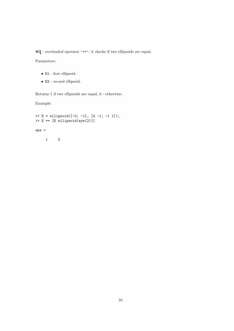
eq - overloaded operator ’==’, it checks if two ellipsoids are equal.

Parameters:

• E1 - first ellipsoid.

• E2 - second ellipsoid.

Returns 1 if two ellipsoids are equal, 0 - otherwise.

Example:

>> E = ellipsoid([-2; -1], [4 -1; -1 1]);>> E == [E ellipsoid(eye(2))]

ans =

1 0

70

ge, gt - checks if the first ellipsoid is bigger than the second one.

Parameters:

• E1 - first ellipsoid.

• E2 - second ellipsoid.

Returns 1 if E1 contains E2 when both have the same center, 0 - otherwise.

Example:

>> E > E

ans =

1

illustrates the fact that an ellipsoid is always bigger than itself.

71

hpintersection - computes the ellipsoid which results from intersection of given ellipsoidwith given hyperplane.

Parameters:

• E - ellipsoid or array of ellipsoids.

• H - hyperplane or array of hyperplanes.

If E and H are arrays, then their sizes must match.

Returns:

• I - ellipsoid or array of ellipsoids that are intersections of ellipsoids in E with hyperplanes in H.

Example:

>> E = ellipsoid([-2; -1], [4 -1; -1 1]);>> H = [hyperplane([0 -1; -1 0]’, 1); hyperplane([0 1; 1 0]’, 1)];>> I = hpintersection(E, H)

I =2x2 array of ellipsoids.

72

intersect - checks if the union or intersection of ellipsoids intersects given ellipsoid, hyperplaneor polytope.

Parameters:

• E - ellipsoid or array of ellipsoids whose union or intersection is considered.

• X - can be single or array of ellipsoids, hyperplanes or polytopes.

• s - if ’u’, E should be treated as union of ellipsoids, if ’i’, E should be treated as intersectionof ellipsoids. This parameter is optional, its default value is ’u’.

Returns −1 in case parameter s is set to ’i’ and the intersection of ellipsoids in E is empty,0 if the union or intersection of ellipsoids in E does not intersect the object in X,1 if the union or intersection of ellipsoids in E and the object in X have nonempty intersection.

Example:

>> E1 = ellipsoid([-2; -1], [4 -1; -1 1]);>> E2 = E1 + [5; 5];>> H = hyperplane([1; -1]);>> intersect([E1 E2], H)

ans =

1

>> intersect([E1 E2], H, ’i’)

ans =

-1

Here two ellipsoids E1 and E2 do not intersect but both are intersected by hyperplane H.

73

intersection ea - computes the external ellipsoidal approximation of the intersection of theellipsoid with given ellipsoid, halfspace or polytope.

Parameters:

• E - ellipsoid or array of ellipsoids.

• X - can be single or array of ellipsoids, hyperplanes or polytopes.

If E and X are arrays, then their sizes must match.

Returns:

• EA - ellipsoid or array of ellipsoids that externally approximate the intersection.

Example:

>> E1 = ellipsoid([-2; -1], [4 -1; -1 1]);>> E2 = E1 + [5; 5];>> B = ell_unitball(2);>> EA = intersection_ea([E1 E2], B)

EA =1x2 array of ellipsoids.

74

intersection ia - computes the internal ellipsoidal approximation of the intersection of theellipsoid with given ellipsoid, halfspace or polytope.

Parameters:

• E - ellipsoid or array of ellipsoids.

• X - can be single or array of ellipsoids, hyperplanes or polytopes.

If E and X are arrays, then their sizes must match.

Returns:

• IA - ellipsoid or array of ellipsoids that internally approximate the intersection.

Example:

>> E1 = ellipsoid([-2; -1], [4 -1; -1 1]);>> E2 = E1 + [5; 5];>> B = ell_unitball(2);>> IA = intersection_ia([E1 E2], B)

IA =1x2 array of ellipsoids.

75

inv - inverts the shape matrix of the ellipsoid if it is nonsingular.

Parameters:

• E - ellipsoid or array of ellipsoids.

Returns:

• I - ellipsoid or array of ellipsoids with inverted shape matrices.

76

isbaddirection - checks if ellipsoidal approximations of the geometric difference of twoellipsoids can be computed for given directions.

Parameters:

• E1 - first ellipsoid.

• E2 - second ellipsoid.

• L - matrix whose columns are direction vectors that need to be checked.

Returns 1 if given direction is bad and ellipsoidal approximation cannot be computed for it, 0 -otherwise.

Example:

>> E = ellipsoid([-2; -1], [4 -1; -1 1]);>> B = 3*ell_unitball(2);>> L = [1 0; 1 1; 0 1; -1 1]’;>> isbaddirection(B, E, L)

ans =

0 1 1 0}

means that for vectors [1 1]T and [0 1]T the ellipsoidal approximation of the geometric differenceB−E cannot be computed.

77

isdegenerate - checks if given ellipsoid is degenerate.

Parameters:

• E - ellipsoid or array of ellipsoids.

Returns 1 if the ellipsoid is degenerate, 0 - otherwise.

78

isempty - checks if given ellipsoid is an empty object.

Parameters:

• E - ellipsoid or array of ellipsoids.

Returns 1 if empty, 0 - otherwise.

79

isinside - checks if the intersection of ellipsoids contains the union or intersection of givenellipsoids or polytopes.

Parameters:

• E - ellipsoid or array of ellipsoids whose intersection contains or not the union or intersectionof other given objects.

• X - can be array of ellipsoids or polytopes whose union or intersection belongs or not to theintersection E.

• s - if ’u’, X should be treated as union, if ’i’, X should be treated as intersection. Thisparameter is optional, its default value is ’u’.

Returns −1 if parameter s is set to ’i’ and the intersection of ellipsoids or polytopes in X is empty,0 - if the intersection E does not cover X,1 - if E contains X.

Example:

>> E = ellipsoid([-2; -1], [4 -1; -1 1]);>> B = ell_unitball(2);>> isinside(E, [E B], ’i’)

ans =

1

illustrates the fact that any ellipsoid contains its intersection with another ellipsoid.

80

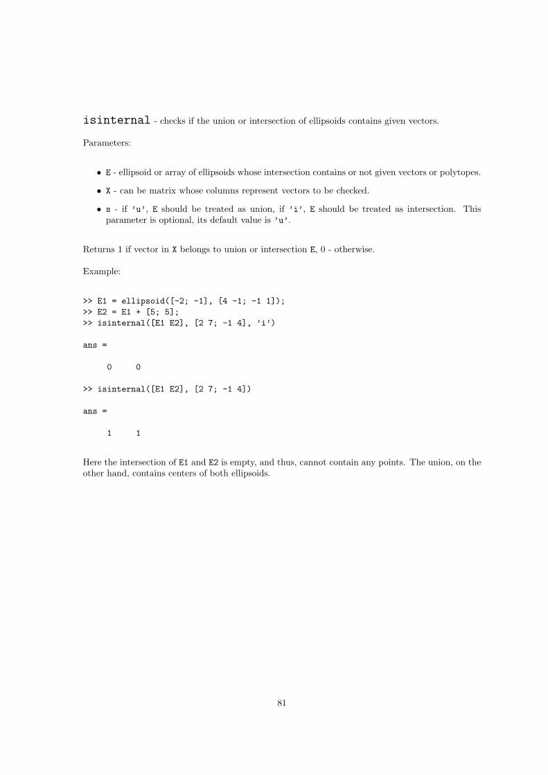
isinternal - checks if the union or intersection of ellipsoids contains given vectors.

Parameters:

• E - ellipsoid or array of ellipsoids whose intersection contains or not given vectors or polytopes.

• X - can be matrix whose columns represent vectors to be checked.

• s - if ’u’, E should be treated as union, if ’i’, E should be treated as intersection. Thisparameter is optional, its default value is ’u’.

Returns 1 if vector in X belongs to union or intersection E, 0 - otherwise.

Example:

>> E1 = ellipsoid([-2; -1], [4 -1; -1 1]);>> E2 = E1 + [5; 5];>> isinternal([E1 E2], [2 7; -1 4], ’i’)

ans =

0 0

>> isinternal([E1 E2], [2 7; -1 4])

ans =

1 1

Here the intersection of E1 and E2 is empty, and thus, cannot contain any points. The union, on theother hand, contains centers of both ellipsoids.

81

le, lt - checks if the second ellipsoid is bigger than the first one.

Parameters:

• E1 - first ellipsoid.

• E2 - second ellipsoid.

Returns 1 if E2 contains E1 when both have the same center, 0 - otherwise.

This operation is the mirror of ge, gt.

82

maxeig - returns the biggest eigenvalue of the ellipsoid.

Parameters:

• E - ellipsoid or array of ellipsoids.

Returns:

• a - largest eigenvalue or array of largest eigenvalues of ellipsoids in E.

83

mineig - returns the smallest eigenvalue of the ellipsoid.

Parameters:

• E - ellipsoid or array of ellipsoids.

Returns:

• a - smallest eigenvalue or array of smallest eigenvalues of ellipsoids in E.

84

minkdiff - computes and plots the geometric difference of two ellipsoids in 2D and 3D.

Parameters:

• E1 - first ellipsoid.

• E2 - second ellipsoid.

• o - options structure whose fields describe how the geometric difference must be plotted. Thefields of this structure are

– show all - if set to 1, also displays the ellipsoids E1 and E2;

– newfigure - if set to 1, each plot command will open a new figure window;

– fill - if set to 1, the resulting set and the ellipsoids, if plotted in 2D, will be filled withcolor;

– color - specifies the color of the plot in the RGB format: [x y z];

– shade - the level of transparency for 3D plots, takes values between 0 and 1 (0 - trans-parent, 1 - opaque).

This parameter is optional.

Returns:

• x - center of the resulting set.

• X - matrix whose columns represent the boundary points of the resulting set. The number ofpoints is defined by parameters plot2d grid for 2D plots and plot3d grid for 3D plots of theglobal ellOptions structure.

Both output parameters are optional.

85

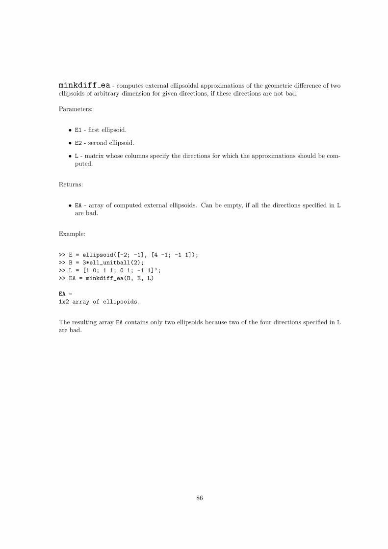
minkdiff ea - computes external ellipsoidal approximations of the geometric difference of twoellipsoids of arbitrary dimension for given directions, if these directions are not bad.

Parameters:

• E1 - first ellipsoid.

• E2 - second ellipsoid.

• L - matrix whose columns specify the directions for which the approximations should be com-puted.

Returns:

• EA - array of computed external ellipsoids. Can be empty, if all the directions specified in Lare bad.

Example:

>> E = ellipsoid([-2; -1], [4 -1; -1 1]);>> B = 3*ell_unitball(2);>> L = [1 0; 1 1; 0 1; -1 1]’;>> EA = minkdiff_ea(B, E, L)

EA =1x2 array of ellipsoids.

The resulting array EA contains only two ellipsoids because two of the four directions specified in Lare bad.

86

minkdiff ia - computes internal ellipsoidal approximations of the geometric difference of twoellipsoids of arbitrary dimension for given directions, if these directions are not bad.

Parameters:

• E1 - first ellipsoid.

• E2 - second ellipsoid.

• L - matrix whose columns specify the directions for which the approximations should be com-puted.

Returns:

• EA - array of computed internal ellipsoids. Can be empty, if all the directions specified in L arebad.

Example:

>> E = ellipsoid([-2; -1], [4 -1; -1 1]);>> B = 3*ell_unitball(2);>> L = [1 0; 1 1; 0 1; -1 1]’;>> IA = minkdiff_ia(B, E, L)

IA =1x2 array of ellipsoids.

The resulting array IA contains only two ellipsoids because two of the four directions specified in Lare bad.

87

minksum - computes and plots the geometric sum of finite number of ellipsoids in 2D and 3D.

Parameters:

• E - array of ellipsoids whose geometric sum needs to be computed.

• o - options structure whose fields describe how the geometric sum must be plotted. The fieldsof this structure are

– show all - if set to 1, also displays the ellipsoids in the array E;

– newfigure - if set to 1, each plot command will open a new figure window;

– fill - if set to 1, the resulting set and the ellipsoids, if plotted in 2D, will be filled withcolor;

– color - specifies the color of the plot in the RGB format: [x y z];

– shade - the level of transparency for 3D plots, takes values between 0 and 1 (0 - trans-parent, 1 - opaque).

This parameter is optional.

Returns:

• x - center of the resulting set.

• X - matrix whose columns represent the boundary points of the resulting set. The number ofpoints is defined by parameters plot2d grid for 2D plots and plot3d grid for 3D plots of theglobal ellOptions structure.

Both output parameters are optional.

88

minksum ea - computes external ellipsoidal approximations of the geometric sum of finite num-ber of ellipsoids of arbitrary dimension for given directions.

Parameters:

• E - array of ellipsoids whose geometric sum needs to be approximated.

• L - matrix whose columns specify the directions for which the approximations should be com-puted.

Returns:

• EA - array of computed external ellipsoids whose length is the same as the number of columnsof matrix L.

Example:

>> E = ellipsoid([-2; -1], [4 -1; -1 1]);>> B = ell_unitball(2);>> L = [1 0; 1 1; 0 1; -1 1]’;>> EA = minkdiff_ea([E B inv(E)] L)

EA =1x4 array of ellipsoids.

89

minksum ia - computes internal ellipsoidal approximations of the geometric sum of finite numberof ellipsoids of arbitrary dimension for given directions.

Parameters:

• E - array of ellipsoids whose geometric sum needs to be approximated.

• L - matrix whose columns specify the directions for which the approximations should be com-puted.

Returns:

• IA - array of computed internal ellipsoids whose length is the same as the number of columnsof matrix L.

Example:

>> E = ellipsoid([-2; -1], [4 -1; -1 1]);>> B = ell_unitball(2);>> L = [1 0; 1 1; 0 1; -1 1]’;>> IA = minkdiff_ia([E B inv(E)] L)

IA =1x4 array of ellipsoids.

90

minus - overloaded operator ’-’.

Parameters:

• E - ellipsoid or array of ellipsoids defined in Rn.

• b - vector in Rn or matrix in Rn×m, where m equals the number of ellipsoids in the array E.

Returns:

• E1 - ellipsoid or array of ellipsoids with same shapes as E, but with centers shifted by vectorsin -b.

Example:

>> E = [ellipsoid([-2; -1], [4 -1; -1 1]) ell_unitball(2)];>> E1 = E - [1; 1];>> E1(1)

ans =

Center:-3-2

Shape:4 -1

-1 1

Nondegenerate ellipsoid in R^2.

>> E1(2)

ans =

Center:-1-1

Shape:1 00 1

Nondegenerate ellipsoid in R^2.

91

move2origin - moves given ellipsoids to the origin.

Parameters:

• E - ellipsoid or array of ellipsoids.

Returns:

• O - the same ellipsoid or array of ellipsoids as E, but all centered at the origin.

Example:

>> E = ellipsoid([-2; -1], [4 -1; -1 1]);>> O = move2origin(E)

O =

Center:00

Shape:4 -1

-1 1

Nondegenerate ellipsoid in R^2.

92

mtimes - overloaded operator ’*’.

Parameters:

• A - scalar, or matrix in Rm×n.

• E - ellipsoid or array of ellipsoids defined in Rn.

Returns:

• E1 - ellipsoid or array of ellipsoids resulting from linear transformation of E.

Example:

>> E = ellipsoid([-2; -1], [4 -1; -1 1]);>> A = [0 1; -1 0];>> A*E

ans =

Center:-12

Shape:1 11 4

Nondegenerate ellipsoid in R^2.

93

ne - overloaded operator ’~=’, it checks if two ellipsoids are not equal.

Parameters:

• E1 - first ellipsoid.

• E2 - second ellipsoid.

Returns 1 if two ellipsoids are not equal, 0 - otherwise.

Example:

>> E = ellipsoid([-2; -1], [4 -1; -1 1]);>> E \~{ }= [E ellipsoid(eye(2))]

ans =

0 1

94

parameters - returns parameters of the ellipsoid, its center and shape matrix.

Parameters:

• E - single ellipsoid.

Returns:

• q - center of the ellipsoid. It is optional output parameter.

• Q - shape matrix of the ellipsoid.

95

plot - plots ellipsoids in 1D, 2D and 3D.

Parameters:

• E - ellipsoid or array of ellipsoids.

• c - specifies the color:

– ’b’ - blue;

– ’c’ - cyan;

– ’g’ - green;

– ’k’ - black;

– ’m’ - magenta;

– ’r’ - red;

– ’w’ - white;

– ’y’ - yellow.

This parameter is optional.

• o - options structure whose fields describe how the ellipsoids must be plotted. The fields ofthis structure are

– newfigure - if set to 1, each plot command will open a new figure window;

– fill - if set to 1, the resulting set and the ellipsoids, if plotted in 2D, will be filled withcolor;

– width - specifies line width for 1D and 2D plots;

– color - specifies the color of the plot in the RGB format: [x y z];

– shade - the level of transparency for 3D plots, takes values between 0 and 1 (0 - trans-parent, 1 - opaque).

This parameter is optional.

Returns: None.

96

plus - overloaded operator ’+’.

Parameters:

• E - ellipsoid or array of ellipsoids defined in Rn.

• b - vector in Rn or matrix in Rn×m, where m equals the number of ellipsoids in the array E.

Returns:

• E1 - ellipsoid or array of ellipsoids with same shapes as E, but with centers shifted by vectorsin b.

Example:

>> E = [ellipsoid([-2; -1], [4 -1; -1 1]) ell_unitball(2)];>> E1 = E + [1; 1];>> E1(1)

ans =

Center:-10

Shape:4 -1

-1 1

Nondegenerate ellipsoid in R^2.

>> E1(2)

ans =

Center:11

Shape:1 00 1

Nondegenerate ellipsoid in R^2.

97

polar - computes polars for ellipsoids which contain the origin.

Parameters:

• E - ellipsoid or array of ellipsoids.

Returns:

• P - polar ellipsoid or array of polar ellipsoids for those in E.

For ellipsoids that do not contain the origin, this function returns empty ellipsoid.

Example:

>> E = ellipsoid([4 -1; -1 1]);>> polar(E) == inv(E)

ans =

1

illustrates the fact that polar set of an ellipsoid centered at the origin equals to inverse of thisellipsoid.

98

projection - computes projection of ellipsoids onto given orthogonal basis.

Parameters:

• E - ellipsoid or array of ellipsoids defined in Rn.

• B - matrix in Rn×m whose columns are orthogonal.

Returns:

• P - array of projected ellipsoids.

Example:

>> E = ellipsoid([-2; -1; 4], [4 -1 0; -1 1 0; 0 0 9]);>> B = [0 1 0; 0 0 1]’;>> P = projection(E, B)

P =

Center:-14

Shape:1 00 9

Nondegenerate ellipsoid in R^2.

99

rho - computes the support function of the ellipsoids for given directions and corresponding bound-ary points.

Parameters:

• E - ellipsoid or array of ellipsoids defined in Rn.

• L - vector in Rn if E is an array of ellipsoids, otherwise, if E is a single ellipsoid, it can bematrix in Rn×m whose columns represent the directions for which the support function needsto be computed.

Returns:

• R - array of support function values.

• X - matrix whose columns are boundary points corresponding to the directions in L. Thisoutput parameter is optional.

100

shape - has the same functionality as mtimes but modifies only the shape matrix of the ellipsoidleaving its center as is.

Parameters:

• A - scalar, or matrix in Rm×n.

• E - ellipsoid or array of ellipsoids defined in Rn.

Returns:

• E1 - ellipsoid or array of ellipsoids resulting from modification of the shape matrices of ellipsoidsin E.

Example:

>> E = ellipsoid([-2; -1], [4 -1; -1 1]);>> A = [0 1; -1 0];>> shape(E, A)

ans =

Center:-2-1

Shape:1 11 4

Nondegenerate ellipsoid in R^2.

101

uminus - overloaded operation unitary minus.

Parameters:

• E - ellipsoid or array of ellipsoids.

Returns:

• E1 - array of the same ellipsoids as in E, whose centers are multilied by −1.

Example:

>> E = -ellipsoid([-2; -1], [4 -1; -1 1])

E =

Center:21

Shape:4 -1

-1 1

Nondegenerate ellipsoid in R^2.

102

volume - computes volume of given ellipsoids.

Parameters:

• E - ellipsoid or array of ellipsoids.

Returns:

• V - array of volume values whose size matches the size of E.

Example:

>> E = ellipsoid([-2; -1], [4 -1; -1 1]);>> B = ell_unitball(2);>> V = volume([E B])

V =

5.4414 3.1416

103

A.2 hyperplane Methods

contains - checks if the hyperplanes contain given vectors.

Parameters:

• H - hyperplane or array of hyperplanes.

• X - matrix whose columns represent the vectors needed to be checked. The number of columnsmust match the number of hyperplanes in H.

Returns 1 if the vector in X belongs to the hyperplane in H, 0 - otherwise.

Example:

>> H = hyperplane([-1; 1]);>> X = [100 -1 2; 100 1 2];>> contains(H, X)

ans =

1 0 1

104

dimension - returns the dimension of the space in which the hyperplane is defined.

Parameters:

• H - hyperplane or array of hyperplanes.

Returns:

• D - array of dimension values of the same size as H.

Example:

>> H1 = hyperplane([-1; 1]);>> H2 = hyperplane([-1; 1; 8; -2; 3], 7);>> H3 = hyperplane([1; 2; 0], -1);>> D = dimension([H1 H2 H3]);

D =

2 5 3

105

display - displays the details of the hyperplane object.

Parameters:

• H - hyperplane or array of hyperplanes.

This function is rarely used explicitely. It is called automatically for the object H when semicolondoes not terminate the statement.

106

eq - overloaded operator ’==’. it checks if two hyperplanes are equal.

Parameters:

• H1 - first hyperplane.

• H2 - second hyperplane.

Returns 1 if two hyperplanes are equal, 0 - otherwise.

Example:

>> H1 = hyperplane([-1; 1]);>> H2 = hyperplane([-1; 1; 8; -2; 3], 7);>> H3 = hyperplane([1; 2; 0], -1);>> H2 == [H1 H2 H3]

ans =

0 1 0

107

hyperplane - constructor for the hyperplane object. If called without parameters, returnsempty hyperplane.

Parameters:

• V - vector in Rn or matrix in Rn×m whose columns define the normals to the hyperplanes thatneed to be created.

• C - scalar value, or, in case V has m columns, it can be array with m values.

Returns:

• H - hyperplane, or, if V has more than one column, array of hyperplanes.

Example:

>> V = [1 1 1; 1 1 1];>> C = [1 -5 0];>> H = hyperplane(V, C);

defines three parallel hyperplanes and returns them in the array H.

108

isempty - checks if the hyperplane object is empty.

Parameters:

• H - hyperplane or array of hyperplanes.

Returns: 1 if the hyperplane object is empty, 0 - otherwise.

109

isparallel - checks if the hyperplanes are parallel.

Parameters:

• H1 - first hyperplane.

• H2 - second hyperplane.

Returns 1 if two hyperplanes are equal, 0 - otherwise.

Example:

>> H = hyperplane([-1 1; 1 1; 1 1], [2 1 0]);>> isparallel(H, H(2))

ans =

0 1 1

110

ne - overloaded operator ’~=’, it checks if two hyperplanes are not equal.

Parameters:

• H1 - first hyperplane.

• H2 - second hyperplane.

Returns 1 if two hyperplanes are not equal, 0 - otherwise.

Example:

>> H1 = hyperplane([-1; 1]);>> H2 = hyperplane([-1; 1; 8; -2; 3], 7);>> H3 = hyperplane([1; 2; 0], -1);>> [H2 H1 H3] == [H1 H2 H3]

ans =

0 0 1

111

parameters - returns parameters of the hyperplane object, its normal and scalar.

Parameters:

• H - hyperplane object.

Parameters:

• v - normal vector.

• c - scalar. This output parameter is optional.

112

plot - plots hyperplanes in 2D and 3D.

Parameters:

• H - hyperplane or array of hyperplanes.

• c - specifies the color:

– ’b’ - blue;

– ’c’ - cyan;

– ’g’ - green;

– ’k’ - black;

– ’m’ - magenta;

– ’r’ - red;

– ’w’ - white;

– ’y’ - yellow.

This parameter is optional.

• o - options structure whose fields describe how the hyperplanes must be plotted. The fields ofthis structure are

– newfigure - if set to 1, each plot command will open a new figure window;

– size - length of the line segment in 2D or square diagonal in 3D.

– center - center of the line segment in 2D or square diagonal in 3D.

– width - specifies line width for 2D plots;

– color - specifies the color of the plot in the RGB format: [x y z];

– shade - the level of transparency for 3D plots, takes values between 0 and 1 (0 - trans-parent, 1 - opaque).

This parameter is optional.

Returns: None.

113

uminus - overloaded operator unitary minus. It does not change the hyperplane, and affects onlythe halfspace this hyperplane defines.

Parameters:

• H - hyperplane or array of hyperplanes.

Returns:

• H1 - array of the same hyperplanes as in H whose normals and scalars are multiplied by −1.

Example:

>> H = -hyperplane([-1; 1], 1)

H =

Normal:1

-1

Shift:-1

Hyperplane in R^2.

114

A.3 linsys Methods

dimension - returns dimensions of state, input, output and disturbance input spaces.

Parameters:

• LSYS - linear system or array of linear systems.

Returns:

• N - state space dimension.

• I - dimension of the input space.

• O - dimension of the output space.

• D - dimension of the disturbance input space.

115

display - displays the details of the linear system object.

Parameters:

• LSYS - linear system or array of linear systems.

This function is rarely used explicitely. It is called automatically for the object LSYS when semicolondoes not terminate the statement.

116

hasdisturbance - checks if given linear system is the system with disturbance.

Parameters:

• LSYS - linear system or array of linear systems.

Returns 1 if it is system with disturbance, 0 - otherwise.

117

hasnoise - checks if given linear system has noise at the output.

Parameters:

• LSYS - linear system or array of linear systems.

Returns 1 if it is system with noise, 0 - otherwise.

118

isdiscrete - checks if given linear system is discrete-time.

Parameters:

• LSYS - linear system or array of linear systems.

Returns 1 if the system is discrete-time, 0 - otherwise.

119

isempty - checks if given linear system is an empty object.

Parameters:

• LSYS - linear system or array of linear systems.

Returns 1 if LSYS is an empty object, 0 - otherwise.

120

islti - checks if given linear system is time invariant.

Parameters:

• LSYS - linear system or array of linear systems.

Returns 1 if the system is time invariant, 0 - otherwise.

121

linsys - constructor for the linear system object. If called without parameters, creates an emptyobject.

Parameters:

• A - matrix A ∈ Rn×n, can be symbolic if it depends on time (t - in continuous case, k - indiscrete case).

• B - matrix B ∈ Rn×m, can by symbolic if it depends on time.

• U - defines control bounds: it can be ellipsoid object with dimension m; or structure with fieldscenter - symbolic vector, and shape - symbolic matrix, if the ellipsoidal bounds depend ontime; or, if the control is fixed, it can be single vector of type double or symbolic.

• G - matrix G ∈ Rn×d, can by symbolic if it depends on time. This parameter is optional.

• V - defines disturbance bounds: it can be ellipsoid object with dimension d; or structure withfields center - symbolic vector, and shape - symbolic matrix, if the ellipsoidal bounds dependon time; or, if the control is fixed, it can be single vector of type double or symbolic. Thisparameter is optional.

• C - matrix C ∈ Ro×n, can by symbolic if it depends on time. This parameter is optional.

• W - defines noise bounds: it can be ellipsoid object with dimension o; or structure with fieldscenter - symbolic vector, and shape - symbolic matrix, if the ellipsoidal bounds depend ontime; or, if the control is fixed, it can be single vector of type double or symbolic. Thisparameter is optional.

• s - if set to ’d’, indicates that the system is discrete-time.

Returns:

• LSYS - linear system object.

Example:

>> A = {’0’ ’1 + cos(pi*k/2)’; ’-2’ ’0’};>> B = [0; 1];>> U = ellipsoid(4);>> G = [1; 0];>> V = 1/(k+1);>> C = [1 0];>> lsys = linsys(A, B, U, G, V, C, [], ’d’);

defines the following affine discrete-time system:[

x1[k + 1]x2[k + 1]

]=

[0 1 + cos(πk

2 )−2 0

]+

[01

]u[k] +

[1

k+1

0

], − 2 ≤ u[k] ≤ 2

y[k] = [1 0][

x1[k]x2[k]

], k ≥ 0.

122

A.4 reach Methods

cut - extracts a segment of the reach tube from the given start time to the given end time.

Parameters:

• RS - reach set object.

• T - time interval of interest in the form [t1 t2]. If T is a single scalar, then the reach set forthis particular time value is returned.

Returns:

• CRS - the resulting reach set object.

123

dimension - returns the dimension of the reach set and the dimension of the state space forwhich the reach set was originally computed.

Parameters:

• RS - reach set object.

Returns:

• d - dimension of the reach set.

• n - dimension of the state space for which the reach set was originally computed. Values ofd and n can be different if the reach set object is a result of projection operation. Thisparameter is optional.

124

display - displays the details of the reach set object.

Parameters:

• RS - reach set object.

This function is rarely used explicitely. It is called automatically for the object LSYS when semicolondoes not terminate the statement.

125

evolve - computes further evolution in time of the already existing reach set.

Parameters:

• CRS - existing reach set.

• T - new time horizon.

• LSYS - linear system object that describes new dynamics. This parameter is optional.

Returns:

• RS - reach set object.

126

get center - returns trajectory of the center of the reach set.

Parameters:

• RS - reach set object.

Returns:

• X - matrix whose columns represent the position of the center at times specified in the secondoutput parameter, T.

• T - array of time values at which the trajectory of the reach set center is evaluated. Thisoutput parameter is optional.

The number of columns in X and values in T is specified by the parameter time grid of theellOptions structure.

127

get directions - returns the trajectories of the direction vectors for which the ellipsoidalapproximations were computed.

Parameters:

• RS - reach set object.

Returns:

• X - array of cells where each cell represents a trajectory of the direction vector, for which theellipsoidal approximations of the reach set were computed.

• T - array of time values at which these trajectories are evaluated. This output parameter isoptional.

The number of columns in cells of X and values in T is specified by the parameter time grid of theellOptions structure.

128

get ea - returns array of ellipsoids that represent the external approximation of the reach set.

Parameters:

• RS - reach set object.

Returns:

• E - array of ellipsoids that externally approximate the reach set. The intersection of ellipsoidsin the given column of this array is the external approximation of the reach set at the timespacified by the corresponding value in the array T.

• T - array of time values at which the approximations are evaluated. This output parameter isoptional.

The number of columns in E and values in T is specified by the parameter time grid of theellOptions structure.

129

get goodcurves - returns the trajectories along which the ellipsoidal approximations aretouching the actual reach set.

Parameters:

• RS - reach set object.

Returns:

• X - array of cells where each cell represents a good trajectory along which one of the computedellipsoidal approximations touches the reach set.

• T - array of time values at which the good trajectories are evaluated. This output parameteris optional.

The number of columns in cells of X and values in T is specified by the parameter time grid of theellOptions structure.

130

get ia - returns array of ellipsoids that represent the internal approximation of the reach set.

Parameters:

• RS - reach set object.

Returns:

• E - array of ellipsoids that internally approximate the reach set. The union of ellipsoids in thegiven column of this array is the internal approximation of the reach set at the time specifiedby the corresponding value in the array T.

• T - array of time values at which the approximations are evaluated. This output parameter isoptional.

The number of columns in E and values in T is specified by the parameter time grid of theellOptions structure.

131

get system - returns the linear system object for which the reach set was computed.

Parameters:

• RS - reach set object.

Returns:

• LSYS - the linear system object, which was used for the reach set computation.

132

intersect - checks if the external or internal approximation of the reach set intersects withgiven ellipsoids, hyperplanes or polytopes.

Parameters:

• RS - reach set object.

• X - can be array of ellipsoids, hyperplanes or polytopes.

• s - if set to ’i’, indicates that internal approximation should be checked, if set to ’e’ -external. This input parameter is optional, its default value is ’e’.

Returns 1 if the intersection is nonempty, 0 - otherwise.

133

iscut - checks if the given reach set object resulted from cut operation.

Parameters:

• RS - reach set object.

Returns 1 if RS is a result of cut operation, 0 - otherwise.

134

isempty - checks if the given reach set object is empty.

Parameters:

• RS - reach set object.

Returns 1 if it is an empty object, 0 - otherwise.

135

isprojection - checks if the given reach set is a result of projection operation.

Parameters:

• RS - reach set object.

Returns 1 if RS is a projection, 0 - otherwise.

136

plot ea - plots external approximation of the reach set in 2D and 3D.

Parameters:

• RS - reach set object.

• c - specifies the color:

– ’b’ - blue;

– ’c’ - cyan;

– ’g’ - green;

– ’k’ - black;

– ’m’ - magenta;

– ’r’ - red;

– ’w’ - white;

– ’y’ - yellow.

This parameter is optional.

• o - options structure whose fields describe how the reach set must be plotted. The fields ofthis structure are

– width - specifies line width for 2D plots;

– fill - if set to 1, the set, if plotted in 2D, will be filled with color;

– color - specifies the color of the plot in the RGB format: [x y z];

– shade - the level of transparency for 3D plots, takes values between 0 and 1 (0 - trans-parent, 1 - opaque).

This parameter is optional.

Returns: None.

137

plot ia - plots internal approximation of the reach set in 2D and 3D.

Parameters:

• RS - reach set object.

• c - specifies the color:

– ’b’ - blue;

– ’c’ - cyan;

– ’g’ - green;

– ’k’ - black;

– ’m’ - magenta;

– ’r’ - red;

– ’w’ - white;

– ’y’ - yellow.

This parameter is optional.

• o - options structure whose fields describe how the reach set must be plotted. The fields ofthis structure are

– width - specifies line width for 2D plots;

– fill - if set to 1, the set, if plotted in 2D, will be filled with color;

– color - specifies the color of the plot in the RGB format: [x y z];

– shade - the level of transparency for 3D plots, takes values between 0 and 1 (0 - trans-parent, 1 - opaque).

This parameter is optional.

Returns: None.

138

projection - projects the reach set onto the given orthogonal basis.

Parameters:

• RS - reach set object with dimension n.

• B - matrix in Rn×m whose columns are orthogonal, they represent the basis vectors.

Returns:

• PRS - reach set object with the projected reach set.

139

reach - constructor for the reach set object and the main function that computes the reach set.

Parameters:

• LSYS - the linear system object with state space dimension n.

• X0 - ellipsoid object with dimension n, it represents the set of initial conditions.

• L0 - matrix in Rn×m whose columns represent the directions for which the new approximationsneed to be computed.

• T - time interval in the form [t0 t1]. If t1 is smaller than t0, then the backward reach setshould be computed. If T is a scalar, then it is assumed that t0 = 0.

• o - options structure with fields

– approximation - if set to 0, then only external approximation is computed, if set to1, then only internal approximation is computed, if set to 2 (default value), then bothapproximations are computed.

– save all - if set to 0 (default value), then the intermediate calculation data should notbe saved, 1indicates the opposite.

This parameter is optional.

Returns:

• RS - reach set object.

140

refine - adds new approximations for the specified directions to the given reach set object, thusimproving the overall approximation.

Parameters:

• RS - reach set object with dimension n. This object must contain the intermediate calculationdata, otherwise, the refinement is not possible.

• L0 - matrix in Rn×m whose columns represent the directions for which the new approximationsneed to be computed.

• o - options structure with fields

– approximation - if set to 0, then only external approximation is computed, if set to1, then only internal approximation is computed, if set to 2 (default value), then bothapproximations are computed.

– save all - if set to 0, then the intermediate calculation data should not be saved, 1(default value) indicates the opposite.

This parameter is optional.

Returns:

• RRS - reach set object with refined approximation.

141

A.5 Miscellaneous Functions

ell simdiag - computes the orthogonal transformation matrix that simultaneously diagonal-izes two symmetric matrices.

Parameters:

• A - symmetric positive definite matrix in Rn×n.

• B - symmetric positive semidefinite matrix in Rn×n.

Returns:

• T - orthogonal matrix in Rn×n, such that TATT is identity matrix, and TBTT is diagonalmartrix.

142

ell unitball - creates the ellipsoid object that represents a unit ball of the given dimension.

Parameters:

• n - dimension of the space in which the unit ball is defined.

Returns:

• B - ellipsoid object with identity shape matrix centered at the origin.

143

ell valign - computes the orthogonal matrix that aligns two vectors.

Parameters:

• w - vector in Rn.

• v - vector in Rn that needs to be rotated to be parallel to w.

Returns:

• S - orthogonal matrix in Rn×n, such that Sv = ‖v‖2‖w‖2 w.

144

hyperplane2polytope - converts array of hyperplanes of the same dimension into thepolytope object of the Multi-Parametric Toolbox.

Parameters:

• H - array of hyperplanes, all of which must have the same dimension.

Returns:

• P - polytope object as defined in the Multi-Parametric Toolbox.

145

polytope2hyperplane - converts the polytope object of the Multi-Parametric Toolbox intothe array of hyperplanes.

Parameters:

• P - polytope object as defined in the Multi-Parametric Toolbox.

Returns:

• H - array of hyperplanes.

146