Embed Size (px)
Citation preview

P. v;o43 ' CONTRACTOR REPORT
d
SAND93 - 7028 Unlimited R e l e a s e UC-252
eliminary Study of Disc aracteristics of Slim H duction Wells in Liquid-Dom thermal Reservoirs
! ~ John W. Pritchett ' I PO Box 1620 I La Jolla, CA 92038-1620
S-CUBED
Prepared by Sandia National Laboratories Albuquerque, New Mexico 87185 and Livermore, California 94550 for the United States Department of Energy under Contract DE-AC04-76DP00789
'
~ Pr in ted June 1993

Issued by Sandia National Laboratories, operated for the United States Department of Energy by Sandia Corporation. NOTICE: This report was prepared as an account of work sponsored by an agency of the United States Government. Neither the United States Govern- ment nor any agency thereof, nor any of their employees, nor any of their contractors, subcontractors, or their employees, makes any warranty, express or implied, or assumes any legal liability or responsibility for the accuracy, completeness, or usefulness of any information, apparatus, product, or process disclosed, or represents that its use would not infringe privately owned rights. Reference herein to any specific commercial product, process, or service by trade name, trademark, manufacturer, or otherwise, does not necessarily constitute or imply its endorsement, recommendation, or favoring by the United States Government, any agency thereof or any of their contractors or subcontractors. The views and opinions expressed herein do not necessarily state or reflect those of the United States Government, any agency thereof or any of their contractors.
Printed in the United States of America. This report has been reproduced directly from the best available copy.
Available to DOE and DOE contractors from Office of Scientific and Technical Information PO Box 62 Oak Ridge, T N 37831
Prices available from (615) 576-8401, FTS 626-8401
Available to the public from National Technical Information Service US Department of Commerce 5285 Port Royal Rd Springfield, VA 22161
NTIS price codes Printed copy: A04 Microfiche copy: A01

DISCLAIMER Portions of this document may be illegible in electronic image products. Images are produced from the best available original document.

SAND93-7028 Unlimited Release Printed June 1993
Distribution Category UC-2 5 2
Preliminary Study of Discharge Characteristics of Slim Holes
Compared to Production Wells in Liquid-Dom inated
G eo the rm a I Reservoirs
John W. Pritchett
P.O. Box 1620 La Jolla, CA 92038-1 620
S-CUBED
Abstract
There is current interest in using slim holes for geothermal exploration and reservoir assessment. A major question that must be addressed is whether results from flow or injection testing of slim holes can be scaled to predict large diam$ter production well performance. This brief report describes a preliminary examination of this question from a purely theoretical point of view. The WELBOR computer program was used to perform a ser ies of calculations of the steady flow of fluid up geothermal boreholes of various diameters at various discharge rates. Starting with prescribed bottom hole conditions (pressure, enthalpy), the WELBOR code integrates the equations expressing conservation of mass, momentum and energy (together with fluid constitutive properties obtained from’ the steam tables) upwards towards the wellhead using numerical techniques. This results in computed profiles of conditions (pressure, temperature, steam volume fraction, etc.) as functions of depth within the flowing well, and also in a forecast of wellhead conditions (pressure, temperature, enthalpy, etc.). From these results, scaling rules are developed and discussed.

c This work was supported through Geo Hills
Associates under Contract AA- 71 44 from Sandia National Laboratories. The author thanks James Dunn, Charles Hickok, Roger Eaton, Sabodh Garg, and Jim Combs for their reviews and comments on this report.
Acknowledgment
.. 11

TABLE OF CONTENTS
Section Page
.. Acknowledgment ...................................................................................................................... 11
List of Figures .......................................................................................................................... iv
List of Tables ............................................................................................................................ vi
1 . Introduction ...................................................................................................................... 1
2 . Results Neglecting Reservoir Flow Resistance ................................................................ 3
3 . The Influence of Pipe Friction ......................................................................................... 6
4 .
5 .
6 .
7 .
8 .
9 .
10 .
11 .
The Influence of Heat Losses ........................................................................................... 9
The Difficulty of Initiating Slim-Hole Discharge .......................................................... 19
Incorporation of Reservoir Flow Resistance .................................................................. 24
Estimation of Productivity Index: Cylindrical Flow Approximation .............................. 25
Estimation of Productivity Index: Spherical Flow Approximation ............................... 28
Results for Finite Reservoir Flow Resistance ................................................................ 31
Conclusions and Recommendations ............................................................................... 42
References ...................................................................................................................... 44
I
I I
Appendix
A . Mathematical Formulation of Two-Phase Fluid Flow in a Wellbore .......................... A- 1

LIST OF FIGURES
Figure
1
2
3
4
10
, 1 la
Influence of borehole diameter on borehole performance characteristics (no reservoir flow resistance). ............................................................................................................ 4
Maximum discharge rate (at one bar absolutewellhead pressure) as function of borehole diameter in the absence of reservoir flow resistance (bottomhole flowing pressure = 80 bars absolute). ......................................................................................... 7
Minimum discharge rate (at one bar absolute wellhead pressure) as function of borehole diameter in the absence of reservoir flow resistance (bottomhole flowing pressure = 80 bars absolute). ........................................................................................ 10
Typical flowing conditions in production well. Note that reservoir flow resistance is assumed to be zero (bottomhole flowing pressure = 80 bars). Dotted line indicates formation temperature profile. .................................................................................... 12
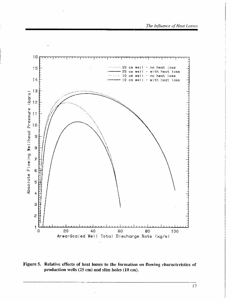
Relative effects of heat losses to the formation on flowing characteristics of production wells (25 cm) and slim holes (10 cm). ...................................................... 17
Effective heat transfer coefficient multiplier as a function of time after flow startup for various values of borehole diameter (centimeters). ............................................... 20
Ranges of area-scaled discharge rate within which discharge is possible for IO-cm slim holes and 25-cm production wells, for various values of heat loss multiplier. Reservoir flow resistance neglected (flowing bottomhole pressure = 80 bars). ......... 21
Time required for heat loss multiplier to drop to 114 of critical value for 10-cm diameter slim holes and 25-cm diameter production wells. ........................................ 23
Productivity index scaling exponent (p) for various drainage radii (rD) and skin factor (S) values. .................................................................................................................... 27
Productivity index scaling exponent (p) under various conditions based on results reported by Tang (1 988). ................................................................................. 30
Wellhead pressure as function of area-scaled well discharge rate for slim hole (10 cm diameter) and production well (25 cm diameter) with no reservoir flow resistance. .. 35
~ I iv

_. _ ..... ........................
List of Figures
Figure
1 lb
1 IC
1 Id
1 le
1 If
Page
Wellhead pressure as function of area-scaled well discharge rate for slim hole (10 cm diameter) and production well (25 cm diameter) with production-well productivity index equal to 6 kilograms per second per bar. ........................................................... 36
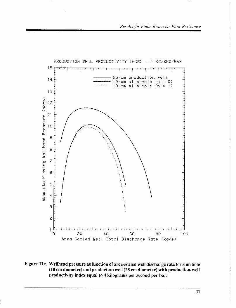
Wellhead pressure as function of area-scaled well discharge rate for slim hole (10 cm diameter) and production well (25 cm diameter) with production-well productivity index equal to 4 kilograms per second per bar. ........................................................... 37
Wellhead pressure as function of area-scaled well discharge rate for slim hole (10 cm diameter) and production well (25 cm diameter) with production-well productivity index equal to 3 kilograms per second per bar. ........................................................... 38
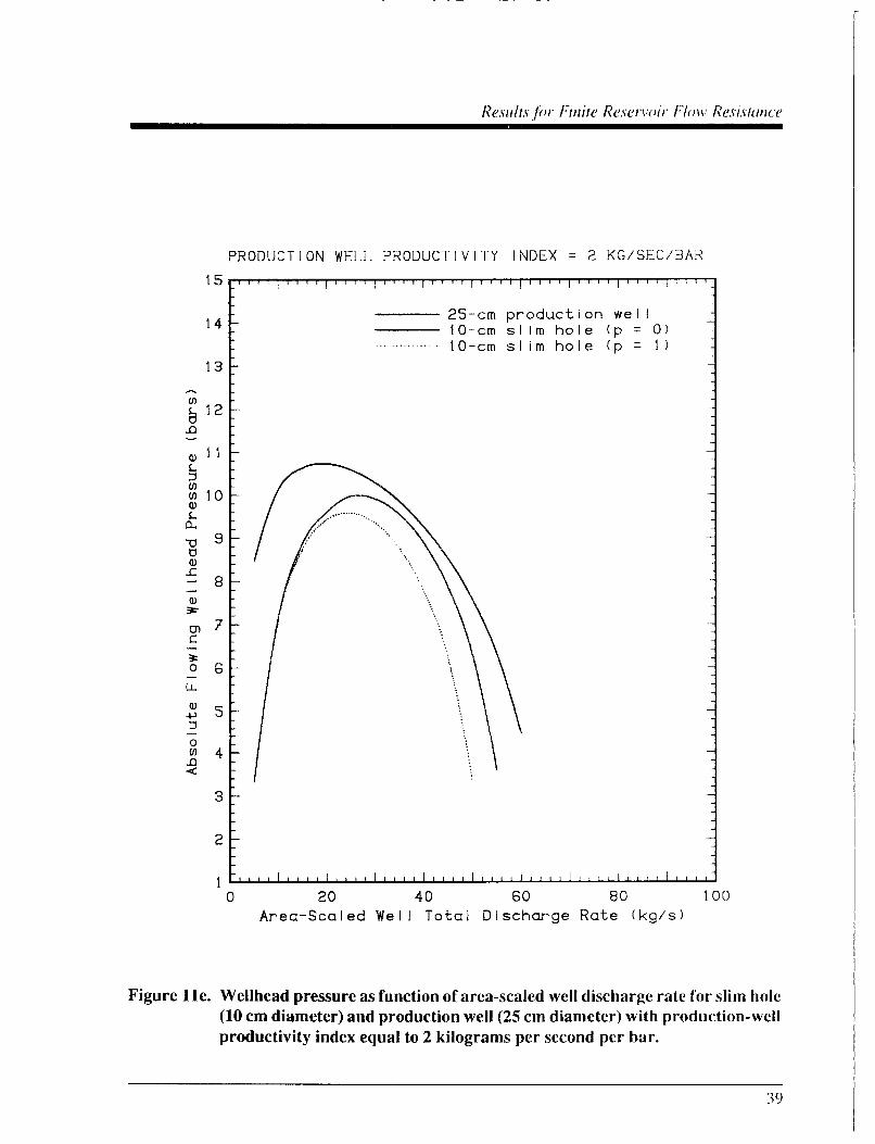
Wellhead pressure as function of area-scaled well discharge rate for slim hole (10 cm diameter) and production well (25 cm diameter) with production-well productivity index equal to 2 kilograms per second per bar. ........................................................... 39
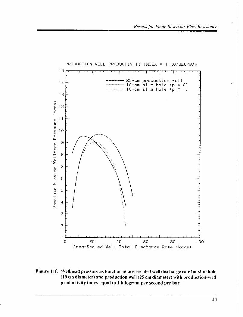
Wellhead pressure as function of area-scaled well discharge rate for slim hole (10 cm diameter) and production well (25 cm diameter) with production-well productivity index equal to 1 kilogram per second per bar. ............................................................ 40

LIST OF TABLES
Table Page
1
2
3
4
5
6
7
8
9
10
Reservoir temperature distribution assumed for WELBOR calculations. .................... 2
Wellhead pressure as a function of borehole diameter (0) and area-scaled discharge rate (M*) neglecting flow resistance of reservoir (bottomhole pressure = 80 bars). .... 5
Maximum discharge rate as function of borehole diameter for no reservoir flow resistance. .............................................................................................................. 8
Minimum discharge rate as function of borehole diameter for no reservoir flow resistance. ............................................................................................................ 11
Wellhead fluid enthalpy decrease (relative to bottomhole flowing enthalpy) as a function of borehole diameter (D) and area-scaled discharge rate (M*) neglecting flow resistance of reservoir (bottomhole pressure = 80 bars). ................................... .13
-
Increase in fluid kinetic energy from bottomhole to wellhead as function of discharge rate for slim hole and production well. ....................................................... 14
Influence of heat loss to formation on production well and slim hole performance. ................................................................................................................ 18
Performance characteristics of 25-cm diameter production well as a function of productivity index. ...................................................................................................... 32
Performance characteristics of 10-cm diameter slim hole using p = 0 productivity index scaling rule. ................................................................................... 33
Performance characteristics of IO-cm diameter slim hole using p = 1 productivity index scaling rule. ................................................................................... 34
vi

1. INTRODUCTION
During the exploration of a geothermal prospect, so-called ‘‘slim holes” offer an attractive alternative to full-size production well drilling for preliminary characterization of the reservoir, owing both to lower cost and reduced drilling time requirements. The most important problem in reservoir exploration is to establish the underground temperature distribution and the presence of a thermal resource, and large-diameter wells at not required for downhole temperature measurements. Slim holes can also serve to help characterize geological structure, and many geothermal well logging tools can be run in relatively small-diameter holes.
8 The fluid discharge capacity of a typical slim hole will generally be significantly less than
that of a comsponding production-size hole, however. This means, of course, that if a productive region is discovered using slim-hole exploration, it will be necessary to subsequently drill production- size wells to exploit the resource. ..so, due to their relatively low fluid discharge capacity, slim holes are not usually useful as signal sources for pressure interference testing (they may, however, be used as shut-in observation wells in interference tests in which the flowing wells are of conventional diameter).
If a slim hole is drilled into a geothermal prospect and can be induced to discharge, the rate of steam production from the slim hole is presumably much less than would have occurred had the well been of conventional diameter. Accordingly, one question of interest is how one might estimate the steam delivery capacity of future production-size wells based upon results h m testing slim holes. The discharge characteristics of a geothermal well involve the relationships among stable wellhead flowing pressure, total mass discharge rate, and wellhead fluid enthalpy @e., steadwater ratio). If these characteristics are known for one or more slim holes in a prospective geothermal field, is it possible to estimate the corresponding characteristics of future production wells in any meaningful way?
This brief report describes a preliminary examination of this question from a purely theoretical point of view. The WELBOR computer program (Pntchett, 1985, see Appendix A) was used to perform a series of calculations of the steady flow of .fluid up geothermal boreholes of various diameters at various discharge rates. Starting with prescribed bottomhole conditions (pressure, enthalpy), the WELBOR code integrates the equations expressing conservation of mass, momentum and energy (together with fluid constitutive properties obtained from the steam tables) upwards towards the wellhead using numerical techniques. This results in computed profiles of conditions (pressure, temperature, steam volume fraction, etc.) as functions of depth within the flowing well, and also in a forecast of wellhead conditions (pressure, temperature, enthalpy, etc.). Pipe friction (for both single- and two-phase flow regions) is treated using the formulation of Dukler, Wicks and Cleveland (1964). Liquid holdup (that is, the relative motion between the liquid and vapor phases) is treated using Hughmark’s (1962) correlation. Heat transfer through the casing between the fluid
I
I
I
I I
1
. . . . - . . . . . - . . . . . . . . . . . - . . - . . . . . . . . . . . . . . . .. . . . . - . . . .. . . - - . . . . . . . . . .
I Introduction
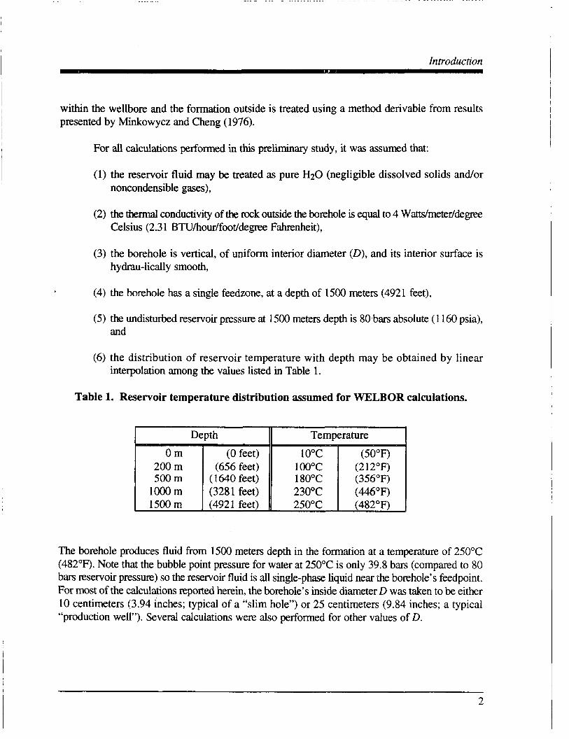
within the wellbore and the formation outside is treated using a method derivable from results presented by Minkowycz and Cheng (1976).
For all calculations performed in this preliminary study, it was assumed that:
(1) the reservoir fluid may be treated as pure H20 (negligible dissolved solids and/or noncondensible gases),
(2) the thermal conductivity of the rock outside the borehole is equal to 4 Watts/meter/degree Celsius (2.3 I BTU/hour/foot/degree Fahrenheit),
(3) the borehole is vertical, of uniform interior diameter (D), and its interior surface is hydrau-lically smooth,
(4) the borehole has a single feedzone, at a depth of 1500 meters (4921 feet),
(5) the undisturbed reservoir pressure at 1500 meters depth is 80 bars absolute (1 160 psia), and
(6) the distribution of reservoir temperature with depth may be obtained by linear interpolation among the values listed in Table 1.
Table 1. Reservoir temperature distribution assumed for WELBOR calculations.
Depth II Temperature
(0 feet) (50°F) (656 feet) (212°F)
500 m (1640 feet) 180°C (356°F) (3281 feet)
The borehole produces fluid from 1500 meters depth in the formation at a temperature of 250°C (482OF). Note that the bubble point pressure for water at 250°C is only 39.8 bars (compared to 80 bars reservoir pressure) so the reservoir fluid is all single-phase liquid near the borehole’s feedpoint. For most of the calculations reported herein, the borehole’s inside diameter D was taken to be either 10 centimeters (3.94 inches; typical of a “slim hole”) or 25 centimeters (9.84 inches; a typical “production well”). Several calculations were also performed for other values of D.
2

2. RESULTS NEGLECTING RESERVOIR FLOW RESISTANCE
It is first instructive to examine the fluid carrying capacity of the well as a function of borehole diameter without consideration of the resistance of the reservoir to fluid discharge. Therefore, for this first series of calculations, it was assumed that the bottomhole flowing pressure is the same as the reservoir pressure (80 bars). In d i t y , of course, the bottomhole flowing pressure will be somewhat lower than the stable reservoir pressure-the effects of finite reservoir flow resistance are taken up later in this report.
b The simplest approximation for scaling fluid carrying capacity between boreholes of
different diameters is to assume that the fluid flow rate (for a given pressure difference between wellhead and bottomhole) will vary in proportion to the cross-section area of the interior of the borehole. Therefore, we define the “area-scaled borehole discharge rate” M* by:
.
M* = M x (25 cm/D)* (1)
where M is the actual borehole discharge rate. Thus, if the borehole diameter D is equal to 25 centimeters (that of our “typicaI” production well), the “area-scaled” discharge rate will be equal to the actual discharge rate. If D > 25 cm, M* < M and if D < 25 cm, M* > M . In particular, if D = 10 cm (our “slim hole”), then
M *(D = 10 cm) = 6.25M (2)
Calculations were carried out for a variety of borehole diameters (0) varying between 5 centimeters (1.97 inches) and 35 centimeters (13.78 inches). Figure 1 shows how the stable flowing wellhead pressure varies with area-scaled discharge rate (At*). Numerical values are listed in Table 2. Several features of these curves are noteworthy. First, in each case, a “minimum” and “maximum” value of the discharge rate is present. For flowrates outside these bounds, the borehole cannot spontaneously discharge (with wellhead pressure above one bar absolute pressure). At some intermediate flowrate, the wellhead flowing pressure takes on a maximum value. Second, the flowmWwellhead pressure relationships for the various borehole diameters do not collapse to a single curve, even when flow rates are adjusted to account for differences in cross-sectional area. As borehole diameter increases, (1) the maximum --scaled discharge rate increases, (2) the minimum area-scaled discharge rate decreases, and (3) the maximum attainable flowing wellhead pressure increases, and occurs at a higher area-scaled discharge rate.

Results Neglecting Reservoir Flow Resistance
14
13
12
a 11 6 Y
8
v) rn
3 10
-0 U 8 !!
0, c L 0
- 6
c 5 8
.4J 3 - 4 0
2
1 0 20 40 60 80 100 120
Area-Scaled Well Total Discharge Rate (kg/s)
Figure 1. Influence of borehole diameter on borehole performance characteristics (no reservoir flow resistance).
4

- - -
Results Neglecting Reservoir Flow Resistance
Table2. Wellhead pressure as a function of borehole diameter (0) and area-scaled discharge rate (M*) neglecting flow resistance of reservoir (bottomhole pressure = 80 bars).
Entries are Flowing Wellhead Pressure. Absolute Bars
Area-Scaled Flow Rate
10 20 30 40 50 60 70 80 90 00
(kg/s)
110 120
Area-Scaled Flow Rate
10 20 30 40 50 60 70 80 90
100 110 I20
(kgN 20.0 10.40 12.00 12.39 12.28 11.79 10.92 9.58 7.49
-
- - - -
Borehole diameter 0); i
7.5 4.27 7.96 8.60 7.39 2.93
-
- - - - - - -
22.5 10.74 12.19 12.59 12.53 12.15 1 1.45 10.38 8.80 6.24 - - -
10.0 - 7.20 9.85
10.28 9.58 7.70 2.85 - - - - - -
12.5 8.71
10.82 11.19 10.74 9.54 7.30
I
- - - - - -
centimeters
15.0 9.57
11.38 11.75 1 1.46 10.60 9.1 1 6.50
-
- - - - -
:hole diameter (D). in centimete
25.0 10.93 12.32 12.74 12.73 12.43 11.85 10.97 9.70 7.81 4.29
-
- -
Area-scaled flow rate M* = M x (25 cdD)*. M is actual discharge rate.
27.5 1 1.08 12.43 12.86 12.89 12.65 12.16 11.42 10.36 8.85 6.52 - -
30.0 11.19 12.52 12.96 13.02 12.83 12.41 11.78 10.87 9.62 7.80 - -
17.5 10.1 1 11.75 12.13 11.93 11.30 10.19 8.42 5.26
-
- - - -
i
32.5 11.28 12.59 13.04 13.12 12.97 12.62 12.07 11.29 10.21 8.72 6.41
-
-
20.0 10.40 12.00 12.39 12.28 11.79 10.92 9.58 7.49
-
- - - -
~~~~
35.0 11.36 12.65 13.1 1 13.22 13.10 12.80 12.31 11.62 10.69 9.42 7.59 -
5

3. THE INFLUENCE OF PIPE FRICTION
One reason why the discharge characteristics (scaled by cross-section area) depend upon borehole diameter is the influence of frictional forces in the pipe. The effects of friction are most impoxtant at high flow rates. The pressure. gradient within the borehole consists of three components: (1) the hydrostatic pressure gradient due to gravity, (2) an acceleration term associated with fluid expansion, and (3) pipe friction. In the special case of single-phase flow, the pressure gradient due to pipe friction may be written (in the pertinent high Reynolds number range):
where f is a “friction factor” which depends weakly on Reynolds number, A is the cross-section area of the pipe, D is pipe diameter and p is fluid density. For two-phase flow, Dukler, et al., (1964) pro- vide modifications to this formula, but the general form is the same. Thus, if we consider the frictional pressure gradient in two wells of different diameters (D1, Di, dischargmg at the same “area- scaled” flow nte M*, we obtain approximately:
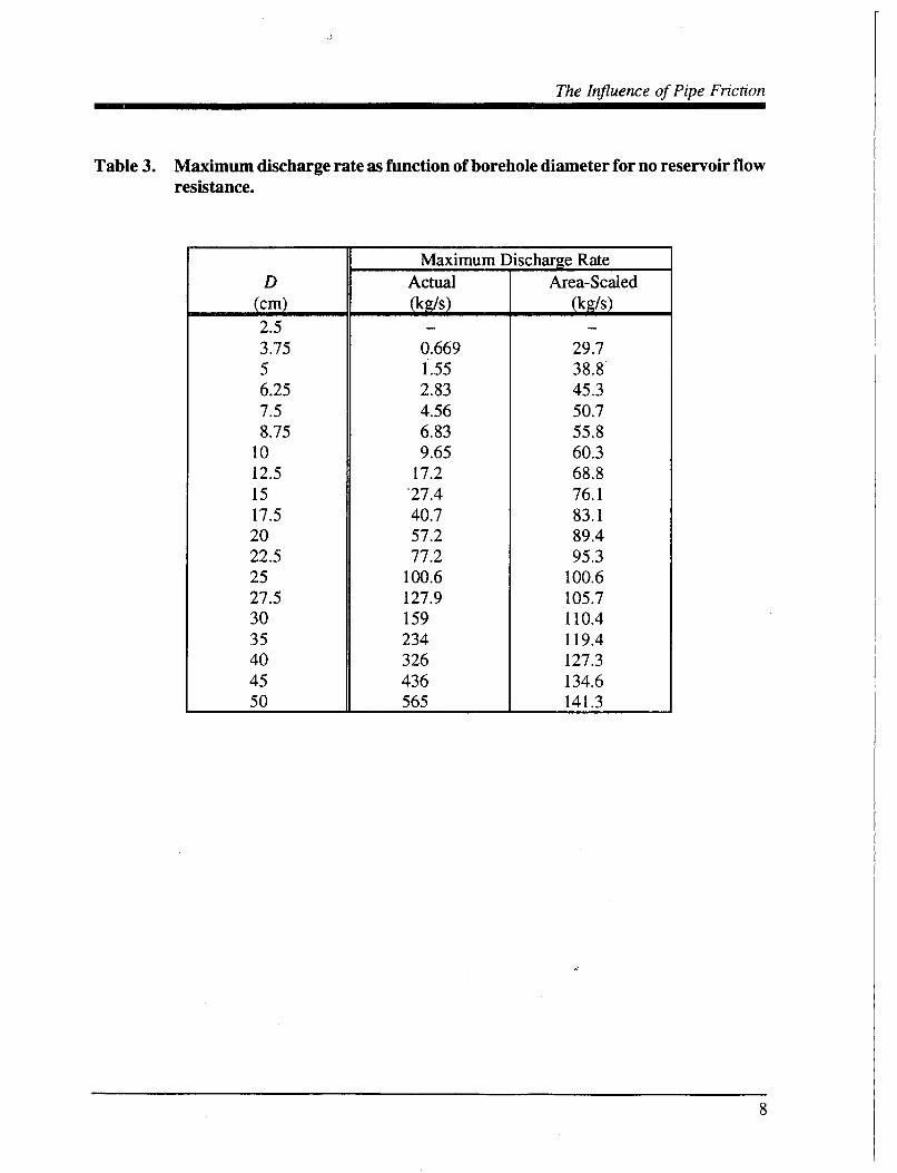
In other words, the frictional pressure gradient will be more important for the smaller-diameter core holes than for the largerdiameter well. Since the frictional pressm gmhent inmases with the squm of the discharge rate, this effect is most important at high flow rates. In Figure 2, we show how the maximum attainable flow rate depends upon borehole diameter for diameters between 2.5 cm (0.98 inch) and 50 cm (19.69 inches). Note that the borehole would not discharge at all for a diameter of 2.5 centimeters. Numerical values are provided in Table 3. The dotted line in Figure 2 is a straight line connecting the values for D = 10 cm and D = 25 cm. Essentially, the maximum flow rate (MmW) increases with borehole diameter (D) raised to the power -2.5. Therefore, the “area-scaled” maximum attainable flow rate (M*,& increases approximately with the square root of borehole diameter.
6

The Influence of Pipe Friction
1000
100
10
1
0. i 1 10
Well Diameter D (centimeters) 100
Figure 2. Maximum discharge rate (at one bar absolute wellhead pressure) as function of borehole diameter in the absence of reservoir flow resistance (bottomhole flowing pressure = 80 bars absolute).
7
The Influence of Pipe Friction 1
Table 3. Maximum discharge rate as function of borehole diameter for no reservoir flow resistance.
D (cm) 2.5 3.75 5 6.25 7.5 8.75
10 12.5 15 17.5 20 22.5 25 27.5 30 35 40 45 50
Maximum I Actual (kg/s) -
0.669
2.83 4.56 6.83 9.65
i s 5
17.2 '27.4 40.7 57.2 77.2
100.6 127.9 159 234 326 436 565
scharge Rate Area-Scaled
(kg/s)
29.7 38.8 45.3 50.7 55.8 60.3 68.8 76.1 83.1 89.4 95.3
100.6 105.7 110.4 119.4 127.3 134.6 141.3
-
d
8
4. THE INFLUENCE OF HEAT LOSSES
At relatively low flow rates, the effect of frictional pressure gradient is less important. We note, however, that the discharge performance curves shown in Figure 1 do not converge at low area- scaled flow rates either. For any value of the borehole diameter D, the discharge rate must lie between a particular maximum value and a particular minimum value for spontaneous flow to be possible. The variation of the minimum permissible flow rate with wellbore diameter is indicated in Figure 3; Table 4 contains numerid values. For small borehole diameters (less than 10 cm or so) the minimum permissible discharge rate is nearly independent of diameter and equal to about 0.5 kilogram per second. For larger pipe diameters, the minimum flow rate is greater, but the “area- scaled” minimum flow rate decreases monotonically with increasing borehole diameter.
This behavior is a consequence of the effects of heat losses fi-om the rising fluid within the wellbore to the formation outside. A typical situation within a flowing well under stable conditions as computed by the WELBOR program is illustrated in Figure 4. The well diameter is 25 centimeters (production-size well), and the discharge mte is 90 kilograms per second (near the maximum flow rate attainable from the well). Conditions are single-phase within the well from the feedpoint (at 1500 meters depth) up to about 980 meters depth. Above this point, two-phase flow takes place. Note that the temperature within the well is nearly constant below the boiling level, but that temperature increases with depth within the shallower two-phase region since temperatures and pressures in two- phase flow arc constrained to lie on the saturation curve for water. Also shown (as a dotted line) is the formation temperature profile assumed for these calculations. Note that the temperature inside the well exceeds that outside, particularly at shallow depths. Thus, it is to be expected that heat will be lost laterally from the fluid within the well to the cooler rock formations outside.
In Table 5, we show the decrease in specific enthalpy of the fluids discharged from the well relative to the initial bottomhole flowing enthalpy (1086.3 Joules per gram) for the same combinations of area-scaled discharge rates and borehole diameters considered in Table 2. Wellhead fluid enthalpies are lower than bottomhole enthalpies due to three effects: (1) increases in kinetic energy due to fluid expansion, (2) work done against gravity raising the fluid from the feedpoint level (1500 meteIis deep) to the wellhead, and (3) lated conductive heat losses to the formation. The work done against gravity is the same in all cases, and is equal to 14.7 Joules per gram. The effects of kinetic energy changes are even smaller, and reach maximum values for each borehole diameter at the maximum possible discharge rate; these maxima are, however, typically only a few Joules per gram. For flow rates significantly below the maximum value, kinetic energy changes amount to less than one Joule per &ram (see Table 6). Most of the energy changes listed in Table 5 are, therefore, due to lateral heat loss to the formation.
9

The Influence of Heat h s s e s
2 . 5
c5
'0 C 0 0 P)
L 0)
u) 2.0
a
L i
1 . 5 - .- Y
P) +., tl lx
Y
P) 1.0 z .c u v)
c3 .-
3 0.5 0- ....... @ ...... @ ..._ @...@@" E
C
x .-
0.0 1 10
Well 'Diameter D (centimeters) 100
Figure 3. Minimum discharge rate (at one bar absolute wellhead pressure) as function of borehole diameter in the absence of reservoir flow resistance (bottomhole flowing pressure = 80 bars absolute).
10 A

The Influence of Heat Losses
Minimum Actual (kg/s)
0.476 0.465 0.461 0.460 0.465 0.478 0.525 0.588 0.662 0.744 0.832 0.928 1.03 1 1.141 1.382 1.653 1.952 2.280
-
Table 4. Minimum discharge rate as function of borehole diameter for no reservoir flow
Discharge Rate Area-Scaled
(kg/s)
21.16 11.63 7.38 5.1 1 3.80 2.99 2.10 1.63 1.35 1.16 1.03 0.93 0.85 0.79 0.71 0.65 0.60 0.57
-
resistance.
I" 3.75 5 6.25 7.5 8.75
10 12.5 15 17.5 20 22.5 25 27.5 30 35 40 45 50
11

The Influence of Heat Losses
Steam Volume Fraction 0 20% 40% 60% 80% 100%
I I I I
- - - - - - - -
TEMPERATURE - - -
- .c -P -
- - - -
1250 - - Diameter = 25 'cm - Flowrate = 90 kg/s - -
I l l 1
0 SO 100 I SO 200 250 300 Degrees Celsius
0 20 40 60 80 100 120 B a r s (absolute)
Figure 4. Typical flowing conditions in production well. Note that reservoir flow resistance is assumed to be zero (bottomhole flowing pressure = 80 bars). Dotted line indicates formation temperature profile.
12

The Influence of Heat Losses
Table 5. Wellhead fluid enthalpy decrease (relative to Mtomhole flowing enthalpy) as a functim of borehie diameter (0) and area-scaled discharge rate (M*) neglecting flow resistance of reservoir (bottomhole pressure = 80 bars).
Area-Scaled Flow Rate
(kgN 10 20 30 40 50 60 70 80 90
100 110 120
Area-Scaled Flow Rate
(kg/s ) 10 20 30 ‘
40 50 60 70 80 90
100 110 120
Entries are specific enthalpy decrease, Jouleslgram Bc
7.5 43 1.2 258.2 182.7 139.3 109.9
-
- - - - - - -
ehole dim
10.0 280.3 160.6 113.8 88.8 72.4 63.1
-
- - - - - -
Zter (D), i
12.5 194.4 110.9 79.9 63.5 53.0 45.8
I
- - - - - -
Borehole diameter (D), i
3 20.0 89.2 53.8 41.1 34.4 30.4 27.6 25.6 24.4 - - - -
22.5 74.2 45.7 35.6 30.4 27.2 25 .O 23.4 22.4 22.3 -
- - I
25 .O 63.2 40.1 31.8 27.5 24.9 23.1 21.9 21 .o 20.6 23.6
27.5 55.0 35.7 28.9 25.4 23.2 21.6 20.6 19.9 19.5 19.9
I
- -
centimett
15.0 143.2 82.5 60.7 49.1 41.9 36.9 33.6
-
- - - - -
centimett
30.0 48.7 32.5 26.8 23.7 21.9 20.6 19.7 19:l 18.8 18.8 - -
b
17.5 110.9 65.1 48.8 40.3 34.9 31.3 28.8 27.8 - - - -
,
32.5 43.8 29.9 25 .O 22.4 20.8 19.7 19.0 18.4 18.2 18.1 19.0 -
20.0 89.20 53.8 41.1 34.4 30.4 27.6 25.6 24.4 - - - -
35.0 39.9 27.9 23.6 21.4 20.0 19.0 18.4 18.0 17.7 17.6 18.0
-
- Area-scaled flow rateM* = M x (25 cmlD)’. M is actual discharge rate.
13

The Influence of Heat Losses
Area Scaled Flow Rate
W s ) 10 20 30 40 50 60 60.3*
Table 6. Increase in fluid kinetic energy from bottomhole to wellhead as function of discharge rate for slim hole and production well.
Actual Hole Flow Rate ( k m 1.6 3.2 4.8 6.4 8.0 9.6 9.65*
Slim Hole) Specific Kinetic Energy Increase (Joules/gram)
0.0007 0.005 1 0.0169 0.0478 0.1614 3.5907 5.8237
Borehole Diameter = 25 cm (Production Well) Area Scaled Flow Rate
(kg/s) 10 20 30 40 50 60 70 80 90
100 100.6*
*Maximum well
Actual Well Flow Rate
(kg/s) 10 20 30 40 50 60 70 80 90
100 100.6*
ischarge rate
Specific Kinetic Energy Increase (Joules/gram)
0.0023 0.0082 0.01 86 0.0354 0.0620 0.1053 0.1812 0.3358 0.763 1 4.4146 6.0277
14

The Influence of Heat Losses
In the WELBOR k t losses to th treated by assuming XI Outward- directed heat flux from each element of the well surf.8ce given by
where TjUd is the local tempcratw of the fluid witkin the well, Trot- is the undisturbed rock fonmtion tempmtue distant from the boffhok at the sane dep&, and U is a heat transfer coefficient (i.e. Watts per square meter per dew Celsius). This heat transfer coefficient, in turn, may be approximated by:
( w k e D is borehole b m e w aabd II is the effective thmd conductivity of the rock formations ouiside the borehok-taken as 4 W I d C fix the present calcufations) as shown by Pritchett (198 1) bawd upon the work of h6dco-z aad cheng (196). la effsct, heat conduction takes place through a ''thermal boundary layer", with temperature qual to the borehole temperature at the inner edge of dwe boundary layer and equal to the reservoir temperature outside the boundary layer. Beyond the conductive boundary layer, heat transfer is dominated by convection in the porous reservoir rock. Minkowycz and Cheng (1 976) showed that the thickness of the boundary layer, at equilibrium, will be proportional to the borehole diameter. Based upon the above expression, it may easily be shown that the total power (i.e., Watts) lost by the fluid within the borehole is given by:
Total Power = 0 . 6 M Z dT (7)
where 2 is the depth of the borehole and dT is the vertically-averaged temperature difference between the borehole and the surrounding formation. Dividing the heat loss rate (from Eq. 7) by the rate of fluid production (M) yields the specific fluid enthalpy decrease due to heat losses:
For two boreholes of equal depths but of different diameters (01, D2), the ratio of the enthalpy change due to heat losses at the same area-scaled discharge rate (M*) will be:
In other words, heat losses will always be more significant for the slimmer of the two boreholes; the enthalpy loss will vary inversely with "ma-scaled" discharge rate and also inversely with the square of the borehole diameter. As shown in Table 5, the greatest enthalpy declines occur for relatively small-diameter boreholes openting at low discharge rates.
15
The Influence of Heat Losses
This difference in relative heat loss is responsible for the fact that “area-scaling” fails to produce the same discharge characteristics for production-size wells and for sl im holes, even at low flow rates. The computed wellhead pressure is shown in Figure 5 as a function of area-scaled flow rate (M*) for 10-cm s l im holes and for 25cm production wells both for the calculations described above (solid lines) and for a special series of calculations in which the heat-transfer coefficient was set to zero (dotted lines). Numerical values are provided in Table 7. The following are noteworthy: (1) for all flow rates, the wellhead pressure is larger if heat losses are neglected, (2) the difference in wellhead pressure between the “no-heat-loss,’ and “heat-loss” cases (for a ked borehole diameter) is greatest for the lowest discharge rates, (3) the influence of heat losses upon wellhead pressure is much greater for the 10-cm slim hole than for the 25-cm production well, and (4) in the absence of heat losses (compare the two dotted curves) the wellhead pressure becomes independent of borehole diameter and depends only on area-scaled discharge rate for low flow rates (where the effects of pipe friction are relatively unimportant).
The mechanism by which heat loss influences wellhead pressure may be understood by consideration of the flowing pressure distribution indicated by the green line in Figure 4. Note that, below the boiling interface, the vertical flowing pressure gradient is approximately hydrostatic (-80 bars per kilometer) but that within the two-phase zone above the boiling level the flowing pressure gradient is sigmficantly lower (-35 ban per kilometer in Figure 4). If heat losses increase, then the liquid temperature below the boiling surface will decline. As a result, the boiling level will occur at a shallower depth within the borehole, at the boiling-point pressure for the lower temperature. Therefore, a greater portion of the borehole will contain the high-pressure-gradient single-phase liquid region and a smaller portion will contain the low-pressure-gradient two-phase region. As a consequence, the average pressure gradient for the borehole as a whole will increase. Since the bottomhole flowing pressure is fixed, this means that the wellhead pressure must decline with increasing heat loss.
16
The Influerice of Heat 1~sse.c
3 1 1 01 01 (u
L 10 a
10 crn well - With neat loss
25 cm w e l l - no heat loss 25 cm well - w i t h heat loss 10 cm well - no heat loss
............
. . . . . . . . . , . .
0 20 40 60 80 100 Area-Scaled Well Total Discharge Rate ( k g / s )
Figure 5. Relative effects of heat losses to the formation on flowing characteristics of production wells (25 cm) and slim holes (10 cm).
17

The Influence of Heat Losses
Table 7. Influence of heat loss to formation on production well and slim hole performance.
Area Scalec Flow Rate M*
(kg/s) 1 2 3 4 5 7
10 15 20 25 30 35 40 45 50 55 60 65 70 75 80 85 90 95
1 00 105
Wellhead Pressure (bars)
Actual Flow Rate
M (kdd
0.16 0.32 0.48 0.64 0.80 1.12 1.6 2.4 3.2 4.0 4.8 5.6 6.4 7.2 8.0 8.8 9.6
10.4 11.2 12.0 12.8 13.6 14.4 15.2 16.0 16.8
No Heat Loss 4.30 7.09 8.40 9.22 9.80
10.58 1 1.26 11.81 11.96 11.87 11.57 11.07 10.37 9.41 8.1 1 6.24 2.68 - - - - - - - - -
I
With Heat Loss - - 1.02 2.17 3.3 1 5.24 7.20 8.98 9.85
10.23 10.28 10.06 9.58 8.82 7.70 6.02 2.85 - - - - - - - - -
Wellhead Pressure
Actual Flow Rate
M tkds)
1 2 3 4 5 7
10 15 20 25 30 35 40 45 50 55 60 65 70 75 80 85 90 95
100 . 105
2
No Heat Loss 4.72 7.41 8.70 9.5 1
10.09 10.88 11.62 12.31 12.69 12.89 12.98 12.98 12.9 1 12.76 12.56 12.29 11.95 11.53 11.04 10.45 9.74 8.89 7.84 6.45 4.29 -
With Heat Loss
1.37 4.96 6.84 8.02 8.85 9.94
10.93 11.83 12.32 12.60 12.74 12.78 12.73 12.61 12.43 12.17 11.85 11.45 10.97 10.39 9.70 8.85 7.81 6.44 4.29 -
I 18

5. THE DIFFICULTY OF INITIATING SLIM-HOLE DISCHARGE
b
Field experience has shown that it is frequently difficult (and sometimes impossible) to induce stable self-sustained discharge from slim deep holes (depth significantly greater than 300 meters) drilled into a field from which spontaneous discharge is readily obtained using wells of conventional diameter. While the greater importance of pipe friction in slim holes may play a limited role in this problem, the main reason appears to be the relatively larger heat losses to the surrounding formation for boreholes of small diameter.
As noted above, heat losses from the borehole to the formation under stable steady-flow conditions may be adequately represented using a heat transfer cokfficient of the form:
‘
U = 0 . 6 K / D
The problem is that the above formula is only applicable after a stable condition has been reached. The stable heat-transfer model discussed above involves a conductive boundary layer around the borehole of which the thickness is pmportional to the borehole diameter. Prior to discharge initiation, however (assuming that the borehole has previously been left in a shut-in condition for a long period of time)? the temperature distribution within the borehole will closely resemble that in the formation outside. When discharge begins, temperahms within the borehole change almost discontinuously to higher values. This induces the formation of a thermal boundary layer around the borehole of which the thickness increases with time, eventually reaching the asymptotic value described by Minkowycz and Cheng (1976). At early times, however, the boundary layer will be thinner than at steady-state, so that conductive heat transfer will be augmented. In short, the transient case may be regarded as a succession of states in which the heat transfer coefficient is a decreasing function of time which reaches the above asymptotic value only at infinite time. This situation may be described by defining a “heat loss multiplier” which declines toward unity as time goes on. Computed values for the heat transfer multiplier as a function of time after flow startup for various borehole diameters are illustrated in Figure 6.
Therefore, under transient conditions, the results computed above for the discharge capacities of boreholes of various diameters are overly optimistic since these calculations, by assuming steady heat transfer, underestimate the effects of heat losses at early times. To investigate this issue, a series of calculations was performed involving boreholes of both 10 cm and 25 cm diameters, with the “heat transfer coefficient” augmented by various factors relative to the stable steady value. Results are indicated in Figure 7, which shows the ranges of area-scaled discharge rates within which flow may occur as functions of this heat loss multiplier factor. The maximum flow rate is only weakly influenced by increases in heat loss (as expected in light of the above discussion), but the minimum possible discharge rate rises significantly with increases in heat loss. For each borehole diameter, the “critical” heat loss multiplier is reached when the borehole can no longer discharge at any rate.
19

Diflculty of Initiating Slim-Hole Discharge
1
0 . 0 1 0 . 1 1 10 100 1000 Time since S t a r t u p , hours
Figure 6. Effective heat transfer coefficient multiplier as a function of time after flow startup for various values of borehole diameter (centimeters).
20

1
I I 1 I I I I I I I I 1 1 1 1 1 I I I I I I I ~
10 100 H e a t L.oss Multipl ier
1000
Figure 7. Ranges of area-scaled discharge rate within which discharge is possiblc for 10-cm slim holes and 25-cni production wells, for various values of heat loss multiplier. Reservoir flow resistance neglected (flowing bottom hole prcssurc = 80 bars,).
21

Difficulty of Initiating Slim-Hole Discharge
This critical value is much larger (-148) for the 25cm production well than for the lOcm slim hole (critical multiplier value -16.2).
This difference in heat loss effects is probably responsible for the difficulty often encountered in inducing deep slim holes (depth >> 300 meters) to discharge. For example, if we assume that for stable discharge to occur the heat-loss multiplier must drop below one-fourth of the above “critical value”, as shown in Figure 8, it should be possible to sustain stable discharge in a 25cm production well after a transient period of about two minutes. To reach a comparable state for the 10-cm diameter slim hole qui res nearly one hour. Since transient processes associated with conventional flow-initiation techniques (swabbing, pressurization, gas injection etc.) usually involve time-scales of only a few minutes, this may explain why deep slim holes often fail to sustain discharge even after several initiation attempts when larger-diameter wells start flowing without difficulty. This implies that to induce deep slim holes to discharge, it may be necessary to employ unusual techniques such as pre-heating the borehole prior to startup.
22

Dijfkultv of' lriitiuting Slim-Hole Discliurge
1 I 1 1 1 1 1 1 ~ I I I I 1 1 1 1 I I I I I I l l I I I I 1 1 1 1 I I I I I IVrr - I
I 0 , O l 0 . I 1 10 100 1000
Time since S t a r t u p , hours
Figure 8. Time required for heat loss multiplier to drop to 1/4 of critical value for IO-cm diameter slim holes and 25-em diameter production wells.
23

6. INCORPORATION OF RESERVOIR FLOW RESISTANCE
Up to this point, all calculations presented have assumed that the resistance of the reservoir itself to fluid flow may be neglected compared to the resistance imposed by the borehole; in other words, all calculations have assumed a bottomhole flowing pressure of 80 bars absolute at the feedpoint (at a depth of 1500 meters in the borehole). For extremely permeable geothermal reservoirs, this may be an appropriate approximation. Under many realistic circumstances, however, the finite permeability of the reservoir causes the bottomhole flowing pressure to be appreciably less than the stable reservoir pressu~, and the amount of such pressure decline increases with increasing discharge rate.
In light of the purpose of this study, it is appropriate to ignore pressure-transient effects and to assume that the bottomhole flowing pressure may be related to the reservoir pressure and the discharge rate by a “productivity index’’ ( I ) so that:
(10) - Pbonomhole - Preservoir - ( I )
where M is the discharge rate and the productivity index ( I ) may be regarded as a constant for each borehole. For the remaining WELBOR calculations, this general form was assumed, and it was further assumed that the fluid flows isenthalpically from “reservoir” conditions (at P = PreseWoir = 80 bars, T = 250°C) to “bottomhole” conditions (at P = P ~ m ~ ~ e ) , then up the borehole.
The essential difficulty involved in performing ‘calculations with non-zero reservoir flow resistance (that is, values of the productivity index I which m less than infinity) is that of estimat- ing the proper value to use for I for various borehole diameters. It is frequently observed that, if several production wells (of about the same physical characteristics) are drilled into the same reservoir, they are found to be characterized by a wide variety of values of I . This is particularly true in hxtured reservoirs, in which the productivity index of a particular well depends mainly on the degree to which it happens to intersect productive fractures which are well-connected to the hcture network as a whole. For purposes of this study, the essential question is: if a “slim hole” is dnlled into a particular location, what is the relationship likely to be between the productivity index of the slim hole (Islim) and the productivity index that would have been obtained if instead a production- size well had been drilled (Iprod)? Obviously, it is not possible to provide a deterministic answer to this question which will be valid in all cases. It is, however, possible to make estimates of the probable ratios of brad to Islim which may be valid in a statistical sense, or at least to assign bounds to this ratio. For this purpose, it is useful to adopt the following mathematical form for the productivity index ratio of two boreholes of different diameters (Dslim, Dprod):
where the appropriate (presumably non-negative) value for the exponent p remains to be established.
24

7. ESTIMATION OF PRODUCTIVITY INDEX: CYLINDRICAL FLOW APPROXIMATION
As a first step, consider the classical “radial-flow” model for flow of fluid into a borehole. We assume that the reservoir consists of a homogeneous region of constant thickness (h) and of infinite lateral extent, bounded above and below by impermeable aquitards. The borehole penetrates completely through this permeable zone and produces fluid uniformly along the borehole surface. Under these. conditions, the steady flowing bottomhole pressure in the borehole may be written:
- 2 nkh ’bottomhole - c.eservoir
where k is the reservoir permeability, v is the reservoir fluid kinematic viscosity, rD is the “drainage radius” for the borehole and re is the “effective wellbore radius”. Typically, the “drainage radius” rD is very large, comparable to the average interwell spacing or the reservoir overall dimensions (i.e., hundreds or thousands of meters). The “effective wellbore radius” re may be related to the actual borehole diameter and the “skin factof (S) by:
re = (f) e-’
so that, for example, if the skin factor is zero the “effective wellbore radius” is equal to the actual borehole radius. For “damaged” boreholes (S > 0) re is less than the true borehole radius, whereas for “stimulated” boreholes re exceeds the actual borehole radius. The above formula permits the definition of the productivity index for the borehole:
2 nkh I = ln(rD/re)
Therefore, for two b reholes f different diameters (Dslim, Dprod) and the same skin factor (9, the ratio of the productivity indices for the boreholes will be given by:
In rD - In Dprod + S - 0.693 In rD - In DsIim + S - 0.693
Islim - Iprod
25

Estintrstion of Productivity Index: Cylindrical Flow Approximation
This means that the productivity index of the slim hole is likely to be somewhat less than that of the production well. In the limit of large values for the drainage radius, however, we obtain:
which means p + 0 (see Equation 1 I). considering the case (&,,, = 10 cm, Dpmd = 25 cm), values for the exponent p for various values of the drainage radius rD (from 100 meters to 10 km) and of the skin factor (from -5 to +5) are illustrated in Figure 9. Positive skin factors are much more commonly encountered in geothe!d wells than negative skin factors; thus, the cylindrical model suggests p values which are very s d c o m p d with uNty.
26

Estimation of Productivitv Index: Cvlindrical Flow Aunroximation
0
n
c, C a, C 0
X w 07 C
0 V
CI)
X c) U c
n
0
.^ -
I
0 n c,
> c,
.-
.-
9 U 0 L a
Dra i nage Rad i us
Figure 9. Productivity index scaling exponent (p) for various drainage radii ( r ~ ) and skin factor ( S ) values.
27

8. ESTIMATION OF PRODUCTIVITY INDEX: SPHERICAL FLOW APPROXIMATION
As an alternative, we note that geothermal reservoirs frequently consist of large thick volumes of fractured rock. Boreholes penetrating such a reservoir often do not produce from long open intervals, but instead appear to produce from one or more discrete “feedpoints” where the borehole intersects a thin permeable fracture zone. In pressure-transient test interpretation, it has therefore occasionally proved useful to abandon the traditional “line-source” radial-flow model (above) and instead to consider a “spherical-source” flow model. Here, we treat the reservoir as unbounded in all directions; the “feedpoint” is represented by a spherical void within h s reservoir, and fluid flows toward the spherical surface in all directions in a spherically symmetrical manner. The spherical void represents the highly permeable region of intersection of the borehole with the fracture. Under conditions of steady flow, the pressure at the surface of the spherical void will be given by:
where d is the diameter of the spherical void. Thus, the productivity index may be written:
so that the ratio of productivity indices will be given by:
The problem is then: what is the relationship between “spherical void diameter” (d) and borehole diameter (D)? One extreme case is obtained by assuming that d is directly proportional to D. This yields, for the productivity-index scaling exponent p :
p + 1 if d / D + constant
Another extreme argument is to assert that the “spherical void diametei’ is independent of borehole diameter and is, in effect, a property of the fracture network itself, so that:
p + 0 if d + constant
28

Estimation of Productivitv Index: Svherical Flow Avvroximution
The actual situation is likely to lie between the above two extremes. Tang (1988) studied the problem of limited-entry completions of boreholes in thick anisotropic porous reservoirs. Tang’s results may be expressed as follows, in terms of productivity index ratios:
1 ‘prod hprod In hslim - In( Dslim/2) + - In a
2
Here, Dprod and Dslim are the diameters of the production well and slim hole, respectively; a represents the anisotropy of the reservoir permeability distribution:
(where kH and kv are horizontal and vertical permeability respectively), and hprod and hslim represent the “feedzone thickness” for each borehole completion; the vertical thickness of the region over which fluid enters the borehole (usually just a few meters or so in fractured geothermal systems). Tang (1988) implicitly assumes that h >> D.
Adoption of Equation 20 means that we are now confronted with estimathg hslim and hprod. For simplicity, the following relationship is assumed for this purpose:
h=h,+bD (22)
where h, and b are constants. Note that if b = 0, then hsljm = hprod = h,; in this case the feedzone thickness is independent of hole diameter. Positive values forb indicate that larger-diameter holes will tend to have somewhat thicker feedzones.
In Figure 10, we show how the proper value of the productivity-index scaling exponent (p) depends upon h,, a and b according to Equation 20, taking DProd = 25 cm and Dslim = 10 cm. Val- ues are in the range 0 < p < 1 ; p decreases toward zero as feedzone thickness (h,) increases. Larger values of a (= kH/kv) tend to decrease p. Increasing b (=[h-h,]/D), on the other hand, tends to increase p . In the limit b + 00, p approaches unity. On the whole, values of p appear to be some- what larger in the case of the spherical flow model than for the cylindrical flow model (compare Figures 9 and 10).
29

1 i I I I I I I I I I I I I I 1 1 1
0
a
.P C a, C 0 a X w 1s) C
0
U v)
0 L a
0
0 1 m 10 m
Feedzone Thickness ho 100 m
Figure 10. I'raduclivily index scaling exponcnt (p ) iiiidcr various contlititrns I,;rsctl on results rcportcd by l'ang ( I 988).

9. RESULTS FOR FINITE RESERVOIR FLOW RESISTANCE
In light of the results from the above two analyses (for "radial" and "spherical" flow), it seems reasonable to assume that the productivity index for a slim hole will be related to that for the equivalent production-size well by the following:
where the exponent p takes on values between zero and unity. For any real situation, the proper value for p is likely to lie somewhere between these limiting values.
Therefore, a final series of calculations was performed involving three well configurations:
(1) a 25-cm diameter production well with productivity index Iprod,
(2) a 10-cm diameter slim hole using Isrim = ZPrd (that is, p = 0 scaling for productivity index), and
(3) a IO-cm diameter slim hole using ISlh = 0.4 x Iprd (p = 1 productivity index scaling).
Several values of Zprod were considered, as follows:
1 kg/second/bar (547 lbkourlpsi) 2 kg/second/bar ( 1094 lb/hour/psi) 3 kg/second/bar ( 1642 lb/hour/psi) 4 kg/second/bar (2 189 Ib/hour/psi) 6 kg/second/bar (3283 lb/hour/psi)
Computed results for wellhead pressure as a function of ma-scaled discharge rate m listed in Tables 8,9 and 10 (which also includes the corresponding results for the case of no reservoir flow resistance; infinite Z p d ) . Figures 1 1 a-1 1 f illustrate the results graphically-Figure 1 1 a compares the production well and slim hole discharge characteristics for the case of no reservoir flow resistance, and Figures 1 1b-1 If compare the various boreholes at successively smaller values of Ip& (increasing reservoir flow resistance).
It is notewofiy that changing the reservoir flow resistance has a greater influence upon the discharge characteristics of the production size (25 cm) well than upon those of the slim hole (10 cm). The reason is simply that the total resistance to flow is the sum of the effects of the reservoir
Continued on page 4 I
31

.... ............. ~ ......................
Results for Finite Reservoir Flow Resistance ~
Table 8. Performance characteristics of 25-cm diameter production well as a function of productivity index.
Area Scaled
Flowrate M*
( k d s ) 5
10 15 20 25 30 35 40 45 50 55 60 65 70 75 80 85 90 95
100 105
Actual Flowrate
M (kg/s)
5 10 15 20 25 30 35 40 45 50 55 60 65 70 75 80 85 90 95
100 105
Rowing Wellhead Pressure (absolute bars) for Production Well Productivity Index =
1 kg/s/bar
8.1 1 9.38 9.51 9.23 8.72 8 .OO 7.06 5.8 1 3.65 - - - - - - - - - - - -
2 kgls/bar
8.47 10.14 10.64 10.73 10.59 10.29 9.85 9.26 8.52 7.57 6.32 4.49 - - - - - - - - -
..
3 kg/s/bar
8.60 10.40. 11.03 1 1.25 1 1.25 11.09 10.80 10.40 9.87 9.21 8.38 7.32 5.90 3.60 - - - - - - -
4 kg/s/bar
8.66 10.53 11.23 11.51 1 1.58 11.49 11.29 10.97 10.55 10.02 9.35 8.52 7.46 6.06 3.82 - - - - - -
6 kCr/s/bar
8.72 10.66 11.43 11.78 11.91 11.90 11.78 11.55 11.24 10.82 10.30 9.65 8.86 7.87 6.58 4.67 - - - - -
infinity 8.85
10.93 11.83 12.32 12.60 12.74 12.78 12.73 12.61 12.43 12.17 11.85 11.45 10.97 10.39 9.70 8.85 7.81 6.44 4.29 -
1 32

Results for Finite Reservoir Flow Resistance
2
~~
Table 9. Performance characteristics of 10-cm diameter slim hole using p = 0 productivity index scaling rule.
3
Area Scaled
Flowrate M*
(kg/s) 5 10 15 20 25 30 35 40 45 50 55 60 65
7.17 8.89 9.60 9.97 9.91 9.55 8.89 7.86 6.30 3.59 - -
~~~~~
][Flowing Wellhead Pressure (absolute bars) for Slim Hole
7.18 8.92 9.74 10.06 10.03 9.72 9.12 8.19 6.79 4.5 1 - -
Actual Flowrate
M (kg/s)
0.8 1.6 2.4 3.2 4.0 4.8 5.6 6.4 7.2 8.0 8.8 9.6 10.4
Productiv
1 kg/s/bar
3.35 7.15 8.80 9.51 9.71 9.54 9.03 8.16 6.81 4.57 - - -
Index = . . . - 4
kg/s/bar 3.32 7.19 8.93 9.77 10.10 10.10 9.80 9.24 8.35 7.02 4.92 - -
6 kgls/bar
3.32 7.19 8.95 9.79 10.14 10.16 9.89 9.35 8.50 7.25 5.31 - -
infinity 3.31 7.20 8.98 9.85 10.23 10.28 10.06 9.58 8.82 7.70 6.02 2.85 -
33

Results .for Finite Reservoir Flow Resistance
Table 10. Performance characteristics of 10-cm diameter slim hole using p = 1 productivity index scaling rule.
Area Scaled
Flowrate M"
(kg/s) 5
10 15 20 25 30 35 40 45 50 55 60 65
Actual Flowrate M
(kg/s) 0.8 1.6 2.4 3 -2 4.0 4.8 5.6 6.4 7.2 8.0 8.8 9.6
10.4
Flowing Wellhead Pressure (absolute bars) for Slim Hole Productiv
1 kg/s/bar
3.40 7.08 8.52 9.00 8.91 8.37 7.36 5.67 1.91 - - - -
y Index =
2 kg/sibar
3.36 7.14 8.76 9.43 9.58 9.35 8.76 7.78 6.24 3.34 - - -
3 kg/s/bar
3.34 7.16 8.83 9.57 9.80 9.66 9.20 8.41 7.17 5.21 - - -
4 kg/s/bar
3.33 7.17 8.87 9.64 9.91 9.82 9.42 8.71 7.61 5.9 1 2.52 - -
6 kg/s/bar
3.33 7.18 8.90 9.71
10.02 9.97 9.64 9.00 8.02 6.55 4.05 - -
infinity 3.31 7.20 8.98 9.85
10.23 10.28 10.06 9.58 8.82 7.70 6.02 2.85 -

PRODUCTION WELL. PHODUCTlVlTY INDEX = INFINJTE
0 20 40 60 80 100 Area-Scaled Well Total Discharge Rate (kg/s)
Figure I 1 a. Wellhead pressure as function ofarca-scaled well dischargc rate for slirii Iiolc (10 cm diameter) arid production well (25 cni dianictcr) with no reservoir flow resistance.

PKOUUC'T I ON WE1.L. PRODUCT I V I TY I NDEX = 6 KG/SEC/BAi?
1) ' ' I ' ' ' ' " ' ' " ' ' I ' i ' ' ' ' ' ' ' ' ' ' I ' ' ' ' ' I ' " " ' "$ 25-crn production well 10-crn slim hole ( p = 0 ) 10-crn slim hole (p = 1 ) .. "......... , . .
0 20 40 60 80 100 Area-Scaled Well Total Discharge Rate ( k g / s )
Figure I Lh. Wellhead pressure as function of area-scalcd well discharge rate for slim hole (10 cm diameter) and production well (25 cni diameter) with production-well productivity index equal to 6 kilograms per second per bar.
36
PRODUCTION WELL PRODUCTIVITY INDEX = 4 K G / S E C / B A R
1
1
1
L a
0 20 40 60 80 10 Area-Scaled Well Total Discharge Rate (kg/s)
'0
Figure 3 IC. Wellhead pressure as function of area-scaled well dischargc rate for slim hole (10 cm diameter) and production well (25 cm diameter) with production-well productivity index equal to 4 kilograms per sccond per bar.

Kesul/.s lbr- Finite Resetvoir Flow Resistunw
1s
14
13
L 12 n
h
v)
U v
J 1 l l ~ l , , , l , l , , , , , , , I J I , , , I ( I , , I , , , I , , , , , I I , , , , , ,
- 25-cm production well - 10-cm slim hole ( p = 0 ) 10-cm slim h o l e (p = 1 )
I -
- -
- -
Figure 1 I d. Wellhead pressure as function of area-scaled well discharge rate for slim hole ( I O cm diameter) and production well (25 cm diameter) with production-well productivity index equal to 3 kilograms per second per bar.
-
-
-
-
-
-
-
-
-
2 -- -
1 t t l ~ ~ ~ " l " " " l ~ ' ~ l ~ ~ ~ ' ' ~ ~ ' ~ ~ ~ ~ ' ~ ' ' ~ ~ ' l ' ~ -
0 20 40 60 80 100
PRODUCTION WELL PRODUCTIVITY INDEX = 2 KG/SEC/Bhi?
15
14
13
Q, 1 1 5 ! 10 a, L a
U a, II
a 9
- 8
I .-
3
2
1 0 20 40 60 80 100
Area-Scaled Well Total Discharge Rate (kg/s)
Figure l l e . Wellhead pressure as function of area-scaled well dischargc rate for slim hole (10 cm diameter) and production well (25 cm diameter) with production-well productivity index equal to 2 kilograms per second per har.
39
Resulis ti)r Finite Reservoir. Flow Hesistutice
1s
' 4
13 c
ffl
U L 12 a I v
a, ' 1 L 3
l I / I , I J l , , ~ l J J , I , I l ~ I I I I , 1 1 1 1 ~ , I , I , I I I , ~ I J I I , I I ~ I
- 2s-cm production well - - I 10-cm slim hole (p = 0 )
. . . . . . . . . . . . . . IO-cm slim hole ( p = 1 ) - -
-- -
: -
17igiir-e 1 I f. Wcllhcad pressure as function of area-scaled well discharge rate for slim hole (IC) cm dianieter) and production well (25 cm diameter) with production-well prodiictivity index equal to 1 kilogram pcr second per bar.
PRODUCT I ON WELL PRODUCT' I VI T'Y I NDEX = 1 KG/SEC/BAII
-
-
-
-
-
-
-
3 - -
-
2 -. -
I ~ ~ ~ ~ " " " " " " " " l l " " l ' ~ ' l " " ' ' i ~ ' ' ~ ' ~ " ~ ' ' ~ ' 0 20 40 60 80 100
40
Results for Finite Reservoir Flow Resistance
and of the borehole itself. As discussed above (see Elgure 2). the capacity of the borehole to deliver fluid to the wellhead varies approximately as 02.5, whereas the capacity of the reservoir to deliver fluid to the feedpoint varies as D, with 0 e p c 1. Consequently, the reservoir resistance comprises a greater proportion of the total resistance for larger diameter holes, and therefore large holes are more sensitive to variations in reservoir flow resistance.
It is also noteworthy that, despite the shortcomings of “area-scaling” of discharge rates (arising from the failure of the effects of pipe friction and of heat losses to scale in this manner), scaling-up the discharge characteristics of the 10-cm slim hole provides a conservative estimate of the probable productivity of larger diameter wells so long as the reservoir flow resistance is not too large (productivity index > 1 kg/second/bar or so), at least for conditions similar to those considered in this study.
41

IO. CONCLUSIONS AND RECOMMENDATIONS
The preceding computational study provides a theoretical framework within which the question of relative discharge chaxacteristics of slim holes and production wells may be examined. A number of issues require resolution by examination of field measurements and historical experience with slim holes in real geothermal fields, however.
One of these issues is the question of the “scaling rule” for downhole productivity index between slim holes and wells of conventional diameter. In this study, the following form was adopted:
and various arguments were advanced suggesting that the proper value for the exponent p should lie somewhere between zero and unity. It would be highly desirable to establish an appropriate empirical value for p based on field experience. One approach would be to examine one or more data sets from geothermal fields in which a sufficient number of both slim holes and production wells have been drilled and tested to provide a statistically significant sample. If sufficient productivity- index determinations are not available, the same p exponent should in principle govern the ratios of “injectivity indices” so that injection-test data, if available, could be substituted.
The calculations presented in Section 9 indicate that, if slim test holes can be induced to discharge, the fluid discharge capacity of the slim holes may be scaled up to equivalent production well capacities using the “area-scaling” rule (that is, by multiplying the observed slim-hole discharge rates by the square of the ratio of the wellbore diameters), and that this will usually provide a conservative forecast (i.e., underestimate) of production well performance so long as the reservoir permeability is monably good. The difficulty is that it may be very difficult to induce spontaneous discharge in deep slim holes (depth >> 300 meters) even in reservoirs with promising chamcteristics, for the reasons discussed in Section 5. Field experience with attempts to discharge slim holes (and comparisons with experience discharging production-size wells in the same field) should be examined to elucidate these issues and to suggest practical remedies if difficulties are encountered. The possibility of “,-heating” the slim hole prior to discharge initiation should be considered, and any available field experience with such techniques should be carefully studied.
If it is impractical to discharge the slim exploration holes, another possibility is to perform an injection test (with a downhole pressure gauge located near the feedpoint) and thereby to obtain an empirical “injectivity index” for the borehole. At least three types of difficulties are inherent in
42

Conclusions and Recommendations
this approach, however. First, it is much more important for an injection test than for a production test that the pressure gauge be located adjacent to the borehole feedpoint owing to hydrostatic differences arising from the temperature contrast between the cold injected fluid (of which the downhole temperature is likely to change sigdicantly with time during the test) and the hot reservoir waters. This means that it will be necessary to accurately identify the borehole’s feedpoint (by, for example, spinner logging) prior to injection testing. If, as is often the case, the borehole has more than one major feedzone, the interpretation of injection test results may be impossible. Second, it is very important that as much debris as possible (chips, etc.) be removed from the borehole prior to injection testing. Otherwise, this debris will tend to be carried into the feedzone of the borehole during the injection test, blocking important flow channels and rendering any test interpretation ambiguous. The third difficulty with the “injection test” approach is that an injection test raises fluid pressures in the neighborhood of the borehole. These increased fluid pressures will often open and/ or widen existing fiactum, increasing the local permeability and temporarily decreasing the reservoir flow resistance compared to what would occur under production (pressure reduction) conditions. This can result in overly optimistic estimates of borehole productivity under discharge conditions. Clearly, if injection testing is employed, it would be very desirable to carry out the test at relatively low injection rates to avoid excessive pressure increase. Any existing field experience concerning the relationships between observed “productivity index” and “injectivity index” for individual boreholes as functions of flowme, pressure and borehole diameter would undoubtedly prove useful in the interpretation of future injection tests.
43

11. REFERENCES
Dukler, A. E., M. Wicks 111 and R. G. Cleveland (1964), ‘‘Frictional Pressure Drop in Two-Phase Flow-B. An Approach Through Similarity Analysis”, A. I. Ch. E. J., v. IO, p. 44.
Hughmark, G. A. (1962), “Holdup in Gas-Liquid Flow”, Chem. Eng. Progr., v. 53, p. 62.
Minkowycz, W. J. and P. Cheng (1976), “Free Convection about a Circular Cylinder Embedded in a Porous Medium”, Int. J. Heat and Mass T r w e r , v. 19, p. 805.
Pritchett, J. W. (1981), “The LIGHTS Code”, S-Cubed Report Number SSS-R-80-4195-R1.
Pritchett, J. W. (1983, “WELBOR: A Computer Program for Calculating Flow in a Producing Geothermal Well”, S-Cubed Report Number SSS-R-85-7283.
Tang, R. W. (1988)’ “A Model of Limited-Entry Completion Undergoing Spherical Flow”, SPE Formation Evaluation, December, p. 76 1.
1
44

~ ~ ~~ ~ ~~~ ~~ ~~ ~
APPENDIX A. MATHEMATICAL FORMULATION OF TWO-PHASE FLUID FLOW IN A WELLBORE
Two-phase fluid flow in the wellbore is, at present, not amenable to strict analytical treatment. Depending upon the relative amounts of gas and liquid, a variety of flow patterns can occur in the pipe. At small gas loadings, bubble flow takes place. An increase in gas flow rate can result in slug, churn, or annular flow. Existing techniques for treating two-phase flow in the pipe require use of empirical correlations for flowing gas quality and friction factor (see below). There exist in the literature numerous such correlations; most of these correlations are based on flow in two-phase petroleum (oil and gas) wells. Utilization of different empirical correlations often yields widely different results; at present, there does not appear to be sufficient basis for selecting one or another of these correlations.
Consider two-phase non-isothermal steady flow in a vertical or deviated pipe. The bottom of the pipe is taken to be above the location of the topmost feedzone. The assumption of steady flow implies that the mass flux &f is constant along the length of the pipe:
&f = A{ Slplvl + Sgpgvg) = Apv = constant (1)
where
A = cross - section area of pipe p l ( p g ) = liquid (gas) density
vl ( vg ) = liquid (gas) velocity S,(Sg) = liquid (gas) volume fraction
z = vertical coordinate (positive upwards) p = mixture (liquid + gas) density = S p l + Sgpg
v = mixture (liquid + gas) velocity = (Slpfvf + Sgpgvg) /p
The pressure drop due to fluid flowing in a vertical or inclined pipe represents the combined effects of friction, acceleration, and change in elevation.
A- 1
Mathematical Formulation of Two-Phase Fluid Flow in a Wellbore
where
F = frictional pressure gradient g = g(z) , component of acceleration of gravity parallel to the well.
The frictional pressure gradient F is specified by empirical correlations. The S-Cubed wellbore simulator (WELBOR) uses Dukler’s correlation (Dukler, et al., 1964).
The mixture energy balance for two-phase flow can be expressed as follows:
where
eg = hg + v l / 2 = Eg +-+vg2/2 P p g
el = hl +v:/2 = El +--+$I2 P Pl
hg ( hl ) = gas (liquid) specific enthalpy
Eg ( El ) = gas (liquid) specific internal energy
upward gas mass flow rate ASgp,vg - - Qfg = flowing quality = total mass flow rate ni
rw = pipe radius T = fluid temperature
TR = formation temperature, U = heat transfer coefficient
The last term in Equation (3) describes the heat loss from the borehole to the surrounding formation. If the formation outside the wellbore is impermeable, then the heat flux from the borehole will decline with time (lim U = 0) as the rock near the borehole heats up. Generally, the formation outside the wellbo&% permeable, and the heat loss will occur due to combined effects of conduction and convection. Analytical results of Minkowycz and Cheng (1976) suggest that the heat transfer coefficient in the latter case is given by:
lim U = 0.3K/rw t+-
(4)
A-2

Mathematical Formulation a f Two-Phase Fluid Flow in a Wellbore
where K is the thermal conductivity of the water saturated formation. With typical values of K (= 4 W/m-"C) and r,,, (= 0.1 m), the heat transfer coefficient equals 12 W/m2-"C. In practical applications, U generally lies between 5 and 20 W/m2-"C.
The momentum balance law constitutes a single equation for two unknowns, i.e., liquid and gas velocities vI and vg. To solve for vl and vg, we need another relation between vl and vg. For this purpose, it is convenient to express vI and vg in terms of flowing quality Qfg.
where Q, denotes the in situ gas quality. We shall now consider the specification of Qfg in terms of other known flow properties. The simplest assumption is to take flowing quality Qfg equal to the in situ quality Q,. This is the so-called no-slip approximation (VI = us). In practice, the no-slip approximation predicts too low a pressure drop in the wellbore. In general, one would expect the gas phase to rise more rapidly in the wellbore than the liquid phase due to buoyancy. If us 2 V I , then it follows from Equation ( 5 ) that the flowing quality Q is also
numerous empirical cQrrelations in the literature which can be used to express Qfg in terms of Qs and other flow properties. The S-Cubed wellbore simulator (WELBOR) incorporates a correlation due to Hughmark (1962). Hughmark's correlation is in part based on liquid water and steam flow through vertical and horizontal tubes. Experience has shown that the use of Hughmark's correlation often yields too high a value for the pressure drop. To obviate the difficulties associated with the original Hughmark correlation, S-Cubed' s WELBOR simulator uses a modified version of the Hughmark correlation; essentially, the slippage rate may vary between the value given by the Hughmark correlation and no-slip at all, according to the value of a user supplied parameter (slip parameter). This feature is normally used only for fitting measured downhole pressure and temperature profiles; in normal operations, the program simply uses the original Hughmark correlation. Typical slip parameter values required to fit downhole data from particular boreholes vary between 0.5 x Hughmark and 1 .O x Hughmark.
greater than or at least equal to the in situ quality Q,. As already mentioned above, t I? ere exist
The mass, momentum, and energy balance laws need to be adjoined by a suitable equation-of-state for the fluid. With pressurep and mixture enthalpy h (or alternatively mixture energy E ) as independent parameters, the equation-of-state routines can be used to calculate dependent variables such as Eg, El, pl, pg, T, Qs, Sg, SI, pl and pg.
A-3
Mathematical Formulation of Two-Phase Fluid Flow in a Wellbore
The capacity of a borehole to deliver fluid to the wellhead is limited. The so-called “choking condition” occurs when dp ldz becomes singular. The maximum flow capacity of a borehole is obviously somewhat less than that for whch choking first occurs. For two-phase flow with slip, the choking condition is given by:
For the no-slip case (vg = vl), the above choking condition reduces to the following familiar form:
I = v2/c2
where c(= [l/(ap/a~)~]~’~) denotes the speed of sound.
(7)
A-4

DISTRIBUTION
David N. Anderson Geothermal Resources Council PO Box 1 3 5 0 Davis, CA 9 5 6 1 7
Jim Combs Geo Hills Associates 2 7 7 9 0 Edgerton Road Los Altos Hills, CA 9 4 0 2 2
Greg Taylor Christensen Boyles Corporation PO Box 3 0 7 7 7 Salt Lake City, UT 8 4 1 3 0
Alan Melchior Far West Capital 9 2 1 Executive Park Drive, Suite B Salt Lake City, UT 84117
Colin Goranson 1 4 9 8 Aqua Vista Road Richmond, CA 9 4 8 0 5
Jim Lovekin California Energy Co. 9 0 0 North Heritage, Bldg D Ridgecrest, CA 9 3 5 5 5
Marc Steffen Cal-Pine Corporation 1 1 6 0 North Dutton, Suite 2 0 0 Santa Rosa, CA 9 5 4 0 1
Walter Haenggi Magma Power Company 5 5 1 West Main Street, Suite 1 Brawley, CA 9 2 2 2 7
Bureau of Land Management ( 2 ) Attn: Michael Ferguson
7 8 7 N. Main, Suite P Bishop, CA 9 3 5 1 4
Cheryl Seath
Robert Deputy ARC0 Oil and Gas Co. 2 3 0 0 W. Plano Parkway Plano, TX 7 5 0 7 5
Sue Goff
Los Alamos, NM 8 7 5 4 5 LANL, MS D - 4 4 3
Charles George Hall ibur ton Services Drawer 1 4 3 1 Duncan, OK 7 3 5 3 6
Barry Harding Ocean Drilling Program Texas A&M University 1000 Discovery Drive College Station, TX 7 7 8 4 0
George Cooper Dept. of Materials Science & Mineral Engineering
University of California Berkeley, CA 9 4 7 2 0
Helene Knowlton Smith International 1 6 7 4 0 Hardy Street Houston, TX 7 7 2 0 5
Frank Monaster0 US Navy - Geothermal Office China Lake, CA 9 3 5 5 5
John Mastor Longyear Company PO Box 1000 Dayton, NV 8 9 4 0 3
B. J. Livesay 1 2 6 Countrywood Lane Encinitas CA 9 2 0 2 4
Daniel Lys ter Mono County Energy Mgmt HCR 7 9 , PO Box 2 2 1 Mammoth Lakes, CA 9 3 5 4 6
Desert Drilling Fluids ( 4 ) Attn: Gene Polk
3316 Girard Blvd NE Albuquerque NM 87107
Dave Donald
Nic Nickels Eastman Christensen 3 6 3 6 Airway Drive Santa Rosa, CA 9 5 4 0 3
Steve Pye Unocal Geothermal PO Box 7 6 0 0 Los Angeles, CA 9 0 0 1 7

John Sass USGS 2255 North Gemini Drive Flagstaff, AZ 86001
Larry Larson Nabors Loffland 515 West Greens Road, Suite 310 Houston, TX 77067
Tonto Drilling Services (2) Attn: George McLaren
Larry Pisto PO Box 25128 Salt Lake City, UT 84125
Tommy Warren Amoco Production Center PO Box 3385 Tulsa, OK 74102
G. S. Bodvarsson Earth Sciences Division Lawrence Berkeley Lab 1 Cyclotron Road Berkeley, CA 94720
US Department of Energy (3) Geothermal Division Attn: Ted Mock
Lew Pratsch Marshall Reed
Forrestal Bldg., CE-324 1000 Independence Ave. SW Washington, DC 20585
Susan Hodgeson Division of Oil and Gas 20th Floor, MS-20 801 K Street Sacramento, CA 95814-3530
Elizabeth Johnson Div. of Oil and Gas - Geothermal 20th Floor, MS-21 801 K Street Sacramento, CA 95814-3530
Warren Bollmeier PICHTR 2800 Woodlawn Dr, Suite 180 Honolulu, HI 96822
Dick Benoit Oxbow Power Services, Inc 200 South Virginia St, Suite 450 Reno, NV 89501
George Darr Geothermal Program Manager Bonneville Power Administration PO Box 3621 Portland, OR 97208-3621
Mohinder Gulati UNOCAL Geothermal PO Box 7600, Room M-36 Los Angeles, CA 90051
Thomas C. Hinrichs Magma Power Company 11770 Bernard0 Plaza Ct, Suite 366 San Diego, CA 92128
Tsvi Meidav Trans-Pacific Geothermal Corp. 1901 Harrison St, Suite 1590 Oakland, CA 94612
Joel Renner Manager, Renewable Energy Programs Idaho Nat'l Engineering Lab. PO Box 1625 Idaho Falls, ID 83415
Richard Thomas Geothermal Officer Calif. Div of Oil & Gas 1416 Ninth St, Room 1310 Sacramento, CA 95814
7141 Technical Library (5) 7613-2 For Document Processing
for DOE/OSTI (10) 7151 Technical 'Publication (2) 6000 D. L. Hartley 6100 R. W. Lynch 6111 J. C. Dunn (10) 6111 J. T. Finger (20) 6111 R. D. Jacobson 6111 D. A. Glowka 6111 P. C. Lysne 6111 R. D. Meyer 6111 D. M. Schafer 6114 R. S. Harding 4112 K. G. Pierce 1511 C. E. Hickox, Jr 1513 R. R. Eaton 8523-2 Central Technical Files


![arXiv:1103.3518v3 [astro-ph.SR] 18 Aug 2011 and Astrophysics inPune, India. The fielddecay ch aracteristics of both configurations isinvestigated and compared with previous calculations](https://img.dokumen.tips/doc/110x75/5b39125a7f8b9a1a678c24ff/arxiv11033518v3-astro-phsr-18-aug-2011-and-astrophysics-inpune-india-the.jpg)


![Chapter 1 An In tro duction to Mathematic a - USNA · Chapter 1 An In tro duction to Mathematic a 1.1 In tro duction ... form ulas for ro ots of ... -1 == 0,x] Mathematic a nds all](https://img.dokumen.tips/doc/110x75/5b502a917f8b9a346e8de305/chapter-1-an-in-tro-duction-to-mathematic-a-chapter-1-an-in-tro-duction-to.jpg)


