Elements of Linear Algebra: Q&A - Home | University of ... · Elements of Linear Algebra: Q&A A matrix is a rectangular array of objects (elements that are numbers, functions,

75

Elements of Linear Algebra: Q&AA matrix is a rectangular array of objects (elements that are

numbers, functions, etc.) with its size indicated by the number of rows and columns, i.e., an m×n matrix A with m rows and ncolumns.

If A is an m×n matrix, AT is an n×m matrix.The determinant of a matrix is the absolute value of the sum of the

diagonal elements. The determinant is only defined for a square matrix. The determinant of a matrix can be computed using the Laplace expansion where a row or column is expanded in terms of minors and cofactors.

An orthogonal matrix is an invertible n×n matrix Q with the property Q−1 = QT.

76

Elements of Linear Algebra: Q&AGiven a system of m linear equations in n variables xi (i = 1, …, n),

written as Ax = b, the system is either1. Consistent, with a unique (one) solution x.2. Consistent, with infinitely many possible solutions.3. Inconsistent with no solutions.

If n > m, the system has more unknowns than equations it is underdetermined. If the system is consistent, some of the variables can be chosen arbitrarily and the remaining variables defined in terms of the arbitrary ones.

If n < m, the system has more equations than unknowns it is overdetermined.

77

Elements of Linear Algebra: Q&AP3.16. Invertible matrix properties Assume that A is an n × n

invertible matrix. Which statements are true?a. The system Ax = b has a unique solution for every vector b

in Rn.b. The rows (and columns) of A are linearly independent.c. det(A) = 0.d. A can be reduced (by elementary operations) to the identity

matrix.e. The rank of A is n.f. The rows of A span Rn.

78

Elements of Linear Algebra: Q&A

2 2

2 2 2

4 2 2 2

4 2 2

1CO + O = CO .21H + O = H O.2

CH + 2O = CO + 2 H O.3CH + O = CO + 2 H O.2

P3.18. Linear Independence Consider the equations of combustion in which a mixture of CO, H2, and CH4 are burned with O2 to form CO, CO2 and H2O.

Treating the compounds as real variables, determine if the equations are independent. If not, write the dependent equation(s) in terms of the independent ones.

79

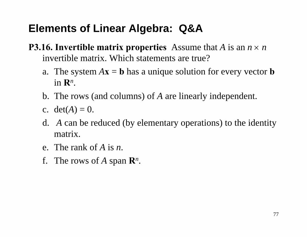
Elements of Linear Algebra: AEM P2.35

80

Elements of Linear Algebra: AEM P2.35

81

Eigenvalues & EigenvectorsAs an engineer, you have undoubtedly been introduced to eigenvalues and possibly eigenvectors. We develop background here and will later make use of eigenvalues/vectors in the discussion of second and higher-order tensors. Given the linear equation the vector x is called the eigenvector (characteristic vector) and the scalar λ is the eigenvalue (characteristic value) of matrix A that characterizes the length (and sense) of the eigenvector x. The spectrum of A is the set of eigenvalues of A and the spectral radius of A is the absolute value of the largest eigenvalue.

Elements of Linear Algebra

A =x b

82

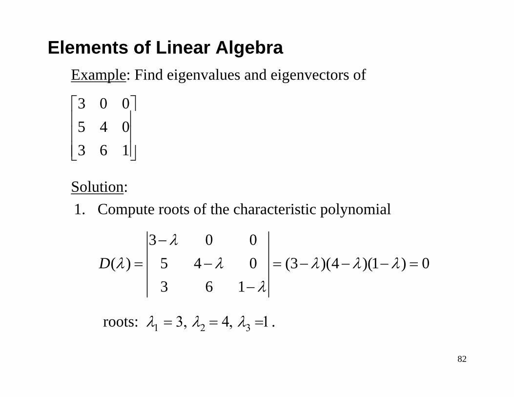
Example: Find eigenvalues and eigenvectors of

Solution:1. Compute roots of the characteristic polynomial

roots: λ1 = 3, λ2 = 4, λ3 =1.


3 0 05 4 03 6 1

⎡ ⎤⎢ ⎥⎢ ⎥⎢ ⎥⎣ ⎦

3 0 0( ) 5 4 0 (3 )(4 )(1 ) 0

3 6 1D

λλ λ λ λ λ

λ

−= − = − − − =

−

83

These roots are the eigenvalues. They form the spectrum with a spectral radius of 4.

2. Compute the eigenvectors:λ1 = 3

λ2 = 4


1 2 1

1 2 3

0 0 1 25 0 set 1 5 or 10

27 / 2 273 6 2 0x x x

x x x

= − −⎫ ⎡ ⎤ ⎡ ⎤⎪ ⎢ ⎥ ⎢ ⎥+ = → = → = − −⎬ ⎢ ⎥ ⎢ ⎥⎪ − −⎢ ⎥ ⎢ ⎥+ − = ⎣ ⎦ ⎣ ⎦⎭

x

1

1 2

1 2 3

0 05 0 set 1 1

23 6 3 0

xx x

x x x

− = ⎫ ⎡ ⎤⎪ ⎢ ⎥= → = → =⎬ ⎢ ⎥⎪ ⎢ ⎥+ − = ⎣ ⎦⎭

x

84

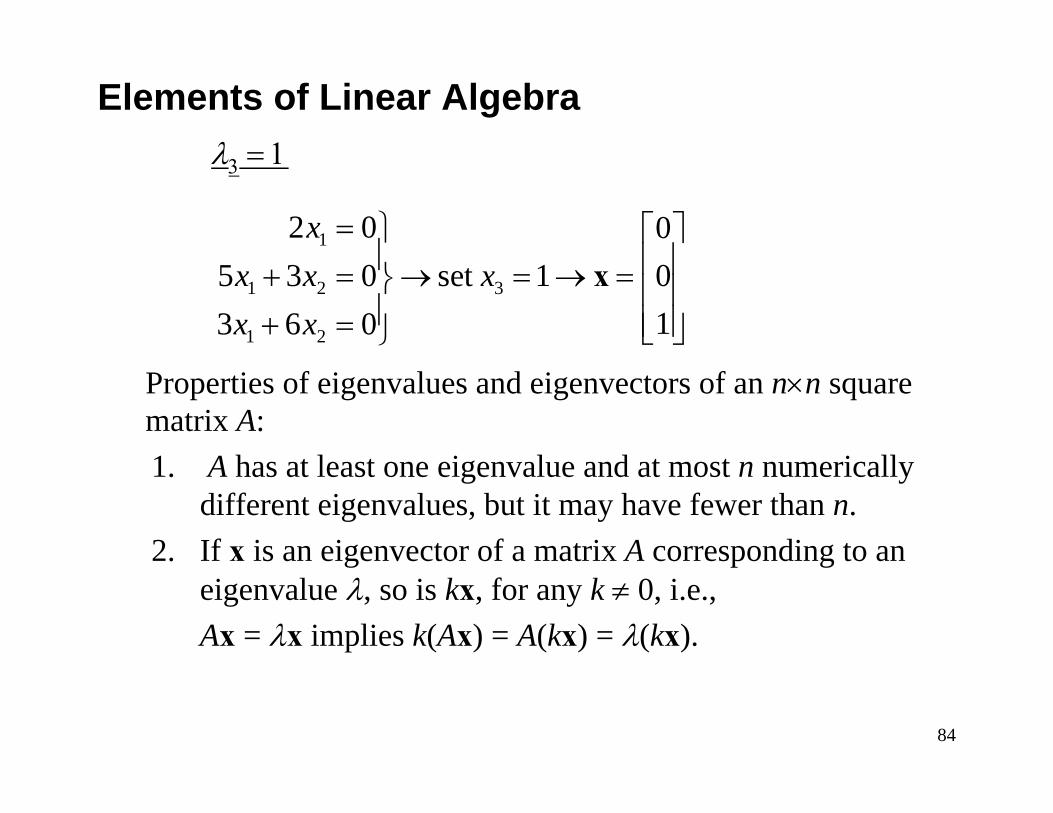
λ3 = 1

Properties of eigenvalues and eigenvectors of an n×n square matrix A: 1. A has at least one eigenvalue and at most n numerically

different eigenvalues, but it may have fewer than n. 2. If x is an eigenvector of a matrix A corresponding to an

eigenvalue λ, so is kx, for any k ≠ 0, i.e., Ax = λx implies k(Ax) = A(kx) = λ(kx).


1

1 2 3

1 2

2 0 05 3 0 set 1 0

13 6 0

xx x xx x

= ⎫ ⎡ ⎤⎪ ⎢ ⎥+ = → = → =⎬ ⎢ ⎥⎪ ⎢ ⎥+ = ⎣ ⎦⎭

x

85

3. Mλ is the algebraic multiplicity, the number of times the root λ of the characteristic polynomial is repeated, and mλis the geometric multiplicity, the number of independent eigenvectors corresponding to λ. According to property 1 above, the sum of algebraic multiplicities equals n and in general mλ ≤ Mλ.

4. A real matrix may have complex eigenvalues that occur in conjugate pairs and complex eigenvectors.

5. The eigenvalues of a symmetric matrix (AT = A) are real. 6. The eigenvalues of a skew symmetric matrix (AT = −A) are

pure imaginary or zero.


86

Eigenvectors & DiagonalizationSimilar matrices have the same spectrum (i.e., same eigenvalues),

n×n matrix , is similar to A for some n×nmatrix T.

This is an important property, particularly for numerical analysis, to diagonalize (or nearly diagonalize) matrices for computing approximations to eigenvalues and eigenvectors.The eigenvectors corresponding to a set of distinct eigenvaluesform a linearly independent set. Thus, these eigenvectors form a basis. If an n×n matrix A has a basis of eigenvectors, then is diagonal with eigenvalues of A as the entries on the main diagonal.


1ˆ :A T AT−=

1D X AX−=

A

87

The vector algebra included operations involving sums and products of vectors. The definitions and operations defined in the linear algebra provide the basis for linear transformations and matrix operations useful in tensor analysis.The vector calculus allows us to apply the methods of differential and integral calculus in the general tensor analysis. We begin with the usual basic definitions and operations. Derivative of a Vector Function of a Scalar

Vector Calculus & General Coordinate Systems

a(t + ∆t)

a(t)

∆as

ˆ se0

0

( ) ( )lim

| |

ˆlim

t

st

d t t tdt ts

d s dsdt s t dt

∆ →

∆ →

+ ∆ −=

∆∆ =

∆ ∆= =

∆ ∆

a a a

aa a e

88

Product Rules

Note that because a vector is composed of two distinct parts, magnitude and direction, a nonzero derivative could result from: a) a change in magnitude but not direction, b) a change in direction but not magnitude, or c) a change in both magnitude and direction as illustrated in the previous diagram.


( )

( ) (order preserved)

d d ddt dt dtd d ddt dt dt

⋅ = ⋅ + ⋅

× = × + ×

a ba b b a

a ba b b a

89

For case b), a constant length vector,

In general coordinates, the base vectors are not necessarily constant in magnitude or direction,

By definition, the base vectors of Cartesian systems have constant magnitude and direction


2

| | const

const| |

( ) 0| | const

const| |

ddt

d d daa adt dt dt

ddt

⎧ =⎧⎪⎪ = ⎨⎪ =⎪⎪ ⎩⋅ = → ⋅ = ⋅ = ⎨

=⎧⎪ ⎪⎪ ⊥ ⎨ ≠⎪ ⎪⎩⎩

aa 0 a

aaa a aa

aa aa

ii i i

i iddaa a

dt dt= → +

ea e e

/ .id dt→ =e 0

90


Example: Compute the acceleration of a body in a circular orbit.

r(t)r(t + ∆t)

v(t + ∆t)v(t)

v(t)

v(t + ∆t)

∆v

ˆˆ

ˆ

z

r

t

rv

ω=== × =

ω er ev ω r e

91


2

2

2

( )

ˆ

ˆ ˆ ˆ ˆ( ) [ ( )]

ˆ ˆ ˆ ˆ ˆ ˆ[( ) ( ) )]

ˆ

z

z z z r

z r z z z r

r

d d d ddt dt dt dtv dr dtv vr rvrvr

= = × = × + ×

= × + × = ×

= × × = × ×

= ⋅ − ⋅

= ⇐

v ω ra ω r r ω

e r ω v ω v

e ω r e e e

e e e e e e

e

92

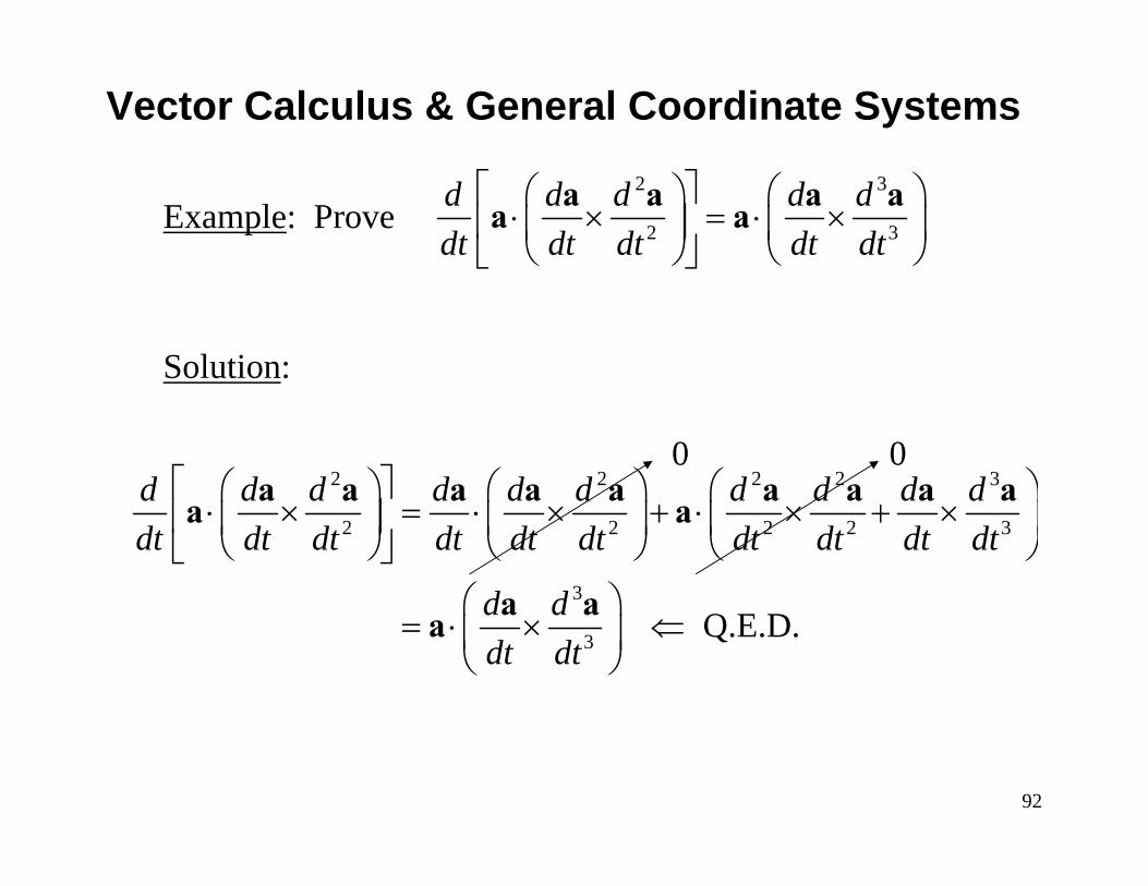
Example: Prove

Solution:


2 3

2 3

d d d d ddt dt dt dt dt

⎡ ⎤⎛ ⎞ ⎛ ⎞⋅ × = ⋅ ×⎢ ⎥⎜ ⎟ ⎜ ⎟⎝ ⎠ ⎝ ⎠⎣ ⎦

a a a aa a

2 2 2 2 3

2 2 2 2 3

3

3 Q.E.D.

d d d d d d d d d ddt dt dt dt dt dt dt dt dt dt

d ddt dt

⎡ ⎤⎛ ⎞ ⎛ ⎞ ⎛ ⎞⋅ × = ⋅ × + ⋅ × + ×⎢ ⎥⎜ ⎟ ⎜ ⎟ ⎜ ⎟⎝ ⎠ ⎝ ⎠ ⎝ ⎠⎣ ⎦

⎛ ⎞= ⋅ × ⇐⎜ ⎟

⎝ ⎠

a a a a a a a a aa a

a aa

0 0

93

Cartesian Coordinate SystemsA general Cartesian coordinate system is oblique, i.e., the basis vectors are generally not all mutually orthogonal. As stated earlier, however, the basis vectors of a Cartesian systemare constant in magnitude and direction.

The usual convention is to refer to the familiar orthonormal Cartesian system as the Cartesian system, with basis vectors usually denoted as


ˆ ˆ ˆˆ ˆ ˆ ˆ{ , , }, { , , }, { }x y z ii j k e e e i

94


z

x

y

r1 2 3

1 2 3( , , ) ( , , ) ( , , )x y z x x x x x x= =

ˆj jx=r i

i j

k

95

In any coordinate system, the differential distance between two points is given by the differential arclength, computed from dr⋅dr. In particular, for the Cartesian system,


z

x

y

ds

dx

dzdy2

2 2 2

( )( ) ( ) ( )

i id d ds dx dxdx dy dz

⋅ = =

= + +

r r

96

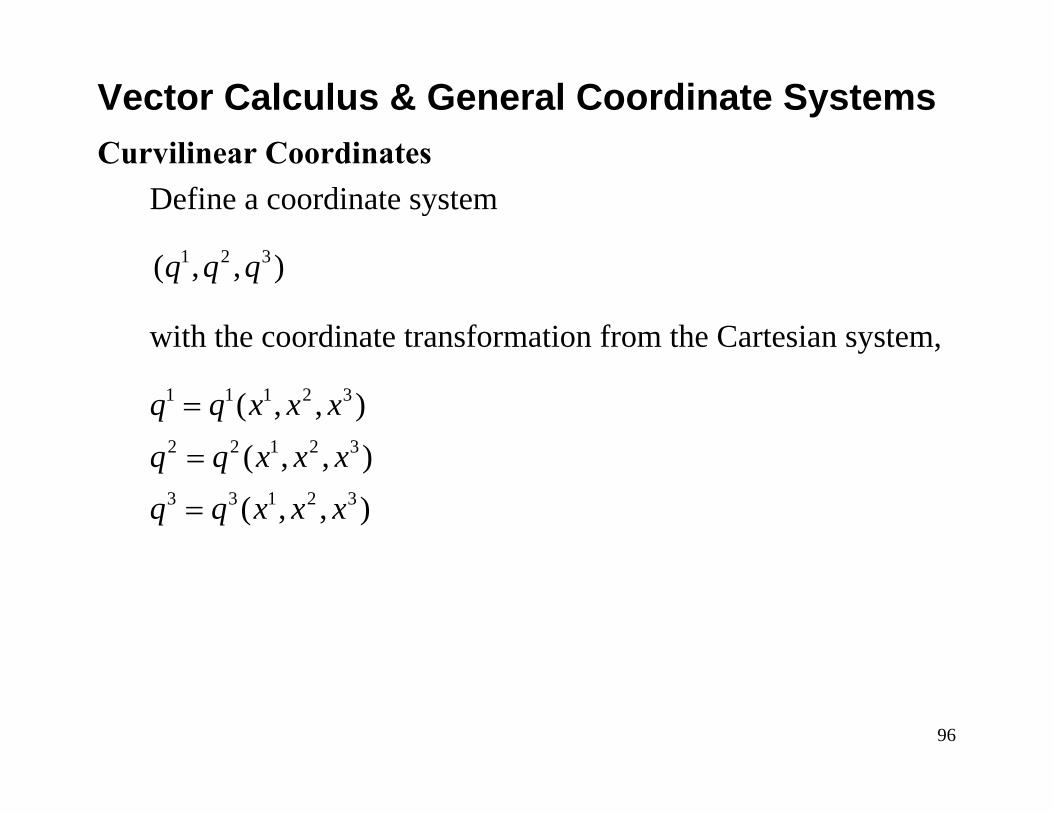
Curvilinear CoordinatesDefine a coordinate system

with the coordinate transformation from the Cartesian system,


1 2 3( , , )q q q

1 1 1 2 3

2 2 1 2 3

3 3 1 2 3

( , , )( , , )( , , )

q q x x xq q x x xq q x x x

=

=

=

97


2q

q1 = const

q3 = const

q2 = const

r

1q

3q

1x

2x

3x3q

∂∂

r

2q∂∂

r

1q∂∂

r

98

If the transformation is linear, it defines a Cartesian system. If the transformation is nonlinear, it defines a curvilinearsystem.The Jacobian of the transformation is defined by the following determinant,


1 1 1 1 2 3

1 2 3 1 1 1

2 2 2 1 2 3

1 2 3 2 2 2

3 3 3 1 2 3

1 2 3 3 3 3

j

i

x x x x x xq q q q q q

x x x x x x xJq q q q q q q

x x x x x xq q q q q q

∂ ∂ ∂ ∂ ∂ ∂∂ ∂ ∂ ∂ ∂ ∂

∂ ∂ ∂ ∂ ∂ ∂ ∂= = =

∂ ∂ ∂ ∂ ∂ ∂ ∂

∂ ∂ ∂ ∂ ∂ ∂∂ ∂ ∂ ∂ ∂ ∂

99

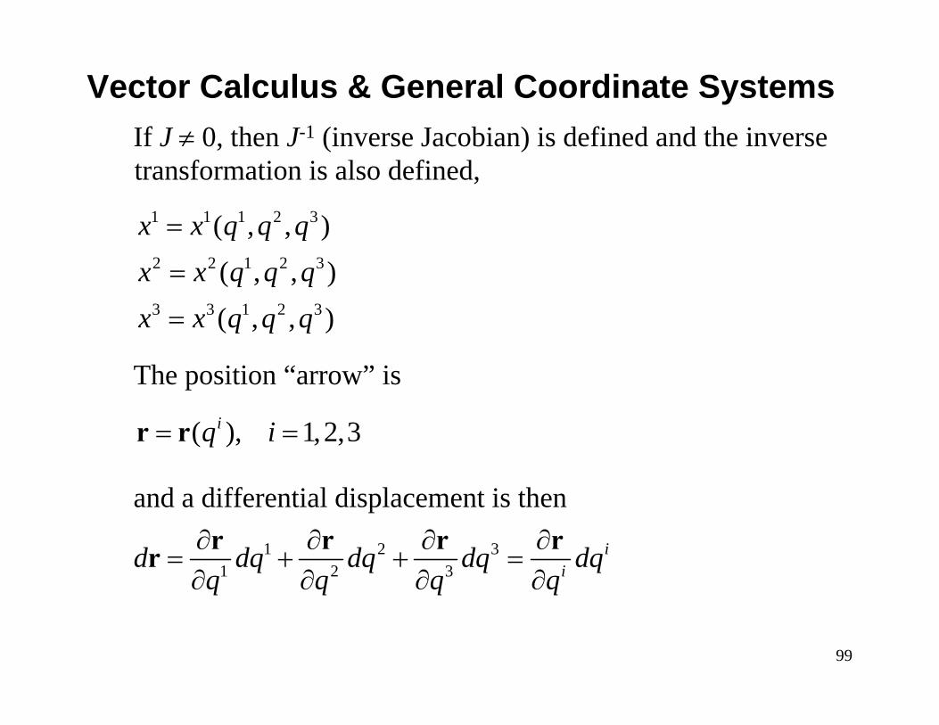
If J ≠ 0, then J-1 (inverse Jacobian) is defined and the inverse transformation is also defined,

The position “arrow” is

and a differential displacement is then


1 1 1 2 3

2 2 1 2 3

3 3 1 2 3

( , , )( , , )( , , )

x x q q qx x q q qx x q q q

=

=

=

( ), 1,2,3iq i= =r r

1 2 31 2 3

iid dq dq dq dq

q q q q∂ ∂ ∂ ∂

= + + =∂ ∂ ∂ ∂

r r r rr

100

The vectors are tangent to the coordinate curves defined by the intersection of the coordinate surfaces (qi = const). Using these vectors, we define a unitary basis,

Note, in general, the orientation and magnitude of the basis vectors are not constant, e.g.,


, 1,2,3i i iq

∂= =

∂re

/ iq∂ ∂r

101


Oblique-Cartesian system: Basis vectors have constant magnitude and orientation

Curvilinear system: Basis vectors generally have non-constant magnitude and orientation

102

The coordinate transformation was written for a general system in terms of the original Cartesian system. We almost always write the transformations in this manner. In terms of the original Cartesian system, the unitary basis is given by,

This is a linear system that is easily written in matrix format.The coefficient matrix is the Jacobian matrix,


ˆ , 1,2,3j

i ji i

x iq q

∂ ∂= = =

∂ ∂re i

1 1 2 1 3 111

1 2 2 2 3 22 2

1 3 2 3 3 33 3

ˆ/ / /ˆ/ / /ˆ/ / /

x q x q x qx q x q x qx q x q x q

⎡ ⎤⎡ ⎤∂ ∂ ∂ ∂ ∂ ∂⎡ ⎤ ⎢ ⎥⎢ ⎥⎢ ⎥ = ∂ ∂ ∂ ∂ ∂ ∂ ⎢ ⎥⎢ ⎥⎢ ⎥ ⎢ ⎥⎢ ⎥∂ ∂ ∂ ∂ ∂ ∂⎢ ⎥⎣ ⎦ ⎣ ⎦ ⎢ ⎥⎣ ⎦

iee ie i

103

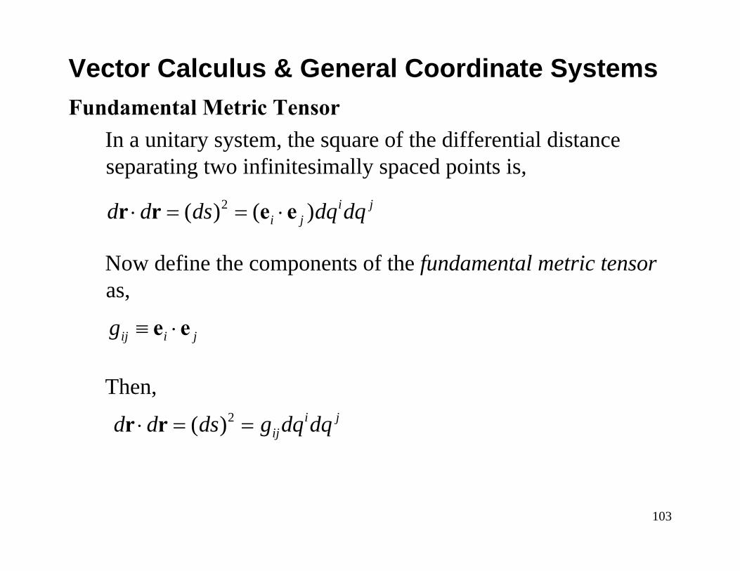
Fundamental Metric TensorIn a unitary system, the square of the differential distance separating two infinitesimally spaced points is,

Now define the components of the fundamental metric tensoras,

Then,


2( ) ( ) i ji jd d ds dq dq⋅ = = ⋅r r e e

ij i jg ≡ ⋅e e

2( ) i jijd d ds g dq dq⋅ = =r r

104

In matrix format, the fundamental metric tensor is,

Properties of the fundamental metric tensor:1. Symmetric, i.e.,

2. The norm (magnitude) of the unitary base vectors is,


i j j i ij jig g⋅ = ⋅ ↔ =e e e e

11 12 13

21 22 23

31 32 33

g g gG g g g

g g g

⎡ ⎤⎢ ⎥= ⎢ ⎥⎢ ⎥⎣ ⎦

1/ 2 1/ 2| | ( ) ( ) (no summation)i i i iig= ⋅ =e e e

105

3. Describes the curvature of the space, a) A flat space has no curvature and is called Euclidean.

In this case, all the gij components are constant.b) A curved space is called Riemannian In this case,

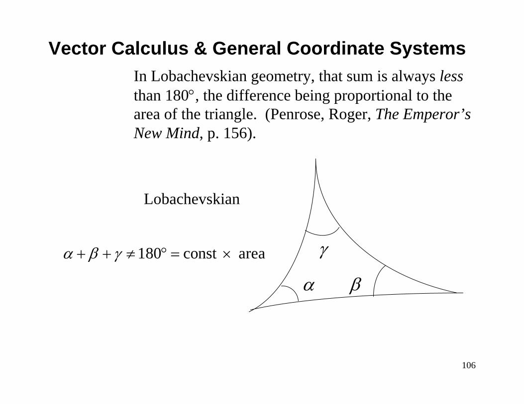
the gij components are not constant. An example is Lobachevskian space. This space has hyperbolic curvature.

We can compare these two spaces by looking at the geometry of a triangle in each. For Euclidean geometry, we know the sum of the interior angles of a triangle is always 180°.


α β

γ

Euclidean

180α β γ+ + = °

106

In Lobachevskian geometry, that sum is always lessthan 180°, the difference being proportional to the area of the triangle. (Penrose, Roger, The Emperor’s New Mind, p. 156).


βα

Lobachevskian

γ180 const areaα β γ+ + ≠ ° = ×

107

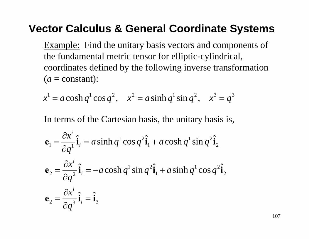
Example: Find the unitary basis vectors and components of the fundamental metric tensor for elliptic-cylindrical, coordinates defined by the following inverse transformation (a = constant):

In terms of the Cartesian basis, the unitary basis is,


1 1 2 2 1 2 3 3cosh cos , sinh sin ,x a q q x a q q x q= = =

1 2 1 21 1 21

1 2 1 22 1 22

2 33

ˆ ˆ ˆsinh cos cosh sin

ˆ ˆ ˆcosh sin sinh cos

ˆ ˆ

i

i

i

i

i

i

x a q q a q qqx a q q a q qqxq

∂= = +

∂

∂= = − +

∂

∂= =

∂

e i i i

e i i i

e i i

108

Components of the fundamental metric tensor are:

Components and BasesRecall,

Now set ,

With the definition for the components of G, we have,


2 2 1 2 2 2 1 2 211 1 1

22

33 12 21 13 31

[sinh ( )cos ( ) cosh ( )sin ( )

1, 0

g a q q q qg

g g g g g

= ⋅ = +== = = = =

e e

( ) ( )i ii i= ⋅ = ⋅a a e e a e e

j=a e( ) i

j j i= ⋅e e e e

109

Then according to the cogredient and contragredienttransformation laws raising and lowering of the indices is accomplished with the following,e j = gij ei and a j = gij ai

ej = gij ei and aj = gij ai .Note that when dealing with a unitary basis, cogredientcomponents and vectors are referred to as covariantcomponents and contragredient components and vectors are referred to as contravariant components.


ij i jg ≡ ⋅e e

ij i jg ≡ ⋅e e

contravariant component of the fundamental metric.covariant component of the fundamental metric.

110

Also, if we “dot” both sides of the ej transformation equation, (ej = gij ei) ⋅ ek, then we get the neat result

(4)For this relation, note the sum over i, e.g.,

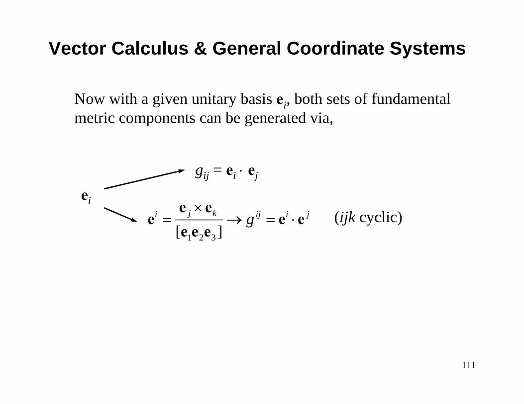
Now with a given unitary basis ei, both sets of fundamental metric components can be generated via,


k ikj ijg gδ =

1 11 21 311 11 21 31

2 12 22 321 11 21 31

1,

0.

g g g g g g

g g g g g g

δ

δ

= + + =

= + + =

111

Now with a given unitary basis ei, both sets of fundamental metric components can be generated via,


ei

gij = ei ⋅ ej

(ijk cyclic)1 2 3[ ]j ki ij i jg×

= → = ⋅e e

e e ee e e

112

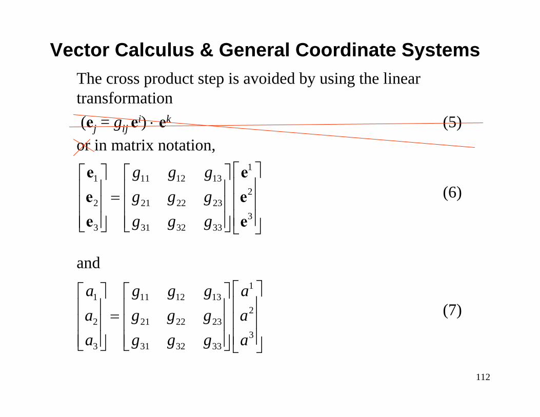
The cross product step is avoided by using the linear transformation (ej = gij ei) ⋅ ek (5)or in matrix notation,

(6)

and

(7)


11 11 12 13

22 21 22 23

33 31 32 33

g g gg g gg g g

⎡ ⎤⎡ ⎤ ⎡ ⎤⎢ ⎥⎢ ⎥ ⎢ ⎥= ⎢ ⎥⎢ ⎥ ⎢ ⎥⎢ ⎥⎢ ⎥ ⎢ ⎥⎣ ⎦ ⎣ ⎦ ⎣ ⎦

e ee ee e

11 11 12 13

22 21 22 23

33 31 32 33

a g g g aa g g g aa g g g a

⎡ ⎤⎡ ⎤ ⎡ ⎤⎢ ⎥⎢ ⎥ ⎢ ⎥= ⎢ ⎥⎢ ⎥ ⎢ ⎥⎢ ⎥⎢ ⎥ ⎢ ⎥⎣ ⎦ ⎣ ⎦ ⎣ ⎦

113

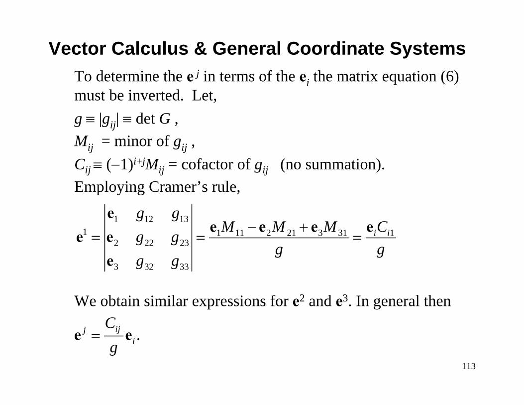
To determine the e j in terms of the ei the matrix equation (6) must be inverted. Let, g ≡ |gij| ≡ det G ,Mij = minor of gij , Cij ≡ (−1)i+jMij = cofactor of gij (no summation). Employing Cramer’s rule,

We obtain similar expressions for e2 and e3. In general then


1 12 131 1 11 2 21 3 31 1

2 22 23

3 32 33

i i

g gM M M Cg g

g gg g

− += = =

ee e e ee e

e

.ijji

Cg

=e e

114

Continuing in matrix format, you will probably recognize where this is leading, from the previous section on linear algebra. Since, gij = gji, the fundamental metric tensor is symmetric and Cij = Cji, then,

so

We designate the elements of G−1 with superscripts, i.e.,


[ ] [ ]11 Tj jij i iC G

g−⎡ ⎤ ⎡ ⎤⎡ ⎤= → =⎣ ⎦⎣ ⎦ ⎣ ⎦e e e e

11 .T

ijC Gg

−⎡ ⎤ =⎣ ⎦

1 .ijG g− ⎡ ⎤= ⎣ ⎦

115

So what have we accomplished with all this? If G = [gij] is known, we can use linear transformations and the rules of linear algebra to determine the dual basis and covariant components without formulae that involve cross products. In fact, knowing what we now know about systems of linear equations we could have anticipated this result from the matrix representation of Eq. (6), i.e.,

Another thing to note is the result in Eq. (4) is also anticipated since, in matrix notation, the Kronecker delta is the unit matrix,


[ ] [ ]1 .j ji iG G−⎡ ⎤ ⎡ ⎤= → =⎣ ⎦ ⎣ ⎦e e e e

116

Note that the product in Eq. (4) is just,


1.k ikj ijg g I GGδ −= ↔ =

1 0 00 1 0 .0 0 1

ijδ

⎡ ⎤⎢ ⎥⎡ ⎤ =⎣ ⎦ ⎢ ⎥⎢ ⎥⎣ ⎦

117

The General Permutation SymbolIn the Cartesian system, the cross product is well defined analytically and geometrically. What about general coordinates? We define the general permutation symbol by the operation

where

Using , we then write


(for a right-handed system)ki j ijk× =e e eE

1 2 3[ ].ijk i j k= × ⋅ ≡e e e e e eE

1 and .ijkijk ijk ijkg

gε ε= ≡E E

21 2 3det( ) [ ]ijg g= = e e e

118

Physical Components of a VectorRecall a physical component of a vector is defined by

Then,

Therefore, the physical component, in terms of the contravariant and covariant components is,


ˆˆ (no summation).i ii ia a=e e

ˆ ˆ ˆˆ

ˆ ˆ (no summation).| |

i ii i i i

i i i ii iii

i ii

a aga a a ag

⋅ = ⋅

= ⋅ → =

e e e eeee

ˆ ˆand similarily (no summation).i i iiii i ia a g a a g= =

119

Orthogonal Curvilinear Coordinate SystemsBecause of the many conveniences of orthogonal systems, most space-coordinate systems used in engineering analysis are orthogonal. Many of these systems are also curvilinear systems, in particular, the spherical and cylindrical systems with which you are familiar. In this section we will look at orthogonal curvilinear systems and how they relate to our original Cartesian system.

Scale FactorsDefine the scale factors


1 1 11 2 2 22 3 3 33| | , | | , | | .h g h g h g= = = = = =e e e

120

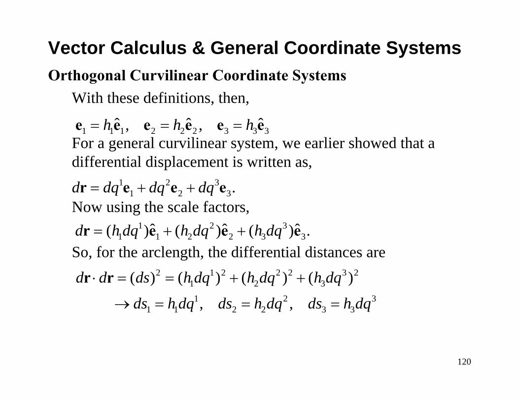
Orthogonal Curvilinear Coordinate SystemsWith these definitions, then,

For a general curvilinear system, we earlier showed that a differential displacement is written as,

Now using the scale factors,

So, for the arclength, the differential distances are


1 1 1 2 2 2 3 3 3ˆ ˆ ˆ, ,h h h= = =e e e e e e

1 2 31 2 3.d dq dq dq= + +r e e e

1 2 31 1 2 2 3 3ˆ ˆ ˆ( ) ( ) ( ) .d h dq h dq h dq= + +r e e e

2 1 2 2 2 3 21 2 31 2 3

1 1 2 2 3 3

( ) ( ) ( ) ( )

, ,

d d ds h dq h dq h dq

ds h dq ds h dq ds h dq

⋅ = = + +

→ = = =

r r

121


r dr

11 1( )h dq ds=

21 2( )h dq ds=

31 3( )h dq ds=

1q

3q

2q

r + dr

122

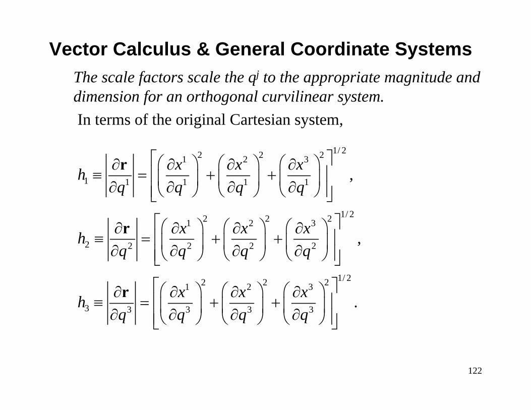
The scale factors scale the qj to the appropriate magnitude and dimension for an orthogonal curvilinear system.In terms of the original Cartesian system,


1/ 22 2 21 2 3

1 1 1 1 1

1/ 22 2 21 2 3

2 2 2 2 2

1/ 22 2 21 2 3

3 3 3 3 3

,

,

.

x x xhq q q q

x x xhq q q q

x x xhq q q q

⎡ ⎤⎛ ⎞ ⎛ ⎞ ⎛ ⎞∂ ∂ ∂ ∂≡ = + +⎢ ⎥⎜ ⎟ ⎜ ⎟ ⎜ ⎟∂ ∂ ∂ ∂⎢ ⎥⎝ ⎠ ⎝ ⎠ ⎝ ⎠⎣ ⎦

⎡ ⎤⎛ ⎞ ⎛ ⎞ ⎛ ⎞∂ ∂ ∂ ∂≡ = + +⎢ ⎥⎜ ⎟ ⎜ ⎟ ⎜ ⎟∂ ∂ ∂ ∂⎢ ⎥⎝ ⎠ ⎝ ⎠ ⎝ ⎠⎣ ⎦

⎡ ⎤⎛ ⎞ ⎛ ⎞ ⎛ ⎞∂ ∂ ∂ ∂≡ = + +⎢ ⎥⎜ ⎟ ⎜ ⎟ ⎜ ⎟∂ ∂ ∂ ∂⎢ ⎥⎝ ⎠ ⎝ ⎠ ⎝ ⎠⎣ ⎦

r

r

r

123

Differential Volume ElementIn many applications, especially finite-volume and finite-element methods, you often must determine the volume of a differential element. For instance, a finite-volume form of the mass conservation equation in fluid mechanics requires a computation of the flux of mass through the boundaries, which must balance the creation of mass inside the volume. In most applications, the differential cell (volume) is of some variableshape determined by a curvilinear coordinate system. Here we introduce a general expression for determining a differential volume.Recall how the scalar triple product is related to the volume ofa parallelepiped (with appropriate sign):


124

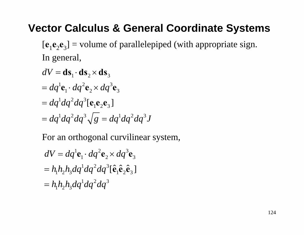
[e1e2e3] = volume of parallelepiped (with appropriate sign. In general,

For an orthogonal curvilinear system,


1 2 31 2 3

1 2 31 2 3

1 2 3

1 2 3 1 2 3

[ ]

dV

dq dq dq

dq dq dq

dq dq dq g dq dq dq J

= ⋅ ×

= ⋅ ×

=

= =

ds ds ds

e e e

e e e

1 2 31 2 31 2 3

1 2 3 1 2 31 2 3

1 2 3

ˆ ˆ ˆ[ ]

dV dq dq dq

h h h dq dq dq

h h h dq dq dq

= ⋅ ×

=

=

e e e

e e e

125

Finally, for the Cartesian system, the familiar result

Note we can gain a bit of insight into the physical meaning of the Jacobian J. Combining the general expression for the differential volume element with that for the Cartesian system, we find,

This shows that the Jacobian of the transformation is the ratio of a differential volume in the Cartesian system to that of the general system. You can also see (if you haven’t already discovered this) how the Jacobian is related to the fundamental metric, .i.e., .


1 2 3dV dx dx dx dx dy dz= =

1 2 3 1 2 3 .dV dx dy dzJdq dq dq dq dq dq

= =

J g=

Documents

Elements of Linear Algebra: Q&A - Home | University of ... · Elements of Linear Algebra: Q&A A matrix is a rectangular array of objects (elements that are numbers, functions,