Embed Size (px)
Citation preview
P. Wesseling
ELEMENTS OF
COMPUTATIONAL FLUID
DYNAMICS
Lecture notes WI 4011 Numerieke Stromingsleer
Copyright c©2001 by P. Wesseling
Faculty ITS
Applied Mathematics


Preface
The technological value of computational fluid dynamics has become undis-puted. A capability has been established to compute flows that can be inves-tigated experimentally only at reduced Reynolds numbers, or at greater cost,or not at all, such as the flow around a space vehicle at re-entry, or a loss-of-coolant accident in a nuclear reactor. Large commercial computational fluiddynamics computer codes have arisen, and found widespread use in industry.Users of these codes need to be familiar with the basic principles. It has beenobserved on numerous occasions, that even simple flows are not correctlypredicted by advanced computational fluid dynamics codes, if used withoutsufficient insight in both the numerics and the physics involved. This courseaims to elucidate some basic principles of computational fluid dynamics.
Because the subject is vast we have to confine ourselves here to just a few as-pects. A more complete introduction is given in Wesseling (2001), and othersources quoted there. Occasionally, we will refer to the literature for furtherinformation. But the student will be examined only about material presentedin these lecture notes.
Fluid dynamics is governed by partial differential equations. These may besolved numerically by finite difference, finite volume, finite element and spec-tral methods. In engineering applications, finite difference and finite volumemethods are predominant. We will confine ourselves here to finite differenceand finite volume methods.
Although most practical flows are turbulent, we restrict ourselves here tolaminar flow, because this book is on numerics only. The numerical principlesuncovered for the laminar case carry over to the turbulent case. Furthermore,we will discuss only incompressible flow. Considerable attention is given tothe convection-diffusion equation, because much can be learned from thissimple model about numerical aspects of the Navier-Stokes equations. Onechapter is devoted to direct and iterative solution methods.

II
Errata and MATLAB software related to a number of examples discussed inthese course notes may be obtained via the author’s website, to be found atta.twi.tudelft.nl/nw/users/wesseling
(see under “Information for students’ / “College WI4 011 Numerieke Stro-mingsleer”)
Delft, September 2001 P. Wesseling

Table of Contents
Preface . . . . . . . . . . . . . . . . . . . . . . . . . . . . . . . . . . . . . . . . . . . . . . . . . . . . . . . I
1. The basic equations of fluid dynamics . . . . . . . . . . . . . . . . . . . . . 11.1 Introduction . . . . . . . . . . . . . . . . . . . . . . . . . . . . . . . . . . . . . . . . . . . 11.2 Vector analysis . . . . . . . . . . . . . . . . . . . . . . . . . . . . . . . . . . . . . . . . . 21.3 The total derivative and the transport theorem . . . . . . . . . . . . . 41.4 Conservation of mass . . . . . . . . . . . . . . . . . . . . . . . . . . . . . . . . . . . 51.5 Conservation of momentum . . . . . . . . . . . . . . . . . . . . . . . . . . . . . . 71.6 The convection-diffusion equation . . . . . . . . . . . . . . . . . . . . . . . . 121.7 Summary of this chapter . . . . . . . . . . . . . . . . . . . . . . . . . . . . . . . . 14
2. The stationary convection-diffusion equation in one dimen-
sion . . . . . . . . . . . . . . . . . . . . . . . . . . . . . . . . . . . . . . . . . . . . . . . . . . . . . . . 152.1 Introduction . . . . . . . . . . . . . . . . . . . . . . . . . . . . . . . . . . . . . . . . . . . 152.2 Analytic aspects . . . . . . . . . . . . . . . . . . . . . . . . . . . . . . . . . . . . . . . . 162.3 Finite volume method . . . . . . . . . . . . . . . . . . . . . . . . . . . . . . . . . . . 20
3. The stationary convection-diffusion equation in two dimen-
sions . . . . . . . . . . . . . . . . . . . . . . . . . . . . . . . . . . . . . . . . . . . . . . . . . . . . . . 413.1 Introduction . . . . . . . . . . . . . . . . . . . . . . . . . . . . . . . . . . . . . . . . . . . 413.2 Singular perturbation theory . . . . . . . . . . . . . . . . . . . . . . . . . . . . . 423.3 Finite volume method . . . . . . . . . . . . . . . . . . . . . . . . . . . . . . . . . . . 51
4. The nonstationary convection-diffusion equation . . . . . . . . . . 614.1 Introduction . . . . . . . . . . . . . . . . . . . . . . . . . . . . . . . . . . . . . . . . . . . 614.2 A numerical example . . . . . . . . . . . . . . . . . . . . . . . . . . . . . . . . . . . 624.3 Convergence, consistency and stability . . . . . . . . . . . . . . . . . . . . 664.4 Fourier stability analysis . . . . . . . . . . . . . . . . . . . . . . . . . . . . . . . . 694.5 Numerical experiments . . . . . . . . . . . . . . . . . . . . . . . . . . . . . . . . . . 78
5. The incompressible Navier-Stokes equations . . . . . . . . . . . . . . 835.1 Introduction . . . . . . . . . . . . . . . . . . . . . . . . . . . . . . . . . . . . . . . . . . . 835.2 Equations of motion and boundary conditions . . . . . . . . . . . . . . 845.3 Spatial discretization on staggered grid . . . . . . . . . . . . . . . . . . . . 86

IV Table of Contents
5.4 Temporal discretization on staggered grid. . . . . . . . . . . . . . . . . . 925.5 Numerical experiments . . . . . . . . . . . . . . . . . . . . . . . . . . . . . . . . . . 97
6. Iterative solution methods . . . . . . . . . . . . . . . . . . . . . . . . . . . . . . . . 1056.1 Introduction . . . . . . . . . . . . . . . . . . . . . . . . . . . . . . . . . . . . . . . . . . . 1056.2 Direct methods for sparse systems . . . . . . . . . . . . . . . . . . . . . . . . 1086.3 Basic iterative methods . . . . . . . . . . . . . . . . . . . . . . . . . . . . . . . . . 1136.4 Krylov subspace methods . . . . . . . . . . . . . . . . . . . . . . . . . . . . . . . . 1226.5 Distributive iteration . . . . . . . . . . . . . . . . . . . . . . . . . . . . . . . . . . . 126
References . . . . . . . . . . . . . . . . . . . . . . . . . . . . . . . . . . . . . . . . . . . . . . . . . . . . 132
Index . . . . . . . . . . . . . . . . . . . . . . . . . . . . . . . . . . . . . . . . . . . . . . . . . . . . . . . . . 133

1. The basic equations of fluid dynamics
1.1 Introduction
Fluid dynamics is a classic discipline. The physical principles governing theflow of simple fluids and gases, such as water and air, have been understoodsince the times of Newton. Since about 1950 classic fluid dynamics finds itselfin the company of computational fluid dynamics. This newer discipline stilllacks the elegance and unification of its classic counterpart, and is in a stateof rapid development.
Good starting points for exploration of the Internet for material related tocomputational fluid dynamics are the following websites:
www.cfd-online.com/
www.princeton.edu/~gasdyn/fluids.html
and the ERCOFTAC (European Research Community on Flow, Turbulenceand Combustion) site:
imhefwww.epfl.ch/ERCOFTAC/
The author’s website ta.twi.tudelft.nl/users/wesseling also has somelinks to relevant websites.
Readers well-versed in theoretical fluid dynamics may skip the remainder ofthis chapter, perhaps after taking note of the notation introduced in the nextsection. But those less familiar with this discipline will find it useful to con-tinue with the present chapter.
The purpose of this chapter is:
• To introduce some notation that will be useful later;• To recall some basic facts of vector analysis;• To introduce the governing equations of laminar incompressible fluid dy-namics;• To explain that the Reynolds number is usually very large. In later chaptersthis will be seen to have a large impact on numerical methods.
2 1. The basic equations of fluid dynamics
1.2 Vector analysis
Cartesian tensor notation
We assume a right-handed Cartesian coordinate system (x1, x2, ..., xd) withd the number of space dimensions. Bold-faced lower case Latin letters de-note vectors, for example, x = (x1, x2, ..., xd). Greek letters denote scalars.In Cartesian tensor notation, which we shall often use, differentiation is de-noted as follows:
φ,α = ∂φ/∂xα .
Greek subscripts refer to coordinate directions, and the summation conven-tion is used: summation takes place over Greek indices that occur twice in aterm or product.
Examples
Inner product: u · v = uαvα =d∑
α=1uαvα
Laplace operator: ∇2φ = φ,αα =d∑
α=1∂2φ/∂x2
α
Note that uα + vα does not meand∑
α=1(uα + vα) (why?) 2
We will also use vector notation, instead of the subscript notation just ex-plained, and may write divu, if this is more elegant or convenient than thetensor equivalent uα,α; and sometimes we write gradφ or ∇φ for the vector(φ,1, φ,2, φ,3).
The Kronecker delta δαβ is defined by:
δ11 = δ22 = · · · = δdd = 1, δαβ = 0, α 6= β ,
where d is the number of space dimensions.
Divergence theorem
We will need the following fundamental theorem:
Theorem 1.2.1. For any volume V ⊂ Rd with piecewise smooth closed sur-
face S and any differentiable scalar field φ we have
1.2 Vector analysis 3
∫
V
φ,αdV =
∫
S
φnαdS ,
where n is the outward unit normal on S.
For a proof, see for example Aris (1962).
A direct consequence of this theorem is:
Theorem 1.2.2. (Divergence theorem).For any volume V ⊂ R
d with piecewise smooth closed surface S and anydifferentiable vector field u we have
∫
V
divudV =
∫
S
u · ndS ,
where n is the outward unit normal on S.
Proof. Apply Theorem 1.2.1 with φ,α = uα, α = 1, 2, ..., d successively andadd. 2
A vector field satisfying divu = 0 is called solenoidal.
The streamfunction
In two dimensions, if for a given velocity field u there exists a function ψsuch that
ψ,1 = −u2, ψ,2 = u1,
then such a function is called the streamfunction. For the streamfunctionto exist it is obviously necessary that ψ,12 = ψ,21; therefore we must haveu1,1 = −u2,2, or divu = 0. Hence, two-dimensional solenoidal vector fieldshave a streamfunction. The normal to an isoline ψ(x) = constant is parallelto ∇ψ = (ψ,1, ψ,2); therefore the vector u = (ψ,2,−ψ,1) is tangential tothis isoline. Streamlines are curves that are everywhere tangential to u. Wesee that in two dimensions the streamfunction is constant along streamlines.Later this fact will provide us with a convenient way to compute streamlinepatterns numerically.
Potential flow
The curl of a vector field is defined by
4 1. The basic equations of fluid dynamics
curlu =
u3,2 − u2,3
u1,3 − u3,1
u2,1 − u1,2
.
That is, the x1-component of the vector curlu is u3,2−u2,3, etc. Often, the curlis called rotation, and a vector field satisfying curlu = 0 is called irrotational.In two dimensions, the curl is obtained by putting the third component and∂/∂x3 equal to zero. This gives
curlu = u2,1 − u1,2 .
It can be shown (cf. Aris (1962)) that if a vector field u satisfies curlu = 0there exists a scalar field ϕ such that
u = gradϕ (1.1)
(or uα = ϕ,α). The scalar ϕ is called the potential, and flows with velocityfield u satisfying (1.1) are called potential flows or irrotational flows (sincecurl gradϕ = 0, cf. Exercise 1.2.3).
Exercise 1.2.1. Prove Theorem 1.2.1 for the special case that V is the unitcube.
Exercise 1.2.2. Show that curlu is solenoidal.
Exercise 1.2.3. Show that curl gradϕ = 0.
Exercise 1.2.4. Show that δαα = d.
1.3 The total derivative and the transport theorem
Streamlines
We repeat: a streamline is a curve that is everywhere tangent to the velocityvector u(t,x) at a given time t. Hence, a streamline may be parametrizedwith a parameter s such that a streamline is a curve x = x(s) defined by
dx/ds = u(t,x) .
1.4 Conservation of mass 5
The total derivative
Let x(t,y) be the position of a material particle at time t > 0, that at timet = 0 had initial position y. Obviously, the velocity field u(t,x) of the flowsatisfies
u(t,x) =∂x(t,y)
∂t. (1.2)
The time-derivative of a property φ of a material particle, called a mate-rial property (for example its temperature), is denoted by Dφ/Dt. This iscalled the total derivative. All material particles have some φ, so φ is definedeverywhere in the flow, and is a scalar field φ(t,x). We have
Dφ
Dt≡ ∂
∂tφ[t,x(t,y)] , (1.3)
where the partial derivative has to be taken with y constant, since the totalderivative tracks variation for a particular material particle. We obtain
Dφ
Dt=∂φ
∂t+∂xα(t,y)
∂t
∂φ
∂xα.
By using (1.2) we getDφ
Dt=∂φ
∂t+ uαφ,α .
The transport theorem
A material volume V (t) is a volume of fluid that moves with the flow andconsists permanently of the same material particles.
Theorem 1.3.1. (Reynolds’s transport theorem)For any material volume V (t) and differentiable scalar field φ we have
d
dt
∫
V (t)
φdV =
∫
V (t)
(∂φ
∂t+ div φu)dV . (1.4)
For a proof, see Sect. 1.3 of Wesseling (2001).
We are now ready to formulate the governing equations of fluid dynamics,which consist of the conservation laws for mass, momentum and energy.
1.4 Conservation of mass
Continuum hypothesis
The dynamics of fluids is governed by the conservation laws of classicalphysics, namely conservation of mass, momentum and energy. From these
6 1. The basic equations of fluid dynamics
laws partial differential equations are derived and, under appropriate cir-cumstances, simplified. It is customary to formulate the conservation lawsunder the assumption that the fluid is a continuous medium (continuum hy-pothesis). Physical properties of the flow, such as density and velocity canthen be described as time-dependent scalar or vector fields on R
2 or R3, for
example ρ(t,x) and u(t,x).
The mass conservation equation
The mass conservation law says that the rate of change of mass in an arbitrarymaterial volume V (t) equals the rate of mass production in V (t). This canbe expressed as
d
dt
∫
V (t)
ρdV =
∫
V (t)
σdV , (1.5)
where ρ(t,x) is the density of the material particle at time t and position x,and σ(t,x) is the rate of mass production per volume. In practice, σ 6= 0 onlyin multiphase flows, in which case (1.5) holds for each phase separately. Wetake σ = 0, and use the transport theorem to obtain
∫
V (t)
(∂ρ
∂t+ divρu)dV = 0 .
Since this holds for every V (t) the integrand must be zero:
∂ρ
∂t+ divρu = 0 . (1.6)
This is the mass conservation law, also called the continuity equation.
Incompressible flow
An incompressible flow is a flow in which the density of each material particleremains the same during the motion:
ρ[t,x(t,y)] = ρ(0,y) . (1.7)
HenceDρ
Dt= 0 .
Becausedivρu = ρdivu + uαρ,α ,
it follows from the mass conservation law (1.6) that

1.5 Conservation of momentum 7
divu = 0 . (1.8)
This is the form that the mass conservation law takes for incompressible flow.
Sometimes incompressibility is erroneously taken to be a property of the fluidrather than of the flow. But it may be shown that compressibility dependsonly on the speed of the flow, see Sect. 1.12 of Wesseling (2001). If the mag-nitude of the velocity of the flow is of the order of the speed of sound in thefluid (∼ 340 m/s in air at sea level at 15C, ∼ 1.4 km/s in water at 15C,depending on the amount of dissolved air) the flow is compressible; if thevelocity is much smaller than the speed of sound, incompressibility is a goodapproximation. In liquids, flow velocities anywhere near the speed of soundcannot normally be reached, due to the enormous pressures involved and thephenomenon of cavitation.
1.5 Conservation of momentum
Body forces and surface forces
Newton’s law of conservation of momentum implies that the rate of change ofmomentum of a material volume equals the total force on the volume. Thereare body forces and surface forces. A body force acts on a material particle,and is proportional to its mass. Let the volume of the material particle bedV (t) and let its density be ρ. Then we can write
body force = f bρdV (t) . (1.9)
A surface force works on the surface of V (t) and is proportional to area. Thesurface force working on a surface element dS(t) of V (t) can be written as
surface force = fsdS(t) . (1.10)
Conservation of momentum
The law of conservation of momentum applied to a material volume gives
d
dt
∫
V (t)
ρuαdV =
∫
V (t)
f bαdV +
∫
S(t)
fsαdS . (1.11)
By substituting φ = ρuα in the transport theorem (1.4), this can be writtenas
∫
V (t)
[∂ρuα
∂t+ (ρuαuβ),β
]
dV =
∫
V (t)
ρf bαdV +
∫
S(t)
fsαdS . (1.12)

8 1. The basic equations of fluid dynamics
It may be shown (see Aris (1962)) there exist nine quantities ταβ such that
fsα = ταβnβ , (1.13)
where ταβ is the stress tensor and n is the outward unit normal on dS. Byapplying Theorem 1.2.1 with φ replaced by ταβ and nα by nβ , equation (1.12)can be rewritten as
∫
V (t)
[∂ρuα
∂t+ (ρuαuβ),β
]
dV =
∫
V (t)
(ρf bα + ταβ,β)dV .
Since this holds for every V (t), we must have
∂ρuα
∂t+ (ρuαuβ),β = ταβ,β + ρf b
α , (1.14)
which is the momentum conservation law . The left-hand side is called theinertia term, because it comes from the inertia of the mass of fluid containedin V (t) in equation (1.11).
An example where f b 6= 0 is stratified flow under the influence of gravity.
Constitutive relation
In order to complete the system of equations it is necessary to relate therate of strain tensor to the motion of the fluid. Such a relation is called aconstitutive relation. A full discussion of constitutive relations would lead ustoo far. The simplest constitutive relation is (see Batchelor (1967))
ταβ = −pδαβ + 2µ(eαβ − 1
3∆δαβ) , (1.15)
where p is the pressure, δαβ is the Kronecker delta, µ is the dynamic viscosity,eαβ is the rate of strain tensor, defined by
eαβ =1
2(uα,β + uβ,α) ,
and∆ = eαα = divu .
The quantity ν = µ/ρ is called the kinematic viscosity. In many fluids andgases µ depends on temperature, but not on pressure. Fluids satisfying (1.15)are called Newtonian fluids. Examples are gases and liquids such as water andmercury. Examples of non-Newtonian fluids are polymers and blood.

1.5 Conservation of momentum 9
The Navier-Stokes equations
Substitution of (1.15) in (1.14) gives
∂ρuα
∂t+ (ρuαuβ),β = −p,α + 2[µ(eαβ − 1
3∆δαβ)],β + ρf b
α . (1.16)
These are the Navier-Stokes equations. The terms in the left-hand side aredue to the inertia of the fluid particles, and are called the inertia terms. Thefirst term on the right represents the pressure force that works on the fluidparticles, and is called the pressure term. The second term on the right rep-resents the friction force, and is called the viscous term. The third term onthe right is the body force.
Because of the continuity equation (1.6), one may also write
ρDuα
Dt= −p,α + 2[µ(eαβ − 1
3∆δαβ)],β + ρf b
α . (1.17)
In incompressible flows ∆ = 0, and we get
ρDuα
Dt= −p,α + 2(µeαβ),β + ρf b
α . (1.18)
These are the incompressible Navier-Stokes equations. If, furthermore, µ =constant then we can use uβ,αβ = uβ,βα = 0 to obtain
ρDuα
Dt= −p,α + µuα,ββ + ρf b
α . (1.19)
This equation was first derived by Navier (1823), Poisson (1831), de Saint-Venant (1843) and Stokes (1845). Its vector form is
ρDu
Dt= −∇p+ µ∇2u + ρf b ,
where ∇2 is the Laplace operator. The quantity
Du
Dt=∂u
∂t+ uαu,α
is sometimes written as
Du
Dt=∂u
∂t+ u · ∇u .
Making the equations dimensionless
In fluid dynamics there are exactly four independent physical units: thoseof length, velocity, mass and temperature, to be denoted by L,U,M and
10 1. The basic equations of fluid dynamics
Tr, respectively. From these all other units can be and should be derived inorder to avoid the introduction of superfluous coefficients in the equations.For instance, the appropriate unit of time is L/U ; the unit of force F followsfrom Newton’s law as MU2/L. Often it is useful not to choose these unitsarbitrarily, but to derive them from the problem at hand, and to make theequations dimensionless. This leads to the identification of the dimensionlessparameters that govern a flow problem. An example follows.
The Reynolds number
Let L and U be typical length and velocity scales for a given flow problem,and take these as units of length and velocity. The unit of mass is chosen asM = ρrL
3 with ρr a suitable value for the density, for example the density inthe flow at upstream infinity, or the density of the fluid at rest. Dimensionlessvariables are denoted by a prime:
x′
= x/L, u′
= u/U, ρ′
= ρ/ρr . (1.20)
In dimensionless variables, equation (1.16) takes the following form:
L
U
∂ρ′
u′
α
∂t+ (ρ
′
u′
αu′
β),β = − 1
ρrU2p,α +
2
ρrULµ(e
′
αβ − 1
3∆
′
δαβ),β +L
U2ρ
′
f bα ,
(1.21)where now the subscript , α stands for ∂/∂x
′
α, and e′
αβ = 12 (u
′
α,β + u′
β,α),
∆′
= e′
αα. We introduce further dimensionless quantities as follows:
t′
= Ut/L, p′
= p/ρrU2, (f b)
′
=L
U2f b. (1.22)
By substitution in (1.21) we obtain the following dimensionless form of theNavier-Stokes equations, deleting the primes:
∂ρuα
∂t+ (ρuαuβ),β = −p,α + 2Re−1(eαβ − 1
3∆δαβ),β + f b
α ,
where the Reynolds number Re is defined by
Re =ρrUL
µ.
The dimensionless form of (1.19) is, if ρ = constant = ρr,
Duα
Dt= −p,α + Re−1uα,ββ + f b
α . (1.23)
The transformation (1.20) shows that the inertia term is of order ρrU2/L
and the viscous term is of order µU/L2. Hence, Re is a measure of the ratio

1.5 Conservation of momentum 11
of inertial and viscous forces in the flow. This can also be seen immediatelyfrom equation (1.23). For Re ≫ 1 inertia dominates, for Re ≪ 1 friction (theviscous term) dominates. Both are balanced by the pressure gradient.
In the case of constant density, equations (1.23) and (1.8) form a com-plete system of four equations with four unknowns. The solution dependson the single dimensionless parameter Re only. What values does Re havein nature? At a temperature of 150C and atmospheric pressure, for air wehave for the kinematic viscosity µ/ρ = 1.5 ∗ 10−5 m2/s, whereas for wa-ter µ/ρ = 1.1 ∗ 10−6 m2/s. In the International Civil Aviation OrganizationStandard Atmosphere, µ/ρ = 4.9 ∗ 10−5 m2/s at an altitude of 12.5 km. Thisgives for the flow over an aircraft wing in cruise condition at 12.5 km al-titude with wing cord L = 3 m and U = 900 km/h: Re = 1.5 ∗ 107. In awindtunnel experiment at sea-level with L = 0.5 m and U = 25 m/s weobtain Re = 8.3 ∗ 105. For landing aircraft at sea-level with L = 3 m andU = 220 km/h we obtain Re = 1.2 ∗ 107. For a house in a light wind withL = 10 m and U = 0.5 m/s we have Re = 3.3 ∗ 105. Air circulation in aroom with L = 4 m and U = 0.1 m/s gives Re = 2.7 ∗ 104. A large shipwith L = 200 m and U = 7 m/s gives Re = 1.3 ∗ 108, whereas a yacht withL = 7 m and U = 3 m/s has Re = 1.9 ∗ 107. A small fish with L = 0.1 m andU = 0.2 m/s has Re = 1.8 ∗ 104.
All these very different examples have in common that Re ≫ 1, which isindeed almost the rule in flows of industrial and environmental interest. Onemight think that flows around a given shape will be quite similar for differentvalues of Re, as long as Re ≫ 1, but nothing is farther from the truth. AtRe = 107 a flow may be significantly different from the flow at Re = 105, inthe same geometry. This strong dependence on Re complicates predictionsbased on scaled down experiments. Therefore computational fluid dynamicsplays an important role in extrapolation to full scale. The rich variety of so-lutions of (1.23) that evolves as Re → ∞ is one of the most surprising andinteresting features of fluid dynamics, with important consequences for tech-nological applications. A ‘route to chaos’ develops as Re → ∞, resulting inturbulence. Intricate and intriguing flow patterns occur, accurately renderedin masterful drawings by Leonardo da Vinci, and photographically recordedin Hinze (1975), Nakayama and Woods (1988), Van Dyke (1982) and Hirsch(1988).
Turbulent flows are characterized by small rapid fluctuations of a seeminglyrandom nature. Smooth flows are called laminar. The transition form laminarto turbulent flow depends on the Reynolds number and the flow geometry.Very roughly speaking (!), for Re > 10000 flows may be assumed to be tur-bulent.
The complexity of flows used to be thought surprising, since the physics

12 1. The basic equations of fluid dynamics
underlying the governing equations is simply conservation of mass and mo-mentum. Since about 1960, however, it is known that the sweeping general-izations about determinism of Newtonian mechanics made by many scientists(notably Laplace) in the nineteenth century were wrong. Even simple classicnonlinear dynamical systems often exibit a complicated seemingly randombehavior, with such a sensitivity to initial conditions, that their long-termbehavior cannot be predicted in detail. For a discussion of the modern viewon (un-)predictability in Newtonian mechanics, see Lighthill (1986).
The Stokes equations
Very viscous flows are flows with Re ≪ 1. For Re ↓ 0 the system (1.23)simplifies to the Stokes equations. If we multiply (1.23) by Re and let Re ↓ 0,the pressure drops out, which cannot be correct, since we would have fourequations (Stokes and mass conservation) for three unknowns uα. It followsthat p = O(Re−1). We therefore substitute
p = Re−1p′
. (1.24)
From (1.24) and (1.22) it follows that the dimensional (physical) pressure isµUp
′
/L. Substitution of (1.24) in (1.23), multiplying by Re and letting Re ↓ 0gives the Stokes equations:
uα,ββ − p,α = 0 . (1.25)
These linear equations together with (1.8) were solved by Stokes (1851) forflow around a sphere. Surprisingly, the Stokes equations do not describe lowReynolds flow in two dimensions. This is called the Stokes paradox. See Sect.1.6 of Wesseling (2001) for the equations that govern low Reynolds flows intwo dimensions.
The governing equations of incompressible fluid dynamics are given by, if thedensity is constant, equations (1.23) and (1.8). This is the only situation tobe considerd in these lecture notes.
Exercise 1.5.1. Derive equation (1.17) from equation (1.16).
Exercise 1.5.2. What is the speed of sound and the kinematic viscosity inthe air around you? You ride your bike at 18 km/h. Compute your Reynoldsnumber based on a characteristic length (average of body length and width,say) of 1 m. Do you think the flow around you will be laminar or turbulent?
1.6 The convection-diffusion equation 13
1.6 The convection-diffusion equation
Conservation law for material properties
Let ϕ be a material property, i.e. a scalar that corresponds to a physical prop-erty of material particles, such as heat or concentration of a solute in a fluid,for example salt in water. Assume that ϕ is conserved and can change onlythrough exchange between material particles or through external sources. Letϕ be defined per unit of mass. Then the conservation law for ϕ is:
d
dt
∫
V (t)
ρϕdV =
∫
S(t)
f ·n dS +
∫
V (t)
qdV .
Here f is the flux vector, governing the rate of transfer through the surface,and q is the source term. For f we assume Fick’s law (called Fourier’s law ifϕ is temperature):
f = k grad ϕ ,
with k the diffusion coefficient. By arguments that are now familiar it followsthat
∂ρϕ
∂t+ div(ρϕu) = (kϕ,α),α + q . (1.26)
This is the convection-diffusion equation. The left-hand side represents trans-port of ϕ by convection with the flow, the first term at the right representstransport by diffusion.
By using the mass conservation law, equation (1.26) can be written as
ρDϕ
Dt= (kϕ,α),α + q . (1.27)
If we add a term rϕ to the left-hand side of (1.26) we obtain the convection-diffusion-reaction equation:
∂ρϕ
∂t+ div(ρϕu) + rϕ = (kϕ,α),α + q .
This equation occurs in flows in which chemical reactions take place. TheBlack-Scholes equation, famous for modeling option prices in mathematicalfinance, is also a convection-diffusion-reaction equation:
∂ϕ
∂t+ (1 − k)
∂ϕ
∂x+ kϕ =
∂2ϕ
∂x2.
We will not discuss the convection-diffusion-reaction equation, but only theconvection-diffusion equation.

14 1. The basic equations of fluid dynamics
Note that the momentum equation (1.19) comes close to being a convection-diffusion equation. Many aspects of numerical approximation in computa-tional fluid dynamics already show up in the numerical analysis of the rela-tively simple convection-diffusion equation, which is why we will devote twospecial chapters to this equation.
Dimensionless form
We can make the convection-diffusion equation dimensionless in the same wayas the Navier-Stokes equations. The unit for ϕ may be called ϕr. It is leftas an exercise to derive the following dimensionless form for the convection-diffusion equation (1.26):
∂ρϕ
∂t+ div(ρϕu) = (Pe−1ϕ,α),α + q , (1.28)
where the Peclet number Pe is defined as
Pe = ρ0UL/k0 .
We see that the Peclet number characterizes the balance between convectionand diffusion. For Pe ≫ 1 we have dominating convection, for Pe ≪ 1 diffu-sion dominates. If equation (1.28) stands for the heat transfer equation withϕ the temperature, then for air we have k ≈ µ/0.73. Therefore, for the samereasons as put forward in Sect. 1.5 for the Reynolds number, in computa-tional fluid dynamics Pe ≫ 1 is the rule rather than the exception.
Exercise 1.6.1. Derive equation (1.28).
1.7 Summary of this chapter
We have introduced Cartesian tensor notation, and have recalled some basicfacts from vector analysis. The transport theorem helps to express the con-servation laws for mass and momentum of a fluid particle in terms of partialdifferential equations. This leads to the incompressible Navier-Stokes equa-tions. Nondimensionalization leads to the identification of the dimensionlessparameter governing incompressible viscous flows, called the Reynolds num-ber. We have seen that the value of the Reynolds number is usually very highin flows of industrial and environmental interest. We have briefly touchedupon the phenomenon of turbulence, which occurs if the Reynolds numberis large enough. The convection-diffusion equation, which is the conservationlaw for material properties that are transported by convection and diffusion,

15
has been derived. Its dimensionless form gives rise to the dimensionless Pecletnumber.
Some self-test questions
Write down the divergence theorem.
What is the total derivative?
Write down the transport theorem.
Write down the governing equations of incompressible viscous flow.
Define the Reynolds number.
Write down the convection-diffusion-reaction equation.

2. The stationary convection-diffusion equation
in one dimension
2.1 Introduction
Although the one-dimensional case is of no practical use, we will devote aspecial chapter to it, because important general principles of CFD can beeasily analyzed and explained thoroughly in one dimension. We will pay spe-cial attention to difficulties caused by a large Peclet number Pe, which isgenerally the case in CFD, as noted in Sect. 1.6.
In this chapter we consider the one-dimensional stationary version of thedimensionless convection-diffusion equation (1.28) with ρ = 1:
duϕ
dx=
d
dx
(
εdϕ
dx
)
+ q(x) , x ∈ Ω ≡ (0, 1) , (2.1)
where the domain has been chosen to be the unit interval, and ε = 1/Pe. Forthe physical meaning of this equation, see Sect. 1.6
The purpose of this chapter is:
• To explain that a boundary value problem can be well-posed or ill-posed, andto identify boundary conditions that give a well-posed problem for Pe ≫ 1;
• To discuss the choice of outflow boundary conditions;
• To explain how the maximum principle can tell us whether the exact solu-tion is monotone;
• To explain the finite volume discretization method;
• To explain the discrete maximum principle that may be satisfied by thenumerical scheme;
• To study the local truncation error on nonuniform grids;

18 2. The stationary convection-diffusion equation in one dimension
• To show by means of the discrete maximum principle that although thelocal truncation error is relatively large at the boundaries and in the interiorof a nonuniform grid, nevertheless the global truncation error can be aboutas small as on a uniform grid;
• To show how by means of local grid refinement accuracy and computingwork can be made independent of the Peclet number;
• To illustrate the above points by numerical experiments;
• To give a few hints about programming in MATLAB.
2.2 Analytic aspects
Conservation form
The time-dependent version of (2.1) can be written as
∂ϕ
∂t= Lϕ+ q , Lϕ ≡ ∂uϕ
∂x− ∂
∂x
(
ε∂ϕ
∂x
)
.
Let us integrate over Ω:
d
dt
∫
Ω
ϕdΩ =
∫
Ω
LϕdΩ +
∫
Ω
qdΩ.
Since∫
Ω
LϕdΩ =
(
uϕ− ε∂ϕ
∂x
)∣
∣
∣
∣
1
0
, (2.2)
(where we define f(x)|ba ≡ f(b) − f(a)), we see that
d
dt
∫
Ω
ϕdΩ =
(
uϕ− ε∂ϕ
∂x
)∣
∣
∣
∣
1
0
+
∫
Ω
qdΩ.
Hence, if there is no transport through the boundaries x = 0, 1, and if thesource term q = 0, then
d
dt
∫
Ω
ϕdΩ = 0 .
Therefore∫
ΩϕdΩ is conserved. The total amount of ϕ, i.e.
∫
ΩϕdΩ, can
change only in time by transport through the boundaries x = 0, 1, and bythe action of a source term q. Therefore a differential operator such as L,whose integral over the domain Ω reduces to an integral over the boundary,is said to be in conservation form.
2.2 Analytic aspects 19
A famous example of a nonlinear convection equation (no diffusion) is theBurgers equation (named after the TUD professor J.M. Burgers, 1895–1981):
∂ϕ
∂t+
1
2
∂ϕ2
∂x= 0 . (2.3)
This equation is in conservation form. But the following version is not inconservation form:
∂ϕ
∂t+ ϕ
∂ϕ
∂x= 0 . (2.4)
An exact solution
Let u ≡ 1, ε = constant and q = 0. Then equation (2.1) becomes
dϕ
dx= ε
d2ϕ
dx2, x ∈ Ω ≡ (0, 1) , (2.5)
which can be solved analytically by postulating ϕ = eλx. Substitution in (2.5)shows this is a solution if
λ− ελ2 = 0 ,
hence λ = 0 or λ = 1/ε. Therefore the general solution is
ϕ(x) = A+Bex/ε , (2.6)
with A and B free constants, that must follow from the boundary conditions,in order to determine a unique solution. We see that precisely two boundaryconditions are needed.
Boundary conditions
For a second order differential equation, such as (2.1), two boundary con-ditions are required, to make the solution unique. A differential equationtogether with its boundary conditions is called a boundary value problem.We start with the following two boundary conditions, both at x = 0:
ϕ(0) = a,dϕ(0)
dx= b. (2.7)
The first condition, which prescribes a value for ϕ, is called a Dirichlet con-dition; the second, which prescribes a value for the derivative of ϕ, is calleda Neumann condition. The boundary conditions (2.7) are satisfied if the con-stants in (2.6) are given by A = a− εb, B = εb, so that the exact solutionis given by
ϕ(x) = a− εb+ εbex/ε . (2.8)

20 2. The stationary convection-diffusion equation in one dimension
Ill-posed and well-posed
We now show there is something wrong with boundary conditions (2.7) ifε ≪ 1. Suppose b is perturbed by an amount δb. The resulting perturbationin ϕ(1) is
δϕ(1) = εδbe1/ε .
We see that|δϕ(1)||δb| ≫ 1 if ε≪ 1 .
Hence, a small change in a boundary condition causes a large change in thesolution if ε ≪ 1. We assume indeed ε ≪ 1, for reasons set forth in Sect.1.6. Problems which have large sensitivity to perturbations of the boundarydata (or other input, such as coefficients and right-hand side) are called ill-posed. Usually, but not always, ill-posedness of a problem indicates a faultin the formulation of the mathematical model. The opposite of ill-posed iswell-posed. Since numerical approximations always involve perturbations, ill-posed problems can in general not be solved numerically with satisfactoryaccuracy, especially in more than one dimension (although there are specialnumerical methods for solving ill-posed problems with reasonable accuracy;this is a special field). In the present case ill-posedness is caused by wrongboundary conditions.
It is left to the reader to show in Exercise 2.2.2 that the following boundaryconditions:
ϕ(0) = a,dϕ(1)
dx= b. (2.9)
lead to a well-posed problem. The exact solution is now given by (verify this):
ϕ(x) = a+ εb(e(x−1)/ε − e−1/ε). (2.10)
Note that equation (2.5) corresponds to a velocity u = 1, so that x = 0 isan inflow boundary. Hence in (2.9) we have a Dirichlet boundary conditionat the inflow boundary and a Neumann boundary condition at the outflowboundary. If we assume u = −1, so that this is the other way around, thenthe problem is ill-posed as ε ≪ 1 with boundary conditions (2.9). This fol-lows from the result of Exercise 2.2.3. We conclude that it is wrong to give aNeumann condition at an inflow boundary.
Finally, let a Dirichlet condition is given at both boundaries:
ϕ(0) = a, ϕ(1) = b. (2.11)
The exact solution is
ϕ(x) = a+ (b − a)ex/ε − 1
e1/ε − 1(2.12)
2.2 Analytic aspects 21
The result of Exercise 2.2.4 shows that boundary conditions (2.11) give awell-posed problem.
To summarize: To obtain a well-posed problem, the boundary conditions mustbe correct.
Maximum principle
We rewrite equation (2.1) as
duϕ
dx− d
dx
(
εdϕ
dx
)
= q(x) , x ∈ Ω . (2.13)
Let q(x) < 0, ∀x ∈ Ω. In an interior extremum of the solution in a point x0
we have dϕ(x0)/dx = 0, so that
ϕ(x0)du(x0)
dx− ε
d2ϕ(x0)
dx2< 0.
Now suppose that du/dx = 0 (in more dimensions it suffices that divu = 0,which is satisfied in incompressible flows). Then d2ϕ(x0)/dx
2 > 0, so thatthe extremum cannot be a maximum. This result is strengthened to the caseq(x) ≤ 0, ∀x ∈ Ω, i.e. including the equality sign, in Theorem 2.4.1 ofWesseling (2001). Hence, if
udϕ
dx− ε
d2ϕ
dx2< 0, ∀x ∈ Ω ,
local maxima can occur only at the boundaries. This is called the maximumprinciple. By reversing signs we see that if q(x) ≤ 0, ∀x ∈ Ω there cannot bean interior minimum. If q(x) ≡ 0 there cannot be an interior extremum, sothat the solution is monotone (in one dimension). The maximum principlegives us important information about the solution, without having to deter-mine the solution. Such information is called a priori information.
If the exact solution has no local maximum or minimum, then “wiggles” (os-cillations) in a numerical solution are nor physical, but must be a numericalartifact.
This concludes our discussion of analytic aspects (especially for ε≪ 1) of theconvection-diffusion equation. We now turn to numerical solution methods.
Exercise 2.2.1. Show that equation (2.3) is in conservation form, and that(2.4) is not.
22 2. The stationary convection-diffusion equation in one dimension
Exercise 2.2.2. Show that the solution (2.10) satisfies
|δϕ(x)||δa| = 1,
|δϕ(x)||δb| < ε(1 + e−1/ε).
Hence, the solution is relatively insensitive to the boundary data a and b forall ε > 0.
Exercise 2.2.3. Show that with u = −1, ε = constant and q = 0 thesolution of equation (2.1) is given by
ϕ(x) = a+ bεe1/ε(1 − e−x/ε) ,
so thatδϕ(1)
δb= ε(e1/ε − 1) .
Why does this mean that the problem is ill-posed for ε≪ 1?
Exercise 2.2.4. Show that it follows from the exact solution (2.12) that
|δϕ(x)||δa| < 2 ,
|δϕ(x)||δb| < 1 .
2
2.3 Finite volume method
We now describe how equation (2.1) is discretized with the finite volumemethod. We rewrite (2.1) as
Lϕ ≡ duϕ
dx− d
dx
(
εdϕ
dx
)
= q, x ∈ Ω ≡ (0, 1) . (2.14)
Let x = 0 be an inflow boundary, i.e. u(0) > 0. As seen before, it would bewrong to prescribe a Neumann condition (if ε≪ 1), so we assume a Dirichletcondition:
ϕ(0) = a . (2.15)
Let x = 1 be an outflow boundary, i.e. u(1) > 0. We prescribe either aNeumann condition:
dϕ(1)/dx = b , (2.16)
or a Dirichlet condition:ϕ(1) = b . (2.17)
The finite volume method works as follows. The domain Ω is subdivided insegments Ωj , j = 1, · · · , J, as shown in the upper part of Fig. 2.1. The seg-ments are called cells or finite volumes or control volumes , and the segment

2.3 Finite volume method 23
1 j J
1 j J
Fig. 2.1. Non-uniform cell-centered grid (above) and vertex-centered grid (below).
length, denoted by hj , is called the mesh size. The coordinates of the cen-ters of the cells are called xj , the size of Ωj is called hj and the coordinateof the interface between Ωj and Ωj+1 is called xj+1/2. The cell centers arefrequently called grid points or nodes. This is called a cell-centered grid; thenodes are in the centers of the cells and there are no nodes on the bound-aries. In a vertex-centered grid one first distributes the nodes over the domainand puts nodes on the boundary; the boundaries of the control volumes arecentered between the nodes; see the lower part of Fig. 2.1. We continue witha cell-centered grid. We integrate equation (2.14) over Ωj and obtain:
∫
Ωj
LϕdΩ = F |j+1/2j−1/2 =
∫
Ωj
qdΩ ∼= hjqj ,
with F |j+1/2j−1/2 ≡ Fj+1/2 − Fj−1/2, Fj+1/2 = F (xj+1/2), F (x) ≡ uϕ− εdϕ/dx.
Often, F (x) is called the flux. The following scheme is obtained:
Lhϕj ≡ Fj+1/2 − Fj−1/2 = hjqj , j = 1, · · · , J . (2.18)
We will call uϕ the convective flux and εdϕ/dx the diffusive flux.
Conservative scheme
Summation of equation (2.18) over all cells gives
J∑
j=1
Lhϕj = FJ+1/2 − F1/2 . (2.19)
We see that only boundary fluxes remain, to that equation (2.19) mimics theconservation property (2.2) of the differential equation. Therefore the scheme(2.18) is called conservative. This property is generally beneficial for accuracyand physical realism.
24 2. The stationary convection-diffusion equation in one dimension
Discretization of the flux
To complete the discretization, the flux Fj+1/2 has to be approximated interms of neighboring grid function values; the result is called the numericalflux. Central discretization of the convection term is done by approximatingthe convective flux as follows:
(uϕ)j+1/2∼= uj+1/2ϕj+1/2, ϕj+1/2 =
1
2(ϕj + ϕj+1) . (2.20)
Since u(x) is a known coefficient, uj+1/2 is known. One might think thatbetter accuracy on nonuniform grids is obtained by linear interpolation:
ϕj+1/2 =hjϕj+1 + hj+1ϕj
hj + hj+1. (2.21)
Surprisingly, the scheme (2.18) is less accurate with (2.21) than with (2.20),
as we will see. This is one of the important lessons that can be learned fromthe present simple one-dimensional example.
Upwind discretization is given by
(uϕ)j+1/2∼= 1
2(uj+1/2 + |uj+1/2|)ϕj +
1
2(uj+1/2 − |uj+1/2|)ϕj+1 . (2.22)
This means that uϕ is biased in upstream direction (to the left for u > 0, tothe right for u < 0), which is why this is called upwind discretization.
The diffusive part of the flux is approximated by
(εdϕ
dx)j+1/2
∼= εj+1/2(ϕj+1 − ϕj)/hj+1/2, hj+1/2 =1
2(hj + hj+1) . (2.23)
Boundary conditions
At x = 0 we cannot approximate the diffusive flux by (2.23), since the nodex0 is missing. We use the Dirichlet boundary condition, and write:
(εdϕ
dx)1/2
∼= 2ε1/2(ϕ1 − a)/h1 . (2.24)
This is a one-sided approximation of (εdϕdx )1/2, which might impair the accu-
racy of the scheme. We will investigate later whether this is the case or not.The convective flux becomes simply
(uϕ)1/2∼= u1/2a . (2.25)
2.3 Finite volume method 25
Next, consider the boundary x = 1 . Assume we have the Neumann condition(2.16). The diffusive flux is given directly by the Neumann condition:
(εdϕ
dx)J+1/2
∼= εJ+1/2b. (2.26)
Since x = 1 is assumed to be an outflow boundary, we have uJ+1/2 > 0, sothat for the upwind convective flux (2.22) an approximation for ϕJ+1/2 is notrequired. For the central convective fluxes (2.20) or (2.21) we approximateϕJ+1/2 with extrapolation, using the Neumann condition:
ϕJ+1/2∼= ϕJ + hJb/2 . (2.27)
The Dirichlet condition (2.17) is handled in the same way as at x = 0.
The numerical scheme
The numerical flux as specified above can be written as
Fj+1/2 = β0jϕj + β1
j+1ϕj+1, j = 1, · · · , J − 1 ,
F1/2 = β11ϕ1 + γ0 , FJ+1/2 = β0
JϕJ + γ1 ,(2.28)
where γ0,1 are known terms arising from the boundary conditions. For eam-ple, for the upwind scheme we obtain the results specified in Exercise 2.3.2.
For future reference, we also give the coefficients for the central schemes. Forthe central scheme (2.20) we find:
β0j =
1
2uj+1/2 + (ε/h)j+1/2, j = 1, · · · , J − 1 ,
β1j+1 =
1
2uj+1/2 − (ε/h)j+1/2, j = 1, · · · , J − 1 , β1
1 = −2ε1/2/h1 ,
γ0 = (u1/2 + 2ε1/2/h1)a ,
β0J = uJ+1/2 , γ1 = uJ+1/2hJb/2 − εJ+1/2b (Neumann),
β0J = 2εJ+1/2/hJ , γ1 = (uJ+1/2 − 2εJ+1/2/hJ)b (Dirichlet).
(2.29)
For the central scheme (2.21) we find:
β0j =
hj+1
2hj+1/2uj+1/2 + (ε/h)j+1/2, j = 1, · · · , J − 1 ,
β1j+1 =
hj
2hj+1/2uj+1/2 − (ε/h)j+1/2, j = 1, · · · , J − 1 .
(2.30)
The other coefficients (at the boundaries) are the same as in equation (2.29).On a uniform grid the central schemes (2.29) and (2.30) are identical.
26 2. The stationary convection-diffusion equation in one dimension
Substitution of equations (2.66)–(2.30) in equation (2.18) gives the followinglinear algebraic system:
Lhϕj = α−1j ϕj−1 + α0
jϕj + α1jϕj+1 = qj , j = 1, · · · , J , (2.31)
with α−11 = α1
J = 0. This is called the numerical scheme or the finite volumescheme. Its coefficients are related to those of the numerical flux (2.66) –(2.30)by
α−1j = −β0
j−1 , j = 2, · · · , J ,α0
j = β0j − β1
j , j = 1, · · · , J ,α1
j = β1j+1 , j = 1, · · · , J − 1 .
(2.32)
The right-hand side is found to be
qj = hjqj , j = 2, · · · , J − 1 ,
q1 = h1q1 + γ0 , qJ = hJqJ − γ1 .(2.33)
Stencil notation
The general form of a linear scheme is
Lhϕj =∑
k∈K
αkjϕj+k = qj , (2.34)
with K some index set. For example, in the case of (2.34), K = −1, 0, 1.The stencil [Lh] of the operator Lh is a tableau of the coefficients of thescheme of the following form:
[Lh]j = [ α−1j α0
j α1j ] . (2.35)
We will see later that this is often a convenient way to specify the coefficients.Equation (2.34) is the stencil notation of the scheme.
The matrix of the scheme
In matrix notation the scheme can be denoted as
Ay = b , y =
ϕ1
...ϕJ
, b =
q1...qJ
, (2.36)
where A is the following tridiagonal matrix:

2.3 Finite volume method 27
A =
α01 α1
1 0 · · · 0
α−12 α0
2 α12
...
0. . .
. . .. . . 0
... α−1J−1 α0
J−1 α1J−1
0 · · · 0 α−1J α0
J
. (2.37)
In MATLAB, A is simply constructed as a sparse matrix by (taking note ofequation (2.32)):
A = spdiags([-beta0 beta0-beta1 beta1], -1:1, n, n);
with suitable definition of the algebraic vectors beta0 and beta1. This is usedin the MATLAB code cd1 and several other of the MATLAB codes that gowith this course. These programs are available at the author’s website; seethe Preface to these lecture notes.
Vertex-centered grid
In the interior of a vertex-centered grid the finite volume method works justas in the cell-centered case, so that further explanation is not necessary. Butat the boundaries the procedure is a little different. If we have a Dirichletcondition, for example at x = 0, then an equation for ϕ1 is not needed,because ϕ1 is prescribed (x1 is at the boundary, see Fig. 2.1). Suppose wehave a Neumann condition at x = 1. Finite volume integration over the lastcontrol volume (which has xJ as the right end point, see Fig. 2.1) gives:
LhϕJ ≡ FJ − FJ−1/2 = hJqJ ,
where we approximate FJ as follows, in the case of the central scheme forconvection, for example:
FJ = uJϕJ − εJb ,
where b is given in (2.16).
Symmetry
When the velocity u ≡ 0, the convection-diffusion equation reduces to thediffusion equation, also called heat equation. According to equations (2.66)—(2.30) we have in this case β1
j = −β0j−1, so that (2.32) gives α1
j = α−1j+1,
which makes the matrix A symmetric. This holds also in the vertex-centeredcase. Symmetry can be exploited to save computer memory and to makesolution methods more efficient. Sometimes the equations are scaled to makethe coefficients of size O(1); but this destroys symmetry, unless the samescaling factor is used for every equation.

28 2. The stationary convection-diffusion equation in one dimension
Two important questions
The two big questions asked in the numerical analysis of differential equationsare:• How well does the numerical solution approximate the exact solution ofequation (2.14)?• How accurately and efficiently can we solve the linear algebraic system(2.36)?These questions will come up frequently in what follows. In the ideal caseone shows theoretically that the numerical solution converges to the exactsolution as the mesh size hj ↓ 0. In the present simple case, where we havethe exact solution (2.6), we can check convergence by numerical experiment.
Numerical experiments on uniform grid
We take u = 1, ε constant, q = 0 and the grid cell-centered and uniform,with hj = h = 1/12. We choose Dirichlet boundary conditions (2.11) witha = 0.2, b = 1. The exact solution is given by (2.12). The numerical results inthis section have been obtained with the MATLAB code cd1 . Fig. 2.2 givesresults for two values of the Peclet number (remember that ε = 1/Pe). We see
0 0.2 0.4 0.6 0.8 10.2
0.3
0.4
0.5
0.6
0.7
0.8
0.9
1Pe=10, 12 cells
0 0.2 0.4 0.6 0.8 1−0.4
−0.2
0
0.2
0.4
0.6
0.8
1Pe=40, 12 cells
Fig. 2.2. Exact solution (—) and numerical solution (*).
a marked difference between the cases Pe = 10 and Pe = 40. The numericalsolution for Pe = 40 is completely unacceptable. We will now analyze whythis is so and look for remedies.

2.3 Finite volume method 29
The maximum principle
In Sect. 2.2 we saw that according to the maximum principle, with q = 0the solution of equation (2.14) cannot have local extrema in the interior.This is confirmed of course in Fig. 2.2. However, the numerical solution forPe = 40 shows local extrema. These undesirable numerical artifacts are oftencalled “wiggles”. It is desirable that the numerical scheme satisfies a similarmaximum principle as the differential equation, so that artificial wiggles areexcluded. This is the case for positive schemes, defined below. Let the schemebe written in stencil notation:
Lhϕj =∑
k∈K
αkjϕj+k = qj , j = 1, · · · , J .
Definition 2.3.1. The operator Lh is of positive type if
∑
k∈K
αkj = 0, j = 2, · · · , J − 1 (2.38)
andαk
j < 0, k 6= 0, j = 2, · · · , J − 1 . (2.39)
Note that a condition is put on the coefficients only in the interior. The fol-lowing theorem says that schemes of positive type satisfy a similar maximumprinciple as the differential equation.
Theorem 2.3.1. Discrete maximum principle.If Lh is of positive type and
Lhϕj ≤ 0, j = 2, · · · , J − 2 ,
then ϕj ≤ maxϕ1, ϕJ.Corollary Let conditions (2.38) and (2.39) also hold for j = J . Thenϕj ≤ ϕ1.
A formal proof is given in Sect. 4.4 of Wesseling (2001), but it is easy to seethat the theorem is true. Let K = −1, 0, 1. We have for every interiorgrid point xj :
ϕj ≤ w−1ϕj−1 + w1ϕj+1 , w±1 ≡ −α±1j /α0
j .
Since w1 + w1 = 1 and w±1 > 0, ϕj is a weighted average of its neighborsϕj−1 and ϕj+1. Hence, either ϕj < maxϕj−1, ϕj+1 or ϕj = ϕj−1 = ϕj+1.
Let us now see whether the scheme used for Fig. 2.2 is of positive type. Itsstencil is given by equation (2.67):
30 2. The stationary convection-diffusion equation in one dimension
[Lh] =
[
−1
2u− ε
h2ε
h
1
2u− ε
h
]
. (2.40)
We see that this scheme is of positive type if and only if
p < 2 , p ≡ |u|hε
. (2.41)
The dimensionless number p is called the mesh Peclet number.
For the left half of Fig. 2.2 we have p = 10/12 < 2, whereas for the righthalf p = 40/12 > 2, which explains the wiggles. In general, Pe = UL/ε andp = Uh/ε, so that p = Peh/L, with L the length of the domain Ω and Urepresentative of the size of u, for example U = max[u(x) : x ∈ Ω]. and forp < 2 we must choose h small enough: h/L < 2/Pe. Since in practice Pe isusually very large, as shown in Sect. 1.6, this is not feasible (certainly not inmore than one dimension), due to computer time and memory limitations.Therefore a scheme is required that is of positive type for all values of Pe.Such a scheme is obtained if we approximate the convective flux uϕ such thata non-positive contribution is made to α±1
j . This is precisely what the upwindscheme (2.22) is about. For the problem computed in Fig. 2.2 its stencil is,since u > 0:
[Lh] =[
−u− ε
hu+ 2
ε
h− ε
h
]
. (2.42)
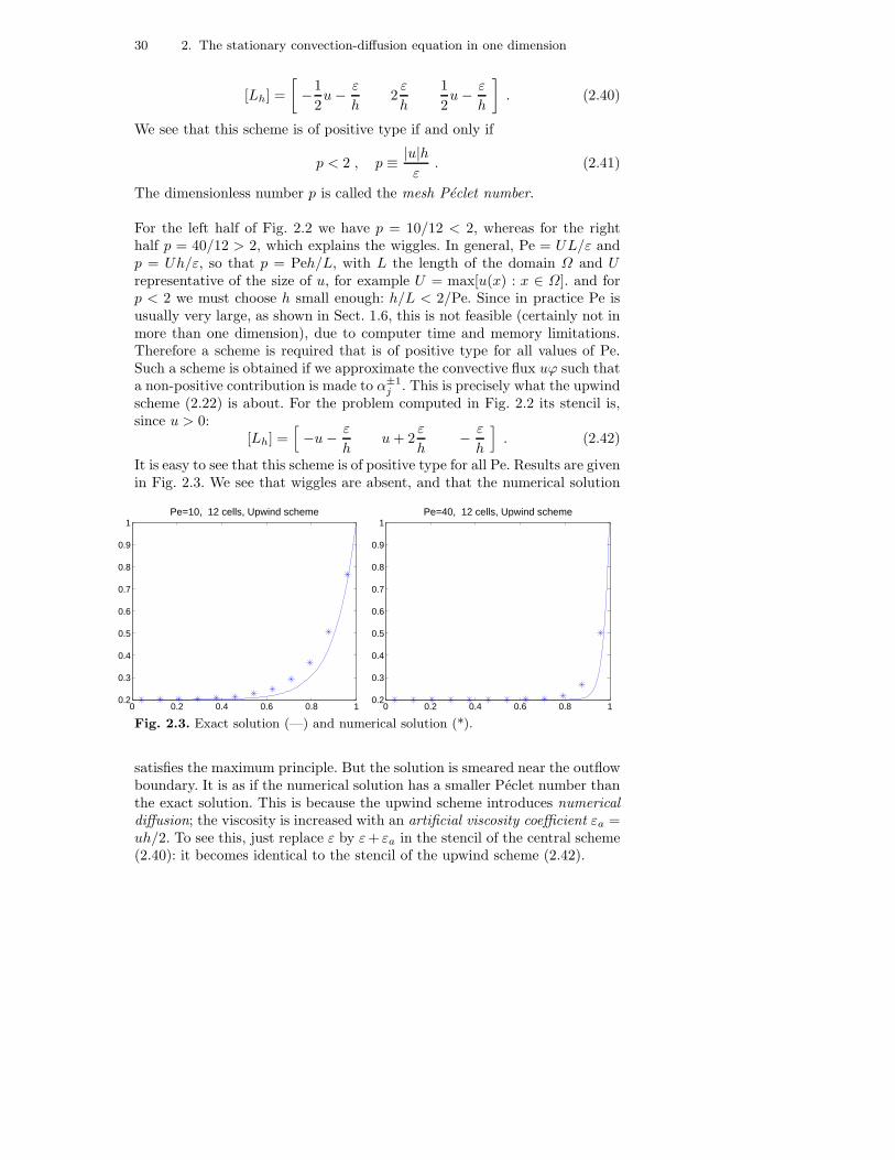
It is easy to see that this scheme is of positive type for all Pe. Results are givenin Fig. 2.3. We see that wiggles are absent, and that the numerical solution
0 0.2 0.4 0.6 0.8 10.2
0.3
0.4
0.5
0.6
0.7
0.8
0.9
1Pe=10, 12 cells, Upwind scheme
0 0.2 0.4 0.6 0.8 10.2
0.3
0.4
0.5
0.6
0.7
0.8
0.9
1Pe=40, 12 cells, Upwind scheme
Fig. 2.3. Exact solution (—) and numerical solution (*).
satisfies the maximum principle. But the solution is smeared near the outflowboundary. It is as if the numerical solution has a smaller Peclet number thanthe exact solution. This is because the upwind scheme introduces numericaldiffusion; the viscosity is increased with an artificial viscosity coefficient εa =uh/2. To see this, just replace ε by ε+ εa in the stencil of the central scheme(2.40): it becomes identical to the stencil of the upwind scheme (2.42).

2.3 Finite volume method 31
Local grid refinement
The preceding figures show for Pe = 40 a rapid variation of the exact solutionin a narrow zone near the outflow boundary x = 1. This zone is called aboundary layer. From the exact solution (2.13) it follows that the boundarylayer thickness δ satisfies
δ = O(ε) = O(Pe−1). (2.43)
(Landau’s order symbol O is defined later in this section). We will see laterhow to estimate the boundary layer thickness when an exact solution is notavailable. It is clear that to have reasonable accuracy in the boundary layer,the local mesh size must satisfy h < δ, in order to have sufficient resolution(i.e. enough grid points) in the boundary layer. This is not the case in theright parts of the preceding figures. To improve the accuracy we refine thegrid locally in the boundary layer. We define δ ≡ 6ε; the factor 6 is somewhatarbitrary and has been determined by trial and error. We put 6 equal cellsin (0, 1 − δ) and 6 equal cells in (1 − δ, 1). The result is shown in Fig. 2.4.Although the total number of cells remains the same, the accuracy of the
0 0.2 0.4 0.6 0.8 10.2
0.3
0.4
0.5
0.6
0.7
0.8
0.9
1Pe=40, 12 cells, Upwind scheme
0 0.2 0.4 0.6 0.8 10.2
0.3
0.4
0.5
0.6
0.7
0.8
0.9
1Pe=400, 12 cells, Upwind scheme
Fig. 2.4. Exact solution (—) and numerical solution (*) with local grid refinement;upwind scheme
upwind scheme has improved significantly. Even for Pe = 400, in which casethe boundary layer is very thin, the accuracy is good.
Fig. 2.5 gives results for the central scheme (2.20). Surprisingly, the wiggleswhich destroyed the accuracy in Fig. 2.2 have become invisible. In the refine-ment zone the local mesh Peclet number satisfies p = 1, which is less than 2,so that according to the maximum principle there can be no wiggles in therefinement zone (see equation (2.41) and the discussion preceding (2.41)).However, inspection of the numbers shows that small wiggles remain outsidethe refinement zone.
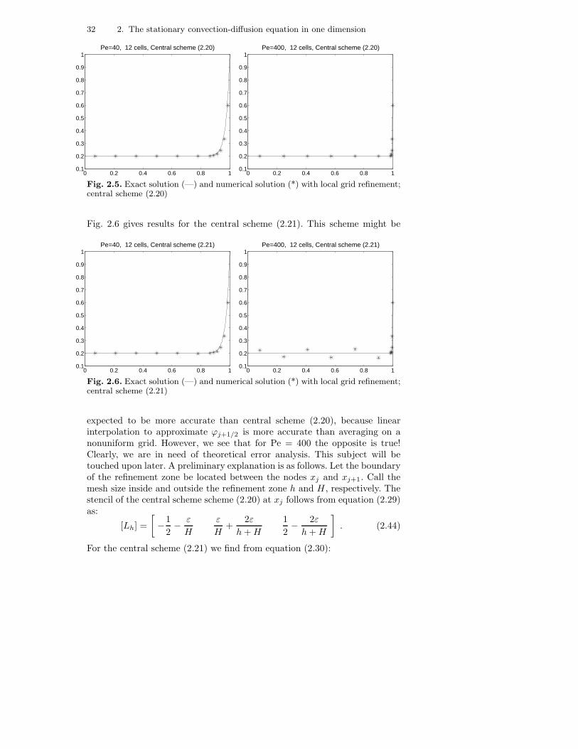
32 2. The stationary convection-diffusion equation in one dimension
0 0.2 0.4 0.6 0.8 10.1
0.2
0.3
0.4
0.5
0.6
0.7
0.8
0.9
1Pe=40, 12 cells, Central scheme (2.20)
0 0.2 0.4 0.6 0.8 10.1
0.2
0.3
0.4
0.5
0.6
0.7
0.8
0.9
1Pe=400, 12 cells, Central scheme (2.20)
Fig. 2.5. Exact solution (—) and numerical solution (*) with local grid refinement;central scheme (2.20)
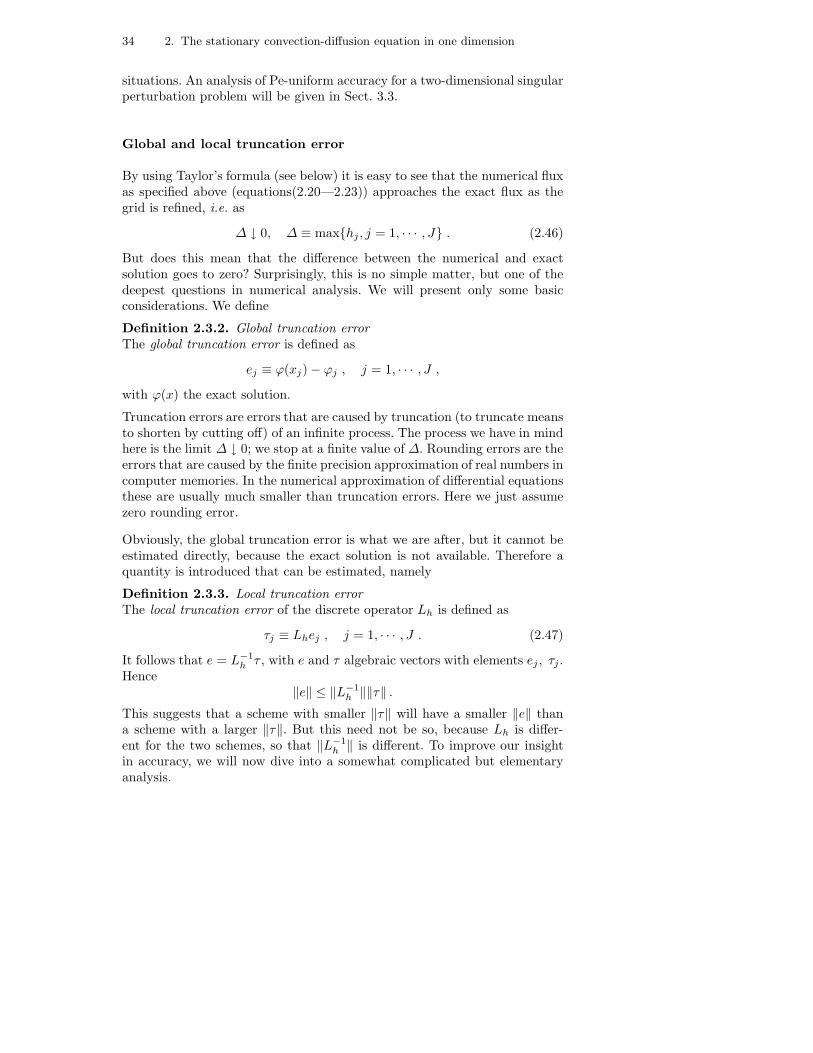
Fig. 2.6 gives results for the central scheme (2.21). This scheme might be
0 0.2 0.4 0.6 0.8 10.1
0.2
0.3
0.4
0.5
0.6
0.7
0.8
0.9
1Pe=40, 12 cells, Central scheme (2.21)
0 0.2 0.4 0.6 0.8 10.1
0.2
0.3
0.4
0.5
0.6
0.7
0.8
0.9
1Pe=400, 12 cells, Central scheme (2.21)
Fig. 2.6. Exact solution (—) and numerical solution (*) with local grid refinement;central scheme (2.21)
expected to be more accurate than central scheme (2.20), because linearinterpolation to approximate ϕj+1/2 is more accurate than averaging on anonuniform grid. However, we see that for Pe = 400 the opposite is true!Clearly, we are in need of theoretical error analysis. This subject will betouched upon later. A preliminary explanation is as follows. Let the boundaryof the refinement zone be located between the nodes xj and xj+1. Call themesh size inside and outside the refinement zone h and H , respectively. Thestencil of the central scheme scheme (2.20) at xj follows from equation (2.29)as:
[Lh] =
[
−1
2− ε
H
ε
H+
2ε
h+H
1
2− 2ε
h+H
]
. (2.44)
For the central scheme (2.21) we find from equation (2.30):

2.3 Finite volume method 33
[Lh] =
[
−1
2− ε
H− 1
2+
h
h+H+
ε
H+
2ε
h+H
H
h+H− 2ε
h+H
]
.
(2.45)According to definition 2.3.1, one of the necessary conditions for a positivescheme scheme is that the third element in the above stencils is non-positive.For ε ≪ 1 (and consequently h/H ≪ 1) this element is about 1/2 in (2.44)and 1 in (2.45), which is worse. Furthermore, in (2.45) the central element isnegative. We see that (2.45) deviates more from the conditions for a positivescheme than (2.44), so that it is more prone to wiggles.
Peclet-uniform accuracy and efficiency
The maximum norm of the error ej ≡ ϕ(xj) − ϕj is defined as
‖e‖∞ ≡ max|ej|, j = 1, · · · , J,
where ϕ(x) is the exact solution. Table 2.1 gives results. The number of cellsis the same as in the preceding figures. For Pe = 10 a uniform grid is used, forthe other cases the grid is locally refined, as before. We see that our doubts
Scheme Pe=10 Pe=40 Pe=400 Pe=4000Upwind .0785 .0882 .0882 .0882Central (2.20) .0607 .0852 .0852 .0852Central (2.21) .0607 .0852 .0856 .3657
Table 2.1. Maximum error norm; 12 cells.
about the central scheme (2.21) are confirmed. For the other schemes wesee that ‖e‖∞ is almost independent of Pe. This is due to the adaptive (i.e.Pe-dependent) local grid refinement in the boundary layer. Of course, sincethe number of cells J required for a given accuracy does not depend on Pe,computing work and storage are also independent of Pe. We may concludethat computing cost and accuracy are uniform in Pe.
This is an important observation. A not uncommon misunderstanding is thatnumerical predictions of high Reynolds (or Peclet in the present case) numberflows are inherently untrustworthy, because numerical discretization errors(‘numerical viscosity’) dominate the small viscous forces. This is not true,provided appropriate measures are taken, as was just shown. Local grid re-finement in boundary layers enables us to obtain accuracy independent ofthe Reynolds number. Because in practice Re (or its equivalent such as thePeclet number) is often very large (see Sect. 1.5) it is an important (but notimpossible) challenge to realize this also in more difficult multi-dimensional
34 2. The stationary convection-diffusion equation in one dimension
situations. An analysis of Pe-uniform accuracy for a two-dimensional singularperturbation problem will be given in Sect. 3.3.
Global and local truncation error
By using Taylor’s formula (see below) it is easy to see that the numerical fluxas specified above (equations(2.20—2.23)) approaches the exact flux as thegrid is refined, i.e. as
∆ ↓ 0, ∆ ≡ maxhj , j = 1, · · · , J . (2.46)
But does this mean that the difference between the numerical and exactsolution goes to zero? Surprisingly, this is no simple matter, but one of thedeepest questions in numerical analysis. We will present only some basicconsiderations. We define
Definition 2.3.2. Global truncation errorThe global truncation error is defined as
ej ≡ ϕ(xj) − ϕj , j = 1, · · · , J ,
with ϕ(x) the exact solution.
Truncation errors are errors that are caused by truncation (to truncate meansto shorten by cutting off) of an infinite process. The process we have in mindhere is the limit ∆ ↓ 0; we stop at a finite value of ∆. Rounding errors are theerrors that are caused by the finite precision approximation of real numbers incomputer memories. In the numerical approximation of differential equationsthese are usually much smaller than truncation errors. Here we just assumezero rounding error.
Obviously, the global truncation error is what we are after, but it cannot beestimated directly, because the exact solution is not available. Therefore aquantity is introduced that can be estimated, namely
Definition 2.3.3. Local truncation errorThe local truncation error of the discrete operator Lh is defined as
τj ≡ Lhej , j = 1, · · · , J . (2.47)
It follows that e = L−1h τ , with e and τ algebraic vectors with elements ej , τj .
Hence‖e‖ ≤ ‖L−1
h ‖‖τ‖ .This suggests that a scheme with smaller ‖τ‖ will have a smaller ‖e‖ thana scheme with a larger ‖τ‖. But this need not be so, because Lh is differ-ent for the two schemes, so that ‖L−1
h ‖ is different. To improve our insightin accuracy, we will now dive into a somewhat complicated but elementaryanalysis.

2.3 Finite volume method 35
Estimate of local truncation error in the interior
The purpose of the following elementary but laborious analysis is to eliminatetwo common misunderstandings. The first is that grids should be smooth foraccuracy; this is not true in general, at least not for positive schemes (Defi-nition 2.3.1). The second is that a large local truncation error at a boundarycauses a large global truncation error; this is also not true in general.
We begin with estimating the local truncation error. For simplicity u andε are assumed constant. We select the central scheme for convection. Thescheme (2.40) with a Dirichlet condition at x = 0 and a Neumann conditionat x = 1 (cf. equation (2.29)) can be written as
Lhϕ1 ≡(
u
2+
ε
h3/2+
2ε
h1
)
ϕ1 +
(
u
2− ε
h3/2
)
ϕ2 = h1q1 +
(
u+2ε
h1
)
a ,
Lhϕj ≡−(
u
2+
ε
hj−1/2
)
ϕj−1 + ε
(
1
hj−1/2+
1
hj+1/2
)
ϕj
+
(
u
2− ε
hj+1/2
)
ϕj+1 = hjqj , j = 2, · · · , J − 1 ,
LhϕJ ≡−(
u
2+
ε
hJ−1/2
)
ϕJ−1 +
(
u
2+
ε
hJ−1/2
)
ϕJ
=hJqJ −(u
2hJ − ε
)
b .
(2.48)
Taylor’s formula
To estimate the local truncation error we need Taylor’s formula:
f(x) = f(x0) +
n−1∑
k=1
1
k!
dkf(x0)
dxk(x− x0)
k +1
n!
dnf(ξ)
dxn(x− x0)
n (2.49)
for some ξ between x and x0. Of course, f must be sufficiently differentiable.This gives for the exact solution, writing ϕ(k) for dkϕ(x)/dxk,
ϕ(xj±1) = ϕ(xj) ± hj±1/2ϕ(1)(xj) +
1
2h2
j±1/2ϕ(2)(xj) ±
1
6h3
j±1/2ϕ(3)(xj)
+1
24h4
j±1/2ϕ(4)(xj) + O(h5
j±1/2) ,
(2.50)
where O is Landau’s order symbol, defined as follows:
36 2. The stationary convection-diffusion equation in one dimension
Definition 2.3.4. Landau’s order symbolA function f(h) = O(hp) if there exist a constant M independent of h and aconstant h0 > 0 such that
|f(h)|hp
< M, ∀h ∈ (0, h0) .
The relation f(h) = O(hp) is pronounced as “f is of order hp”.
Estimate of local truncation error, continued
We will now see that although we do not know the exact solution, we cannevertheless determine the dependence of τj on hj. We substitute (2.50) inLh(ϕ(xj), and obtain, after some tedious work that cannot be avoided, forj = 2, · · · , J − 1:
Lhϕ(xj) = Lhϕ(xj) + O(∆4) ,
Lhϕ(xj) ≡1
2qj(hj−1/2 + hj+1/2)
+
(
1
4uϕ(2) − 1
6εϕ(3)
)
(h2j+1/2 − h2
j−1/2)
+
(
1
12uϕ(3) − 1
24εϕ(4)
)
(h3j+1/2 + h3
j−1/2) ,
(2.51)
where ϕ(n) = dnϕ(xj)/dxn. We have
τj = Lhej = Lh[ϕ(xj) − ϕj ] = Lhϕ(xj) − hjqj + O(∆4) ,
so that we obtain:
τj =1
2qj(hj−1/2 − 2hj + hj+1/2)
+
(
1
4uϕ(2) − 1
6εϕ(3)
)
(h2j+1/2 − h2
j−1/2)
+
(
1
12uϕ(3) − 1
24εϕ(4)
)
(h3j+1/2 + h3
j−1/2) + O(∆4) .
(2.52)
The grid is called smooth if the mesh size hj varies slowly, or more precisely,if
|hj+1/2 − hj−1/2| = O(∆2) and |hj−1/2 − 2hj + hj+1/2| = O(∆3) .
Therefore on smooth grids τj = O(∆3), but on rough grids τj = O(∆).Therefore it is often thought that one should always work with smooth grids

2.3 Finite volume method 37
for better accuracy, but, surprisingly, this is not necessary in general. Wewill show why later. Note that the locally refined grid used in the precedingnumerical experiments is rough, but nevertheless the accuracy was found tobe satisfactory.
Estimate of local truncation error at the boundaries
For simplicity we now assume the grid uniform, with hj ≡ h. Let the schemebe cell-centered. We start with the Dirichlet boundary x = 0. Proceeding asbefore, we find using Taylor’s formula for ϕ(x2) in the first equation of (2.48),
Lhϕ(x1) = Lhϕ(x1) + O(h2) ,
Lhϕ(x1) ≡ (u + 2ε/h)ϕ(x1) − εϕ(1) +1
2q1h ,
where ϕ(1) = dϕ(x1)/dx, and ϕ(x) is the exact solution. We write
τ1 = Lh[ϕ(x1) − ϕ1] = Lhϕ(x1) − hq1 − (u+ 2ε/h)a+ O(h2)
= (u+ 2ε/h)[ϕ(x1) − a] − εϕ(1) − 1
2hq1 + O(h2) .
We use Taylor’s formula for a = ϕ(0):
a = ϕ(0) = ϕ(x1) −1
2hϕ(1) +
1
8h2ϕ(2) + O(h3)
and find
τ1 =h
4εϕ(2) + O(h2) . (2.53)
In the interior we have τj = O(h3) on a uniform grid, as seen from equation(2.52). However, it is not necessary to improve the local accuracy near aDirichlet boundary, which is one of the important messages of this section;we will show this below. But first we will estimate the local truncation errorat the Neumann boundary x = 1. By using Taylor’s formula for ϕ(xJ−1) inthe third equation of (2.48) we get
Lhϕ(xJ ) = Lhϕ(xJ ) + O(h3) ,
Lhϕ(xJ ) ≡ εϕ(1) +1
2qJh−
(u
4ϕ(2) − ε
6ϕ(3)
)
h2 + O(h3) ,
where ϕ(n) = dnϕ(xJ )/dxn. We write
τJ = Lh[ϕ(xJ ) − ϕJ ] = Lhϕ(xJ ) − hJqJ + (uhJ/2 − ε)b+ O(h3)
= εϕ(1) − qJh/2 − (uϕ(2)/4 − εϕ(3)/6)h2 + (uh/2 − ε)b + O(h3) .
We use Taylor’s formula for b = dϕ(1)/dx:

38 2. The stationary convection-diffusion equation in one dimension
b = ϕ(1) +1
2hϕ(2) +
1
8h2ϕ(3) + O(h3)
and find
τJ =1
24εϕ(3)h2 + O(h3) . (2.54)
Error estimation with the maximum principle
The student is not expected to be able to carry out the following error anal-ysis independently. This analysis is presented merely to make our assertionsabout accuracy on rough grids and at boundaries really convincing. We willuse the maximum principle to derive estimates of the global truncation errorfrom estimates of the local truncation error.
By e < E we mean ej < Ej , j = 1, · · · , J and by |e| we mean the gridfunction with values |ej |. We recall that the global and local truncation errorare related by
Lhe = τ . (2.55)
Suppose we have a grid function E, which will be called a barrier function,such that
LhE ≥ |τ | . (2.56)
We are going to show: |e| ≤ E. From (2.55) and (2.56) it follows that
Lh(±e− E) ≤ 0 .
Let the numerical scheme (2.48) satisfy the conditions of the corollary ofTheorem 2.3.1; this is the case if
|u|hj+1/2
ε< 2, j = 1, · · · , J − 1 . (2.57)
Then the corollary says
±ej − Ej ≤ ±e1 − E1, j = 2, · · · , J . (2.58)
Next we show that |e1| ≤ E1. From Lh(±e1 − E1) ≤ 0 it follows (with theuse of (2.58) for j = 2) that
a(±e1 − E1) ≤ b(±e2 − E2) ≤ b(±e1 − E1) ,
a = u/2 + 3ε/h1, b = ε/h1 − u/2 ,
where we assume h2 = h1. Note that 0 < b < a. Therefore ±e1 − E1 ≤ 0 ,hence |e1| ≤ E1. Substitution in (2.58) results in
|ej| ≤ Ej , j = 1, · · · , J . (2.59)
which we wanted to show. It remains to construct a suitable barrier functionE. Finding a suitable E is an art.

2.3 Finite volume method 39
Global error estimate on uniform grid
First, assume the grid is uniform: hj = h. We choose the barrier function asfollows:
Ej = Mψ(xj), ψ(x) ≡ 1 + 3x− x2 , (2.60)
with M a constant still to be chosen. We find (note that u > 0; otherwisethe boundary conditions would be ill-posed for ε≪ 1, as seen in Sect. 2.2):
Lhψ(x1) = u(1 + 3h− 5h2/4) +ε
h(2 + 3h2/2) > 2ε/h for h small enough ,
Lhψ(xj) = uh(3 − 2xj) + 2εh > 2εh, j = 2, · · · , J − 1 ,
Lhψ(xJ ) = ε(1 + 2h) + uh(1/2 + h) > ε .
According to equations (2.52)–(2.54) there exist constants M1 ,M2 ,M3 suchthat for h small enough
τ1 < M1h ,
τj < M2h3 , j = 2, · · · , J − 1 ,
τJ < M3h2 .
Hence, with
M =h2
εmaxM1/2, M2/2, M3
condition (2.56) is satisfied, so that
|e| < E = O(h2) .
This shows that the fact that the local truncation errors at the boundaries areof lower order than in the interior does not have a bad effect on the globaltruncation error.
Global error estimate on nonuniform grid
Next, we consider the effect of grid roughness. From equation (2.52) we seethat in the interior
τj = O(∆), ∆ = maxhj, j = 1, · · ·J .
We will show that nevertheless e = O(∆2), as for a uniform grid. The barrierfunction used before does not dominate τ sufficiently. Therefore we use thefollowing stratagem. Define the following grid functions:
µ1j ≡ h2
j , µ2j ≡
j∑
k=1
h3k−1/2 , µ3
j ≡j
∑
k=1
(h2k + h2
k−1)hk−1/2 ,
40 2. The stationary convection-diffusion equation in one dimension
where h0 ≡ 0. We find with Lh defined by (2.48) and ψk(x), k = 1, 2, 3smooth functions to be chosen later:
Lh(ψ1(xj)µ1j ) = εψ1(xj)(−2hj+1 + 4hj − 2hj−1) + (2.61)
+ εdψ1(xj)
dx− 1
2uψ1(xj)(h2
j−1 − h2j+1) + O(∆3) ,
Lh(ψ2(xj)µ2j ) = εψ2(xj)(h
2j−1/2 − h2
j+1/2) + O(∆3) , (2.62)
Lh(ψ3(xj)µ3j ) = εψ3(xj)(h
2j−1 − h2
j+1) + O(∆3) . (2.63)
We choose
ψ1 = −q(x)8ε
, ψ2 =1
6ϕ(3) − u
4εϕ(2) ,
ψ3 = −dψ1
dx+
u
2εψ1
and defineek
j ≡ ψk(xj)µkj , k = 1, 2, 3 .
Remembering (2.55), comparison of (2.61)–(2.63) with (2.52) shows that
Lh(ej − e1j − e2j − e3j) = O(∆3) . (2.64)
The right-hand side is of the same order as the local truncation error in theuniform grid case, and can be dominated by the barrier function (2.60) withM = C∆2, with C a constant that we will not bother to specify further. Forsimplicity we assume that h2 = h1 and hJ−1 = hJ , so that the situation atthe boundaries is the same as in the case of the uniform grid. Hence
|ej − e1j − e2j − e3j | < C∆2(1 + 3xj − x2j )
Since ekj = O(∆2) , k = 1, 2, 3 we find
ej = O(∆2) . (2.65)
which is what we wanted to show. Hence, the scheme defined by (2.48) hassecond order convergence on arbitrary grids, so that its widespread applica-tion is justified.
Vertex-centered grid
On a vertex-centered grid we have grid points on the boundary. Thereforethe Dirichlet boundary condition at x = 0 gives zero local truncation error,which is markedly better than (2.53). Furthermore, because the cell bound-aries are now midway between the nodes, the cell face approximation (2.20)is much more accurate. Indeed, the local truncation error is an order smaller
2.3 Finite volume method 41
on rough grids for vertex-centered schemes; we will not show this. Thereforeit is sometimes thought that vertex-centered schemes are more accurate thancell-centered schemes. But this is not so. In both cases, e = O(∆2). Becausethis is most surprising for cell-centered schemes, we have chosen to elaboratethis case. In practice, both types of grid are widely used.
Having come to the end of this chapter, looking again at the list of items thatwe wanted to cover given in Sect. 2.1 will help the reader to remind himselfof the main points that we wanted to emphasize.
Exercise 2.3.1. Derive equation (2.21). (Remember that linear interpola-tion is exact for functions of type f(x) = a+ bx).
Exercise 2.3.2. Assume u > 0. Show that for the upwind scheme the coef-ficients in the numerical flux are:
β0j = uj+1/2 + (ε/h)j+1/2, j = 1, · · · , J − 1 ,
β1j+1 = −(ε/h)j+1/2, j = 1, · · · , J − 1 , β1
1 = −2ε1/2/h1 ,
γ0 = (u1/2 + 2ε1/2/h1)a ,
β0J = uJ+1/2 , γ1 = −εJ+1/2b (Neumann),
β0J = uJ+1/2 + 2εJ+1/2/hJ , γ1 = −2εJ+1/2b/hJ (Dirichlet).
(2.66)
Exercise 2.3.3. Show that with ε and u constant on a uniform grid thestencil for the central scheme with Dirichlet boundary conditions is given by
[Lh]1 =
[
0 3ε
h+
1
2u
1
2u− ε
h
]
,
[Lh]j =
[
−1
2u− ε
h2ε
h
1
2u− ε
h
]
, j = 2, · · · , J − 1 ,
[Lh]J =
[
−1
2u− ε
h3ε
h− 1
2u 0
]
.
(2.67)
Exercise 2.3.4. Show that in the refinement zone the local mesh Pecletnumber satisfies p = 1.
Exercise 2.3.5. Derive equations (2.44) and (2.45).
Exercise 2.3.6. Implement a Neumann boundary condition at x = 1 in theMATLAB program cd1. Derive and implement the corresponding exact solu-tion. Study the error by numerical experiments. Implement wrong boundaryconditions: Neumann at inflow, Dirichlet at outflow. See what happens.

42
Exercise 2.3.7. In the program cd1 the size of the refinement zone isdel = 6/pe . Find out how sensitive the results are to changes in the factor6.
Exercise 2.3.8. Let xj = jh (uniform grid) and denote ϕ(xj) by ϕj . Show:
(ϕj − ϕj−1)/h =dϕ(xj)
dx− h
2
d2ϕ(ξ)
dx2, (2.68)
(ϕj+1 − ϕj−1)/(2h) =dϕ(xj)
dx+h2
6
d3ϕ(ξ)
dx3, (2.69)
(ϕj−1 − 2ϕj + ϕj+1)/h2 =
d2ϕ(xj)
dx2+h2
12
d4ϕ(ξ)
dx4, (2.70)
(2.71)
with ξ ∈ [xj−1 , xj+1].
Exercise 2.3.9. Show that
sinx√x
= O(√x).
Some self-test questions
When is the convection-diffusion equation in conservation form?
Write down the Burgers equation.
When do we call a problem ill-posed?
Formulate the maximum principle.
When is a finite volume scheme in conservation form?
What are cell-centered and vertex-centered grids?
What are the conditions for a scheme to be of positive type? Which desirable property do posi-tive schemes have?
Define the mesh-Peclet number.
Why is it important to have Peclet-uniform accuracy and efficiency?
Derive a finite volume scheme for the convection-diffusion equation.
Derive the condition to be satisfied by the step size h for the central scheme to be of positivetype on a uniform grid.
Define the global and local truncation error.
Derive the exact solution of the convection-diffusion equation.
Write down Taylor’s formula.

3. The stationary convection-diffusion equation
in two dimensions
3.1 Introduction
We will discuss only new aspects that did not come up in the one-dimensionalcase. The equation to be studied is the two-dimensional stationary convection-diffusion equation:
∂uϕ
∂x+∂vϕ
∂y− ∂
∂x
(
ε∂ϕ
∂x
)
− ∂
∂y
(
ε∂ϕ
∂y
)
= q(x, y) , (x, y) ∈ Ω ≡ (0, 1)×(0, 1) .
(3.1)Suitable boundary conditions are:
ϕ = f(x, y) on ∂Ωi (Dirichlet), (3.2)
ϕ = f(x, y) on ∂Ωo (Dirichlet) or (3.3)
∂ϕ
∂n= g(x, y) on ∂Ωo (Neumann), (3.4)
where n is the outward unit normal on the boundary ∂Ω, ∂Ωi is the inflowboundary (where u ·n < 0) and ∂Ωo is the remainder of ∂Ω, to be called theoutflow boundary.
We recall that ε = 1/Pe, with the Peclet number Pe ≫ 1. In the same wayas in Sect. 2.2 it can be shown that equation (3.1) is in conservation form.
As in one dimension, we have a maximum principle. We write (3.1) in thefollowing non-conservative form:
u∂ϕ
∂x+ v
∂ϕ
∂y− ∂
∂x
(
ε∂ϕ
∂x
)
− ∂
∂y
(
ε∂ϕ
∂y
)
= q ≡ q − ϕdivu . (3.5)
If q ≤ 0 then local maxima can only occur on the boundary ∂Ω. We willnot show this here; the interested reader may consult Sect. 2.4 of Wesseling(2001).

44 3. The stationary convection-diffusion equation in two dimensions
Purpose of this chapter
The purpose of this chapter is:
• To explain how singular perturbation theory can be used to predict wherefor Pe ≫ 1 thin layers (boundary layers) will occur without knowing the exactsolution;
• To show which boundary conditions are suitable for Pe ≫ 1;
• To introduce the finite volume method in two dimensions;
• To show how by means of local grid refinement accuracy and computingwork can be made independent of the Peclet number;
• To introduce the stencil of the scheme and to show how to generate itscoefficient matrix;
• To explain the discrete maximum principle in two dimensions;
• To illustrate the above points by numerical experiments.
Exercise 3.1.1. Show that equation (3.1) is in conservation form by usingTheorem 1.2.1.
3.2 Singular perturbation theory
Before discussing numerical schemes, we will consider singular perturbationtheory for the stationary convection-diffusion equation in two dimensions. Inview of our experience in the one-dimensional case, we expect when ε≪ 1 theoccurrence of thin layers in which the solution varies rapidly. Such layers arecalled boundary layers. As seen in Chapt. 2, local grid refinement is requiredin boundary layers for accuracy. Therefore it is necessary to know whereboundary layers occur and the dependence of their thickness on ε. In Chapt.2 this information was deduced from the exact solution; however, in generalthe exact solution is not available, of course. But the required information isprovided by singular perturbation theory, also called boundary layer theory.The boundary layer concept was first introduced by Ludwig Prandtl in 1904,but the mathematical foundation was developed in the middle of the lastcentury.
3.2 Singular perturbation theory 45
Subcharacteristics
When ε ≪ 1 it is natural to approximate (3.1) by putting ε = 0, so that weobtain, switching to nonconservative form:
u∂ϕ
∂x+ v
∂ϕ
∂y= q , q = q − ϕdivu . (3.6)
This is the convection equation. Let us define curves called characteristics inΩ space by relations x = x(s) y = y(s), satisfying
dx
ds= u ,
dy
ds= v . (3.7)
For the derivative along the curve we have
dϕ
ds=∂ϕ
∂x
dx
ds+∂ϕ
∂y
dy
ds= u
∂ϕ
∂x+ v
∂ϕ
∂y.
Therefore equation (3.6) reduces to
dϕ
ds= q . (3.8)
We see that in the homogeneous case q = 0 the solution ϕ is constant alongthe characteristics, which is why these curves are important. When ε > 0 wedo not have ϕ constant on the characteristics, but as we will see, these curvesstill play an important role when ε≪ 1. To avoid confusion, when ε > 0 thecharacteristics are called subcharacteristics.
A paradox
Let the pattern of streamlines (i.e. (sub)characteristics) be qualitatively as inFig. 3.1. The characteristic C1 intersects the boundary in points P1 and P2.Here a boundary condition is given, according to equations (3.2)—(3.4). OnC1 we have ϕ = constant = ϕ(C1). It is clear that in general ϕ(C1) cannot sat-isfy simultaneously the boundary conditions in P1 and in P2. For example, letϕ(P1) 6= ϕ(P2) be prescribed by a Dirichlet condition at y = 0 and at x = 1.Do we have ϕ(C1) = ϕ(P1) or ϕ(C1) = ϕ(P2) or ϕ(C1) = (ϕ(P1) + ϕ(P2))/2or something else? What value to take for ϕ(C1)? The difficulty has to dowith the change of type that the partial differential equation (3.1) undergoeswhen ε = 0: for ε > 0 it is elliptic, for ε = 0 it is hyperbolic. It is clearthat we cannot get a good approximation to equation (3.1) for ε ↓ 0 by sim-ply deleting the small diffusion term. This paradoxical situation has baffledmathematicians in the nineteenth century, who found the drag of a body inan ideal fluid (zero viscosity) to be zero, whereas in physical experimentsthe drag around bluff bodies was found to be appreciable, even at very high
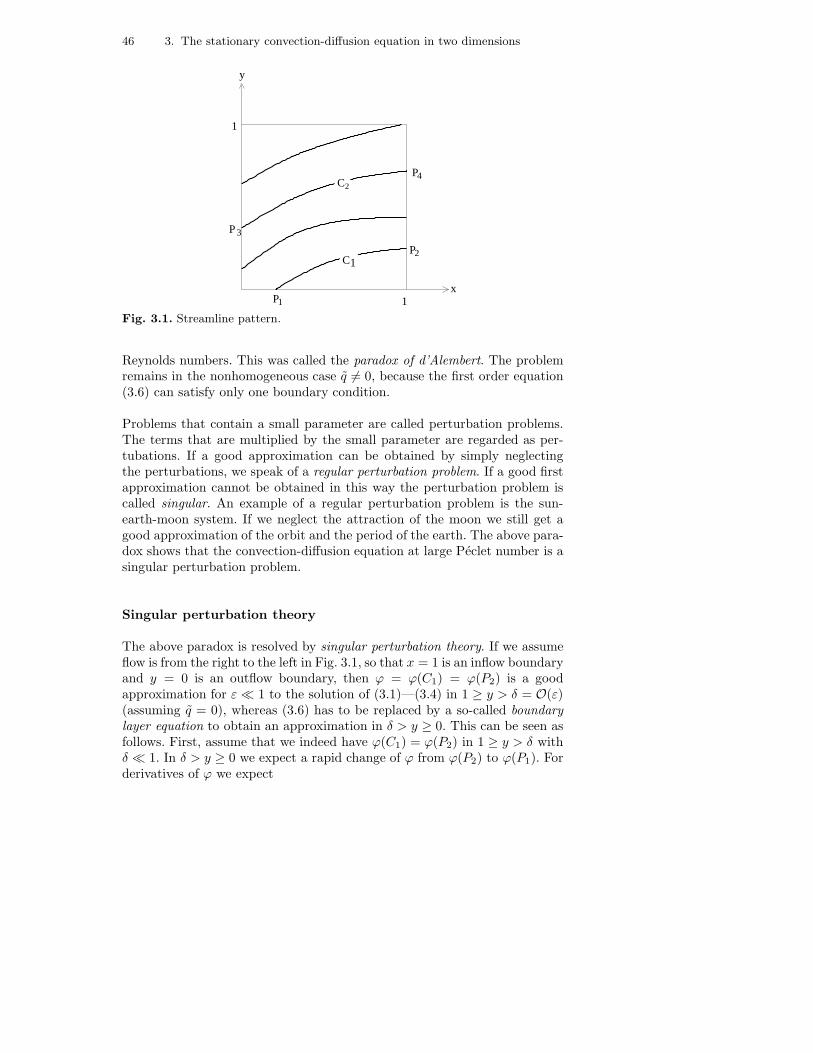
46 3. The stationary convection-diffusion equation in two dimensions
x
y
1
1
C
C1
2
P
P
P
P
3
1
2
4
Fig. 3.1. Streamline pattern.
Reynolds numbers. This was called the paradox of d’Alembert. The problemremains in the nonhomogeneous case q 6= 0, because the first order equation(3.6) can satisfy only one boundary condition.
Problems that contain a small parameter are called perturbation problems.The terms that are multiplied by the small parameter are regarded as per-tubations. If a good approximation can be obtained by simply neglectingthe perturbations, we speak of a regular perturbation problem. If a good firstapproximation cannot be obtained in this way the perturbation problem iscalled singular. An example of a regular perturbation problem is the sun-earth-moon system. If we neglect the attraction of the moon we still get agood approximation of the orbit and the period of the earth. The above para-dox shows that the convection-diffusion equation at large Peclet number is asingular perturbation problem.
Singular perturbation theory
The above paradox is resolved by singular perturbation theory. If we assumeflow is from the right to the left in Fig. 3.1, so that x = 1 is an inflow boundaryand y = 0 is an outflow boundary, then ϕ = ϕ(C1) = ϕ(P2) is a goodapproximation for ε ≪ 1 to the solution of (3.1)—(3.4) in 1 ≥ y > δ = O(ε)(assuming q = 0), whereas (3.6) has to be replaced by a so-called boundarylayer equation to obtain an approximation in δ > y ≥ 0. This can be seen asfollows. First, assume that we indeed have ϕ(C1) = ϕ(P2) in 1 ≥ y > δ withδ ≪ 1. In δ > y ≥ 0 we expect a rapid change of ϕ from ϕ(P2) to ϕ(P1). Forderivatives of ϕ we expect
3.2 Singular perturbation theory 47
∂mϕ
∂ym= O(δ−m) , (3.9)
so that perhaps the diffusion term in (3.1) cannot be neglected in the bound-ary layer; this will depend on the size of δ. Assume
δ = O(εα) , (3.10)
with α to be determined. In order to exhibit the dependence of the magnitudeof derivatives on ε we introduce a stretched coordinate y:
y = yε−α , (3.11)
which is chosen such that y = O(1) in the boundary layer. We take ε constantfor simplicity. It follows from (3.9)—(3.11) that
∂mϕ
∂ym= O(1) (3.12)
in the boundary layer. In the stretched coordinate, equation (3.1) becomes
∂uϕ
∂x+ ε−α ∂vϕ
∂y− ε
∂2ϕ
∂x2− ε1−2α ∂
2ϕ
∂y2= 0 . (3.13)
Letting ε ↓ 0 and using (3.12), equation (3.13) takes various forms, dependingon α. The correct value of α follows from the requirement, that the solutionof the ε ↓ 0 limit of equation (3.13) satisfies the boundary condition at y = 0,and the so-called matching principle.
Matching principle
As y increases, the solution of (the ε ↓ 0 limit of) equation (3.13) has tosomehow join up with the solution of (3.6), i.e. approach the value ϕ(C1).In singular perturbation theory this condition is formulated precisely, and isknown as the matching principle:
limy→∞
ϕinner(x, y) = limy↓0
ϕouter(x, y) .
Here ϕinner, also called the inner solution, is the solution of the inner equationor boundary layer equation, which is the limit as ε ↓ 0 of equation (3.13) forthe correct value of α, which we are trying to determine. Furthermore, ϕouter,also called the outer solution, is the solution of the outer equation, which isthe limit as ε ↓ 0 of the original equation, i.e. equation (3.6). The matchingprinciple becomes
ϕinner(x,∞) = g(x) ≡ limy↓0
ϕouter(x, y) . (3.14)
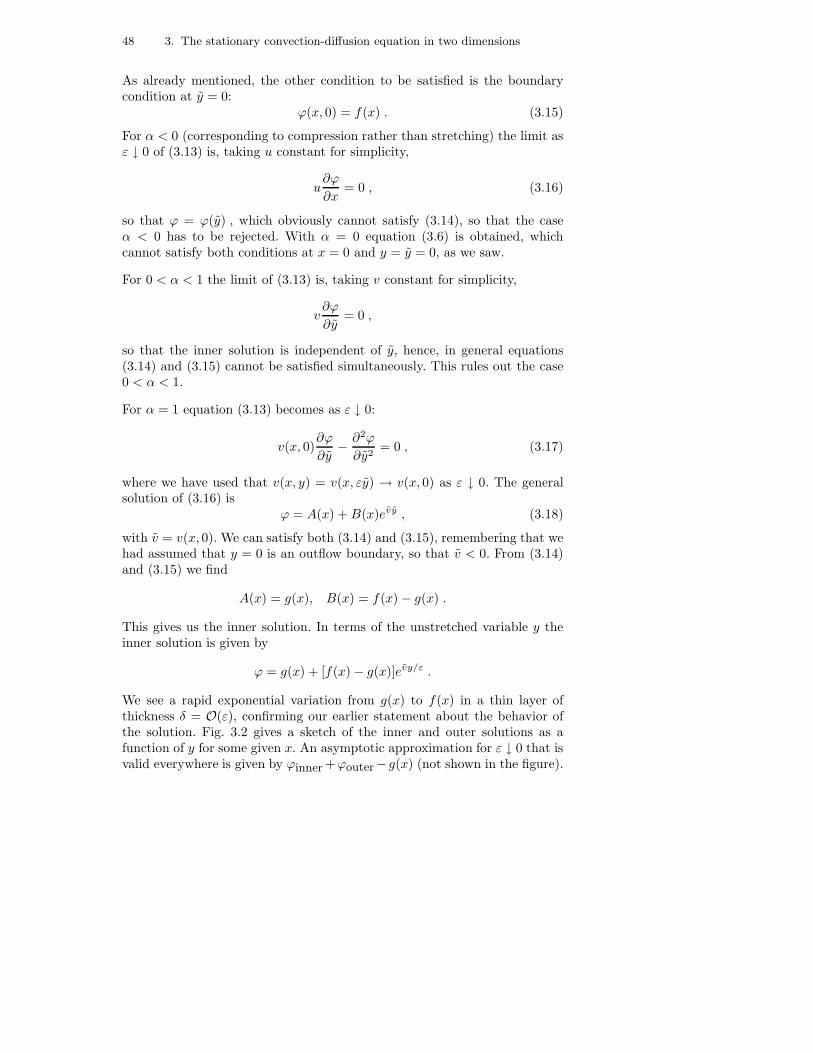
48 3. The stationary convection-diffusion equation in two dimensions
As already mentioned, the other condition to be satisfied is the boundarycondition at y = 0:
ϕ(x, 0) = f(x) . (3.15)
For α < 0 (corresponding to compression rather than stretching) the limit asε ↓ 0 of (3.13) is, taking u constant for simplicity,
u∂ϕ
∂x= 0 , (3.16)
so that ϕ = ϕ(y) , which obviously cannot satisfy (3.14), so that the caseα < 0 has to be rejected. With α = 0 equation (3.6) is obtained, whichcannot satisfy both conditions at x = 0 and y = y = 0, as we saw.
For 0 < α < 1 the limit of (3.13) is, taking v constant for simplicity,
v∂ϕ
∂y= 0 ,
so that the inner solution is independent of y, hence, in general equations(3.14) and (3.15) cannot be satisfied simultaneously. This rules out the case0 < α < 1.
For α = 1 equation (3.13) becomes as ε ↓ 0:
v(x, 0)∂ϕ
∂y− ∂2ϕ
∂y2= 0 , (3.17)
where we have used that v(x, y) = v(x, εy) → v(x, 0) as ε ↓ 0. The generalsolution of (3.16) is
ϕ = A(x) +B(x)evy , (3.18)
with v = v(x, 0). We can satisfy both (3.14) and (3.15), remembering that wehad assumed that y = 0 is an outflow boundary, so that v < 0. From (3.14)and (3.15) we find
A(x) = g(x), B(x) = f(x) − g(x) .
This gives us the inner solution. In terms of the unstretched variable y theinner solution is given by
ϕ = g(x) + [f(x) − g(x)]evy/ε .
We see a rapid exponential variation from g(x) to f(x) in a thin layer ofthickness δ = O(ε), confirming our earlier statement about the behavior ofthe solution. Fig. 3.2 gives a sketch of the inner and outer solutions as afunction of y for some given x. An asymptotic approximation for ε ↓ 0 that isvalid everywhere is given by ϕinner +ϕouter− g(x) (not shown in the figure).
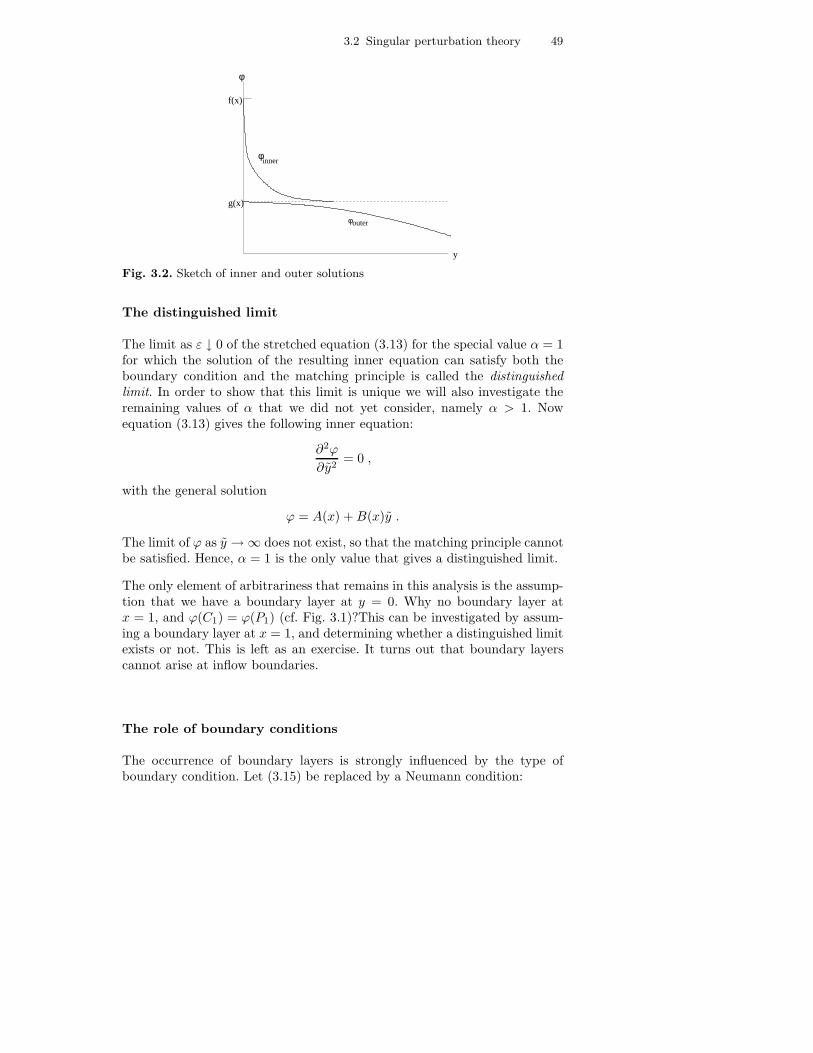
3.2 Singular perturbation theory 49
φinner
outerφ
f(x)
y
φ
g(x)
Fig. 3.2. Sketch of inner and outer solutions
The distinguished limit
The limit as ε ↓ 0 of the stretched equation (3.13) for the special value α = 1for which the solution of the resulting inner equation can satisfy both theboundary condition and the matching principle is called the distinguishedlimit. In order to show that this limit is unique we will also investigate theremaining values of α that we did not yet consider, namely α > 1. Nowequation (3.13) gives the following inner equation:
∂2ϕ
∂y2= 0 ,
with the general solution
ϕ = A(x) +B(x)y .
The limit of ϕ as y → ∞ does not exist, so that the matching principle cannotbe satisfied. Hence, α = 1 is the only value that gives a distinguished limit.
The only element of arbitrariness that remains in this analysis is the assump-tion that we have a boundary layer at y = 0. Why no boundary layer atx = 1, and ϕ(C1) = ϕ(P1) (cf. Fig. 3.1)?This can be investigated by assum-ing a boundary layer at x = 1, and determining whether a distinguished limitexists or not. This is left as an exercise. It turns out that boundary layerscannot arise at inflow boundaries.
The role of boundary conditions
The occurrence of boundary layers is strongly influenced by the type ofboundary condition. Let (3.15) be replaced by a Neumann condition:

50 3. The stationary convection-diffusion equation in two dimensions
−∂ϕ(x, 0)
∂y= f(x) . (3.19)
As before, a boundary layer of thickness O(ε) is found at y = 0, and theboundary layer equation is given by (3.16), with general solution (3.18). Tak-ing boundary condition (3.19) into account we find
B(x) = −εf(x)/v ,
so that B(x) → 0 as ε ↓ 0. Hence, to first order, there is no boundary layer,and the outer solution (solution of (3.6)) is uniformly valid in Ω.
Parabolic and ordinary boundary layers
Those familiar with fluid dynamics may wonder at the boundary layer thick-ness O(ε) = O(1/Pe), since in fluid dynamics laminar boundary layers havethickness O(1/
√Re), so that one would have expected δ = O(1/
√Pe). We
will now see that the convection-diffusion equation gives rise to two types ofboundary layers.
Consider the case that y = 0 is a solid wall, so that v(x, 0) = 0. The shape ofthe characteristics of the outer equation (3.6) might be as in Fig. 3.3, wherealso y = 1 is assumed to be a solid wall, so that we have a channel flow. Since
x
y
1
1
Fig. 3.3. Characteristics of equation (3.6) in a channel flow.
v(x, 0) = 0, the wall y = 0 is a characteristic of the outer equation (3.6)according to (3.7), so that the solution along this characteristic is given by
ϕ(x, 0) = f1(0) , (3.20)
assuming x = 0 is a inflow boundary with Dirichlet condition
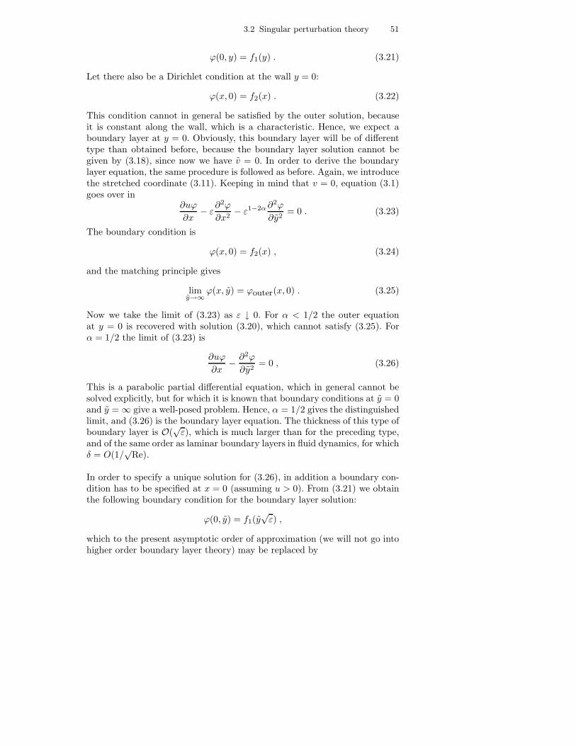
3.2 Singular perturbation theory 51
ϕ(0, y) = f1(y) . (3.21)
Let there also be a Dirichlet condition at the wall y = 0:
ϕ(x, 0) = f2(x) . (3.22)
This condition cannot in general be satisfied by the outer solution, becauseit is constant along the wall, which is a characteristic. Hence, we expect aboundary layer at y = 0. Obviously, this boundary layer will be of differenttype than obtained before, because the boundary layer solution cannot begiven by (3.18), since now we have v = 0. In order to derive the boundarylayer equation, the same procedure is followed as before. Again, we introducethe stretched coordinate (3.11). Keeping in mind that v = 0, equation (3.1)goes over in
∂uϕ
∂x− ε
∂2ϕ
∂x2− ε1−2α ∂
2ϕ
∂y2= 0 . (3.23)
The boundary condition is
ϕ(x, 0) = f2(x) , (3.24)
and the matching principle gives
limy→∞
ϕ(x, y) = ϕouter(x, 0) . (3.25)
Now we take the limit of (3.23) as ε ↓ 0. For α < 1/2 the outer equationat y = 0 is recovered with solution (3.20), which cannot satisfy (3.25). Forα = 1/2 the limit of (3.23) is
∂uϕ
∂x− ∂2ϕ
∂y2= 0 , (3.26)
This is a parabolic partial differential equation, which in general cannot besolved explicitly, but for which it is known that boundary conditions at y = 0and y = ∞ give a well-posed problem. Hence, α = 1/2 gives the distinguishedlimit, and (3.26) is the boundary layer equation. The thickness of this type ofboundary layer is O(
√ε), which is much larger than for the preceding type,
and of the same order as laminar boundary layers in fluid dynamics, for whichδ = O(1/
√Re).
In order to specify a unique solution for (3.26), in addition a boundary con-dition has to be specified at x = 0 (assuming u > 0). From (3.21) we obtainthe following boundary condition for the boundary layer solution:
ϕ(0, y) = f1(y√ε) ,
which to the present asymptotic order of approximation (we will not go intohigher order boundary layer theory) may be replaced by
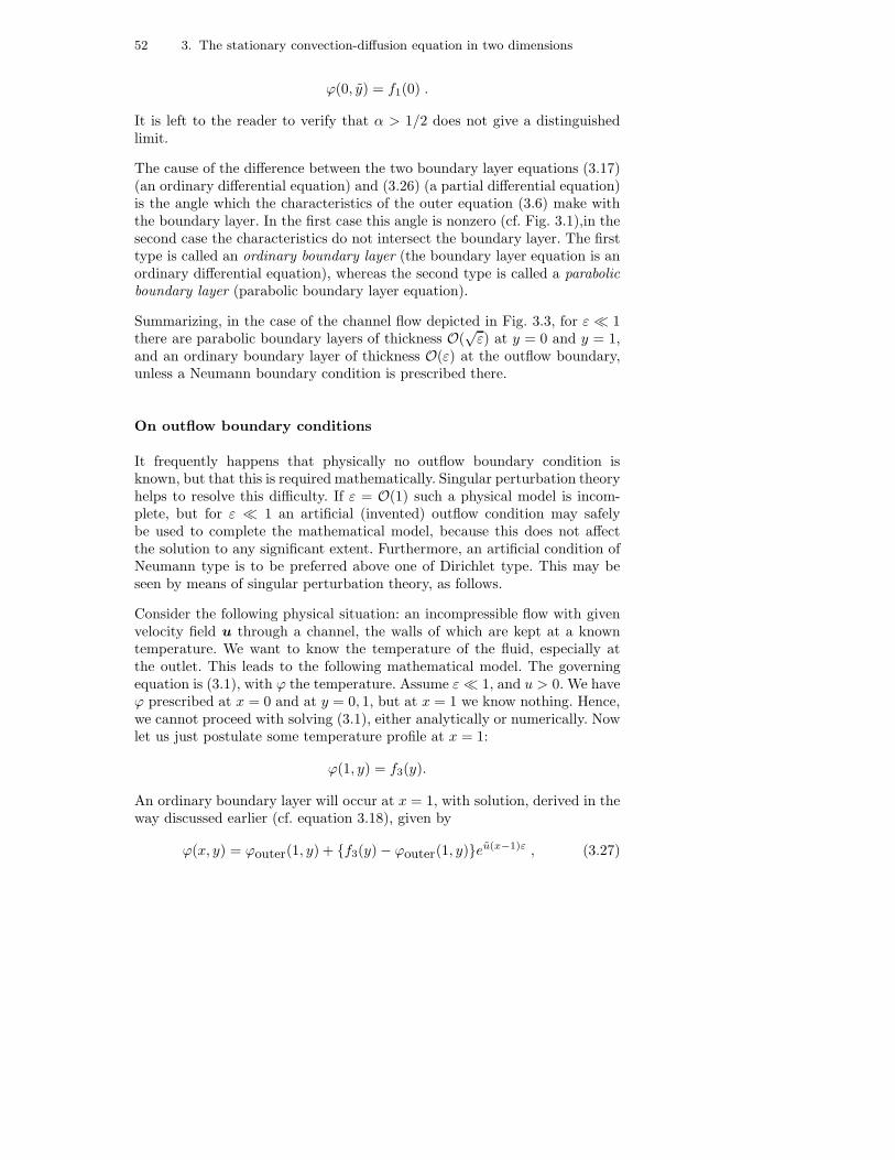
52 3. The stationary convection-diffusion equation in two dimensions
ϕ(0, y) = f1(0) .
It is left to the reader to verify that α > 1/2 does not give a distinguishedlimit.
The cause of the difference between the two boundary layer equations (3.17)(an ordinary differential equation) and (3.26) (a partial differential equation)is the angle which the characteristics of the outer equation (3.6) make withthe boundary layer. In the first case this angle is nonzero (cf. Fig. 3.1),in thesecond case the characteristics do not intersect the boundary layer. The firsttype is called an ordinary boundary layer (the boundary layer equation is anordinary differential equation), whereas the second type is called a parabolicboundary layer (parabolic boundary layer equation).
Summarizing, in the case of the channel flow depicted in Fig. 3.3, for ε ≪ 1there are parabolic boundary layers of thickness O(
√ε) at y = 0 and y = 1,
and an ordinary boundary layer of thickness O(ε) at the outflow boundary,unless a Neumann boundary condition is prescribed there.
On outflow boundary conditions
It frequently happens that physically no outflow boundary condition isknown, but that this is required mathematically. Singular perturbation theoryhelps to resolve this difficulty. If ε = O(1) such a physical model is incom-plete, but for ε ≪ 1 an artificial (invented) outflow condition may safelybe used to complete the mathematical model, because this does not affectthe solution to any significant extent. Furthermore, an artificial condition ofNeumann type is to be preferred above one of Dirichlet type. This may beseen by means of singular perturbation theory, as follows.
Consider the following physical situation: an incompressible flow with givenvelocity field u through a channel, the walls of which are kept at a knowntemperature. We want to know the temperature of the fluid, especially atthe outlet. This leads to the following mathematical model. The governingequation is (3.1), with ϕ the temperature. Assume ε≪ 1, and u > 0. We haveϕ prescribed at x = 0 and at y = 0, 1, but at x = 1 we know nothing. Hence,we cannot proceed with solving (3.1), either analytically or numerically. Nowlet us just postulate some temperature profile at x = 1:
ϕ(1, y) = f3(y).
An ordinary boundary layer will occur at x = 1, with solution, derived in theway discussed earlier (cf. equation 3.18), given by
ϕ(x, y) = ϕouter(1, y) + f3(y) − ϕouter(1, y)eu(x−1)ε , (3.27)
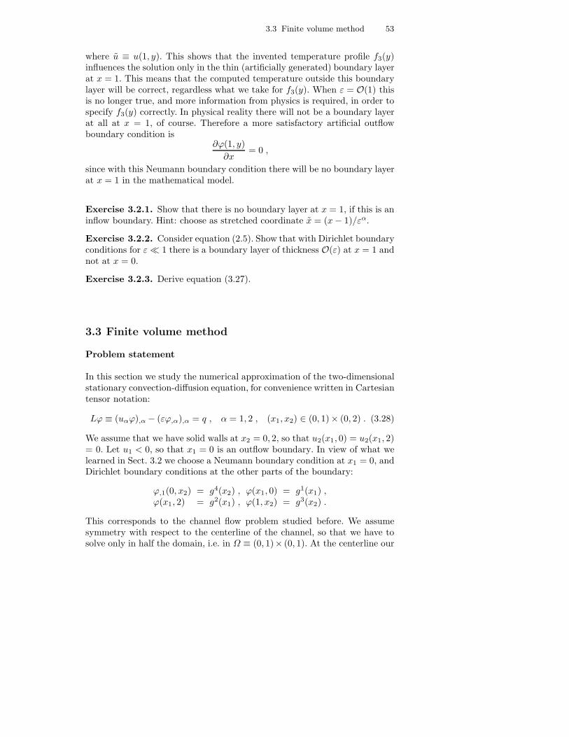
3.3 Finite volume method 53
where u ≡ u(1, y). This shows that the invented temperature profile f3(y)influences the solution only in the thin (artificially generated) boundary layerat x = 1. This means that the computed temperature outside this boundarylayer will be correct, regardless what we take for f3(y). When ε = O(1) thisis no longer true, and more information from physics is required, in order tospecify f3(y) correctly. In physical reality there will not be a boundary layerat all at x = 1, of course. Therefore a more satisfactory artificial outflowboundary condition is
∂ϕ(1, y)
∂x= 0 ,
since with this Neumann boundary condition there will be no boundary layerat x = 1 in the mathematical model.
Exercise 3.2.1. Show that there is no boundary layer at x = 1, if this is aninflow boundary. Hint: choose as stretched coordinate x = (x− 1)/εα.
Exercise 3.2.2. Consider equation (2.5). Show that with Dirichlet boundaryconditions for ε≪ 1 there is a boundary layer of thickness O(ε) at x = 1 andnot at x = 0.
Exercise 3.2.3. Derive equation (3.27).
3.3 Finite volume method
Problem statement
In this section we study the numerical approximation of the two-dimensionalstationary convection-diffusion equation, for convenience written in Cartesiantensor notation:
Lϕ ≡ (uαϕ),α − (εϕ,α),α = q , α = 1, 2 , (x1, x2) ∈ (0, 1)× (0, 2) . (3.28)
We assume that we have solid walls at x2 = 0, 2, so that u2(x1, 0) = u2(x1, 2)= 0. Let u1 < 0, so that x1 = 0 is an outflow boundary. In view of what welearned in Sect. 3.2 we choose a Neumann boundary condition at x1 = 0, andDirichlet boundary conditions at the other parts of the boundary:
ϕ,1(0, x2) = g4(x2) , ϕ(x1, 0) = g1(x1) ,ϕ(x1, 2) = g2(x1) , ϕ(1, x2) = g3(x2) .
This corresponds to the channel flow problem studied before. We assumesymmetry with respect to the centerline of the channel, so that we have tosolve only in half the domain, i.e. in Ω ≡ (0, 1)× (0, 1). At the centerline our
54 3. The stationary convection-diffusion equation in two dimensions
boundary condition is the symmetry condition ϕ,2 = 0, so that the boundaryconditions are:
ϕ,1(0, x2) = g4(x2) , ϕ(x1, 0) = g1(x1) ,ϕ,2(x1, 1) = 0 , ϕ(1, x2) = g3(x2) .
(3.29)
As discussed before, it is best to choose at the outflow boundary a homo-geneous Neumann condition, i.e. g4 ≡ 0, but for the purpose of numericalexperimentation we leave the possibility of choosing a nonhomogeneous Neu-mann condition open. We will not discuss the three-dimensional case, becausethis does not provide new insights.
Our purpose in this section is to show, as in Sect. 2.3, but this time in twodimensions, that (3.28) can be solved numerically such that accuracy andcomputing cost are uniform in Pe. Therefore fear that it is impossible tocompute high Peclet (Reynolds) number flow accurately is unfounded, as ar-gued before. For simplicity we assume horizontal flow: u2 ≡ 0, and we willsimply write u instead of u1.
Choice of grid
In view of what we learned in Sect. 3.2, we expect a parabolic (becauseu2 = 0) boundary layer at x2 = 0 with thickness O(
√ε). If g4 ≡ 0 we have a
homogeneous Neumann condition at the outflow boundary, and there is noboundary layer at x1 = 0. Just as in Sect. 2.3, in order to make accuracy andcomputing work uniform in ε, we choose a grid with local refinement in theboundary layer, as sketched in Fig. 3.4. We will apply grid refinement near theoutflow boundary later. The region of refinement has thickness σ = O(
√ε).
The precise choice of σ will be discussed later, and is such that the boundarylayer falls inside the refinement region. The refined part of the grid is calledGf , the interface between the refined and unrefined parts is called Γ and theremainder of the grid is called Gc. The mesh sizes in Gf and Gc are uniform,as indicated in Fig. 3.4. Note that the location of the horizontal grid linesdepends on ε.
Finite volume discretization
We choose a cell-centered scheme. The cell centers are labeled by integer two-tuples (i, j) in the usual way: Ωij is the cell with center at (xi, yj). Hence, forexample, (i+ 1/2, j) refers to the center of a vertical cell edge. Cell-centeredfinite volume discretization is used as described in Sect. 2.3. For completenessthe discretization is summarized below. The finite volume method gives byintegration over Ωij and by using the divergence theorem:

3.3 Finite volume method 55
Γ
G
H
H
2
c
fG
1h
σ
2
Fig. 3.4. Computational grid
∫
Ωij
LϕdΩ =[
∫ xi+1/2,j+1/2
xi+1/2,j−1/2−
∫ xi−1/2,j+1/2
xi−1/2,j−1/2
]
(uϕ− εϕ,1)dx2
+[
∫ xi+1/2,j+1/2
xi−1/2,j+1/2−
∫ xi+1/2,j−1/2
xi−1/2,j−1/2
]
(−εϕ,2)dx1
= F 1|i+1/2,ji−1/2,j + F 2|i,j+1/2
i,j−1/2 .
The approximation of the numerical fluxes F 1,2 is given below. The right-hand side of equation (3.28) is numerically integrated over Ωij as follows:
∫
Ωij
qdΩ ∼= qij ≡ H1Kjq(xij) , (3.30)
where Kj is the vertical dimension of Ωij : Kj = h2 in Gf and Kj = H2
in Gc. The cells are numbered i = 1, ..., I and j = 1, ..., J in the x1- andx2-directions, respectively. The following scheme is obtained:
Lhϕij ≡ F 1|i+1/2,ji−1/2,j + F 2|i,j+1/2
i,j−1/2 = qij . (3.31)
If we sum (3.31) over all cells only boundary fluxes remain, so that the schemeis conservative (cf. Sect. 2.3).
The numerical flux
How to approximate the numerical fluxes F 1,2 in terms of neighboring gridfunction values follows directly from the one-dimensional case discussed inthe preceding chapter. With upwind discretization for the first derivative(taking into account that u < 0), the numerical fluxes F 1,2 are approximatedas follows:

56 3. The stationary convection-diffusion equation in two dimensions
F 1i+1/2,j
∼= Kj[ui+1/2,jϕi+1,j − ε(ϕi+1,j − ϕij)/H1] ,
F 2i,j+1/2
∼= −2H1ε(ϕi,j+1 − ϕij)/(Kj +Kj+1) , (3.32)
With the central scheme for the first derivative F 1 becomes:
F 1i+1/2,j
∼= Kj[ui+1/2,j(ϕi,j + ϕi+1,j)/2 − ε(ϕi+1,j − ϕij)/H1] . (3.33)
The boundary conditions are implemented as in Sect. 2.3. This gives bothfor the upwind and central schemes:
F 11/2,j
∼= Kj [u1/2,j(ϕ1j −H1g4(yj)/2) − εg4(yj)] ,
F 1I+1/2,j
∼= Kj [uI+1/2,jϕI+1/2,j − 2ε(ϕI+1/2,j − ϕIj)/H1] ,
F 2i,1/2
∼= −2H1ε(ϕi,1 − ϕi,1/2)/h2 ,
F 2i,J+1/2 = 0 ,
(3.34)
where ϕI+1/2,j and ϕi,1/2 are given by the boundary conditions (3.29).
The stencil of the scheme
Although this is tedious, we will spell out more details of the scheme, aspreparation for a MATLAB program. The numerical fluxes as specified abovecan be written as
F 1i+1/2,j = β0
ijϕij + β1i+1,jϕi+1,j , i = 1, · · · , I − 1 , j = 1, · · · , J ,
F 11/2,j = β1
1jϕ1,j + γ0j , j = 1, · · · , J ,
F 1I+1/2,j = β0
IjϕIj + γ1j , j = 1, · · · , J ,
F 2i,j+1/2 = β2
ijϕij + β3i,j+1ϕi,j+1, i = 1, · · · , I , j = 1, · · · , J − 1 ,
F 2i,1/2 = β3
i1ϕi,1 + γ2i , i = 1, · · · , I ,
F 2i,J+1/2 = 0 , i = 1, · · · , I ,
(3.35)
where γ0, γ1, γ2 are known terms arising from the boundary conditions. Theβ and γ coefficients follow easily from (3.34), and will not be written down.The scheme consists of a linear system of equations of the form
Lhϕij =1
∑
k=−1
1∑
l=−1
αklijϕi+k,j+l , (3.36)
where the only nonzero α coefficients are
α−1,0ij = −β0
i−1,j , α1,0ij = β1
ij
α0,−1ij = −β2
i,j−1 , α0,1ij = β3
ij
α0,0ij = (β0 − β1 + β2 − β3)ij .
(3.37)
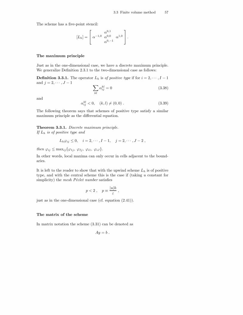
3.3 Finite volume method 57
The scheme has a five-point stencil:
[Lh] =
α0,1
α−1,0 α0,0 α1,0
α0,−1
.
The maximum principle
Just as in the one-dimensional case, we have a discrete maximum principle.We generalize Definition 2.3.1 to the two-dimensional case as follows:
Definition 3.3.1. The operator Lh is of positive type if for i = 2, · · · , I − 1and j = 2, · · · , J − 1
∑
kl
αklij = 0 (3.38)
andαkl
ij < 0, (k, l) 6= (0, 0) . (3.39)
The following theorem says that schemes of positive type satisfy a similarmaximum principle as the differential equation.
Theorem 3.3.1. Discrete maximum principle.If Lh is of positive type and
Lhϕij ≤ 0, i = 2, · · · , I − 1, j = 2, · · · , J − 2 ,
then ϕij ≤ maxijϕ1j , ϕIj , ϕi1, ϕiJ.In other words, local maxima can only occur in cells adjacent to the bound-aries.
It is left to the reader to show that with the upwind scheme Lh is of positivetype, and with the central scheme this is the case if (taking u constant forsimplicity) the mesh Peclet number satisfies
p < 2 , p ≡ |u|hε
,
just as in the one-dimensional case (cf. equation (2.41)).
The matrix of the scheme
In matrix notation the scheme (3.31) can be denoted as
Ay = b .
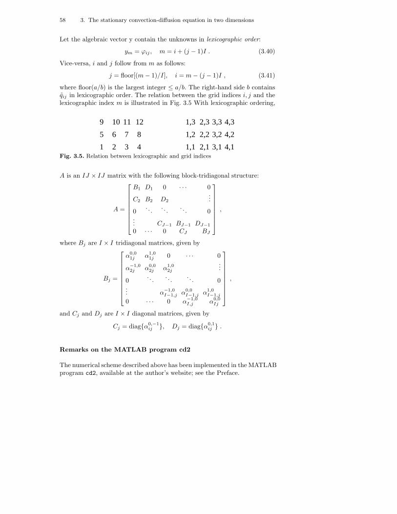
58 3. The stationary convection-diffusion equation in two dimensions
Let the algebraic vector y contain the unknowns in lexicographic order:
ym = ϕij , m = i+ (j − 1)I . (3.40)
Vice-versa, i and j follow from m as follows:
j = floor[(m− 1)/I], i = m− (j − 1)I , (3.41)
where floor(a/b) is the largest integer ≤ a/b. The right-hand side b containsqij in lexicographic order. The relation between the grid indices i, j and thelexicographic index m is illustrated in Fig. 3.5 With lexicographic ordering,
1 2 3 4
5 6 7 8
1,1 2,1 3,1 4,1
1,2 2,2 3,2 4,2
9 10 11 12 1,3 2,3 3,3 4,3
Fig. 3.5. Relation between lexicographic and grid indices
A is an IJ × IJ matrix with the following block-tridiagonal structure:
A =
B1 D1 0 · · · 0
C2 B2 D2
...
0. . .
. . .. . . 0
... CJ−1 BJ−1 DJ−1
0 · · · 0 CJ BJ
,
where Bj are I × I tridiagonal matrices, given by
Bj =
α0,01j α1,0
1j 0 · · · 0
α−1,02j α0,0
2j α1,02j
...
0. . .
. . .. . . 0
... α−1,0I−1,j α0,0
I−1,j α1,0I−1,j
0 · · · 0 α−1,0I,j α0,0
Ij
,
and Cj and Dj are I × I diagonal matrices, given by
Cj = diagα0,−1ij , Dj = diagα0,1
ij .
Remarks on the MATLAB program cd2
The numerical scheme described above has been implemented in the MATLABprogram cd2, available at the author’s website; see the Preface.

3.3 Finite volume method 59
The student is not expected to fully understand this program, because useis made of somewhat advanced features, such as meshgrid and reshape, inorder to avoid for loops. Avoiding for loops is essential for efficiency inMATLAB, as can be seen in the code cd2 by comparing computing time(using tic· · ·toc) for generating the matrices A1 and A3. Generation of A1is done in a simple way with for loops, and requires 1.22 time units on a32×72 grid, whereas the more sophisticated program for A3 takes 0.067 timeunits; this discrepancy grows rapidly with increasing grid size. The time usedfor solving the system Ay = b is 0.32.
In MATLAB, A is generated as a sparse matrix by
d = [-I; -1; 0; 1; I];
A = spdiags([a1 a2 -a1-a2-a4-a5 a4 a5], d, n, n);
with suitable definition of the diagonals a1· · ·a5. Exploiting sparsity is es-sential for saving memory and computing time. The solution of the systemAy = b is obtained in MATLAB by
y = A\b;
This means that we solve with a direct method using sparse LU factorization.For large systems, that occur particularly when partial differential equationsare solved in three-dimensional domains, direct methods frequently demandintolerable amounts of computer time and memory, even when sparsity isexploited. Efficient solution methods for solving the algebraic systems arisingfrom numerical schemes for partial differential equations will be discussed inChapt. 6.
Numerical experiments
The purpose of the numerical experiments with the program cd2 that we willnow describe is to demonstrate, as we did in Sect. 2.3 for the one-dimensionalcase, that we can achieve Peclet-uniform accuracy and efficiency, and thataccurate results can be obtained on grids with large jumps in mesh size. Thisis shown theoretically in Sect. 4.7 of Wesseling (2001), but here we confineourselves to numerical illustration.
In order to be able to assess the error, we choose an exact solution. Of course,this solution has to exhibit the boundary layer behavior occurring in prac-tice. We choose the following solution of the boundary layer (inner) equation(3.26):
ϕ =1√
2 − x
exp(− y2
4ε(2 − x)) + exp(− (2 − y)2
4ε(2 − x)
.
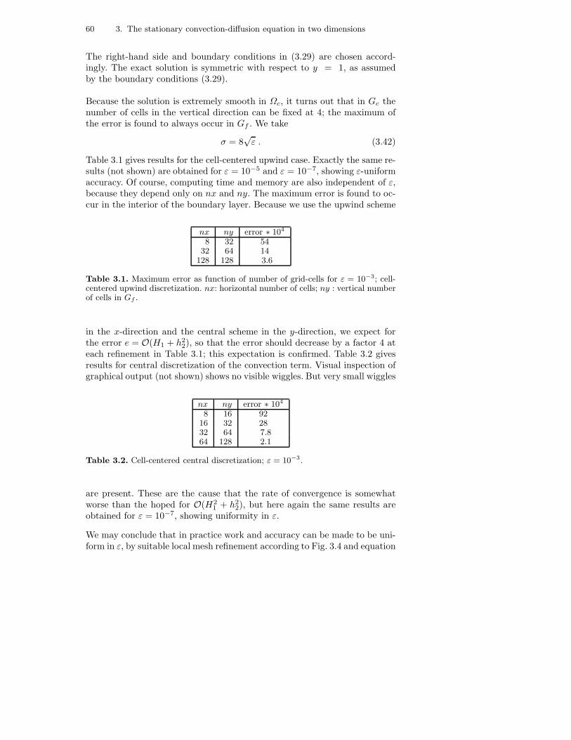
60 3. The stationary convection-diffusion equation in two dimensions
The right-hand side and boundary conditions in (3.29) are chosen accord-ingly. The exact solution is symmetric with respect to y = 1, as assumedby the boundary conditions (3.29).
Because the solution is extremely smooth in Ωc, it turns out that in Gc thenumber of cells in the vertical direction can be fixed at 4; the maximum ofthe error is found to always occur in Gf . We take
σ = 8√ε . (3.42)
Table 3.1 gives results for the cell-centered upwind case. Exactly the same re-sults (not shown) are obtained for ε = 10−5 and ε = 10−7, showing ε-uniformaccuracy. Of course, computing time and memory are also independent of ε,because they depend only on nx and ny. The maximum error is found to oc-cur in the interior of the boundary layer. Because we use the upwind scheme
nx ny error ∗ 104
8 32 5432 64 14
128 128 3.6
Table 3.1. Maximum error as function of number of grid-cells for ε = 10−3; cell-centered upwind discretization. nx: horizontal number of cells; ny : vertical numberof cells in Gf .
in the x-direction and the central scheme in the y-direction, we expect forthe error e = O(H1 + h2
2), so that the error should decrease by a factor 4 ateach refinement in Table 3.1; this expectation is confirmed. Table 3.2 givesresults for central discretization of the convection term. Visual inspection ofgraphical output (not shown) shows no visible wiggles. But very small wiggles
nx ny error ∗ 104
8 16 9216 32 2832 64 7.864 128 2.1
Table 3.2. Cell-centered central discretization; ε = 10−3.
are present. These are the cause that the rate of convergence is somewhatworse than the hoped for O(H2
1 + h22), but here again the same results are
obtained for ε = 10−7, showing uniformity in ε.
We may conclude that in practice work and accuracy can be made to be uni-form in ε, by suitable local mesh refinement according to Fig. 3.4 and equation
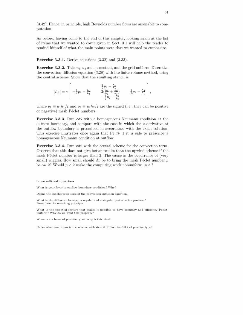
61
(3.42). Hence, in principle, high Reynolds number flows are amenable to com-putation.
As before, having come to the end of this chapter, looking again at the listof items that we wanted to cover given in Sect. 3.1 will help the reader toremind himself of what the main points were that we wanted to emphasize.
Exercise 3.3.1. Derive equations (3.32) and (3.33).
Exercise 3.3.2. Take u1, u2 and ε constant, and the grid uniform. Discretizethe convection-diffusion equation (3.28) with hte finite volume method, usingthe central scheme. Show that the resulting stancil is
[Lh] = ε
12p2 − h1
h2
− 12p1 − h2
h12(h1
h2+ h2
h1) 1
2p1 − h2
h1
− 12p2 − h1
h2
,
where p1 ≡ u1h1/ε and p2 ≡ u2h2/ε are the signed (i.e., they can be positiveor negative) mesh Peclet numbers.
Exercise 3.3.3. Run cd2 with a homogeneous Neumann condition at theoutflow boundary, and compare with the case in which the x-derivative atthe outflow boundary is prescribed in accordance with the exact solution.This exercise illustrates once again that Pe ≫ 1 it is safe to prescribe ahomogeneous Neumann condition at outflow.
Exercise 3.3.4. Run cd2 with the central scheme for the convection term.Observe that this does not give better results than the upwind scheme if themesh Peclet number is larger than 2. The cause is the occurrence of (verysmall) wiggles. How small should dx be to bring the mesh Peclet number pbelow 2? Would p < 2 make the computing work nonuniform in ε ?
Some self-test questions
What is your favorite outflow boundary condition? Why?
Define the subcharacteristics of the convection-diffusion equation.
What is the difference between a regular and a singular perturbation problem?Formulate the matching principle.
What is the essential feature that makes it possible to have accuracy and efficiency Peclet-uniform? Why do we want this property?
When is a scheme of positive type? Why is this nice?
Under what conditions is the scheme with stencil of Exercise 3.3.2 of positive type?

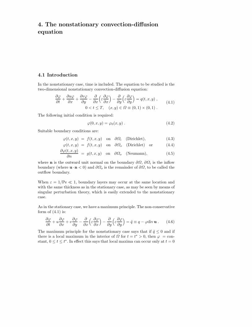
4. The nonstationary convection-diffusion
equation
4.1 Introduction
In the nonstationary case, time is included. The equation to be studied is thetwo-dimensional nonstationary convection-diffusion equation:
∂ϕ
∂t+∂uϕ
∂x+∂vϕ
∂y− ∂
∂x
(
ε∂ϕ
∂x
)
− ∂
∂y
(
ε∂ϕ
∂y
)
= q(t, x, y) ,
0 < t ≤ T, (x, y) ∈ Ω ≡ (0, 1)× (0, 1) .
(4.1)
The following initial condition is required:
ϕ(0, x, y) = ϕ0(x, y) . (4.2)
Suitable boundary conditions are:
ϕ(t, x, y) = f(t, x, y) on ∂Ωi (Dirichlet), (4.3)
ϕ(t, x, y) = f(t, x, y) on ∂Ωo (Dirichlet) or (4.4)
∂ϕ(t, x, y)
∂n= g(t, x, y) on ∂Ωo (Neumann), (4.5)
where n is the outward unit normal on the boundary ∂Ω, ∂Ωi is the inflowboundary (where u ·n < 0) and ∂Ωo is the remainder of ∂Ω, to be called theoutflow boundary.
When ε = 1/Pe ≪ 1, boundary layers may occur at the same location andwith the same thickness as in the stationary case, as may be seen by means ofsingular perturbation theory, which is easily extended to the nonstationarycase.
As in the stationary case, we have a maximum principle. The non-conservativeform of (4.1) is:
∂ϕ
∂t+ u
∂ϕ
∂x+ v
∂ϕ
∂y− ∂
∂x
(
ε∂ϕ
∂x
)
− ∂
∂y
(
ε∂ϕ
∂y
)
= q ≡ q − ϕdivu . (4.6)
The maximum principle for the nonstationary case says that if q ≤ 0 and ifthere is a local maximum in the interior of Ω for t = t∗ > 0, then ϕ = con-stant, 0 ≤ t ≤ t∗. In effect this says that local maxima can occur only at t = 0
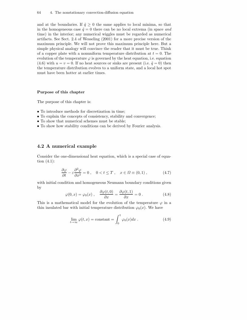
64 4. The nonstationary convection-diffusion equation
and at the boundaries. If q ≥ 0 the same applies to local minima, so thatin the homogeneous case q = 0 there can be no local extrema (in space andtime) in the interior; any numerical wiggles must be regarded as numericalartifacts. See Sect. 2.4 of Wesseling (2001) for a more precise version of themaximum principle. We will not prove this maximum principle here. But asimple physical analogy will convince the reader that it must be true. Thinkof a copper plate with a nonuniform temperature distribution at t = 0. Theevolution of the temperature ϕ is governed by the heat equation, i.e. equation(4.6) with u = v = 0. If no heat sources or sinks are present (i.e. q = 0) thenthe temperature distribution evolves to a uniform state, and a local hot spotmust have been hotter at earlier times.
Purpose of this chapter
The purpose of this chapter is:
• To introduce methods for discretization in time;• To explain the concepts of consistency, stability and convergence;• To show that numerical schemes must be stable;• To show how stability conditions can be derived by Fourier analysis.
4.2 A numerical example
Consider the one-dimensional heat equation, which is a special case of equa-tion (4.1):
∂ϕ
∂t− ε
∂2ϕ
∂x2= 0 , 0 < t ≤ T , x ∈ Ω ≡ (0, 1) , (4.7)
with initial condition and homogeneous Neumann boundary conditions givenby
ϕ(0, x) = ϕ0(x) ,∂ϕ(t, 0)
∂x=∂ϕ(t, 1)
∂x= 0 . (4.8)
This is a mathematical model for the evolution of the temperature ϕ in athin insulated bar with initial temperature distribution ϕ0(x). We have
limt→∞
ϕ(t, x) = constant =
∫ 1
0
ϕ0(x)dx . (4.9)

4.2 A numerical example 65
Discretization in space
For discretization in space we use the finite volume method on the vertex-centered grid of Fig. 2.1 with uniform mesh size h. The following details havebeen covered in the preceding chapters, but we present them as an exercise.Integration over the control volumes gives, with ε constant:
h
2
dϕ1
dt+ F1/2 − F3/2 = 0 ,
hdϕj
dt+ Fj−1/2 − Fj+1/2 = 0 , j = 2, · · · , J − 1 ,
h
2
dϕJ
dt+ FJ−1/2 − FJ+1/2 = 0 ,
(4.10)
where F is an approximation of ε∂ϕ/∂x, naturally chosen as follows:
Fj+1/2 = ε(ϕj+1 − ϕj)/h , j = 1, · · · , J − 1 .
From the boundary conditions it follows that F1/2 = FJ+1/2 = 0.
Discretization in time
Equation (4.10) is rewritten as
dϕj
dt+ Lhϕj = 0 , j = 1, · · · , J . (4.11)
For discretization in time we choose the forward Euler scheme:
(ϕn+1j − ϕn
j )/τ + Lhϕnj = 0 , n = 0, · · · , N , N ≡ T/τ , (4.12)
with τ the time step, taken constant; ϕnj is the numerical approximation
of ϕ(nτ, xj) with ϕ(t, x) the exact solution. From Fig. 2.1 it follows thatxj = (j − 1)h, h = 1/(J − 1). Equation (4.12) is equivalent to
ϕn+11 = (1 − 2d)ϕn
1 + 2dϕn2 ,
ϕn+1j = dϕn
j−1 + (1 − 2d)ϕnj + dϕn
j+1 , j = 2, · · · , J − 1 ,
ϕn+1J = 2dϕn
J−1 + (1 − 2d)ϕnJ ,
(4.13)
where d ≡ ετ/h2 is a dimensionless number, that we will call the diffusionnumber.
The matrix of the scheme
If we define ϕ≡ (ϕ1, · · · , ϕJ )T then (4.13) can be rewritten as
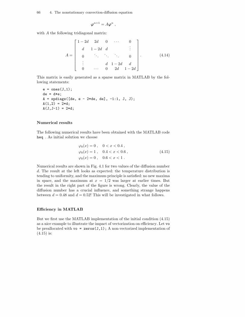
66 4. The nonstationary convection-diffusion equation
ϕn+1 = Aϕn ,
with A the following tridiagonal matrix:
A =
1 − 2d 2d 0 · · · 0
d 1 − 2d d...
0. . .
. . .. . . 0
... d 1 − 2d d0 · · · 0 2d 1 − 2d
. (4.14)
This matrix is easily generated as a sparse matrix in MATLAB by the fol-lowing statements:
e = ones(J,1);
de = d*e;
A = spdiags([de, e - 2*de, de], -1:1, J, J);
A(1,2) = 2*d;
A(J,J-1) = 2*d;
Numerical results
The following numerical results have been obtained with the MATLAB codeheq . As initial solution we choose
ϕ0(x) = 0 , 0 < x < 0.4 ,
ϕ0(x) = 1 , 0.4 < x < 0.6 ,
ϕ0(x) = 0 , 0.6 < x < 1 .
(4.15)
Numerical results are shown in Fig. 4.1 for two values of the diffusion numberd. The result at the left looks as expected: the temperature distribution istending to uniformity, and the maximum principle is satisfied: no new maximain space, and the maximum at x = 1/2 was larger at earlier times. Butthe result in the right part of the figure is wrong. Clearly, the value of thediffusion number has a crucial influence, and something strange happensbetween d = 0.48 and d = 0.52! This will be investigated in what follows.
Efficiency in MATLAB
But we first use the MATLAB implementation of the initial condition (4.15)as a nice example to illustrate the impact of vectorization on efficiency. Let vobe preallocated with vo = zeros(J,1); A non-vectorized implementation of(4.15) is:
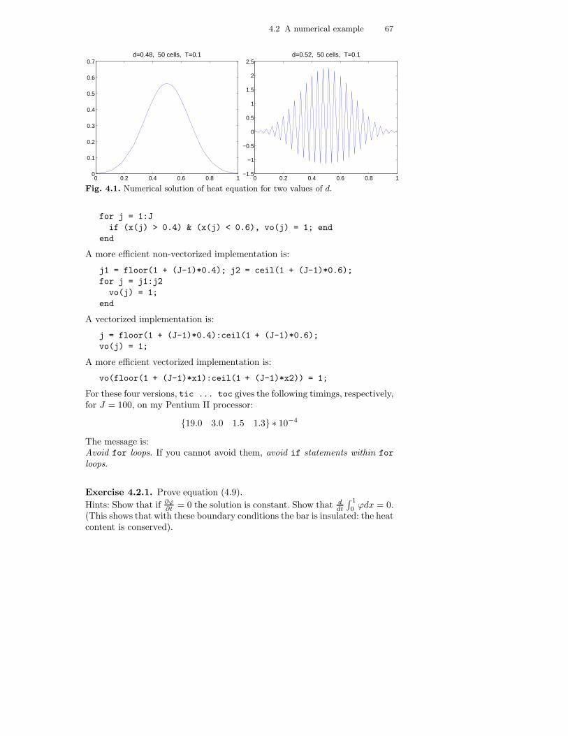
4.2 A numerical example 67
0 0.2 0.4 0.6 0.8 10
0.1
0.2
0.3
0.4
0.5
0.6
0.7d=0.48, 50 cells, T=0.1
0 0.2 0.4 0.6 0.8 1−1.5
−1
−0.5
0
0.5
1
1.5
2
2.5d=0.52, 50 cells, T=0.1
Fig. 4.1. Numerical solution of heat equation for two values of d.
for j = 1:J
if (x(j) > 0.4) & (x(j) < 0.6), vo(j) = 1; end
end
A more efficient non-vectorized implementation is:
j1 = floor(1 + (J-1)*0.4); j2 = ceil(1 + (J-1)*0.6);
for j = j1:j2
vo(j) = 1;
end
A vectorized implementation is:
j = floor(1 + (J-1)*0.4):ceil(1 + (J-1)*0.6);
vo(j) = 1;
A more efficient vectorized implementation is:
vo(floor(1 + (J-1)*x1):ceil(1 + (J-1)*x2)) = 1;
For these four versions, tic ... toc gives the following timings, respectively,for J = 100, on my Pentium II processor:
19.0 3.0 1.5 1.3 ∗ 10−4
The message is:Avoid for loops. If you cannot avoid them, avoid if statements within for
loops.
Exercise 4.2.1. Prove equation (4.9).
Hints: Show that if ∂ϕ∂t = 0 the solution is constant. Show that d
dt
∫ 1
0 ϕdx = 0.(This shows that with these boundary conditions the bar is insulated: the heatcontent is conserved).
68 4. The nonstationary convection-diffusion equation
4.3 Convergence, consistency and stability
One-step schemes
Schemes in which only two time levels are involved are called one-stepschemes; the forward Euler method (4.12) is an example. The general formof linear one-step schemes is:
B1ϕn+1 = B0ϕ
n +B2qn +B3q
n+1 , (4.16)
where B0, · · · , B3 are linear operators, and where q arises from the right-handside of the differential equation and the boundary conditions. For simplicitywe restrict ourselves here to one-step schemes.
Local and global truncation error
Let us denote the algebraic vector with elements the exact solution evaluatedat the grid point and at time tn by ϕn
e . Let us define the local truncationerror τn
j , gathered in an algebraic vector τn (not to be confused with thetime step τ) by the following equation:
B1ϕn+1e = B0ϕ
ne +B2q
n +B3qn+1 + τn . (4.17)
The global truncation error is defined as
en ≡ ϕne − ϕn . (4.18)
By subtracting (4.17) and (4.16) we get the following relation between theglobal and the local truncation error:
B1en+1 = B0e
n + τn . (4.19)
This is very similar to equation (2.47), so that the above definitions areconsistent with the truncation error definitions for the stationary case givenin Sect. 2.3.
Convergence
Of course, we want ‖en‖ ↓ 0, n = 1, · · · , T/τ as the grid is refined and τ ↓ 0(while keeping T/τ integer, obviously). This is not the case for our previousnumerical example when d > 1/2. No matter how small h and τ are chosen,the numerical solution will always look like the right part of Fig. 4.1, sinceit depends only on the parameter d, cf. (4.13). Clearly, we have to do someanalysis to find conditions that guarantee that a numerical scheme is good.

4.3 Convergence, consistency and stability 69
Let the number of space dimensions be m and let us have an m-dimensionalspatial grid G with grid points
xj = (x1j1 , · · · , xm
jm) .
Hence, now j is a multi-index (j1, · · · , jm). Let the spatial mesh sizes andthe time step be decreasing functions of a parameter h, that belongs to asequence that decreases to zero. To emphasize the dependence of G on h wewrite Gh. We want at a fixed time T and a fixed location x the error to tendto 0 as h ↓ 0. This implies that the number of time steps n = T/τ changes,and the multi-index j changes to keep xj fixed. To emphasize this we writejh. Of course, we assume that Gh is such that the fixed point xjh
remains agrid point when the grid is refined. For example, in the preceding numericalexample we could choose
xjh= 1/2 , h ∈ 1/2, 1/4, 1/6, · · · .
so that jh ∈ 1, 2, 3, · · · . We are now ready for the definition of convergence.
Definition 4.3.1. ConvergenceA scheme is called convergent if the global truncation error satisfies
limh↓0
eT/τjh
= 0, xjhfixed.
Clearly, scheme (4.13) is not convergent for d > 1/2.
Consistency
It seems likely that for convergence it is necessary that the local truncationerror is small enough. We therefore formulate a condition. Let the scheme(4.16) in a given grid point xj approximate the differential equation timesτα|∂Ωj |β with |∂Ωj | the volume of some cell around xj (For example, thescheme (4.13) obviously approximates equation (4.7) times τ , so that in thiscase α = 1, β = 0). We define
Definition 4.3.2. ConsistencyThe scheme (4.16) is called consistent if
limh↓0
τnjh/(τα|∂Ωjh
|β) = 0, j ∈ Gh, 1 ≤ n ≤ T/τ .
In Exercise 4.3.1 the reader is asked to show that scheme (2.48) is not consis-tent on rough grids. This seems disturbing, because we are going to show thatconsistency is necessary for convergence, but in Sect. 2.3 it was shown thatscheme (2.48) converges on rough grids. This apparent paradox arises fromthe fact that Def. 4.3.2 implies that the local truncation error is measured
70 4. The nonstationary convection-diffusion equation
in the maximum norm. On rough grids we have consistency of scheme (2.48)in a more sophisticated norm, but not in the maximum norm; we will not gointo this further. In this chapter only uniform grids are considered; on thesegrids the various appropriate norms are the same.
Stability
As illustrated by the numerical example in the preceding section, consistencydoes not imply convergence. In addition, stability is required. This conceptwill now be explained. Let δ0 be a hypothetical arbitrary perturbation ofϕ0. The resulting perturbation of ϕn is called δn. It is left for the reader toderive from equation (4.16) that
B1δn+1 = B0δ
n . (4.20)
Let ‖ · ‖h be some norm for functions Gh → R. Stability means that δn
remains bounded as n→ ∞, for all δ0. Two useful definitions are:
Definition 4.3.3. Zero-stabilityA scheme is called zero-stable if there exists a bounded function C(T ) and afunction τ0(h) such that for arbitrary δ0
‖δT/τ‖h ≤ C(T )‖δ0‖h (4.21)
for all τ ≤ τ0(h) and all h ≤ h0 for some fixed h0.
The appellation ”zero-stability” refers to the fact that the limit h ↓ 0 isconsidered.
Definition 4.3.4. Absolute stabilityA scheme is called absolutely stable if there exists a constant C and a functionτ0(h) such that for arbitrary δ0
‖δn‖h ≤ C‖δ0‖h (4.22)
for h fixed, all n > 0 and all τ ≤ τ0(h).
The difference with zero-stability is that here h is fixed.
Lax’s equivalence theorem
Definition 4.3.3 considers the perturbation at a fixed time T as h ↓ 0, whichis the same limit as in the definition of convergence. It can be shown thatconvergence implies zero-stability, and zero-stability plus consistency implyconvergence. This is known as Lax’s equivalence theorem. As a consequence,zero-stability is necessary for convergence. But absolute stability is also goodto have, because it allows n to grow indefinitely, making it possible to continuetime stepping until a steady state is reached. Absolute and zero-stability arenot completely equivalent.
4.4 Fourier stability analysis 71
A remark on stability analysis
The purpose of stability analysis is to find a suitable function τ0(h) such that(4.21) and (4.22) hold. This is the case if the linear operators in (4.20) satisfy
‖(B−11 B0)
n‖h ≤ C .
In the case of absolute stability, h and hence the dimensions of the matricesB0 and B1 are fixed, and linear algebra can be used to find conditions underwhich ‖(B−1
1 B0)n‖ is bounded as n → ∞. But in the case of zero-stability,
n→ ∞ and h ↓ 0 simultaneously, and we have to study not just the behaviorof the nth power of a matrix, but of a family of matrices of increasing size.This is not a familiar situation in linear algebra. We will see that Fourieranalysis is well-suited to the study of both kinds of stability, if the boundaryconditions are periodic.
Exercise 4.3.1. Show that for scheme(2.48) we have β = 1. Because thisscheme is for the stationary case, time can be disregarded. Show that, using(2.52), scheme (2.48) is consistent on smooth grids (as defined below equation(2.52)), but not on rough grids.
4.4 Fourier stability analysis
Applicability of Fourier analysis
In general it is difficult to derive estimates like (4.21) and (4.22). But if thecoefficients in the scheme are constant, the mesh uniform, the grid a rect-angular block and the boundary conditions periodic, then Fourier analysisapplies and the required estimates are often not difficult to obtain.
In practice, of course, the coefficients are usually not constant. The schemeis called locally stable if we have stability for the constant coefficients schemethat results from taking local values of the coefficients, and to assign thesevalues to the coefficients in the whole domain (frozen coefficients method).Local stability in the whole domain is necessary for stability in the variablecoefficients case. We will discuss stability only for constant coefficients.
Stability theory for non-periodic boundary conditions is complicated. Butfor explicit time stepping schemes it takes a while before the influence of theboundary conditions makes itself felt in the interior, so that Fourier stabilitytheory applies during a certain initial time span. As a consequence, stabilitywith periodic boundary conditions is desirable, even if the boundary condi-tions are of different type.

72 4. The nonstationary convection-diffusion equation
Example of frozen coefficients method
Consider the Burgers equation:
∂ϕ
∂t+
1
2
∂ϕ2
∂x= 0 .
Discretization with the forward Euler method in time and the upwind schemein space gives:
ϕn+1j − ϕn
j +τ
2h[(ϕn
j )2 − (ϕnj−1)
2] = 0 ,
assuming ϕ > 0 and a uniform grid. For stability analysis we postulate aperturbation δϕ0 of the initial solution. The perturbed solution satisfies
(ϕ+ δϕ)n+1j − (ϕ+ δϕ)n
j +τ
2h[(ϕ+ δϕ)n
j ]2 − [(ϕ+ δϕ)nj−1]
2 = 0 .
Subtraction of the preceding two equations and linearization (i.e. deletion ofterms quadratic in δϕ) gives:
δϕn+1j − δϕn
j +τ
h[(ϕδϕ)n
j − (ϕδϕ)nj−1] = 0 .
Freezing of the coefficients results in
δϕn+1j − δϕn
j +cτ
h(δϕn
j − δϕnj−1) = 0 ,
where c is the frozen value of ϕ. This scheme allows Fourier stability analysis.Usually, a stability condition of the type
cτ
h< C (4.23)
results for some value of C. This condition is to be satisfied for the frozencoefficient c equal to all values that the variable coefficient ϕn
j takes. We seefrom (4.23) that it suffices to take c = max(|ϕn
j |). Frequently an informedguess for max(|ϕn
j |) can be made by looking at the boundary conditions.
In the remainder of this section we present the basic principles of Fourierstability analysis.
Fourier series
Let Gh be a uniform grid on the unit interval with nodes
4.4 Fourier stability analysis 73
xj = jh , j = 0, 1, · · · , J − 1 ≡ 1/h .
It can be shown that every grid function δ : Gh → R can be represented bywhat is called a Fourier series:
δj =
m+p∑
−m
ckeij2πk/J , j = 0, 1, · · · , J − 1 ,
where p = 0, m = (J − 1)/2 for J odd and p = 1, m = (J − 2)/2 for Jeven. The proof is elementary, and can be found for instance in Chap. 7 ofWesseling (1992). It is convenient to rewrite this as
δj =∑
θ∈Θ
cθeijθ , Θ ≡ θ = 2πk/J , k = −m,−m+ 1, · · · ,m+ p . (4.24)
We note that eijθ = cos jθ + i sin jθ is complex, so that cθ is also complex,such that δj is real. We can regard cθ as the amplitude of the harmonic waveeijθ . In (4.24) θ ranges approximately between −π and π if J ≫ 1. For θ = πwe have the shortest wave that can be resolved on Gh : eijπ = (−1)j, andfor θ = 0 the wavelength is infinite: e0 = 1. Note that δ is periodic: δj = δj+J .The functions eijθ , θ ∈ Θ are called Fourier modes. The parameter θ is calledthe wavenumber. The function f(x) ≡ eijθ has period or wavelength 2π/θ,since f(x+ 2π/θ) = f(x).
The Fourier series (4.24) is easily extended to more dimensions. We restrictourselves to the two-dimensional case. Let Gh be a uniform grid on the unitsquare with nodes
xj = (j1h1, j2h2) , jα = 0, · · · , Jα − 1 ≡ 1/hα , α = 1, 2 .
Define the set Θ of wavenumbers as
Θ ≡θ = (θ1, θ2) : θα = 2πkα/Jα ,
kα = −mα,−mα + 1, · · · ,mα + pα , α = 1, 2 ,
where pα = 0, mα = (nα − 1)/2 for Jα odd and pα = 1, mα = nα/2 − 1 forJα even. Define
jθ =
2∑
α=1
jαθα . (4.25)
It can be shown that every grid function δ : Gh → R can be written as
δj =∑
θ∈Θ
cθeijθ . (4.26)
with the amplitudes cθ given by

74 4. The nonstationary convection-diffusion equation
cθ = N−1∑
j∈Gh
δje−ijθ , N = J1J2 .
As a consequence we have
∑
θ∈Θ
cθeijθ = 0, ∀j ∈ Gh ⇒ cθ = 0, ∀θ ∈ Θ . (4.27)
Let us define the l2-norm by
‖δ‖ = N− 12
∑
j∈Gh
(δj)21/2, ‖c‖ = N− 1
2 ∑
θ∈Θ
|cθ|21/2
We will need
Theorem 4.4.1. Parseval.If δ and c are related by (4.26), then in the l2-norm
‖δ‖ = N1/2‖c‖ .
An example
Consider the example of Sect. 4.2. The perturbation δn in the numericalsolution ϕn satisfies the same equation as ϕn, i.e. equation (4.13) (showthis!). But now we assume periodic boundary conditions (to make Fourieranalysis applicable), so that the boundary conditions are replaced by thecondition δj = δj+J . We have
δn+1j = dδn
j−1 + (1 − 2d)δnj + dδn
j+1 .
Substitution of (4.24) gives:
∑
θ∈Θ
eijθ[
cn+1θ − cnθ (de−iθ + 1 − 2d+ deiθ)
]
= 0 .
Because ε and h are constant, d is constant; therefore the term between [ ]does not depend on j; if this were not the case the following step could not betaken and Fourier analysis falls through. But since the term between [ ] doesnot depend on j, it follows from (4.27) that the term between [ ] is zero, andwe get rid of the sum in the preceding equation. Using e−iθ + eiθ = 2 cos θwe get
cn+1θ = g(θ)cnθ , g(θ) ≡ 1 − 2d(1 − cos θ) , (4.28)
where g(θ) is called the amplification factor: it measures the amplification(or damping) of the amplitude cθ of the Fourier mode eijθ . Before continuingwith this example, we go to the general case.

4.4 Fourier stability analysis 75
The general case
Whenever Fourier stability analysis is applicable, we get relation (4.28) withsome function g(θ) (that is complex in general). It follows that
cnθ = g(θ)nc0θ ,
so that‖cn‖ ≤ gn‖c0‖ , g = max|g(θ)| : θ ∈ Θ , (4.29)
with equality for the θ for which the maximum is attained. According toParseval’s theorem (Theorem 4.4.1) we have ‖c‖ = N−1/2‖δ‖, so that thepreceding equation gives
‖δn‖ ≤ gn‖δ0‖ . (4.30)
From Definition 4.3.4 it follows that for absolute stability we must have
gn < C, ∀n
for some C; henceg < 1. (4.31)
This is sufficient, but also necessary, because equality can occur in (4.29),since all Fourier modes can be present, because δ0 is arbitrary (cf. Def. 4.3.4).
A sufficient condition for zero-stability is that there exists a constant C suchthat
g(T/τ) ≤ C (4.32)
for 0 ≤ τ ≤ τ0(h). Since
Cτ/T = exp(τ
TlnC) = 1 + O(τ) , (4.33)
we may writeg ≤ 1 + O(τ) . (4.34)
This is the von Neumann condition for zero-stability (after John von Neu-mann, who introduced the Fourier method for stability analysis around 1944in Los Alamos; not to be confused with the nineteenth century mathematicianNeumann of the boundary condition). The von Neumann condition is alsonecessary, because if g ≥ 1 + µ, µ > 0, then there is a θ with |g(θ)| = 1 + µ.Choosing δ0j = eijθ gives ‖δn‖/‖δ‖ = (1+µ)n, n = T/τ , which is unboundedas τ ↓ 0. Note that the O(τ) term (4.34) is not allowed to depend on h; thisfollows from (4.32)—(4.34).
We will neglect the O(τ) term in (4.34), because this makes hardly anydifference. For simplicity, we will also extend the set of wavenumbers Θ to
Θ = (−π, π] (one dimension), Θ = (−π, π]×(−π, π] (two dimensions).

76 4. The nonstationary convection-diffusion equation
This also makes hardly any difference, since in practice Jα ≫ 1. We end upwith the following condition for absolute and zero-stability:
g ≤ 1 , g ≡ max|g(θ)| : ∀θ. (4.35)
(Note that g(θ) is complex in general, so that |g| is the modulus of a complexnumber).
An example, continued
In our example g(θ) is given by (4.28), so that g(θ) happens to be real, andequation (4.35) gives:
−1 ≤ 1 − 2d(1 − cos θ) ≤ 1 , ∀θ .
Th right inequality is always satisfied, since d ≥ 0. The left inequality gives
d(1 − cos θ) ≤ 1 , ∀θ ,
so that we must haved ≤ 1/2 .
This beautifully explains the numerical results obtained in Fig. 4.1. It followsthat the time step must satisfy
τ ≤ h2
2ε. (4.36)
Here we encounter an example of the function τ0(h) in the definition of zero-stability:
τ0(h) =h2
2ε.
Condition (4.36) is rather restrictive, because τ must be reduced much morethan h, when h is decreased for better accuracy. It may be inefficient to usesuch small time steps. Therefore we will consider another scheme below. Butfirst we give another example.
Second example
Consider the one-dimensional convection equation:
∂ϕ
∂t+ u
∂ϕ
∂x= 0. (4.37)
We discretize in space with the upwind scheme and in time with the forwardEuler scheme, and obtain (assuming u > 0):
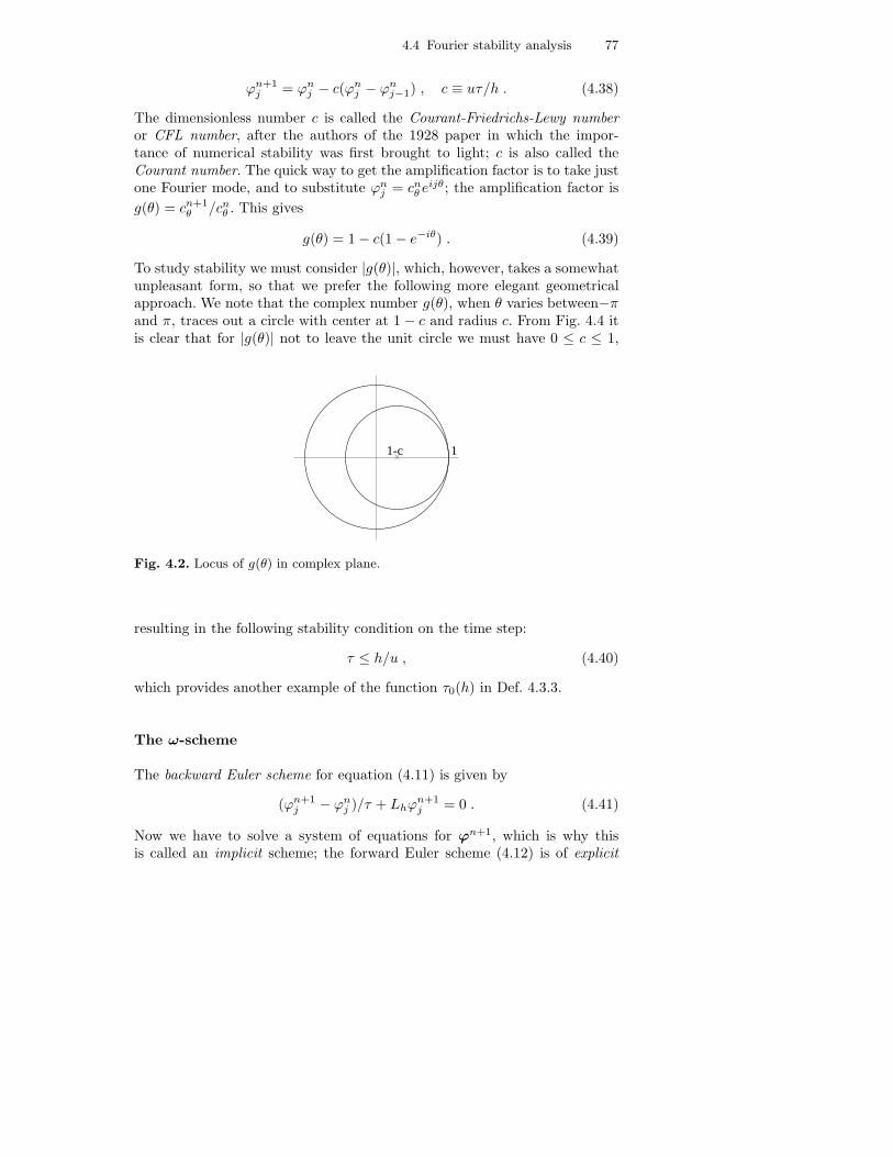
4.4 Fourier stability analysis 77
ϕn+1j = ϕn
j − c(ϕnj − ϕn
j−1) , c ≡ uτ/h . (4.38)
The dimensionless number c is called the Courant-Friedrichs-Lewy numberor CFL number, after the authors of the 1928 paper in which the impor-tance of numerical stability was first brought to light; c is also called theCourant number. The quick way to get the amplification factor is to take justone Fourier mode, and to substitute ϕn
j = cnθ eijθ; the amplification factor is
g(θ) = cn+1θ /cnθ . This gives
g(θ) = 1 − c(1 − e−iθ) . (4.39)
To study stability we must consider |g(θ)|, which, however, takes a somewhatunpleasant form, so that we prefer the following more elegant geometricalapproach. We note that the complex number g(θ), when θ varies between−πand π, traces out a circle with center at 1 − c and radius c. From Fig. 4.4 itis clear that for |g(θ)| not to leave the unit circle we must have 0 ≤ c ≤ 1,
11-c
Fig. 4.2. Locus of g(θ) in complex plane.
resulting in the following stability condition on the time step:
τ ≤ h/u , (4.40)
which provides another example of the function τ0(h) in Def. 4.3.3.
The ω-scheme
The backward Euler scheme for equation (4.11) is given by
(ϕn+1j − ϕn
j )/τ + Lhϕn+1j = 0 . (4.41)
Now we have to solve a system of equations for ϕn+1, which is why thisis called an implicit scheme; the forward Euler scheme (4.12) is of explicit

78 4. The nonstationary convection-diffusion equation
type. Therefore a time step with an implicit scheme requires much morecomputing work than an explicit scheme, but this may be compensated bybetter stability properties, allowing a larger time step. The global truncationerror of the Euler time stepping schemes (4.12) and (4.41) satisfies
e = O(τ + hm) ,
where m depends on the accuracy of the spatial discretization Lh. We canimprove this by taking a linear combination of the forward and backwardEuler schemes, as follows:
(ϕn+1jk − ϕn
jk)/τ + (1 − ω)Lhϕnjk + ωLhϕ
n+1jk = ωqn+1
jk + (1 − ω)qnjk , (4.42)
where we now assume the right-hand side q in (4.1) to be nonzero, and wherewe have gone to the two-dimensional case. This is called the ω-scheme. Forω = 1/2 this is called the Crank-Nicolson scheme, which is second order intime:
e = O(τ2 + hm) .
With the central scheme for convection, the space discretization of equation(4.1) is, with u, v, ε constant and uniform mesh sizes h1 and h2 in the x−and y−directions, respectively,:
Lhϕjk =u
2h1(ϕj+1,k − ϕj−1,k) +
v
2h2(ϕj,k+1 − ϕj,k−1)
+ε
h21
(−ϕj−1,k + 2ϕjk − ϕj+1,k) +ε
h22
(−ϕj,k−1 + 2ϕjk − ϕj,k+1) .
(4.43)
The equation for the perturbation δnjk is identical to the homogeneous version
(i.e. q = 0) of equation (4.43). For 1/2 < ω < 1 the stability analysis of theω-scheme is easy. As said before, the quick way to determine the amplificationfactor is to substitute δn
j = cnθ eijθ, where now j stands for j, k, and where
jθ = jθ1 + kθ2, cf. equation (4.25). Substitution gives
cn+1θ − cnθ + (1 − ω)τLh(θ)cnθ + ωτLh(θ)cn+1
θ = 0 ,
whereLh(θ) ≡ e−ijθLhe
ijθ .
It follows that
g(θ) =cn+1θ
cnθ=
1 − (1 − ω)τLh(θ)
1 + ωτLh(θ).
Let the real and imaginary part of the complex variable τLh be w1 and w2,respectively: τLh = w1 + iw2. Noting that for two complex numbers z1,2 we
have |z1/z2| = |z1|/|z2| and noting that |Lh|2 = w21 + w2
2, we get

4.4 Fourier stability analysis 79
|g(θ)|2 ≡ [1 − (1 − ω)w1]2 + (1 − ω)2w2
2
(1 + ωw1)2 + ω2w22
.
Assume that w1 ≥ 0. Then for 1/2 ≤ ω ≤ 1 the denominator is not smallerthan the numerator, so that |g(θ)| ≤ 1, and we have stability. To checkwhether w1 ≥ 0, we have to determine τLh. We find that
τLh = i(c1 sin θ1 + c2 sin θ2) + 2d1(1 − cos θ1) + 2d2(1 − cos θ2) , (4.44)
wherec1 ≡ uτ
h1, c2 ≡ vτ
h2, d1 ≡ ετ
h21
, d2 ≡ ετ
h22
,
from which it is obvious that w1 = Re(τLh) ≥ 0, ∀θ. Similarly, with theupwind scheme for convection we obtain, assuming u, v ≥ 0,
τLh = c1(1−e−iθ1)+c2(1−e−iθ2)+2d1(1−cosθ1)+2d2(1−cos θ2) , (4.45)
We have w1 = (c1 + 2d1)(1 − cos θ1) + (c2 + 2d2)(1 − cos θ2) ≥ 0 , ∀θ, sincec1,2 ≥ 0.
Hence, we have established unconditional stability of the ω-scheme for theconvection-diffusion equation, for 1/2 ≤ ω ≤ 1. The only interesting valuesof ω are 0, 1/2+O(τ), 1. The value ω = 0 is of interest because this gives anexplicit scheme, for which a time step is cheap. A value ω = 1/2 +O(τ) is ofinterest because this gives O(τ2) accuracy. Finally, ω = 1 is of interest becausethis is necessary for the discrete maximum principle in the nonstationary case;we will not go into this. Therefore we will not give stability conditions forthe ω-scheme for 0 ≤ ω < 1/2, but only for ω = 0. In this case the analysisbecomes a bit complicated, and we will give only the result; for a derivationsee Wesseling (2001) (Theorem 5.8.1). There it is shown that for the centralscheme a necessary and sufficient stability condition is:
2ετ( 1
h21
+1
h22
)
≤ 1 andτ
2ε(|u|2 + |v|2) ≤ 1 , (4.46)
and for the upwind scheme a sufficient stability condition is:
2ετ( 1
h21
+1
h22
+|u|
2εh1+
|v|2εh2
)
≤ 1 andτ
2ε
( |u|21 + |u|h1
+|v|2
1 + |v|h2
)
≤ 1 .
(4.47)It is left to the reader to verify that equations (4.36) and (4.40) are includedas special cases in (4.46) and (4.47), respectively.
Exercise 4.4.1. Suppose we have a numerical scheme for the convectionequation
80 4. The nonstationary convection-diffusion equation
∂ϕ
∂t+ c
∂ϕ
∂x= 0 , c constant ,
that has a stability condition cτ/h < C. What is the stability condition forthis scheme for the nonlinear case ∂ϕ/∂t+ ∂ϕm/∂x = 0?
Exercise 4.4.2. Derive equations (4.38) and (4.39).
Exercise 4.4.3. Show that scheme (4.38) is unconditionally unstable whenu < 0. (This is one way to see why the downwind scheme is bad).
Exercise 4.4.4. Discretize (4.37) with the central scheme in space and theforward Euler scheme in time. Show that the scheme is unconditionally un-stable.
Exercise 4.4.5. This exercise is meant to demonstrate the attractiveness ofthe geometric approach illustrated in Fig. 4.4. Determine |g(θ)|, with g(θ)given by equation (4.39). Use analysis instead of geometry to find conditionson c such that |g(θ)| ≤ 1, ∀θ.
Exercise 4.4.6. Derive equations (4.43)—(4.45).
Exercise 4.4.7. Write down the upwind version of scheme (4.43).
4.5 Numerical experiments
Problem statement
Some numerical experiments will be presented for the following one-dimensionaltest problem:
∂ϕ
∂t+ u
∂ϕ
∂x− ε
∂2ϕ
∂x2= q, 0 < x < 1, 0 < t ≤ T ,
q(t, x) = β2ε cosβ(x − ut) ,
(4.48)
with ε and u > 0 constant, and β a parameter. An exact solution is given by
ϕ(t, x) = cosβ(x− ut) + e−α2εt cosα(x − ut) , (4.49)
with α arbitrary. Spatial discretization is done with the second order centralor with the first order upwind scheme on the vertex-centered grid of Fig. 2.1with uniform mesh size h. For temporal discretization the ω-scheme is used.The resulting scheme can be written as
hj
τ(ϕn+1
j − ϕnj ) + ωLhϕ
n+1j + (1 − ω)Lhϕ
nj = hj [ωq
n+1j (1 − ω)qn
j ] , (4.50)
4.5 Numerical experiments 81
where hj is the volume of the cell over which is integrated. We choose aNeumann condition at x = 1, so that hj = h, j 6= J, hJ = h/2. In theinterior we get for the central scheme:
Lhϕj =Fj+1/2 − Fj−1/2 ,
Fj+1/2 =1
2u(ϕj+1 + ϕj) −
ε
h(ϕj+1 − ϕj) , j = 2, · · · , J − 1 .
(4.51)
At the Neumann boundary we integrate over a half cell, and obtain
FJ+1/2 = uϕJ − εb(t) ,
assuming a Neumann condition ∂ϕ(t, 1)/∂x = b(t).
Choice of time step, mesh size and time scale
The length scale L and time scale T of the exact solution are given by
L = π/max(α, β), T = minL/u, (εα2)−1 ,
where we take for the length scale of a harmonic function half its wavelength.We may expect accuracy to be sufficient if τ ≪ T , h ≪ L. For efficiency,we would like to avoid more stringent restrictions on τ and h, such as mightarise from stability. In the numerical experiments to be described we takeα = 4π, β = 2π, so that L ∼= 1/4. We take mostly h = 1/30, giving h/L ∼=0.13.
Remarks on the MATLAB program
The numerical experiments described below have been carried out with thecode cdns. The matrix Lh is described in Sect. 2.3 for the cell-centered case(called A there), and is easily adapted to the vertex-centered case. It is gen-erated (as in Sect. 2.3) by
L_h = spdiags([-beta0 beta0-beta1 beta1], -1:1, J, J);
The system to be solved for ϕn+1 with the ω-scheme (4.50) can be writtenas
Aφn+1 = Bφn + q . (4.52)
The matrices A and B can be generated by
x = linspace(0,1,J); % Grid node positions
hh = h*ones(size(x’));
hh(J,1) = h/2; % Last cell has half size
D = spdiags([hh/tau],0,J,J);
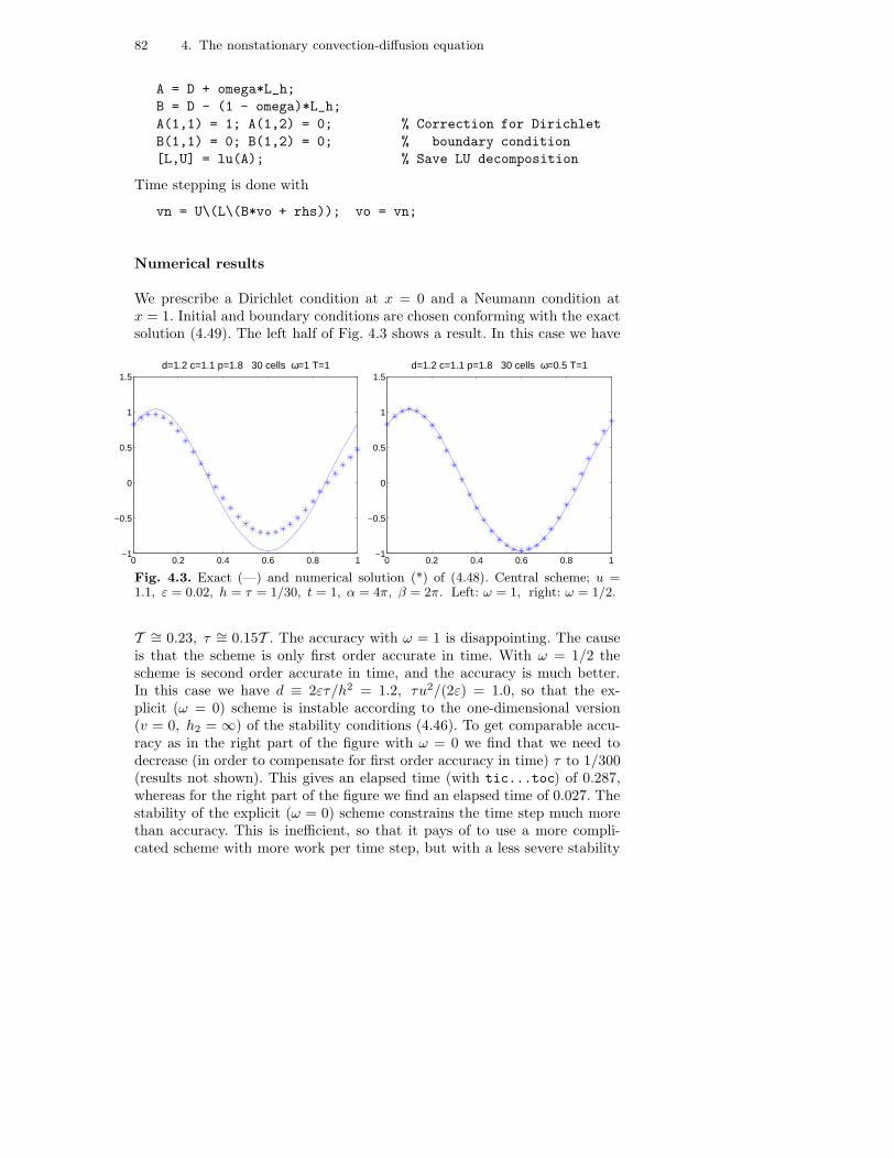
82 4. The nonstationary convection-diffusion equation
A = D + omega*L_h;
B = D - (1 - omega)*L_h;
A(1,1) = 1; A(1,2) = 0; % Correction for Dirichlet
B(1,1) = 0; B(1,2) = 0; % boundary condition
[L,U] = lu(A); % Save LU decomposition
Time stepping is done with
vn = U\(L\(B*vo + rhs)); vo = vn;
Numerical results
We prescribe a Dirichlet condition at x = 0 and a Neumann condition atx = 1. Initial and boundary conditions are chosen conforming with the exactsolution (4.49). The left half of Fig. 4.3 shows a result. In this case we have
0 0.2 0.4 0.6 0.8 1−1
−0.5
0
0.5
1
1.5d=1.2 c=1.1 p=1.8 30 cells ω=1 T=1
0 0.2 0.4 0.6 0.8 1−1
−0.5
0
0.5
1
1.5d=1.2 c=1.1 p=1.8 30 cells ω=0.5 T=1
Fig. 4.3. Exact (—) and numerical solution (*) of (4.48). Central scheme; u =1.1, ε = 0.02, h = τ = 1/30, t = 1, α = 4π, β = 2π. Left: ω = 1, right: ω = 1/2.
T ∼= 0.23, τ ∼= 0.15T . The accuracy with ω = 1 is disappointing. The causeis that the scheme is only first order accurate in time. With ω = 1/2 thescheme is second order accurate in time, and the accuracy is much better.In this case we have d ≡ 2ετ/h2 = 1.2, τu2/(2ε) = 1.0, so that the ex-plicit (ω = 0) scheme is instable according to the one-dimensional version(v = 0, h2 = ∞) of the stability conditions (4.46). To get comparable accu-racy as in the right part of the figure with ω = 0 we find that we need todecrease (in order to compensate for first order accuracy in time) τ to 1/300(results not shown). This gives an elapsed time (with tic...toc) of 0.287,whereas for the right part of the figure we find an elapsed time of 0.027. Thestability of the explicit (ω = 0) scheme constrains the time step much morethan accuracy. This is inefficient, so that it pays of to use a more compli-cated scheme with more work per time step, but with a less severe stability
83
restriction on the time step.
Exercise 4.5.1. Verify the stability conditions (4.46) by numerical experi-ments with the MATLAB program used in this section.
Exercise 4.5.2. Make a cell-centered version of the code cdns .
Some self-test questions
Write down the instationary convection-diffusion equation.
Formulate the maximum principle for the instationary convection-diffusion equation.
Write down the one-dimensional heat equation, discretize it with the forward Euler scheme andwrite down the matrix of the scheme.
Define the global and local truncation error for the instationary convection-diffusion equation.
Formulate Lax’s equivalence theorem.
Define zero-stability and absolute stability.
Write down the Fourier series for a grid function ∆j in d dimensions.
Write down the ω-scheme.
Which are the interesting values of ω for the ω-scheme? Why?
Show that the ω-scheme is unconditionally stable for ω ≥ 1/2.

5. The incompressible Navier-Stokes equations
5.1 Introduction
In this chapter, the incompressible Navier-Stokes equations in Cartesian co-ordinates discretized on Cartesian nonuniform grids will be considered, dis-cussing most of the basic numerical principles in a simple setting. In practicalapplications, of course, nonuniform grids and general coordinate systems areprevalent; these will not be discussed here; see Wesseling (2001).
We can be relatively brief in discussing discretization of the Navier-Stokesequations, because we prepared the ground in our extensive discussion of theconvection-diffusion equation in Chapters 2—4. Therefore it wil not be nec-essary to discuss again the various possibilities for discretizing convection, orstability conditions.
Only the primitive variable formulation will be discussed. This means thatthe velocity components and the pressure will be used as unknowns.
Purpose of this chapter
The purpose of this chapter is to present a numerical method for the incom-pressible Navier-Stokes equations. In particular, we will:
• Present suitable boundary conditions;• Describe spatial discretization on a staggered grid;• Describe the ω-scheme, the Adams-Bashforth scheme and the Adams-Bashforth-ω scheme for discretization in time;• Show how to linearize with the Picard or Newton method;• Describe the pressure-correction method;• Discuss stability conditions;• Present some numerical experiments with the MATLAB codes ns1 andns2;• Discuss outflow boundary conditions;• Discuss efficiency.
86 5. The incompressible Navier-Stokes equations
5.2 Equations of motion and boundary conditions
Equations of motion
We restrict ourselves to the two-dimensional case. The equations of motionhave been discussed in Chap. 1. For ease of reference, the equations to beconsidered are repeated here. We assume incompressible flow, i.e.Dρ/Dt = 0,so that (cf. (1.8))
ux + vy = 0 , (5.1)
where we denote partial differentiation by a subscript. The density is takenconstant. The dimensionless incompressible Navier-Stokes equations are givenby equation (1.23):
ut + uux + vuy = −px + Re−1(uxx + uyy) ,
vt + uvx + vvy = −py + Re−1(vxx + vyy) .(5.2)
By adding u(ux + vy) and v(ux + vy) (both zero according to (5.1)), respec-tively, this can be put in conservation form:
ut + (uu)x + (vu)y = −px + Re−1(uxx + uyy) ,
vt + (uv)x + (vv)y = −py + Re−1(vxx + vyy) .(5.3)
The following units are chosen: velocity: U ; length: L; density: ρ0; pressure:ρ0U
2. Then the Reynolds number is given by
Re = ρ0UL/µ ,
with µ the dynamic viscosity coefficient, which was already assumed to beconstant above.
The deviatoric stress tensor (i.e. the viscous part of the stress tensor) isdenoted by σαβ . From equation (1.15) it follows that
σxx = 2Re−1ux, σxy = σyx = Re−1(uy + vx), σyy = 2Re−1vy . (5.4)
The governing equations (5.1) and (5.2) need to be accompanied by initialand boundary conditions.
Initial conditions
For the momentum equations (5.2) the following initial conditions are re-quired:
u(0,x) = u0(x) , v(0,x) = v0(x) ,
with the prescribed initial velocity field u0 satisfying the continuity equation(5.1). Note that there is no initial condition for the pressure, since pt doesnot occur.
5.2 Equations of motion and boundary conditions 87
No-slip condition
Viscous fluids cling to solid surfaces. This is called the no-slip condition. Ata solid surface we have
u(t,x) = v(t,x) , (5.5)
with v(t,x) the local wall velocity. The Dirichlet condition (5.5) holds alsoat open parts of the boundary where the velocity is prescribed, which maybe the case at an inflow boundary. But at an inflow boundary one may alsoprescribe condition (5.6) given below.
Free surface conditions
At a free surface the tangential stress components are zero. We consider onlythe very special case where the free surface is fixed at y = a = constant. Forthe general case, see Sect. 6.2 of Wesseling (2001). At a fixed free surface, thenormal velocity and the tangential stress are zero:
v(t, x, a) = 0, uy(t, x, a) = 0 , (5.6)
where we have used
σxy(t, x, a) = Re−1(uy + vx)(t, x, a) = Re−1uy(t, x, a) .
We see that we have a Dirichlet condition for the normal velocity and a Neu-mann condition for the tangential velocity. A truly free surface moves, itsshape must be determined and follows from the condition that the normalstress equals the ambient pressure. This case will not be considered. Condi-tions (5.6) may also arise at a plane of symmetry. In special cases one maywish to prescribe non-zero tangential stress in (5.6), for example, when onewishes to take the influence of wind shear on a water surface into account.
Inflow conditions
The momentum equations resemble convection-diffusion equations for uand v, so that the insights gained in the convection-diffusion equation inChapt. 2—4 provide guidelines for numerical approximation. Based on whatwe learned about the convection-diffusion equation, we prescribe Dirichletconditions at an inflow boundary. If, for example, x = 0 is an inflow bound-ary, we prescribe
u(t, 0, y) = U(t, y) , v(t, 0, y) = V (t, y) . (5.7)
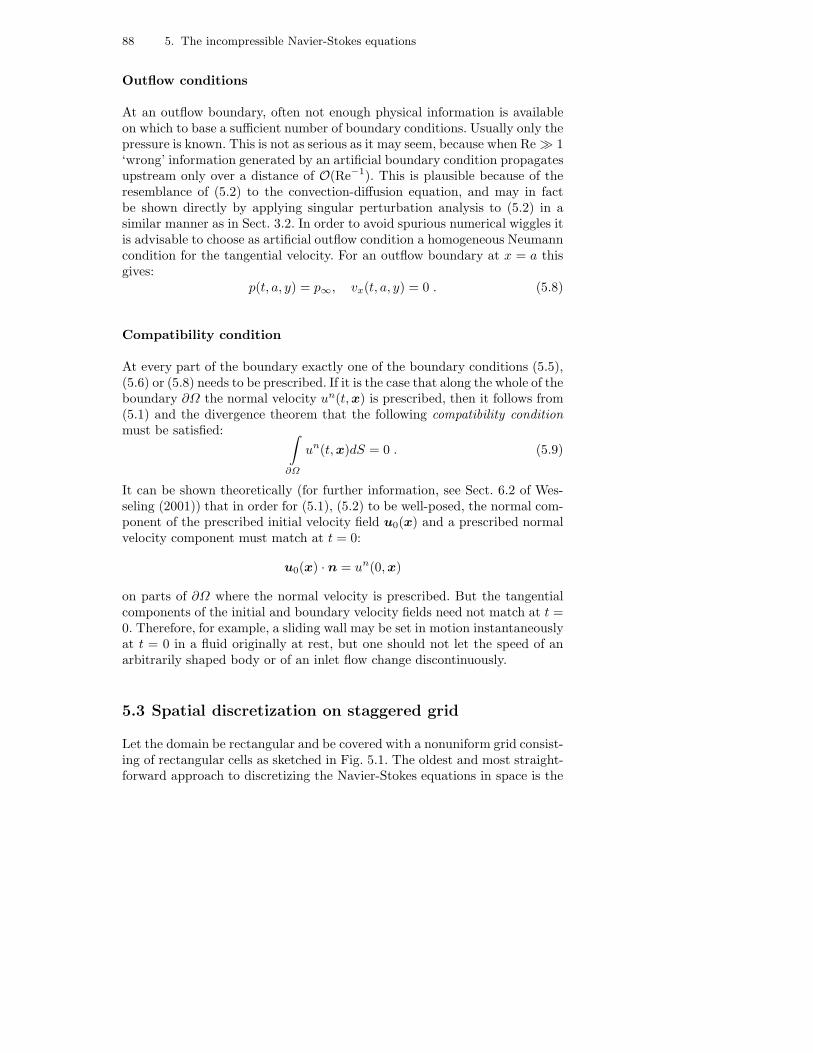
88 5. The incompressible Navier-Stokes equations
Outflow conditions
At an outflow boundary, often not enough physical information is availableon which to base a sufficient number of boundary conditions. Usually only thepressure is known. This is not as serious as it may seem, because when Re ≫ 1‘wrong’ information generated by an artificial boundary condition propagatesupstream only over a distance of O(Re−1). This is plausible because of theresemblance of (5.2) to the convection-diffusion equation, and may in factbe shown directly by applying singular perturbation analysis to (5.2) in asimilar manner as in Sect. 3.2. In order to avoid spurious numerical wiggles itis advisable to choose as artificial outflow condition a homogeneous Neumanncondition for the tangential velocity. For an outflow boundary at x = a thisgives:
p(t, a, y) = p∞, vx(t, a, y) = 0 . (5.8)
Compatibility condition
At every part of the boundary exactly one of the boundary conditions (5.5),(5.6) or (5.8) needs to be prescribed. If it is the case that along the whole of theboundary ∂Ω the normal velocity un(t,x) is prescribed, then it follows from(5.1) and the divergence theorem that the following compatibility conditionmust be satisfied:
∫
∂Ω
un(t,x)dS = 0 . (5.9)
It can be shown theoretically (for further information, see Sect. 6.2 of Wes-seling (2001)) that in order for (5.1), (5.2) to be well-posed, the normal com-ponent of the prescribed initial velocity field u0(x) and a prescribed normalvelocity component must match at t = 0:
u0(x) · n = un(0,x)
on parts of ∂Ω where the normal velocity is prescribed. But the tangentialcomponents of the initial and boundary velocity fields need not match at t =0. Therefore, for example, a sliding wall may be set in motion instantaneouslyat t = 0 in a fluid originally at rest, but one should not let the speed of anarbitrarily shaped body or of an inlet flow change discontinuously.
5.3 Spatial discretization on staggered grid
Let the domain be rectangular and be covered with a nonuniform grid consist-ing of rectangular cells as sketched in Fig. 5.1. The oldest and most straight-forward approach to discretizing the Navier-Stokes equations in space is the
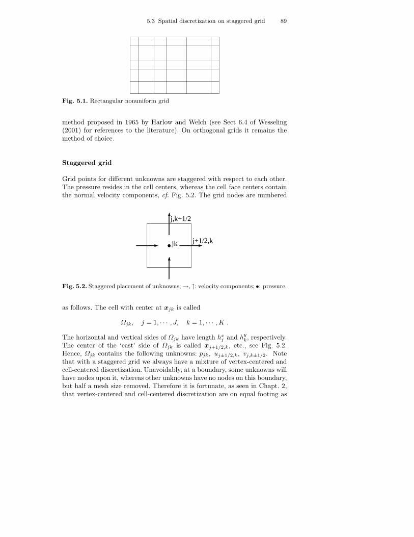
5.3 Spatial discretization on staggered grid 89
Fig. 5.1. Rectangular nonuniform grid
method proposed in 1965 by Harlow and Welch (see Sect 6.4 of Wesseling(2001) for references to the literature). On orthogonal grids it remains themethod of choice.
Staggered grid
Grid points for different unknowns are staggered with respect to each other.The pressure resides in the cell centers, whereas the cell face centers containthe normal velocity components, cf. Fig. 5.2. The grid nodes are numbered
jk j+1/2,k
j,k+1/2
Fig. 5.2. Staggered placement of unknowns; →, ↑: velocity components; •: pressure.
as follows. The cell with center at xjk is called
Ωjk, j = 1, · · · , J, k = 1, · · · ,K .
The horizontal and vertical sides of Ωjk have length hxj and hy
k, respectively.The center of the ‘east’ side of Ωjk is called xj+1/2,k, etc., see Fig. 5.2.Hence, Ωjk contains the following unknowns: pjk, uj±1/2,k, vj,k±1/2. Notethat with a staggered grid we always have a mixture of vertex-centered andcell-centered discretization. Unavoidably, at a boundary, some unknowns willhave nodes upon it, whereas other unknowns have no nodes on this boundary,but half a mesh size removed. Therefore it is fortunate, as seen in Chapt. 2,that vertex-centered and cell-centered discretization are on equal footing as
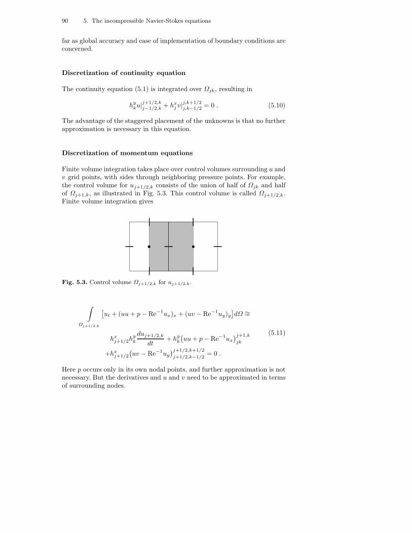
90 5. The incompressible Navier-Stokes equations
far as global accuracy and ease of implementation of boundary conditions areconcerned.
Discretization of continuity equation
The continuity equation (5.1) is integrated over Ωjk, resulting in
hyku|
j+1/2,kj−1/2,k + hx
j v|j,k+1/2j,k−1/2 = 0 . (5.10)
The advantage of the staggered placement of the unknowns is that no furtherapproximation is necessary in this equation.
Discretization of momentum equations
Finite volume integration takes place over control volumes surrounding u andv grid points, with sides through neighboring pressure points. For example,the control volume for uj+1/2,k consists of the union of half of Ωjk and halfof Ωj+1,k, as illustrated in Fig. 5.3. This control volume is called Ωj+1/2,k.Finite volume integration gives
Fig. 5.3. Control volume Ωj+1/2,k for uj+1/2,k.
∫
Ωj+1/2,k
[
ut + (uu+ p− Re−1ux)x + (uv − Re−1uy)y
]
dΩ ∼=
hxj+1/2h
yk
duj+1/2,k
dt+ hy
k
(
uu+ p− Re−1ux
)j+1,k
jk
+hxj+1/2
(
uv − Re−1uy
)j+1/2,k+1/2
j+1/2,k−1/2= 0 .
(5.11)
Here p occurs only in its own nodal points, and further approximation is notnecessary. But the derivatives and u and v need to be approximated in termsof surrounding nodes.
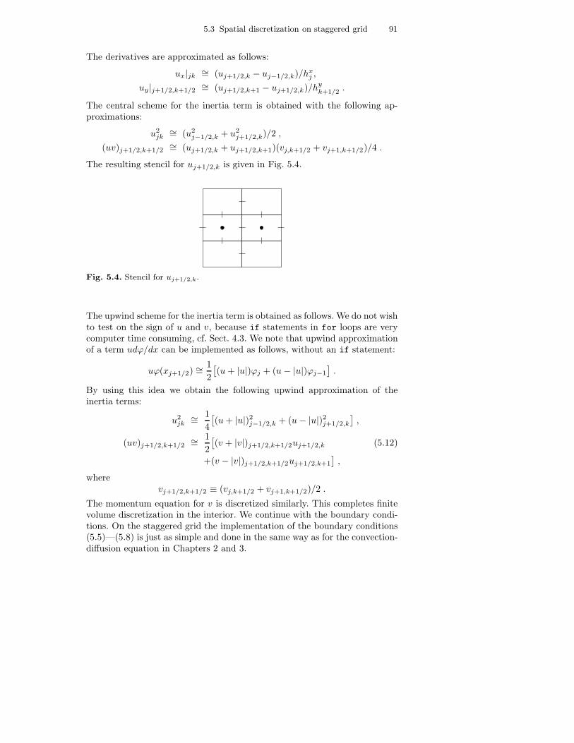
5.3 Spatial discretization on staggered grid 91
The derivatives are approximated as follows:
ux|jk∼= (uj+1/2,k − uj−1/2,k)/hx
j ,
uy|j+1/2,k+1/2∼= (uj+1/2,k+1 − uj+1/2,k)/hy
k+1/2 .
The central scheme for the inertia term is obtained with the following ap-proximations:
u2jk
∼= (u2j−1/2,k + u2
j+1/2,k)/2 ,
(uv)j+1/2,k+1/2∼= (uj+1/2,k + uj+1/2,k+1)(vj,k+1/2 + vj+1,k+1/2)/4 .
The resulting stencil for uj+1/2,k is given in Fig. 5.4.
Fig. 5.4. Stencil for uj+1/2,k.
The upwind scheme for the inertia term is obtained as follows. We do not wishto test on the sign of u and v, because if statements in for loops are verycomputer time consuming, cf. Sect. 4.3. We note that upwind approximationof a term udϕ/dx can be implemented as follows, without an if statement:
uϕ(xj+1/2) ∼=1
2
[
(u+ |u|)ϕj + (u − |u|)ϕj−1
]
.
By using this idea we obtain the following upwind approximation of theinertia terms:
u2jk
∼= 1
4
[
(u+ |u|)2j−1/2,k + (u− |u|)2j+1/2,k
]
,
(uv)j+1/2,k+1/2∼= 1
2
[
(v + |v|)j+1/2,k+1/2uj+1/2,k (5.12)
+(v − |v|)j+1/2,k+1/2uj+1/2,k+1
]
,
wherevj+1/2,k+1/2 ≡ (vj,k+1/2 + vj+1,k+1/2)/2 .
The momentum equation for v is discretized similarly. This completes finitevolume discretization in the interior. We continue with the boundary condi-tions. On the staggered grid the implementation of the boundary conditions(5.5)—(5.8) is just as simple and done in the same way as for the convection-diffusion equation in Chapters 2 and 3.
92 5. The incompressible Navier-Stokes equations
The no-slip condition
Let y = 0 be a wall moving horizontally with velocity U(t). Then the lowerside of Ωj,1 is at the boundary. We have vj,1/2 = 0, so that no discretizationfor vj,1/2 is required. In the finite volume scheme for uj+1/2,1 we need, ac-cording to the stencil presented in Fig. 5.4, uj+1/2,0, which is not available,because xj+1/2,0 is outside the domain. Values outside the domain are calledvirtual values.We write uj+1/2,0 + uj+1/2,1 = 2U(t), so that
uj+1/2,0 = 2U(t) − uj+1/2,1 , (5.13)
which is used to eliminate the virtual value uj+1/2,0.
Free surface conditions
Let y = a be a free surface boundary or a symmetry boundary, so that wehave conditions (5.6). Let Ωjk be at the boundary. We have vj,K+1/2 = 0, sothat no discrete equation is required for vj,K+1/2. In the stencil for uj+1/2,K
we have uj+1/2,K+1, according to Fig. 5.4, which is outside the domain andhas to be eliminated. We put 0 = uy
∼= (uj+1/2,K+1 − uj+1/2,K)/hyK , so that
uj+1/2,K+1 = uj+1/2,K . (5.14)
Inflow conditions
Let x = 0 be an inflow boundary, so that Ω1k is at the boundary. Accordingto (5.7) we have Dirichlet conditions for u and v, so that the situation isalmost the same as for the no-slip condition. We put
u1/2,k = U(t, yk) , v0,k+1/2 = 2V (t, yk+1/2) − v1,k+1/2 . (5.15)
Outflow conditions
Let ΩJk be at an outflow boundary x = a. We need discrete equations foruJ+1/2,k and vJ,k+1/2. The control volume for uJ+1/2,k consists of half of ΩJk,as illustrated in Fig. 5.5. Finite volume integration gives, similar to (5.11),
∫
ΩJ+1/2,k
[
ut +(uu+ p− Re−1ux)x + (uv − Re−1uy)y
]
dΩ ∼=
12h
xJh
ykduJ+1/2,k/dt+ hy
k
(
uu+ p− Re−1ux
)J+1/2,k
Jk
+ 12h
xJ
(
uv − Re−1uy
)J+1/2,k+1/2
J+1/2,k−1/2= 0 .

5.3 Spatial discretization on staggered grid 93
Fig. 5.5. Control volumes for uJ+1/2,k and vJ,k+1/2 at outflow boundary.
Compared to the interior case, we have to change only terms at or nearthe outflow boundary. We put the normal stress at xJ+1/2,k equal to theprescribed pressure (cf. (5.8)):
(p− Re−1ux)J+1/2,k = p∞ .
Furthermore,(uv)J+1/2,k+1/2 = vJ,k+1/2uJ+1/2,k+1/2 ,
where uJ+1/2,k+1/2 is approximated with the upwind scheme or the centralscheme. Finally,
Re−1(uy)J+1/2,k+1/2∼= (uJ+1/2,k+1 − uJ+1/2,k)/hy
J+1/2,k+1/2 .
The scheme for vJ,k+1/2 brings nothing new. A virtual value vJ+1,k+1/2 oc-curs as may be seen form the stencil of the v-momentum equation, which isobtained from Fig. 5.4 by rotation over 90o. This virtual value is eliminatedby using vx = 0 (cf. (5.8)), which results in
vJ+1,k+1/2 = vJ,k+1/2
(cf. (5.14)).
Summary of equations
We put all unknown velocity components in some order in an algebraic vectoru and all pressure unknowns in an algebraic vector p, and we divide by thecoefficients of the time derivatives. Then the scheme can be written as adifferential-algebraic system of the following structure:
du
dt+N(u) +Gp = f(t) , Du = g(t) . (5.16)
Here N is a nonlinear algebraic operator arising from the discretization ofthe inertia and viscous terms, G is a linear algebraic operator representingthe discretization of the pressure gradient, D is a linear algebraic operator
94 5. The incompressible Navier-Stokes equations
representing the discretization of divergence operator in the continuity equa-tion, and f and g are known source terms, arising from the boundary con-ditions. This is called a differential-algebraic system because it is a mixtureof a system of ordinary differential equations (the first member of (5.16)),and algebraic equations (the second member of (5.16)). This completes ourdescription of spatial discretization on the staggered grid.
5.4 Temporal discretization on staggered grid
We now discretize also in time. Equation (5.16) is our point of departure.With the forward Euler scheme we obtain:
1
τ(un − un−1) +N(un−1) +Gpn−1/2 = f(tn−1) , Dun = g(tn) . (5.17)
Note that we have to take the pressure term at the new time tn, or for betteraccuracy in time, at tn−1/2, in order to have degrees of freedom to satisfy thealgebraic solenoidality constraint (second equation of (5.17)). In other words,the pressure always has to be taken implicitly; this is a consequence of thedifferential-algebraic nature of (5.16). In incompressible flows, the pressureacts as a Lagrange multiplier, that makes it possible to satisfy the continuityequation.
With the ω-scheme we obtain:
1
τ(un − un−1)+ωN(un) + (1 − ω)N(un−1) +Gpn−1/2
=ωf(tn) + (1 − ω)f(tn−1) , Dun = g(tn) .(5.18)
Linearization
Equation (5.18) is a nonlinear system, because the nonlinear inertia termmakes the operator N nonlinear. To make the system more easily solvablewe linearize the operator N . Newton linearization works as follows, writingδu = un − un−1:
N(un) = N(un−1 + δu) ∼= N(un−1) + C(un−1)δu ,
where C(u) is the Jacobian of N evaluated at u. We clarify this by taking asan example one term of the inertia term (cf. (5.11)):
(un+1jk )2 = (un
jk + δujk)2 ∼= (unjk)2 + 2un
jkδujk .
We eliminate δu and obtain:
(un+1jk )2 ∼= 2un
jkun+1jk − (un
jk)2 ,

5.4 Temporal discretization on staggered grid 95
which is linear in the unknown un+1jk . Picard linearization works as follows:
(un+1jk )2 ∼= un
jkun+1jk .
This is simpler, but temporal accuracy decreases to O(τ). A second orderaccurate approximation is obtained if one replaces un by an extrapolation totn+1:
(un+1jk )2 ∼= (2un
jk − un−1jk )un+1
jk . (5.19)
We will call this extrapolated Picard linearization.
After linearization, the matrix C that one obtains changes every time step,because C depends on un−1. Matrix generation is computer time consuming.Therefore a time step will be cheaper if the inertia term is discretized explic-itly. This gives us a so-called IMEX (implicit-explicit) scheme. The resultingscheme is cheaper, because the implicit operator is now linear and indepen-dent of time, so that the corresponding matrix has to be generated only once,and other ingredients necessary for solving, such as an LU factorization, needalso to be prepared only once. To maintain second order accuracy in time, itis attractive to use for the explicit part not the forward Euler scheme, buta second order explicit scheme, such as the Adams-Bashforth scheme. For asystem of ordinary differential equations dw/dt = f(w, t) this scheme is givenby
1
τ(wn − wn−1) =
3
2f(wn−1, tn−1) − 1
2f(wn−2, tn−2) . (5.20)
This is called a two-step method, because two time steps are involved. At theinitial time t = 0 one may define w−1 = w0. Application to the Navier-Stokesequations takes place as follows. Let N(u) in (5.18) be split in a nonlinearinertia part C and a linear viscous part B, as follows:
N(u) = C(u) +Bu .
Then the Adams-Bashforth-Crank-Nicolson scheme is obtained by using(5.18) for Bu and (5.20) for C(u), so that we obtain:
1
τ(un − un−1)+ 3
2C(un−1) − 12C(un−2) + 1
2B(un + un−1) +Gpn−1/2
= f(tn+1/2) , Dun = g(tn) .
General formulation on staggered grid
As seen from these examples, time stepping methods applied to equation(5.11) can generally be written as
A(un) + τGpn−1/2 = rn ,
Dun = g(tn) ,(5.21)
96 5. The incompressible Navier-Stokes equations
where rn is known from previous time steps and the boundary conditions. Forexplicit methods, A is the identity I. The system (5.21) is a coupled systemfor un and pn−1/2. Computing time is reduced if pn−1/2 and un can be solvedfor separately. To this end the following method has been devised, which isthe method of choice for nonstationary problems.
Pressure-correction method
Equation (5.21) is not solved as it stands, but first a prediction u∗ of un ismade that does not satisfy the continuity equation. Then a correction is com-puted involving the pressure, such that the continuity equation is satisfied.The method is given by:
A(u∗) + τGpn−3/2 = rn , (5.22)
un − u∗ + τG(pn−1/2 − pn−3/2) = 0 , (5.23)
Dun = g(tn) . (5.24)
Equation (5.22) more or less amounts to solving discretized convection-diffusion equations for the predicted velocity components. We use the bestavailable guess for the pressure, namely pn−3/2. Equation (5.23) is motivatedby the fact, that if in the explicit case, where A is the identity, we eliminateu∗ from (5.22) and (5.23), then the original system (5.21) is recovered. Thepressure can be computed by applying the operator D to (5.23) and using(5.24), resulting in
DGδp =1
τDu∗ − g(tn), pn−1/2 = pn−3/2 + δp . (5.25)
After pn−1/2 has been computed, un follows from (5.23).
Equation (5.23) can be regarded as a correction of u∗ for the change inpressure. Therefore (5.22)–(5.25) is called the pressure-correction method. Itis an example of a fractional step method, in which a time step is split upin sub-steps, and different physical effects are accounted for separately inthe sub-steps. Here pressure forces are accounted for in the second sub-step,and inertia and friction in the first sub-step. Confusingly, the term pressure-correction method is often also applied to various iterative methods to solvethe stationary Navier-Stokes equations, in which velocity and pressure up-dates are carried out not simultaneously but successively. Such methods willbe encountered in Chap. 6, where they will be called distributive iterationmethods. These should not be confused with the pressure-correction methodused in time accurate schemes as formulated above. This method may alsobe called a projection method, because in (5.23) the new velocity un is theprojection of the intermediate velocity field u∗ on the space of velocity fieldswith discretized divergence equal to zero.

5.4 Temporal discretization on staggered grid 97
Remembering that divgrad equals the Laplacian, we see that (5.25) looksvery much like a discrete Poisson equation; it is frequently called the pres-sure Poisson equation. Note that no boundary condition needs to be invokedfor δp (fortunately, for no such condition is given with the original equations,at least not on the complete boundary), because the boundary conditionshave already been taken into account in the construction of D, G and g;the operator DG works exclusively on pressure values at grid points in theinterior of the domain.
Even if the method is explicit (A is a diagonal matrix), we still have tosolve an implicit system for δp. This is an unavoidable consequence of thedifferential-algebraic nature of (5.16).
As we remarked before, by elimination of u∗ it is easily seen that in theexplicit case the pressure-correction method (5.22)–(5.25) is equivalent to(5.21), and that this remains true if pn−3/2 is neglected in (5.22) and (5.23).But in the implicit case this does not hold, and inclusion of a sufficientlyaccurate first guess, such as pn−3/2, for the pressure in (5.22) seems to benecessary to obtain full, i.e. O(τ2), temporal accuracy. This may make itnecessary to compute the initial pressure field at the starting step (n = 1),to be used instead of p−1/2. This may be done as follows. Application of Dto (5.16) at t = 0 gives
dg(0)/dt+DN(u(0)) +DGp(0) = Df(0) . (5.26)
After solving p(0) from (5.26), we put p−1/2 = p(0).
Discrete compatibility condition
In case the pressure is not involved in any of the boundary conditions, itfollows from the incompressible Navier-Stokes equations that the pressure isdetermined up to a constant. The system (5.25) for δp is singular in this case,and (5.25) has a solution only if the right-hand side satisfies a compatibilitycondition. The boundary conditions discussed in Sect. 5.2 are such that ifthe pressure is not involved in any of the boundary conditions, then thenormal velocity component is prescribed all along the boundary, and thecompatibility condition (5.9) is satisfied. Summing the discrete continuityequation (5.10) over all cells reduces, due to cancellation in the interior, tothe following sum over boundary points:
K∑
k=1
hyku
∣
∣
∣
(J+1/2,k)
(1/2,k)+
J∑
j=1
hxj v
∣
∣
∣
(j,K+1/2)
(j,1/2)= 0 , (5.27)
where u and v are the prescibed velocity components at the boundary. If(5.27) is not satisfied exactly one should adjust u and v at the boundaries,
98 5. The incompressible Navier-Stokes equations
which should not be difficult, because of the compatibility condition (5.9). If(5.27) holds, then it turns out that the elements of the right-hand side vectorof (5.25) sum to zero, which is precisely the compatibility condition requiredfor existence of solutions of (5.25). If one desires to make the solution uniqueone can fix δp in some point, but iterative methods usually converge faster ifone lets δp float.
Temporal accuracy
For literature on the accuracy of the pressure-correction method, see Wes-seling (2001), Sect. 6.6 and references quoted there. Indications are that thetemporal accuracy of un is of the same order as rhe order of accuracy of theunderlying time stepping method (for example, O(τ2) for Adams-Bashforth-Crank-Nicolson), but that the accuracy of pn−1/2 is only O(τ), irrespective ofthe time stepping method used. If one desires, a pressure field with improvedaccuracy can be obtained after un has been computed (with the pressure-correction method) by proceeding in the same way as in the derivation of(5.26), leading to the following equation for pn−1/2:
dg(tn)/dt+DN(un) +DGpn−1/2 = Df(tn) ,
which very likely results in a pressure field pn−1/2 with the same order oftemporal accuracy as the velocity field.
Stability
For stability of (5.22)—(5.25), it seems necessary that (5.22) is stable. It isconjectured that this is sufficient for the stability of (5.22)—(5.25); numericalevidence supports this conjecture. We restrict ourselves to Fourier stabilityanalysis of (5.22). To this end (5.22) is linearized, the coefficients are takenconstant (‘frozen’), the boundary conditions are assumed to be periodic, andthe known source terms τGpn−3/2 and rn are neglected. Hence, carryingout Fourier stability analysis for (5.22) implies that the discretization of thefollowing simplified and linearized version of (5.2) is considered:
ut + Uux + V uy − Re−1(uxx + uyy) = 0 ,
vt + Uvx + V vy − Re−1(vxx + vyy) = 0 ,(5.28)
Equation (5.28) consists of decoupled and identical convection-diffusion equa-tions, for which Fourier stability analysis is presented in Chap. 4. The stabilityanalysis of the Adams-Bashforth-Crank-Nicolson scheme is a bit involved andis not presented in Chap. 4. In Sect. 6.6 of Wesseling (2001) stability condi-tions for the Adams-Bashforth-Crank-Nicolson scheme are derived. With thecentral scheme for the inertia terms we have:
5.5 Numerical experiments 99
τ ≤ max[τ1,minτ2, τ3] ,
τ1 ≡ 4
3Re
[
U2 + V 2]−1
,
τ2 ≡ Re
4
[
(hx)−2 + (hy)−2]−1
,
τ3 ≡( 3
Re
)1/3[(U2/hx)2/3 + (V 2/hy)2/3
]−1.
(5.29)
For the upwind scheme:
τ ≤ max[τ1,minτ2, τ3] ,
τ1 ≡ 2
3Re
[ U2
2 + UhxRe+
V 2
2 + V hyRe
]−1
,
τ2 ≡ Re
4
[1 + UhxRe/2
(hx)2+
1 + V hyRe/2
(hy)2
]−1
,
τ3 ≡( 3
Re
)1/3[( U4
(hx)2 + U(hx)3Re/2
)1/3
+( V 4
(hy)2 + V (hy)3Re/2
)1/3]−1
.
(5.30)
The computing cost of checking in every grid point whether the stability con-dition is satisfied is often not negligible, so in practice this is often done onlyevery 5 or 10 time steps or so, or only once, if one has a reasonable a prioriestimate of U (= 2 max(u)) and V (= 2 max(v)). Here the factor 2 arisesfrom the nonlinearity of the inertia terms, in the same way as for the Burgersequation in Sect. 4.4.
Exercise 5.4.1. What is the Newton linearization of uv?
5.5 Numerical experiments
The schemes just described have been implemented in the MATLAB codesns1 (ω-scheme) and ns2 (Adams-Bashforth-ω-scheme), on a nonuniformCartesian grid of the type shown in Fig. 5.1. For ns1, Picard linearization orextrapolated Picard linearization is used for the inertia terms. Three typesof boundary conditions have been implemented: inflow, outflow and no-slip.The boundaries can be divided in segments, on which one can choose differ-ent boundary conditions and numbers of grid cells. For instance, we can dothe so-called backward-facing step problem, illustrated in Fig. 5.6. Becausethe domain is assumed to be rectangular, we cannot handle the narrow in-flow part at the left, and use the rectangular domain shown at the right. Wechoose |AB| = |BC| = 1, |CD| = L, with L to be chosen. It turns out that arecirculation zone is present attached to BC, with length dependent on theReynolds number Re. The length of the domain L must be larger than the

100 5. The incompressible Navier-Stokes equations
A
B
C D
E
Fig. 5.6. The backward-facing step problem.
length of the recirculation zone, in order to have u > 0 at DE, so that theoutflow boundary condition (5.8) is appropriate. Let the Reynolds number bebased on the length of AB and the average inflow velocity. On the segmentAB we prescribe inflow: v = 0, u = f(y), f parabolic, such that the aver-age inflow velocity is 1. On DE we prescribe outflow, and on the remainingboundary segments no-slip. The grid is uniform with nx× ny cells.
Wrong outflow conditions
First, we prescribe Dirichlet conditions, namely a parabolic outflow profile:
u = g(y), v = 0 (5.31)
on the outflow boundary DE. This is against the advice given concerningoutflow boundary conditions in Sect. 5.2. Let us see what goes wrong. Fig.5.7 shows a result, using Picard linearization. Note that the horizontal andvertical scales are different in the left part of the figure. The relative change
0 2 4 6 8 10 120
0.5
1
1.5
2Streamlines
0 200 400 600 800 100010
−3
10−2
10−1
100
101
102
Relative change per time step
Fig. 5.7. Streamlines and convergence history for backward-facing step problem,code ns1, Dirichlet outflow conditions. Re = 100, τ = 0.2, t = 190, nx = 30, ny =20, ω = 1, central scheme.

5.5 Numerical experiments 101
per time step is defined as
1
dtmax
[‖ un+1 − un ‖qn+1
,‖ vn+1 − vn ‖
qn+1,
‖ pn+1 − pn ‖‖ pn ‖ +(qn+1)2/2
]
,
where q = max(‖ u ‖, ‖ v ‖), and the maximum norm is used. In the left partof the figure, we observe unphysical wiggles near the outflow boundary, andthe convergence history shows that the solution hesitates to become reallystationary. The cause of the wiggles and the remedy have been discussed inSect. 5.2. For Re = 200 a stationary solution was not obtained. Furthermore,it was found that with extrapolated Picard linearization, convergence to asteady solution did not take place.
Further results on the backward facing step problem
From now on, we use extrapolated Picard linearization. With the correct out-flow boundary conditions (5.8) the result shown in Fig. 5.8 is obtained. This
0 2 4 6 8 10 120
0.5
1
1.5
2Streamlines
0 20 40 60 80 10010
−5
10−4
10−3
10−2
10−1
100
Relative change per time step
Fig. 5.8. Streamlines and convergence history for backward-facing step problem,code ns1, outflow conditions(5.8) . Re = 100, τ = 0.6, t = 60, nx = 30, ny = 20, ω =1, central scheme.
result looks more satisfactory. The length of the recirculation region agreeswith results reported in the literature, and the solution seems to evolve tosteady state. Due to the use of Picard linearization, ns1 it is not uncondi-tionally stable; we know no guidelines for choosing the time step τ . For linearproblems, the ω-scheme with ω = 1 is unconditionally stable, as seen in Sect.4.4.
Fig. 5.9 shows what happens when the Reynolds number is increased. Thelength of the recirculation region increases; it is thought to be proportional

102 5. The incompressible Navier-Stokes equations
0 2 4 6 8 10 120
0.5
1
1.5
2Streamlines
0 20 40 60 80 10010
−3
10−2
10−1
100
Relative change per time step
Fig. 5.9. Streamlines and convergence history for backward-facing step problem,code ns1. Re = 200, τ = 0.6, t = 60, nx = 30, ny = 20, ω = 1, central scheme.
to the Reynolds number. This flow we have also computed with the Adams-Bashforth-ω scheme (code ns2). The flow pattern obtained is the same as inFig. 5.9. To determine the time step τ we have used the stability criterionfor the Adams-Bashforth-Crank-Nicolson scheme (hence, ω = 1/2) presentedin Sect. 4.4, taking for safety τ 20% smaller than allowed, giving τ = 0.021.The convergence history is shown in Fig. 5.10. Although the time required
0 500 1000 1500 2000 250010
−3
10−2
10−1
100
Relative change per time step
Fig. 5.10. Convergence history for backward-facing step problem, code ns2.
to execute a time step with ns1 is seven times larger than for ns2 (why isit larger, you think?), ns1 is faster because its time step is much larger. Therecirculation length in Fig. 5.9 agrees with reports in the literature. With theupwind scheme the recirculation length is found to 7, which is too small. Thisis because the upwind scheme adds artificial viscosity, and the recirculationlength is known to increase with decreasing viscosity.

5.5 Numerical experiments 103
The case Re = 400, shown in Fig. 5.11 is found to be more difficult. By trial
0 5 10 15 20 250
0.5
1
1.5
2Streamlines
0 100 200 300 400 50010
−3
10−2
10−1
100
Relative change per time step
Fig. 5.11. Streamlines and convergence history for backward-facing step problem,code ns1. Re = 400, τ = 0.3, t = 150, nx = 70, ny = 40, ω = 1, central scheme.
and error we found that several changes have to be made in order to havethe solution converge to steady state:
1) The length L has to be increased to make room for the (larger) separationzone and the secondary separation zone that appears at the top wall.2) The vertical number of cells ny has to be increased. But it is found thatfor stability of ns1 the mesh size ratio ∆x/∆y should not become too large.Therefore nx also had to be increased.3) The time step has to be decreased.4) The flow takes much longer to settle down to steady state.
As a consequence, Fig. 5.11 takes much more computing time than Fig. 5.9.Again, the recirculation length agrees with the literature.
Several other flow problems have been implemented in the programs ns1 andns2, and the reader is invited to experiment with these codes.
Efficiency
All numerical results in these course notes have been obtained with MAT-LAB version 5.3 on a Pentium III 550 Mhz processor with 512 MB internalmemory. The computation of Fig. 5.11 is the first time that the wall-clocktime becomes long enough (10 min) to be annoying. So now we start to getinterested in the subject of numerical efficiency. In programming ns1 and ns1
we have followed the MATLAB efficiency guidelines discussed in Sect. 4.2. Inorder to see where the computational bottlenecks are, we make an inventory

104 5. The incompressible Navier-Stokes equations
of the time spent in various parts of the program.
In ns1 and ns2 all linear systems (of type Ay = b) are solved by MATLAB’sdirect solver, with the statement
y = A\b
This means that the LU-decomposition of A is computed, and y is foundfrom
y = U\(L\b)
The pressure-correction matrix does not change during time-stepping, so itsLU-decomposition is computed once and stored. The viscous matrix also doesnot change, because the viscosity is constant. This fact is exploited in codens2 by means of the IMEX method, in which we have to solve systems withthe viscous matrix; so its LU-decomposition is pre-stored as well in ns2. Ofcourse, we store the matrices as sparse matrices, so that MATLAB exploitssparsity in the execution of y = A\b. What consumes most time is the workthat has to be done every time step. This time is dominated by the time forsolving the linear systems for the velocity components tv and the pressure tp,by the time for matrix generation (inertia_matrix in ns1) tm, and by thetime for right-hand side generation (right_hand_side in ns2) tr. The totaltime is called tt. Table 5.1 gives some runtime statistics for the two casespresented in Figs. 5.9, 5.10 (called case 1 in the table) and 5.11 (case 2).
ns1 ns1 ns2
case 1 case 2 case 1tm 0.039 0.184 —tv 0.113 0.896 0.009tp 0.007 0.060 0.007tr — — 0.006tt 19.2 600 60.1
Table 5.1. Runtime statistics (seconds).
Let us analyze these figures a bit. The number of unknowns (u, v or p) in x-direction is nx +m and in y-direction ny +m with m = −1, 0 or 1, dependingon the type of unknown and the type of boundary conditions; of course, forestimating computing work, m can be neglected. This gives us matrices ofsize n × n, n = nxny, with bandwidth, with lexicographic ordering, equalto 2nx − 1. It is known that the work to compute the LU-decompositionWLU and the work to solve a system WS with this type of bandmatrix, usingstandard nethods, are given by:
WLU∼= 2n3
xnyflops, WS∼= 2n2
xnyflops. (5.32)
5.5 Numerical experiments 105
(A flop is a floating point operation). We therefore expect
tv ∼ n3xny, tp ∼ n2
xny, tm ∼ nxny .
Between cases 1 and 2 this equation predicts ratios of 25, 11 and 4.7 for tv, tpand tm, respectively. Obviously, this prediction is much too pessimistic for tv,but is not far off the mark for tp and tm. The reason MATLAB has a WLU
that in our case is much less than given by (5.32) is, that in execution of thecommand y = A\b, if A has been declared to be sparse, the equations arereorderded in a clever way, before the triangular factors L and U are com-puted, in order to reduce computing work. That WLU may be diminished byreordering is obvious from equation (5.32): by a different numbering of thecells we can interchange the roles of nx and ny (cf. exercise 5.5.2), which inthe present case changes the ratio just predicted for tv from 25 to 19. We seethat MATLAB does an even better job. Much numerical expertise is hiddenbehind the \ command in MATLAB.
The table shows that for an increase of n ≡ nxny by a factor 4.7, the timerequired by ns1 for a time step increases by a factor 6.8. The total time ttincreases by a factor 31. This is mainly due to the much larger number oftime steps required. We conclude that for high Reynolds number flows, timestepping is an inefficient way to compute a stationary solution.
Table 5.1 shows that for case 1 the computing time for a time step with ns2
is a factor 7 smaller than with ns1. But because for stability reasons the timestep is much smaller, the total computing time tt is much larger.
In the next chapter we study other methods to compute stationary solutions,that are hopefully more efficient.
The reader is invited to consult the introduction of this chapter for the topicsthat we wanted to discuss.
Exercise 5.5.1. In Sect. 3.3 we saw that a Dirichlet outflow condition gen-erates an artificial boundary layer at the outflow boundary. How does thethickness of the boundary layer caused by the wrong outflow condition (5.31)depend on the Reynolds number Re? In Sect. 2.3 we saw that outflow wigglescaused by an outflow Dirichlet condition go away when we apply mesh re-finement near the outflow boundary, such the the mesh Peclet number p < 2.Try this for the problem of Fig. 5.7. Define and estimate the mesh Reynoldsnumber, based on the maximum u, which occurs at the inflow boundary. Howsmall should the local mesh size ∆x be in the refinement zone? Implementa refinement zone in ns1 by dividing the horizontal domain boundaries intwo segments, similar to what is done in ns1 for the vertical boundaries. Seewhat happens.
106
Exercise 5.5.2. In the computation of Fig. 5.11, nx > ny. Equation (5.32)shows that it would be better if this were the other way around. Specify avertical backward facing step problem in code ns1, and compare runtimeswith the horizontal version.
Some self-test questions
Write down the free surface conditions.
What are your preferred outflow conditions, and why?
Discretize the x-momentum equation on a uniform Cartesian grid.
Describe the Adams-Bashforth-Crank-Nicolson scheme.
Write down the general formulation of the discretized nonstationary incompressible Navier-Stokes equations.
Formulate the pressure-correction method.
What is the backward-facing step problem?
Why is the computing time for a time step with the code ns2 smaller than with ns1?
6. Iterative solution methods
6.1 Introduction
As we saw in the preceding chapter, solving the stationary Navier-Stokesequations by time-stepping with the nonstationary Navier-Stokes equationsmay be inefficient, due to the large number of time steps that may be re-quired. Therefore we take a look in this chapter at numerical methods tosolve the stationary Navier-Stokes equations without using time-stepping.For this efficient numerical methods to solve linear algebraic systems
Ay = b, A ∈ Rn×n , (6.1)
(which means that A is an n×n matrix) are required. Of course, such meth-ods are useful for the nonstationary case as well; the methods discussed inthe preceding chapter require solution of the pressure-correction equation andsystems for the velocity prediction.
Efficient solution of equation (6.1) is one of the main topics in numericallinear algebra. We will not give a balanced coverage, but concentrate onmethods relevant for the numerical solution of the incompressible Navier-Stokes equations, and restrict ourselves to an elementary introduction. Thereader is supposed to be familiar with the basics of numerical linear alge-bra, as described for instance in van Kan and Segal (1993) (Chapt. 11),and, in great detail, in the well-known elementary numerical analysis text-book Burden and Faires (2001). A more advanced good standard textbookon numerical linear algebra is Golub and Van Loan (1989). A good ad-vanced textbook on iterative methods is Hackbusch (1994). Chapt. 7 ofWesseling (2001) contains a more complete introduction to iterative meth-ods for the incompressible Navier-Stokes equations than given here. Multi-grid methods are discussed in Wesseling (1992), freely available on Internet,at www.mgnet.org/mgnet-books-wesseling.html, and more extensively inTrottenberg, Oosterlee, and Schuller (2001) (students will not be examinedabout material for which we refer to the literature).
Much high quality standard software to solve equation (6.1) is available onthe Internet. Try for instance math.nist.gov or www.netlib.org
108 6. Iterative solution methods
In many institutes the following FORTRAN software libraries are available:LAPACK, NAG, IMSL, ITPACK.
Some basics
For ease of reference we list a few basic facts and definitions, with which thereader is assumed to be familiar; more background can be found in the bookscited above. Since we are now discussing linear algebra, by a vector we willmean not a physical vector but an algebraic vector:
y ∈ Rn ⇐⇒ y =
y1...yn
, yi ∈ R ,
where Rn is the vector space of real n-vectors. This is a column vector. By
yT we mean the corresponding row vector, so that xT y is the inner product∑
k xkyk. By AT we mean the transpose of A: if B = AT , then bij = aji.This means that we interchange rows and columns.
Examples of vector norms are the p-norms:
‖y‖p ≡ (|y1|p + · · · + |yn|p)1/p, ‖y‖∞ ≡ max|y1|, · · · , |yn| .
When we write ‖y‖, we leave the choice of norm open. As matrix norm wealways use the norm induced by the vector norm:
‖A‖ ≡ supy 6=0
‖Ay‖‖y‖ ,
so that‖Ay‖ ≤ ‖A‖ ‖y‖ .
We say that the real or complex number λ is an eigenvalue and y an eigen-vector of A if Ay = λy. The spectral radius ρ(A) of A is defined by
ρ(A) ≡ max|λ(A)| .
We have1
limm→∞
‖Am‖1/m = ρ(A) . (6.2)
The condition number of a matrix A is defined by
cond(A) ≡ max |λ(A)|min |λ(A)| .
1 See Theorem 2.9.8 in Hackbusch (1994)
6.1 Introduction 109
Extraction of the main diagonal is denoted by diag(A); this gives a diagonalmatrix with elements aii.
A matrix A ∈ Rn×n is called diagonally dominant if
|aii| ≥n
∑
j=1j 6=i
|aij |, i = 1 · · ·n .
A matrix is called positive definite if xTAx > 0 for all nonzero x ∈ Rn.
We say that A has upper bandwidth q if aij = 0 when j > i + q and lowerbandwidth p if aij = 0 when i > j + p; the bandwidth is p + q − 1. If mostelements of A are zero, A is called sparse. If aij = 0 for all j > i,∀i, A iscalled lower triangular; if aij = 0 for all i > j,∀j, A is called upper triangular.
By A > 0 we mean aij > 0, ∀i, j.
A matrix is called an M-matrix if A is nonsingular, A−1 ≥ 0 and aij ≤ 0, i 6=j, i, j = 1, · · · , n.
A matrix A is called a K-matrix if
aii > 0, i = 1, ..., n ,
aij ≤ 0, i, j = 1, ..., n, j 6= i ,
and∑
j
aij ≥ 0, i = 1, ..., n ,
with strict inequality for at least one i. A matrix is called irreducible if thecorresponding system does not consist of subsystems that are independent ofeach other. An irreducible K-matrix is an M-matrix2, but not all M-matricesare K-matrices. Note that it is easy to check by inspection whether a matrixis a K-matrix, but the M-matrix property is more difficult to verify directly,because the elements of the inverse are not easily available, so that the con-dition A−1 ≥ 0 is hard to check.
The above concepts will be used in what follows.
Purpose of this chapter
The purpose of this chapter is to discuss numerical methods for large sparselinear systems. We will study:
2 See Theorem 7.2.5 in Wesseling (2001)
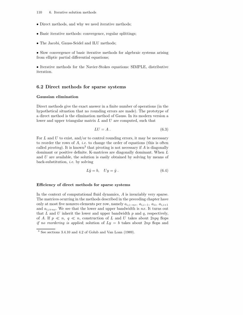
110 6. Iterative solution methods
• Direct methods, and why we need iterative methods;
• Basic iterative methods: convergence, regular splittings;
• The Jacobi, Gauss-Seidel and ILU methods;
• Slow convergence of basic iterative methods for algebraic systems arisingfrom elliptic partial differential equations;
• Iterative methods for the Navier-Stokes equations: SIMPLE, distributiveiteration.
6.2 Direct methods for sparse systems
Gaussian elimination
Direct methods give the exact answer in a finite number of operations (in thehypothetical situation that no rounding errors are made). The prototype ofa direct method is the elimination method of Gauss. In its modern version alower and upper triangular matrix L and U are computed, such that
LU = A . (6.3)
For L and U to exist, and/or to control rounding errors, it may be necessaryto reorder the rows of A, i.e. to change the order of equations (this is oftencalled pivoting). It is known3 that pivoting is not necessary if A is diagonallydominant or positive definite. K-matrices are diagonally dominant. When Land U are available, the solution is easily obtained by solving by means ofback-substitution, i.e. by solving
Ly = b, Uy = y . (6.4)
Efficiency of direct methods for sparse systems
In the context of computational fluid dynamics, A is invariably very sparse.The matrices ocurring in the methods described in the preceding chapter haveonly at most five nonzero elements per row, namely ai,i−nx, ai,i−1, aii, ai,i+1
and ai,i+nx. We see that the lower and upper bandwidth is nx. It turns outthat L and U inherit the lower and upper bandwidth p and q, respectively,of A. If p ≪ n, q ≪ n, construction of L and U takes about 2npq flopsif no reordering is applied; solution of Ly = b takes about 2np flops and
3 See sections 3.4.10 and 4.2 of Golub and Van Loan (1989).
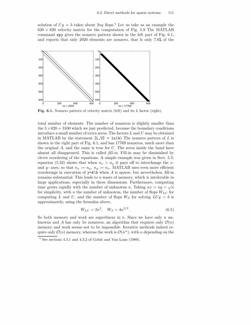
6.2 Direct methods for sparse systems 111
solution of Uy = b takes about 2nq flops.4 Let us take as an example the620 × 620 velocity matrix for the computation of Fig. 5.9 The MATLABcommand spy gives the nonzero pattern shown in the left part of Fig. 6.1,and reports that only 2920 elements are nonzero, that is only 7.6% of the
0 200 400 600
0
100
200
300
400
500
600
nz = 29200 200 400 600
0
100
200
300
400
500
600
nz = 17769
Fig. 6.1. Nonzero pattern of velocity matrix (left) and its L factor (right).
total number of elements. The number of nonzeros is slightly smaller thanthe 5×620 = 3100 which we just predicted, because the boundary conditionsintroduce a small number of extra zeros. The factors L and U may be obtainedin MATLAB by the statement [L,U] = lu(A) The nonzero pattern of L isshown in the right part of Fig. 6.1, and has 17769 nonzeros, much more thanthe original A, and the same is true for U . The zeros inside the band havealmost all disappeared. This is called fill-in. Fill-in may be diminished byclever reordering of the equations. A simple example was given in Sect. 5.5:equation (5.32) shows that when nx > ny it pays off to interchange the x-and y- axes, so that nx := ny, ny := nx. MATLAB uses even more efficientreorderings in execution of y=A\b when A is sparse, but nevertheless, fill-inremains substantial. This leads to a waste of memory, which is intolerable inlarge applications, especially in three dimensions. Furthermore, computingtime grows rapidly with the number of unknowns n. Taking nx = ny =
√n
for simplicity, with n the number of unknowns, the number of flops WLU forcomputing L and U , and the number of flops WS for solving LUy = b isapproximately, using the formulas above,
WLU = 2n2, WS = 4n3/2 . (6.5)
So both memory and work are superlinear in n. Since we have only n un-knowns and A has only 5n nonzeros, an algorithm that requires only O(n)memory and work seems not to be impossible. Iterative methods indeed re-quire only O(n) memory, whereas the work is O(nα), with α depending on the
4 See sections 4.3.1 and 4.3.2 of Golub and Van Loan (1989).

112 6. Iterative solution methods
method. Multigrid methods achieve the ideal value α = 1. For these efficiencyreasons, direct methods are seldom used in practical CFD. The remainder ofthis chapter is devoted to iterative methods. But first we will investigate whatcan be done with direct solution of the stationary Navier-Stokes equations.
Direct solution of the stationary Navier-Stokes equations
In the stationary case, the discretized form of the Navier–Stokes equationsfollows from equation (5.16) as
N(w) +Gp = f, Dw = g ,
where the algebraic vector that contains all velocity unknowns is now calledw. In order to apply a direct method for linear algebraic systems, we haveto linearize N(w) around an approximation wk−1 known from a precedingiteration. Let us use Picard linearization, as described in Sect. 5.4, and againin Sect. 6.4. This results in
N(w) ∼= Ck−1w ,
where Ck−1 is a matrix that depends on wk−1. The following iterative methodis obtained (Picard iteration):
Step 1. k = 0; choose wk.
Step 2. Generate Ck and solve the following linear system:
[
Ck GD 0
] [
wk+1
pk+1
]
=
[
fg
]
. (6.6)
Step 3. k = k + 1; go back to step 2; repeat until convergence criterion issatisfied.
Although we use (Picard) iteration, we will call this a direct method, becauseequation 6.6 is solved by a direct method. The method has been implementedin the MATLAB code ns3. In this code the algebraic vector w is partionedas
w =
[
uv
]
,
where u and v contain the horizontal and vertical velocity components. Thepartitioned system to be solved in step 2 now takes the following form:
Cku 0 Gu
0 Ckv Gv
Du Dv 0
uk+1
vk+1
pk+1
=
fu
fv
g
. (6.7)

6.2 Direct methods for sparse systems 113
This system is easily solved directly in MATLAB by the statement y=A\b,with appropriate definition of A, b and y.
Driven cavity flow
We now apply the above direct method to the flow in a driven cavity. Thedomain is the unit square surrounded by solid walls. The top wall is sliding tothe right with a velocity of magnitude 1. Fig. 6.2 shows the sparsity pattern
0 100 200 300
0
50
100
150
200
250
300
nz = 1664
Fig. 6.2. Sparsity pattern of matrix in equation (6.7), 10 × 10 grid.
of the matrix in equation (6.6). The 3 × 3 block partioning of the matrix inequation (6.7) is clearly visible. Fig. 6.3 shows a result. The computational
0 0.2 0.4 0.6 0.8 10
0.2
0.4
0.6
0.8
1Streamlines
0 10 20 30 4010
−5
10−4
10−3
10−2
10−1
100
Relative change per iteration
Fig. 6.3. Streamlines and convergence history for driven cavity problem, code ns3.Re = 5000, nx = ny = 64, nonuniform grid, central scheme.
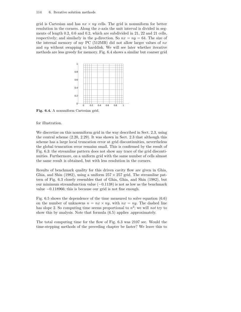
114 6. Iterative solution methods
grid is Cartesian and has nx × ny cells. The grid is nonuniform for betterresolution in the corners. Along the x-axis the unit interval is divided in seg-ments of length 0.2, 0.6 and 0.2, which are subdivided in 21, 22 and 21 cells,respectively; and similarly in the y-direction. So nx = ny = 64. The size ofthe internal memory of my PC (512MB) did not allow larger values of nxand ny without swapping to harddisk. We will see later whether iterativemethods are less greedy for memory. Fig. 6.4 shows a similar but coarser grid
0 0.2 0.4 0.6 0.8 10
0.2
0.4
0.6
0.8
1
Fig. 6.4. A nonuniform Cartesian grid.
for illustration.
We discretize on this nonuniform grid in the way described in Sect. 2.3, usingthe central scheme (2.20, 2.29). It was shown in Sect. 2.3 that although thisscheme has a large local truncation error at grid discontinuities, neverthelessthe global truncation error remains small. This is confirmed by the result ofFig. 6.3: the streamline pattern does not show any trace of the grid disconti-nuities. Furthermore, on a uniform grid with the same number of cells almostthe same result is obtained, but with less resolution in the corners.
Results of benchmark quality for this driven cavity flow are given in Ghia,Ghia, and Shin (1982), using a uniform 257 × 257 grid. The streamline pat-tern of Fig. 6.3 closely resembles that of Ghia, Ghia, and Shin (1982), butour minimum streamfunction value (−0.1138) is not as low as the benchmarkvalue −0.118966; this is because our grid is not fine enough.
Fig. 6.5 shows the dependence of the time measured to solve equation (6.6)on the number of unknowns n = nx × ny, with nx = ny. The dashed linehas slope 2. So computing time seems proportional to n2; we will not try toshow this by analysis. Note that formula (6.5) applies .approximately.
The total computing time for the flow of Fig. 6.3 was 2107 sec. Would thetime-stepping methods of the preceding chapter be faster? We leave this to
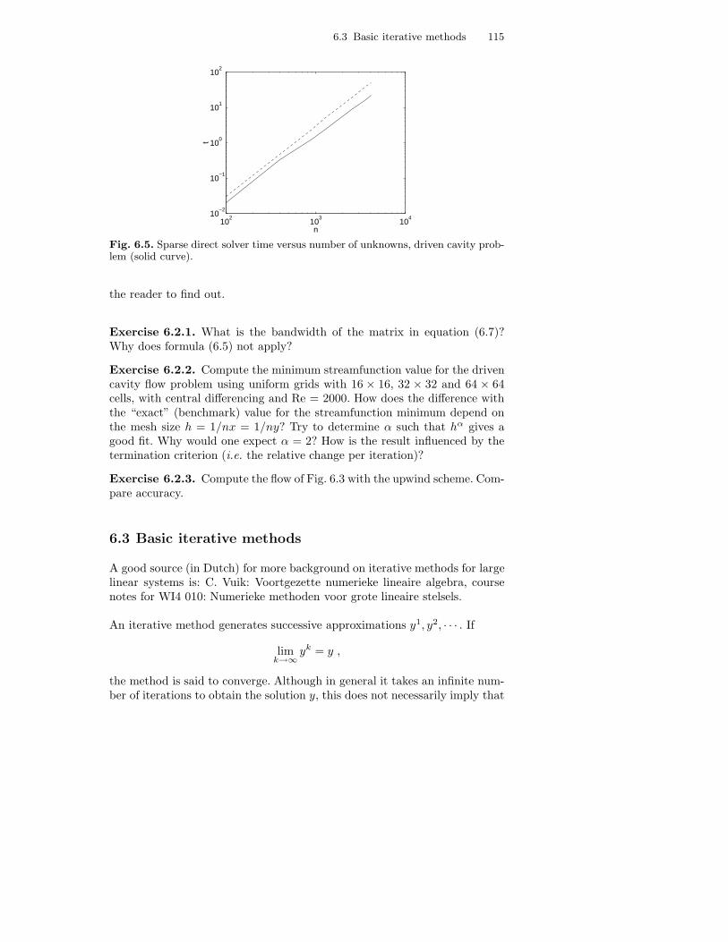
6.3 Basic iterative methods 115
102
103
104
10−2
10−1
100
101
102
n
t
Fig. 6.5. Sparse direct solver time versus number of unknowns, driven cavity prob-lem (solid curve).
the reader to find out.
Exercise 6.2.1. What is the bandwidth of the matrix in equation (6.7)?Why does formula (6.5) not apply?
Exercise 6.2.2. Compute the minimum streamfunction value for the drivencavity flow problem using uniform grids with 16 × 16, 32 × 32 and 64 × 64cells, with central differencing and Re = 2000. How does the difference withthe “exact” (benchmark) value for the streamfunction minimum depend onthe mesh size h = 1/nx = 1/ny? Try to determine α such that hα gives agood fit. Why would one expect α = 2? How is the result influenced by thetermination criterion (i.e. the relative change per iteration)?
Exercise 6.2.3. Compute the flow of Fig. 6.3 with the upwind scheme. Com-pare accuracy.
6.3 Basic iterative methods
A good source (in Dutch) for more background on iterative methods for largelinear systems is: C. Vuik: Voortgezette numerieke lineaire algebra, coursenotes for WI4 010: Numerieke methoden voor grote lineaire stelsels.
An iterative method generates successive approximations y1, y2, · · · . If
limk→∞
yk = y ,
the method is said to converge. Although in general it takes an infinite num-ber of iterations to obtain the solution y, this does not necessarily imply that
116 6. Iterative solution methods
iterative methods are less efficient than direct methods, because only a suffi-ciently accurate approximation to y is required. This is because y itself is anapproximation, which differs by the global truncation error from the exactsolution of the partial differential equation, of which the system to be solvedAy = b is a discrete approximation. Hence, a finite number of iterations suf-fices.
Let us consider only stationary iterative methods; that is, methods in whichthe same algorithm is applied in every iteration. Let, furthermore, the com-putation of the new iterand yk involve only matrix multiplication and vectoraddition:
yk = Byk−1 + c , (6.8)
where the matrix B and the vector c remain to be chosen. For yk to con-verge to the solution y = A−1b it is obviously necessary that y is a stationarypoint of the iteration process (6.8), i.e. y = By + c, hence we must havec = (I −B)A−1b, so that (6.8) can be rewritten as
Myk = Nyk−1 + b, M −N = A . (6.9)
(We have M −N = A because M = A(I −B)−1, N = MB). Equation (6.9)can be rewritten in the following equally useful form:
Mδy = b−Ayk−1, yk = yk−1 + δy. (6.10)
Application of underrelaxation or overrelaxation with relaxation parameter αmeans that (6.10) is replaced by
Mδy = α(b −Ayk−1), yk = yk−1 + δy. (6.11)
We will call methods of type (6.9) or (6.10) or (6.11) basic iterative methods,or BIMs for brevity.
Instead ofB one usually specifiesM . One can think ofM as an approximationof A; if M = A and α = 1 we have convergence in one iteration. We have(the reader should check this)
B = I −M−1A .
The error ek ≡ y − yk satisfies ek = Bek−1, so that convergence is governedby B, which is called the iteration matrix. Since ek = Bke0 (where of coursethe superscript k on B is not an index but an exponent),
‖ek‖ ≤ ‖Bk‖ ‖e0‖ . (6.12)
From equation (6.2) it follows that we have convergence (‖ek‖ → 0) if andonly if
ρ(B) < 1 . (6.13)

6.3 Basic iterative methods 117
When to stop?
For efficiency, which is what iterative methods are all about, it is necessaryto stop iterating as soon as sufficient precision has been obtained. Hence,we need a good termination criterion. The difference between two successiveiterates usually does not give a good indication of the precision achieved. Thiscan be seen as follows. Let B have a single dominating real eigenvalue λ =ρ(B), with corresponding eigenvector x. Then we have after many iterationsek ∼= αλkx, with α some constant. It follows that
yk+1 − yk ∼= αλk(λ − 1)x = (λ − 1)ek ,
so that
ek ∼= yk+1 − yk
λ− 1.
We see that if λ = 1−ǫ, 0 < ǫ≪ 1, as frequently happens (slow convergence),then the error is much larger than the difference between two successiveiterates. Therefore it is better to derive a termination criterion from theresidual rk ≡ b−Ayk. After k iterations we have solved exactly the followingapproximate problem:
Ayk = b− rk .
Frequently, perturbation of the right-hand side has a physical interpretation,or b is known to have an error with a known bound, which enables one todecide what size of ‖rk‖ is tolerable.
Why it is nice if A is a K-matrix
In sections 2.3 and 3.3 we saw that if the scheme Lh is of positive type, thenit satisfies a maximum principle, so that unphysical oscillations (wiggles) areexcluded. It is easy to see that if Lh is of positive type, then the correspondingmatrix is a K-matrix. The second reason why it is nice if A is a K-matrix is,that it is easy to devise convergent BIMs. This is shown below.
Regular splittings
We just saw that a BIM is defined by a specification of an approximation Mof A. How to choose M? Obviously, M must be such that equation (6.9) canbe solved efficiently. Furthermore, the method must be convergent: ρ(B) =ρ(I −M−1N) < 1. Finally, the BIM must converge rapidly. We will now seethat it is easy to devise convergent BIMs if A is an M-matrix, for example aK-matrix. The speed of convergence will be examined later.
Definition 6.3.1. The splitting A = M − N is called regular if M−1 ≥ 0and N ≥ 0. The splitting is called convergent if (6.9) converges.
118 6. Iterative solution methods
We have the following nice theorem:
Theorem 6.3.1. A regular splitting of an M -matrix is convergent.
Proof. See Theorem 3.13 in Varga (1962). 2
Hence, we aim for regular splittings. The following theorem shows that regularsplittings are easy to obtain for M-matrices:
Theorem 6.3.2. Let A be an M -matrix. If M is obtained by replacing someelements aij , j 6= i by bij satisfying aij ≤ bij ≤ 0, then A = M − N is aregular splitting.
Proof. See Theorem 7.2.6 in Wesseling (2001). 2
This means, for example, that if A is a K-matrix, and if we make M byreplacing arbitrary off-diagonal elements aij , i 6= j by 0, then we have aregular splitting (note that for if A is a K-matrix, then aij ≤ 0, i 6= j, sothat M will be a K-matrix, and N ≥ 0). This gives us great freedom indesigning regular splittings.
Examples
Jacobi
The Jacobi method is obtained by taking M = D ≡ diag(A). This gives thefollowing BIM:
Dyk = (D −A)yk−1 + b .
Gauss-Seidel
The Gauss-Seidel method is obtained as follows. Write A = D − E − F ,with D = diag(A), E strictly lower triangular (i.e. Eij = 0, j ≥ i) and Fstrictly upper triangular (E is simply the strictly lower triangular part of−A, and F the upper part of −A). We take M = D − E (forward Gauss-Seidel) or M = D − F (backward Gauss-Seidel). With this M it is also easyto solve for yk, because M is lower or upper triangular; yk is obtained byback-substitution. For example, forward Gauss-Seidel can be written as
yki =
bi −i−1∑
j=1
aijykj −
n∑
j=i+1
aijyk−1j
/aii .
ILU
Unlike the preceding two methods, the incomplete LU (ILU) method is notobtained by replacing elements of A by zero. The idea is to determine lowerand upper tridiagonal matrices L and U such that LU ∼= A, and to chooseM = LU . If LU = A we get N = 0, and we are back at the direct (Gaussianelimination) method described before. But the difference is that the cause of

6.3 Basic iterative methods 119
the inefficiency is eliminated by forbidding fill-in; hence, LU 6= A, but thehope is that LU will not be far from A, so that we have rapid convergence.ILU decomposition works as follows. The elements of L and U are prescribedto be zero, except if (i, j) ∈ Q, where Q is the set of index pairs where weallow nonzeros:
Q ⊂ Qn, Qn ≡ (i, j), 1 ≤ i ≤ n, 1 ≤ j ≤ n .
An example of a suitable set Q will follow. ILU is based on the followingtheorem:
Theorem 6.3.3. Let A be an M-matrix. Then for every Q ⊂ Qn there exista lower triangular matrix L with lii = 1, an upper triangular matrix U anda matrix N ≥ 0 such that A = LU −N and
lij = 0 and uij = 0 if (i, j) 6∈ Q ,
nij = 0 if (i, j) ∈ Q .
Furthermore, the iterations LUyk = b+Nyk−1 converge.
Proof. See Meijerink and van der Vorst (1977). 2
Again we see that the M-matrix property is crucial.
We have(LU)ij = aij , (i, j) ∈ Q ,
but we can have (LU)ij 6= aij , (i, j) 6∈ Q. The so-called first order ILUdecomposition is obtained by choosing Q equal to the nonzero pattern of A.For instance, if the scheme Lh has the following five point stencil:
[Lh] =
∗∗ ∗ ∗
∗
, (6.14)
then the nonzero pattern QA of A is, with lexicographic ordering
QA = i, j ∈ Qn, j = i or j = i± 1 or j = i± nx .
It comes as a nice surprise that the nonzero pattern of N = LU − A turnsout to be very small:
QN = i, j ∈ Qn, j = i+ nx− 1 or j = i− nx+ 1 .
So N has only two nonzero diagonals. We hope the elements will be small,because the closer M = LU is to A, the faster convergence will be.
120 6. Iterative solution methods
Incomplete Cholesky decomposition
If a matrix A is symmetric and positive definite, then it has not only an LUdecomposition, but also a Cholesky decomposition:
LLT = A
with now diag(L) 6= I. An advantage is that there is no need to store U .Similarly to ILU, there exist incomplete Cholesky decompositions (ICs). Wenow present an algorithm to compute an IC. Let the matrix A (symmetric,of course) be a discretization on an n × n or n × n × n grid, so the size ofA is either n2 × n2 or n3 × n3. It is convenient to temporarily write the ICdecomposition as LD−1LT with diag(L) = D. We want to make a first orderIC. This means that lij 6= 0 only if aij 6= 0. We choose lij = aij , i 6= j. Inthe two-dimensional case, let A correspond to the stencil (6.14), so that thenonzero elements are aii, ai,i±1, ai,i±n. If we define
dii = aii − a2i,i−1/di−1,i−1 − a2
i,i−n/di−n,i−n , (6.15)
where term with an index < 1 are to be deleted, then we have
(LD−1LT )ij = aij , if aij 6= 0 . (6.16)
It is left to the reader to verify this. Similarly, in three dimensions:
dii = aii − a2i,i−1/di−1,i−1 − a2
i,i−n/di−n,i−n − a2i,i−n2/di−n2,i−n2 . (6.17)
Finally, we bring the IC in the form LLT by defining
L := LD−1/2 ,
where D−1/2 = diag(d−1/2). Equations (6.15) and (6.17) have been imple-mented, for the model problem described below, in the MATLAB M-filemy_cholinc, because MATLAB’s cholinc is inefficient.
A model problem
Let us consider the Poisson equation on the unit square with a homogeneousDirichlet boundary condition:
−ϕxx − ϕyy = f(x, y), (x, y) ∈ Ω ≡ (0, 1) × (0, 1), ϕ|∂Ω = 0 . (6.18)
We discretize on a homogeneous (n+ 2) × (n+ 2) vertex-centered grid suchas shown in Fig. 6.6. We index only the interior points with i, j = 1, · · · , n,so n = 2 in Fig. 6.6. Standard finite difference or finite volume discretizationof (6.18) gives
Lhϕij ≡ 4ϕij − ϕi−1,j − ϕi+1,j − ϕi,j−1 − ϕi,j+1 = h2fij , i, j = 1, · · · , n ,(6.19)
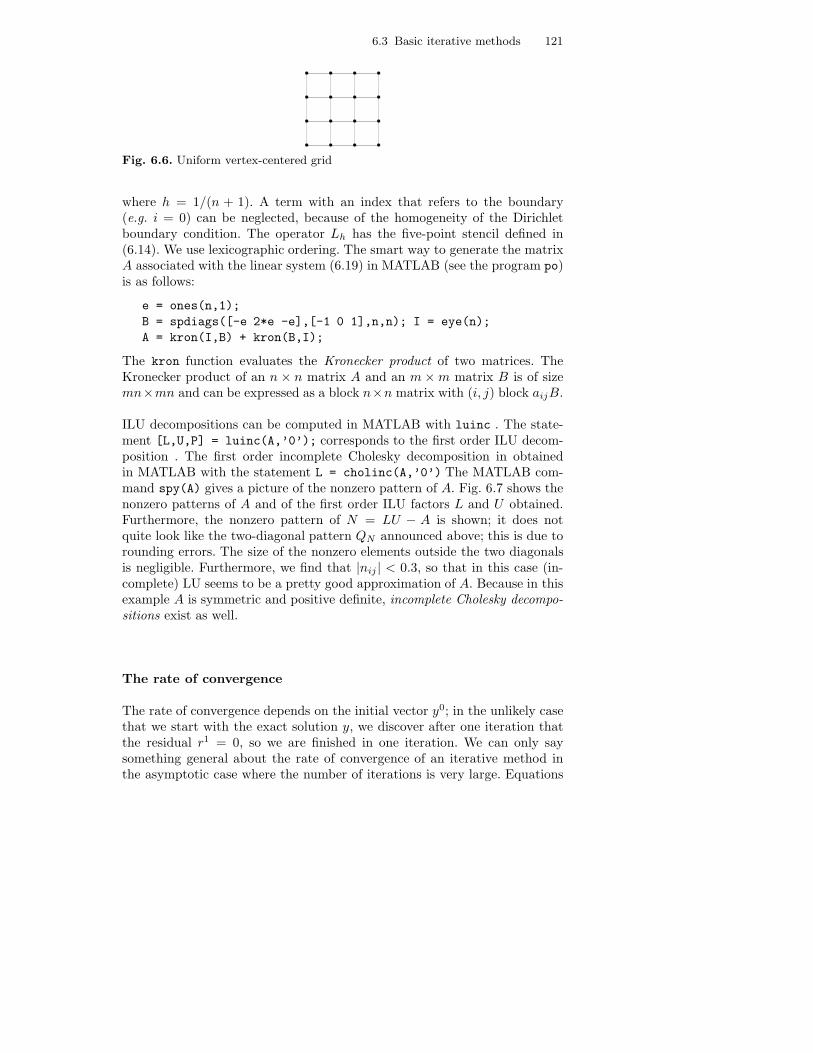
6.3 Basic iterative methods 121
Fig. 6.6. Uniform vertex-centered grid
where h = 1/(n + 1). A term with an index that refers to the boundary(e.g. i = 0) can be neglected, because of the homogeneity of the Dirichletboundary condition. The operator Lh has the five-point stencil defined in(6.14). We use lexicographic ordering. The smart way to generate the matrixA associated with the linear system (6.19) in MATLAB (see the program po)is as follows:
e = ones(n,1);
B = spdiags([-e 2*e -e],[-1 0 1],n,n); I = eye(n);
A = kron(I,B) + kron(B,I);
The kron function evaluates the Kronecker product of two matrices. TheKronecker product of an n × n matrix A and an m×m matrix B is of sizemn×mn and can be expressed as a block n×n matrix with (i, j) block aijB.
ILU decompositions can be computed in MATLAB with luinc . The state-ment [L,U,P] = luinc(A,’0’); corresponds to the first order ILU decom-position . The first order incomplete Cholesky decomposition in obtainedin MATLAB with the statement L = cholinc(A,’0’) The MATLAB com-mand spy(A) gives a picture of the nonzero pattern of A. Fig. 6.7 shows thenonzero patterns of A and of the first order ILU factors L and U obtained.Furthermore, the nonzero pattern of N = LU − A is shown; it does notquite look like the two-diagonal pattern QN announced above; this is due torounding errors. The size of the nonzero elements outside the two diagonalsis negligible. Furthermore, we find that |nij | < 0.3, so that in this case (in-complete) LU seems to be a pretty good approximation of A. Because in thisexample A is symmetric and positive definite, incomplete Cholesky decompo-sitions exist as well.
The rate of convergence
The rate of convergence depends on the initial vector y0; in the unlikely casethat we start with the exact solution y, we discover after one iteration thatthe residual r1 = 0, so we are finished in one iteration. We can only saysomething general about the rate of convergence of an iterative method inthe asymptotic case where the number of iterations is very large. Equations

122 6. Iterative solution methods
0 5 10 15 20 25 30 35
0
5
10
15
20
25
30
35
nz = 1560 5 10 15 20 25 30 35
0
5
10
15
20
25
30
35
nz = 96
0 5 10 15 20 25 30 35
0
5
10
15
20
25
30
35
nz = 960 5 10 15 20 25 30 35
0
5
10
15
20
25
30
35
nz = 65
Fig. 6.7. Nonzero patterns of A, of ILU factors L and U , and of N ≡ LU −A; firstorder ILU decomposition.
(6.2) and (6.12) show that for k ≫ 1 the error ek = y − yk satisfies
‖ek‖ ≤ ρ(B)‖ek−1‖, B = I −M−1A . (6.20)
So the quality measure of a BIM is its spectral radius ρ(B): the smaller ρ(B),the better (of course, the computing work per iteration should also be takeninto account). However, in general, ρ(B) is not easy to determine. We willdo this for an illustrative example, namely the Poisson problem introducedabove. Analysis is easier in the difference form than in the matrix form. TheJacobi method applied to the scheme (6.19) gives:
4ϕk+1ij = ϕk
i−1,j + ϕki+1,j + ϕk
i,j−1 + ϕki,j+1 + h2fij , i, j = 1, · · · , n . (6.21)
Here and in what follows terms with i or j 6∈ 1, · · · , n are defined to bezero. The exact solution ϕij satisfies (6.21). Subtraction gives for the errorek
ij = ϕij − ϕkij :
ek+1 = Bek, Beij ≡ (ei−1,j + ei+1,j + ei,j−1 + ei,j+1)/4 , (6.22)
6.3 Basic iterative methods 123
together with the boundary condition e0,j = en+1,j = ei,0 = ei,n+1 = 0. Ourpredecessors have found out that the eigenfunctions of the operator B are:
ψij = sin iphπ sin jqhπ, h = 1/(n+ 1), p, q ∈ 1, · · · , n , (6.23)
which is easily verified by inspection: substitution of (6.23) in (6.22) gives
Bψ = λψ, λ =1
2(cos phπ + cos qhπ) , (6.24)
where one needs the trigonometric identity
sinα+ sinβ = 2 sin1
2(α+ β) cos
1
2(α− β) .
Clearly, we have found n2 independent eigenfunctions (or eigenvectors) ψ,since each pair p, q admitted by (6.23) gives us an eigenfunction. Since Bcorresponds to an n2 × n2 matrix, we have found all its eigenvectors; hence,(6.24) gives us all eigenvalues. The maximum |λ| delivers the spectral radius:
ρ(B) = cosπh . (6.25)
Hence,ρ(B) ∼= 1 −O(h2) . (6.26)
Equation (6.26) turns out to be true in general for BIMs applied to numeri-cal schemes for second order elliptic partial differential equations on generalgrids with mesh size proportional to h.
How many iterations are required to have an error reduction of 10−d, i.e. togain d decimal digits? According to equations (6.12) and (6.2), we must haveρ(B)k < 10−d, hence k ln ρ(B) < −d ln 10, or
k > −d ln 10/ lnρ(B) .
We have (cf. Exercise 6.3.5)
ln ρ(B) ∼= −1
2(πh)2 ,
hence the number of iterations required m satisfies
m ∼= 2d ln 10
π2N .
where N ∼= 1/h2 temporarily stands for the total number of unknowns. From(6.21) it follows that a Jacobi iteration takes 5N flops, so the total workWJ = 5Nm satisfies
WJ = O(N2) . (6.27)

124 6. Iterative solution methods
As seen before, direct methods also have W = O(N2), so the Jacobi method(and other BIMs) do not bring us closer to the ideal W = O(N), althoughGauss-Seidel converges twice as fast than Jacobi, see Exercise 6.3.8 (this isnot surprising, because Gauss-Seidel uses updated variables as soon as theybecome available). BIMs only bring a saving in computer memory.
Exercise 6.3.1. Derive equation (6.10) from equation (6.9).
Exercise 6.3.2. Express the iteration matrix B in terms of M and A in thecase that relaxation with parameter α is applied.
Exercise 6.3.3. Verify equation (6.16).
Exercise 6.3.4. Verify equation (6.24).
Exercise 6.3.5. Show that if |ε| ≪ 1
ln cos ε ∼= −1
2ε2 .
Exercise 6.3.6. Show that if A is an M-matrix, then Jacobi and Gauss-Seidel correspond to regular splittings. Why is this nice?
Exercise 6.3.7. Write down the Gauss-Seidel variants (forward and back-ward) of equation (6.21).
Exercise 6.3.8. It is known5 that, for matrices generated by discretizationson the type of grid considered in these lecture notes, the spectral radii of theGauss-Seidel and Jacobi methods are related by
ρ(BGS) = ρ(BJ)2 .
Show that Gauss-Seidel requires half as much computing work as Jacobi.
6.4 Krylov subspace methods
Acceleration of basic iterative methods
So why bother with BIMs? The answer is: BIMs are essential as indispensablebuilding blocks inside more complicated but very efficient methods.
To begin with, BIMs can be accelerated by Krylov subspace methods. Thismeans that we take a BIM, corresponding to a splitting A = M − N , and
5 See Corollary 2.3 in Chapt. 5 in Young (1971)
6.4 Krylov subspace methods 125
use M to precondition the problem to be solved Ay = b, which means thatAy = b is replaced by its preconditioned version:
M−1Ay = M−1b . (6.28)
We call M a good preconditioner if (6.28) lends itself well for efficient solu-tion by Krylov subspace methods. Therefore an iterative method is frequentlycalled a preconditioner. One may say that convergence of the BIM is ac-celerated by a Krylov subspace method, or that convergence of the Krylovsubspace method is accelerated by the BIM.
Secondly, BIMs can be accelerated by multigrid methods. We call a BIMa good smoother if the BIM makes the error rapidly smooth (although notrapidly small). Then the error can be made rapidly small with a multigridmethod. In principle this approach leads to the ideal efficiency
Work = O(N)
with N the total number of unknowns.
We have no time in this course to explain the principles of Krylov subspaceand multigrid methods, but will show how Krylov subspace methods thathave been implemented in MATLAB can be used.
Preconditioned conjugate gradients
The conjugate gradients (CG) method is a particular Krylov subspace methodfor linear systems Ay = b with a symmetric positive definite matrix A. It iscalled in MATLAB by
y = pcg(A,b,tol,maxit)
with maxit the maximum number of iterations allowed, and tol the relativeerror in the residual, defined by
‖Ay − b‖‖b‖ .
For information on Krylov subspace methods for nonsymmetric A that havebeen implemented in MATLAB, type: help pcg , and call help for thefunctions listed under “See also”.
It is known6 that the number of iterations required by CG is proportionalto
√cond(A). To make cond(A) smaller, the system is preconditioned, as in
6 This follows from Theorem 10.2.5 in Golub and Van Loan (1989)
126 6. Iterative solution methods
equation (6.28). Because the preconditioned matrix must be symmetric inorder to apply CG, we choose the preconditioned system as follows:
L−1AL−T y = L−1b, y = L−T y , (6.29)
where LLT is an incomplete Cholesky decomposition of A, and L−T =(LT )−1. If CG is applied with incomplete Cholesky preconditioning, the re-sulting method is called ICCG (incomplete Cholesky conjugate gradients).
We will now determine the condition number of A for our model problem(6.19). We have A = 4(I − B), with B given in equation (6.22). If p(x) is apolynomial, then λ(p(A)) = p(λ(A)). Hence, λ(A) = 4 − 4λ(B), so that
λ(A) = 4(
sin2 12pπh+ sin2 1
2qπh)
, p, q = 1, · · · , n, h = 1/(n+ 1) ,
hence
min |λ(A)| = 8 sin2 π/2(n+ 1), max |λ(A)| = 8 sin2 nπ/2(n+ 1) ,
For
cond(A) ≡ max |λ(A)|min |λ(A)|
we find, taking n = 50:
cond(A) = 1.0535e+ 03
We can also estimate cond(A) with MATLAB. By running powith dim = 2 andn = 50 and typing condest(A) we find:
cond(A) = 1.5315e+ 03 ,
which is not very accurate but gives the right size. By typing
B=inv(L)*A*inv(L’);
cond(B)
we findcond(L−1AL−T ) = 221 .
This reduction in condition number that IC preconditioning brings is whatmakes ICCG a great succes; the reduction factor grows with n.
The following MATLAB code is an implementation of ICCG:
L = cholinc(A,’0’); % First order IC decomposition
y = pcg(A,b,1e-2,200,L’,L); % Preconditioned cg method
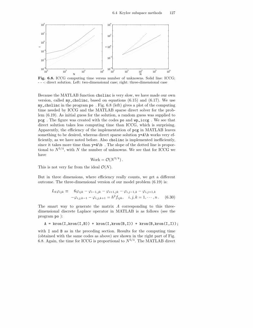
6.4 Krylov subspace methods 127
102
103
104
105
10−3
10−2
10−1
100
101
102
N
t
102
103
104
105
106
10−4
10−2
100
102
104
N
t
Fig. 6.8. ICCG computing time versus number of unknowns. Solid line: ICCG;- - -: direct solution. Left: two-dimensional case; right: three-dimensional case
Because the MATLAB function cholinc is very slow, we have made our ownversion, called my_cholinc, based on equations (6.15) and (6.17). We usemy_cholinc in the program po . Fig. 6.8 (left) gives a plot of the computingtime needed by ICCG and the MATLAB sparse direct solver for the prob-lem (6.19). As initial guess for the solution, a random guess was supplied topcg . The figure was created with the codes po and wp_iccg . We see thatdirect solution takes less computing time than ICCG, which is surprising.Apparently, the efficiency of the implementation of pcg in MATLAB leavessomething to be desired, whereas direct sparse solution y=A\b works very ef-ficiently, as we have noted before. Also cholinc is implemented inefficiently,since it takes more time than y=A\b . The slope of the dotted line is propor-tional to N5/4, with N the number of unknowns. We see that for ICCG wehave
Work = O(N5/4) .
This is not very far from the ideal O(N).
But in three dimensions, where efficiency really counts, we get a differentoutcome. The three-dimensional version of our model problem (6.19) is:
Lhϕijk ≡ 6ϕijk − ϕi−1,jk − ϕi+1,jk − ϕi,j−1,k − ϕi,j+1,k
−ϕi,j,k−1 − ϕi,j,k+1 = h2fijk, i, j, k = 1, · · · , n . (6.30)
The smart way to generate the matrix A corresponding to this three-dimensional discrete Laplace operator in MATLAB is as follows (see theprogram po ):
A = kron(I,kron(I,B)) + kron(I,kron(B,I)) + kron(B,kron(I,I));
with I and B as in the preceding section. Results for the computing time(obtained with the same codes as above) are shown in the right part of Fig.6.8. Again, the time for ICCG is proportional to N5/4. The MATLAB direct
128 6. Iterative solution methods
solver is now much less efficient. This illustrates that in three dimensionsiterative methods are indispensable.
Exercise 6.4.1. Show that the matrix L−1AL−T in equation (6.29) is sym-metric positive definite if A is symmetric positive definite.
Exercise 6.4.2. Show that if p(x) is a polynomial, then λ(p(A)) = p(λ(A)).
Exercise 6.4.3. Compare the efficiency of unpreconditioned and precondi-tioned CG by suitably modifying and running the program po
6.5 Distributive iteration
We will now apply basic iterative methods to the stationary Navier-Stokesequations. The discretized stationary Navier-Stokes equations are obtainedfrom equation (5.16) in the following form:
N(u) +Gp = f, Du = g , (6.31)
with N a nonlinear algebraic operator. This nonlinear system has to be solvediteratively. We use Picard iteration, as decribed in Sect. 5.4. This works asfollows. Let superscript k be the iteration counter. Then, for example, termslike u2
jk and (uv)j+1/2,k+1/2 (with u and v now temporarily denoting thetwo velocity components) in the discretized x-momentum equation (5.11) arereplaced by
u2jk
∼= (uk−1uk)jk, (uv)j+1/2,k+1/2∼= (ukvk−1)j+1/2,k+1/2 .
As a consequence (using u again to denote the algebraic vector containingall velocity unknowns), N(u) gets replaced by Ck−1uk, with Ck−1 a matrixthat depends on uk−1. The system (6.31) now can be written as:
[
Ck−1 GD 0
] [
uk
pk
]
=
[
fg
]
. (6.32)
Picard iteration works as follows:
Step 1. k = 0. Choose u0, p0.Step 2. k = k + 1. Generate the matrix Ck−1.Step 3. Solve equation (6.32).Step 4. Return to step 2. Repeat until convergence criterion is satisfied.
The block-partioned matrix in (6.32) is not a K-matrix and also not an M-matrix, because of the zero block on the main diagonal. So we cannot obtain aregular splitting. In other words, it is not trivial to design a simple convergentiterative method.
6.5 Distributive iteration 129
The SIMPLE method
In 1972 an iterative method was proposed by Patankar and Spalding, whichthey called the SIMPLE method (SIMPLE stands for semi-implicit methodfor pressure-linked equations). With SIMPLE we do not solve equation (6.32)accurately, but perform only one iteration step. SIMPLE consists of the fol-lowing steps:
Step 1. k = 0. Choose u0, p0.Step 2. k = k + 1. Generate the matrix Ck−1.Step 3. Update u by an approximate solve of the first row of (6.32):
Ck−1uk = f −Gpk−1 ,
using a splitting Mu−Nu = Ck−1 of Ck−1, that is regular if C is a K-matrix,which is the case if the mesh Reynolds number is less than 2 or if we use theupwind scheme for the inertia terms; see Sect. 2.3 (equation (2.41)). Hence,if we would execute this step repeatedly it would converge. But we do onlyone iteration and then improve the pressure in step 4. We use the BIM in theform (6.11):
1
αuMuδu = f − Ck−1uk−1 −Gpk−1, uk = uk−1 + δu ,
where αu is an underrelaxation factor that, unfortunately, must be deter-mined by trial and error; αu = 0.5 seems to be a suitable value.
Step 4. Update p by an approximate solve of the following equation:
DC−1Gδp = Duk , (6.33)
where C ≡ diag(Ck−1). At first sight, the motivation for equation (6.33)seems unclear; it is inspired by the pressure-correction method, and is furtherjustified below. It turns out that DC−1G is a K-matrix. So we use a splittingMp −Np = DC−1G. By employing the underrelaxed BIM formulation (6.11)we obtain :
1
αpMpδp = Duk, pk = pk−1 + δp .
where the underrelaxation factor αp must, unfortunately, be determined bytrial and error; αp = 0.8 seems to be a suitable value.
Step 5. Second velocity update:
uk := uk − C−1Gδp .
Step 6. k := k + 1, and return to step 2. Repeat until convergence criterionis satisfied.

130 6. Iterative solution methods
Distributive iteration
It is clear that upon convergence, when we have uk = uk−1 and δp = 0, wehave indeed solved equation (6.28). But does SIMPLE converge? To see thisit is convenient to take a modern point of view, and to regard SIMPLE asa member of the class of distributive iteration methods. This framework alsomakes equation (6.33) more understandable. The idea is as follows.Suppose we have a linear system Ay = b. The system is postconditioned:
ABy = b, y = By . (6.34)
The postconditioning matrix B is chosen such that (6.34) is easier to solveiteratively than Ay = b. For example, AB is an M-matrix, while A is not,as in our Navier-Stokes case above. For the iterative solution of (6.34) thesplitting
AB = M −N (6.35)
is introduced, to which corresponds the following splitting of the originalmatrix A:
A = MB−1 −NB−1 .
This leads to the following stationary iterative method for Ay = b:
MB−1yk+1 = NB−1yk + b ,
oryk+1 = yk +BM−1(b−Ayk) . (6.36)
This can be solved as follows:
Step 1. Solve Mδy = b −Ayk.Step 2. δy = Bδy.Step 3. yk+1 = yk + δy.
Note that if the iterative method defined by (6.36) converges (yk+1 = yk),it solves Ay = b. This means that when designing a distributive iterationmethod, B and M in (6.36) need not be precisely the same as in (6.35). Forexample, one could use a complicated B to design a good M for (6.35), withN small, and then changeM a little in (6.36) to make in step 1Mδy = b−Ayk
more easily solvable, and also B may be simplified to make (6.36) easy toapply.
The method (6.36) is called distributive iteration for the following reason.Equation (6.36) and step 2 show that the correction M−1(b − Ayk) corre-sponding to non-distributive (B = I) iteration is distributed, so to speak, bymultiplication with B, over the elements of yk+1, whence the name of themethod.
6.5 Distributive iteration 131
Distributive iteration for Navier-Stokes
A number of well-known iteration methods for the incompressible Navier-Stokes equations can be interpreted as distributive methods. The distributiveiteration framework permits us to give a unified description.
The system to be solved is (6.32). Define (writing C instead of Ck−1 forbrevity)
A =
[
C GD 0
]
. (6.37)
A possible choice for B is:
B =
[
I −C−1G0 I
]
, (6.38)
resulting in
AB =
[
C (I − CC−1)G
D −DC−1G
]
.
Note that the zero block on the main diagonal has disappeared (this is thepurpose of distributive iteration), so that basic iterative methods have achance to converge. It remains to specify a suitable approximation M of AB.Thinking of C as an approximation of C, we hope that I − CC−1 will besmall; this is the motivation behind equation (6.33). So we delete the block(I−CC−1)G. Furthermore, we replace C by Mu/αu of step 3 of the SIMPLEmethod and DC−1G by Mp/αp of step 4. This gives
M =
[
1αuMu 0
D − 1αpMp
]
. (6.39)
Substitution of (6.38) and (6.39) in (6.36) gives the following iterativemethod:
Step 1. Determine
[
rurp
]
=
[
fg
]
−[
C GD 0
] [
uk
pk
]
. (6.40)
Step 2. Solve[
1αuMu 0
D − 1αpMp
]
[
δuδp
]
=
[
rurp
]
. (6.41)
Step 3. Carry out the distribution step:
[
δuδp
]
:= B
[
δuδp
]
=
[
δu− C−1Gδpδp
]
. (6.42)

132 6. Iterative solution methods
This is completely equivalent to the SIMPLE method described earlier; thereader should verify this. By changing M and B different variants of theSIMPLE method that have appeared in the literature such as SIMPLER andSIMPLEC, and another distributive method called distributive Gauss-Seidelmay be obtained. So distributive iteration is a useful unifying framework.
Roughly speaking, SIMPLE does for Navier-Stokes what Jacobi and Gauss-Seidel do for the Poisson equation studied earlier. So convergence will be slowand the work will still be O(N2). But, like BIMs, SIMPLE lends itself well foracceleration by Krylov subspace methods and multigrid. We will not discussthis here. The interested reader is referred to Chapt. 7 of Wesseling (2001),and references given there.
When to stop SIMPLE iterations? The advice is to make the velocity fieldsufficiently divergence free, i.e. to make Duk suficiently small, for instance
‖ Duk ‖∞< tolU/L, tol ≪ 1 ,
where U and L are typical magnitudes for the velocity and the size of thedomain. The reason is that if in incompressible flows divu is not sufficientlysmall, we have numerical mass sources and sinks, which is usually very detri-mental for physical realism.
Final remark
As we have seen, basic iterative methods usually are very slow to converge. Aswe remarked before, they are very useful if they are accelerated with Krylovsubspace or multigrid methods. Unfortunately, in this course we have no timeto discuss these methods.
Exercise 6.5.1. Verify that the distributive and the original formulation ofthe SIMPLE method are equivalent.
Some self-test questions
How many flops does it take to solve a system Ay = b with A a symmetric n × n matrix withbandwidth 2m − 1, m ≪ n, with a direct method without reordering?
What is fill-in?
Describe the matrix structure of the linearized staggered scheme.
Describe the driven cavity benchmark problem.
What is a basic iterative method?
133
Give a good termination criterion for basic iterative methods.
What is a K-matrix? What is an M-matrix?
What is a regular splitting? What is the nice property of a regular splitting?
Describe the Jacobi, Gauss-Seidel, ILU and IC methods.
Let the iteration matrix of a BIM have spectral radius ρ < 1. How many iterations are equiredto reduce the error by a factor r?
Describe distributive iteration. Why is it useful for Navier-Stokes?

References
Aris, R. (1962). Vectors, Tensors and the Basic Equations of Fluid Me-chanics. Englewood Cliffs, N.J.: Prentice-Hall, Inc. Reprinted, Dover,New York, 1989.
Batchelor, G.K. (1967). An Introduction to Fluid Dynamics. Cambridge,UK: Cambridge University Press.
Burden, R.L. and J.D. Faires (2001). Numerical analysis. Pacific Grove:Brooks/Cole.
de Saint-Venant, B. (1843). Memoire sur la dynamique des fluides. C. R.Acad. Sci. Paris 17, 1240–1242.
Ghia, U., K.N. Ghia, and C.T. Shin (1982). High-Re solutions for in-compressible flow using the Navier-Stokes equations and a multigridmethod. J. Comp. Phys. 48, 387–411.
Golub, G.H. and C.F. Van Loan (1989). Matrix Computations (secondedition). Baltimore: The Johns Hopkins University Press.
Hackbusch, W. (1994). Iterative Solution of Large Sparse Systems Equa-tions. New York: Springer.
Hinze, J.O. (1975). Turbulence. New York: McGraw-Hill.Hirsch, C. (1988). Numerical Computation of Internal and External Flows.
Vol.1: Fundamentals of Numerical Discretization. Chichester: Wiley.Lighthill, J. (1986). The recently recognized failure of predictability in
Newtonian dynamics. Proc. R. Soc. London A407, 35–50.Meijerink, J.A. and H.A. van der Vorst (1977). An iterative solution
method for linear systems of which the coefficient matrix is a sym-metric M-matrix. Math. Comp. 31, 148–162.
Nakayama, Y. and W.A. Woods (Eds.) (1988). Visualized Flow; Fluid Mo-tion in Basic and Engineering Situations Revealed by Flow Visualiza-tion. Oxford: Pergamon.
Navier, C.L.M.H. (1823). Memoire sur les lois du mouvement des fluides.Mem. Acad. R. Sci. Paris 6, 389–416.
Poisson, S.D. (1831). Memoire sur les equations generales de l’equilibre etdu mouvement des corps solides elastiques et des fluides. Journal del’Ecole Polytechnique de Paris 13, 139–166.
136 REFERENCES
Stokes, G.G. (1845). On the theories of the internal friction of fluids inmotion, and of the equilibrium and motion of elastic solids. Trans.Camb. Phil. Soc. 8, 287–305.
Stokes, G.G. (1851). On the effect of the internal friction of fluids on themotion of pendulums. Trans. Camb. Phil. Soc. 9, Pt. II, 8–106.
Trottenberg, U., C.W. Oosterlee, and A. Schuller (2001). Multigrid. Lon-don: Academic Press.
Van Dyke, M. (1982). An Album of Fluid Motion. Stanford: The ParabolicPress.
van Kan, J. and A. Segal (1993). Numerieke methoden voor partiele differ-entiaalvergelijkingen. Delft: Delftse Uitgevers Maatschappij.
Varga, R.S. (1962). Matrix Iterative Analysis. Englewood Cliffs, N.J.:Prentice-Hall.
Wesseling, P. (1992). An Introduction to Multigrid Methods. Chich-ester: Wiley. Available on Internet: www.mgnet.org/mgnet-books-wesseling.html.
Wesseling, P. (2001). Principles of Computational Fluid Dynamics. Heidel-berg: Springer.
Young, D.M. (1971). Iterative Solution of Large Linear Systems. New York:Academic Press.

Index
absolute stability, 70accuracy– uniform, 60Adams-Bashforth scheme, 85, 95Adams-Bashforth-ω-scheme, 99Adams-Bashforth-Crank-Nicolson
scheme, 95, 98Adams-Bashforth-ω scheme, 85aircraft, 11amplification factor, 74artificial viscosity, 30
back-substitution, 110, 118backward-facing step problem, 99bandmatrix, 104bandwidth, 109, 115– lower, 109, 110– upper, 109, 110barrier function, 38, 40basic iterative method, 110, 116, 128benchmark, 114, 115BIM, 116–118, 123, 124, 129, 132Black-Scholes equation, 13body force, 7, 9boundary condition, 19, 20, 24, 49, 85,
91– Dirichlet, 19, 20, 24– Neumann, 19, 20, 25– wrong, 20boundary layer, 31, 44– equation, 46, 47, 51, 52– ordinary, 52– parabolic, 52, 54– thickness, 31boundary value problem, 19Burgers equation, 19, 72
Cartesian grid, 99Cartesian tensor notation, 2cavitation, 7cd1, 27, 28, 42
cd2, 58, 59cdns, 81cell, 22cell-centered, 23, 28, 37, 41, 89central discretization, 24central scheme, 25CFL number, 77CG, 125, 128chaos, 11characteristics, 45, 50, 52Cholesky decomposition, 120– incomplete, 120, 121cholinc, 120, 121cholinc, 127compatibility condition, 88, 97condition number, 108, 126conjugate gradients method, 125conservation– of mass, 5, 6– of momentum, 7, 8conservation form, 18, 19, 43, 86conservation law, 5conservative, 23, 55consistency, 68–70constitutive relation, 8continuity equation, 6, 9continuum hypothesis, 5control volume, 22convection-diffusion equation, I, 13, 14,
17, 53– dimensionless form, 14convection-diffusion-reaction equation,
13convergence, 68–70, 110, 115–117, 119,
124, 125, 128, 130, 132– of discretization, 68– rate of —, 121coordinates– Cartesian, 2– right-handed, 2

138 Index
Courant number, 77Courant-Friedrichs-Lewy number, 77Crank-Nicolson scheme, 78cruise condition, 11curl, 4
d’Alembert’s paradox, 46determinism, 12deviatoric stress tensor, 86diagonally dominant, 109, 110differential-algebraic system, 93, 94, 97diffusion coefficient, 13diffusion number, 65dimensionless– convection-diffusion equation, 14– equations, 9– Navier-Stokes equations, 10, 86– parameter, 10, 11– variables, 10direct method, 110, 112, 116direct solver, 104Dirichlet, 52, 53Dirichlet condition, 19distinguished limit, 49, 51, 52distributive iteration, 96, 110, 128, 130,
132divergence theorem, 2driven cavity, 113
efficiency, 66, 85, 103, 110, 112, 117,119, 127, 128
eigenvalue, 108, 123eigenvector, 108, 117, 123elliptic, 45ERCOFTAC, 1errata, IIEuler scheme– backward, 77– forward, 65, 72, 76, 77, 94explicit, 77, 79explicit scheme, 71
Fick’s law, 13fill-in, 111, 119finite difference, Ifinite element, Ifinite volume, I, 22, 54, 90finite volume method, 17, 22, 44fish, 11floor, 58flops, 105, 110, 111, 123flux, 23, 24flux vector, 13Fourier
– analysis, 71– law, 13– mode, 73– series, 72– stability analysis, 72, 98fractional step method, 96free surface conditions, 87, 92friction, 11frozen coefficients method, 71, 72
Gauss-Seidel method, 110, 118, 124,132
– backward, 118, 124– forward, 118, 124Gaussian elimination, 110, 118
heat equation, 64heq, 66hyperbolic, 45
IC, 120– first order, 120ICCG, 126, 127ill-posed, 17, 20ILU, 110, 118ILU decomposition, 119, 121– first order, 119, 121IMEX method, 104IMEX scheme, 95implicit, 77incomplete Cholesky decomposition,
120, 121– first order —, 120incomplete LU method, 118incompressibility, 7incompressible, 6induced norm, 108inertia, 8, 11inertia terms, 9inflow boundary, 50inflow conditions, 87, 92initial condition, 86inner equation, 47, 49inner product, 2inner solution, 47, 48Internet, 1, 107irreducible, 109irrotational, 4iteration matrix, 116iterative method, 110, 112, 116, 121– backward Gauss-Seidel, 118– basic, 116, 128– distributive, 128, 130, 132– forward Gauss-Seidel, 118
Index 139
– Gauss-Seidel, 118, 124, 132– ILU, 118– Jacobi, 118, 122, 124, 132– SIMPLE, 129, 130, 132– SIMPLEC, 132– SIMPLER, 132– stationary, 116, 130
Jacobi method, 110, 118, 122, 124, 132Jacobian, 94
K-matrix, 109, 110, 117, 118, 128, 129kron, 121Kronecker delta, 2, 8Kronecker product, 121Krylov subspace method, 124, 125, 132
Lagrange multiplier, 94laminar, I, 1, 11Landau’s order symbol, 35Laplace, 12, 127Laplace operator, 2, 9Lax’s equivalence theorem, 70length scale, 81Leonardo da Vinci, 11lexicographic order, 58, 119, 121linear interpolation, 24linearization, 94, 112– extrapolated Picard, 95, 99– Newton, 85, 94, 99– Picard, 85, 95, 99local grid refinement, 33local mesh refinement, 60lower triangular, 109lu, 111LU-decomposition, 104luinc, 121
M-matrix, 109, 117–119, 124, 128matching principle, 47, 49, 51material– particle, 5, 6, 13– property, 5, 13– volume, 5–7mathematical finance, 13MATLAB, 18, 27, 41, 56, 58, 59, 66,
99, 103, 125MATLAB code, 112MATLAB software, IImatrix– diagonally dominant, 109, 110– irreducible, 109– K- —, 109, 110, 117, 118, 128, 129– M- —, 109, 117–119, 124, 128
– positive definite, 109, 110– sparse, 109, 110– transpose, 108– triangular, 109matrix norm, 108maximum principle, 17, 21, 29, 43, 57,
63, 117– discrete —, 17, 44mesh Peclet number, 30, 57, 105mesh Reynolds number, 105, 129mesh size, 23momentum equation, 8monotone, 17, 21multigrid, 107, 112, 125, 132multiphase flow, 6my_cholinc, 120, 127
Navier-Stokes equations, I, 9, 85– dimensionless, 10, 86– incompressible, 9– nonstationary, 107– stationary, 107Neumann, 52, 53Neumann condition, 19Newton, 1, 7, 85, 94, 99Newtonian– fluid, 8– mechanics, 12– non- —, 8no-slip, 87, 92norm– l2 —, 74– induced —, 108– matrix —, 108– p- —, 108– vector —, 108ns1, 85, 99ns2, 85, 99ns3, 112numerical diffusion, 30numerical efficiency, 103numerical flux, 24
ω-scheme, 77, 78, 80, 85, 99one-step scheme, 68outer equation, 47, 50, 51outer solution, 47, 48, 50outflow, 85outflow boundary, 53, 54outflow condition, 17, 52, 88, 92overrelaxation, 116
p-norm, 108Peclet

140 Index
– mesh — number, 30, 57, 61, 105– number, 14, 28, 33, 54– uniform, 33– uniform accuracy, 54– uniform computing cost, 54parabolic, 51paradox of d’Alembert, 46Parseval’s theorem, 74Pentium, 67, 103physical units, 9Picard, 85, 95, 99– iteration, 112, 128– linearization, 112pivoting, 110po, 121, 126, 127Poisson equation, 97, 120, 122, 132positive definite, 109, 110positive scheme, 29positive type, 29, 57, 117postconditioning, 130potential, 4– flow, 3preconditioning, 125predictability of dynamical systems, 12pressure Poisson equation, 97pressure-correction method, 85, 96, 98,
129projection method, 96
random, 12rate of convergence, 121rate of strain, 8rate of strain tensor, 8regular perturbation, 46regular splitting, 110, 117, 124, 128, 129relaxation parameter, 116reordering, 105, 110, 111residual, 117Reynolds– mesh — number, 105, 129– number, 1, 10–12, 33, 54, 61, 86– transport theorem, 5rotation, 4rounding error, 34
scheme– central, 25– finite volume, 26– numerical, 26– upwind, 25sea-level, 11ship, 11SIMPLE, 110, 129, 130, 132
– termination criterion, 132SIMPLEC, 132SIMPLER, 132singular perturbation, 34, 46singular perturbation theory, 44, 46, 47smooth grid, 35, 36software, 107software libraries, 108solenoidal, 3, 4, 94sparse, 27, 104, 109, 110spdiags, 27, 121spectral method, Ispectral radius, 108, 123, 124speed of sound, 7splitting, 129, 130– convergent, 117– regular, 117, 118spy, 111, 121stability, 68, 70, 78, 81, 85, 98– absolute, 70, 75, 76– analysis, 71, 78– Fourier analysis, 71, 72, 98– local, 71– zero- —, 70, 75, 76staggered, 88, 89, 91, 94staggered grid, 85standard atmosphere, 11stationary iterative method, 116stencil, 26, 44, 57, 91, 119, 121Stokes– equations, 12– paradox, 12stratified flow, 8streamfunction, 3, 114, 115streamline, 3, 4, 114stress tensor, 8– deviatoric —, 86stretched coordinate, 47subcharacteristics, 45subscript notation, 2summation convention, 2surface force, 7swapping, 114symmetric positive definite, 125symmetry, 27
Taylor’s formula, 34, 35tensor– rate of strain —, 8– stress —, 8termination criterion, 117time scale, 81total derivative, 5

Index 141
transport theorem, 5, 6transpose, 108truncation error, 34– global, 18, 34, 68, 114, 116– local, 17, 34, 35, 68, 69, 114turbulence, 11turbulent, Itwo-step method, 95
underrelaxation, 116, 129uniformly valid, 50upper triangular, 109upwind discretization, 24upwind scheme, 25, 72, 76, 115, 129
vector– analysis, 1– norm, 108– notation, 2– space, 108vectorization, 66vertex-centered, 23, 27, 40, 41, 89virtual value, 92, 93viscosity– coefficient, 86– dynamic, 8– kinematic, 8, 11– numerical, 33von Neumann condition, 75
wall-clock time, 103wavenumber, 73website, II, 1well-posed, 17, 20, 51wiggles, 21, 29, 60, 61, 64, 88, 117windtunnel, 11wing cord, 11wp_iccg, 127
yacht, 11
zero-stability, 70


![gasdyn/People/resume.doc · Web viewDept. of Mechanical and Aerospace Engineering US Citizen Princeton University Princeton, New Jersey 08544 609-258-5117 [Fax 609-258-2276] EMAIL:](https://img.dokumen.tips/doc/110x75/5b1a02bf7f8b9a41258d2075/gasdynpeopleresumedoc-web-viewdept-of-mechanical-and-aerospace-engineering.jpg)