Embed Size (px)
Citation preview

Elementary Statistics Lecture 2Exploring Data with Graphical and Numerical Summaries
Chong Ma
Department of StatisticsUniversity of South Carolina
Chong Ma (Statistics, USC) STAT 201 Elementary Statistics 1 / 33

Different Types of Data
Definition (Variable)
A variable is a characteristic(value) that can change from individual toindividual.
Definition (Distribution)
The distribution of a variable describes how the observation fall (aredistributed) across the range of possible values.
Two typesCategorical: each observation belongs to a set of distinctcategories. e.g., gender, religion affiliation, grades etc.Quantitative: numerical values that represent differentmagnitude of the variable. e.g., family income, weights, GPA,number of pets you keep etc.
1 Discrete: the possible values form a set of separate numbers such as0, 1, 2, 3, . . .
2 Continuous: the possible values form an interval
Chong Ma (Statistics, USC) STAT 201 Elementary Statistics 2 / 33

Graphical Summary
CategoricalPie chartBar graph
QuantitativeDot plotsStem-and-left plotsHistogramsTime series plotsbox-plots
Chong Ma (Statistics, USC) STAT 201 Elementary Statistics 3 / 33
Numerical Summary
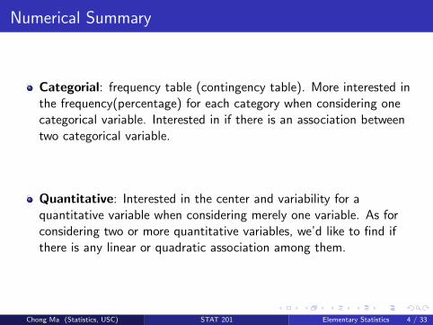
Categorial: frequency table (contingency table). More interested inthe frequency(percentage) for each category when considering onecategorical variable. Interested in if there is an association betweentwo categorical variable.
Quantitative: Interested in the center and variability for aquantitative variable when considering merely one variable. As forconsidering two or more quantitative variables, we’d like to find ifthere is any linear or quadratic association among them.
Chong Ma (Statistics, USC) STAT 201 Elementary Statistics 4 / 33

Example Alligator
What do alligators eat? For 219 alligators captured in four Florida lakes,researchers classified the primary food choice (in volume) found in thealligator’s stomach in one of the categories-fish, invertebrate(snails,insects, crayfish), reptile(turtles, baby alligators), bird or other(amphibian,mammal, plants). Data is available in Pearson statcrunch website.
Tips for making frequency (contingency) table in Statcrunch
stat → tables → frequency
stat → tables → contingency
Tips for making Pie Chart(Bar Plot) in Statcrunch
graph → Pie Chart → with data
graph → Bar Plot → with data
Chong Ma (Statistics, USC) STAT 201 Elementary Statistics 5 / 33

Pie Chart
Figure 1: Distribution of food for 219 alligators live in four lakes in Florida, whichare George, Hancock, Oklawaha and Trafford, respectively. About 43% ofalligators in the sample take fish as the primary food choice.
Chong Ma (Statistics, USC) STAT 201 Elementary Statistics 6 / 33

Bar plot
Figure 2: Bar plot for distribution of food for the 219 captured alligators.
Chong Ma (Statistics, USC) STAT 201 Elementary Statistics 7 / 33
Side-By-Side Pie Chart
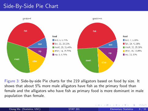
Figure 3: Side-by-side Pie charts for the 219 alligators based on food by size. Itshows that about 5% more male alligators have fish as the primary food thanfemale and the alligators who have fish as primary food is more dominant in malepopulation than female.
Chong Ma (Statistics, USC) STAT 201 Elementary Statistics 8 / 33

Frequency(Contingency) Table
Figure 4: 28.8% of the 219 capturedalligators in Florida live in George lake.
Figure 5: It indicates that there are moresmaller alligators in George and Hancocklakes and the opposite to Oklawaha andTrafford lake.
Chong Ma (Statistics, USC) STAT 201 Elementary Statistics 9 / 33
Example Cereal
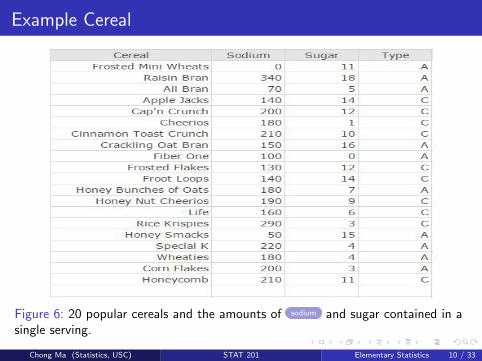
Figure 6: 20 popular cereals and the amounts of sodium and sugar contained in asingle serving.
Chong Ma (Statistics, USC) STAT 201 Elementary Statistics 10 / 33

Dot Plot
Tips for making Dot Plot in Statcrunch
graph → Dot Plot → select the variable of interest
Figure 7: Distribution of sodium in a single serving for 20 popular cereals. Most ofthe 20 cereals has amount of sodium between 50 and 230 mg in a single serving.
Chong Ma (Statistics, USC) STAT 201 Elementary Statistics 11 / 33

Stem-and-Leaf Plot
Tips for making Dot Plot in Statcrunch
graph → Stem and Leaf → select the variable of interest
Figure 8: The stem-and-leaf plot provides more information by stacking closevalues together for us to understand the distribution of the variable(sodium).However, both stem-and-leaf and dot plot are appropriate for a small data.
Chong Ma (Statistics, USC) STAT 201 Elementary Statistics 12 / 33

Histogram
Histogram
A histogram is a graph that uses bars to portray the frequencies or therelative frequencies of the possible outcomes for a quantitative variable.
The shape of a histogram(distribution)
modal: unimodal, bimodal or multi-modal
skewness: symmetric, left-skewed or right-skewed
How to decide the skewness
left-skewed: the left tail is longer than the right tail, e.g. life span
right-skewed: the right tail is longer than the left tail, e.g. income
Chong Ma (Statistics, USC) STAT 201 Elementary Statistics 13 / 33

Example STAT 201 Survey
Tips for making Histograms in Statcrunch
graph → Histogram → select the variable of interest
Figure 9: Distribution of STAT 201 students’ GPA. It shows us that the histogramis unimodal and left skewed.
Chong Ma (Statistics, USC) STAT 201 Elementary Statistics 14 / 33
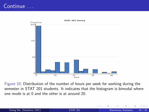
Continue . . .
Figure 10: Distribution of the number of hours per week for working during thesemester in STAT 201 students. It indicates that the histogram is bimodal whereone mode is at 0 and the other is at around 20.
Chong Ma (Statistics, USC) STAT 201 Elementary Statistics 15 / 33

Time Series Plot
Figure 11: Time series plot of month-average temperature in January, April, July,October and annual average temperature in New York Central Park in 1869-2012.
Chong Ma (Statistics, USC) STAT 201 Elementary Statistics 16 / 33

Center and Variability
Center: The mean and median
mean: x̄ = x1+...+xnn
median: x̃ is the middle value of the observations when observationsare ordered from the smallest to the largest. e.g.,
x1, x2, . . . , xn−1, xnordered→ x(1), x(2), . . . , x(n−1), x(n)
Variability: range, interquantile(IQR), and standard deviation(s)
range: difference between the largest and the smallest, i.e. x(n) − x(1)
IQR: the distance between the third and first quartiles, i.e. Q3 − Q1
s: the square root of the variance s2, which is an average of thesquares of the deviations from their mean, i.e.
s2 =
∑ni=1(xi − x̄)2
n − 1
Chong Ma (Statistics, USC) STAT 201 Elementary Statistics 17 / 33

Mean Vs. Median
Figure 12: Relationship between the mean and median. The median is usuallypreferred over the mean if the distribution is highly skewed because it betterdescribes what is typical; conversely, the mean is usually preferred. It is a goodidea to report both of the mean and median when describing the center of adistribution.
Chong Ma (Statistics, USC) STAT 201 Elementary Statistics 18 / 33

Continue . . .
Resistant
A numerical summary of the observations is called resistant if extremeobservations have little, if any, influence on its value.
Outlier
An outlier is an observation that falls well above or well below the overallbulk of the data.
Remark: The median is more resistant than the mean, because themedian is solely determined by having an equal number of observationsabove it and below it.
Chong Ma (Statistics, USC) STAT 201 Elementary Statistics 19 / 33

Example Cereal continue
In the example cereal in slide 10, the sodium in a single serving for 20brands are
0, 340, 70, 140, 200, 180, 210, 150, 100, 130
140, 180, 190, 160, 290, 50, 220, 180, 200, 210
Calculate the mean and median for the variable of sodium.
mean: x̄ = 0+340+···+200+21020 = 167
median: x̃ = 180Sort the values of sodium ascending
0, 50, 70, 100, 130, 140, 140, 150, 160, 180
180, 180, 190, 200, 200, 210, 210, 220, 290, 340
Chong Ma (Statistics, USC) STAT 201 Elementary Statistics 20 / 33
CO2 emissions 1
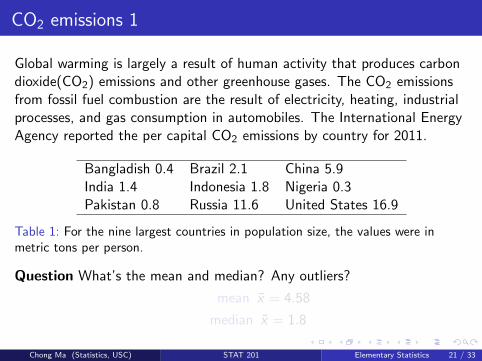
Global warming is largely a result of human activity that produces carbondioxide(CO2) emissions and other greenhouse gases. The CO2 emissionsfrom fossil fuel combustion are the result of electricity, heating, industrialprocesses, and gas consumption in automobiles. The International EnergyAgency reported the per capital CO2 emissions by country for 2011.
Bangladish 0.4 Brazil 2.1 China 5.9India 1.4 Indonesia 1.8 Nigeria 0.3Pakistan 0.8 Russia 11.6 United States 16.9
Table 1: For the nine largest countries in population size, the values were inmetric tons per person.
Question What’s the mean and median? Any outliers?
mean x̄ = 4.58
median x̃ = 1.8
Chong Ma (Statistics, USC) STAT 201 Elementary Statistics 21 / 33

CO2 emissions 1
Global warming is largely a result of human activity that produces carbondioxide(CO2) emissions and other greenhouse gases. The CO2 emissionsfrom fossil fuel combustion are the result of electricity, heating, industrialprocesses, and gas consumption in automobiles. The International EnergyAgency reported the per capital CO2 emissions by country for 2011.
Bangladish 0.4 Brazil 2.1 China 5.9India 1.4 Indonesia 1.8 Nigeria 0.3Pakistan 0.8 Russia 11.6 United States 16.9
Table 1: For the nine largest countries in population size, the values were inmetric tons per person.
Question What’s the mean and median? Any outliers?
mean x̄ = 4.58
median x̃ = 1.8
Chong Ma (Statistics, USC) STAT 201 Elementary Statistics 21 / 33

CO2 emissions 2
The International Energy Agency also reported the CO2 emissions(measured in gigatons,Gt) from fossil fuel combustion for the top 9countries in 2011.
Canada 0.5 China 8 India 1.8Iran 0.4 Germany 0.8 Japan 1.2Korea 0.6 Russia 1.7 United States 5.3
Table 2: CO2 emissions for the top 10 countries in 2011 and the values are in Gt.
Question What’s the mean and median? Any outliers?
mean x̄ = 2.26
median x̃ = 1.2
Chong Ma (Statistics, USC) STAT 201 Elementary Statistics 22 / 33

Variability-Standard Deviation
Name x x − x̄ (x − x̄)2
Canada 0.5 -1.76 3.08
China 8.0 5.74 32.99
India 1.8 0.46 0.21
Iran 0.4 -1.86 3.44
Germany 0.8 -1.46 2.12
Japan 1.2 -1.06 1.11
Korea 0.6 -1.66 2.74
Russia 1.7 -0.56 0.31
U.S. 5.3 -3.04 9.27
Total 20.3 0 55.28
Table 3: The mean is 2.26.The standard deviation s = 2.63.
s =
√∑9i=1(xi − x̄)2
n − 1=
√55.28
9− 1= 2.63
Chong Ma (Statistics, USC) STAT 201 Elementary Statistics 23 / 33

Five-number-summary
Definition (Percentile)
The pth percentile is a value such that p percent of the observations fallbelow or at that value.
The five-number-summary consists of minimum(x(1)), Q1, Q2(x̃), Q3, andmaximum(x(n)).
How to find quartiles:
Arrange the data in order.
Consider the median first, which is the second quartile Q2.
Consider the lower half of the observations (excluding the medianitself if n is odd). The median of these observations is the firstquartile Q1.
Consider the upper half of the observations (excluding the medianitself if n is odd). The median of these observations is the thirdquartile Q3.
Chong Ma (Statistics, USC) STAT 201 Elementary Statistics 24 / 33

Box Plot
Constructing a Box Plot
Draw a box going from Q1 to Q3.
Draw the median line inside the box.
Draw a line from the lower end of the box to the smallest observationthat is not a potential outlier. Draw a separate line from the upperend of the box to the largest observation that is not a potentialoutlier.
Draw the potential outliers with special symbols(e.g. a dot or a star).
Remark: An observation is called a potential outlier if it is more than1.5IQR below the first quartile(Q1) or above the thrid quartile(Q3)
Chong Ma (Statistics, USC) STAT 201 Elementary Statistics 25 / 33

CO2 Box Plot
The sorted CO2 emission in total for the top 9 countries are
0.4, 0.5, 0.6, 0.8, 1.2, 1.7, 1.8, 5.3, 8.0
The five-number-summary is
> summary(x2)
Min. 1st Qu. Median Mean 3rd Qu. Max.
0.400 0.600 1.200 2.256 1.800 8.000
Figure 13: The boxplot of the CO2 in total for the top 9 countries. It indicatesthere 2 countries are potential outliers.Chong Ma (Statistics, USC) STAT 201 Elementary Statistics 26 / 33
CO2 Box Plot
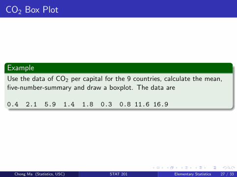
Example
Use the data of CO2 per capital for the 9 countries, calculate the mean,five-number-summary and draw a boxplot. The data are
0.4 2.1 5.9 1.4 1.8 0.3 0.8 11.6 16.9
Chong Ma (Statistics, USC) STAT 201 Elementary Statistics 27 / 33

Empirical Rule
Empirical Rule
If a distribution of data is bell shaped, the approximately
68% of the observations fall within 1 standard deviation of the mean,i.e., between the values of x̄ − s and x̄ + s(denoted x̄ ± s).
95% of the observations fall with 2 standard deviations of the mean(x̄ ± 2s).
All or nearly all observations fall within 3 standard deviations of themean(x̄ ± 3s).
Remark: If an observation falls beyond 3 standard deviations of themean, we say it a potental outlier.
Chong Ma (Statistics, USC) STAT 201 Elementary Statistics 28 / 33
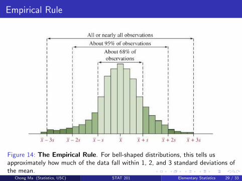
Empirical Rule
Figure 14: The Empirical Rule. For bell-shaped distributions, this tells usapproximately how much of the data fall within 1, 2, and 3 standard deviations ofthe mean.
Chong Ma (Statistics, USC) STAT 201 Elementary Statistics 29 / 33
Z-Score
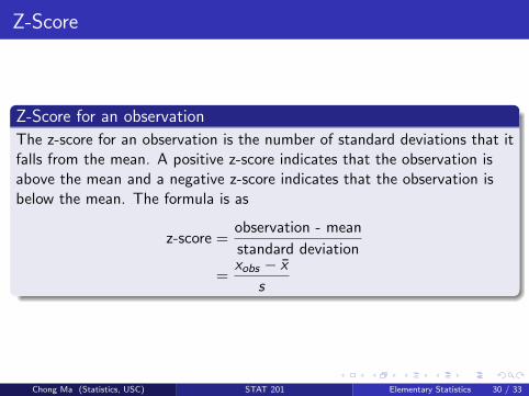
Z-Score for an observation
The z-score for an observation is the number of standard deviations that itfalls from the mean. A positive z-score indicates that the observation isabove the mean and a negative z-score indicates that the observation isbelow the mean. The formula is as
z-score =observation - mean
standard deviation
=xobs − x̄
s
Chong Ma (Statistics, USC) STAT 201 Elementary Statistics 30 / 33

Detecting Potential Outliers
1.5∗IQR: more than 1.5IQR below the first quartile(Q1) or above thethrid quartile(Q3).
Empirical Rule: z-score to fall more than 3 standard deviations fromthe mean where
z-score =observation −mean
standarddeviation
i.e., |Z-score > 3| ⇔ potential outlier
Chong Ma (Statistics, USC) STAT 201 Elementary Statistics 31 / 33

Exercise 1
College Students Heights For the 262 female and 117 male collegestudent heights, the average height for female is 65.4 inches and thestandard deviation is 3.3 inches; the average height for male is 70.9 inchesand the standard deviation 2.9 inches. The tallest female in this sample is91 inches and the shortest male in this sample is 62 inches.
1 Calculate the z-scores for the hight of 91 inches in the female groupand the hight of 62 in the male group.
2 Are they potential outliers in their corresponding group?
Chong Ma (Statistics, USC) STAT 201 Elementary Statistics 32 / 33

Exercise 2
Male heights According to a recent report from the U.S. National Centerfor Health Statistics, for males ages 25-34 years, 2% of their heights are 64inches or less, 27% are 68 inches or less, 54% are 70 inches or less, 80%are 72 inches or less, 93% are 74 inches or less and 98% are 76 inches orless. These are called cumulative percentages.
1 Which category has the median height?
2 Nearly all the heights fall between 60 and 80 inches, with fewer than1% falling outside that range. If the heights are approximatelybell-shaped, give a rough approximation for the standard deviation ofthe heights.
Chong Ma (Statistics, USC) STAT 201 Elementary Statistics 33 / 33


![[Notes]STAT1 - Elementary Statistics](https://img.dokumen.tips/doc/110x75/577cdbee1a28ab9e78a976c0/notesstat1-elementary-statistics.jpg)