16th International LS-DYNA® Users Conference Electromagnetics

June 10-11, 2020 1

Electrostatics and EM-ICFD Coupling in LS-DYNA®,

a Glimpse of Things to Come

Iñaki Çaldichoury1 Pierre L’Eplattenier1 1Livermore Software Technology, an Ansys company, Livermore, CA, USA

Abstract The EM LS-DYNA solver’s primarily focus is on Electromagnetic metal forming, Inducting heating, Resistive heating. Recently, its capabilities have been extended in the domains of battery charge/discharges, electrophysiology and spot welding. However, there is a domain of applications that gets periodically inquired about and users sometimes wonder whether LS-DYNA possesses any capabilities in that area. This area would be electrostatics. As it happens, the existing resistive heating solver can be used for certain applications by proceeding with an analogy between the Poisson equation for electrostatics and the Poisson equation for resistive heating, itself a derivative of Ohm’s law. Still, electrostatics often involves the calculation of the Coulomb force which is a surface force typically acting on the parts of a capacitor and for which no option was available for the user to do a coupled EM-structure analysis. From this, the idea sprung to solve the EM fields on the same mesh as the one provided by the ICFD solver. Indeed, the ICFD solver specializes in fluid structure interaction problems and has got extensive capabilities in transferring forces from the fluid surface to the solid as well as advanced dynamic mesh movement tracking and adaptive remeshing. In this paper, the current capabilities allowing the merging of the EM and ICFD solvers will therefore be described. Going beyond the domain of electrostatics, further applications which combine the domains of electromagnetic and fluids such as Magnetic Hydrodynamics (MHD) and Magnetorheological fluid (MRF) will be discussed.

The EM Solver for Electrostatics

The Resistive heating solver is commonly used to study the heat generated by a current flowing through a conductor and to see its effects on temperature. Recently, its capabilities have been extended for resistance Spot Welding applications, battery modelling and Electrophysiology. However, the same solver can also be used for some simple electrostatic applications. Indeed, one of the cornerstones of electrostatics amounts to finding the electric field 𝐸𝐸�⃗ for a given charge distribution 𝜌𝜌𝑓𝑓 therefore solving the following equation: ∇𝐷𝐷��⃗ = 𝜌𝜌𝑓𝑓 (1)

with 𝐷𝐷���⃗ , the electric displacement field, 𝐷𝐷��⃗ = 𝜀𝜀𝐸𝐸�⃗ where 𝜀𝜀 is the permittivity of the medium (𝜀𝜀 = 𝜀𝜀𝑟𝑟𝜀𝜀0, with 𝜀𝜀0, vacuum permittivity (perfect dielectric) and 𝜀𝜀𝑟𝑟 relative permittivity). Since the curl of the electric field is zero in static problems and consequently 𝐸𝐸���⃗ = −∇��⃗ 𝜑𝜑, the Poisson’s equation for electrostatics is produced: ∇. (𝜀𝜀𝑟𝑟∇��⃗ 𝜑𝜑) =

𝜌𝜌𝑓𝑓𝜀𝜀0

(2)

16th International LS-DYNA® Users Conference Electromagnetics

June 10-11, 2020 2

This equation is very similar to the equation solved by the resistive heating solver, with the relative permittivity of the medium playing the role of the conductivity. If the charge distribution is zero, then the Laplace equation is recovered. If required, the keyword *EM_EXTERNAL_FIELD can be used in order to add a density of charge (𝜌𝜌𝑓𝑓 ) to the r.h.s of the scalar potential equation: *EM_EXTERNAL FIELD FID FTYPE FDEF LCID

With FID the external field ID, FTYPE=3 for a charge density field type, FDEF=1 or 2 to define the field using a *DEFINE_CURVE ID or a *DEFINE_FUNCTION ID and LCID the identifier for the load curve or the define function. A quick verification of the solver’s behavior against the analytical solution for the capacity of a cylindrical capacitor is undertaken. The capacitance of a cylindrical geometry, admits an analytical solution given per unit length based on the outer and the inner radius: C = 2π𝜀𝜀𝑟𝑟𝜀𝜀0/ln (

𝑟𝑟0𝑟𝑟𝑖𝑖

) (3)

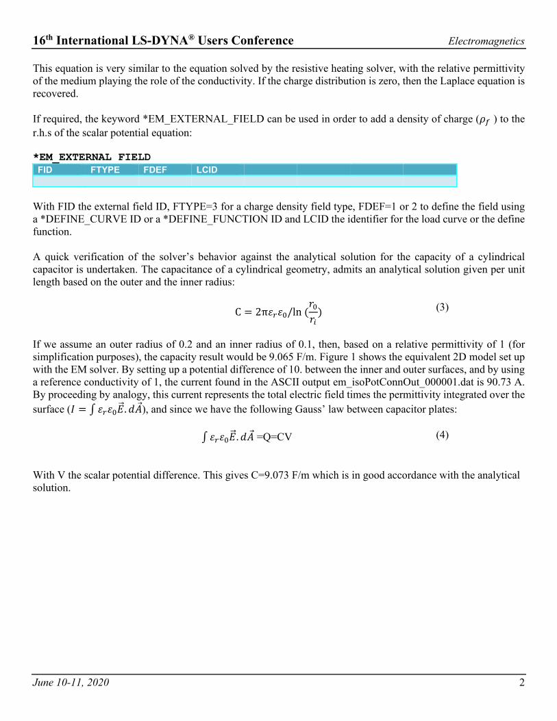
If we assume an outer radius of 0.2 and an inner radius of 0.1, then, based on a relative permittivity of 1 (for simplification purposes), the capacity result would be 9.065 F/m. Figure 1 shows the equivalent 2D model set up with the EM solver. By setting up a potential difference of 10. between the inner and outer surfaces, and by using a reference conductivity of 1, the current found in the ASCII output em_isoPotConnOut_000001.dat is 90.73 A. By proceeding by analogy, this current represents the total electric field times the permittivity integrated over the surface (𝐼𝐼 = ∫ 𝜀𝜀𝑟𝑟𝜀𝜀0𝐸𝐸�⃗ .𝑑𝑑𝐴𝐴), and since we have the following Gauss’ law between capacitor plates: ∫ 𝜀𝜀𝑟𝑟𝜀𝜀0𝐸𝐸�⃗ .𝑑𝑑𝐴𝐴 =Q=CV (4)

With V the scalar potential difference. This gives C=9.073 F/m which is in good accordance with the analytical solution.

16th International LS-DYNA® Users Conference Electromagnetics

June 10-11, 2020 3

Figure 1 2D cylindrical capacitor test

Coupling with the ICFD solver for Electrostatics applications On a conductor, a surface charge will experience a force in the presence of an electric field. This force is the average of the discontinuous electric field at the surface charge. This average in terms of the field just outside the surface amounts to the following electrostatic magneto pressure: 𝑃𝑃𝑚𝑚𝑚𝑚𝑚𝑚 =

𝜀𝜀02𝐸𝐸2 (5)

This pressure tends to draw the conductor into the field, regardless of the sign of the surface charge. From a numerical simulation perspective that surface force could be transferred to the solid for an electrostatic coupling between the structure and the surrounding dielectric volume. Since the ICFD solver already offers a similar coupling type for FSI applications at the interface between fluid mesh and structure mesh, it was decided to implement the capability of having the EM solver use the ICFD mesh structure and to be able to associate the fluid material to an EM material by defining a material type 3 : *EM_MAT_001/004

MID MTYPE SIGMA EOS

111 3

*ICFD_MAT

MID FLG RHO MU

111

16th International LS-DYNA® Users Conference Electromagnetics

June 10-11, 2020 4

Similarly, boundary conditions such as isopotentials defined by *EM_ISPOTENTIAL can be applied to fluid surface parts, i.e. *ICFD_PARTs: *EM_ISOPOTENTIAL

ISOID SETTYPE SETID

1 3 200

*ICFD_PART

PID SID MID

200

111

This allows to solve electrostatic cases such as the one described in the first part using an ICFD problem set up. Furthermore, the classic fluid pressure transferred in FSI applications can be replaced by the electrostatic magneto pressure by using the keyword *EM_CONTROL_COUPLING: *EM_CONTROL_COUPLING

THCPL SMCPL THLCID SMLCID FTHCPL FSMCPL

1

With FSMCPL, the coupling between fluid and the structure for the conductor parts. FSMCPL=0 means that the classic fluid pressure will be transferred to the structure, FSMCPL=1 means that the fluid pressure is replaced by the electrostatic magneto pressure given by Equation 5. FSMCPL=2 means that the two terms will be summed. Finally, since, for such applications, the actual solve of the fluid quantities are of no interest, it is recommended to use *ICFD_CONTROL_FSI=2 and *ICFD_BOUNDARY_GROUND for the wall parts so that the fluid values of velocity and pressure remain at zero at all times. Figure 1 shows an example of two capacitor plates where a potential difference has been applied between them. Progressively, the electrostatic force will bend those two plates and bring the edges closer together. Note that the ICFD solver automatically takes into account the EM scalar potential when using an adaptive mesh which can be controlled in *ICFD_CONTROL_ADAPT.

Figure 2 Electrostatic problem - Scalar Potential applied between two parallel capacitor plates. Coupling with the structure causes edges to deform.

Mesh Adaptivity is turned on.

16th International LS-DYNA® Users Conference Electromagnetics

June 10-11, 2020 5

Advanced EM/ICFD coupling application examples

Now that the capability of using the EM solver on an ICFD mesh has been introduced, many different applications involving multiple couplings are made possible. Figure 3 shows the three equations that can now be simultaneously solved in the fluid mesh. An application example for those capabilities would be the study of water inflow on a circuit board or another set of conductors and to study the consequences of the subsequent circuit shorts that are created. Figure 4 shows an example of such a configuration. In this example, at t=0 a column of water is being released on some battery tabs. The tabs have been defined as flexible so that the full nonlinear FSI problem is solved. The tabs are electrical conductors and connected to battery cells (not represented here) using the meshless model (See *EM_RANDLES_MESHLESS). The water has also been defined as electrically conductive so that, upon impact, a current path may be formed between the tabs which can will lead to an external short. The decay of the state of charge can be analyzed as well as the current generated. Figure 5 offers some examples of the post treatments available.

Figure 3 Equation system simultaneously solved when the fluid is defined as a conductor.

Figure 4 Water column impacting flexible battery tabs. A path is created for the current to flow between tabs generating an electric short and the

subsequent battery discharge. The curve shows the decrease of the State Of Charge of the battery due to the external short.

16th International LS-DYNA® Users Conference Electromagnetics

June 10-11, 2020 6

Figure 5 EM/ICFD/Solid mechanics post treatments examples

Conclusion and future developments The resolution of certain electrostatic problems has always been feasible by using the resistive heating solver and by proceeding by analogy. However, the addition of the option to define ICFD parts as conductors has allowed the solving of coupled applications with the possibility of transferring the electrostatic force to the structure. This has in turn further opened the door to a wide range of applications involving the coupling of the different electromagnetic and fluid mechanics physics, chief among them the study of water ingress on circuit components. Currently, this feature is only available with the EM resistive heating solver. However, in the future and based on user request, this may be extended to the Eddy current solver so that the effect of a magnetic field on a fluid flow may be studied. Species transport models are also under investigation for the CFD solver which would further extend the range of possibilities and Multiphysics couplings.