S1

ESI

Electronic Supplementary Information

Synthesis and reactivity of a trigonal porous nanographene on a gold surface

Rafal Zuzak,a Iago Pozo,b Mads Engelund,c Aran Garcia-Lekue,d Manuel Vilas-Varela,b José M. Alonso,b

Marek Szymonski,a Enrique Guitián,b Dolores Pérez,b Szymon Godlewski,a* Diego Peñab*

[a] Centre for Nanometer-Scale Science and Advanced Materials, NANOSAM, Faculty of Physics,

Astronomy and Applied Computer Science,

Jagiellonian University, Łojasiewicza 11, PL 30-348 Kraków, Poland.

[b] Centro de Investigación en Química Biolóxica e Materiais Moleculares (CiQUS) and

Departamento de Química Orgánica,

Universidade de Santiago de Compostela, 15782-Santiago de Compostela, Spain.

[c] Espeem S.A.R.L., L-4365 Esch-sur-Alzette,Luxembourg.

[d] Donostia International Physics Center, DIPC, Paseo Manuel de Lardizabal 4, E-20018 Donostia-

San Sebastian, Spain & IKERBASQUE, Basque Foundation for Science, E-48013 Bilbao, Spain.

SUPPORTING INFORMATION

Table of Contents Page

1. Experimental details and spectroscopic data S2

2. Additional nc-AFM images S7

3. Additional scanning tunneling spectroscopy (STS) data S8

4. STM images after 415 °C annealing S9

5. Calculation details S10

6. Structure of compound 8 S12

7. References S13

Electronic Supplementary Material (ESI) for Chemical Science.This journal is © The Royal Society of Chemistry 2019

S2

1. Experimental details and spectroscopic data

1.1. General methods

All reactions were carried out under argon using oven-dried glassware. THF, CH2Cl2, CH3CN and

DMF were purified by a MBraun SPS-800 Solvent Purification System. Finely powdered CsF was

dried under vacuum at 100 °C, cooled under argon and stored in a glove-box. Pd(PPh3)4 was

prepared from PdCl2 following a published procedure.1 Other commercial reagents were

purchased from ABCR GmbH, Sigma-Aldrich, Panreac or Fisher and were used without further

purification. TLC was performed on Merck silica gel 60 F254 and chromatograms were visualized

with UV light (254 and 360 nm). Column chromatography was performed on Merck silica gel 60

(ASTM 230-400 mesh). 1H and 13C NMR spectra were recorded at 300 and 75 MHz (Varian

Mercury-300 instrument) or 500 and 125 MHz (Varian Inova 500) respectively. MALDI-TOF

spectra were determined on a Bruker Autoflex instrument. Melting points were measured by a

Büchi melting point B-450 instrument. UV-Vis spectra were measured by a Jasco V-630

spectrometer. Fluorescence in solution was measured in a Fluoromax-2 spectrofluorimeter.

Triflate 3 was obtained in one step from commercially available starting materials, following a

published procedure (Scheme S1).2

Scheme S1. Synthesis of triflate 3.

S3

1.2. Synthesis of nanographene 2

Scheme S2. Synthesis of nanographene 2.

Over a solution of the polycyclic aryne precursor 3 (95 mg, 1 equiv) and Pd(PPh3)4 (16.5 mg, 0.1

equiv) in CH3CN/THF (5:1, 12 mL), CsF (65 mg, 4 equiv.) was added. The mixture was heated at

60 °C and stirred for 16h. Then, the reaction crude was filtered and washed with CH3CN

(2x10mL) and Et2O (2x10mL). The resulting solid was extracted in a Soxhlet apparatus with

CHCl3 overnight. The solvent was removed under reduced pressure obtaining product 2 (23

mg, 37 % yield) as a white solid (m.p.: >400 ˚C).

1H NMR (500 MHz, C2D2Cl4), δ: 8.42 (s, 6H); 7.21-7.02 (m, 30H); 6.89-6.71 (m, 30H) ppm.

13C NMR-DEPT (125 MHz, C2D2Cl4), δ: 131.4 (C), 131.2 (CH), 131.0 (CH), 129.0 (C), 127.4 (CH)

126.9 (CH) 126.4 (CH), 125.1 (CH), 122.1 (CH) ppm.

MS (APCI), m/z: 1291.52 (M++1).

HRMS (APCI), m/z: found 1291.5235 (calc. for C102H67, calcd: 1291.5237).

S4

1.3. Synthesis of nanographene 5

Scheme S3. Synthesis of nanographene 5.

Over a suspension of compound 2 (13 mg, 1 equiv) in CH2Cl2 (20mL) at 0 °C, DDQ (23 mg, 10

equiv) was added. After 5 min, TfOH (1 mL) was added and the reaction mixture was stirred at

0 °C for 30 min. Then, 20 mL of NaHCO3 (saturated aqueous solution) were added. The mixture

was extracted with CH2Cl2 (3x20 mL) and hot C2H2Cl4 (5 mL). The volatiles were removed under

reduced pressure. The obtained residue was washed with H2O (2x10 mL), MeOH (2x10 mL) and

Et2O (2x10 mL) obtaining product 5 as a dark solid (3.1 mg). The extreme insolubility of

compound 5 precluded its NMR characterization.

MALDI-TOF: 1273.2.

S5

1.4. 1H and 13C NMR spectra of compound 2.

Figure S1. NMR spectra of compound 2 in C2D2Cl4.

ppm (t1)

0.01.02.03.04.05.06.07.08.09.010.0

ppm (f1)

121.0122.0123.0124.0125.0126.0127.0128.0129.0130.0131.0132.0133.0134.0

ppm (f1)

121.0122.0123.0124.0125.0126.0127.0128.0129.0130.0131.0132.0133.0134.0

S6

1.5. UV/Vis and emission spectra of compound 2.

Figure S2. Absorption spectra of compound 2 in CH2Cl2.

Figure S3. Emission spectra of compound 2 in CH2Cl2.

.

S7

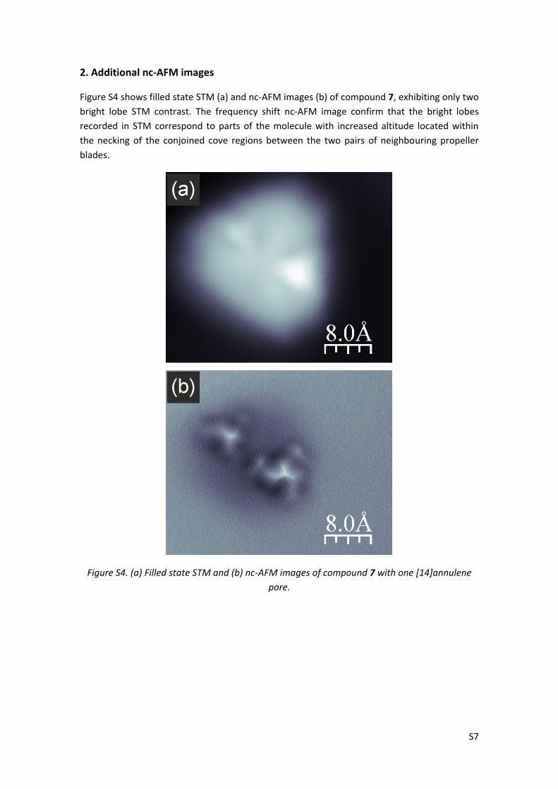
2. Additional nc-AFM images

Figure S4 shows filled state STM (a) and nc-AFM images (b) of compound 7, exhibiting only two

bright lobe STM contrast. The frequency shift nc-AFM image confirm that the bright lobes

recorded in STM correspond to parts of the molecule with increased altitude located within

the necking of the conjoined cove regions between the two pairs of neighbouring propeller

blades.

Figure S4. (a) Filled state STM and (b) nc-AFM images of compound 7 with one [14]annulene

pore.

S8

3. Additional scanning tunneling spectroscopy (STS) data

Figure S5 shows single point scanning tunnelling spectroscopy curves acquired for compound

1, that is, a molecule with three [14]annulene rings embedded, after cyclodehydrogenation

induced at 370 °C. Middle panel shows constant current dI/dV maps recorded for voltages at

which single point STS resonances in panels (a, filled states) and (b, empty states) are

captured. Comparison between experimental maps and simulated ones is shown for HOMO-2,

HOMO-1, HOMO, LUMO, LUMO+1 and LUMO+2 states in Figure 5 of the main text.

Interestingly within the filled state part of the STS spectra pronounced resonances in the range

of a Au(111) surface state appear. However the spatial dI/dV maps recorded for these voltages

do not show any intramolecular contrast over the molecule and we interpret the presence of

above described resonances as a manifest of the Au(111) surface state.

Figure S5. Scanning tunnelling spectroscopy (STS) data recorded for compound 1 with three

[14]annulene rings incorporated; (a) and (c) filled- and empty-state single point STS curves

recorded for different planar tip positions indicated by coloured crosses within the insets, (b)

spatial dI/dV maps recorded for voltages indicated in (a,c) by vertical dashed violet lines.

S9

4. STM images after 415 °C annealing

Figure S6 shows additional STM images of the molecules after annealing at 415 °C. Figure S6a

indicates that the molecules tend to locate within the elbows of the surface herringbone

pattern. Additional high resolution images acquired with the tip functionalized with a CO

molecule are shown in Figures S6b,c. In each case the molecular topography contains one

darker shadow with a faint lobe in the middle, as well as additional subtle shadows which vary

slightly from molecule to molecule. This might indicate on differences in the molecule

transformations upon annealing at 415 °C.

Figure S6. Additional filled state STM images of molecules after 415 °C annealing, (a) overview

image indicating on the location of molecules within the elbows of a surface herringbone

pattern; (b) and (c) high resolution filled state STM images acquired with the tip functionalized

by a CO molecule showing subtle differences between individual molecules, scanning

parameters: tunnelling current 50 pA (a,b), 100 pA (c), bias voltage -1.0V

S10

5. Calculation details

Due to the large size of the molecule a full simulation including the Au substrate prove

infeasible due to computational cost. In our case, however, the molecule-only model is

reasonable, due to the anticipated weak substrate interaction as well as the substantial

internal strain in the molecule. However, to retain the alignment effect of a surface we

applied a weak asymmetric model potential 𝑃(𝑟) =𝑎

𝑟2−

𝑏

𝑟 (a=0.2 eV·Å 2, b=0.2 eV·Å).

Geometric relaxations were performed via density-functional theory using the SIESTA

code.3,Our model: We used a double-zeta-polarized(DZP) basis set with orbital radii defined

using a 100 meV energy shift, the Perdew–Burke–Ernzerhof(PBE) version of the generalized

gradient approximation for exchange–correlation,4 a real-space grid equivalent to a 200 Ry

plane-wave cutoff. Forces were relaxed until forces were smaller than 0.02 eV/Å.

To compute the STM images we followed the surface integration technique of Paz and Soler. 5

In addition, we used the Tersoff–Hamann approximation 6 assuming a proportionality factor of

1 nA·Å-3 for the ratio between the local density of states. dI/dV maps were simulated by first

calculating current and differential current independently on a 3D grid and then interpolating

the differential current to the current isosurface corresponding to the target current.

In order to mimic the effect of spatial uncertainty in the measurement which reduces the

resolution of the STM images, we have convoluted our currents with a Gaussian kernel

𝐾(𝑟, 𝑟0) = (𝜋 ∙ 𝜎2)3/2 ∙ 𝑒𝑥𝑝 (|𝑟−𝑟0|

2

2𝑠2). To emulate the experimental process of taking dI/dV

maps the tip height was determined using a target current of 1 nA with a, by design, large

spatial uncertainty (sigma=2.0 Å), while the differential current was subsequently calculated at

a low spatial uncertainty (sigma=0.5 Å). Based on experimental peak widths we used a spectral

broadening of 0.2 V.

Molecular orbitals were, as well, generated with the Paz/Soler technique. The isosurface of the

absolute value of the orbital was first generated using the density isovalue corresponding to

the STM Tersoff-Hamann current isovalue. Then the opposite phases of the orbital were

plotted in blue/red while the colour intensity shows the relative spatial height of the orbital

(white->black, minimum->maximum) and plotted to give the maximal correspondence with

the STM simulations.

For clarity the single electron molecular orbitals are denoted with ‘, whereas molecular states

which may be composed of one or more molecular orbitals are denoted without ‘.

S11

Figure S7. Calculated molecular orbital wavefunctions for compound 1, upper panel shows

unoccupied molecular orbitals, lower panels presents filled orbitals, middle section indicates

the energies of individual molecular states. The middle of the HOMO-LUMO gap is chosen as

the zero of energy.

The geometry of the transformed porous nanographene (Fig. 6b) was optimized using density

functional theory as implemented in the SIESTA code.3 All the atoms were relaxed until forces

were < 0.01eV/Ang, and the dispersion interactions were taken into account by the non-local

optB88-vdW functional.7 The basis set consisted of double zeta plus polarization (DZP) orbitals

and diffuse 3s and 3p orbitals for C atoms, and DZP orbitals for Au and H atoms. A cutoff of 300

Ry was used for the real-space grid integrations and the Γ -point approximation for sampling

the three-dimensional Brillouin zone.

S12

6. Structure of compound 8

Figure S8. Compound 8 detected after subjecting nanographene 1 to thermal annealing at 415 oC.

S13

7. References

1. (a) L. S. Hegedus, Palladium in Organic Synthesis. In Organometallics in Synthesis: A Manual;

M. Schlosser, Ed.; John Wiley & Sons: New York, 1994; (b) M. M. Huq, M. R. Rahman, M. Naher,

M. M. R. Khan, M. K. Masud, G. M. G. Hossain, N. Zhu, Y. H. Lo, M. Younus, W. Wong, J. Inorg.

Organomet. Polym., 2016, 26, 1243-1252.

2. D. Rodríguez-Lojo, D. Peña, D. Pérez, E. Guitián, Synlett, 2015, 26, 1633-1637.

3. J. M. Soler, E. Artacho, J. D. Gale, A. Garcia, J. Junquera, P. Ordejón, and D. Sanchez-Portal, J.

Phys. Condens. Matter, 2002, 14, 2745-2779.

4. J. P. Perdew, K. Burke and M. Erzerhof, Phys. Rev. Lett., 1996, 77, 3865-3868.

5. O. Paz and J. M. Soler, Phys. Stat. Sol. (b), 2006, 243, 1080-1094.

6. J. Tersoff and D. R. Hamann, Phys. Rev. Lett., 1983, 50, 1998-2001.

7. J. Klimes, D. R. Bowler, and A. Michaelides, J. Phys. Condens. Matter, 2010, 22, 022201.