ELECTROMAGNETIC FIELD COUPLING TO … · Keywords: Buried wires, antenna model, transmission line approximation, set of pocklington integro-differential equations, numerical solution

D. Poljak et al., Int. J. Comp. Meth. and Exp. Meas., Vol. 1, No. 2 (2013) 142–163

© 2013 WIT Press, www.witpress.comISSN: 2046-0546 (paper format), ISSN: 2046-0554 (online), http://journals.witpress.comDOI: 10.2495/CMEM-V1-N2-142-163

ELECTROMAGNETIC FIELD COUPLING TO ARBITRARY WIRE CONFIGURATIONS BURIED IN A LOSSY GROUND: A REVIEW OF ANTENNA MODEL AND TRANSMISSION

LINE APPROACH

DRAGAN POLJAK1, KHALIL EL-KHAMLICHI DRISSI2 & BACHIR NEKHOUL3

1Department of Electronics, University of Split, Split, Croatia.2Pascal Institute, Blaise Pascal University, Clermont-Ferrand, France.

3LAMEL Laboratory, University of Jijel, Algeria.

ABSTRACTThe paper deals with two different approaches for the analysis of electromagnetic fi eld coupling to arbitrary wire confi gurations buried in a lossy medium: the wire antenna theory and the transmission line method. The wire antenna formulation deals with the corresponding set of Pocklington integro-differential equation, while the transmission line model is based on the telegrapher’s equations. The set of Pocklington equations is solved via the Galerkin–Bubnov scheme of the indirect boundary element method, while the telegrapher’s equations are treated using the chain matrix method and fi nite differ-ence technique, respectively. A number of illustrative computational examples pertaining to buried multiple lines and grounding systems is given in the paper.Keywords: Buried wires, antenna model, transmission line approximation, set of pocklington integro-differential equations, numerical solution methods.

1 INTRODUCTIONThe analysis of electromagnetic fi eld coupling to thin wire confi gurations buried in a lossy medium is important in many electromagnetic compatibility (EMC) applications, e.g. communications and power cables, geophysical investigations, grounding systems, etc. This problem can be analyzed in either frequency or time domain by using the transmission line (TL) model, or thin wire antenna theory (AT) (full-wave model) [1, 2] with the latter being considered as a more rigorous one. The TL approach is quite plausible approximation for long straight conductors with electrically small cross sections but it is not valid for fi nite length wires, wires of arbitrary shape and high frequency excitations. Consequently, AT has to be used.

On the other hand, a principal drawback of the wire AT applied to buried conductors is rather high computational cost. Using enhanced TL model it is possible to overcome some limitations of the model restrictions. Thus, a rigorous relationship between frequency domain TL equations and integral relationships arising from the wire AT for the single wire below ground has been reported in [3].

The comparison between frequency domain wire antenna model and TL model pertaining to a single buried conductor has been presented in [4] and, quite recently, in [5]. The analy-sis has been extended to multiple buried wires, as well [6]. The formulation used in [6] arises from the wire AT and is based on the set of the Pocklington integro-differential equa-tions for half-space problems. The TL model discussed in [4–6] is related to the telegrapher’s equations. The set of the Pocklington equations is numerically handled via the frequency domain Galerkin–Bubnov scheme of the indirect boundary element method (GB-IBEM) [2]. The telegrapher’s equations, arising from TL model, are treated using the chain matrix method [4–6].

D. Poljak et al., Int. J. Comp. Meth. and Exp. Meas., Vol. 1, No. 2 (2013) 143

Furthermore, a transient analysis of complex grounding systems using both AT and TL approximation has been presented in [7–9] for a single horizontal grounding electrode and complex grounding systems, respectively.

This paper reviews the analysis methods of electromagnetic coupling to buried wire con-fi gurations in the frequency domain [4–10].

The full wave approach and approximate TL approaches are discussed throughout the paper and a trade-off between these techniques has been stressed out. Modeling of multiple buried conductors and grounding systems are presented in separate sections.

A number of illustrative computational examples pertaining to buried conductors and grounding systems is given throughout the paper.

2 BURIED LINESThis section compares the wire AT approach to the TL approach in the modeling of electro-magnetic coupling to buried conductors in the frequency domain. The AT approach is based on the set of Pocklington integro-differential equations for arbitrary wires. The presence of a lossy half-space is taken into account by means of approximate refl ection coeffi cient (RC) approach [11]. The resulting integro-differential equations are numerically solved via a fre-quency domain version of the GB-IBEM. The TL model in the frequency domain is based on the corresponding telegrapher’s equations which are treated using the chain matrix method.

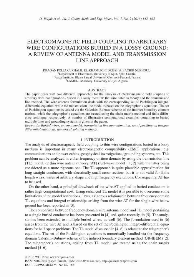
The geometry of interest is related to multiple horizontal conductors buried in a lossy ground, as shown in Fig. 1.

The present analysis deals with the frequency response of buried conductors confi gura-tions using the AT and TL approach, respectively.

2.1 Antenna theory approach: set of coupled Pocklington equations for arbitrary wire confi gurations

The set of Pocklington equations for multiple buried wires of arbitrary shape can be readily derived as an extension of the Pocklington integro-differential equation for a single buried

z

x

y

ε, m0, σ

ε0, m0ErHr

h 1

h 2 h 3

L

Figure 1: The geometry of horizontal buried lines.

144 D. Poljak et al., Int. J. Comp. Meth. and Exp. Meas., Vol. 1, No. 2 (2013)

wire enforcing the continuity condition for the tangential fi eld component along the thin wire surface [10].

The wire placed in an infi nite lossy medium is fi rst considered, and then the formulation is extended to a corresponding half space problem.

Assuming the perfectly conducting wire, the total fi eld composed from the excitation fi eld �excE and scattered fi eld

�sctE vanishes:

( ) 0exc scts E E⋅ + =� ��

on the wire surface (1)

where �s is the unit vector tangent at the observation point.

Starting from Maxwell’s equations and the Lorentz gauge, the scattered fi eld can be expressed in terms of the vector potential

�:A

1 ( )sct

efec

E j A Aj

wwme

= − + ∇ ∇� ��

(2)

The magnetic vector potential is defi ned by the particular integral:

0( ) ( ') ( , ') ' '

4 C

A s I s g s s s dsm

p= ∫

� � (3)

where I(s′) is the induced current along the line, �s' is the unit vector tangent at the source

point and g0(s,s′) is the corresponding Green’s function of the form:

1 0

00

( , ')jk Reg s s

R

−

= (4)

while R0 is the distances from the source to the observation point, respectively:

( ) ( ) ( )2 2 2 2

0 ' ' 'R x x y y z z a= − + − + − + (5)

where a denotes the wire radius.Combining eqns (1)–(5) leads to the Pocklington integro-differential equation for the

unknown current distribution along the single wire of an arbitrary shape insulated in an unbounded lossy medium [9, 10]:

( ) ( ) ( )2

1 0'

1 ' ' , ' '4

exc

eff C

E s I s s s k g s s dsj pwe

⎡ ⎤= − ⋅ ⋅ ⋅ + ∇∇⎣ ⎦∫ � � (6)

Integral equation for an infi nite lossy medium (6) can be extended to a case of a thin wire located near the interface between two media by modifying the kernel to account for the electric fi eld refl ecting from the interface.

The excitation fi eld component then can be written as the sum of the incident fi eld �

incE and the fi eld refl ected from the interface

�refE , i.e.

= +� � �

exc inc refE E E (7)


while the refl ected fi eld �

refE is given by

( )( ) ( )

( ) ( )

2 220 112 2

0 1 '

'

' * , * '1

4 ' * , ' '

irefC

effs

C

k kI s s k g s s ds

k kE sj I s s G s s dspwe

⎡ ⎤− ⎡ ⎤⋅ ⋅ + ∇∇ +⎢ ⎥⎣ ⎦+⎢ ⎥=⎢ ⎥+ ⋅ ⋅⎢ ⎥⎣ ⎦

∫

∫

��

� (8)

The Green’s function gi(s,s*) arising from the image theory is:

( )

1 1

1

, *jk R

ieg s s

R

−

= (9)

with R1 being the distance from the image point to the observation point, respectively, *�s is the unit vector tangential at the source point of the image wire, while k0 and k1 are propaga-tion constants of air and lossy ground, respectively:

2 20 0 0w m e=k (10)

2 21 0 effk w m e= (11)

The complex permittivity of the lossy ground εeff is given by

0eff r j s

e e ew

= − (12)

where er and s are relative permittivity and conductivity of the ground, respectively, and w is the operating frequency.

The kernel Gs(s,s′)

( ) ( ) ( ) ( ) ( ), ' ' 'H H H V V

s x z z z z zG s s e s G e G e G e e s G e G er r r r= ⋅ ⋅ ⋅ + ⋅ + ⋅ + ⋅ ⋅ ⋅ + ⋅��

f f (13)

is a correction term containing the Sommerfeld integrals and involves the following compo-nents for horizontal and vertical dipoles [11, 12]:

220r

r

∂=

∂ ∂V RG k V

z (14)

22 21 02

V RzG k k V

z⎛ ⎞∂

= +⎜ ⎟∂⎝ ⎠ (15)

22 21 12cosH R RG k V k Ur

r

⎛ ⎞∂= +⎜ ⎟∂⎝ ⎠

f (16)

2 21 1

1sinH R RG k V k Ur r

⎛ ⎞∂= − +⎜ ⎟⎝ ∂ ⎠f f (17)

4 cosH Vz efecG j Grpwe= − f (18)


The Sommerfeld integral terms are:

( ) ( )1 '

1 00

z zRU D e J dgl lr l l

∞− += ∫ (19)

( ) ( )1 '

2 00

z zRV D e J dgl lr l l

∞− += ∫ (20)

where

( ) ( )

21

1 2 20 1 1 1 0

2 2l

g g g= −

+ +kD

k k (21)

( ) ( )2 2 2 2 21 0 0 1 1 1 0

2 2Dk k k k

lg g g

= −+ +

(22)

and

2 2 2 2

0 0 1 1;k kg l g l= − = − (23)

Finally, combining eqns (1), (6), (7) and (8) yields the Pocklington integro-differential equa-tion for the unknown current distribution along the single wire antenna of arbitrary shape buried in a lossy ground

( )

( ) ( )

( ) ( )

( ) ( )

21 0

'

2 220 112 2

0 1 '

'

' ' , ' '

1 ' * , * '4

' * , ' '

C

excs i

eff C

sC

I s s s k g s s ds

k kE s I s s s k g s s ds

j k k

I s s s G s s ds

pwe

⎡ ⎤⎡ ⎤⋅ ⋅ ⋅ + ∇∇ +⎣ ⎦⎢ ⎥⎢ ⎥

−⎢ ⎥⎡ ⎤= − + ⋅ ⋅ ⋅ + ∇∇ +⎣ ⎦⎢ ⎥+⎢ ⎥⎢ ⎥+ ⋅ ⋅ ⋅⎢ ⎥⎣ ⎦

∫

∫

∫

� �

� �

� �

(24)

To derive the corresponding set of coupled Pocklington integro-differential equations for NW wires of arbitrary shape the infl uence of each antenna has to be summarized, i.e. it follows:

( )

( ) ( )

( ) ( )

( ) ( )

21 0

'

2 220 112 2

1 0 1 '

'

' ' , ' '

1 ' * , * '4

' * , ' '

1,2,...,

n

W

n

n

n n m n n m n nC

Nexcsm m n n m n inm m n n

neff C

n n m n s m n nC

W

I s s s k g s s ds

k kE s I s s s k g s s ds

j k k

I s s s G s s ds

m N

pwe =

⎡ ⎤⎡ ⎤⋅ ⋅ ⋅ + ∇∇ +⎣ ⎦⎢ ⎥⎢ ⎥⎢ ⎥− ⎡ ⎤= − + ⋅ ⋅ ⋅ + ∇∇ +⎢ ⎥⎣ ⎦+⎢ ⎥⎢ ⎥+ ⋅ ⋅ ⋅⎢ ⎥

⎢ ⎥⎣ ⎦=

∫

∑ ∫

∫

� �

� �

� �

(25)


An approximate simplifi ed form of Green’s function containing refl ection coeffi cient, deduced from the rigorous approach involving the Sommerfeld integrals, for overhead wires has been reported in [11]. Similarly, for the case of multiple buried wires the integral equation set (25) becomes [6]:

( )

( )

( )

( ) ( ) ( )

22 *1 0

0

22 *1

1

22 *1

, ''

1 , *4 *

, * ' '*

n

w

L

m n mn m nm n

Nexcsm m TM m n imn m n

neff m n

TE TM m m m n imn m n n nm n

k s s g s ss s

E s R k s s g s sj s s

R R s p k p s g s s I s dsp s

m

pwe =

⎡ ⎤⎧⎡ ⎤∂⎪ − +⎢ ⎥⎨⎢ ⎥∂ ∂⎪⎢ ⎥⎣ ⎦⎩⎢ ⎥

⎡ ⎤∂⎢ ⎥= − + − +⎢ ⎥⎢ ⎥∂ ∂⎣ ⎦⎢ ⎥⎢ ⎥⎫⎡ ⎤∂ ⎪⎢ ⎥+ − ⋅ ⋅ − ⎬⎢ ⎥∂ ∂⎢ ⎥⎪⎣ ⎦ ⎭⎣ ⎦

∫

∑

� �

� �

� � � �

1,2,..., WN=

(26)

where RTM and RTE are the refl ection coeffi cients for the case of transverse magnetic and transverse electric polarization, respectively, given by [6]:

2

2

1 1cos ' sin '

1 1cos ' sin 'TM

n nR

n n

q q

q q

− −=

+ − (27)

2

2

1cos ' sin '

1cos ' sin 'TE

nR

n

q q

q q

− −=

+ − (28)

where In(sn′) is the unknown current distribution along the n-th wire, ( )excmE s the excitation

function on the m-th wire, g0,nm(sm, sn′) the free space Green’s function, while gi,nm(sm, sn*)

arises from the image theory and 0

.effne

e=

The principal advantage of the RC approach versus rigorous Sommerfeld approach is sim-plicity of the formulation and appreciably less computational cost. Generally, RC approach produces results roughly within 10% of those obtained via rigorous Sommerfeld integral approach [11].

2.2 Antenna theory approach: numerical solution

The set of integral equations (26) is handled via an effi cient GB-IBEM. The essence of the method has been presented in detail in [2]. Some special features related to isoparametric elements implementation have been discussed recently in [10].

The unknown current ( )zenI along the n-th wire segment is expressed in terms of linearly

independent basis functions fni, with unknown complex coeffi cients Ini:


( ) { } { }

1

' ( ')n

Ten ni ni n n

i

I s I f s = f I=

= ∑ (29)

and the use of isoparametric elements yields:

( ) { } { }

1

( )n

Ten ni ni n n

i

I I f = f Iz z=

= ∑ (30)

where n is the number of local nodes per element.A linear approximation over a wire segment is used in this work and the corresponding

shape functions are given by:

1 2

1 12 2

f fz z− += = (31)

as this choice was proved to be optimal for numerical treatment of various wire structures [2]. Applying the weighted residual approach and implementing the Galekin–Bubnov proce-

dure the set of Pocklington equations is transformed into a system of algebraic equations. Performing some mathematical manipulations, the following matrix equation is obtained:

� �

� �

0

21 0

2 20 12 2

20 11

( ) ( ' )( , ' ) '

'

' ( ) ( ' ) ( , ' ) '

( ) ( ' )( , * ) '

*

* ( ) ( ' )

m n

m n

m n

jm m in nnm m n n m

m nl l

m n jm m in n nm m n n ml l

jm m in ninm m n n m

m nl l

m n jm m in n

df s df sg s s ds ds

ds ds

k s s f s f s g s s ds ds

df s df sg s s ds ds

ds dsk kk k k s s f s f s g

Δ Δ

Δ Δ

Δ Δ

−

+ ⋅ ⋅

− +−

++ + ⋅ ⋅

∫ ∫

∫ ∫

∫ ∫

� �

{ }ni1 1

( , * ) '

' ( ) ( ' ) ( , ' ) '

4 ( ) ( ) 0; 1,2,....., ; 1,2,.....,

m n

m n

m

Nw Nn

n i

inm m n n ml l

m n jm m in n snm m n n ml l

treff sm m jm m m W

l

I

s s ds ds

s s f s f s G s s ds ds

j E s f s ds m N j Npwe

= =

Δ Δ

Δ Δ

Δ

⎧ ⎫⎪ ⎪⎪ ⎪⎪ ⎪⎪ ⎪⎪ ⎪⎪ ⎪⎪ ⎪⎡ ⎤⎨ ⎬⎢ ⎥⎪ ⎪⎢ ⎥ +⎪ ⎪⎢ ⎥⎪ ⎪⎢ ⎥⎪ ⎪⎣ ⎦⎪ ⎪

+ ⋅⎪ ⎪⎪ ⎪⎩ ⎭

= − = =

∑∑

∫ ∫

∫ ∫

∫ m

(32)

where Nm is the number of elements on the m-th antenna and Nn is the number of elements on the n-th antenna.

Equation (32) can also be, for convenience, written in the matrix form:

[ ] { } { }i j

1 1

= , m =1,2,..., ; j =1,2,...,w nN N

en m w mji

n i

Z I V N N= =

∑∑ (33)

where [Zji] is the mutual impedance matrix for the j-th observation segment on the m-th wire and i-th source segment on the n-th antenna.


The use of isoparametric elements results in the following expression for mutual imped-ance matrix:

[ ] { } { }

� � { } { }

{ } { }

� � { } { }

1 1

01 1

1 121 0

1 1

1 1

2 21 10 1

2 20 1 2

1

' ( , ' ) ''

' ' ( , ' ) ''

' ( , * ) ''

* ' ( , * ) ''

e T n mnm m nji j i

T n mm n nm m nj i

T n minm m nj i

T nm n inm m nj i

ds dsZ D D g s s d d

d d

ds dsk s s f f g s s d d

d d

ds dsD D g s s d d

d dk kk k ds d

k s s f f g s s dd

z zz z

z zz z

z zz z

zz

− −

− −

− −

= −

+ ⋅ ⋅ +

− +−

++

+ ⋅ ⋅

∫ ∫

∫ ∫

∫ ∫

� � { } { }

1 1

1 1

1 1

1 1

' ' ( , ' ) ''

m

T n mm n snm m nj i

sd

d

ds dss s f f G s s d d

d d

zz

z zz z

− −

− −

⎡ ⎤⎢ ⎥⎢ ⎥ +⎢ ⎥⎢ ⎥⎢ ⎥⎣ ⎦

+ ⋅

∫ ∫

∫ ∫

(34)

Note that matrices {f} and {f ′} contain the shape functions while {D} and {D ′} contain their derivatives.

The voltage vector is given by:

{ }

1

1

4 ( ) ( ) , 1,2,....., ; 1,2,.....,m

m inc meff s m jm m m W mj

dsV j E s f s d m N j N

dpwe x

x−

= − = =∫ (35)

and can be evaluated in the close form [10].

2.3 Transmission line approximation

Voltages and currents along the multiple buried conductors shown in Fig. 1 induced by an external fi eld excitation can be determined from the fi eld-to-transmission line matrix equa-tions in the frequency domain [5]:

( ) ( ) ( )ˆ ˆ ˆ ˆ. F

d V x Z I x V xdx

⎡ ⎤ ⎡ ⎤ ⎡ ⎤ ⎡ ⎤+ =⎣ ⎦ ⎣ ⎦ ⎣ ⎦ ⎣ ⎦ (36)

( ) ( ) ( )ˆ ˆ ˆ ˆ. F

d I x Y V x I xdx

⎡ ⎤ ⎡ ⎤ ⎡ ⎤ ⎡ ⎤+ =⎣ ⎦ ⎣ ⎦ ⎣ ⎦ ⎣ ⎦ (37)

The procedures for the assessment of longitudinal impedance matrix [ ]∧Z and the transversal

admittance matrix ˆ[ ]Y are discussed in detail in [1]. The solution of the frequency domain TL equations is based on the chain matrix discussed in [3]. The per unit length parameters R, L, C and G of buried conductors are evaluated using the modal equation available in [13] and are frequency dependent. Such an approach is more accurate than use of well-known Pol-aczeck formulas [1]. The standard TL and modifi ed TL (MTL) [5] approach are both used, respectively.

It is worth emphasizing that the TL theory can handle the problem of electromagnetic coupling directly in time but without considering the impact of frequency on the parameters


per unit length (in the expression of Z impedance). The direct time domain solution of TL equations requires the numerical calculation of a convolution integral which is a rather tedi-ous task as the correction term includes the fi nite conductivity of the soil within the impedance Z. Moreover, this term is not available in the closed form and the inverse Fourier transform (IFT) algorithm has to be used.

2.4 Computational examples

Numerical results presented in this section are related to various confi gurations of three buried conductors.

The electric fi eld of the transmitted plane wave exciting multiple wires confi guration at certain burial depth z is [6]:

1

0jk ztr

TME E e−= Γ (38)

where E0 is the fi eld amplitude and the point of reference is located at the interface of two media z = 0. Note that E0 = 1 V/m in all examples to follow. Also, all numerical results obtained via GB-IBEM (abbreviated as BEM in fi gures to follow), standard TL and MTL, respectively are compared to the results calculated via NEC (numerical electromagnetic code) [14] with Sommerfeld approach and RC approximation, respectively. Figure 2 shows the fi rst confi guration of interest. The radius of all conductors is 10.25 mm, the distance between neighboring conductors is 106 mm, and the burial depth is 1 m.

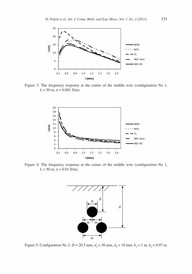
The numerical results for the current induced at the center of the middle wire (confi gura-tion No 1) are shown in Fig. 3. The length of conductors is 50 m and the ground parameters are: s = 0.001 S/m and er = 10.

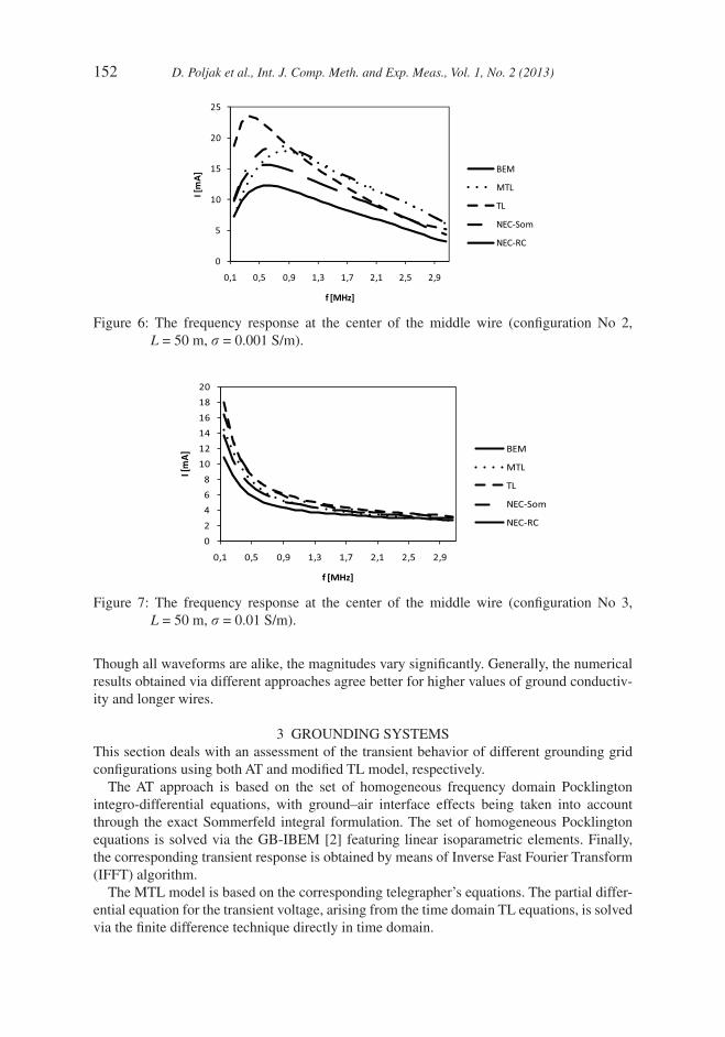
Figure 4 shows the current induced at the center of the middle wire (confi guration No 1) for the conductor length of 50 m with higher ground conductivity (s = 0.01 S/m), while the permittivity is the same (er = 10).

The second confi guration of interest is shown in Fig. 5. The radius of all conductors is 10.25 mm, the distances between neighboring conductors are d1 = 36 mm, d2 = 18 mm, while the burial depths are h1 = 1 m, h2 = 0.97 m.

The numerical results for the current induced at the center of the middle wire (confi gura-tion No 2) are shown in Fig. 6 for the conductor length of 50 m with the conductivity s = 0.001 S/m and permittivity er = 10.

The numerical results for the current induced at the center of the middle wire (confi gura-tion No 2) are shown in Fig. 7 for the conductor length 50 m. The ground parameters are s = 0.01 S/m and er = 10.

D

d d

h

Figure 2: Confi guration No 1: D = 20.5 mm, d = 106 mm, h = 1 m.


02468

101214161820

0,1 0,5 0,9 1,3 1,7 2,1 2,5 2,9

I [m

A]

f [MHz]

BEM

MTL

TL

NEC-Som

NEC-RC

Figure 4: The frequency response at the center of the middle wire (confi guration No 1, L = 50 m, s = 0.01 S/m).

Figure 5: Confi guration No 2: D = 20.5 mm, d1 = 36 mm, d2 = 18 mm, h1 = 1 m, h2 = 0.97 m.

D

d1

h1

h2

d2 d2


0

5

10

15

20

25

0,1 0,5 0,9 1,3 1,7 2,1 2,5 2,9

I [m

A]

f [MHz]

BEM

MTL

TL

NEC-Som

NEC-RC


Though all waveforms are alike, the magnitudes vary signifi cantly. Generally, the numerical results obtained via different approaches agree better for higher values of ground conductiv-ity and longer wires.

3 GROUNDING SYSTEMSThis section deals with an assessment of the transient behavior of different grounding grid confi gurations using both AT and modifi ed TL model, respectively.

The AT approach is based on the set of homogeneous frequency domain Pocklington integro- differential equations, with ground–air interface effects being taken into account through the exact Sommerfeld integral formulation. The set of homogeneous Pocklington equations is solved via the GB-IBEM [2] featuring linear isoparametric elements. Finally, the corresponding transient response is obtained by means of Inverse Fast Fourier Transform (IFFT) algorithm.

The MTL model is based on the corresponding telegrapher’s equations. The partial differ-ential equation for the transient voltage, arising from the time domain TL equations, is solved via the fi nite difference technique directly in time domain.


0

5

10

15

20

25

0,1 0,5 0,9 1,3 1,7 2,1 2,5 2,9

I [m

A]

f [MHz]

BEM

MTL

TL

NEC-Som

NEC-RC


02468

101214161820

0,1 0,5 0,9 1,3 1,7 2,1 2,5 2,9

I [m

A]

f [MHz]

BEM

MTL

TL

NEC-Som

NEC-RC


The physical problem of interest shown in Fig. 8 is related to the square grounding grid energized by a lightning channel.

Several grounding grid confi gurations with dimensions varying from 10 × 10 m2 to 30 × 30 m2, with or without additional vertical electrodes are analyzed in the paper. All grids consist of wire conductors with radius a = 5 mm, and buried at d = 1.5 m depth.

Figure 9 shows various grid confi gurations. Two values of soil conductivity are considered: σ1 = 0.001 S/m and σ2 = 0.01 S/m. In both cases relative permittivity is εr = 9. In all cases the current injection point is located at the center of the grid.

3.1 Antenna theory approach: set of homogeneous Pocklington Integro-differential equations for grounding systems

The currents fl owing along the grounding grid are governed by the set of coupled Pockling-ton integro-differential equations for wires of arbitrary shape [9].

The full wave analysis of grounding systems excited by the current source shown on the left-hand side of expression (25) vanishes and the resulting set of Pocklington equations simplifi es reducing to the homogenous one.

Figure 9: Different grounding grid confi gurations.

10 m 5 m

20 m30 m

10 m

Config. 1 Config. 2

Config. 3Config. 4

Figure 8: Square grounding grid subjected to a lightning stroke.

Injection of the lightning stroke

Square grounding grid

air

earth


( ) ( )

( ) ( )

( ) ( )

21 0

'

2 220 112 2

1 0 1 '

'

' ' , ' '

' * , * ' 0

' * , ' '

1,2,...,

n

W

n

n

n n m n n m n nC

N

n n m n inm m n nn C

n n m n s m n nC

W

I s s s k g s s ds

k kI s s s k g s s ds

k k

I s s s G s s ds

m N

=

⎡ ⎤⎡ ⎤⋅ ⋅ ⋅ + ∇∇ +⎣ ⎦⎢ ⎥⎢ ⎥⎢ ⎥− ⎡ ⎤+ ⋅ ⋅ ⋅ + ∇∇ + =⎢ ⎥⎣ ⎦+⎢ ⎥⎢ ⎥+ ⋅ ⋅ ⋅⎢ ⎥

⎢ ⎥⎣ ⎦=

∫

∑ ∫

∫

� �

� �

� �

(39)

Note that the excitation is taken into account into formulation through the forcing condition [15]:

1 gI I= (40)

where Ig denotes current generator and I1 current at the injection point. Furthermore, at a junction consisting of two or more segments the continuity properties of

the electric fi eld must be satisfi ed [16], which is governed by applying the Kirchhoff current law:

1

0n

kk

I=

=∑ (41)

and the continuity equation:

1 2

1 2' ' 'n

nat junctuion at junctuion at junctuion

II Is s s

⎡ ⎤⎡ ⎤ ⎡ ⎤ ∂∂ ∂= = = ⎢ ⎥⎢ ⎥ ⎢ ⎥∂ ∂ ∂⎣ ⎦ ⎣ ⎦ ⎣ ⎦

� (42)

Condition (42) ensures the discontinuities in charge per unit length to be ruled out in passing from one conductor to another across the junction. On the other hand, at the conductor free ends, the total current vanishes.

3.2 Antenna theory approach: the evaluation of the input impedance spectrum

The input impedance is given by the ratio:

gin

g

VZ

I= (43)

where Vg and Ig are the values of the voltage and the current at the driving point.Once calculating the current distribution, a feeding point voltage is obtained by integrating

the normal electric fi eld component from infi nity to the electrode surface:

r

gV Edl∞

= −∫��

(44)

It is worth noting that the direct calculation of (44) is very time consuming. On the other hand, by carefully choosing an integration path, the computational cost can be appreciably


reduced. Thus, in the case of horizontal arrangement of wires, the best path is vertical, i.e. over the z-axis.

The input impedance spectrum is multiplied with the current spectrum and the frequency response of grounding system is obtained. Finally, the transient response is calculated by means of the IFT.

3.3 Antenna theory approach: numerical solution

The set of Pocklington integro-differential equations (39) is numerically handled via the GB-IBEM. The boundary element solution technique used in this work is an extension of the method applied to single wire cases and presented elsewhere, e.g. in [2].

Undertaking the procedure already presented in Section II.B the set of Pocklington equa-tions (39) is transferred to the system of equations [9]:

[ ] { }i

1 1

= 0, m =1,2,..., ; j =1,2,...,w nN N

en w mji

n i

Z I N N= =

∑∑ (45)

where [Z]ji is the mutual impedance matrix for the j-th observation segment on the m-th antenna and i-th source segment on the n-th antenna, where Nw is the total number of wires, Nm the number of elements on the m-th conductor and Nn the number of segments on the n-th conductor.

Implementation of isoparametric elements yields the following expression for the mutual impedance matrix:

[ ] { } { }

� � { } { }

{ } { }

� � { } { }

1 1

01 1

1 121 0

1 1

1 1

2 21 10 1

2 20 1 2

1

' ( , ' ) ''

' ' ( , ' ) ''

' ( , * ) ''

* ' ( , * ) ''

e T n mnm m nji j i

T n mm n nm m nj i

T n minm m nj i

T nm n inm m nj i

ds dsZ D D g s s d d

d d

ds dsk s s f f g s s d d

d d

ds dsD D g s s d d

d dk kk k ds d

k s s f f g s s dd

z zz z

z zz z

z zz z

zz

− −

− −

− −

= −

+ ⋅ ⋅ +

− +−

++

+ ⋅ ⋅

∫ ∫

∫ ∫

∫ ∫

� � { } { }

1 1

1 1

1 1

1 1

' ' ( , ' ) ''

m

T n mm n snm m nj i

sd

d

ds dss s f f G s s d d

d d

zz

z zz z

− −

− −

⎡ ⎤⎢ ⎥⎢ ⎥ +⎢ ⎥⎢ ⎥⎢ ⎥⎣ ⎦

+ ⋅

∫ ∫

∫ ∫

(46)

Matrices {f} and {f ′} contain the shape functions while {D} and {D ′} contain their derivatives.

The excitation function in the form of the current source Ig is taken into account as a forced condition at the certain node i of the grounding system [9]:

i gI = I (47)

The wire junctions are treated through the Kirchhoff’s current law in its integral and differ-ential form, respectively, related to the continuity of induced currents and charges at the junction (41)–(42).


3.4 Modifi ed transmission line method approach

Within the framework of the MTL approach one neglects the transverse propagation effects the grounding system is simulated by means of a complex network [9].

The corresponding coupling equations for the scalar potential and the current in the time domain for one-dimensional case are reported by the Agrawal model [17]:

( , ) ( , ) ( , ) ( , )s

el

u l t i l tR i l t L E l tl t

∂ ∂+ + =

∂ ∂ (48)

( , ) ( , ) ( , ) 0s

si l t u l tG u l t Cl t

∂ ∂+ + =

∂ ∂ (49)

where l = x or y.El (l, t) is the tangential component of the electric fi eld excitation.Note that combining the two telegrapher’s equations, (48) and (49), the induced current or

voltage can be eliminated and the second order partial differential equation for either voltage or current is obtained. If the propagation occurs in two-directions; x and y, the corresponding two-dimensional partial differential equation for transient voltage is given by:

( )

2 2 2

2 2 22 2 2ees s s sys x

EEu u u uRGu RC LG LCt xx y t y

∂∂∂ ∂ ∂ ∂+ − − + − = +

∂ ∂∂ ∂ ∂ ∂ (50)

where the electric fi eld constitutes the excitation source, and R, L, C and G are per unit length parameters of the interconnected conductors.

For the grounding grid, the per unit length parameters are calculated taking into account the soil–air interface effects. There are various approaches for the assessment of these param-eters, e.g. using the formulas suggested by E.D. Sunde [18] or by Y. Liu [19].

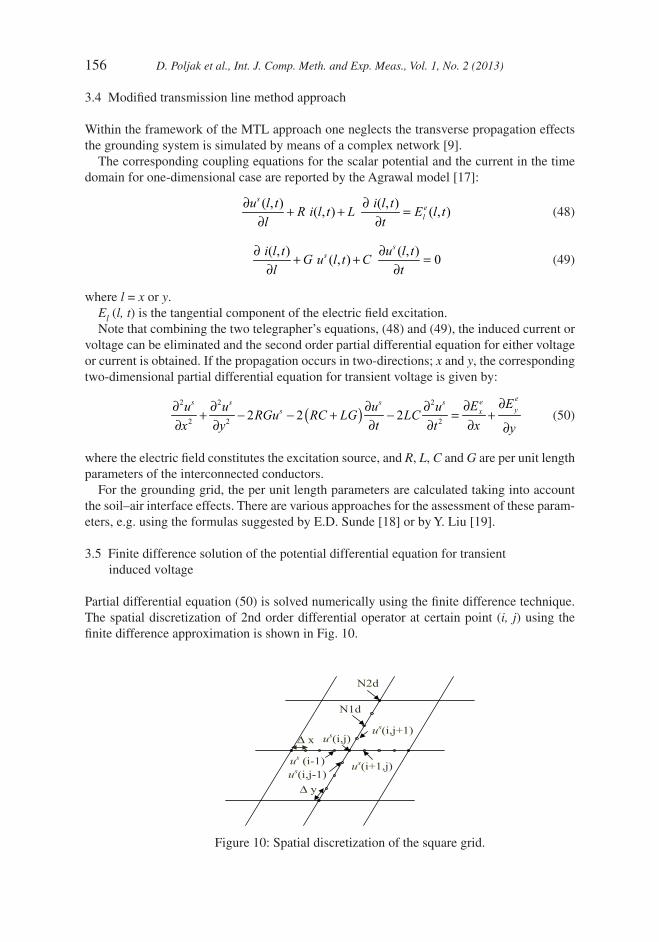
3.5 Finite difference solution of the potential differential equation for transient induced voltage

Partial differential equation (50) is solved numerically using the fi nite difference technique. The spatial discretization of 2nd order differential operator at certain point (i, j) using the fi nite difference approximation is shown in Fig. 10.

N1d

us(i,j-1)us(i+1,j)us (i-1)

us(i,j)Δ x

Δ y

N2d

us(i,j+1)

Figure 10: Spatial discretization of the square grid.


The fi nite difference approximation of spatial and temporal derivatives at certain point (i, j) can be written, as follows:

( ) ( ) ( )

2

2 22

1, , 1,

1sn n ns s su u ui j i j i j

u

x x

⎡ ⎤⎛ ⎞⎢ ⎥− +⎜ ⎟⎢ ⎥+ −⎝ ⎠⎣ ⎦

∂=

∂ Δ (51)

( ) ( ) ( )

2

2 22

, 1 , , 1


u

y y

⎡ ⎤⎢ ⎥− +⎢ ⎥+ −⎣ ⎦

∂=

∂ Δ (52)

( ) ( ) 1

, ,

1s n ns su ui j i j

u t t

⎡ ⎤−⎢ ⎥−⎢ ⎥⎣ ⎦

∂ =∂ Δ

(53)

( ) ( ) ( )

2

22

1 22

, , ,


utt

⎡ ⎤− −⎢ ⎥− +⎢ ⎥⎣ ⎦

∂=

Δ∂ (54)

( ) ( )1, 1,

12

ex n ne eE Ex x

i j i j

Ex x

⎡ ⎤⎢ ⎥−⎢ ⎥+ −⎣ ⎦

∂=

∂ Δ (55)

( ) ( ), 1 , 1

12

ey n ne eE Ey y

i j i j

Ey y

⎡ ⎤⎢ ⎥−⎢ ⎥+ −⎣ ⎦

∂=

∂ Δ (56)

Substituting (51)–(56) into (50) yields the following relation:

( ) ( ) ( ) ( )

( ) ( ) ( ) ( ) ( ) ( )

( ) ( )( )

( )

( ) ( ) ( ) ( )

2 2 2 ,

2 2 21, 1, , 1

1

2 , 1, ,

2

2( ) 42

1, 1,

2 2 2( ) 22

1 1 1

1

2 12

nsi j

n n ns s si j i j i j

n ns si j k i j

s

RC LG LCt t

ne eE Ex xi j i

RC LG LCRG utx y t

u u ux x y

u uy

LC uxt

+ − +

−

−

⎡ ⎤+⎢ ⎥− −⎢ ⎥Δ Δ⎣ ⎦

−+ −

⎤⎡ +− − − − − ⎥⎢ΔΔ Δ Δ ⎥⎢⎣ ⎦

⎡ ⎤ ⎡ ⎤ ⎡ ⎤+ + +⎢ ⎥ ⎢ ⎥ ⎢ ⎥

Δ Δ Δ⎢ ⎥ ⎢ ⎥ ⎢ ⎥⎣ ⎦ ⎣ ⎦ ⎣ ⎦⎡ ⎤

+ =⎢ ⎥Δ⎢ ⎥⎣ ⎦

+ +ΔΔ

( ) ( ) , 1 , 1

12

n

j

n ne eE Ey yi j i j

y

⎡ ⎤⎢ ⎥⎢ ⎥⎣ ⎦

⎡ ⎤⎢ ⎥−⎢ ⎥+ −⎣ ⎦

+Δ

(57)

which can also be expressed in the matrix form:

11 1 1 1 1

1

1

k N

k kk kN k k

N Nk NN N N

A A A U B

A A A U B

A A A U B

⎡ ⎤ ⎡ ⎤ ⎡ ⎤⎢ ⎥ ⎢ ⎥ ⎢ ⎥⎢ ⎥ ⎢ ⎥ ⎢ ⎥⎢ ⎥ ⎢ ⎥ ⎢ ⎥=⎢ ⎥ ⎢ ⎥ ⎢ ⎥⎢ ⎥ ⎢ ⎥ ⎢ ⎥⎢ ⎥ ⎢ ⎥ ⎢ ⎥⎣ ⎦ ⎣ ⎦ ⎣ ⎦

� �

� � � � � � �

� �

� � � � � � �

� �

(58)


where [A] denotes the coeffi cients matrix, [us] is the unknown voltage vector, [B] is the entire right-hand side and N is the total number of nodes.

The diagonal elements of matrix [A] are given by:

( ) ( ) ( )2 2 2

2 2 2( ) 2 2 kkRC LG LCA RG

tx y t+

= − − − − −ΔΔ Δ Δ

(59)

while the non-diagonal elements of matrix [A] are as follows:

( )2

1klA

x=

Δ if 1 is the adjacent node k in x direction (60a)

( )2

1klA

y=

Δ if 1 is the adjacent node k in y direction (60b)

0klA = elsewhere. (60c)

The elements of vector [B] are:

( )( ) ( ) ( )

( ) ( ) ( ) ( )

1 2,

2( ) 42

1, 1, , 1 , 1

2

1 1 2 2

ns sk i j

RC LG LCt t

n n n ne e e eE E E Ex x y yi j i j i j i j

LCB u ut

x y

−⎡ ⎤+⎢ ⎥− −⎢ ⎥Δ Δ⎣ ⎦

⎡ ⎤ ⎡ ⎤⎢ ⎥ ⎢ ⎥− −⎢ ⎥ ⎢ ⎥+ − + −⎣ ⎦ ⎣ ⎦

= + +Δ

+Δ Δ

(61)

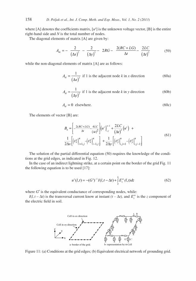
The solution of the partial differential equation (50) requires the knowledge of the condi-tions at the grid edges, as indicated in Fig. 12.

In the case of an indirect lightning strike, at a certain point on the border of the grid Fig. 11 the following equation is to be used [17]:

1( , ) ( ') ( , ) ,h

s esz

0u l t G I l t t E (l t)dz−= − − Δ + ∫ (62)

where G′ is the equivalent conductance of corresponding nodes, while:I(l, t – Δt) is the transversal current know at instant (t – Δt), and es

zE is the z component of the electric fi eld in soil.

L R

G’ C’x

z y

Cell in ox direction

Cell in oy direction

a- border of the grid. b- representation by π-Cell

Figure 11: (a) Conditions at the grid edges; (b) Equivalent electrical network of grounding grid.


The presence of a two-media confi guration is taken into account calculating the linear parameters of the electrical circuit for the case of the grounding electrode [18, 19]. Such a treatment of non-homogeneous media is identical to the case of TL with ground return path.

At each calculation step, the determination of induced voltages provides the evaluation of the currents induced along interconnected conductors of grounding grid by numerical inte-gration of the telegrapher’s equation (48).

Note that the case of the direct impact of the lightning strike on the presented procedure is used by simply imposing Ee = 0. Therefore, in this case the voltage differential equation (eqn (50)) in the frequency domain becomes:

( )

2 2

2 222 0RG j RC LG LC

u u ux y

w w⎡ ⎤+ + −⎢ ⎥⎣ ⎦∂ ∂+ − =∂ ∂

(63)

where u is the potential in any point of the grid.In this case, at the injection node the value of the current is known (lightning strike gener-

ator) providing the assessment of the corresponding voltage.The input impedance is defi ned as follows:

( , )( , )in

u k tZI k t

= (64)

where k is the injection node index.

3.6 Numerical results

In all computational examples the lightning current is expressed by the double exponential function with parameters: I0 = 1.1043 kA, a = 0.07924·106 s–1, b = 0.07924·106 s–1.

Figure 12 shows the transient voltage at the feeding point calculated by AT and TL approach, respectively, for all four grid confi guration scenarios and soil conductivity σ1 = 1 mS/m, while Fig. 13 shows the related transient impedance of the grounding systems.

The results obtained by different approaches for grid type 1 and 2, agree rather satisfacto-rily, and relatively good agreement can be also observed for type 3, while major differences

1 2 3 4 5 6 7 8 9 10x 10–6

05

1015202530354045

|V| (

Vol

t)

t (s)

sigma=0.001AM 1MTL 1AM 2MTL 2AM 3MTL 3AM 4MTL 4

Figure 12: Transient feeding-point voltage for dry soil.


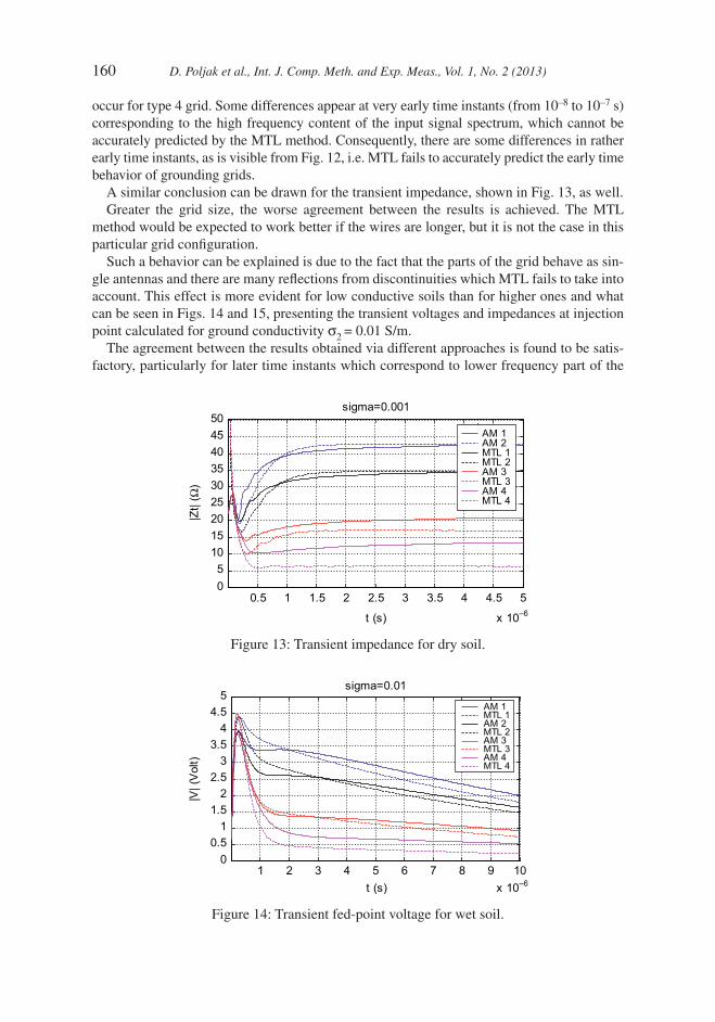
occur for type 4 grid. Some differences appear at very early time instants (from 10–8 to 10–7 s) corresponding to the high frequency content of the input signal spectrum, which cannot be accurately predicted by the MTL method. Consequently, there are some differences in rather early time instants, as is visible from Fig. 12, i.e. MTL fails to accurately predict the early time behavior of grounding grids.

A similar conclusion can be drawn for the transient impedance, shown in Fig. 13, as well. Greater the grid size, the worse agreement between the results is achieved. The MTL

method would be expected to work better if the wires are longer, but it is not the case in this particular grid confi guration.

Such a behavior can be explained is due to the fact that the parts of the grid behave as sin-gle antennas and there are many refl ections from discontinuities which MTL fails to take into account. This effect is more evident for low conductive soils than for higher ones and what can be seen in Figs. 14 and 15, presenting the transient voltages and impedances at injection point calculated for ground conductivity σ2 = 0.01 S/m.

The agreement between the results obtained via different approaches is found to be satis-factory, particularly for later time instants which correspond to lower frequency part of the

Figure 13: Transient impedance for dry soil.

0.5 1 1.5 2 2.5 3 3.5 4 4.5 5

x 10–6

05

101520253035404550

|Zt|

(Ω)

t (s)

sigma=0.001

MTL 1MTL 2AM 3MTL 3AM 4MTL 4

AM 1AM 2

Figure 14: Transient fed-point voltage for wet soil.

1 2 3 4 5 6 7 8 9 10x 10–6

00.5

11.5

22.5

33.5

44.5

5

|V| (

Vol

t)

t (s)

sigma=0.01

AM 1MTL 1AM 2MTL 2AM 3MTL 3AM 4MTL 4


spectrum. For very early time instants the results are alike, although the transient voltage peaks, for all cases of grid confi guration are somewhat higher.

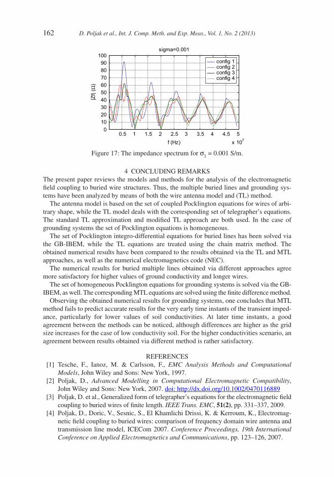
Comparing the results for both values of ground conductivities it can be noticed that the peak value of the voltage is advanced for the case of higher conductivity. Also, the values of the peak voltages are pretty much alike regardless of the grid size. It is well-known that for very early time instants the higher frequency part of the impedance spectrum is important. As the grid density (mesh) remains the same for all grid confi gurations that part of the frequency spectrum is unchanged regardless of the grid size, as shown in Fig. 16. Depending on the conductivity that part of spectrum starts at different frequency values. In the case of σ2 = 0.01 S/m the frequency is about 3 MHz (Fig. 16), while for σ1 = 0.001 S/m it is above 30 MHz (Fig. 17). Thus, one concludes that in high conductivity environment effective length of the grounding wires becomes very short at higher frequencies.

Therefore, very early time behavior is identical for all confi gurations since the very high frequency spectrum part is pretty much the same. Also, it should be noted that the analysis of results presented in Figs. 16 and 17, respectively is related to the results obtained by applying the antenna approach only, as the MTL results are obtained directly in time.

0.5 1 1.5 2 2.5 3 3.5 4 4.5 5x 10–6

02468

101214161820

|Zt|

(Ω)

t (s)

sigma=0.01

AM 1MTL 1AM 2MTL 2AM 3MTL 3AM 4MTL 4

Figure 15: Transient impedance for wet soil.

100 101 102 103 104 105 106 10702468

101214161820

|Zf|

(Ω)

f (Hz)

sigma=0.01

config 1config 2config 3config 4

Figure 16: The impedance spectrum for σ2 = 0.01 S/m.


4 CONCLUDING REMARKSThe present paper reviews the models and methods for the analysis of the electromagnetic fi eld coupling to buried wire structures. Thus, the multiple buried lines and grounding sys-tems have been analyzed by means of both the wire antenna model and (TL) method.

The antenna model is based on the set of coupled Pocklington equations for wires of arbi-trary shape, while the TL model deals with the corresponding set of telegrapher’s equations. The standard TL approximation and modifi ed TL approach are both used. In the case of grounding systems the set of Pocklington equations is homogeneous.

The set of Pocklington integro-differential equations for buried lines has been solved via the GB-IBEM, while the TL equations are treated using the chain matrix method. The obtained numerical results have been compared to the results obtained via the TL and MTL approaches, as well as the numerical electromagnetics code (NEC).

The numerical results for buried multiple lines obtained via different approaches agree more satisfactory for higher values of ground conductivity and longer wires.

The set of homogeneous Pocklington equations for grounding systems is solved via the GB-IBEM, as well. The corresponding MTL equations are solved using the fi nite difference method.

Observing the obtained numerical results for grounding systems, one concludes that MTL method fails to predict accurate results for the very early time instants of the transient imped-ance, particularly for lower values of soil conductivities. At later time instants, a good agreement between the methods can be noticed, although differences are higher as the grid size increases for the case of low conductivity soil. For the higher conductivities scenario, an agreement between results obtained via different method is rather satisfactory.

REFERENCES [1] Tesche, F., Ianoz, M. & Carlsson, F., EMC Analysis Methods and Computational

Models, John Wiley and Sons: New York, 1997. [2] Poljak, D., Advanced Modelling in Computational Electromagnetic Compatibility,

John Wiley and Sons: New York, 2007. doi: http://dx.doi.org/10.1002/0470116889 [3] Poljak, D. et al., Generalized form of telegrapher’s equations for the electromagnetic fi eld

coupling to buried wires of fi nite length. IEEE Trans. EMC, 51(2), pp. 331–337, 2009. [4] Poljak, D., Doric, V., Sesnic, S., El Khamlichi Drissi, K. & Kerroum, K., Electromag-

netic fi eld coupling to buried wires: comparison of frequency domain wire antenna and transmission line model, ICECom 2007. Conference Proceedings, 19th International Conference on Applied Electromagnetics and Communications, pp. 123–126, 2007.

0.5 1 1.5 2 2.5 3 3.5 4 4.5 5x 107

0102030405060708090

100

|Zf|

(Ω)

f (Hz)

sigma=0.001

config 1config 2config 3config 4

Figure 17: The impedance spectrum for σ1 = 0.001 S/m.


[5] Dragan, P., Khalill El Khamlichi, D., Kamal, K. & Silvestar, S., Comparison of analyti-cal and boundary element modeling of electromagnetic fi eld coupling to overhead and buried wires. Engineering Analysis with Boundary Elements, 35(3), pp. 555–563, 2011. doi: http://dx.doi.org/10.1016/j.enganabound.2010.07.010

[6] Poljak, D., Sesnic, S., El-Khamlici Drissi, K. & Kerroum, K., Electromagnetic fi eld coupling to multiple buried thin wires - antenna model versus transmission line approach. Proceedings of EMC Europe 2011 York, 10th International Symposium on Electromagnetic Compatibility, York, EMC Europe, York, pp. 272–277, 2011.

[7] Poljak, D., Doric, V., El Khamlichi Drissi, K., Kerroum, K. & Medic, I., Comparison of wire antenna and modifi ed transmission line approach to the assessment of frequency res-ponse of horizontal grounding electrodes. Engineering Analysis with Boundary Elements, 32(8), pp. 676–681, 2008. doi: http://dx.doi.org/10.1016/j.enganabound.2007.10.019

[8] Poljak, D., Lucic, R., Doric, V. & Antonijevic, S., Frequency domain boundary element versus time domain fi nite element model for the transient analysis of horizontal ground-ing electrode. Engineering Analysis with Boundary Elements, 35(3), pp. 375–382, 2011. doi: http://dx.doi.org/10.1016/j.enganabound.2010.10.001

[9] Cavka, D., Harrat, B., Poljak, D., Nekhoul, B., Kerroum, K. & El Khamlichi Drissi, K., Wire antenna versus modifi ed transmission line approach to the transient analysis of grounding grid. Engineering Analysis with Boundary Elements, 3, pp. 1101–1108, 2011. doi: http://dx.doi.org/10.1016/j.enganabound.2011.05.002

[10] Poljak, D., Cerdic, D., Doric, V., Peratta, A., Roje, V. & Brebbia, C.A., Boundary Element Modeling of Complex Grounding Systems: Study on Current Distribution, BEM 32: Southampton, UK, pp. 123–132, 2010.

[11] Miller, E.K., Poggio, A.J., Burke, G.J. & Selden, E.S., Analysis of wire antennas in the presence of a conducting half-space, part II: the horizontal antenna in free space. Cana-dian Journal of Physics, 50, 2614–2627, 1972. doi: http://dx.doi.org/10.1139/p72-348

[12] Burke, G.J. & Miller, E.K., Modeling antennas near to and penetrating a lossy inter-face. IEEE Trans. on Antenna and Propagation, AP-32(10), pp. 1040–1049, 1984. doi: http://dx.doi.org/10.1109/TAP.1984.1143220

[13] Wallart, J., E. K. Drissi, K. & Paladian, F., Study of propagation constant for a single bur-ied wire in a lossy ground. Proc. EMC ′98 Symposium, vol. 2, Roma, pp. 557–562, 1998.

[14] Burke, G.J., Poggio, A.J., Logan, I.C. & Rockway, J.W., Numerical electromagnet-ics code—a program for antenna system analysis. Int. Symp. Electromagn. Compat., Rotterdam, The Netherlands, 1979.

[15] Grcev, L. & Dawalibi, F., An electromagnetic model for transients in grounding systems. IEEE Trans. Power Delivery, 32(4), pp. 1773–1781, 1990. doi: http://dx.doi.org/10.1109/61.103673

[16] King, R.W.P. & Wu, T.T., Analysis of crossed wires in a plane-wave fi eld. IEEE Trans. on Electromagnetic Compatibility, 17(4), pp. 255–265, 1975. doi: http://dx.doi.org/10.1109/TEMC.1975.303432

[17] Agrawal, A.K., Price, H.J. & Gurbaxani, S.H., Transient response of multiconductor transmission lines excited by a non uniform electromagnetic fi eld. IEEE Trans. On Elec-tromagnetic Compatibility, EMC-22, pp. 119–129, 1980. doi: http://dx.doi.org/10.1109/TEMC.1980.303824

[18] Sunde, E.D., Earth Conducting Effects in Transmission Systems, Dover publications, Inc.: New York, N.Y., 1968.

[19] Liu, Y., Theethayi, N. & Thottappillil, R., An engineering model for transient analysis of grounding system under lightning strikes: nonuniform transmission-line approach. IEEE Trans. on Power Delivery, 20(2), pp. 722–730, 2005. doi: http://dx.doi.org/10.1109/TPWRD.2004.843437

Documents

ELECTROMAGNETIC FIELD COUPLING TO … · Keywords: Buried wires, antenna model, transmission line approximation, set of pocklington integro-differential equations, numerical solution