Electromagnetic and PiezoelectricTransducers

Andre Preumont and Bilal Mokrani

ULB, Active Structures Laboratory,CP. 165-42, 50 Av. F.D. Roosevelt,

B-1050 Brussels, Belgium

Abstract This chapter analyzes the two most popular classes oftransducers used in active vibration control: the electromagnetictransducer known as voice coil, and the piezoelectric transducer.The first part of the chapter discusses the theory of the transduc-ers and the second part discusses some applications in structuralcontrol.

1 Introduction

Transducers are critical in active structures technology; they can play therole of actuator, sensor, or simply energy converter, depending on the appli-cation and the electrical connections. In many applications, the actuatorsare the most critical part of the system; however, the sensors become veryimportant in precision engineering where sub-micron amplitudes must bedetected. This chapter begins with a description of the voice coil transducerand its application to the proof-mass actuator and the geophone (absolutevelocity sensor). The remaining of the chapter is devoted to the piezo-electric materials and the constitutive equations of a discrete piezoelectrictransducer.

2 Voice coil transducer

A voice coil transducer is an energy transformer which converts electricalpower into mechanical power and vice versa. The system consists of a per-manent magnet (Fig.1) which produces a uniform magnetic flux density Bnormal to the gap, and a coil which is free to move axially within the gap.Let v be the velocity of the coil, f the external force acting to maintain thecoil in equilibrium against the electromagnetic forces, e the voltage differ-ence across the coil and i the current into the coil. In this ideal transducer,

1

(b)

Figure 1. Voice-coil transducer: (a) Physical principle. (b) Symbolic rep-resentation.

we neglect the electrical resistance and the self inductance of the coil, aswell as its mass and damping (if necessary, these can be handled by addingR and L to the electrical circuit of the coil, or a mass and damper to itsmechanical model). The voice coil actuator is one of the most popular actu-ators in mechatronics (e.g. it is used in electromagnetic loudspeakers), butit is also used as sensor in geophones.

The first constitutive equation of the voice coil transducer follows fromFaraday’s law : A coil of n turns moving at the velocity v with respect to themagnetic flux density B generates an electromotive force (voltage) e givenby

e = 2πnrBv = Tv (1)

where

T = 2πnrB (2)

is the transducer constant, equal to the product of the length of the coilexposed to the magnetic flux, 2πnr, and the magnetic flux density B. Thesecond equation follows from the Lorentz force law: The external force frequired to balance the total force of the magnetic field on n turns of theconductor is

f = −i 2πnrB = −Ti (3)

2

where i is the current intensity in the coil and T is again the transducerconstant (2). Equation (1) and (3) are the constitutive equations of thevoice coil transducer. Notice that the transducer constant T appearing inFaraday’s law (1), expressed in volt.sec/m, is the same as that appearingin the Lorentz force (3), expressed in N/Amp.

The total power delivered to the moving-coil transducer is equal to thesum of the electric power, ei, and the mechanical power, fv. Combiningwith (1) and (3), one gets

ei+ fv = Tvi− Tiv = 0 (4)

Thus, at any time, there is an equilibrium between the electrical powerabsorbed by the device and the mechanical power delivered (and vice versa).The moving-coil transducer cannot store energy, and behaves as a perfectelectromechanical converter. In practice, however, the transfer is neverperfect due to eddy currents, flux leakage and magnetic hysteresis, leadingto slightly different values of T in (1) and (3).

Let us now examine various applications of the voice coil transducer.

2.1 Proof-mass actuator

A proof-mass actuator (Fig.2) is an inertial actuator which is used invarious applications of vibration control. A reaction mass m is connectedto the support structure by a spring k, a damper c and a force actuatorf which can be either magnetic or hydraulic. In the electromagnetic ac-tuator discussed here, the force actuator consists of a voice coil transducerof constant T excited by a current generator i; the spring is achieved withmembranes which also guide the linear motion of the moving mass. Thesystem is readily modelled as in Fig.2.a. Combining the equation of a singled.o.f. oscillator with the Lorentz force law (3), one finds

mx+ cx+ kx = Ti (5)

or, in the Laplace domain,

x =Ti

ms2 + cs+ k(6)

(s is the Laplace variable). The total force applied to the support is equaland opposite to the force applied to the proof-mass, −mx, or in Laplaceform:

F = −ms2x =−ms2Ti

ms2 + cs+ k(7)

3

Permanentmagnet

Coil

Membranes

Magneticcircuit

Support

Movingmass

Figure 2. Proof-mass actuator (a) model assuming a current generator;(b) conceptual design of an electrodynamic actuator based on a voice coiltransducer. The mass is guided by the membranes.

It follows that the transfer function between the total force F and thecurrent i applied to the coil is

F

i=

−s2T

s2 + 2ξpωps+ ω2p

(8)

where T is the transducer constant (in N/Amp), ωp = (k/m)1/2 is thenatural frequency of the spring-mass system and ξp is the damping ratio,which in practice is fairly high, typically 20 % or more [the negative sign in(8) is irrelevant.] The Bode plots of (8) are shown in Fig.3; one sees that thesystem behaves like a high-pass filter with a high frequency asymptote equalto the transducer constant T ; above some critical frequency ωc ≃ 2ωp, theproof-mass actuator can be regarded as an ideal force generator. It has noauthority over the rigid body modes (at zero frequency) and the operation atlow frequency requires a large stroke, which is technically difficult. Mediumto high frequency actuators (40 Hz and more) are relatively easy to obtainwith low cost components (loudspeaker technology).

If the current source is replaced by a voltage source (Fig.4), the modelingis slightly more complicated and combines the mechanical equation (5) and

4

180

T!p !c

!

iF

Phase

!

Figure 3. Bode plot F/i of an electrodynamic proof-mass actuator (ampli-tude and phase).

an electrical equation which is readily derived from Faraday’s law:

T x+ Ldi

dt+Ri = E(t) (9)

where L is the inductance R is the resistance of the electrical circuit andE(t) is the external voltage source applied to the transducer.

Figure 4. Model of a proof-mass actuator with a voltage source.

5

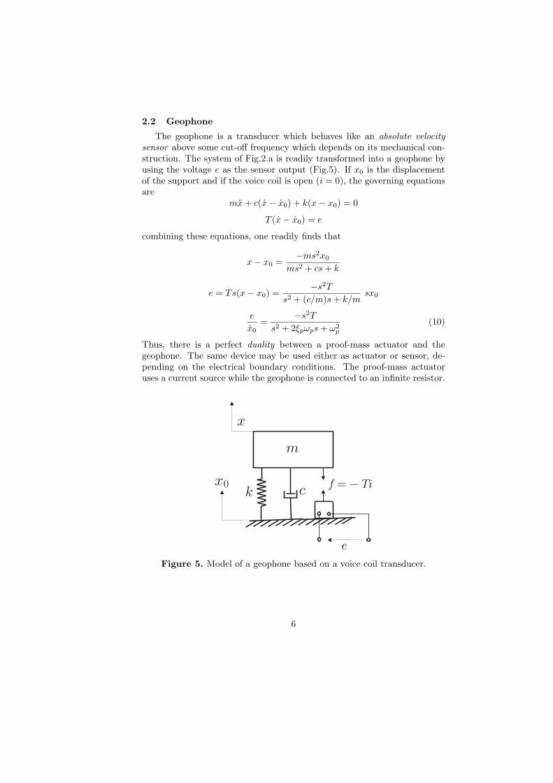
2.2 Geophone

The geophone is a transducer which behaves like an absolute velocitysensor above some cut-off frequency which depends on its mechanical con-struction. The system of Fig.2.a is readily transformed into a geophone byusing the voltage e as the sensor output (Fig.5). If x0 is the displacementof the support and if the voice coil is open (i = 0), the governing equationsare

mx+ c(x− x0) + k(x− x0) = 0

T (x− x0) = e

combining these equations, one readily finds that

x− x0 =−ms2x0

ms2 + cs+ k

e = Ts(x− x0) =−s2T

s2 + (c/m)s+ k/msx0

e

x0=

−s2T

s2 + 2ξpωps+ ω2p

(10)

Thus, there is a perfect duality between a proof-mass actuator and thegeophone. The same device may be used either as actuator or sensor, de-pending on the electrical boundary conditions. The proof-mass actuatoruses a current source while the geophone is connected to an infinite resistor.

x0

e

Figure 5. Model of a geophone based on a voice coil transducer.

6

Above the corner frequency, the gain of the geophone is equal to the trans-ducer constant T . Designing geophones with very low corner frequency isin general difficult, especially if their orientation with respect to the gravityvector is variable; active geophones where the corner frequency is loweredelectronically may constitute a good alternative option.

3 General electromechanical transducer

3.1 Constitutive equations

The constitutive behavior of a wide class of electromechanical transduc-ers can be modeled as in Fig.6, where the central box represents the conver-sion mechanism between electrical energy and mechanical energy, and viceversa. In Laplace form, the constitutive equations read

Tme

Teme

Zei Zm v = xç

f

Figure 6. Electrical analog representation of an electromechanical trans-ducer.

e = Zei+ Temv (11)

f = Tmei+ Zmv (12)

where e is the Laplace transform of the input voltage across the electricalterminals, i the input current, f the force applied to the mechanical termi-nals, and v the velocity of the mechanical part. Ze is the blocked electricalimpedance, measured for v = 0; Tem is the transduction coefficient repre-senting the electromotive force (voltage) appearing in the electrical circuitper unit velocity in the mechanical part (in volt.sec/m). Tme is the trans-duction coefficient representing the force acting on the mechanical terminalsto balance the electromagnetic force induced per unit current input on theelectrical side (in N/Amp), and Zm is the mechanical impedance, measuredwhen the electrical side is open (i = 0).

To illustrate this representation, consider the proof-mass actuator withthe voltage source of Fig.4; the electrical equation reads

E(t) = Ri+ Ldi

dt+ Tv

7

or in Laplace formE = (Ls+R)i+ Tv

If F is the external force applied to the mechanical terminal (positive in thepositive direction of v), the mechanical equation reads

F (t) = mx+ cx+ kx− Ti

or in Laplace form (using the velocity as mechanical variable)

F = (ms+ c+ k/s)v − Ti

Thus, the constitutive equations may be written in the form (11) and (12)with

Ze = Ls+R, Zm = ms+ c+ k/s, Tem = T, Tme = −T

In absence of external force (f = 0), v can be resolved from Equ.(12)and substituted into Equ.(11), leading to

e = (Ze −TemTme

Zm)i

−TemTme/Zm is called the motional impedance. The total driving pointelectrical impedance is the sum of the blocked and the motional impedances.

3.2 Self-sensing

Equation (11) shows that the voltage drop across the electrical terminalsof any electromechanical transducer is the sum of a contribution propor-tional to the current applied and a contribution proportional to the velocityof the mechanical terminals. Thus, if Zei can be measured and subtractedfrom e, a signal proportional to the velocity is obtained. This suggeststhe bridge structure of Fig.7. The bridge equations are as follows: for thebranch containing the transducer,

e = ZeI + Temv + ZbI

I =1

Ze + Zb(e− Temv)

V4 = ZbI =Zb

Ze + Zb(e− Temv)

For the other branch,e = kZei+ kZbi

8

Transducer

Figure 7. Bridge circuit for self-sensing actuation.

V2 = kZbi =Zb

Ze + Zbe

and the bridge output

V4 − V2 = (−Zb Tem

Ze + Zb) v (13)

is indeed a linear function of the velocity v of the mechanical terminals.Note, however, that −Zb Tem/(Ze+Zb) acts as a filter; the bridge impedanceZb must be adapted to the transducer impedance Ze to avoid amplitude dis-tortion and phase shift between the output voltage V4 − V2 and the trans-ducer velocity in the frequency band of interest.

4 Smart materials

Piezoelectric materials belong to the so-called smart materials, or multi-functional materials, which have the ability to respond significantly to stim-uli of different physical natures. Figure 8 lists various effects that are ob-served in materials in response to various inputs: mechanical, electrical,magnetic, thermal, light. The coupling between the physical fields of differ-ent types is expressed by the non-diagonal cells in the figure; if its magnitudeis sufficient, the coupling can be used to build discrete or distributed trans-ducers of various types, which can be used as sensors, actuators, or evenintegrated in structures with various degrees of tailoring and complexity

9

Input

OutputStrain

Electric

charge

Magnetic

fluxTemperature Light

Stress

Electric

field

Elasticity

Heat

Light

Permittivity

Piezo-

electricity

Piezo-

electricity

Magneto-

striction

Magneto-

strictionMagnetic

field

Thermal

expansion

Photostriction

Magneto-

electric

effect

Pyro-

electricity

Photo-

voltaic

effect

Permeability

Specific

heat

Refractive

index

Magneto

-optic

Electro

-optic

effect

Photo-

elasticity

Figure 8. Stimulus-response relations indicating various effects in materi-als. The smart materials correspond to the non-diagonal cells.

(e.g. as fibers), to make them controllable or responsive to their environ-ment (e.g. for shape morphing, precision shape control, damage detection,dynamic response alleviation,...).

Figure 9 summarizes the mechanical properties of a few smart mate-rials which are considered for actuation in structural control applications.Figure 9.a shows the maximum (blocked) stress versus the maximum (free)strain; the diagonal lines in the diagram indicate a constant energy density.Figure 9.b shows the specific energy density (i.e. energy density by unitmass) versus the maximum frequency; the diagonal lines indicate a con-stant specific power density. Note that all the material characteristics varyby several orders of magnitude. Among them all, the piezoelectric materialsare undoubtedly the most mature and those with the most applications.

5 Piezoelectric transducer

The piezoelectric effect was discovered by Pierre and Jacques Curie in 1880.The direct piezoelectric effect consists in the ability of certain crystallinematerials to generate an electrical charge in proportion to an externallyapplied force; the direct effect is used in force transducers. According to

10

Strain (%)

Frequency (Hz)

10à2

10à1

100

101

102

103

100

101

102

103

104

105

Str

ess

(M

Pa)

Spe

cifi

c E

nerg

y D

ens

ity

(J/k

g)

101100 102 103 104 105 106

10à2 10à1 101100 102 103

10 J/m³

10² J/m³

10³ J/m³

10 J/m³

4

10J/m³

5

10J/m³

6

10J/m³

8

10J/m³

9Energy Density

Single Crystal

PZT

PZT

Electrostrictive

polymer

PVDFElectrostatic

device

Voice Coil

Magneto-

strictive

Nanotube

Dielectric

Elastomer

(Silicon)

Dielectric

Elastomer

(Acryl)

Ionic

Polymer

Metal

Composite

Responsive

Gels

Thermal

Shape Memory

Polymer

Conducting Polymer

Shape Memory Alloy

PZTSingle Crystal

PZT

Electrostrictive polymer

Electrostatic

device

Voice Coil

Magneto-

strictiveNanotube

Dielectric

Elastomer

(Silicon)

Dielectric

Elastomer

(Acryl)

Ionic

Polymer

Metal

CompositeResponsive

Gels

Thermal

Shape Memory

Polymer

Conducting Polymer

Shape Memory Alloy

Muscle

PVDF

10 W/kg (Muscle)

DC-Motor

10³ W/kg

10W

/kg

5

10W

/kg

7

Specific Power Density

10W

/kg

9

Figure 9. (a) Maximum stress vs. maximum strain of various smart ma-terial actuators. (b) Specific energy density vs. maximum frequency (bycourtesy of R.Petricevic, Neue Materialen Wurzburg).

11

the inverse piezoelectric effect, an electric field parallel to the direction ofpolarization induces an expansion of the material. The piezoelectric effectis anisotropic; it can be exhibited only by materials whose crystal structurehas no center of symmetry; this is the case for some ceramics below a cer-tain temperature called the Curie temperature; in this phase, the crystalhas built-in electric dipoles, but the dipoles are randomly orientated andthe net electric dipole on a macroscopic scale is zero. During the polingprocess, when the crystal is cooled in the presence of a high electric field,the dipoles tend to align, leading to an electric dipole on a macroscopicscale. After cooling and removing of the poling field, the dipoles cannotreturn to their original position; they remain aligned along the poling di-rection and the material body becomes permanently piezoelectric, with theability to convert mechanical energy to electrical energy and vice versa; thisproperty will be lost if the temperature exceeds the Curie temperature orif the transducer is subjected to an excessive electric field in the directionopposed to the poling field.

The most popular piezoelectric materials are Lead-Zirconate-Titanate(PZT) which is a ceramic, and Polyvinylidene fluoride (PVDF) which is apolymer. In addition to the piezoelectric effect, piezoelectric materials ex-hibit a pyroelectric effect, according to which electric charges are generatedwhen the material is subjected to temperature; this effect is used to produceheat detectors; it will not be discussed here.

In this section, we consider a transducer made of a one-dimensionalpiezoelectric material of constitutive equations (we use the notations of theIEEE Standard on Piezoelectricity)

D = εTE + d33T (14)

S = d33E + sET (15)

where D is the electric displacement (charge per unit area, expressed inCoulomb/m2), E the electric field (V/m), T the stress (N/m2) and S thestrain. εT is the dielectric constant (permittivity) under constant stress,sE is the compliance when the electric field is constant (inverse of theYoung’s modulus) and d33 is the piezoelectric constant, expressed in m/Vor Coulomb/Newton; the reason for the subscript 33 is that, by convention,index 3 is always aligned to the poling direction of the material, and weassume that the electric field is parallel to the poling direction. Note thatthe same constant d33 appears in (14) and (15).

12

In the absence of an external force, a transducer subjected to a voltagewith the same polarity as that during poling produces an elongation, and avoltage opposed to that during poling makes it shrink (inverse piezoelectriceffect). In (15), this amounts to a positive d33. Conversely (direct piezo-electric effect), if we consider a transducer with open electrodes (D = 0),

according to (14), E = −(d33/εT)T , which means that a traction stress will

produce a voltage with polarity opposed to that during poling, and a com-pressive stress will produce a voltage with the same polarity as that duringpoling.

5.1 Constitutive relations of a discrete transducer

Equations (14) and (15) can be written in a matrix formDS

=

[εT d33d33 sE

]ET

(16)

where (E, T ) are the independent variables and (D, S) are the dependentvariables. If (E, S) are taken as the independent variables, they can berewritten

D =d33sE

S + εT(1− d33

2

sEεT

)E

T =1

sES − d33

sEE

or DT

=

[εT (1− k2) e33

−e33 cE

]ES

(17)

where cE = 1/sE is the Young’s modulus under E = 0 (short circuited elec-trodes), in N/m2 (Pa); e33 = d33/s

E , the product of d33 by the Youngmodulus, is the constant relating the electric displacement to the strain forshort-circuited electrodes (in Coulomb/m2), and also that relating the com-pressive stress to the electric field when the transducer is blocked (S = 0).

k2 =d33

2

sEεT=

e332

cEεT(18)

k is called the Electromechanical coupling factor of the material; it measuresthe efficiency of the conversion of mechanical energy into electrical energy,and vice versa, as discussed below. From (17), we note that εT (1− k2) isthe dielectric constant under zero strain.

13

+_

Cross section:Thickness:

# of disks in the stack:

Electric charge:

Capacitance:

At

nl = nt

Q = nAD

Electrode

Free piezoelectric expansion:Voltage driven:

Charge driven:

î = d33nV

î = d33nCQ

t

E = V=t

C = n2"A=l

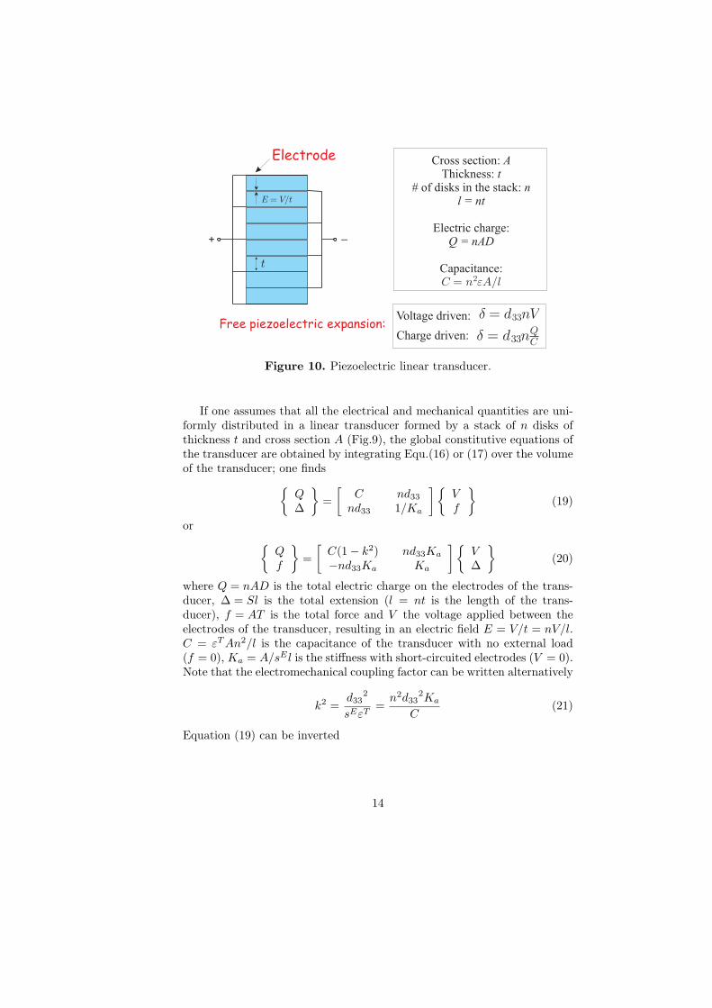
Figure 10. Piezoelectric linear transducer.

If one assumes that all the electrical and mechanical quantities are uni-formly distributed in a linear transducer formed by a stack of n disks ofthickness t and cross section A (Fig.9), the global constitutive equations ofthe transducer are obtained by integrating Equ.(16) or (17) over the volumeof the transducer; one finds

Q∆

=

[C nd33

nd33 1/Ka

]Vf

(19)

or Qf

=

[C(1− k2) nd33Ka

−nd33Ka Ka

]V∆

(20)

where Q = nAD is the total electric charge on the electrodes of the trans-ducer, ∆ = Sl is the total extension (l = nt is the length of the trans-ducer), f = AT is the total force and V the voltage applied between theelectrodes of the transducer, resulting in an electric field E = V/t = nV/l.C = εTAn2/l is the capacitance of the transducer with no external load(f = 0), Ka = A/sEl is the stiffness with short-circuited electrodes (V = 0).Note that the electromechanical coupling factor can be written alternatively

k2 =d33

2

sEεT=

n2d332Ka

C(21)

Equation (19) can be inverted

14

Vf

=

Ka

C(1− k2)

[1/Ka −nd33−nd33 C

]Q∆

(22)

from which we can see that the stiffness with open electrodes (Q = 0) isKa/(1−k2) and the capacitance for a fixed geometry (∆ = 0) is C(1− k2).Note that typical values of k are in the range 0.3− 0.7; for large k, thestiffness changes significantly with the electrical boundary conditions, andsimilarly the capacitance depends on the mechanical boundary conditions.

Next, let us write the total stored electromechanical energy and coenergyfunctions.1 Consider the discrete piezoelectric transducer of Fig.11; the

Figure 11. Discrete Piezoelectric transducer.

total power delivered to the transducer is the sum of the electric power, V iand the mechanical power, f∆. The net work on the transducer is

dW = V idt+ f∆dt = V dQ+ fd∆ (23)

For a conservative element, this work is converted into stored energy, dWe,and the total stored energy, We(∆, Q) can be obtained by integrating (23)from the reference state to the state (∆, Q).2 Upon differentiatingWe(∆, Q),

dWe(∆, Q) =∂We

∂∆d∆+

∂We

∂QdQ (24)

1Energy and coenergy functions are needed in connection with energy formulations such

as Hamilton principle, Lagrange equations or finite elements.2Since the system is conservative, the integration can be done along any path leading

from (0, 0) to (∆, Q).

15

and, comparing with (23), we recover the constitutive equations

f =∂We

∂∆V =

∂We

∂Q(25)

Substituting f and V from (22) into (23), one gets

dWe = V dQ+ fd∆

=QdQ

C(1− k2)− nd33Ka

C(1− k2)(∆ dQ+Qd∆) +

Ka

1− k2∆ d∆

which is the total differential of

We(∆, Q) =Q2

2C(1− k2)− nd33Ka

C(1− k2)Q∆+

Ka

1− k2∆2

2(26)

This is the analytical expression of the stored electromechanical energy forthe discrete piezoelectric transducer. The partial derivatives (25) allow torecover the constitutive equations (22). The first term on the right handside of (26) is the electrical energy stored in the capacitance C(1− k2)(corresponding to a fixed geometry, = 0); the third term is the elasticstrain energy stored in a spring of stiffness Ka/(1 − k2) (corresponding toopen electrodes, Q = 0); the second term is the piezoelectric energy.

The electromechanical energy function uses ∆ and Q as independentstate variables. A coenergy function using ∆ and V as independent variablescan be defined by the Legendre transformation

W ∗e (∆, V ) = V Q−We(∆, Q) (27)

The total differential of the coenergy is

dW ∗e = QdV + V dQ− ∂We

∂∆d∆− ∂We

∂QdQ

dW ∗e = QdV − f d∆ (28)

where Equ.(25) have been used. It follows that

Q =∂W ∗

e

∂Vand f = −∂W ∗

e

∂∆(29)

Introducing the constitutive equations (20) into (28),

dW ∗e =

[C(1− k2)V + nd33Ka∆

]dV + (nd33KaV −Ka∆) d∆

= C(1− k2)V dV + nd33Ka (∆dV + V d∆)−Ka∆ d∆

16

which is the total differential of

W ∗e (∆, V ) = C(1− k2)

V 2

2+ nd33KaV∆−Ka

∆2

2(30)

This is the analytical form of the coenergy function for the discrete piezoelec-tric transducer. The first term on the right hand side of (30) is recognizedas the electrical coenergy in the capacitance C(1− k2) (corresponding toa fixed geometry, ∆ = 0); the third is the strain energy stored in a springof stiffness Ka (corresponding to short-circuited electrodes, V = 0). Thesecond term of (30) is the piezoelectric coenergy; using the fact that theuniform electric field is E = nV/l and the uniform strain is S = ∆/l, it canbe rewritten ∫

Ω

Se33E dΩ (31)

where the integral extends to the volume Ω of the transducer.The analytical form (26) of the electromechanical energy, together with

the constitutive equations (25) can be regarded as an alternative defini-tion of a discrete piezoelectric transducer, and similarly for the analyticalexpression of the coenergy (30) and the constitutive equations (29).

5.2 Interpretation of k2

Consider a piezoelectric transducer subjected to the following mechanicalcycle: first, it is loaded with a force F with short-circuited electrodes; theresulting extension is

∆1 =F

Ka

where Ka = A/(sEl) is the stiffness with short-circuited electrodes. Theenergy stored in the system is

W1 =

∫ ∆1

0

f dx =F∆1

2=

F 2

2Ka

At this point, the electrodes are open and the transducer is unloaded ac-cording to a path of slope Ka/(1− k2), corresponding to the new electricalboundary conditions,

∆2 =F (1− k2)

Ka

The energy recovered in this way is

W2 =

∫ ∆2

0

f dx =F∆2

2=

F 2(1− k2)

2Ka

17

leaving W1−W2 stored in the transducer. The ratio between the remainingstored energy and the initial stored energy is

W1 −W2

W1= k2

Similarly, consider the following electrical cycle: first, a voltage V isapplied to the transducer which is mechanically unconstrained (f = 0).The electric charges appearing on the electrodes are

Q1 = CV

where C = εTAn2/l is the unconstrained capacitance, and the energy storedin the transducer is

W1 =

∫ Q1

0

v dq =V Q1

2=

CV 2

2

At this point, the transducer is blocked mechanically [changing its capac-itance from C to C(1 − k2)] and electrically unloaded from V to 0. Theelectrical charges are removed according to

Q2 = C(1− k2)V

The energy recovered in this way is

W2 =

∫ Q2

0

v dq =C(1− k2)V 2

2

leaving W1 − W2 stored in the transducer. Here again, the ratio betweenthe remaining stored energy and the initial stored energy is

W1 −W2

W1= k2

Although the foregoing relationships provide a clear physical interpretationof the electromechanical coupling factor, they do not bring a practical wayof measuring k2; the experimental determination of k2 is often based onimpedance (or admittance) measurements.

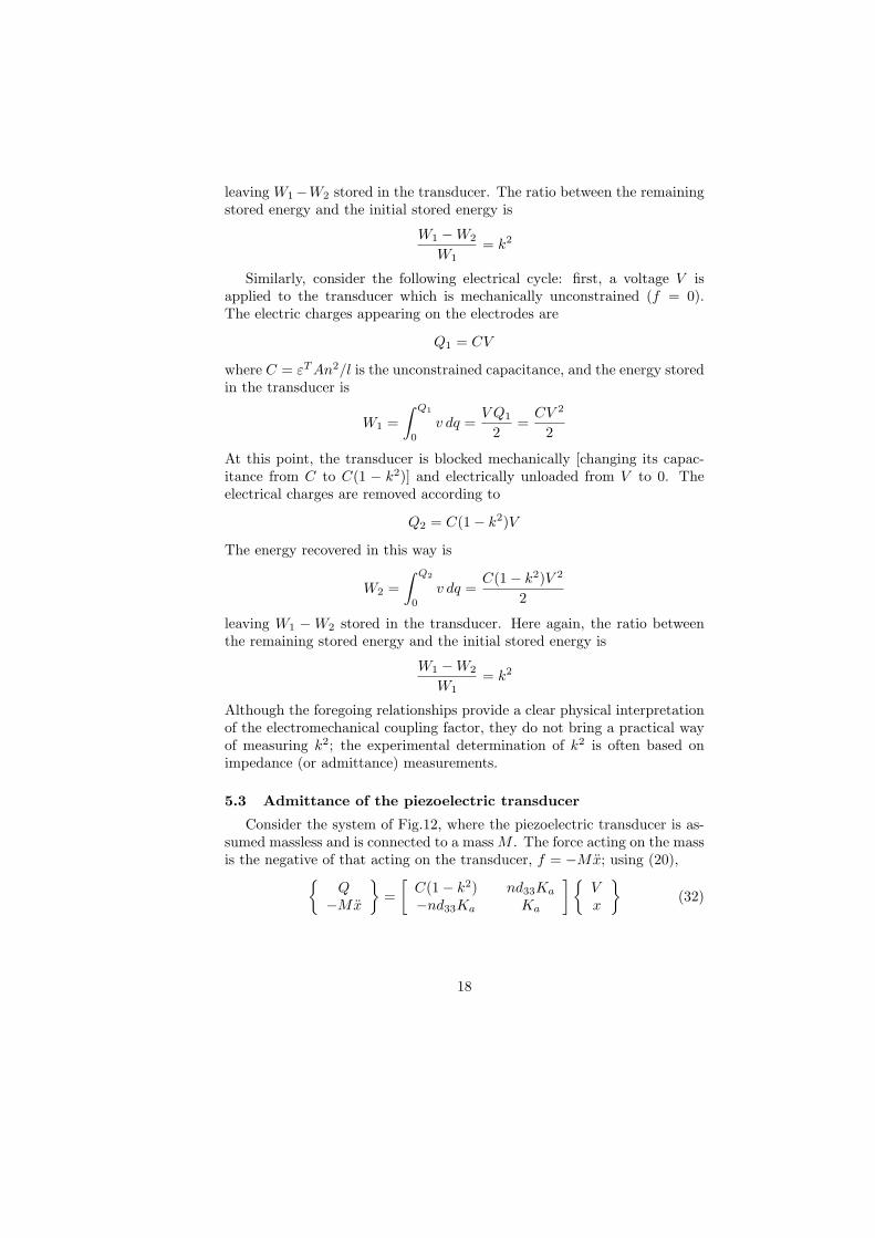
5.3 Admittance of the piezoelectric transducer

Consider the system of Fig.12, where the piezoelectric transducer is as-sumed massless and is connected to a mass M . The force acting on the massis the negative of that acting on the transducer, f = −Mx; using (20),

Q−Mx

=

[C(1− k2) nd33Ka

−nd33Ka Ka

]Vx

(32)

18

(a)

Transducer

dB

(b)

Figure 12. (a) Elementary dynamical model of the piezoelectric transducer.(b) Typical admittance FRF of the transducer, in the vicinity of its naturalfrequency.

From the second equation, one gets (in Laplace form)

x =nd33Ka

Ms2 +KaV

and, substituting in the first one and using (21), one finds

Q

V= C(1− k2)

[Ms2 +Ka/(1− k2)

Ms2 +Ka

](33)

It follows that the admittance reads:

I

V=

sQ

V= sC(1− k2)

s2 + z2

s2 + p2(34)

where the poles and zeros are respectively

p2 =Ka

Mand z2 =

Ka/(1− k2)

M(35)

p is the natural frequency with short-circuited electrodes (V = 0) and zis the natural frequency with open electrodes (I = 0). From the previousequation one sees that

z2 − p2

z2= k2 (36)

This relationship constitutes a practical way of determining the electrome-chanical coupling factor: An impedance meter is used to measure the Fre-quency Response Function (FRF) of the admittance (or the impedance), on

19

which the position of the poles p and zeros z are identified and introducedin Equ.(36).

6 Vibration isolation with voice coil transducers

6.1 Viscous damping isolator

Consider the spring mass system of Fig.13. A voice coil connects themassM to the moving support and a resistor R is connected to the electricalterminals of the voice coil. The governing equations are

Voice coil

Figure 13. Voice coil used as viscous damper.

Mx+ k(x− x0) = Ti

e = −Ri = Tv = T (x− x0)

where the constitutive equations of the voice coil [Equ.(1) and (3)] havebeen used. Upon eliminating i between these equations, one finds

Mx+T 2

R(x− x0) + k(x− x0) = 0 (37)

Thus, when a resistor connects the electrical terminals of the voice coil,it behaves as a viscous damper of damping coefficient c = T 2/R; a lowerresistance R will increase the damping (the minimum value of R is thatof the coil itself). From the foregoing equation, the transmissibility of theisolator is readily obtained:

X

X0=

1 + 2jξω/ωn

1 + 2jξω/ωn − ω2/ω2n

(38)

20

0

xx

0 = 0

1

2 1>

101 2

n

10

-10

0.1

-20

dB

w-2

w-1

Figure 14. Transmissibility of the passive isolator for various values of thedamping ratio ξ. The high frequency decay rate is ω−1.

with the usual notations ω2n = k/M and 2ξωn = c/M . It is displayed

in Fig.14 for various values of the damping ratio ξ: (i) All the curves arelarger than 1 for ω <

√2 ωn and become smaller than 1 for ω >

√2 ωn.

Thus the critical frequency√2 ωn separates the domains of amplification

and attenuation of the isolator. (ii) When ξ = 0, the high frequency decayrate is ω−2, that is -40 dB/decade, while very large amplitudes occur nearthe corner frequency ωn (the natural frequency of the spring-mass system).

Figure 14 illustrates the trade-off in passive isolator design: large damp-ing is desirable at low frequency to reduce the resonant peak while lowdamping is needed at high frequency to maximize the isolation. One ob-serves that if the disturbance is generated by a rotating unbalance of amotor with variable speed, there is an obvious benefit to use a damper withvariable damping characteristics which can be adjusted according to therotation velocity: high damping when ω <

√2ωn and low damping when

ω >√2ωn. Such (adaptive) devices can be readily obtained with a variable

resistor R. The following section discusses another electrical circuit whichimproves the high frequency decay rate of the isolator.

21

6.2 Relaxation isolator

Voice coil

Figure 15. (a) Relaxation isolator. (b) Electromagnetic realization.

In the relaxation isolator, the viscous damper c is replaced by a Maxwellunit consisting of a damper c and a spring k1 in series (Fig.15.a). Thegoverning equations are

Mx+ k(x− x0) + c(x− x1) = 0 (39)

c(x− x1) = k1(x1 − x0) (40)

or, in matrix form using the Laplace variable s,[Ms2 + cs+ k −cs

−cs k1 + cs

]xx1

=

kk1

x0 (41)

Upon inverting this system of equations, the transmissibility is obtained inLaplace form:

x

x0=

(k1 + cs)k + k1cs

(Ms2 + cs+ k)(k1 + cs)− c2s2=

(k1 + cs)k + k1cs

(Ms2 + k)(k1 + cs) + k1cs(42)

One sees that the asymptotic decay3 rate for large frequencies is in s−2,that is -40 dB/decade. Physically, this corresponds to the fact that, at high

3the asymptotic decay rate is governed by the largest power of s of the numerator and

the denominator.

22

1 10

-40

-20

0

!=!n

xx

0dBc = 0 c!1

copt

A

Figure 16. Transmissibility of the relaxation oscillator for fixed values ofk and k1 and various values of c. The first peak corresponds to ω = ωn =(k/M)1/2; the second one corresponds to ω = Ωn = [(k + k1)/M ]1/2. Allthe curves cross each other at A and have an asymptotic decay rate of -40dB/decade. The curve corresponding to copt is nearly maximum at A.

frequency, the viscous damper tends to be blocked, and the system behaveslike an undamped isolator with two springs acting in parallel. Figure 16compares the transmissibility curves for given values of k and k1 and variousvalues of c. For c = 0, the relaxation isolator behaves like an undampedisolator of natural frequency ωn = (k/M)1/2. Likewise, for c → ∞, itbehaves like an undamped isolator of frequency Ωn = [(k + k1)/M ]1/2. Inbetween, the poles of the system are solution of the characteristic equation

(Ms2 + k)(k1 + cs) + k1cs = (Ms2 + k)k1 + cs(Ms2 + k + k1) = 0

which can be rewritten in root locus form

1 +k1c

s2 + ω2n

s(s2 +Ω2n)

= 0 (43)

It is represented in Fig.17 when c varies from 0 to ∞; it can be shown that

23

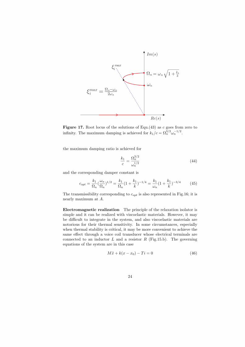
Figure 17. Root locus of the solutions of Equ.(43) as c goes from zero to

infinity. The maximum damping is achieved for k1/c = Ω3/2n ω

−1/2n .

the maximum damping ratio is achieved for

k1c

=Ω

3/2n

ω1/2n

(44)

and the corresponding damper constant is

copt =k1Ωn

(ωn

Ωn)1/2 =

k1Ωn

(1 +k1k)−1/4 =

k1ωn

(1 +k1k)−3/4 (45)

The transmissibility corresponding to copt is also represented in Fig.16; it isnearly maximum at A.

Electromagnetic realization The principle of the relaxation isolator issimple and it can be realized with viscoelastic materials. However, it maybe difficult to integrate in the system, and also viscoelastic materials arenotorious for their thermal sensitivity. In some circumstances, especiallywhen thermal stability is critical, it may be more convenient to achieve thesame effect through a voice coil transducer whose electrical terminals areconnected to an inductor L and a resistor R (Fig.15.b). The governingequations of the system are in this case

Mx+ k(x− x0)− Ti = 0 (46)

24

Ldi

dt+ T (x− x0) +Ri = 0 (47)

where T is the transducer constant. In matrix form, using the Laplacevariable, [

Ms2 + k −TTs Ls+R

]xi

=

kTs

x0 (48)

It follows that the transmissibility reads

x

x0=

(Ls+R)k + T 2s

(Ms2 + k)(Ls+R) + T 2s(49)

Comparing with Equ.(42), one sees that the electromechanical isolator be-haves exactly like a relaxation isolator provided that

Ls+R

T 2=

cs+ k1k1c

(50)

or

k1 =T 2

Lc =

T 2

R(51)

These are the two relationships between the three parameters T , L and Rso that the transmissibility of the electromechanical system of Fig.15.b isthe same as that of Fig.15.a.

7 Controlling structures with piezo transducers

Consider a structure with a single discrete piezoelectric transducer (Fig.18);the transducer is governed by Equ.(20):

Qf

=

[C(1− k2) nd33Ka

−nd33Ka Ka

]VbTx

(52)

where ∆ = bTx is the relative displacement at the extremities of the trans-ducer. The dynamics of the structure is governed by

Mx+K∗x = −bf (53)

where K∗ is the stiffness matrix of the structure without the transducer andb is the influence vector of the transducer in the global coordinate system ofthe structure. The non-zero components of b are the direction cosines of theactive bar. The minus sign on the right hand side of the previous equationcomes from the fact that the force acting on the structure is opposed tothat acting on the transducer. Note that the same vector b appears in both

25

I

VPiezoelectric

Transducer

Structure

D = b xT

f

M K, *

Figure 18. Structure with a piezoelectric transducer. b is the influencevector of the transducer in the global coordinate system of the structure.

equations because the relative displacement is measured along the directionof f . Substituting f from the constitutive equation into the second equation,one finds

Mx+ (K∗ + bbTKa)x = bKand33V

or

Mx+Kx = bKaδ (54)

where K = K∗ + bbTKa is the global stiffness matrix of the structureincluding the piezoelectric transducer in short-circuited conditions (whichcontributes for bbTKa); δ = nd33V is the free expansion of the transducerinduced by a voltage V ; Kaδ is the equivalent piezoelectric loading: theeffect of the piezoelectric transducer on the structure consists of a pair ofself-equilibrating forces applied axially to the ends of the transducer; as forthermal loads, their magnitude is equal to the product of the stiffness of thetransducer (in short-circuited conditions) by the unconstrained piezoelectricexpansion; this is known as the thermal analogy.

Let ϕi be the normal modes, solutions of the eigenvalue problem

(K − ω2iM)ϕi = 0 (55)

They satisfy the usual orthogonality conditions

ϕTi Mϕj = µiδij (56)

ϕTi Kϕj = µiω

2i δij (57)

26

where ωi is the natural frequency when the transducer is short-circuited. Ifthe global displacements are expanded into modal coordinates,

x =∑i

ziϕi (58)

where zi are the modal amplitudes, Equ.(54) is easily transformed into

µi(zi + ω2i zi) = ϕT

i bKaδ (59)

Upon taking the Laplace transform, one easily gets

x =

n∑i=1

ϕiϕTi

µi(ω2i + s2)

bKaδ (60)

and the transducer extension

∆ = bTx =n∑

i=1

Ka(bTϕi)

2

µiω2i (1 + s2/ω2

i )δ (61)

From Equ.(57), µiω2i /2 is clearly the strain energy in the structure when it

vibrates according to mode i, and Ka(bTϕi)

2/2 represents the strain energyin the transducer when the structure vibrates according to mode i. Thus,the ratio

νi =Ka(b

Tϕi)2

µiω2i

(62)

is readily interpreted as the fraction of modal strain energy in the transducerfor mode i. With this notation, the previous equation is rewritten

∆ = bTx =n∑

i=1

νi(1 + s2/ω2

i )δ (63)

which relates the actual displacement of the transducer with the free ex-pansion due to the voltage V .

7.1 Force feedback open-loop transfer function

A frequent control configuration is that of an active strut where thepiezoelectric actuator is coupled with a collocated force sensor. From thesecond constitutive equation (52), the open-loop transfer function betweenthe free expansion δ = nd33V of the transducer (proportional to the appliedvoltage) and the output force f in the active strut is readily obtained:

f = −Kaδ +Ka∆

27

Figure 19. (a) Open-loop FRF of the active strut mounted in the structure(undamped). (b) Admittance of the transducer mounted in the structure;the poles are the natural frequencies with short-circuited electrodes ωi andthe zeros are the natural frequencies with open electrodes Ωi.

orf

δ= Ka[

n∑i=1

νi(1 + s2/ω2

i )− 1] (64)

All the residues being positive, there will be alternating poles and zerosalong the imaginary axis. Note the presence of a feedthrough in the transferfunction. Figure 19.a shows the open-loop FRF in the undamped case; asexpected the poles at ±jωi are interlaced with the zeros at ±zi. The transferfunction can be truncated after m modes, assuming that the modes above

28

a certain order m have no dynamic amplification:

f

δ= Ka[

m∑i=1

νi(1 + s2/ω2

i )+

n∑i=m+1

νi − 1] (65)

Collocated force feedback can be used very efficiently for active damping ofstructures, using Integral Force Feedback (IFF) and its variants; this topicis discussed extensively in [Preumont, 2011].

7.2 Admittance function

According to the first constitutive equation (52),

Q = C(1− k2)V + nd33KabTx

Using (63),

Q = C(1− k2)V + n2d233Ka

n∑i=1

νi(1 + s2/ω2

i )V (66)

and, taking into account the definition (21) of the electromechanical cou-pling factor, one finds the dynamic capacitance

Q

V= C(1− k2)[1 +

k2

1− k2

n∑i=1

νi(1 + s2/ω2

i )] (67)

The admittance is related to the dynamic capacitance by I/V = sQ/V :

I

V=

sQ

V= sC(1− k2)[1 +

n∑i=1

K2i

(1 + s2/ω2i )] (68)

where

K2i =

k2νi1− k2

(69)

is the effective electromechanical coupling factor for mode i.4 The corre-sponding FRF is represented in Fig.19.b. The zeros of the admittance (orthe dynamic capacitance) function correspond to the natural frequenciesΩi with open electrodes (ωi is the natural frequency with short-circuitedelectrodes) and

K2i ≃ Ω2

i − ω2i

ω2i

(70)

4Note that k2 is a material property while νi depends on the mode shape, the size and

the location of the transducer inside the structure.

29

I

VPZTTransducer

Structure

( )a

I

V

I

V R

I

V

R

L

(c)

(b)

(d)

PZT patch

R-shunt

RL-shunt

Figure 20. Structure with a piezoelectric transducer (a) in d33 mode (b)in d31 mode (c) R shunt (d) RL shunt.

The admittance of the transducer integrated in the structure may be written

I

V= sCstat.

∏ni=1(1 + s2/Ω2

i )∏nj=1(1 + s2/ω2

j )(71)

where Cstat is the static capacitance of the transducer when integrated inthe structure; it lies between C and C(1 − k2) depending on the restraintoffered by the structure.

7.3 Passive damping with a piezoelectric transducer

It is possible to achieve passive damping by integrating piezoelectrictransducers at proper locations in a structure and shunting them on pas-sive electrical networks. The theory is explained here with the simple caseof a discrete transducer, but more complicated configurations are possible(Fig.20).

30

Resistive shunting Using the same positive signs for V and I as for thestructure (Fig.20.c), the voltage drop in the resistor is V = −RI; therefore,the admittance of the shunt is −1/R. The characteristic equation of thesystem is obtained by expressing the equality between the admittance ofthe structure and that of the passive shunt:

− 1

R= sC(1− k2)[1 +

n∑i=1

K2i

1 + s2/ω2i

] (72)

or

− 1

sRC(1− k2)= 1 +

n∑i=1

K2i ω

2i

s2 + ω2i

(73)

In the vicinity of ±jωi, the sum is dominated by the contribution of modei and the other terms can be neglected; defining γ = [RC(1 − k2)]−1, theequation may be simplified as

−γ

s= 1 +

K2i ω

2i

s2 + ω2i

which, using Equ.(70), can be rewritten

1 + γs2 + ω2

i

s(s2 +Ω2i )

= 0 (74)

This form of the characteristic equation is identical to Equ.(43) that wemet earlier in this chapter. The root locus is represented in Fig.21; theparameter γ acts as the feedback gain in classical root locus plots. Forγ = 0 (R = ∞), the poles are purely imaginary, ±jΩi, corresponding tothe natural frequency of the system with open electrodes; the system isundamped. As the resistance decreases (γ increases), the poles move to theleft and some damping appears in the system; it can be shown that themaximum damping is achieved for γ = Ωi

√Ωi/ωi ≃ Ωi and is

ξmaxi =

Ωi − ωi

2ωi≃ Ω2

i − ω2i

4ω2i

=K2

i

4(75)

Inductive shunting Since the electrical behavior of a piezoelectric trans-ducer is essentially that of a capacitor, the idea with the RL shunt is toproduce a RLC circuit which will be tuned on the natural frequency of thetargeted mode and will act as a dynamic vibration absorber. We proceedin the same way as in the previous section, but with a RL-shunt (Fig.20.d);the admittance of the shunt is now I/V = −1/(R+Ls). The characteristic

31

Figure 21. Resistive shunt. Evolution of the poles of the system as γ =[RC(1− k2)]−1 goes from 0 to ∞ (the diagram is symmetrical with respectto the real axis, only the upper half is shown).

equation is obtained by expressing the equality between the admittance ofthe structure and that of the passive shunt:

− 1

R+ Ls= sC(1− k2)[1 +

n∑i=1

K2i

1 + s2/ω2i

] (76)

or

− 1

(R+ Ls)sC(1− k2)= 1 +

n∑i=1

K2i ω

2i

s2 + ω2i

(77)

Once again, in the vicinity of ±jωi, the sum is dominated by the contribu-tion of mode i and the equation is simplified as

− 1

(R+ Ls)sC(1− k2)= 1 +

K2i ω

2i

s2 + ω2i

(78)

Defining the electrical frequency

ω2e =

1

LC(1− k2)(79)

and the electrical damping

2ξeωe =R

L(80)

32

Equ.(78) is rewritten

− ω2e

2ξeωes+ s2= 1 +

K2i ω

2i

s2 + ω2i

=s2 +Ω2

i

s2 + ω2i

(81)

ors4 + 2ξeωes

3 + (Ω2i + ω2

e)s2 + 2Ω2

i ξeωes+ ω2i ω

2e = 0 (82)

This can be rewritten in a root locus form

1 + 2ξeωes(s2 +Ω2

i )

s4 + (Ω2i + ω2

e)s2 + ω2

i ω2e

= 0 (83)

In this formulation, 2ξeωe = R/L plays the role of the gain in a classicalroot locus. Note that, for large R, the poles tend to ±jΩi, as expected. ForR = 0 (i.e. ξe = 0), they are the solutions p1 and p2 of the characteristicequation s4+(Ω2

i +ω2e)s

2+ω2i ω

2e = 0 which accounts for the classical double

peak of resonant dampers, with p1 above jΩi and p2 below jωi. Figure 22shows the root locus for a fixed value of ωi/Ωi and various values of theelectrical tuning, expressed by the ratio

αe =ωeωi

Ω2i

(84)

The locus consists of two loops, starting respectively from p1 and p2; one ofthem goes to jΩi and the other goes to the real axis, near −Ωi. If αe > 1(Fig.22.a), the upper loop starting from p1 goes to the real axis, and thatstarting from p2 goes to jΩi, and the upper pole is always more heavilydamped than the lower one (note that, if ωe → ∞, p1 → ∞ and p2 → jωi;the lower branch of the root locus becomes that of the resistive shunting).The opposite situation occurs if αe < 1 (Fig.22.b): the upper loop goesfrom p1 to jΩi and the lower one goes from p2 to the real axis; the lowerpole is always more heavily damped. If αe = 1 (Fig.22.c), the two poles arealways equally damped until the two branches touch each other in Q. Thisdouble root is achieved for

αe =ωeωi

Ω2i

= 1 , ξ2e = 1− ω2i

Ω2i

≃ K2i (85)

This can be regarded as the optimum tuning of the inductive shunting. Thecorresponding eigenvalues satisfy

s2 +Ω2i +Ωi(

Ω2i

ω2i

− 1)1/2s = 0 (86)

33

ëe > 1

(a) p1

p2Resistive

shunting

ëe < 1

(b) p1

p2

ëe = 1

(c)

p1

p2

Optimal

Damping

(d)

jÒi

à Òi

Q Q

à Òi

à Òià Òi

Re(s)

Im(s)

jÒi

jÒi

jÒi

j!i j!i

j!i

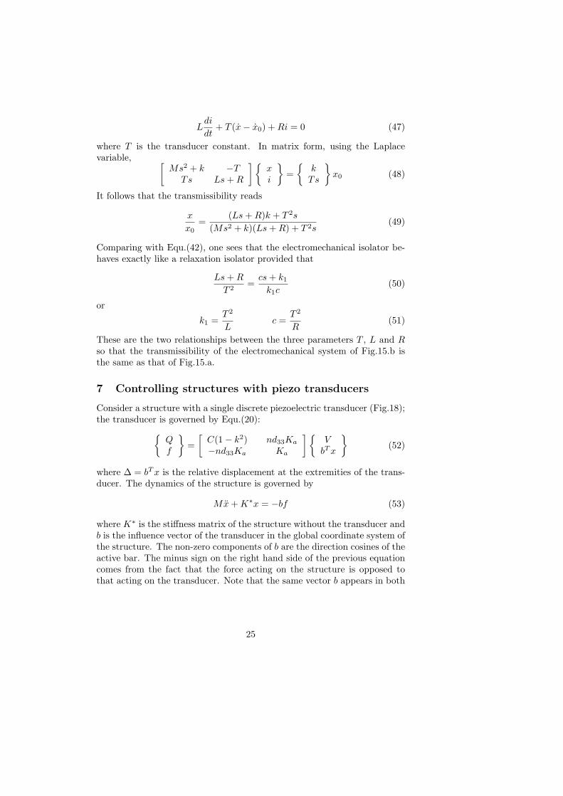
Figure 22. Root locus plot for inductive shunting (only the upper half isshown). The optimum damping at Q is achieved for αe = 1 and ξe = Ki;the maximum modal damping is ξi ≃ Ki/2.

For various values of ωi/Ωi (or Ki), the optimum poles at Q move alonga circle of radius Ωi (Fig.22.d). The corresponding damping ratio can beobtained easily by identifying the previous equation with the classical formof the damped oscillator, s2 + 2ξiΩis+Ω2

i = 0, leading to

ξi =1

2(Ω2

i

ω2i

− 1)1/2 =Ki

2=

1

2(k2νi1− k2

)1/2 (87)

This value is significantly higher than that achieved with purely resistiveshunting [it is exactly the square-root of (75)]. Note, however, that it ismuch more sensitive to the tuning of the electrical parameters on the tar-

34

0.1 1 10

0

0.2 0.5 2 5

!0i=!iFrequency ratio

Resistive

shunting0.05

0.1

0.15

0.2

0.25

0.3

Inductive

shunting

øi

p2 p1

Figure 23. Evolution of the damping ratio of the inductive and resistiveshunting with the de-tuning of the structural mode. ωi is the naturalfrequency for which the shunt has been optimized, ω′

i is the actual value(k = 0.5, νi = 0.3).

geted modes. This is illustrated in Fig.23, which displays the evolutionof the damping ratio ξi when the actual natural frequency ω′

i moves awayfrom the nominal frequency ωi for which the shunt has been optimized (thedamping ratio associated with p1 and p2 is plotted in dotted lines; the ratioω′i/Ω

′i is kept constant in all cases). One sees that the performance of the

inductive shunting drops rapidly below that of the resistive shunting whenthe de-tuning increases. Note that, for low frequency modes, the optimuminductance value can be very large; such large inductors can be synthesizedelectronically. The multimodal passive damping via resonant shunt has beeninvestigated by [Hollkamp, 1994].

Bibliography

CADY, W.G., Piezoelectricity: an Introduction to the Theory and Applica-tions of Electromechanical Phenomena in Crystals, , McGrawHill, 1946.

CRANDALL, S.H., KARNOPP, D.C., KURTZ, E.F, Jr., PRIDMORE-BROWN, D.C. Dynamics of Mechanical and Electromechanical Systems,McGraw-Hill, N-Y, 1968.

DE BOER, E., Theory of Motional Feedback, IRE Transactions on Audio,

35

15-21, Jan.-Feb., 1961.HOLTERMAN, J. & GROEN, P. An Introduction to Piezoelectric Materials

and Components, Stichting Applied Piezo, 2012.HOLLKAMP, J.J. Multimodal passive vibration suppression with piezoelec-

tric materials and resonant shunts, J. Intell. Material Syst. Structures,Vol.5, Jan. 1994.

HUNT, F.V. Electroacoustics: The Analysis of Transduction, and its His-torical Background, Harvard Monographs in Applied Science, No 5, 1954.Reprinted, Acoustical Society of America, 1982.

IEEE Standard on Piezoelectricity. (ANSI/IEEE Std 176-1987).VAN RANDERAAT, J. & SETTERINGTON, R.E. (Edts) Philips Appli-

cation Book on Piezoelectric Ceramics, Mullard Limited, London, 1974.Physik Intrumente catalogue, Products for Micropositioning (PI GmbH).PRATT, J., FLATAU, A. Development and analysis of self-sensing magne-

tostrictive actuator design, SPIE Smart Materials and Structures Con-ference, Vol.1917, 1993.

PREUMONT, A. Vibration Control of Active Structures, An Introduction,Third Edition, Springer, 2011.

PREUMONT, A. Mechatronics, Dynamics of Electromechanical and Piezo-electric Systems, Springer, 2006.

ROSEN, C.A. Ceramic transformers and filters, Proc. Electronic Compo-nent Symposium, p.205-211, 1956.

UCHINO, K. Ferroelectric Devices, Marcel Dekker, 2000.WOODSON, H.H., MELCHER, J.R. Electromechanical Dynamics, Part I:

Discrete Systems, Wiley, 1968.

36