Electrochemical Time of Flight for Rapid and Direct

University of Arkansas, FayettevilleScholarWorks@UARK

Theses and Dissertations

5-2017

Electrochemical Time of Flight for Rapid andDirect Measurement of Diffusion CoefficientsJonathan C. MoldenhauerUniversity of Arkansas, Fayetteville

Follow this and additional works at: http://scholarworks.uark.edu/etd

Part of the Analytical Chemistry Commons, and the Physical Chemistry Commons

This Dissertation is brought to you for free and open access by ScholarWorks@UARK. It has been accepted for inclusion in Theses and Dissertations byan authorized administrator of ScholarWorks@UARK. For more information, please contact [email protected], [email protected].

Recommended CitationMoldenhauer, Jonathan C., "Electrochemical Time of Flight for Rapid and Direct Measurement of Diffusion Coefficients" (2017).Theses and Dissertations. 1951.http://scholarworks.uark.edu/etd/1951

http://scholarworks.uark.edu?utm_source=scholarworks.uark.edu%2Fetd%2F1951&utm_medium=PDF&utm_campaign=PDFCoverPages

http://scholarworks.uark.edu/etd?utm_source=scholarworks.uark.edu%2Fetd%2F1951&utm_medium=PDF&utm_campaign=PDFCoverPages

http://scholarworks.uark.edu/etd?utm_source=scholarworks.uark.edu%2Fetd%2F1951&utm_medium=PDF&utm_campaign=PDFCoverPages

http://network.bepress.com/hgg/discipline/132?utm_source=scholarworks.uark.edu%2Fetd%2F1951&utm_medium=PDF&utm_campaign=PDFCoverPages

http://network.bepress.com/hgg/discipline/139?utm_source=scholarworks.uark.edu%2Fetd%2F1951&utm_medium=PDF&utm_campaign=PDFCoverPages

http://scholarworks.uark.edu/etd/1951?utm_source=scholarworks.uark.edu%2Fetd%2F1951&utm_medium=PDF&utm_campaign=PDFCoverPages

mailto:[email protected],%[email protected]

Electrochemical Time of Flight for Rapid and Direct Measurement of Diffusion Coefficients

A dissertation submitted in fulfillment of the requirements for the degree of

Doctor of Philosophy in Chemistry

by

Jonathan Moldenhauer

Valparaiso University

Bachelor of Science in Chemistry, 2012

May 2017

University of Arkansas

This dissertation is approved for recommendation to the Graduate Council.

Dr. David Paul

Dissertation Director

Dr. Bill Durham Dr. Ingrid Fritsch

Committee Member Committee Member

Dr. Julie Stenken

Committee Member

Abstract

The determination of diffusion coefficients is of fundamental importance to the understanding of

electrochemistry and sensors. Developing a method by which diffusion coefficients of Red/ox active

analytes can be determined quickly and elegantly, would be a great advancement over presently

accepted methods. This dissertation reports the reviving electrochemical time of flight (ETOF), and

developing a method that allows for empirical determination of diffusion coefficients from a single

measurement. ETOF is a generate and detect experiment where the time an electrochemically generated

species takes to transit a known distance is measured and related to the diffusion coefficient of the

species. The determined diffusion coefficient of ferricyanide, 7.3(±0.7) x 10-6

cm2/s, was within the 95%

confidence interval of the literature value, using the traditional ETOF data treatment. In this dissertation a

new treatment of the data, the Moldenhauer treatment, where a diffusional calibration curve is

constructed using multiple species of known diffusion coefficient and measuring their transit times at a set

distance. The calibration curve constructed in aqueous solutions found the diffusion coefficient of

ruthenium(II) hexamine to be within the 95% confidence interval of what has been reported in the

literature. The same calibration was also used to determine diffusion coefficients of aqueous probe

molecules in a more viscous solution of 20% v/v ethylene glycol and water. Computational modeling was

used to further optimize generator pulse widths to allow for a greater linear range of determineable

diffusion coefficients. It was shown that an empirically determined aqueous calibration can be used to

determine diffusion coefficients in organic solvents. The diffusion coefficient of ferrocene was determined

to be 2.4(±0.1) x10-5

cm2/s after modeling directed optimum generator pulse widths. In addition diffusion

coefficients were determined for tetrabutylammonium dioxovanadium(V) dipicolinate (3.9(±0.2) x 10─6

cm2/s), and ruthenium (II) bisbipyridine dichloride (9.3(±0.4)x10

─6 cm

2/s), which do not have published

diffusion coefficients presently. Int the future, this same method could be used to determine diffusion

coefficients in membranes and complex solvents such as ionic liquids.

Acknowledgements

Special thanks to all the support staff in the Chemistry and Biochemistry department for all the

help they provide graduate students during their time here.

Also, a special thanks to my committee and my lab mates and my other colleagues and friends in

the Department of Chemistry and Biochemistry at the University of Arkansas, for all of the support and

help you have provided me during my time here.

I would also like to specifically acknowledge the grammatical and formatting help that was

provided me by my personal editor, Cassandra Gronendyke, who has read all of my papers before

submission.

And finally thanks to the Thesis and Dissertation Group at CAPS (Counseling and Psychological

Services) at Pat Walker Health Center. Your emotional support during this tough phase of my life has

been really valuable and important to me.

Dedication

I would like to dedicate this dissertation to several people. Firstly, my significant other Cassandra

Gronenedyke, for having had to deal with me when research is going well and when research was going

poorly. Secondly, to my laid back boss, Dr. David Paul, and his catchphrase “Dumb looks are Free”. And

finally to my parents who at least only minimally asked any of those questions that grad-students dread

hearing.

Table of Contents

Introduction.................................................................................................................................................... 1

A Comparison of Methods for determining diffusion coefficients .............................................................. 2

Summary of Presented Work .................................................................................................................... 6

References ................................................................................................................................................ 8

Rapid and Direct Determination of Diffusion Coefficients Using Microelectrode Arrays ............................ 11

Abstract ................................................................................................................................................... 12

Introduction.............................................................................................................................................. 13

Experimental ........................................................................................................................................... 18

Generator Controller and LabView Software: ..................................................................................... 18

Working Electrode Array: .................................................................................................................... 20

Chemicals: ........................................................................................................................................... 20

Experimental Parameters: ................................................................................................................... 20

Results and Discussion ........................................................................................................................... 22

Applied potentials: ............................................................................................................................... 22

ETOF Data Analysis: ........................................................................................................................... 23

Functionality of Hardware and Software: ............................................................................................ 25

Proving K a Constant for Multiple Red/OX Species: ........................................................................... 26

Determination of Diffusion Coefficients in Viscous Solutions: ............................................................ 29

Conclusions ............................................................................................................................................. 31

Acknowledgements ................................................................................................................................. 32

References .............................................................................................................................................. 32

Optimization of Electrochemical Time of Flight Measurements for Precise Measurements of Diffusion

Coefficients over a Wide Range in Various Media ..................................................................................... 35

Abstract ................................................................................................................................................... 36

Introduction.............................................................................................................................................. 37

Theoretical optimization of precision and accuracy in ETOF measurements ......................................... 39

Experimental ........................................................................................................................................... 44

Hardware ............................................................................................................................................. 44

Chemicals ............................................................................................................................................ 44

Conditions of electrochemical measurements .................................................................................... 45

Results and Discussion ........................................................................................................................... 47

Aqueous Diffusion Coefficient Calibration Curves Can Extend to Organic Solvents .......................... 48

Application to VO(acac)2 in acetonitrile / 0.1 M TBAPF6 ..................................................................... 50

Conclusions ............................................................................................................................................. 52

Acknowledgements ................................................................................................................................. 53

Future Prospects and Conclusions ............................................................................................................. 56

Recalibration of Oxygen Sensing Electrodes.......................................................................................... 56

A Brief Comparison of ETOF to Other Methods for determination of Diffusion through membranes ..... 57

Conclusion............................................................................................................................................... 61

References .................................................................................................................................................. 61

Appendix 1: Detailed Device Construction .................................................................................................. 63

Introduction to Labview: .......................................................................................................................... 63

Initial Development of Program and Device Design ............................................................................... 66

Improved Program and Device Design: .................................................................................................. 67

References .............................................................................................................................................. 71

Table of Figures

Figure 1 ....................................................................................................................................................... 15

Figure 2 ....................................................................................................................................................... 16

Figure 3 ....................................................................................................................................................... 18

Figure 4 ....................................................................................................................................................... 19

Figure 5 ....................................................................................................................................................... 21

Figure 6 ....................................................................................................................................................... 24

Figure 7 ....................................................................................................................................................... 26

Figure 8 ....................................................................................................................................................... 28

Figure 9: ...................................................................................................................................................... 30

Figure 10 ..................................................................................................................................................... 42

Figure 11 ..................................................................................................................................................... 42

Figure 12 ..................................................................................................................................................... 47

Figure 13 ..................................................................................................................................................... 49

Figure 14 ..................................................................................................................................................... 59

Figure 15 ..................................................................................................................................................... 65

Figure 16: .................................................................................................................................................... 66

Figure 17 ..................................................................................................................................................... 68

Figure 18 ..................................................................................................................................................... 69

Figure 19 ..................................................................................................................................................... 70

List of Published Papers

Chapter 1: " Rapid and Direct Determination of Diffusion Coefficients Using Microelectrode Arrays "

Moldenhauer, Jonathan. J. Electrochem. Soc. . v. 163 no. 8. 2016. p. H672 - H678. Published

1

Introduction

Diffusion is both an important property to electrochemistry and a property commonly determined using

electrochemistry. Diffusion of molecules through a solvent is important to measure when trying to

elucidate electrochemical mechanisms (1-9) for, design of better batteries and other energy

applications(10-22), electrochemical sensors(23-29), optimization of industrial processes(30), and for

calculating conductive properties of electrolytes and solutions (31-43). All of these processes have steps

that are limited by the mass transport of chemical species, from the most fundamental research in

electrochemical measurements to more applied areas of research such as energy storage and

conversion or medical sensors(44) the values of diffusion coefficients are of great importance . Diffusion

coefficients are everywhere because mass transport is everywhere and measuring them would add to our

understanding of the world around us.

In order to better understand the importance of research into methods of determining diffusion

coefficients, it is best to discuss an application for which diffusion coefficients need to be measured, that

area being a growing area of electrochemistry: room temperature ionic liquids (RTILs). These liquid

organic molecules are solvents that also serve as a supporting electrolyte for electrochemical

experiments. RTILs have an advantage over other liquid salts in that they can be studied in a lab setting

without special high-temperature equipment. However, RTILs are an area of great interest in

electrochemistry right now, and because of their solvation properties and wide potential windows, they

provide a new area for electrochemical study, and few diffusion coefficients for molecules in RTIL’s have

been published. Diffusional properties of species in these solvents is important for determining how well

they can be used for electrocatalyzed synthesis(40), such as electrocatalyzed carboxylation(3), and as a

solvent for other types of electrochemical measurements for physical chemistry and mechanistic

studies(8, 41, 42). RTILs can serve as the best options for electrolyte solutions in batteries(20) where

output currents are limited by diffusion between the anode and the cathode(38). Faster diffusion

translates to less impedance to current across the separator(12). Measuring diffusion coefficients in other

solvents such as high temperature ionic liquids that could be used in large storage batteries for power

plants and bulk power generation(4, 31, 45), as well as for their use in fuel cells would also be

important(14). Knowledge of diffusion coefficients in RTILs also contributes to the understanding of

2

mechanisms behind various photocells such as dye-sensitized solar cells(19, 43). Ionic liquids also have

very large and adjustable potential windows and that leads them to be exciting as new solvents for

electrochemical systems(36). Diffusion coefficients shift based on the purity of ionic liquids(37), for

instance the water content in the ionic liquid(39), so the possibility of determining purity via diffusion

coefficients exists.

For all of these reasons there needs to be a way to quickly and easily determine diffusion coefficients.

Electrochemical Time of Flight in the literature appears to be a quick and effective method of determining

diffusion coefficients. However, no one, yet, has used ETOF for anything more than a method to provide

empirical backing for computational diffusion models. This dissertation shows that ETOF can be used for

the determination of diffusion coefficients of Red/Ox species and diffusion coefficients in unlike solvents.

This broadens the applicability of a method that has been mostly ignored since its inception. ETOF can

be used to determine diffusion coefficients with a simple measurement and in less time than traditional

methods. If broad application could be shown, as it has in this dissertation, researchers would be able to

use it as a common method for determination of diffusion coefficients.

A Comparison of Methods for determining diffusion coefficients

One of the most common ways to evaluate the diffusion of Red/Ox active molecules in a bulk solution is

to use rotating disk electrodes (RDE) and the Levich equation, Equation 1 relating the diffusion of a

species to its limiting current(46).

Equation 1

Where the limiting current, ilev, is proportional to ;n the number of electrons transferred, F Faraday’s

constant, D the diffusion coefficient, v the kinematic viscosity of the supporting electrolyte, w the rotation

rate, and Cs the analyte concentration in bulk(47). This method requires one to have prior knowledge of

the concentration of the analyte in question, the electrode area, and the number of electrons transferred,

the viscosity of the system, and electron transfer kinetics. So this method works well only for fully

elucidated systems such as any number of common probe molecules, i.e. ferricyanide, ferrocyanide, etc..

There are several limitations to determining the diffusion coefficient of an analyte using the Levich

3

equation. There is an issue with very viscous solvents such as some ionic liquids where RDE techniques

fail because true diffusion controlled limiting currents are difficult to achieve (48). However the Levich

Equation is still the standard method in conventional solvents, even though that concentration is the only

known and controlled factor (49). Sometimes the number of electrons transferred is an unknown quantity,

so an alternative method to determining diffusion coefficients is needed, One such alternative is ETOF,

which is the only technique capable of determining diffusion coefficients without foreknowledge of the

concentration of the analyte, the electroactive area, the number of electrons transferred, or the viscosity

of the solvent(50), and in small volumes.

Royce Murray and his group were the first to use the ETOF experiment in the late 1980s(51). They were

interested in the apparent diffusion of electrons across conducting polymers. They sandwiched a

conducting polymer between two electrodes and monitored a pulse of charge as it travelled between

them. This they related to the Einstein equation, Equation 2, where d is the distance traveled (space

between the electrodes), θ is a numerical constant that is related to the geometry of the electrodes, De is

the diffusion coefficient of an electron through the polymer, and tmax is the time at which there was a

maximum current at the detecting electrode.

Equation 2

ETOF then was applied to determining of the diffusion coefficient of an analyte in bulk solution. In 1990

Stuart Licht(52) published a paper which laid out a method for using individually addressable

microelectrode array and ETOF to determine the diffusion coefficient of a molecule without first knowing

its concentration, simply by knowing the distance and the time that the electrochemically active species

took travel between the generator and the detector electrode. From his work he determined that the

diffusion coefficient (D) was inversely proportional to the time of maximum collection and that the time of

maximum collection (tmax) was directly proportional to the distance (d) squared as related by an

empirically determined proportionality constant, Equation 3 (52).

Equation 3

4

It is important to note that the time of maximum collection is measured from the middle of the generation

pulse to the peak on the collector current. The distance, d, is measured from the center of the generator

electrode to the edge of the collection electrode. He also modeled this equation using a random walk

simulation and arrived at an equation that appears to be in close agreement with the above,

, which he stated had an experimental uncertainty of 10%(52).

Christian Amatore(50) continued to look at the above method as a way of determining diffusion

coefficients of analyte molecules in a bulk solution explaining why pulsed generation is better than

continuous generation. This is because it is easier to determine the time of maximum collection current

than the time as which a steady state current is achieved. In addition, when the generator is polarized for

longer periods of time there is a greater chance of molecules from the detector diffusing back to the

generator(50). This diffusion from the collector back to the generator (sometimes called diffusion layer

over-lap or cross-talk) lengthens the amount of time it takes to achieve the limiting current, and

determining the tmax is difficult. Longer times also require very stable redox species to serve as the

analyte(50). Amatore also reconstructed Licht’s equation, Equation 4, where d is still the distance, K is the

geometry constant for the electrode system that must be determined empirically for each electrode

system, D is the diffusion coefficient of the detected species, and tmax is the time of maximum

collection(50).

√ Equation 4

Amatore correctly determined the diffusion coefficients for the ferri-ferrocyanide system in bulk solution by

ETOF using the above equation after finding K for the electrode array.

Despite there being some skepticism about generate and detect experiments working in low electrolyte

concentrations(53), with slight experimental modifications, electrochemical time of flight can determine a

variety of other interfacial parameters. Using galvanic generation, Slowinska was able to determine the

capacitance of solid films on potentiometric sensors. The sensing method at the detector is

potentiometric, the method being called potentiometric electrochemical time of flight or P-ETOF(54-56).

The same group that did the P-ETOF experiments also applied electrochemical time of flight to viscous

5

solutions and showed the ability to determine diffusion coefficients of analyte molecules as they change

with increasing solution viscosity(57). Others have used it for the determination of diffusion coefficients in

glucose solutions and gels(58) and still another group has shown that ETOF can actually be used for the

determination of the diffusion coefficient through a solid substrate(59).

However there are other methods of determining diffusion coefficients that include both electrochemical

and non-electrochemical means. Other electrochemical means of determining diffusion coefficients

include, chronoamperometry (25, 35) and scanning electrochemical microscopy (SECM)(34). The Cottrell

equation (Equation 5) relates current, I(t), to the time, t, and concentration of the analyte, Co, in solution.

( )

Equation 5

Unfortunately, it has many of the same limitations as the Levich equation, requiring knowledge of the

electroactive area of the electrode, A, and the number of electrons transferred, n. The equation can be

used in both voltammetric and amperometric experiments but more commonly amperometric

measurements of diffusion coefficients are performed.

Another method similar to ETOF that can be used to determine diffusion coefficients is scanning

electrochemical microscopy (SECM). This uses an ultramicroelectrode (UME) electrode held a short

distance vertically from a surface, or substrate, and the UME, or tip, are used as a detector and a

generator electrode respectively and biased so that opposing reactions are happening at each

electrode(60-65). SECM is typically used for surface studies of electrode arrays and thin films, both

making use of the fact that the tip can be moved and determine spatial data about the resistive or

conductive nature of the substrate. It can also be used for kinetics studies and the determination of

diffusion coefficients(60, 62, 65). Determining the diffusion coefficient ratio of the couple in the solution

from the limiting currents at the detector and from the feedback to the generator is based on knowing the

current at time equals infinity, the electroactive area of the electrode, and the starting concentration of

one the analytes (61). This experiment returns to a methodology that requires knowledge of the

electroactive area of the electrode and the initial concentration of one of the species, however it does not

require knowledge of how far electrodes are separated.

6

There are still other non-electrochemical options, such as pulsed field gradient NMR, which one can use

to determine the diffusion coefficient of a species. In these experiments diffusion of the ions such as

lithium, that are detectible by NMR, is measured by the decay of echo intensity precession of the nuclei

on the atoms to the RF excitation(12). This method is commonly used for lithium ions to examine gel

electrolytes or other materials for use in batteries(11-13). This makes it a popular method for using with

viscous organic solvents like the ionic liquids previously mentioned that are liquid organic anions and

cations, because they are common for use as solvents in batteries and because of their viscosity it

becomes difficult to use for hydrodynamic experiments(11). This method is also primarily used to

determine the ionic conductivities of organic solvents because it is easy to measure the diffusion

coefficient of atomic ions(32). This method can also be used for organic molecules diffusing in ionic

liquids(33), the solubility and diffusion of gas molecules such as CO2 in ionic liquids(30), and organic

molecules that are not electrochemically active(66).

The power of ETOF is that as opposed to hydrodynamic methods it can be used over a wide range of

viscosities and use much smaller volumes. Meaning that the Moldenhauer treatment, constructing

diffusional calibration curves, could be used for determination of diffusion coefficients in highly viscous

ionic liquids, but unfortunately a limited amount of information on diffusion coefficients for probe

molecules in ionic liquids and liquids of increased viscosity exists. Such a calibration curve could not be

constructed without knowledge of diffusion coefficients in the specific solvent system used. What was

revealed in this study was that it is possible to construct a diffusional calibration curve in one solvent

system using a species of known diffusion coefficients; then use that same calibration curve to determine

the diffusion coefficients of molecules in different solvent systems by simply measuring the TOF and

using the calibration curve to determine the diffusion coefficient. This is something that has never been

shown in by showing that ETOF can be applied to numerous unlike compounds in unlike solvents using

an aqueous calibration curve, a stepping stone for research in other solvent systems.

Summary of Presented Work

ETOF methods as we present it here has never before been used before to determine diffusion

coefficients of multiple unlike species. In fact while it has been used empirically in the past it has never

7

been previously utilized beyond finding a diffusion coefficient of a single molecule or to verify diffusional

models of electrochemical experiments. The work here provides the groundwork needed so that one

could use this as a primary technique for the determination of diffusion coefficients, and especially to

apply this technique to the diffusion of molecules through membranes and for the determination of

diffusion coefficients through ionic liquids. Although these applications are important, only diffusion

coefficient in bulk solution were determined here.

The first paper of this volume shows that one can make an empirical calibration curve by rearranging the

ETOF equation and describes the construction of the Generation Electrode Controller (GEC) that was

used to control the voltage pulse on the generation electrode. The GEC is controlled by a National

Instrument’s LabVIEW program providing for pulsed generation on the second working electrode of a CHI

750series potentiostat, more details on the construction of the device can be found in appendix 1. We

were then able to determine diffusion coefficients using an empirical calibration of a microelectrode array

using both the traditional treatment of ETOF using as single analyte and our non-traditional data

treatment using a series of standards to construct a calibration curve for the determination of diffusion

coefficients based on their time of flight. The curves in this paper suggested that there was an intercept

that we later determined was unimportant.

In the second paper we approached the question of: What is the range of diffusion coefficients that can

be determined by using our alternative data treatment (with any accuracy)? For that we collaborated with

Christian Amatore and Catherine Sella to model our experiment to optimize the parameters over a wide

range. Here we report for the first time that K, is dependent on the pulse width at the generator as well as

the gap between the generator and the collector. K is constant only for a range of generation pulse

widths and that as long as the generation pulse is tuned correctly, one can determine diffusion

coefficients for a wide range of analytes across at least 1 order of magnitude using a single electrode

geometry. This paper also shows that diffusion coefficients can be determined using the Moldenhauer

data treatment in vastly different solvent systems and viscosities of solutions, which was something that

had not previously been reported in the literature.

8

References

1. L. E. Barrosse-Antle, C. Hardacre and R. G. Compton, J Phys Chem B, 113, 2805 (2009).

2. R. G. Evans, O. V. Klymenko, P. D. Price, S. G. Davies, C. Hardacre and R. G. Compton, Chemphyschem, 6, 526 (2005). 3. Y. Hiejima, M. Hayashi, A. Uda, S. Oya, H. Kondo, H. Senboku and K. Takahashi, Phys Chem Chem Phys, 12, 1953 (2010). 4. H. Yabe, S. Hikino, K. Ema and Y. Ito, Electrochim. Acta, 35, 1233 (1990).

5. J. Ma, M. Yan, A. M. Kuznetsov, A. N. Masliy, G. Ji and G. V. Korshin, Environ. Sci. Technol., 49, 13542 (2015). 6. S. N. Nacer and T. Lanez, Res. Rev.: J. Chem., 2, 28 (2013).

7. Y. Nishiyama, M. Terazima and Y. Kimura, J. Phys. Chem. B, 113, 5188 (2009).

8. M. J. A. Shiddiky, A. A. J. Torriero, C. Zhao, I. Burgar, G. Kennedy and A. M. Bond, J Am Chem Soc, 131, 7976 (2009). 9. S. J. Woltman, M. R. Alward and S. G. Weber, Anal. Chem., 67, 541 (1995).

10. D. R. Baker, C. Li and M. W. Verbrugge, J. Electrochem. Soc., 160, A1794 (2013).

11. P. M. Bayley, G. H. Lane, N. M. Rocher, B. R. Clare, A. S. Best, D. R. MacFarlane and M. Forsyth, Phys Chem Chem Phys, 11, 7202 (2009). 12. S. Indris, R. Heinzmann, M. Schulz and A. Hofmann, J. Electrochem. Soc., 161, A2036 (2014).

13. Z.-Y. Mao, Y.-P. Sun and K. Scott, J. Electroanal. Chem., 766, 107 (2016).

14. M. Haibara, S. Hashizume, H. Munakata and K. Kanamura, Electrochim. Acta, 132, 208 (2014).

15. A. K. Sethurajan, S. A. Krachkovskiy, I. C. Halalay, G. R. Goward and B. Protas, J. Phys. Chem. B, 119, 12238 (2015). 16. A. Shvarev and E. Bakker, Anal Chem, 77, 5221 (2005).

17. N. Spinner and W. E. Mustain, J. Electroanal. Chem., 711, 8 (2013).

18. E. Talaie, P. Bonnick, X. Sun, Q. Pang, X. Liang and L. F. Nazar, Chem. Mater., 29, 90 (2017).

19. P. Wachter, M. Zistler, C. Schreiner, M. Berginc, U. O. Krasovec, D. Gerhard, P. Wasserscheid, A. Hinsch and H. J. Gores, J. Photochem. Photobiol., A, 197, 25 (2008). 20. R. Wibowo, J. S. E. Ward and R. G. Compton, J Phys Chem B, 113, 12293 (2009).

21. D.-Y. Yoo, I.-H. Yeo, W. I. Cho, Y. Kang and S.-i. Mho, Anal. Sci., 29, 1083 (2013).

22. S. Zhang, X. Li and D. Chu, Electrochim. Acta, 190, 737 (2016).

23. R. Devasenathipathy, V. Mani and S.-M. Chen, Talanta, 124, 43 (2014).

9

24. M. Elyasi, M. A. Khalilzadeh and H. Karimi-Maleh, Food Chem, 141, 4311 (2013).

25. H. Heli, M. Hajjizadeh, A. Jabbari and A. A. Moosavi-Movahedi, Anal. Biochem., 388, 81 (2009).

26. H. Li, Z. Xu, L.-N. Ji and W.-S. Li, J. Appl. Electrochem., 35, 235 (2005).

27. M. Mazloum-Ardakani, H. Beitollahi, M. K. Amini, F. Mirkhalaf and B.-F. Mirjalili, Biosens Bioelectron, 26, 2102 (2011). 28. M. Tabeshnia, M. Rashvandavei, R. Amini and F. Pashaee, J. Electroanal. Chem., 647, 181 (2010). 29. X. Ye, Y. Du, D. Lu and C. Wang, Anal Chim Acta, 779, 22 (2013).

30. K. Kortenbruck, B. Pohrer, E. Schluecker, F. Friedel and I. Ivanovic-Burmazovic, J. Chem. Thermodyn., 47, 76 (2012). 31. R. Brookes, A. Davies, G. Ketwaroo and P. A. Madden, J Phys Chem B, 109, 6485 (2005).

32. L. Garrido, A. Mejia, N. Garcia, P. Tiemblo and J. Guzman, J Phys Chem B, 119, 3097 (2015).

33. A. Kaintz, G. Baker, A. Benesi and M. Maroncelli, J Phys Chem B, 117, 11697 (2013).

34. F. O. Laforge, T. Kakiuchi, F. Shigematsu and M. V. Mirkin, J Am Chem Soc, 126, 15380 (2004).

35. K. R. J. Lovelock, A. Ejigu, S. F. Loh, S. Men, P. Licence and D. A. Walsh, Phys Chem Chem Phys, 13, 10155 (2011). 36. S. Chanfreau, B. Yu, L.-N. He and O. Boutin, J. Supercrit. Fluids, 56, 130 (2011).

37. S. Eisele, M. Schwarz, B. Speiser and C. Tittel, Electrochim. Acta, 51, 5304 (2006).

38. V. L. Martins, N. Sanchez-Ramirez, M. C. C. Ribeiro and R. M. Torresi, Phys Chem Chem Phys, 17, 23041 (2015). 39. A. Menjoge, J. Dixon, J. F. Brennecke, E. J. Maginn and S. Vasenkov, J Phys Chem B, 113, 6353 (2009). 40. L. Nagy, G. Gyetvai, L. Kollar and G. Nagy, J Biochem Biophys Methods, 69, 121 (2006).

41. A. W. Taylor, P. Licence and A. P. Abbott, Phys Chem Chem Phys, 13, 10147 (2011).

42. M. A. Vorotyntsev, V. A. Zinovyeva, D. V. Konev, M. Picquet, L. Gaillon and C. Rizzi, J Phys Chem B, 113, 1085 (2009). 43. M. Zistler, P. Wachter, P. Wasserscheid, D. Gerhard, A. Hinsch, R. Sastrawan and H. J. Gores, Electrochim. Acta, 52, 161 (2006). 44. A. J. Bard and L. R. Faulkner, Electrochemical Methods: Fundamentals and Applications, p. 833, John Wiley & Sons Inc., Hoboken, NJ (2001). 45. H. Yabe, K. Ema and Y. Ito, Electrochim. Acta, 34, 1479 (1989).

46. D. A. Gough and J. K. Leypoldt, Anal. Chem., 51, 439 (1979).

47. T. H. Silva, S. V. P. Barreira, C. Moura and F. Silva, Port. Electrochim. Acta, 21, 281 (2003).

10

48. C. L. Bentley, A. M. Bond, A. F. Hollenkamp, P. J. Mahon and J. Zhang, Anal Chem, 85, 2239 (2013). 49. M. Chatenet, M. B. Molina-Concha, N. El-Kissi, G. Parrour and J. P. Diard, Electrochim. Acta, 54, 4426 (2009). 50. C. Amatore, C. Sella and L. Thouin, J. Electroanal. Chem., 593, 194 (2006).

51. B. J. Feldman, S. W. Feldberg and R. W. Murray, J. Phys. Chem., 91, 6558 (1987).

52. S. Licht, V. Cammarata and M. S. Wrighton, J. Phys. Chem., 94, 6133 (1990).

53. W. Hyk, A. Nowicka and Z. Stojek, Anal. Chem., 74, 149 (2002).

54. H. A. Elsen, K. Slowinska, E. Hull and M. Majda, Anal. Chem., 78, 6356 (2006).

55. K. Slowinska, S. W. Feldberg and M. Majda, J. Electroanal. Chem., 554-555, 61 (2003).

56. K. Slowinska and M. Majda, J. Solid State Electrochem., 8, 763 (2004).

57. D. Ky, C. K. Liu, C. Marumoto, L. Castaneda and K. Slowinska, J. Controlled Release, 112, 214 (2006). 58. A. Varga, G. Gyetvai, L. Nagy and G. Nagy, Anal. Bioanal. Chem., 394, 1955 (2009).

59. V. Cammarata, D. R. Talham, R. M. Crooks and M. S. Wrighton, J. Phys. Chem., 94, 2680 (1990). 60. R. D. Martin and P. R. Unwin, J. Electroanal. Chem., 439, 123 (1997).

61. R. D. Martin and P. R. Unwin, J. Chem. Soc., Faraday Trans., 94, 753 (1998).

62. R. D. Martin and P. R. Unwin, Anal. Chem., 70, 276 (1998).

63. C. G. Zoski, C. R. Luman, J. L. Fernandez and A. J. Bard, Anal. Chem. (Washington, DC, U. S.), 79, 4957 (2007). 64. C. G. Zoski, B. Liu and A. J. Bard, Anal. Chem., 76, 3646 (2004).

65. C. G. Zoski, J. C. Aguilar and A. J. Bard, Anal. Chem., 75, 2959 (2003).

66. O. Mayzel, O. Aleksiuk, F. Grynszpan, S. E. Biali and Y. Cohen, J. Chem. Soc., Chem. Commun.,

1183 (1995).

11

Rapid and Direct Determination of Diffusion Coefficients Using Microelectrode Arrays

Jonathan Moldenhauer, Madeline Meier, and David W. Paul

Department of Chemistry and Biochemistry


1 University of Arkansas

Fayetteville, AR 72701

USA

This is an open access article distributed under the terms of the Creative Commons Attribution 4.0

License (CC BY, http://creativecommons.org/licenses/by/4.0/), which permits unrestricted reuse of the

work in any medium, provided the original work is properly cited.

12

Abstract: The sensitivity of amperometric sensors is typically set by the rate diffusion of the analyte to

the electrode surface, so determining diffusion coefficients in various electrolyte solutions is of

fundamental interest. It has been theoretically shown and verified that diffusion coefficients of

electrochemically generated analytes can be determined using electrochemical time of flight (ETOF), a

method that uses an electrochemical array in which one electrode generates a Red/Ox species, and

measures the analyte diffusion times to collecting electrodes of differing distances from a stationary

generator. ETOF has the potential to greatly simplify the determination of diffusion coefficients as the

analyte concentration, the electroactive area, the solution viscosity, and the electron transfer kinetics can

remain unknown. Here we demonstrate a rearrangement of the ETOF experiment in which the

electrochemical flight time is measured for a series of different Red/Ox species of known diffusion

coefficients at single distance. We show this a valid application of a method that has existed for almost 30

years, by determining diffusion coefficients for ruthenium (II) hexamine, and diffusion coefficients in

solutions of increased viscosity.

13

Introduction

Diffusion coefficients are important because they set the sensitivity of amperometric sensors and they are

a fundamental property both in membrane permeability and in electrochemical measurements. The most

common method of determining diffusion coefficients for analytes in bulk solutions or through gels and

membranes relies on the rotating disk electrode (RDEs) (1-7) or the rotating ring disk electrode (RRDE)

(8). This method determines the diffusion coefficients, D, from the slope of a Levich plot constructed by

measuring limiting currents, IL, as a function of square root of the rotation rate, w, according to the Levich

equation (Equation 1).

Equation 1

Accurate values for the area of the electrode, A, the number of electrons transferred, n, the concentration

of the molecule, C, and the viscosity of the solution, v, must also be known in order to effectively

determine the diffusion coefficient from the slope of a Levich Plot. The diffusion coefficients of molecules

through bulk solution can also be determined quantitatively by wall-jet chronoamperometry(9), or

qualitatively by comparing the CV’s of different compounds because the shape of the CV is related to the

diffusion coefficient of the molecule (10-12). The other primary option for determining diffusion coefficients

of a molecule through a membrane coated over an electrode is impedance spectroscopy (13-18), where

the diffusion of the molecule through a membrane or polymer is related to the impedance of the polymer

or membrane to current flow. As such, the diffusion through the polymer is related directly to the

resistance of charge transfer (mobility) through the membrane, which is related to its conductivity and

directly correlated to the diffusion coefficient by the Nernst-Einstein equation (Equation 2).

Equation 2

Conductance, σ, can be determined from the charge transfer resistance and related to the diffusion

coefficient for the analyte, D, if the concentration, C, the temperature in Kelvin, T, and the charge on the

species, q, are also known, where k is the Boltzmann Constant. The above equation is primarily used

14

when looking at diffusion of ions through solid polymer electrolytes, membranes, and polymer brushes

(13-16).

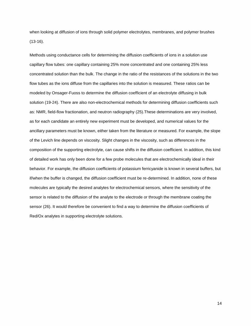
Methods using conductance cells for determining the diffusion coefficients of ions in a solution use

capillary flow tubes: one capillary containing 25% more concentrated and one containing 25% less

concentrated solution than the bulk. The change in the ratio of the resistances of the solutions in the two

flow tubes as the ions diffuse from the capillaries into the solution is measured. These ratios can be

modeled by Onsager-Fuoss to determine the diffusion coefficient of an electrolyte diffusing in bulk

solution (19-24). There are also non-electrochemical methods for determining diffusion coefficients such

as: NMR, field-flow fractionation, and neutron radiography (25).These determinations are very involved,

as for each candidate an entirely new experiment must be developed, and numerical values for the

ancillary parameters must be known, either taken from the literature or measured. For example, the slope

of the Levich line depends on viscosity. Slight changes in the viscosity, such as differences in the

composition of the supporting electrolyte, can cause shifts in the diffusion coefficient. In addition, this kind

of detailed work has only been done for a few probe molecules that are electrochemically ideal in their

behavior. For example, the diffusion coefficients of potassium ferricyanide is known in several buffers, but

if/when the buffer is changed, the diffusion coefficient must be re-determined. In addition, none of these

molecules are typically the desired analytes for electrochemical sensors, where the sensitivity of the

sensor is related to the diffusion of the analyte to the electrode or through the membrane coating the

sensor (26). It would therefore be convenient to find a way to determine the diffusion coefficients of

Red/Ox analytes in supporting electrolyte solutions.

15

In this paper we show that there is an existing method in the literature that has been mostly ignored in the

thirty years since its development. Electrochemical-time-of-flight (ETOF) is a generate-detect experiment

in which an analyte is generated either oxidatively or reductively at one electrode, called the generator; it

is detected by re-reduc ing/re-oxidizing the analyte at a second electrode, called the collector (Figure 1).

Figure 1: The Electrochemical Time of Flight experiment (ETOF). A) Oxidized form (O) in solution and

generator (red) is at open circuit, the collectors (blue) are polarized to an oxidizing potential. B) The

generator is briefly polarized to a reducing potential, converting the O to its reduced form (R). C) R

from the generator has traveled over to the collectors and is reoxidized to O. D) A picture of a

representative electrode array, 25 micron width electrodes, with a 25 micron separation, and 2 mm

long. (Two of the array members on this array have been platinized.)

16

This type of experiment was first reported by Royce Murray, et al., to examine electron diffusion rates

through conducting polymers that were inserted between two fingers on an electrode array(27). The two

electrodes are within micrometers of each other and are often members of a microelectrode array (25, 28-

33).The time it takes the product from the generator to diffuse to the nearest edge of the collector is the

time of flight. If a potential pulse is applied to the generator, a burst of product diffuses to the collector

(Figure 2), and the time of maximum collection, tmc, is measured. The diffusion coefficient in of a Red/Ox

species can then be calculated using Equation 3.

Figure 2: Chronoamperometric transients for the ETOF experiment in ferricyanide: the ferricyanide

reduction current at the generator (red curve and axis) and the ferrocyanide reoxidation current at the

collector (blue curve and axis). The generator electrode is briefly polarized, after this point the

oxidative collector current increases until it reaches a maxima. The time between these two points is

the time of maximum collection.

17

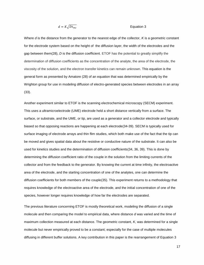
√ Equation 3

Where d is the distance from the generator to the nearest edge of the collector, K is a geometric constant

for the electrode system based on the height of the diffusion layer, the width of the electrodes and the

gap between them(28), D is the diffusion coefficient. ETOF has the potential to greatly simplify the

determination of diffusion coefficients as the concentration of the analyte, the area of the electrode, the

viscosity of the solution, and the electron transfer kinetics can remain unknown. This equation is the

general form as presented by Amatore (28) of an equation that was determined empirically by the

Wrighton group for use in modeling diffusion of electro-generated species between electrodes in an array

(33).

Another experiment similar to ETOF is the scanning electrochemical microscopy (SECM) experiment.

This uses a ultramicroelectrode (UME) electrode held a short distance vertically from a surface. The

surface, or substrate, and the UME, or tip, are used as a generator and a collector electrode and typically

biased so that opposing reactions are happening at each electrode(34-39). SECM is typically used for

surface imaging of electrode arrays and thin flim studies, which both make use of the fact that the tip can

be moved and gives spatial data about the resistive or conductive nature of the substrate. It can also be

used for kinetics studies and the determination of diffusion coefficients(34, 36, 39). This is done by

determining the diffusion coefficient ratio of the couple in the solution from the limiting currents of the

collector and from the feedback to the generator. By knowing the current at time infinity, the electroactive

area of the electrode, and the starting concentration of one of the analytes, one can determine the

diffusion coefficients for both members of the couple(35). This experiment returns to a methodology that

requires knowledge of the electroactive area of the electrode, and the initial concentration of one of the

species, however longer requires knowledge of how far the electrodes are separated.

The previous literature concerning ETOF is mostly theoretical work, modeling the diffusion of a single

molecule and then comparing the model to empirical data, where distance d was varied and the time of

maximum collection measured at each distance. The geometric constant, K, was determined for a single

molecule but never empirically proved to be a constant; especially for the case of multiple molecules

diffusing in different buffer solutions. A key contribution in this paper is the rearrangement of Equation 3

18

Figure 3: The connections between the Generation

Electrode Controller (GEC), the National Instruments cDAQ

modules, and the 750a potentiostat to produce a pulsed

potential waveform at the second working electrode that

would otherwise be impossible with the CHI 750a alone.

into Equation 4, as an alternative data analysis treatment for ETOF data.

√

√ Equation 4

If K is indeed constant, and d is held constant, then by selecting molecules with various and known

diffusion coefficients, it would be possible to construct a curve with slope,

, and with an intercept B,

which is a consequence of the x-intercept which occurs at the fastest diffusion rate able to be

differentiated from tmc= 0 s. This “calibration curve” for the geometry of the array could then be used to

determine the diffusion coefficient for any molecule in any solution. This experiment can be done without

experiencing the loss of signal that occurs when d increases while performing a typical multiple distance

experiment.

Experimental

Generator Controller and LabView Software: Amatore used a multistat (Autolab Pgstat 20 and GPES

software from Ecochemie, Metrohm

Switzerland) to perform these

experiments. There are commercial

instruments with the needed capability

(Bio-Logic, Grenoble, France), but they

are expensive. The bipotentiostats

available in our lab, were not capable of

leaving the second working (generator)

electrode open circuit, nor of providing a

potential pulse. Our solution was to

modify our existing bipotentiostat. The second working electrode from a CHI 750 potentiostat

(CHInsturments, Austin, Texas, USA) was used to provide the potential to the generating electrode. As

with most commercially available bipotentiosats the second working electrode only provides a static

potential that is applied when the experiment initiates.

19

For the application described here, the generator is at open-circuit save for a brief potential pulse. To

accomplish this, a relay was spliced into the second working electrode lead (Figure 3 Generating

Electrode Controller, GEC). Timing and control of the relay was established by LabView software, and a

National Instruments CompactDAQ 9417 controller using a 9403 digital I/O module (National Instruments,

Austin, Texas, USA), attached to a laptop computer (Figure 3). A circuit board was constructed to connect

the relay and control and capture the digital signals between the potentiostat and the digital I/O module.

The GEC went through several iterations before arriving at a final design shown in Figure 4. The D-flip-

flop captures the downward “start-scan” pulse from the CHI 750a, latches the prompt so it will not be

missed by the LabView software looping until the digital I/O line associated with the start trigger changes

Figure 4: The circuit diagram of the generation electrode controller (GEC). The relay trigger, the start trigger,

and the Flip-Flop Restart are connecting the controller to the NI 9403 Digital I/O module; the 750a Start

Scan connects from the GEC to the cell control port on the CHI 750a; J3 is connected to the second working

electrode running through the relay, and +5V and the ground at the lower right is from the power source for

the system.

20

state. A software timer (seconds) selected by operator input, starts and at time-out, a second I/O output

line, relay trigger, triggers the one-shot. The one-shot energizes the relay for a brief 15 ms period,

momentarily applying a potential to the generator. The NPN transistor at the Q output of the one-shot,

shown in Figure 4, provides sufficient drive to close the relay. Setting the generator pulse by the one-

shot’s RC time constant ensures that generator pulses are always a constant free from software timer and

I/O uncertainties. The combination of the GEC and LabView software allows the collection of 10 sets of

10 generate-detect replicates, signal averaged over about 25 minutes.

Working Electrode Array: The electrode array was fabricated at the University’s HiDec microfabrication

facility. An array of 16 individually addressable microelectrodes, 25 µm by 2 mm gold band working

electrodes with a 25 µm separation were constructed using standard photolithography procedures on

silicon wafers, then diced. In ETOF experiments, one micro-band electrode served as the generator, with

flanking bands (2), serving as the collector electrodes.

Chemicals: 5 mM potassium ferrocyanide (Ceritified ACS grade, Fischer), 5 mM potassium ferricyanide

(Certified ACS grade, Fischer), 5 mM ruthenium (III) hexamine chloride (highest purity available, Alfa

Aesar), and 5 mM dopamine HCl (99%, Alfa Aesar) were obtained and used as received. All except the

dopamine were prepared in 0.1 M KCl (ACS grade, J.T. Baker) as their supporting electrolyte. Dopamine

(5 mM) was prepared in 0.1 M phosphate buffer at pH 7.2, using mono and dibasic forms of sodium

phosphate (Aldrich).

Experimental Parameters: The potentials applied to the generating and collecting electrodes were

determined from cyclic voltammagrams (CV) of the Red/Ox analytes. CVs were taken over potential

ranges for the analytes in question, using a three electrode system; the working electrodes were

members of the array, a SCE as the reference, and platinum flag as the counter electrode. The potential

window of ─0.4 V to 0.4 V vs SCE was used for ferricyanide, ferrocyanide and ruthenium (III) hexamine;

─0.1 V to 0.55 V for dopamine. Potentials applied to the generator and the collectors were such that

diffusion limited anodic and cathodic currents were achieved at these electrodes. The ETOF parameters

were as follows: for ferrocyanide: the generator was pulsed to ─0.2 V, while the collectors were held at

0.4 V in a solution of 5 mM ferricyanide; for ferricyanide: the generator pulsed to 0.4 V and the collectors

21

held at ─0.1 V vs SCE in 5 mM ferrocyanide in 0.1 M KCl; for ruthenium (II) hexamine: the generator was

pulsed to ─0.4 V, while holding the collectors at 0.1 V in 5mM ruthenium (III) hexamine; and for

dopamine: the generator was pulsed to 0.55 V while the collectors held at ─0.1 V.

The ETOF and our alternative ETOF experiments were performed amperometrically with the collector

polarized for the duration of the experiment, 5 s, and a generator pulse of 15 ms within that period, Figure

5. Experiments were performed in a faraday cage to reduce environmental noise. Dopamine is oxygen-

sensitive, so these experiments were performed in oxygen-purged solutions, held under nitrogen. One

hundred generate-collect experiments were performed in sequence and the collector currents were signal

averaged to remove white noise. The averaged data was used to determine tmc for the diffusing species.

Figure 5: Timing diagram (not to scale) of the circuit that applies the potential to the generating electrode,

triggered by a downward pulse from the “start-scan” output of the CHI 750a. A software timer in the

CompactDAQ 9417 provides a 2.5 s delay time and then sends a pulse from a NI9403 digital I/O module

to trigger a one-shot that applies a 15 ms pulse, to the relay that applies the second working electrode

potential.

22

In a second set of experiments, the same analytes were used, but the electrolyte solutions were dissolved

in 20% v/v ethylene glycol solution to increase the viscosity by approximately twofold.

Results and Discussion

A glance at the Levich equation gives some insight into the burden of determining diffusion coefficients of

electrochemically active species. To extract a diffusion coefficient from the slope of the Levich line, values

for kinematic viscosity of the solution, area of the electrode, and the number of electrons transferred must

be known. Other methods, based on migration, also require known values for properties of the solution

which must either exist in the literature or be measured separately. If the Red/Ox species is placed in a

different buffer with a different viscosity, D will change along with all the other solution parameters. The

advantage of the micro-electrode array method is that Equation 4 only depends on the geometry of the

array and is independent of solution parameters.

Applied potentials: The electrode arrangement for the ETOF and our alternative experiments is shown

in Figure 1. A chronoamperometric experiment is done at both the generator and collecting electrodes;

the potentials can be set such that the products from the generator can be collected at the flanking

electrodes. Most bipotentiostats apply potentials simultaneously at both working electrodes. If the

potentials are applied simultaneously, eventually the current response at the collector will reach a steady-

state-plateau (40). The steady state approach has a very high collection efficiency, but the difficulty is

determining the time it takes to reach the current plateau; that is the “time of flight”. An additional

complication is “feedback” or redox cycling (41), occurring when the diffusion layers of the generator and

collector overlap, and products from the collector “feedback”, or “recycle” back to the generator. These

two issues were resolved by applying a pulsed potential at the generating electrode, and pulse

experiments then became the norm (28). Pulsing the potential at the generator produces a transient-peak

seen in the amperometric display at the collector, Figure 2. Using this peak-shape, it is much easier to

determine the time of flight, and the brief duration of the pulse does not generate enough material to allow

feedback. Pulse widths for the generator were selected after consulting a paper by Amatore (28), so that

the potential pulse applied to the generator would be less than the shortest time, tmin, (Equation 5) for the

molecule to diffuse between the two electrodes (otherwise redox cycling could occur).

23

Equation 5

In this equation g is the gap between the two electrodes and D is the diffusion coefficient. According to

equation 5, the generator pulse was set to 15 ms.

ETOF Data Analysis: Pulse generation provides a peak in the collection current, allowing for easy

determination of the tmc. Figure 2 shows the transient current seen at the collector as a result of a

potential pulse at the generator, and the time of maximum collection. The distance traveled has

previously been measured in one of two ways: measuring from the edge of the generator electrode to the

edge of the collector electrode, or from the center of the generator to the edge of the collector. We found

that both methods gave comparable results, but used the edge to edge determination for d. The starting

point, tmc, = 0, also has options: the rising edge of the generator pulse, the falling edge of the generator

pulse, or the mid-point of the generator pulse. Any of these three options are valid as long as the defined

start time is consistent throughout the experiment. For the case here, the time for maximum collection

was measured from an artifact seen in the collector current, appearing as a spike the instant the

generator is turned on. The current spike is caused by uncompensated resistance between the two

electrodes (42, 43). The artifact eliminates the reliance on the temporal resolution of the second working

electrode (2 ms), and allows time to be measured with the primary working electrode, which has a higher

temporal resolution (1 ms). This was also useful, as it provides a point-in-time for synchronization,

allowing the signal averaging of hundreds of repeat experiments, and provides a zero for the

measurement of tmc.

24

Figure 6 : ETOF experiments in 5mM ferricyanide (left) and in 5mM ferrocyanide (right). On the left are

the collector currents from the oxidation of generated ferrocyanide at three different distances from the

generator (4µm electrodes with 4µm gap). On the right are the reductive collector currents on the same

chip for generated ferricyanide. At time equals zero, the collector is polarized and double layer charging

current is seen in the collector current. After the pulse at the generator at 3.11 s, a second signal is seen

on the collectors as the generated species arrives. Both show data that has been smoothed using the

CHI 750a’s Fourier Transform smoothing option.

25

Functionality of Hardware and Software: To prove the functionality of the hardware and software, we

chose an ETOF experiment from the literature where the diffusional distance, d, is varied by addressing

three sets of flanking collectors in the array, each pair a larger distance from the generator. Band

electrodes in the array were 4 µm wide, 2 mm long, with 4 µm separation. A solution of ferricyanide was

used and the tmc for the ferrocyanide generated measured at the three distances. Figure 6, left, shows an

overlay of the collector currents at increasing distances from the generator. As the distance increases,

more of the generated species is lost to the bulk solution resulting in decreased collection current.

Because of the overall broadening of the peak, time of maximum collection is difficult to determine at

larger distances, and the signal to noise decreases. Noise has not been recorded as a problem before, as

larger band electrodes up to 2.0 cm long with micrometer separation provided larger currents (28).

The equation relating distance and time is given by Equation 3. This relationship, and the tmc data from

Figure 6, left, was used to construct Figure 7, left. From the slope of the line ( √ ), and a known

diffusion coefficient for ferrocyanide (33) was used to determine K, 2.13±0.08 (n=15), which is a unitless

parameter, for the array geometry used. This number was slightly larger (5%) than expected based on the

theoretical work done by Amatore, indicating that the range for K should not exceed a value of 2, with

array dimensions used here (28). We have not found ETOF experiments with similar geometries to ours,

but we can say that our experimental K is very close to the theoretically predicted range.

In the previous experiment, the diffusive travel of ferrocyanide was used to determine K. With the

geometric constant, K, known, it is then possible to determine the diffusion coefficients of Red/Ox species

by simply measuring tmc. As such, a second experiment was done to determine the diffusion coefficient for

ferricyanide. A solution of ferrocyanide was used, and the tmc of the ferricyanide generated was measured

at the three distances shown in Figure 6, right. The diffusion coefficient for ferricyanide was determined to

be 7.3±0.7x10─6

cm2/s (n=15) using the slope of the line in Figure 7, right, and the previously determined

K for the electrode geometry. This value is within 2% of the literature value of diffusion coefficient for

ferricyanide (44). These results convinced us that our instrumentation was working correctly, and we

proceeded with the development of using electrode arrays to determine diffusion coefficients.

26

Proving K a Constant for Multiple Red/OX Species: K has been shown to be a constant when using a

single redox species with a known D. The Wrighton group determined K for individual redox probe

molecules in the early 1990s using the ETOF method with model compounds: in bulk solution with

ruthenium (II) hexamine (33), in gels with ferrocene derivatives (29), and in solid polymers with silver ions

that were stripped off of the generator electrode (45). Varga mathematically derived K, in a version of

Equation 3 for a unique geometry describing glucose diffusion from a micropipette to an electrode, to

determine glucose diffusion in solutions and gels (46). Slowinska heavily modified the ETOF technique to

Figure 7: Traditional ETOF treatment of the data shown in Figure 6. Left:Plot of the distance that the

molecule traveled, d, as a function of the square root time of maximum collection, √ for

Ferrocyanide. √ is the slope of the line so with a single analyte with known D, K can be determined

for a given electrode geometry. ( )√ ( ) . Right: Plot of

the distance vs the square root time of maximum collection for ferricyanide on the same electrode

array. Knowing the K from the curve on the left one is then able to use the slope of this curve to

determine the diffusion coefficient of ferricyanide.

( )√ ( ) .

27

study the capacitance of membranes on potentiometric sensors. The empirical data for hydrogen and

silver ions was used to match computational models that were used to determine K (47, 48). Ky

determined the diffusion of 4-hydroxy-(2,2,6,6-tetramethylpiperidine) in collagen matrices by first

determining the geometric constant for the electrode geometry using the same probe molecule through

solutions of various glucose concentrations, effectively increasing the viscosity; the work was still limited

to a single analyte (31). Liu devised a method for the determination of diffusion coefficients using ETOF

with cyclic voltammetry instead of the more traditional chronoamperometric methods; this was done by

first modelling the cyclic voltammagrams of ruthenium (II) hexamine and then verifying the resultant K

with empirical data (25).

However, by only focusing on a single Red/Ox analyte, they did not challenge whether the K that they

determined for their electrode geometry was applicable to other analytes using the same geometry. While

other groups have focused on theory, no experimental data has been collected proving whether K is

constant for multiple analytes.

The elegance of Equation 4 is in what is not found in the equation. There is no reliance of solution

viscosity, number of electrons transferred, electron transfer kinetics, electrode rotation rate, nor solution

conductivity. What follows is evidence that diffusion coefficients for multiple Red/Ox species can be

determined quickly by using Equation 4, and that K is a constant for multiple Red/Ox species, in

solutions of various viscosity. The line in Figure 8 was constructed by measuring tmc for Red/Ox species

with known diffusion coefficients (33, 44, 49) in a particular buffer system/solution, according to Equation

4. The analytes chosen were ferricyanide, ferrocyanide, and dopamine o-quinone (assumed to have the

same diffusion coefficient as dopamine) to make the “calibration curve” for the array. The curve in Figure

8 can be approximated by a linear fit (√

√ ), with a slope that is equal to d/K. The

distance between the electrodes is constant (d) suggesting that the K is solely based on geometric

parameters instead of being influenced by properties of the electrolyte solution, and it appears to be

constant for multiple Red/Ox analytes. The y-intercept is meaningless but is a consequence of the fact

that there must be an x-intercept. This is important because it means that at a given separation between

the two electrodes, d, as the rate at which a species diffuses increases; tmc must necessarily decrease.

28

Figure 8: This curve plots the square root time of maximum collection, ,as a function of known

diffusion coefficients, D, reciprocal square root for various redox couples. The line can be used to

determine the diffusion coefficients of multiple unknown species, just by measuring their time of

maximum collection at a single collector distance. The fit of the line is√ ( )

( ). The insert shows the plot extrapolated back to the origin, note the intercept of the

abscissa represents the fastest diffusion coefficient that can be determined at an electrode

separation of 25 μm and a temporal resolution of 0.002 s.

Eventually tmc will reach such a small value such that tmc cannot be resolved from tmc = 0 s, given the

temporal resolution of the data collection system. For the electrode separation used here, the x-intercept

predicts that species diffusing faster than approximately 1x10─4

cm2/s cannot be determined. Most

species in solution diffuse slower than this, so the technique is generally applicable for redox species in

aqueous solution.

29

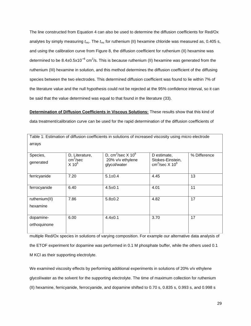
The line constructed from Equation 4 can also be used to determine the diffusion coefficients for Red/Ox

analytes by simply measuring tmc. The tmc for ruthenium (II) hexamine chloride was measured as, 0.405 s,

and using the calibration curve from Figure 8, the diffusion coefficient for ruthenium (II) hexamine was

determined to be 8.4±0.5x10─6

cm2/s. This is because ruthenium (II) hexamine was generated from the

ruthenium (III) hexamine in solution, and this method determines the diffusion coefficient of the diffusing

species between the two electrodes. This determined diffusion coefficient was found to lie within 7% of

the literature value and the null hypothesis could not be rejected at the 95% confidence interval, so it can

be said that the value determined was equal to that found in the literature (33).

Determination of Diffusion Coefficients in Viscous Solutions: These results show that this kind of

data treatment/calibration curve can be used for the rapid determination of the diffusion coefficients of

multiple Red/Ox species in solutions of varying composition. For example our alternative data analysis of

the ETOF experiment for dopamine was performed in 0.1 M phosphate buffer, while the others used 0.1

M KCl as their supporting electrolyte.

We examined viscosity effects by performing additional experiments in solutions of 20% v/v ethylene

glycol/water as the solvent for the supporting electrolyte. The time of maximum collection for ruthenium

(II) hexamine, ferricyanide, ferrocyanide, and dopamine shifted to 0.70 s, 0.835 s, 0.993 s, and 0.998 s

Table 1: Estimation of diffusion coefficients in solutions of increased viscosity using micro electrode

arrays

Species,

generated

D, Literature, cm

2/sec

X 106

D, cm2/sec X 10

6

20% v/v ethylene glycol/water

D estimate, Stokes-Einstein, cm

2/sec X 10

6

% Difference

ferricyanide 7.20 5.1±0.4 4.45 13

ferrocyanide 6.40 4.5±0.1 4.01 11

ruthenium(II)

hexamine

7.86 5.8±0.2 4.82 17

dopamine-

orthoquinone

6.00 4.4±0.1 3.70 17

30

respectively. The calibration curve in Figure 8 was used in Figure 9 to determine diffusion coefficients of

each in the more viscous solutions (the green points in Figure 8). The diffusion coefficients determined for

ferri/ferro cyanide, dopamine and ruthenium hexamine in the more viscous solution were determined from

Figure 8 and are shown in Table 1.

As expected the diffusion coefficient for each of the Red/Ox analytes has decreased by approximately

30% in the more viscous solution. Because there are no literature values for the diffusion coefficients in

the more viscous solutions, we made estimates using the Stokes-Einstein equation: (50),

Figure 9: The determination of the diffusion coefficients of ferricyanide, ferrocyanide, ruthenium(II)

hexamine, and dopamine o-quinone (DOQ) through solutions with higher viscosity (20% v/v Ethylene

glycol/water). The original aqueous calibration curve (orange markers), a determined diffusion coefficient

for aqueous ruthenium (II) hexamine (blue marker), and the diffusion coefficients in increased viscosity

(green markers), based on the calibration shown in Figure 8.

31

Equation 6

Where D is the diffusion coefficient, T is the temperature, kb is Boltzmann’s Constant, r is the radius of the

spherical particle, and η is the viscosity of the solution. Predicted values for the diffusion coefficients in

the more viscous solutions are shown in the table, assuming that the change in solvent only affects the

viscosity. Other than the Stokes-Einstein equation there has been little theoretical work predicting how

diffusion coefficients should change with changes in viscosity. It has been shown that relative errors

between experimental and the theoretical prediction from Stokes-Einstein range between 12 and 35%

with more extreme errors possible based on the non-spherical nature of the particles that diffuse (50).

Dopamine o-quinone and ferrocyanide in figure 8, appear to have the same diffusion coefficients in the

20% v/v ethylene glycol/water solution. Ferrocyanide has the expected slower diffusion coefficient in the

more viscous solution, dopamine o-quinone however has a faster than expected diffusion coefficient. This

could be because of unexpected solvent effects between the dopamine and the 20% v/v ethylene glycol

solution altering the hydrated radius to smaller value. The determined diffusion coefficient for dopamine o-

quinone is still in the low end of the expected range of disagreement (12-35%) with the Stokes-Einstein

estimation.

Conclusions

This alternative treatment of ETOF can quickly determine many diffusion coefficients for Red/Ox

species from a single experiment. The method outlined here can be used to determine the diffusion

coefficients, as viscosity increases, empirically and swiftly. This method can also be used to determine if

diffusion coefficients predicted using the Stokes-Einstein equation make empirical sense. The percent

error between the diffusion coefficients estimated with Stokes-Einstein and the diffusion coefficients

determined empirically using our alternative method of ETOF was in the range of 11-17% error of the

predicted values, and the acceptable range of percent errors is from 12-35%(44). These values fall within

in the acceptable range, and were determined without expensive modeling software or time consuming

experiments.

Future applications could include determining diffusion coefficients through membranes. Since diffusion

32

coefficients through membranes set the sensitivity of amperometric sensors, we envision, this research

could be used to recalibrate implanted electrochemical sensors in biological applications, as well as a

variety of other applications. There are as yet other possible applications that have not been considered

because ETOF lacks the visibility needed for people to begin working on these important applications.

Acknowledgements

Arkansas Applied Biosciences Institute

Special thanks for Professor Ingrid Fritsch for her helpful discussions; and Mengia Hu and Nandita Halder

for the fabrication of microelectrode arrays.

References

1. G. Che, Z. Li, H. Zhang and C. R. Cabrera, J. Electroanal. Chem., 453, 9 (1998).

2. A. M. Lehaf, M. D. Moussallem and J. B. Schlenoff, Langmuir, 27, 4756 (2011).


4. R. A. Ghostine and J. B. Schlenoff, Langmuir, 27, 8241 (2011).

5. H. Dong, X. Cao and C. M. Li, ACS Appl. Mater. Interfaces, 1, 1599 (2009).

6. M. Strawski and M. Szklarczyk, J. Electroanal. Chem., 624, 39 (2008).

7. A. I. Bhatt and R. A. W. Dryfe, J. Electroanal. Chem., 584, 131 (2005).

8. A. I. Gopalan, K.-P. Lee, K. M. Manesh, P. Santhosh and J. H. Kim, J. Mol. Catal. A: Chem., 256, 335 (2006). 9. M. Etienne, A. Quach, D. Grosso, L. Nicole, C. Sanchez and A. Walcarius, Chem. Mater., 19, 844 (2007). 10. S. A. Rothwell, M. E. Kinsella, Z. M. Zain, P. A. Serra, G. Rocchitta, J. P. Lowry and R. D. O'Neill, Anal. Chem. (Washington, DC, U. S.), 81, 3911 (2009). 11. W.-F. Dong, S. Liu, L. Wan, G. Mao, D. G. Kurth and H. Moehwald, Chem. Mater., 17, 4992 (2005). 12. L. Motiei, R. Kaminker, M. Sassi and M. E. van der Boom, J. Am. Chem. Soc., 133, 14264 (2011).

13. C. M. Berger and C. L. Henderson, Proc. SPIE-Int. Soc. Opt. Eng., 5376, 392 (2004).

14. J. J. Harris and M. L. Bruening, Langmuir, 16, 2006 (2000).

15. H. Ding, Z. Pan, L. Pigani and R. Seeber, J. New Mater. Electrochem. Syst., 4, 61 (2001).

33

16. R. Tucceri, J. Electroanal. Chem., 633, 198 (2009)

17. M. J. Rodriguez Presa, L. M. Gassa, O. Azzaroni and C. A. Gervasi, Anal. Chem. (Washington, DC, U. S.), 81, 7936 (2009). 18. E. P. O'Brien and T. C. Ward, ASTM Spec. Tech. Publ., STP 1463, 72 (2005).

19. V. M. M. Lobo and M. H. S. F. Teixeira, Electrochim. Acta, 24, 565 (1979).

20. V. M. M. Lobo, M. Helena, S. F. Teixeira and J. L. Quaresma, Electrochim. Acta, 27, 1509 (1982).

21. V. M. M. Lobo and J. L. Quaresma, Electrochim. Acta, 35, 1433 (1990).

22. V. M. M. Lobo and A. J. M. Valente, Polym. Degrad. Stab., 44, 147 (1994).

23. V. M. M. Lobo, A. C. F. Ribeiro and A. J. M. Valente, Corros. Prot. Mater., 14, 14 (1995).

24. K. Tanaka, T. Hashitani and R. Tamamushi, Trans. Faraday Soc., 66, 74 (1970).

25. F. Liu, G. Kolesov and B. A. Parkinson, J. Electrochem. Soc., 161, H3015 (2014).

26. C. D. Johnson and D. W. Paul, Sens. Actuators, B, 105, 322 (2005).


28. C. Amatore, C. Sella and L. Thouin, J. Electroanal. Chem., 593, 194 (2006).

29. H. B. Tatistcheff, I. Fritsch-Faules and M. S. Wrighton, J. Phys. Chem., 97, 2732 (1993).

30. I. Fritsch-Faules and L. R. Faulkner, Anal. Chem., 64, 1118 (1992).

31. D. Ky, C. K. Liu, C. Marumoto, L. Castaneda and K. Slowinska, J. Controlled Release, 112, 214 (2006). 32. K. Slowinska, M. J. Johnson, M. Wittek, G. Moller and M. Majda, Proc. - Electrochem. Soc., 2001-18, 130 (2001). 33. S. Licht, V. Cammarata and M. S. Wrighton, J. Phys. Chem., 94, 6133 (1990).

34. R. D. Martin and P. R. Unwin, J. Electroanal. Chem., 439, 123 (1997).



37. C. G. Zoski, C. R. Luman, J. L. Fernandez and A. J. Bard, Anal. Chem. (Washington, DC, U. S.), 79, 4957 (2007). 38. C. G. Zoski, B. Liu and A. J. Bard, Anal. Chem., 76, 3646 (2004).


40. A. J. Bard, J. A. Crayston, G. P. Kittlesen, T. Varco Shea and M. S. Wrighton, Anal. Chem., 58, 2321 (1986). 41. M. Hu and I. Fritsch, Anal. Chem. (Washington, DC, U. S.), 87, 2029 (2015).

34

42. M. Shabrang and S. Bruckenstein, J. Electrochem. Soc., 121, 1439 (1974).

43. P. Hashemi, P. L. Walsh, T. S. Guillot, J. Gras-Najjar, P. Takmakov, F. T. Crews and R. M. Wightman, ACS Chemical Neuroscience, 2, 658 (2011). 44. S. J. Konopka and B. McDuffie, Anal. Chem., 42, 1741 (1970).

45. V. Cammarata, D. R. Talham, R. M. Crooks and M. S. Wrighton, J. Phys. Chem., 94, 2680 (1990). 46. A. Varga, G. Gyetvai, L. Nagy and G. Nagy, Anal. Bioanal. Chem., 394, 1955 (2009).

47. K. Slowinska, S. W. Feldberg and M. Majda, J. Electroanal. Chem., 554-555, 61 (2003).


49. G. Gerhardt and R. N. Adams, Anal. Chem., 54, 2618 (1982).

50. H. A. Kooijman, Ind. Eng. Chem. Res., 41, 3326 (2002).

35

Optimization of Electrochemical Time of Flight Measurements for Precise Measurements of

Diffusion Coefficients over a Wide Range in Various Media

Jonathan Moldenhauer, Catherine Sella*, Becca Moffett, Joel Baker, Laurent Thouin*, Christian

Amatore*, Stefan Kilyanek, and David W. Paul

Department of Chemistry and Biochemistry


1 University of Arkansas

Fayetteville, AR 72701

USA

* PASTEUR, Département de chimie, École normale supérieure,

PSL Research University,

Sorbonne Universités, UPMC Univ. Paris 06, CNRS,

75005 Paris, France

36

Abstract

Diffusion coefficients are an important physical property to both electrochemistry and the role they play in

sensors, batteries, and catalysis. Electrochemical Time of Flight (ETOF) is a powerful and elegant

technique that has largely been relegated to verifying diffusion modeling and theoretical work; instead of

seeing prominence for its ease of use and broad applicability. ETOF does not require setting delicate

hydrodynamic conditions that rotating ring disk (RDE) methods do, nor any mechanistic foreknowledge

that is required about the electrochemical system, making this ideal for determining the diffusion

coefficients for non-elucidated systems. Using experimental parameters optimized by computer

modeling, an empirical calibration was generated for a platinum micro electrode array, and diffusion

coefficients were determined for ferrocene, ruthenium(III) bisbipyridine dichloride, vanadyl

acetoacetonate, and tetrabutylammonium dioxovanadium(V) dipicolinate some of which were previously

unreported.

37

Introduction

In addition to being a fundamental property of any solute, diffusion coefficient values are crucial,

especially in several applications of electrochemistry. Diffusion plays a pivotal role in mechanistic

investigations as well as for amperometric and potentiometric sensors(1), electrosynthesis(2), redox flow

batteries(3), etc. These are all applications where the electrical response and/or the global outcome

depends on the diffusion of molecules to and from an electrode. Typically diffusion coefficients values, D,

are determined either by electrochemical means using scanning electrochemical microscopy (SECM)(4-

9), or by rotating ring disk (RDE) methods(10-17). RDE methods are based on the Levich equation,

equation 1. The RDE limiting diffusion current plateau value, ilev, is related to D but also to the number of

electrons transferred, n, the Faraday’s constant, F, the active area of the electrode, A, the diffusion

coefficient of the analyte (electroactive), D, the kinematic viscosity of the supporting electrolyte, ν, the

rotation rate, ω, the analyte concentration of the in bulk, Cs (12). When iLev values are plotted as a function

of √ , the slope containing multiple terms including the diffusion coefficient.

Equation 1

The issue is that the other terms in the slope must be known to calculate the diffusion coefficient, n, A, ν,

and Cs. Acquiring values for these terms can be a little troublesome: such as the active surface area of

the electrode, which could vary significantly from the geometric surface area; number of electrons

transferred that, due to specific mechanistic circumstances, may be constant but not be an exact

integer(18) or vary with the probed time range(19); kinematic viscosity of the solution; the concentration of

the analyte. All of these can be determined through additional experiments performed with the required

accuracy, but this makes for an additional burden. In addition, every electroactive analyte experiences

different diffusion coefficient values in different media. Using RDE to determine diffusion coefficients

requires a new Levich plot be constructed for each Red/Ox analyte every time any of the terms n, A, ν,

and Cs change, adding cumbersome details to the determination. Finally, it should be noted that equation

(1) relates to the diffusion coefficient of the bulk electroactive species and not to its product.

A variant of this principle was also introduced to determine simultaneous values of n and D for any

electrochemical wave through the combination of the limiting steady state current measured at an

38

ultramicroelectrode to the Cottrell current measured in the same solution at a millimetric electrode(19).

However the method requires a high experimental precision and accuracy and should then be reserved to

situations in which time-dependent kinetics may affect the then time-dependent n value.

In SECM, the probe serves as the detector electrode and is moved vertically to different distances from a

surface that is generating a redox active species. The diffusion coefficient is determined by measuring

the time of maximum collection at different distances from the surface. However such SECM-based

method may not be applicable in structured electrolyte media such as polymers or sol-gel materials in

which diffusion coefficient values may be required(17).

In fact, the very principle of such SECM experiments is similar to that of electrochemical time of flight

(ETOF) ones as both involve generation and collection of the species of interest. Electrochemical time of

flight (ETOF) was first developed by Royce Murray(20) to measure the time that a generated species took

to travel from one electrode to an adjacent detecting electrode located at a known distance away; the

travel time could then be related to the diffusion coefficient. Murray was interested in determining the

apparent diffusion coefficients of electron-hopping across conducting polymers sandwiched between two

electrodes (20). Hence, the SECM and ETOF approaches only differ from the fact that the former relies

on collector-generator current feedback magnitude (viz., on collection efficiencies(21)) while the second

one relies on measurements of travel times of the generated species of interest between its source (the

generator electrode) and its sink (the collector electrode(s)). This travel time, tmc is indeed related to the

diffusion coefficient, D, through Einstein’s equation, equation 2, the distance traveled or gap between the

electrodes, g, and a numerical dimensionless constant, K, that depends exclusively on the electrode array

geometry and not at all on the electrochemical medium.

√ Equation 2

K can be predicted by computational means for generator-collector systems having ideal geometries (22,

23) or evaluated empirically based on calibrations performed for micro-systems of any geometry(24-26).

Most of the literature has been reporting ETOF applications as a way to verify computational models of

diffusion between electrodes, viz., as a way to assess experimentally the “ideality” of the microfabricated

39

systems, but rarely as an extremely adequate and simple technique for determining diffusion coefficients.

Previously, transit times of analytes at different distances between the generating and detecting

electrodes were measured to determine diffusion coefficients with ETOF. These experiments have been

limited to model compounds such as ruthenium hexamine(23, 25), ferricyanide(22, 23), and

hydroxymethylferrocenium(27) for example, or the analyte of interest in a given study(24). The advantage

of ETOF over other methods is that it does not require the foreknowledge all the solution parameters

mentioned above, as required by RDE methods, nor does it require specialized equipment as SECM

does. Following the advent of mass produced microelectrode arrays and despite the simplicity of the

technique it is surprising that ETOF is not a standard method for determining unknown diffusion

coefficients.

In our previous work, we presented a novel data treatment for electrochemical time of flight

(ETOF) that we believe provided a simple and elegant method for determining diffusion coefficients. In

this approach a calibration curve is constructed by measuring tmc with a given micro-device (viz., for a

single and constant distance, g, between the generator and collector electrodes) for electrogenerated

species with known diffusion coefficients in the medium of interest. Rewriting equation 2 as follows.

√

√ Equation 3

Plotting √ variations as a function of

√ known values for species with reported diffusion coefficients,

produces a calibration line that can then be used to determine diffusion coefficients of unknowns species

regardless of other characteristics of the medium and of the species. In this paper we have expanded

electrolyte solutions to include non-aqueous solvents. In addition, computer modeling was used to

optimize the pulse widths for the generator, so that diffusion coefficients could be determined over a large

dynamic range with an adequate precision and accuracy.

Theoretical optimization of precision and accuracy in ETOF measurements

Generator-collector micro-devices may be used under steady state regimes(21, 23). Refering to Figure

10, it is clear relying on steady-state operation is not suitable since any information related to the time of

flight of the species B formed at the generator is lost, being somewhat convoluted with kinetic effects into

40

the common current intensities of the generator and collector electrode(s)(21). Conversely, applying a

sufficiently brief potential pulse(18,24) to the generator electrode generates a local concentration of B in

its very vicinity(28). Diffusional broadening of this concentration pulse over the insulating gap allows B to

be captured by the collector(s). though, since the duration of the generator pulse is brief, B is rapidly

exhausted. Hence, a peak-shaped current response is expected at the collector(22, 29) whose maximum

time position, tmc, is directly indicative of B shortest time-of-flight (TOF). Conversely, whenever the

electrochemical detection of B regenerates A, this latter species may then diffuse back to the generator

where it can regenerate B if the generator is still electrochemically active. This is bound to induce a

redox-cycling mechanism while the generator may perform. As a consequence, the time position of the

maximum collector current is deported towards large times since it now represents a convolution between

the shortest TOF and the maximization of the redox-cycling efficiency. Therefore, in absence of any noise

or background interference, the smallest is tpulse value the most accurate is the application of equations 2

and 3. Conversely, the shortest is tpulse, the smallest is the generated quantity of B and its electrochemical

current at the collectors, hence the lowest is the precision of tmc determination. This experimental conflict

between accuracy and precision indicates that tpulse value should be as close as possible from a maximum

one, , beyond which redox-cycling contributions will alter the ETOF measurements. However, it is

understood that this value is not universal but depends on the rate of diffusion of B over the insulating

gaps, viz., on tmc.

Therefore, though the present work is aimed to validate experimentally the principle of diffusion

coefficients measurements by ETOF and determine experimentally the specific calibration curve relating

D and tmc values (equation 3) for any given micro-device irrespective of the electrolyte medium in which

the measurements are performed, one needs first to estimate the relationship between and tmc

values in order to guarantee both the precision and the accuracy of the ETOF calibration curve for the

micro-device of interest. This is essential to ensure that the corresponding calibration curve may then

safely be used for determining the unknown diffusion coefficients of other species in any media with the

same micro-device. For this reason we wish to present the results of a simplified theoretical analysis

aimed to evaluate the relationship between and tmc values.

41

This theoretical analysis was performed through Comsol simulations of ideal micro-device systems

consisting of three parallel microband electrodes of common width, w, separated by insulating gaps of

common width g, the whole assembly being imbedded flat in an insulating plane (Figure 10A)(21, 30).

Owing to its scope, this theoretical analysis was simplified through considering that the electrodes present

no vertical edges and that no metallic conductor was located within the gap separating the generator and

collector electrodes in order to avoid theoretical complications related to any bipolar activity that may be

induced over such isolated conductors(31, 32).

Initially, the semi-infinite bulk electrolyte is assumed to contain only a species A. This is reduced, or

oxidized accordingly, at the generator electrode whose potential is stepped for a fixed time duration, tpulse,

at an adequate value and disconnected afterwards (Figure 10B). This generates a peak-shaped current

response (Figure 10C) characterized by its current maximum, imc, and its time position, tmc, after the

beginning of the pulse (t = 0).

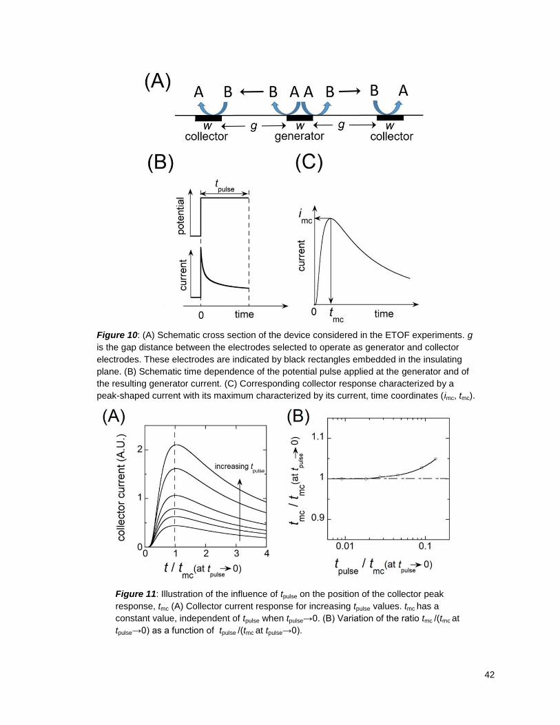
42

Figure 10: (A) Schematic cross section of the device considered in the ETOF experiments. g

is the gap distance between the electrodes selected to operate as generator and collector

electrodes. These electrodes are indicated by black rectangles embedded in the insulating

plane. (B) Schematic time dependence of the potential pulse applied at the generator and of

the resulting generator current. (C) Corresponding collector response characterized by a

peak-shaped current with its maximum characterized by its current, time coordinates (imc, tmc).

Figure 11: Illustration of the influence of tpulse on the position of the collector peak

response, tmc (A) Collector current response for increasing tpulse values. tmc has a

constant value, independent of tpulse when tpulse→0. (B) Variation of the ratio tmc /(tmc at

tpulse→0) as a function of tpulse /(tmc at tpulse→0).

43

Figure 11A illustrates the outcome of the corresponding simulations by evidencing how the collector

peak-shaped response vary when tpulse increases. Figure 11B reports the variations of tmc normalized to

its ideal limit when tpulse → 0, as a function of tpulse also normalized to the same limit. This dimensionless

presentation of the theoretical results makes that Figure 11B is independent of the exact nature of the

redox system A/B considered and of the geometry of micro-device used provided that its geometric

characteristics approach closely the ideal ones defined above. Also, since the generator and collector

potentials may be experimentally chosen so that the reduction of A, or its oxidation accordingly, and the

detection of B are performed at the current plateaus of the corresponding electrochemical waves, Figure

11B is independent of the exact mechanisms involved during these electrochemical processes provided

that species B is the one that diffuses over the micro-device gaps. In other words, would B be a follow-up

product resulting from the chemical evolution of A±, the primary intermediate formed by the reduction of A,

or its oxidation accordingly, the half-life time, t1/2

, of the formation of B from A± must be negligible vs. tmc.

Would that not be the case, the ETOF method would provide a “mixed” diffusion coefficient convoluting

those of B and A±. In order to guarantee that this is not the case, the ETOF method should be reserved to

the analysis of redox systems that are not necessarily reversible but whose CV simultaneously displays

the voltammetric waves of A (forward scan) and B (backward scan) and no intermediate wave within a

single voltammetric scan performed at a scan rate, v, matching tmc, viz. such as vmc ~ RT/(Ftmc) where R

is the perfect gas constant, F the Faraday number, and T the absolute temperature(33).

A first conclusion of this simplified theoretical analysis described in this section, shows that the

optimization of its accuracy and precision imposes (Figure 11B) that the duration of the generator pulse

duration, tpulse, does not exceed a maximum value being ca. 0.03 to 0.04 times that of the experimentally

determined tmc. The validity of this criterion must therefore be verified after a given determination of tmc in

order to ensure the validity of the correspondingly determined diffusion coefficient value. A second

conclusion is that the ETOF method applies to determine the diffusion coefficient of any species that is

the primary intermediate of the reduction or oxidation of a precursor species, A, or is generated from this

primary intermediate within a time-scale t1/2

that is much shorter than tmc. The exact relationship between

the maximum value, (t1/2

)max, of t1/2

and tmc is evidently depending on the mechanism relating B to the

primary intermediate A±, but the use of equation 3 should provide correct results when t

1/2 < tmc.

44

Experimental

Hardware: All electrochemical measurements were performed using a CHInstruments 750a

bipotentiostat, and an in-house built circuit to control the generator electrodes. The in-house circuit was

controlled by National Instruments LabVIEW software. The micro band electrode arrays of 16 platinum or

gold fingers, 2 mm long, 25 μm wide with gaps of 25 μm were fabricated at the Arkansas High Density

Electronics Center(HiDEC). Using either one of these arrays provided essentially identical results. An

Ag/AgCl in saturated KCl reference electrode was used in aqueous solutions. For use in organic solvents

a bridge, made with TBAPF6 in acetonitrile was constructed over a SCE.

Chemicals: Potassium ferrocyanide (Certified ACS grade, Fischer), potassium ferricyanide (Certified

ACS grade, Fischer), ruthenium (III) hexamine chloride (highest purity available, Alfa Aesar), ferrocene

(98% Sigma Aldrich), ferrocenyl acetic acid (98% Sigma Aldrich), ruthenium bisbipyridine dichloride

(Ru(bpy)2Cl2) (97% Sigma Aldrich) were all obtained and used as received unknowns were all obtained

and used as received to make 5 mM solutions in the chosen electrolyte. Two solutions were considered.

One (aqueous) consisted of 0.1 M KCl (ACS grade, J.T. Baker). The other (organic) consisted of 0.1 M

TBAPF6 (98%, Sigma Aldrich) in acetonitrile (HPLC Grade, Fischer).

The vanadyl acetylacetonate (VO(acac)2) was synthesized from Vanadium(V) Oxide (98%, Sigma

Aldrich) and acetylacetone (Reagent Plus grade, Sigma Aldrich) according to the method below and was

recrystallized for purification in dichloromethane(34). Note however that VO(acac)2 oxidation has been

reported to provide very rapidly VO(acac)3, especially if the solution contains already traces of

VO(acac)3(35). The presence of VO(acac)3 traces in our synthesized VO(acac)2 samples was confirmed

by comparing the infra-red spectra of the solution of our synthesized VO(acac)2 with that reported for a

pure VO(acac)2 solution (Sigma Aldrich).

The tetrabutylammonium dioxovanadium(V) dipicolinate (VO2(dipic)) synthesis proceeded as follows. A

tetrabutylammonium hydroxide ([n-Bu4N]OH) solution was prepared by diluting 100mL of 40% wt. in H2O

(Aldrich) to 1 liter with deionized water to yield a 0.4M solution. Approximately 4.0g of solid V2O5 (≥98%,

Aldrich) was added to 200mL 0.4M [n-Bu4N]OH in a 500mL Erlenmeyer flask and left to stir for

approximately 18 hours at room temperature. The solution changed from a transparent yellow to nearly

45

colorless liquid with a very small amount of colorless solid floating on the top. The solid was vacuum-

filtered from the solution using a Buchner funnel and the remaining filtrate transferred to a 250mL round

bottom flask. The filtrate was then dried on a rotary evaporator for 1-2 hours at 46° C until the appearance

of viscous, light-brown oil. The round bottom flask was placed on a Schlenk line and left overnight to

evaporate to complete dryness, yielding a crude, white solid. The flask was then back-filled with nitrogen,

sealed, and transferred to a glovebox under a nitrogen atmosphere for extraction of the air-sensitive

intermediate, [n-Bu4N][VO3](36).

To complete the synthesis of VO2(dipic), approximately 1 gram of the [n-Bu4N][VO3], 0.5g 2,6-pyridine

dicarboxylic acid (99%, Aldrich), and 3g 4Å molecular sieves were placed in 15-20mL dichloromethane

(99.8%, anhydrous, Sigma-Aldrich) and left to stir for ~45 minutes. The sieves and insoluble solid were

vacuum-filtered using a fritted funnel and flask. The remaining filtrate was then pumped down to ~4mL,

layered with diethyl ether (dried, Sigma-Aldrich), and placed in the glovebox freezer for crystallization.

After seven days the mother liquor was decanted and the wet crystals dried under vacuum. The

crystalline solid was then transferred to a clean vial, triturated with fresh diethyl ether, dried again under

vacuum and then weighed. Typical final product yield: 0.88-0.92 grams(37) of VO2(dipic).

Conditions of electrochemical measurements:

Three equally spaced (gap distance of g=75µm) microband electrodes (w=25µm) was selected by pairing

sets of microbands available in the microfabricated arrays to perform ETOF measurements. The other 13

microbands present in the array were not connected. The generator electrode potential was imposed

during a time duration, tpulse, and the generator immediately disconnected to minimize current feedback.

The two collector electrodes remained continuously poised(30).

The applied potentials values were determined from CVs of reported for the A/B couples performed in 0.1

M KCl or in 0.1 M TBAPF6 / acetonitrile. For the latter case, unless otherwise noted, all potentials were

measured versus a SCE with a double bridge. The potential window for the CV for ferrocene and

ferrocenyl acetic acid solutions was from -0.6 V to +0.8 V, and the ETOF potentials were selected as

follows: for ferrocenium, the generator was pulsed to +0.8 V while the collectors were held at +0.1 V. For

46

experiments with ferrocenyl acetic acid, the generator was pulsed to +0.5 V while the collectors were held

at 0.1 V. The CV potential window for Ru(II)(bpy)2Cl2 was +0.5 V to -0.2 V and the ETOF potentials set at

+0.5 V for the generator pulse and -0.1 V for the collectors. The ferrocene/ferrocenium had a known

diffusion coefficient in the literature(38) and Ru(II)(bpy)2Cl2 was compared to an estimated diffusion

based on its mass(39).

VO2(dipic) electrochemical reduction forms a dimer when there are proton donating buffers such as tosic

acid. So, the diffusion coefficient of the reduced form of this dimer was determined in acetonitrile with 0.1

M electrolyte TBAPF6 and the tosic acid buffer 0.0150M. The VO2(dipic) / VO2(dipic) dimer couple is not a

reversible redox one as the above ones. The voltammetric potential window was then extended over the

range +1.6 V to -1.6 V vs a silver cryptand reference to identify the VO2(dipic) reduction wave and the

oxidation one of the VO2(dipic) dimer. This enabled selecting ETOF potentials as +0.4 V for the generator

pulse and +0.9 V for the collectors. The diffusion coefficient of the dimer was determined experimentally

using ETOF and compared with those of the dimer determined by other by using Koutecky-Levich plots.

The mechanism undergoing at the VIV

O(acac)2 oxidation wave is even more complex, leading to

VVO(acac)3 (see below in Results and Discussion). The potential window for the CV of VO(acac)2 was

thus extended from +2.0 V to -2.0 V to identify the ETOF potentials. These were set at +1.0 V for the

generator pulse and -1.5 V for the collectors in order to determine the diffusion coefficient of VO(acac)3.

47

Results and Discussion

An experimental ETOF calibration curve (Figure 12) was determined as reported before(30) using a

constant value of tpulse = 61 ms using either gold or platinum band electrodes. The calibration curve was

constructed based on the experimental √ values determined in 0.1 M KCl for ferrocyanide (6.40 x 10─6

cm2/s)(23), ferricyanide (7.20 x 10

─6 cm

2/s)(40) and ruthenium(II) hexamine (7.86 x 10

─6 cm

2/s)(23)

whose D values are reported in the literature. The regression line, √ = 3.23(±0.03)x10-3

/√ , was

determined by enforcing it to pass through the origin in order to comply with the theory (18). From

equation 3 and g=75µm, this slope provided K = 2.32(±0.02). It was also verified that for the three species

Figure 12: Calibration curve constructed using standards compounds ferrocyanide, ferricyanide,

and ruthenium (II) hexamine in 0.1 M KCl aqueous solution (blue points) based on their tmc values

determined from ETOF experiments using tpulse = 61ms and known diffusion coefficients. The

dotted line represents the equation √ = 3.23(±0.03)x10-3

/√ . The incorrect tmc values

determined for ferrocene and ferrocenyl acetic acid in acetonitrile using tpulse = 61ms are shown by

orange circles while the correct one measured for ferrocene using tpulse = 24ms is shown by a

green point.

48

used as calibrants, using tpulse = 61 ms satisfied the criterion developed above. Indeed, based on the

experimental tmc values, one had tpulse/tmc = 0.037 (ferrocyanide), 0.042 (ferricyanide) and 0.046

(ruthenium(II) hexamine), which is satisfactory owing to the theoretical results in Figure 11B.

Using, this calibration curve the diffusion coefficients values for ferrocene and ferrocenyl acetic acid could

be determined based on their tmc values. However, the case of ferrocene served to illustrate the danger of

using too large values for tpulse. Indeed, ferrocene reported to have a larger diffusion coefficient,

2.24(±0.07)x10-5

cm2/s(28), than those used to construct the calibration line in Figure 12. Using the same

pulse width tpulse = 61 ms gave a tmc value of 0.93 s, which the calibration curve translated as diffusion

coefficient of 1.22(±0.03)x10-5

cm2/s for ferrocenium, being then in strong contrast with the value of

2.24(±0.07)x10-5

cm2/s reported in the literature (38). A similarly wrong outcome was obtained for the

diffusion coefficient of ferrocenyl acetic acid. Using again tpulse = 61 ms afforded D = 1.10(±0.05)x10-5

cm2/s upon using calibration line in Figure 12 while a diffusion coefficient of 1.92x10

-5 cm

2/s is predicted

for ferrrocenyl acetic acid based on its molecular weight(39). In fact, the two species diffuse too rapidly for

using a tpulse = 61 ms value in the ETOF experiments. tpulse was thus decreased from 61 ms to 24 ms in

order to satisfy the above criterion (tpulse/tmc = 0.037). Using tpulse = 24 ms afforded a diffusion coefficient

value of 2.4(±0.1)x10-5

cm2/s (see e.g. the relative positions of the two corresponding data point for

ferrocene in Figure 12) for ferricinium being within 7% of the reported literature value for that of ferrocene

at room temperature in acetonitrile(28). This illustrates the importance of verifying a posteriori that the

tpulse/tmc criterion was satisfied after tmc has been determined for the selected tpulse value.

Aqueous Diffusion Coefficient Calibration Curves Can Extend to Organic Solvents

The calibration curve in Figure 12 was constructed using literature data values (Ds) and measured ones

(tmcs) in 0.1 M KCl. However, the value of the constant K is an intrinsic characteristic of the micro-device

and not of the redox system investigated or the electrolyte medium used. Hence, the calibration curve in

Figure 12 is expected to be valid in all electrolytes even if it was constructed using specific redox systems

in 0.1M KCl. To test the validity of this prediction, ETOF measurements were performed in 0.1 M TBAPF6

/ acetonitrile for ferrocene, Ru(bpy2)Cl2 and the VO2(dipic) dimer and their diffusion coefficients compared

49

to those reported in the literature or determined using RDE for the VO2(dipic) dimer. The corresponding

results are reported in Figure 13 in which the regression line is that determined in 0.1 M KCl in Figure 12.

As indicated above, the ETOF result for ferrocene matched perfectly the literature data(38). The same

was true for Ru(bpy2)Cl2(39), D = 9.3(±0.4)x10─6

cm2/s. This validates our claim that calibration curves

constructed using standard mediators in aqueous electrolyte, can be used to determine diffusion

coefficients in other electrolytes including organic media.

For the VO2(dipic) dimer a 3.9(±0.2) x 10─6

cm2/s value was obtained based on ETOF (see Figure 13)

being in excellent agreement with that, 3.94 x 10─6

cm2/s, determined using the slope of the Koutecky-

Levich plots (equation 1, with a 95% confidence level) deduced from RDE experiments performed on the

Figure 13: Use of the calibration curve reported in Figure 3 for 0.1 M KCl to determine diffusion

coefficients from tmc values determined in acetonitrile with 0.1 M TBAPF6 as the supporting

electrolyte for Ferrocene, Ru(bpy2)Cl2, VO(acac)3, and VO2(dipic); for Ferrocene, tpulse = 24 ms

was used while tpulse = 61 ms was used for the three other species. Blue circles represent the set

of data determined for Ru(NH3)63+

, Fe(CN)63-

and Fe(CN)64-

in 0.1 M KCl aqueous solution, while

orange circles represent the set of data determined in in acetonitrile / 0.1 M TBAPF6.

50

VO2(dipic) dimer. This latter example evidenced that the ETOF method is not at all restricted to A/B redox

systems that involve a single reversible electron transfer step but is applicable to more complex kinetic

sequences (see also below the case of VO(acac)2).

Application to VO(acac)2 in acetonitrile / 0.1 M TBAPF6

As recalled in the Experimental section, the electrochemical oxidation of vanadyl acetylacetonate,

VO(acac)2, samples is reported to easily lead to VO(acac)3 (30). This was confirmed through cyclic

voltammetry since the VO(acac)2 oxidation wave was irreversible and that of VO(acac)3 alone was

observed during the backward CV scan.

The present ETOF method amounts to determine the diffusion coefficient of the species generated at the

generator and not of that present in the solution bulk. So, the VO(acac)2 / VO(acac)3 dichotomy offered a

good opportunity to test the applicability of ETOF when the electron stoichiometry of the electrochemical

reaction producing the species of interest (here VO(acac)3) is complex and a priori unknown under

analytical conditions.

The electron stoichiometry of VO(acac)2 oxidation at the generator electrode is expected to generate the

cation VO(acac)2+ as the primary intermediate (the oxidation numbers of the vanadium center are noted in

the following to help checking the father-son sequences):

VIV

O(acac)2 – e VVO(acac)2

+ Equation 8

The highly chemical instability of this primary intermediate was confirmed by the chemically irreversible

CV oxidation wave of VIV

O(acac)2. Owing to the reported instability of VIV

O(acac)2 in the presence of

traces of its oxidation product VVO(acac)3 (30) and the irreversibility of the CV wave of V

IVO(acac)2,

VVO(acac)2

+ is expected to undergo a rapid father-son follow-up mechanism(18):

VVO(acac)2

+ + V

IVO(acac)2 → V

VO(acac)3 + V

IVO(acac)

+ Equation 9

Equation 9 affords the neutral VVO(acac)3 species whose diffusion over the generator-collector(s) gap

would then be measured instead of that of the primary oxidation intermediate VO(acac)2+. Note that the

51

overall electron stoichiometry of the mechanism in equations 8,9 is equal to 0.5 since one unreacted

VIV

O(acac)2 is consumed by the ligand exchange in equation 9:

VIV

O(acac)2 – 0.5 e → 0.5 VVO(acac)3 + 0.5 V

IVO(acac)

+ Equation 10

This global stoichiometry would even be more complex if VIV

O(acac)+ is oxidizable at the oxidation wave

of VIV

O(acac)2:

VIV

O(acac)+ – e V

VO(acac)

2+ Equation 11

as suggested by the absence of a reduction wave that could be ascribed to this species in the CV of the

VIV

O(acac)2 / VVO(acac)3 redox system. This may look unlikely at first glance owing to the coulombic

repulsion due to its positive charge. However, one expects that the resulting VVO(acac)

2+ species reacts

much faster with the parent VIV

O(acac)2 species than does VVO(acac)2

+:

VVO(acac)

2+ + 2 V

IVO(acac)2 → V

VO(acac)3 + 2 V

IVO(acac)

+ Equation 12

Equation 12 may thus displace the oxidation wave of VIV

O(acac)+ much before its standard potential(41)

so that it may occur before that of VIV

O(acac)2, so that a global father-son ECECE sequence takes place

at the potential of the VIV

O(acac)2 oxidation wave, thus leading to the global stoichiometric outcome in

equation 13:

VIV

O(acac)2 – (2/3) e → (2/3) VVO(acac)3 +(1/3) [V

IVO] Equation 13

where [VIV

O] represents unreacted ‘VIV

O’ vanadyl species and electrochemically inert over the -2V, 2 V

potential range voltammetrically explored.

In other words, depending on the extent of the conversion in equation 13, the electron stoichiometry of

VIV

O(acac)2 is expected to range between 0.5 and 2/3 of an electron per vanadyl center. This evidences

that relying on RDE measurements of VIV

O(acac)2 oxidation and Levich’s current limit to extract a

diffusion coefficient is necessarily biased by an unknown factor. Indeed, owing to equation 1, the Levich

current slope depends on the value of p = D2/3

n, hence the exact D value is extremely sensitive on the

actual value of (D = (p/n)1.5

.

52

Therefore, this redox system precisely served our purpose of illustrating a great specific advantage of the

ETOF method vs. the traditional RDE or SECM approaches. Indeed, using the limiting plateau current in

RDE would require a foreknowledge of the value, n, of the apparent number of electrons exchanged per

VO(acac)2. Similarly, current feedback measurements in SECM are highly dependent on the ability of

VO(acac)2 to be quantitatively regenerated by reduction of VO(acac)3 at the collector. Conversely, ETOF

measurements rely exclusively on diffusional time durations of the VO(acac)3 species and not at all on

current intensities.

The diffusion coefficient of VO(acac)3 in acetonitrile with 0.1 M TBAPF6 as the supporting electrolyte was

thus deduced experimentally based on the corresponding tmc value using the calibration curve without any

hypothesis about its exact nature. This afforded a value of 1.71(±0.08)x10─6

cm2/s (Figure 4). In

agreement with the complex mechanism detailed above, such value is in total disagreement with the

estimated diffusion coefficient based on the molecular weight of VIV

O(acac)2, viz., of its primary oxidation

intermediate VVO(acac)2

+. Conversely, a diffusion coefficient has been reported for V

VO(acac)3 (3), viz.,

2.3x10─6

cm2/s, being only 25% larger than the value measured by ETOF. Hence, it is presumable that

the species whose diffusion coefficient was determined by ETOF was VVO(acac)3.

Conclusions

This paper shows that ETOF is an elegant, effective, and simple method that can be used to easily

determine the diffusion coefficient of the product of a redox reaction even when this is form through a

complex mechanistic sequence. Indeed, the ETOF approach relies only on the duration of the diffusional

transport between a generator electrode where the species of interested is formed and one or two

collector electrode(s) at which it can be detected electrochemically and not at all onto electrochemical

current intensities. This contrasts with other approaches such as that using the Levich limit of RDE

currents or as SECM that relies on current feedback magnitude. This unique advantage of the ETOF

approach has been successfully illustrated in the context of vanadyl acetylacetonate, VO(acac)2,

oxidation that underwent a complex mechanism with unknown fractional electron stoichiometry.

Irrespective of this value, the diffusion coefficient of VO(acac)3, the stable oxidation product of this

53

complex oxidation wave, could be determined and shown to be in good agreement with a previously

reported value.

A second unique advantage of the ETOF method is that the relationship between the time of flight, tmc,

measurements and the sought diffusion coefficients, D, is independent of the electrolyte / solvent media

in which the ETOF measurements are performed, but depends exclusively on the geometrical

characteristics of the micro-device used for ETOF experiments. This has been illustrated by establishing a

calibration curve, √ √ (Figure 3), based on the measurements of tmc values in 0.1 M KCl for a

series of species whose diffusion coefficients were reported in the literature, and validating its use in 0.1

M TBAPF6 / acetonitrile (Figure 13).

Albeit these important and unique advantages, it is emphasized that a proper use of the ETOF method

requires that the duration, tpulse, of the potential pulse applied to the generator electrode is not excessively

long compared to the experimental time of flight, tmc. This is an essential criterion for guaranteeing a total

absence of diffusion cross-talk between the collector electrode(s) and the generator one which,

otherwise, would introduce significant biases in the ETOF measurements based on equations 2 and 3.

This important caveat has been illustrated based on two ETOF measurements performed for ferrocene in

0.1 M KCl at two different tpulse values, one of which was too large to satisfy this criterion and provided a

too small D value compared to published ones.

In this respect it is worth to mention that the whole ETOF experiments can be readily modeled using

commercial softwares such as Comsol so as to validate quantitatively the experimental calibration curve

corresponding to a given micro-device, as well as for establishing quantitatively the criterion fixing the

upper limit of tpulse values for a given experimental value of the time-of-flight tmc.

Acknowledgements

In Fayetteville, this work was supported by the Arkansas Applied Biosciences Institute and the National

Science Foundation (CHE-1263119/REU). In Paris, this work was supported by in parts by PSL, Ecole

Normale Supérieure, CNRS, and the University Pierre and Marie Curie (UMR 8640). Jonathan

Moldenhauer specially thanks Professor Ingrid Fritsch for helpful discussions, Dr. Stefan Kilyanek for

54

allowing Jonathan Moldenhauer to work with his graduate student and their glove box; and also Nandita

Halder & Errol Porter for the fabrication of microelectrode arrays.

References


2. C. Amatore and J. M. Saveant, J. Electroanal. Chem. Interfacial Electrochem., 126, 1 (1981).

3. Q. Liu, A. E. S. Sleightholme, A. A. Shinkle, Y. Li and L. T. Thompson, Electrochem. Commun.,

11, 2312 (2009).



6. R. D. Martin and P. R. Unwin, J. Electroanal. Chem., 439, 123 (1997).


8. C. G. Zoski, B. Liu and A. J. Bard, Anal. Chem., 76, 3646 (2004).

9. C. G. Zoski, C. R. Luman, J. L. Fernandez and A. J. Bard, Anal. Chem. (Washington, DC, U. S.),

79, 4957 (2007).

10. G. Che, Z. Li, H. Zhang and C. R. Cabrera, J. Electroanal. Chem., 453, 9 (1998).







17. A. I. Gopalan, K.-P. Lee, K. M. Manesh, P. Santhosh and J. H. Kim, J. Mol. Catal. A: Chem., 256,

335 (2006).

18. C. Amatore, G. Capobianco, G. Farnia, G. Sandona, J. M. Saveant, M. G. Severin and E.

Vianello, J. Am. Chem. Soc., 107, 1815 (1985).

19. C. Amatore, M. Azzabi, P. Calas, A. Jutand, C. Lefrou and Y. Rollin, J. Electroanal. Chem.

Interfacial Electrochem., 288, 45 (1990).


21. B. Fosset, C. Amatore, J. Bartelt and R. M. Wightman, Anal. Chem., 63, 1403 (1991).


55

23. S. Licht, V. Cammarata and M. S. Wrighton, J. Phys. Chem., 94, 6133 (1990).

24. D. Ky, C. K. Liu, C. Marumoto, L. Castaneda and K. Slowinska, J. Controlled Release, 112, 214

(2006).

25. K. Slowinska, M. J. Johnson, M. Wittek, G. Moller and M. Majda, Proc. - Electrochem. Soc., 2001-

18, 130 (2001).


27. H. B. Tatistcheff, I. Fritsch-Faules and M. S. Wrighton, J. Phys. Chem., 97, 2732 (1993).

28. N. Baltes, L. Thouin, C. Amatore and J. Heinze, Angew. Chem., Int. Ed., 43, 1431 (2004).

29. C. Amatore, N. Da Mota, C. Sella and L. Thouin, Anal. Chem. (Washington, DC, U. S.), 80, 4976

(2008).

30. J. Moldenhauer, M. Meier and D. W. Paul, J. Electrochem. Soc., 163, H672 (2016).

31. S. E. Fosdick, K. N. Knust, K. Scida and R. M. Crooks, Angew. Chem., Int. Ed., 52, 10438 (2013).

32. A. Oleinick, J. Yan, B. Mao, I. Svir and C. Amatore, ChemElectroChem, 3, 487 (2016).

33. C. Amatore, Y. Bouret, E. Maisonhaute, J. I. Goldsmith and H. D. Abruna, ChemPhysChem, 2,

130 (2001).

34. A. Vincent, Educ. Chem., 34, 165 (1997).

35. M. A. Nawi and T. L. Riechel, Inorg. Chem., 20, 1974 (1981).

36. G. Chapman, Jr. and K. M. Nicholas, Chem. Commun. (Cambridge, U. K.), 49, 8199 (2013).

37. V. W. Day, W. G. Klemperer and A. Yagasaki, Chem. Lett., 1267 (1990).

38. N. G. Tsierkezos, J. Solution Chem., 36, 289 (2007).

39. D. P. Valencia and F. J. Gonzalez, J. Electroanal. Chem., 681, 121 (2012).

40. S. J. Konopka and B. McDuffie, Anal. Chem., 42, 1741 (1970).

41. L. Nadjo and J. M. Saveant, J. Electroanal. Chem. Interfacial Electrochem., 48, 113 (1973).

56

Future Prospects and Conclusions

Recalibration of Oxygen Sensing Electrodes

The development of a tool for determining performance changes in both oxygen and enzyme electrodes

would make a significant impact on the development of sensors that are constructed with membrane

coverings. Since so much of the performance of these sensors depends upon membrane permeability, a

new method to determine the diffusion rate of molecules through membranes would have a broad impact.

These advancements would lay the ground work for obtaining more accurate results in clinical

applications involving implanted electrodes, providing a novel way to recalibrate electrodes in vivo. This

should allow for more accurate real-time measurements of analytes in clinical studies. It could also be

used in other situations where the electrodes are damaged by the in situ situation, such as probing for

oxygen in deep water or cooling water in a power plant.

Electrodes have been used to determine the oxygen concentration in vivo. The most common electrodes

used for this are based on the Clark type electrode. At a fundamental level, the sensitivity of the Clark

type electrode is set by the permeability of the membrane that covers the electrode(1). In addition, when

used in vivo, the membrane layer becomes fouled by non-specific adsorption, and the immune response

will eventually encapsulate the electrode. It can take a week for encapsulation to occur and before that

changes in membrane permeability with protein fouling cause changes in sensitivity, not only for the Clark

type oxygen electrode but for many types of electrochemical sensors that use a membrane coating(1).

The present method for calibration of electrodes in vivo and in situ electrodes is to use an external

calibration, then implant the electrodes into the desired environment. The calibration used in vitro is

expected to hold when used in vivo. This is rarely the case because the matrix of the analyte is often

dissimilar to the matrix of the calibration solutions(2). When placed in living tissue, non-specific adsorption

onto the membrane changes the permeability of the membrane and the rate at which analytes can

approach the electrode's surface, thus shifting in the sensitivity. Not correcting for the shift in sensitivity

after implantation causes errors in the concentrations reported by the probe(1). Quantitatively measuring

changes in membrane permeability could be used to improve the accuracy of the calibration of electrodes

that are being used for in vivo analysis.

57

There are non-electrochemical ways to accomplish this, such as light scattering spectroscopy, NMR

spectroscopy, and by using radioactive tracers(3). However, diffusion through membranes is usually

determined using electrochemical methods, the most popular being cyclic voltammetry at rotating disk

electrodes(RDE’s)(4). Impedance spectroscopy(5), non-rotated cyclic voltammetry(6), and wall jet

chronoamperometry(7) are also popular choices.

A Brief Comparison of ETOF to Other Methods for determination of Diffusion through membranes

Electrochemical time of flight (ETOF) is an electrochemical technique in which an analyte is generated

either oxidatively or reductively at one electrode, called the generator; it is detected by re-reducing/re-

oxidizing the analyte at a second electrode, called the collector. The time, tmax, that it takes the analyte to

travel from the center of the generator to the nearest edge of the collector, d, is the time of flight. By

measuring the time of flight, one can then determine the diffusion coefficient through the bulk solution.

ETOF could also be developed to determine the diffusion coefficient of analytes through a membrane that

coats the surface of the electrode. Quantitating diffusion coefficients of analytes thought membranes

would be useful for investigating changes in membrane permeability after biofouling. It would provide a

method of in situ recalibration of oxygen electrodes, at least for oxygen as previously reported with macro

electrodes(1). Recalibration of an oxygen sensor has been accomplished using macro electrodes, but

not with ETOF. However presently there are gaps in the literature that have previously prevented one

from being able to utilize ETOF to its fullest extent and in this dissertation I presented my work that turns

ETOF from a novelty into a full-fledged technique that should inable it to become a standard method for

the determination of diffusion coefficients.

However one place where ETOF has not been previously used is in the determination of diffusion

coefficients and permeabilities through membranes that have been polymerized on the surface of an

electrode. Determining the permeability and diffusion of electroactive molecules through membranes has

been done with cyclic voltammetry (CV), rotating disk electrodes (RDEs)(8-14) or rotating ring disk

electrodes (RRDEs)(15). Some qualitative work can be done by just looking at a change in the CV (16-

18) of a probe molecule. More quantitative investigations can be done using wall jet

chronoamperometry(7) or impedance spectroscopy(5, 19-23). But the majority of investigations into the

58

interactions of electroactive molecules and membranes have been done with RDE and/or cyclic

voltammetry.

Cyclic voltammetry even without using rotating disk electrodes has been used to evaluate the differences

in diffusion through defect sites on a polymer and the diffusion through the rest of the polymer layer(8).

One paper has shown that there are differences in the voltamagrams of a probe molecule between

through-film transport and pinhole (pore) diffusion(6). Through film transport means that the molecule is

dissolved into the film and then diffuses to the electrode, while in pinhole/pore diffusion the molecule

transports through evenly distributed pores or pinholes in the polymer across the surface of the electrode.

It is very important to know which kind of transport across the membrane is occurring if one wants to be

able to determine whether or not a complete coating over the surface of the electrode exists or if there are

defects spread across the surface. There are three different types of cyclic voltamagrams observed on

membrane covered electrodes, with varying scan rate. These responses are a) Randles-Ševčík, b)

steady-state and, c) thin layer. Randles-Ševčík responses are characterized by the fact that the

calculated peak current density (jpeak) is a function of square root of the dimensionless scan-rate(σ), γ the

diffusion coefficient ratio (

) of the analyte, Keq is the equilibrium constant between the analyte in

the solution and in the film, Equation 1.

√ . Equation 1

Steady State is the region where peak current as a function of scan rate is described by Equation 2, and

the thin film region’s peak current is described by the following equation Equation 3.(6)

Equation 2

: (

) Equation 3

By watching how the peak current changes as scan rates are shifted over at least three orders of

magnitude, one can infer the structure of the electroinactive polymer layer. This is because the thin layer

behavior is only exhibited in the case of through-film transport(6). Cyclic voltammetry by itself can also be

used for the gathering of preliminary data and qualitative investigations of diffusion(7, 16-18). This can be

59

done by noting qualitative changes in the shape and height of the peaks of the i-E curve with membrane

thickness or with the presence of a membrane compared to a bare electroce.(17). When polymers are

placed over electrodes raised off the substrate (as in the case of MEAs prepared by lithography), CV can

reveal slight differences in diffusion through the polymer located at the electrode’s edge(16). It can also

be used to examine a membranes exclusion to a given probe molecule and how the membrane affects

molecules with different polarities and charges, as well as differences in molecular construction of the

membrane in question(7).

Data from RDEs can be used to determine diffusion coefficients in bulk solution by using the Levich

equation. The Levich equation can also be applied to the diffusion of molecules through membranes that

have been polymerized on the surface of the RDE electrode(4). By using a probe molecule, the most

common being ferricyanide or hexamine ruthenium, one can investigate the permeability of the

membrane to these molecules, either by using a Levich plot or an inverse Levich plot (Koutecky-Levich

plot). These methods have been successful for numerous different membranes polyethylene

terephthalate(14), poly(allylamine)/poly(acrylic acid) crosslinkages(9), poly diallyldimethylammonium(11),

polystyrenes(10, 24), polypyrrole(12), metalopolymers(25),etc..) and various probe molecules other than

ferri-ferrocyanide and hexamine ruthenium,

including iodine(9) and quinones(14) in

aprotic solvents.

Another method to determine the

permeability/ diffusion of molecules

through a membrane is impedance

spectroscopy. A small sinusoidal potential

is used, as opposed to the much larger

potential window that is used by cyclic

voltammetry(5). A Randles circuit is used

to model the data on the polymer film that

coats the electrode(5), Figure 14. The resistance to charge transfer circuit element in the Randles’ Circuit,

Figure 14: Circuit diagram of the Randles Equivalent

Circuit, Rs is the solution resistance, Cdl is the

capacitance of the double layer, Rct is the resistance to

charge transfer, and Zw is the Warburg element.

60

Rct which is directly related to the ability of analyte to transfer an electron, or the accessibility of an

underlying electrode(5). The data can be graphed in Nyquist plots, to determine Rct, which can be used to

calculate the conductivity of the polymer (σ). The diffusion coefficient, D, can then be calculated using

the Nernst-Einstein equation, Equation 4, where k is the Boltzman constant, T is the temperature at the

measurement. [E] is the concentration of the electroactive compound, and q is the ionic charge of the

diffusing species(5).

[ ] Equation 4

The problem with this equation is that it can only be used for compounds that are ions in solution.

Impedance spectroscopy has also been used to look at the impedance of mass transport of probe

molecules through polyelectrolyte “brushes” using a different equation which can be solved for the mass

transfer coefficient and thusly the diffusion coefficient of the probe molecules(22). Impedance

spectroscopy has also showed the ability to investigate the changes in the electroactivity of the film based

on solvent effects(19).

Wall jet chronoamperometry, has been used to determine the permeability and diffusion of probe

molecules through silicon films that have been built on the surface of an electrode(7). The wall jet served

the same purpose as the motion in the rotating disk electrode system in that both are used to mask

diffusion from the bulk solution. When using the wall jet electrode system the equation for the diffusion

coefficient and the permeability of the probe molecule is Equation 5, where d is the thickness of the

membrane, n is the number of exchanged electrons, F is Faraday’s constant, P is the permeability of the

probe molecule through the membrane, Df is the diffusion coefficient of the probe molecule through the

membrane, and C is the concentration of the molecule in the bulk solution(7).

( ) Equation5

None of the above methods have the advantages of ETOF in that it can be performed in situ, making it

more powerful when applying it to the diffusion of oxygen or analytes through a membrane on an

implanted electrode. This means that one could generate real time data about the changes in the

61

permeability of a membrane that has been fouled by its surroundings either by non-specific adsorption of

proteins to the surface of the membrane, or by the destruction of the membrane in other ways by its

surroundings.

Conclusion

This work shows the broad applicability of ETOF beyond what has been previously shown in the

literature. By rearranging the equations from the standard form of the ETOF experiment, a diffusional

calibration curve can be constructed to determine diffusion coefficients for many different analytes in

many different solvent systems. The caveat is that the pulse width must be short enough to prevent

Red/Ox cycling, between the members of the electrode array. The modeling collaboration, with Christian

Amatore, Catherine Sella and Laurent Thouin, showed that for our geometry τpulse, the unitless pulse

width, should be less than 0.03, and so as long as this condition is met diffusion coefficients can be

determined over a wide linear range. The pulse width, tpulse can be changed to allow for optimal signal at

the detectors. Many diffusion coefficients in aqueous, viscous, and organic solvent systems, were

determined. Future work on the diffusion of molecules through membranes, as well as the study of

molecules diffusing through ionic liquids, and other novel solvent systems would be possible.

References


2. M. E. Rice and C. Nicholson, Neuromethods, 27, 27 (1995).

3. W. Hyk, A. Nowicka and Z. Stojek, Anal. Chem., 74, 149 (2002).

4. D. A. Gough and J. K. Leypoldt, Anal. Chem., 51, 439 (1979).

5. C. M. Berger and C. L. Henderson, Proc. SPIE-Int. Soc. Opt. Eng., 5376, 392 (2004).

6. D. Menshykau and R. G. Compton, Langmuir, 25, 2519 (2009).

7. M. Etienne, A. Quach, D. Grosso, L. Nicole, C. Sanchez and A. Walcarius, Chem. Mater., 19, 844 (2007). 8. G. Che, Z. Li, H. Zhang and C. R. Cabrera, J. Electroanal. Chem., 453, 9 (1998).



62





15. A. I. Gopalan, K.-P. Lee, K. M. Manesh, P. Santhosh and J. H. Kim, J. Mol. Catal. A: Chem., 256, 335 (2006). 16. S. A. Rothwell, M. E. Kinsella, Z. M. Zain, P. A. Serra, G. Rocchitta, J. P. Lowry and R. D. O'Neill, Anal. Chem. (Washington, DC, U. S.), 81, 3911 (2009). 17. W.-F. Dong, S. Liu, L. Wan, G. Mao, D. G. Kurth and H. Moehwald, Chem. Mater., 17, 4992 (2005). 18. L. Motiei, R. Kaminker, M. Sassi and M. E. van der Boom, J. Am. Chem. Soc., 133, 14264 (2011).

19. J. J. Harris and M. L. Bruening, Langmuir, 16, 2006 (2000).

20. H. Ding, Z. Pan, L. Pigani and R. Seeber, J. New Mater. Electrochem. Syst., 4, 61 (2001).

21. R. Tucceri, J. Electroanal. Chem., 633, 198 (2009).

22. M. J. Rodriguez Presa, L. M. Gassa, O. Azzaroni and C. A. Gervasi, Anal. Chem. (Washington, DC, U. S.), 81, 7936 (2009). 23. E. P. O'Brien and T. C. Ward, ASTM Spec. Tech. Publ., STP 1463, 72 (2005).

24. M. Sawangphruk and J. S. Foord, Phys. Chem. Chem. Phys., 12, 7856 (2010).

25. S. Belanger, K. J. Stevenson, S. A. Mudakha and J. T. Hupp, Langmuir, 15, 837 (1999).

63

Appendix 1: Detailed Device Construction

Introduction to Labview: LabVIEW is now a standard interface language developed by National

Instruments (Austin, TX) that has been used to control thousands of commercial instruments. LabVIEW

is a visual programing language allowing the user to create programs which can control computer

interfaces, such as the National Instrument cDAQ-9174, NI Compact DAQ chassis. NI cDAQ-9174 is

used to control digital input and output signals(NI 9403 Digital I/O), analog output (NI 9269), and analog

input (NI 9215), which all exist as plug-in modules to the chassis . The interface is also equipped with a

timer that can be used to control events, such as the application of potential pulses, or a sequence of

pulses. As a visual programing language LabVIEW uses glyphs and other representations of programing

concepts to allow for a simplified, yet still powerful and versatile programing platform. There is also a

large open-source community of canned programs that others have already built that can be either

refactored or used as guidelines for building your own program.

There are five main groups of programming concepts used in LabVIEW: loops/structures, subVIs,

controls, indicators, and constants. Using LabVIEW, a virtual instrument (VI) is constructed which is

composed of several sub VIs that make up the majority of glyphs in the program. Loops/Structures are

usually represented as boxes with special borders such that subVI’s can be placed into the loop.

Controls connect to the user interface which appears as a virtual representation of the front panel of an

instrument. These controls can be represented as boxes for user supplied data, dials, slides, etc.

Indicators are another way that the program interacts with the user; they usually exist in the form of lights,

graphs, or other forms of data recording or indicating objects that appear on the front panel. Constants

are a way to program a binary (true, false) or constant values into the program.

As a dataflow language, LabVIEW allows one to program tasks to take place in parallel instead of

sequentially. In fact in most cases one has to go out of their way to program a task so that it takes place

in a sequence instead of in parallel. This is because any piece of code will initiate as soon as all of the

inputs have arrived. If two programs receive all of their inputs at the same time then both programs will

run simultaneously. There are ways to work around this, which is necessary for the task here. One is to

wire the errors from one program to the next so that the second program will wait until the first program

64

has stopped working to do its task because it needs the input from the error cluster to have arrived before

it will start working. One could also use the sequence structure which is a brute force way of programing a

sequence of actions for LabVIEW to perform by programing each of the individual code pieces in frames,

which are then activated from right to left until the program is finished. To control the interface that

performs the ETOF experiment, sequential operations were forced upon the inherent parallel structure.

If required, a complete multi-stat control for ETOF experiments would be possible using LabVIEW. The

VI software can accommodate any situation that occurs in real time programming and instrument control.

A few of these capabilities are outlined in this section. Parallelism can also cause problems when there

are codependent applications running because of the fact that each of the applications may need to share

data back and forth between one another and this is a job that requires the use of variables, but one must

be careful when programing with variables. This is because they break the dataflow paradigm that is used

for the majority of LabVIEW programing and this can cause unexpected issues if one is not careful. As

such unexpected issue is a race condition, which occurs when a variable is being written by two or more

sources in parallel. This is because either source might overwrite the variable before it has to be

transferred to the desired location to be used. In any case it is best to have variables only written in one

place while they can be read in multiple places in the code. There are also other programing structures

that are very useful to use. Suppose one wants the program to change based on values or other types of

conditions or states. For this, a state based architecture is used, which incorporates the code and how the

code is supposed to be used to change between the states of the device. To repeat a given application

until finished, a while loop with a stop condition is used. The stop condition could be a simple Boolean

button or it could be code that evaluates until a given condition is met, and then it halts the loop. While

loops are useful, they also use a lot of processing time to maintain, taking up a whole processor on a

multicore machine just to do iterations. This means that it is wise to program a wait time in between each

cycle of the loop so as not to waste the processing power of the computer that the program is running on.

Master-slave and producer-consumer are multiple loop design patterns, and in these cases there is a way

to transfer the data from one loop to another; via notifiers and queues. Notifiers are used for the master-

slave design pattern in that one loop, the master, sends a notifier to the slave loop as to what task the

slave loop should be performing. This is especially useful for modifying the user interface while the

65

instrument is recording data. This design pattern works well only when the slave loop completes its tasks

faster than the master loop will. Otherwise the master loop has the chance of accidentally writing over its

own instructions to the slave loop. Conversely producer and consumer design pattern is for dealing with

data as it is created, working using queues to transfer the data between each of the loops, buffering the

data it receives from the producer loop as it is being transferred to the consumer loop. “Event structures”

are useful for programing more complicated state- based-machines because the event structures will

automatically respond to events on the user interface. This is a method that most likely works best when

one is using a master-slave design pattern. That way the event structure can be in the master loop and

has

simplistic programing to respond to the interactions with the user interface while the slave loop is running

data collection or data generation. This is one of the caveats and recommendations for using event

structures instead of other state based design patterns that are covered at length in the LabVIEW help.

Figure 15: A timing diagram of the operation of the generation electrode controller, showing the

outgoing trigger from the CHI 750a and the two pulses from the NI 9402 to open and close the relay.

66

Initial Development of Program and Device Design: The LabVIEW environment can be used easily to

develop a program that would be triggered by CHI potentiostat and controlling a relay for the generation

pulse at the second working electrode. Figure 15, It shows a timing diagram for opening and closing

relay in the generation electrode controller. The relay can be triggered to open and close in response to

timers that are triggered by the “start scan” pulse from the CHI 750a potentiostat.

The start scan trigger is caught by a D-triggered flip-flop, Figure 16, so there is no worry about the

program missing the outgoing trigger signal from the CHI. The program written in LabVIEW will uses a

sequence structure so that each event will occur in sequential order, first resetting the flip-flop, then

waiting for the scan start pulse from the CHI. In the first software design the timers control a generation

pulse by closing and then re-openning the relay, attached to the secondary electrode lead. One of the

analog outputs from the NI 9215 is used to power the flip-flop, and the NI 9403 module of a National

Figure 16: The circuit diagram of the GEC illustrating all of the connections made by the DB

connectors to the chips on the card. J1 is the connector between the generation electrode controller

and the NI digital I/O module. J2 is the connector between the generation electrode controller and

the CHI. J4 is the connector between the NI analog output module that was used to power the

generation electrode controller.

67

Instruments box was used as the digital I/O receiving the CHI start scan trigger, and controlling the relay.

The flip-flop and connections were made using wire-wrap construction and a ribbon cable connecting to

both the National Instruments interface and the CHI potentiostat. A circuit diagram of this early version of

the controller is in Figure 16.

Improved Program and Device Design: The triggering of the relay was the most complicated part of

this project. Initially the pulse was being triggered by digital high and low signals sent from the NI 9403

module, to open and close the relay. This arrangement gave unpredictable generator pulse widths that

varied from what was intended. The minimum possible generator pulse width based on software

timerswas 40 ms, which was much too long to be useful for the ETOF experiments. Using the electrode

array of dimensions, 4 micrometer width electrodes and 4 micrometers separation, causes Red/Ox

cycling. Pulsewidths in the range of 7 ms to 15 ms prevent redox cycling from interfering with the time of

flight experiment. These times were determined using equations for minimal and average flight time pver

this distance found in a paper by Amatore.(1) Redox cycling can occur when the generator pulse is long

enough to allow for analytes to travel back and forth from the generator to collector multiple times,

lengthening the time it takes to reach the time of maximum collection. To address this problem a one-shot

metastable trigger was added to the circuit as well as a current booster transistor and a 5V power supply.

The pulse widths are exact, and can be even smaller than 7 ms, but timing is now set by a hardware

68

change, selecting a resistor for the correct generator pulse width desired, Figure 17.

In the original design, the power was supplied by the NI 9215 analog output module, but but the newer

version features a 5V power capable of powering all the chips on the wire-wrap board including the

addition of the one-shot metastable trigger. This 5V power source was constructed from an old cellphone

charger, to convert the AC outlet to the direct current needed to run the generation electrode controller.

Another problem that arose was that the one-shot trigger did not have enough output current to be close

the relay, so the relay was briefly replaced with a CMOS switch relay, but it was abandoned because it

could not pass negative potentials when the switch was closed. The problem was solved by the insertion

of a transistor to boost the current from the one-shot so that there was enough current to close the relay.

Figure 17: The improved circuit diagram for the generation electrode controller version 2 includes the

placement of the 74221 metastable trigger and the 2N3509 transistor. Junctions remain the same as on

the previous design where J1 connects to the NI digital I/O module, J2 connects to the CHI potentiostat,

and J4 connects to an external power supply.

69

These changes also lead to changes in the timing diagram updates now shown in, Figure 18.

In the course of improving the generation electrode controller so that it could utilize the digital I/O from the

NI 9403 module, the generation electrode controller needed to be rewired several times, and in the

course of that rewiring, ground issues were created and had to be worked out. This lead to the wire-wrap

being color coded green for digital ground, blue for analog ground, and red for +5 V. The addition of

additional grounding and the uncertainty of wire wrap connections called for a printed circuit board. The

wire wrap prototype was upgraded to a printed circuit board, but the first iteration lacked the ability to

rapidly change resistors to control the pulse width of the generation pulse for ETOF experiments.

Because a constant generator pulse width is only applicable over a very small range of diffusion

coefficient values, because of redox cycling. So as diffusion coefficients become faster one needs to be

able to change out resistors to allow for a broader range of diffusion coefficients to be determined. So in

Figure 18: The new timing diagram for the Generation Electrode Controller version 2 taking into account the

changes based on the use of the one-shot metastable trigger.

70

order to change the generator pulse width the resistors need to be changeable or at least tuneable with a

trimpot.

In the absence of a trimmer potentiometer or trimpot, one needs to have a function to relate size of a

resistor to the pulse width. This function was generated empirically by measuring the generator pulse

width using an oscilloscope and recording the resistor values, to make a linear plot, Figure 19, over a

range of resistors that seemed to produce a reasonable range of pulse widths for the electrode array

dimensions that were available. As the pulse width increases one needs to increase the gap to maintain

linearity. As there are fewer options on how to change the gap of the electrodes on a printed array, ability

to change the pulse width resistor was of highest importance.

Figure 19: Based on the slope of this line one can determine the pulse width generated by the one

shot based on the size of the resistor at a constant capacitor value of 0.1 μF. The resistors chosen

provide a range of about 100 ms for pulse widths for the generator electrode.

71

References


Documents

Electrochemical Time of Flight for Rapid and Direct