Embed Size (px)
Citation preview

1
ELECTRO-MAGNETIC FIELD THEORY
B.Tech III semester
LECTURE NOTES
ACADEMIC YEAR: 2018-2019
Prepared By
Mr.T.Anil kumar, Assistnat Professor, EEE
Mr. B. Muralidhar Nayak, Assistnat Professor, EEE
INSTITUTE OF AERONAUTICAL ENGINEERING
Autonomous
Dundigal, Hyderabad - 500 043

2
Department of Electrical and Electronics Engineering SYLLABUS
UNIT – I
ELECTROSTATICS
Electrostatic fields: Coulomb’s law, electric field intensity due to line and surface charges, work done in
moving a point charge in an electrostatic field, electric potential, properties of potential function, potential gradient, Gauss’s law, application of Gauss’s law, Maxwell’s first law, Laplace’s and Poisson’s equations,
solution of Laplace’s equation in one variable.
UNIT – II
CONDUCTORS AND DIELECTRICS
Electric dipole: Dipole moment, potential and electric field intensity due to an electric dipole, torque on an
electric dipole in an electric field, behavior of conductors in an electric field, electric field inside a dielectric
material, polarization, conductor and dielectric, dielectric boundary conditions, capacitance of parallel plate
and spherical and coaxial capacitors with composite dielectrics, energy stored and energy density in a static
electric field, current density, conduction and convection current densities, Ohm’s law in point form,
equation of continuity.
UNIT – III
MAGNETOSTATICS
Static magnetic fields: Biot-Savart’s law, magnetic field intensity, magnetic field intensity due to a straight
current carrying filament, magnetic field intensity due to circular, square and solenoid current carrying wire,
relation between magnetic flux, magnetic flux density and magnetic field intensity, Maxwell’s second
equation, div(B)=0.
Ampere’s circuital law and it’s applications: Magnetic field intensity due to an infinite sheet of current
and a long current carrying filament, point form of Ampere’s circuital law, Maxwell’s third equation, Curl
(H)=Jc, field due to a circular loop, rectangular and square loops.
UNIT – IV
FORCE IN MAGNETIC FIELD AND MAGNETIC POTENTIAL
Magnetic force: Moving charges in a magnetic field, Lorentz force equation, force on a current element in a
magnetic field, force on a straight and a long current carrying conductor in a magnetic field, force between
two straight long and parallel current carrying conductors, magnetic dipole and dipole moment, a differential
current loop as a magnetic dipole, torque on a current loop placed in a magnetic field;
Scalar magnetic potential and its limitations: Vector magnetic potential and its properties, vector
magnetic potential due to simple configurations, Poisson’s equations, self and mutual inductance,
Neumann’s formula, determination of self-inductance of a solenoid, toroid and determination of mutual
inductance between a straight long wire and a square loop of wire in the same plane, energy stored and
density in a magnetic field, characteristics and applications of permanent magnets.
UNIT – V
TIME VARYING FIELDS AND FINITE ELEMENT METHOD
Time varying fields: Faraday’s laws of electromagnetic induction, integral and point forms, Maxwell’s
fourth equation, curl (E)=∂B/∂t, statically and dynamically induced EMFs, modification of Maxwell’s
equations for time varying fields, displacement current; Numerical methods: Finite difference method
(FDM), finite element method (FEM), charge simulation method (CSM), boundary element method,
application of finite element method to calculate electrostatic and magneto static fields.

3
UNIT-1
ELECTRO-STATICS

4
1.1 Introduction
The most known particles are photons, electrons and neutrons with different masses. Their masses are
me = 9.10x 10⁻³¹ kilograms
mp = 1.67x 10⁻²⁷ kilograms
these masses leads to gravitational force between them, given as
F = G me mp / r2
The force between two opposite charges placed 1cm apart likely to be 5.5x10-67 and force between
two like charges placed 1cm apart likely to be 2.3x10-24.this force between them is called as electric
force .
Electric force is larger than gravitational force.
Gravitational force is due to their masses.
Electric force is due to their properties.
Neutron has only mass but no electric force.
ELECTROSTATICS:
Electrostatics is the study of charge at rest. The study of electric and magnetic field can be done
using MAXWELL’S equations. Electrostatic field is developed between static charges. Electrostatics
got wide variety applications like X-rays, lightning protections etc.
Let us study the behavior of electric field using COLOUMB’s and GAUSS laws.
1.2 Point Charge
A charge with smallest dimensions on the body compare to other charges is called as point charge.
A group of charges concentrated on any pin head may be also called as point charge.
1.3 Columb’s Law
Coloumb stated that the force between two point charges is
Directly proportional to product of charges.
Inversely proportional square of distance between the.

5
F α Q1Q2 / r2
F = K Q1Q2 / r2 , where K is the proportionality constant.
K = 1/ 4πε , where ε is the permittivity of the medium.
Ε = ε0εr , ε0 = absolute permittivity = 8.854x10⁻¹²
εr = relative permittivity
most common medium is air or vacuum whose relative permittivity is 1, hence permittivity of air or
vacuum is
ε = 9x10⁹ m/F
Force between two point charges using vector analysis:
Let us consider two point charges separated by some distance given as �⃗� .
Q1----------------�⃗� ----------------- Q2
According to coloumb’s law force between them is given as
F = (K Q1Q2 / r2) x �̂� , where �̂� is the unit vector direction of force.
Let F2 is the force experienced by Q2 due to Q1 and F1 is force experienced by Q1 due to Q2. The direction
of forces opposes each other , hence we can write in vector from forces as
𝐹1⃗⃗⃗⃗ ⃗ = - 𝐹2⃗⃗⃗⃗ ⃗
Hence unit vector can be �̂�12 or �̂�21, from the vector analysis we can write
�̂�12 = 𝑅12⃗⃗ ⃗⃗ ⃗⃗ / R12 = �⃗⃗⃗�⃗⃗ / R and
�̂�21 = 𝑅21⃗⃗ ⃗⃗ ⃗⃗ / R21 = �⃗⃗⃗�⃗⃗ / R
Therefore the magnitude of force between them can be written as
F1 = F2 = (K Q1Q2 / R3) x �⃗⃗⃗�⃗⃗ ̂

6
1.4 Electric Field
It is the region around the point and group charges in which another charge experiences force is
called as electric field.
The force between two charges can be studied in terms of electric field as :
1) A charge can develop field surrounding it in space only.
2) The field of one charge leads to force on the other charge .
1.5 Electric Field Intensity
If an point charge q experiences the force F , then the electric field intensity of charge is defines as
E = F/q
Here charge q is called as test charge because the force experienced by it is due field of other
charge.
The units of electric field intensity are N/C or V/mt.
q1----------------𝑟 ----------------- q2
the force experienced by q2 because of field of q1 is
vector, F2 = (K q1q2 / r2) x �̂�
Therefore electric filed intensity on q2 charge is
Vector,E = F2/q2 = (K q1 / r2) x �̂�
the force experienced by q1 because of field of q2 is
vector, F1 = (K q1q2 / r2) x �̂�
Therefore electric filed intensity on q2 charge is
Vector,E = F1/q1 = (K q2/ r2) x �̂�

7
1.5.1 Electric Field Intensity due to n point charges
q1
let the point charges q2,q3--------------qn are placed at a distance of r2,r3----------------------------rn
from q1. Hence total electric field intensity on q1 due remaining point charges is
force due to q2 on q1, F2= (K q1q2 / r2) x �̂�2
force due to q3 on q1, F3= (K q1q3 / r2) x �̂�3
--------
---------
force due to qn on q1, Fn= (K q1qn / r2) x �̂�𝑛
therefore total electric field intensity is , �⃗� = (F2+F3----------------Fn) / q1
= (K q2 / r2) x �̂�2 + (K q3 / r2) x �̂�3 ----+ (K qn / r2) x �̂�𝑛
1.6 Charge Distribution
Charge distribution is of three types- line charge, surface and volume charge distribution.
Line charge: Here charge is distributed through out some length . the total charge distributed through
a wire of length l is
Q = ∫ 𝜌𝑙 dl
Where, 𝜌𝑙 ----- line charge density
Hence electric field intensity due to line charge is ,
E = ʃ (K ∫ 𝜌𝑙dl/ r2) x �̂�
Surface charge: Here charge is distributed through given area . the total charge distributed in an
surface area is
q2
q3
qn

8
Q = ∫ 𝜌𝑠 ds
Where, 𝜌𝑠 ----- surface charge density
Hence electric field intensity due to surface charge is ,
E = ʃ (K ∫ 𝜌𝑠ds/ r2) x �̂�
Volume charge: Here charge is distributed through given volume . the total charge distributed in an
volume is
Q = ∫ 𝜌𝑣 dv
Where, 𝜌𝑣----- volume charge density
Hence electric field intensity due to volume charge is ,
E = ʃ (K ∫ 𝜌𝑣dv/ r2) x �̂�
1.7 Electric filed intensity due line charge
Let us consider a straight wire of length l is symmetrically placed in X-Y axis as shown in below figure
L
P
For a small length of dl on y-axis the charge is dq, the electric field intensity due dq at test point p is
dE = Kdq/(y2+a2)
then, dEx = Kdq.cosƟ/(y2+a2)-------------------0
cosƟ = a/ √𝑦 2 + 𝑎2------------------------1
we can write charge per unit length as dq/dl = Q/l,
dq =Q.dl/l ( dl = dy)
9
dq =Q.dy/l ---------------------2
substituting equation 1 and 2 in 0
dEx = KQ dy.a / l.(y2+a2)3/2
integrating on both sides with limits –l/2 and l/2, Ex = ʃKQ dy.a / l.(y2+a2)3/2
and when l tends to 0, Ex = KQ / a2.
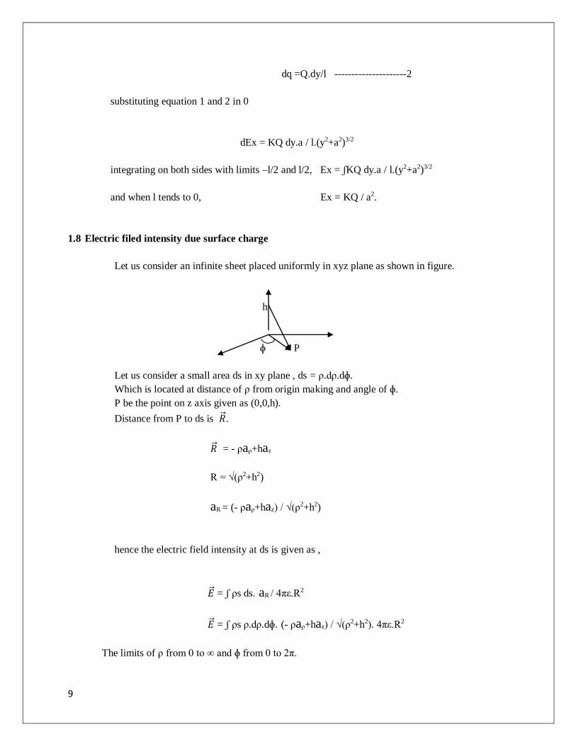
1.8 Electric filed intensity due surface charge
Let us consider an infinite sheet placed uniformly in xyz plane as shown in figure.
h
ɸ P
Let us consider a small area ds in xy plane , ds = ρ.dρ.dɸ.
Which is located at distance of ρ from origin making and angle of ɸ.
P be the point on z axis given as (0,0,h).
Distance from P to ds is �⃗� .
�⃗� = - ρaρ+haz
R = √(ρ2+h2)
aR = (- ρaρ+haz) / √(ρ2+h2)
hence the electric field intensity at ds is given as ,
�⃗� = ʃ ρs ds. aR / 4πε.R2
�⃗� = ʃ ρs ρ.dρ.dɸ. (- ρaρ+haz) / √(ρ2+h2). 4πε.R2
The limits of ρ from 0 to ∞ and ɸ from 0 to 2π.

10
�⃗� = ʃ ʃ ρs ρ.dρ.dɸ. (- ρaρ+haz) / √(ρ2+h2). 4πε.R2
By simplying above equation, the electric field intensity
�⃗� = ρs az / 2ε.
1.9 Work done in moving point charge
Let us consider a charge q is placed in the existing electric field . The charge q experiences force
𝐹⃗⃗ ⃗⃗ ⃗⃗ ⃗⃗ ⃗⃗ ⃗⃗ ⃗⃗ ⃗⃗ ⃗.
�⃗�
------------------------------
a -----------------------------b
------------------------------
Here charge q is made to move from a to b of length l through electric field intensity �⃗� .
dw = -𝐹 dl = -q�⃗� dl
integrating on both sides, w = -qʃ �⃗� dl with limits a to b.
1.10 Electric Potential
From the above discussion work done to move point charge through the existing electric field is
w = -qʃ �⃗� dl
but we know that electric potential is defined work done to move unit charge
V = w/q
Therefore, V = w/q = -ʃ �⃗� dl with limits a to b
V = -�⃗� l with limits a to b
Hence , electric potential V = Va - Vb
11
1.11 Electric potential due to point charge
P (point charge)
�⃗�
------------------------------
a -----------------------------b
------------------------------
Let the charge q is moved from a to b and at point charge is Q from ra and rb ,
We know that electric potential, V = q/(4πεr)
Electric field intensity at point p due to charge at a is, Va = Q/(4πεra)
Electric field intensity at point p due to charge at a is, Vb = Q/(4πεrb)
Hence potential difference or electric potential from a to b is,
Vab = Va - Vb
Vab = Q/(4πεra) - Q/(4πεrb)
Vab = Q(rb - ra)/(4πεrarb).
1.12 Electric Flux
Macheal faraday has conducted experiment on two concentric spheres, inner layer is
positively charges and outer layer negatively charge, then he observe that their some sort of
displacement from inner layer to outer layer , this displacement is pronounced as electric flux
between spheres.
1.13 Electric Flux Density
We know that electric field intensity is , E = (K q / r2)
= q/ (4πε r2)
D=ε E = q/ (4π r2)—electric flux density
Electric flux density is defined as charge per unit area.

12
Potential gradient: potential gradient is defined as electric change in electric potential due to change
in the distance or length.
E = - ▼V
Properties of Potential:
Potential is the energy acquired by the charge.
When charge travel from one end to other end in any element there is potential change from
high to low.
Potential acquired by point charge leads to electric field.
1.14 Gauss Law
Gauss law states that the total flux in the given surface is equal to charge enclosed in it.
ɸ = Q.
the total flux enlaced in given surface is
ɸ = ʃ E ds
= ʃ Q / (4πε r2) ds
= Q / (4πε r2). ʃ ds
= Q4π r2 / (4πε r2).
= Q / ε.
Applications of Gauss law
To apply gauss law first assume Gaussian surface.
The electric field intensity must be normal to the Gaussian surface.
Gaussian surface must be symmetry.
13
1.15 Maxwell First Equation
We know that electric flux passing through the surface is equal to 1/ ε times the net charge
enclosed.
ɸ = ʃs E ds = Q/ ε
ɸ = ʃs ε E ds = Q ε / ε
ɸ = ʃs D ds = Q
from the strokes theorem we can say that surface integral function is volume integral of divergence of
same function.
Q= ʃs D ds = ʃv (▼. D) dv ----------------------3
from the gauss law we can write , Q= ʃv ρv dv --------------------------- 4
by comparing equation 3 and 4
(▼. D) = ρv---------------------------5
Equation 3 and 5 are said to be Maxwell’s first and second equation.
1.16 Poission and Laplace Equations
From the Maxwell’s equation we know that,
(▼. D) = ρv-------------------------------------6
D = εE-------------------------- 7
Equation 7 in 6,
▼ εE = ρv
but we know that, E = - ▼V
▼ ε(-▼V) = ρv
▼2V = - ρv / ε ------------------8
14
Equation 8 is called poission’s equation.
In the uniform Gaussian surface ,
ρv = 0
Then equation 8 can be rewrite as,
▼2V = 0 ------------------9
Equation 9 is called as Laplace equation.

15
UNIT-II
ELECTRIC DIPOLE AND CAPACITANCE
16
2.1 Electric Dipole and Dipole Moment
Two opposite charges +q and –q separated by some distance d forms the electric dipole.
+q ----------------d--------------- -q
The distance travelled by the point charge is defined as dipole moment (or) the product of charge and
distance travelled by it is called as electric dipole.
P = qd ------------------------------------------------------------------ 1
Here , P electric dipole moment
d distance between opposite charges
the line between two charges is called as axis of dipole. Potential
2.2 Electric Dipole Potential
Let us assume two charges separated by distance d as shown in the figure
+q ----------------d--------------- -q
Here, O center of the axis between charges
P be the test point where potential is required.
OP with length of r.
AA1 perpendicular from A to OP.
BB1 perpendicular from A to OP.
∟POB = Ɵ
r >>> d
the line AP = A1P = OP + OA1--------------------------------2
from the right angle triangle AA1O, OA1 = OA cos Ɵ
17
hence equation 2 can be written as, AP = A1P = r + OA cos Ɵ
but, OA = d/2
AP = A1P = r + d/2 cos Ɵ
Hence the potential at P due negative charge at A is ,
VA = -Kq/ AP = -Kq/ r + d/2 cos Ɵ
Similarly from the right angle triangle BB1O, BP = B1P = r - d/2 cos Ɵ
Hence the potential at P due negative charge at A is ,
VB = Kq/ BP = Kq/ r - d/2 cos Ɵ
Therefore the total potential acting on P is , V = VA + VB
V = Kq[ (1/ r - d/2 cos Ɵ) - (1// r + d/2 cos Ɵ) ]
= Kqd.cos Ɵ/ (r2 – d2/4 cos2 Ɵ)
But we know that, r >>> d
V = Kqd.cos Ɵ/ r2
V = KP.cos Ɵ/ r2 , (P = qd) ----------------- 3
2.3 Electric Field Intensity due to Dipole
We know that electric field intensity in terms of electric potential is given as ,
E = - ▼V
From equation 3 we can say that potential due dipole is in spherical co-ordinates, therefore find
electric field intensity we shall use spherical co-ordinates.
▼V = -[ dv/dr + (1/r)dv/dƟ ]
Simplifying ▼V, dv/dr = -2KP.cos Ɵ/ r3

18
(1/r)dv/dƟ = -KP.sin Ɵ/ r3
Substituting above two equations in E, E = -[ (-2KP.cos Ɵ/ r3) + (- KP.sin Ɵ/ r3) ]
= [ (2KP.cos Ɵ/ r3) + ( KP.sin Ɵ/ r3) ]
= KP/ r3 [ (2cos Ɵ) + (sin Ɵ) ] ------------------- 4
2.4 Torque due to Electric Dipole
Let us consider two opposite charges are placed in the uniform electric field with their line of axis of
2r.
------------------------------
---------------Ɵ------------- E
------------------------------
------------------------------
The experienced by +q is , F1 = E.q
The experienced by -q is , F2= -E.q
The total experienced by the dipole is , F = F1 + F2
F = 0
But the due to force experienced by +q it tends to oscillate in the direction of E and –q in the
direction opposite to E, which leads torque of dipole.
T = magnitude of F x perpendicular distance
Between their line of action
T = E.q x 2r sinƟ
T = PE.sinƟ. ( q.2r = P)--------------5
+q
-q

19
2.5 Polarization
If an piece if dielectric or insulator placed between the charges plates of condenser, then center of
gravity of negative charges is concentrated towards positive plate and center of gravity of positives
charges concentrated towards negative plate, this process of separation opposite charges is called a
polarization.
Polarization is also defined as electric dipole moment per unit volume.
Let A be the area of cross section of dielectric,
l be the distance by with opposite charges are separated,
q total charge in the volume of dielectric
then polarization, P = dipole moment / volume
= q.l / A.l
= q / A ---------------------------------------------------------- 6
i.e the polarization numerically equal to surface charge density.
2.6 Dielectric Constant and Electric Susceptibilty
Dielectric constant is defined as ratio capacitance of capacitor with dielectric to the capacitance of
capacitor without dielectric .
Capacitance of capacitor with dielectric has low potential(Vd) than the capacitance of capacitor
without dielectric(V) .
K = V / Vd ------------------------------------------------------ 7
The polarization is directly proportional to the electric field intensity created between charges.
P α E
P = Ke E
Ke = P / E = electric susceptibility--------------------------- 8
20
2.7 Capacitor and its Capacitance
The basic capacitor element is formed by separated two parallel plates with some dielectric medium.
When some voltage is applied to such an element charge is formed between the plates, their by
capacitance of capacitor is defined as charge Q developed between the plates when voltage V is
applied.
C = Q / V ---------------------------------------------------- 9
The units of capacitance are Farads (F).
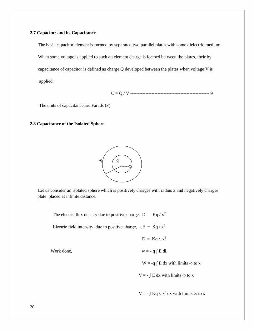
2.8 Capacitance of the Isolated Sphere
-q +q
∞ -----x—
Let us consider an isolated sphere which is positively charges with radius x and negatively charges
plate placed at infinite distance.
The electric flux density due to positive charge, D = Kq / x2
Electric field intensity due to positive charge, εE = Kq / x2
E = Kq /. x2
Work done, w = - q ʃ E dl.
W = -q ʃ E dx with limits ∞ to x
V = - ʃ E dx with limits ∞ to x
V = - ʃ Kq /. x2 dx with limits ∞ to x

21
= -K.q / (-. x ) with limits ∞ to x
= K.q / (. x )
But the capacitance is given charge per voltage, C = q / V
C = ( x ) / K ------------------------------- 10
2.9 Capacitance of the spherical Sphere
-q
+ + q
a
b
B
Let us consider an isolated sphere which is positively charges with radius a and negatively charges
plate placed at b distance.
The electric flux density due to positive charge, D = Kq / x2
Electric field intensity due to positive charge, εE = Kq / x2
E = Kq /. x2
Work done, w = - q ʃ E dl.
W = -q ʃ E dx with limits b to a
V = - ʃ E dx with limits b to a
V = - ʃ Kq /. x2 dx with limits b to a

22
= -K.q / (-. x ) with limits b to a
= 𝐾𝑞
. [ (1/a) – (1/b) ]
= 𝐾𝑞 (𝑏−𝑎)
ab
But the capacitance is given charge per voltage, C = q / V
C = ab / K(b-a) ------------------------------- 11
2.10 Capacitance of the Parallel Plates
+q - q
d
Let potential applied to these parallel plates is V their by forming charge q between them.
Electric flux density between plates, D = q / A
εE = q / A
E = q / ε.A,
V = E.d
V = q d / ε.A
But the capacitance is given charge per voltage, C = q / V
C = ε.A / d ------------------------------- 12
23
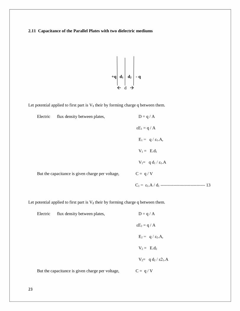
2.11 Capacitance of the Parallel Plates with two dielectric mediums
+q d1 d2 - q
d
Let potential applied to first part is V1 their by forming charge q between them.
Electric flux density between plates, D = q / A
εE1 = q / A
E1 = q / ε1.A,
V1 = E.d1
V1= q d1 / ε1.A
But the capacitance is given charge per voltage, C = q / V
C1 = ε1.A / d1 ------------------------------- 13
Let potential applied to first part is V2 their by forming charge q between them.
Electric flux density between plates, D = q / A
εE2 = q / A
E2 = q / ε2.A,
V2 = E.d2
V2= q d2 / ε21.A
But the capacitance is given charge per voltage, C = q / V

24
C2 = ε2.A / d2 ------------------------------- 14
Hence total capacitance between plates with multiple dielectric mediums is ,
C = C1 + C2
= (ε1.A / d1) + (ε2.A / d2)
= A / [ (d1/ ε1) + (d2/ ε2) ---------- 15.
2.12 Capacitance of the Co-axial Cable
Let us consider co-axial cable two isolated sphere with radius a and b from center of axis
b
a
the length of cable is , then line charge distribution ρl = q / l
the electric flux density generally in cable is , D = ρl / 2πr
therefore electric filed intensity , E = ρl / 2πrε
the electric potential of the cable is , V = -ʃ Edr , with limits b to a
= -ʃ (ρl / 2πrε) dr
= -(ρl / 2πε) ʃ dr/r
= -(ρl / 2πε) .ln(r)
By applying limits, V = -(ρl / 2πε) .[ln(a) – ln(b)]
V = (ρl / 2πε) .ln(b/a)
The capacitance of co-axial cable, C = ρl / V

25
C = 2πε / ln(b/a) ----------------------------------- 21
2.13 Energy Stored in the Capacitor
+q - q
V
By the definition capacitance between plates is , C = q /V
Electric potential, V = dw / dq
dw = V dq
dw = (q / C) dq
integrating on both sides, w = ʃ (q / C) dq
w = q2 / 2C (or) ---------------------------- 16
w = (CV) 2 / 2C
w = CV2 / 2 (or)--------------------------- 17
w = q2 / 2C
w = Vq / 2 ---------------------------------18
2.14 Energy Density in the Static Electric Field
Energy density of capacitor is defined energy stored per unit volume.
Wd = energy stored / volume
Wd = CV2 / 2/ Ad
Wd = εA V2/d / 2. Ad

26
Wd = ε V2/2d2
Wd = εE2/ 2
Wd = DE/ 2 ------------------------------------ 19
From equation 19 we can write,
dW / dV = DE/ 2
dW = (DE/ 2) dV
integrating on both sides, energy stored W = ʃv(DE/ 2) dV -------------------- 20
2.15 current
The flow of electrons from one end to other end constitutes current. The rate of change of
Charge is also defined as current.
i= q / t = dq / dt ------------------------------------------------- 22
the units of current is ampere.
Current Density
If charge is distributed in the given area, then current density is defined as current constituted
In given area.
J = i / A (A/mt2) ----------------------------------------------- 23
J = di / ds
di = J .ds
integrating on both sides, i = ʃ J .ds
Convection Current Density
Let us consider a material with volume of charges (ρV) moving with drift velocity (Vd) , then
27
Convection Current density is defined as product volume of charges moving with drift velocity.
J = ρV x Vd ---------------------------------------------------------------- 24.
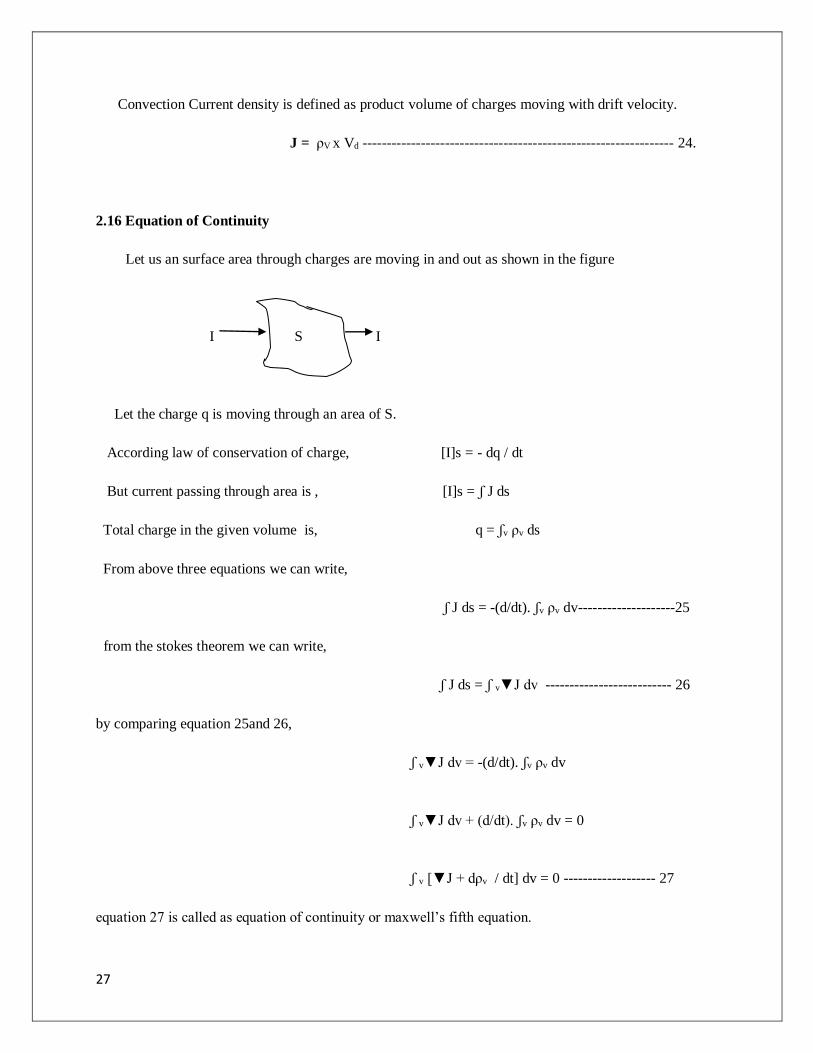
2.16 Equation of Continuity
Let us an surface area through charges are moving in and out as shown in the figure
I S I
Let the charge q is moving through an area of S.
According law of conservation of charge, [I]s = - dq / dt
But current passing through area is , [I]s = ʃ J ds
Total charge in the given volume is, q = ʃv ρv ds
From above three equations we can write,
ʃ J ds = -(d/dt). ʃv ρv dv--------------------25
from the stokes theorem we can write,
ʃ J ds = ʃ v▼J dv -------------------------- 26
by comparing equation 25and 26,
ʃ v▼J dv = -(d/dt). ʃv ρv dv
ʃ v▼J dv + (d/dt). ʃv ρv dv = 0
ʃ v [▼J + dρv / dt] dv = 0 ------------------- 27
equation 27 is called as equation of continuity or maxwell’s fifth equation.

28
UNIT-III
MAGNETO-STATICS
29
3.1 Introduction
Magneto-statics is the study of magnetic field developed by the constanr current through the coil
Or due to permanent magnets.
The behavior of contant magnetic field is studied by using two basic laws, they are
Bi-Savart’s law
Ampere’s circutal law.
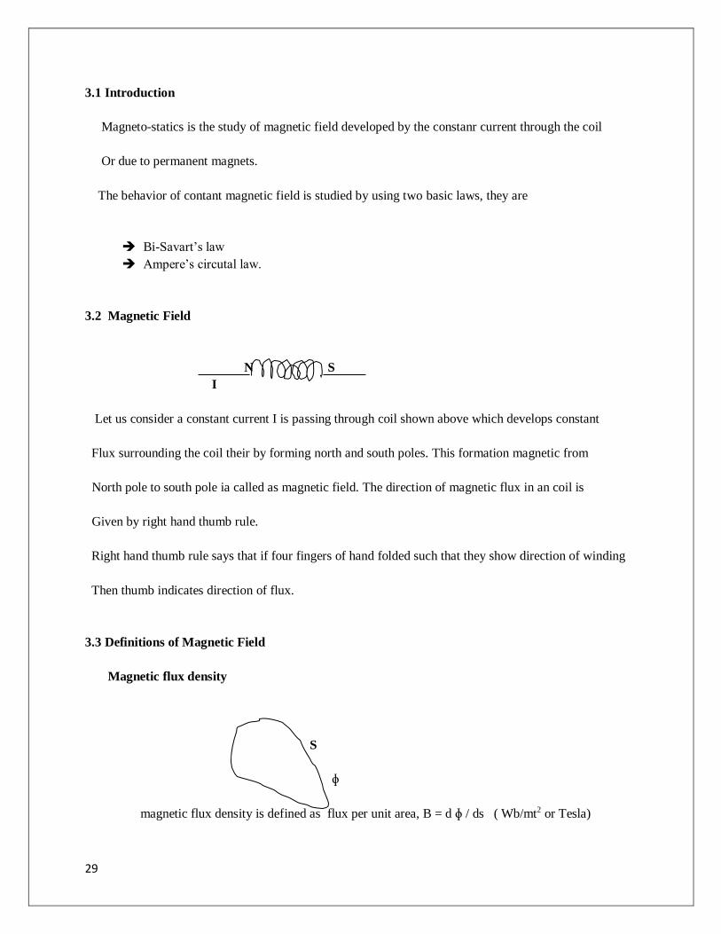
3.2 Magnetic Field
N S
I
Let us consider a constant current I is passing through coil shown above which develops constant
Flux surrounding the coil their by forming north and south poles. This formation magnetic from
North pole to south pole ia called as magnetic field. The direction of magnetic flux in an coil is
Given by right hand thumb rule.
Right hand thumb rule says that if four fingers of hand folded such that they show direction of winding
Then thumb indicates direction of flux.
3.3 Definitions of Magnetic Field
Magnetic flux density
S S
ɸ
magnetic flux density is defined as flux per unit area, B = d ɸ / ds ( Wb/mt2 or Tesla)
30
dɸ = B ds
by integrating on both sides we can determine total magnetic flux in area,
ɸ = ʃB ds -----------------------28
Magnetic Field Intensity
The force experienced by coil when some current passes through it is magnetic field
Intensity. Mathematically magnetic field intensity is givens as,
H = magnetic force / length
Magnetic force = NI
Length = l
Therefore magnetic field intensity, H = NI / l (AT/mt) ---------------------------- 29
Magnetic Permeabilty
Permeability is the inherent property of core which helps in sustaining flux in the core.
Mathematically permeability is given as, µ = B /H ------------------------- 30
From equation 30 the relation between flux density and intensity is ,
B = µ H ------------------------ 31
Where µ = µ0 µr
µ0 = absolute permeability = 4πx10-7 H/mt
µr = relative permeability
varies from core to core
Intensity of Magnetization
When a magnetic substance is placed in a magnetic field it experiences magnetic momentum.

31
The magnetic momentum per unit volume of substance is intensity of magnetization.
I = M / V
M = m.l ( m- pole strength of bar, l – length)
V = A.l
intensity of magnetization, I = m.l / A.l
I = m / A
Magnetic Susceptibility
The ratio intensity of magnetization to the magnetic field intensity is called as Magnetic
Susceptibility.
K = I / H.
Total flux density, B = B due to magnetic field + B due to intensity of magnetization of bar
B = µ0 H + I
But we know that, µ = B / H
= ( µ0 H + I ) / H
= µ0.+ (I/H)
µ0 µr = µ0.+ K
µr = 1 + K / µ0 ---------------------------------------------------------------- 31
µr > 1, paramagnetic materials
µr < 1, diamagnetic materials
µr = 0, non-magnetic materials

32
3.4 Biot-Savart’s Law
Bio and savart are two scientists who conducted experiments on current carrying conductor
To determine magnetic flux ddensity(B) at any point surrounding that conductor. Their
Conclusion is named as “Biot-Savart’s Law”.
P
B
Idl
I
Let us consider an conductor carrying current I, which develops magnetic flux density B surrounding
It. Here Idl is called as current element. To find total electric field intensity conductor is divided into
Number of current elements.
The magnetic field intensity due to current element Idl is dH at point P. According Bio-Savart’s law
dH α Idl (current element)
dH α sinƟ (angle between current element and length joining point)
dH α 1 / r2 (square of distance between current element and point)
by combining above three,
dH α Idl . sinƟ / r2
by removing proportionality,
dH = Idl . sinƟ / 4πr2
total magnetic field intensity at point P,
H = ʃ Idl . sinƟ / 4πr2
33
therefore total flux density at point P, B = µ H
B = µ ʃ Idl . sinƟ / 4πr2 -------------------------------------- 32
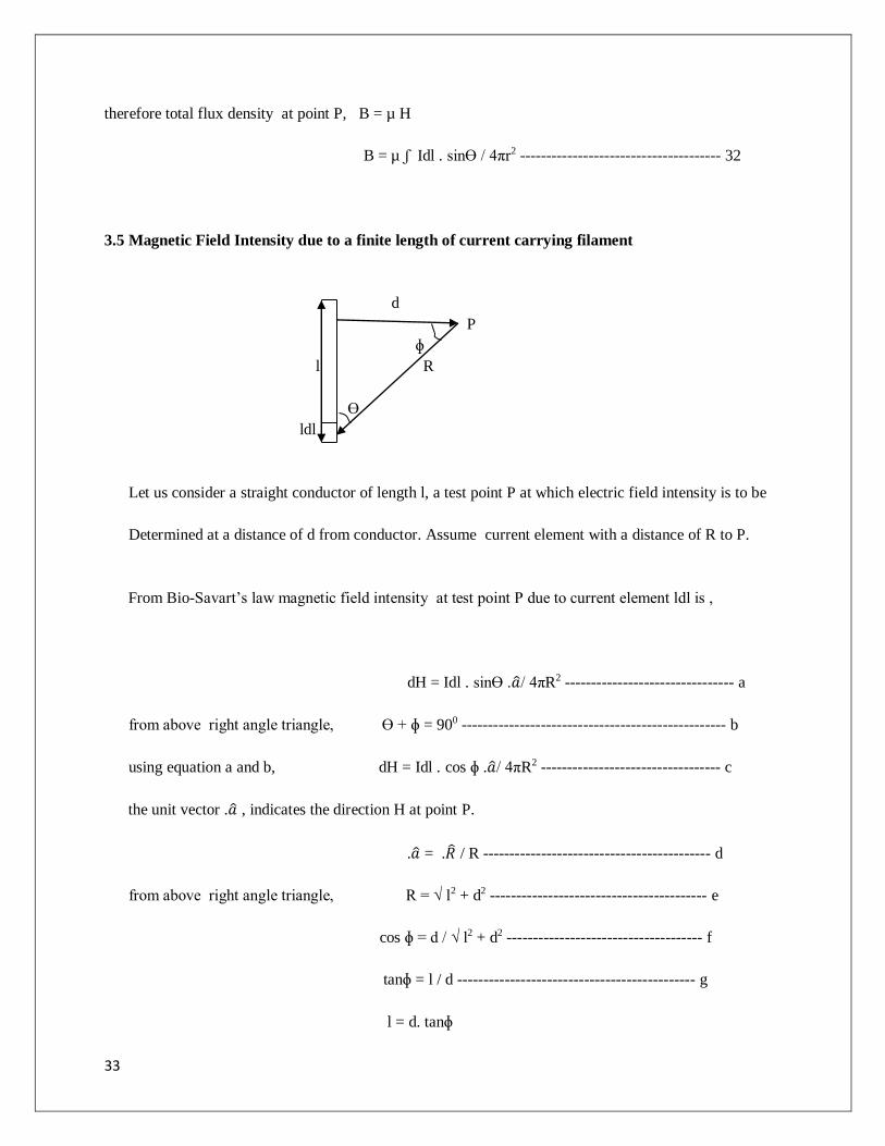
3.5 Magnetic Field Intensity due to a finite length of current carrying filament
d
P
ɸ
l R
Ɵ
ldl
Let us consider a straight conductor of length l, a test point P at which electric field intensity is to be
Determined at a distance of d from conductor. Assume current element with a distance of R to P.
From Bio-Savart’s law magnetic field intensity at test point P due to current element ldl is ,
dH = Idl . sinƟ .�̂�/ 4πR2 -------------------------------- a
from above right angle triangle, Ɵ + ɸ = 900 -------------------------------------------------- b
using equation a and b, dH = Idl . cos ɸ .�̂�/ 4πR2 ---------------------------------- c
the unit vector .�̂� , indicates the direction H at point P.
.�̂� = .�̂� / R ------------------------------------------- d
from above right angle triangle, R = √ l2 + d2 ----------------------------------------- e
cos ɸ = d / √ l2 + d2 ------------------------------------- f
tanɸ = l / d --------------------------------------------- g
l = d. tanɸ

34
dl = d sec2ɸ dɸ -------------------------------------- h
substituting d,e,f in c,
dH = Idl . cos ɸ .d .�̂�/ 4π (l2 + d2)2
integrating on both sides
H = ʃ Idl . cos ɸ .d .�̂�/ 4π (l2 + d2)3/2
H = 𝐼
4𝜋𝑑2 ʃ dl / (l2 / d2 + 1)3/2
H = 𝐼
4𝜋𝑑2 ʃ dl / (tan2ɸ + 1)3/2
Substituting equation h in above equation is ,
H = 𝐼
4𝜋𝑑2 ʃ d sec2ɸ dɸ / (sec2ɸ)3/2
H = 𝐼
4𝜋𝑑2 ʃ d sec2ɸ dɸ / (sec3ɸ)
H = 𝐼
4𝜋𝑑 ʃ cosɸ dɸ
H = 𝐼
4𝜋𝑑 sinɸ ---------------------------------------------------33
For straight line of infinite length, ɸ varies between –π /2 to π /2
Substituting above limits in equation 33, H = 𝐼
2𝜋𝑑 ---------------------------------------------------- 34
3.5 Magnetic Field Intensity due to a circular current carrying filament
Let us consider circular conductor with radius r,
Idl p r
r

35
magnetic field intensity at the center of circular conductor is,
from above figure we can say that idl and center are at 900
using Bio-Savart’s law magnetic field intensity at center point P due to current element ldl is,
dH = idl sin90 / 4πr2
dH = idl / 4πr2
integrating on both sides, H = ʃ idl / 4πr2
H = i ʃ dl / 4πr2 (ʃ dl = 2πr)
H = i 2πr / 4πr2
H = i / 2r ------------------------------------------------------- 34
Magnetic field intensity at the center of circular conductor with N number of turns is,
H = Ni / 2r ------------------------------------------------------- 35
3.6 Magnetic Field Intensity due to a Square current carrying filament
A B
a a
P
a a
D C
From the above figure we can say that each side AB,BC,CD,DA has magnetic field intensity at the center
Of square conductor.
In every right angle triangle angle between current element and center is 450.
The total magnetic field intensity at the center of square due to all corners using Bio-Savart’s law
Because of any one side, H = (I / 4πa) x[ sin450 + sin450 ]

36
Using all sides, H = 4(I / 4πa) x[ sin450 + sin450 ]
H = (I / πa) x[ 2 / √2 ]
H = (√2.I / πa) -------------------------------------36
3.7 Magnetic Field Intensity due to a Solenoid current carrying filament
The construction of solenoid is same as coil wounded on a cylinder , let us take take cylinder
As reference and derive expression for H due to solenoid. The solenoid with length l, number of turns
N allowing an current of I is shown in below figure,
dx
P
Assume a small length dx, with total turns ndx in it , let us derive what is the magnetic field intensity
Due to dx on P, their by total H at P.
A dx B
rdƟ c
r a a
dƟ
P Ɵ O
x
total number of turns = N
total length = l

37
number of turns per unit length, n = N / l
x be the distance of the point,
the magnetic field intensity due to length dx on P is ,
dH = (Ia2 / 2r3) ndx
from figure , r = √a2 + x2 , substituting r in dH.
dH = (Ia2 / 2 (a2 + x2)3/2) ndx
from above right angle triangles, dƟ<<<Ɵ, hence sin dƟ = dƟ
sin Ɵ = r dƟ / dx
sin Ɵ = a / r
substituting above deduction in dH,
dH = (Ia2 r.dƟ/ sin Ɵ / 2r3) n
dH = I.n. sin Ɵ. dƟ / 2 -------------------------------------------- a
if seen from end points of solenoid the magnetic field intensity at P is
P
Here from one end to other end angle varies from 0 to 2π, substituting above and integrating equation a
ʃ dH = ʃ I.n. sin Ɵ. dƟ / 2
H = - I.n.cos Ɵ. / 2, substituting above limits ----------------b
H = -(I.n/2) [cos2π – cos 0]
H = I.n = NI/l

38
if seen from end point of solenoid the magnetic field intensity at P at same end point,
then the limits varies between 0 to π/2
substituting above limits in b
H = -(I.n/2) [cosπ/2 – cos 0]
H = n.I/2 = N.I/ 2l ---------------------------------------------- 37
3.8 Maxwell’s Second Equation
From the guass law we can write magnetic flux in the given surface is surface integral of
Magnetic flux density.
Ψ = ʃ B.ds
But total flux density in closed surface is always zero,
Ψ = ʃ B.ds = 0
By applying divergence theorem we can write,
ʃ B.ds = ʃv▼ B.dv = 0
hence we can write , ▼ B = 0, is Maxwell’s second equation------------------------ 38
3.9 Ampere Circuital Law
The ampere circuital law states line integral magnetic filed intensity around any closed path
Is equal to total current enclosed in that path.
ʃ H dl = I -----------------------------------------------------------39
39
Ampere’s law is analogous to gauss law electro-statics.
Applications of Ampere’s law :
The magnetic field intensity in the surrounding closed path is always at tangential at
Each and every point on it.
At each every point on the closed path magnetic field intensity has the same value.
3.10 Maxwell’s Third Equation
From the ampere circuital law we know that,
ʃ H dl = I
but current can be written as, ʃ J ds = I
equating above two equations, ʃ H dl = ʃ J ds ---------------------------a
from stokes theorem, ʃ H dl = ʃ ▼x H ds --------------------- b
by combining equation a and b, ʃ ▼x H ds = ʃ J ds
by comparing on both sides, ▼x H = J , ▼x H = curl of H ------40
equation 40 is called as differential, integral or point form of ampere’s law and also called
as Maxwell’s Third Equation
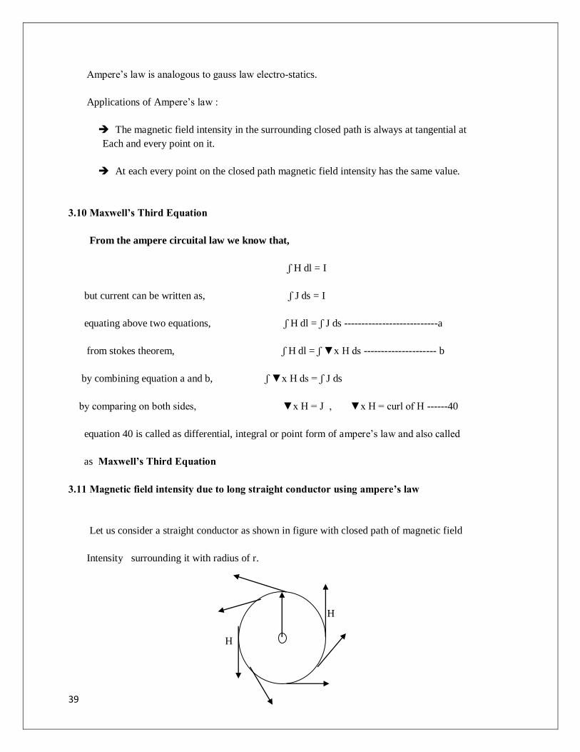
3.11 Magnetic field intensity due to long straight conductor using ampere’s law
Let us consider a straight conductor as shown in figure with closed path of magnetic field
Intensity surrounding it with radius of r.
H
H

40
From ampere’s circuital law we can write magnetic field intensity in closed path,
ʃ H dl = I -------------------------------------a
but we can write, ʃ H dl = H ʃ dl
= H 2πr ------------------------------ b
Equating a and b, H 2πr = I
H = I / 2πr ----------------------------------- 41
3.12 Magnetic field intensity due to infinite sheet conductor using ampere’s law
d
d d
d
let us consider a square sheet as shown above with surrounding current path of side d.
according to Ampere’s law ,
ʃ H dl = I
where ʃ dl indicates the mean length closed path,
ʃ dl = 4d
their by , H ʃ dl = I
H.4d = I
H = I/4d.----------------------------------------------------42
41
UNIT-IV
FORCE IN MAGNETIC FIELD AND MAGNETIC POTENTIAL
42
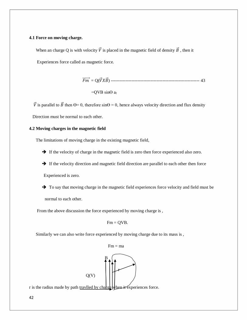
4.1 Force on moving charge.
When an charge Q is with velocity �⃗� is placed in the magnetic field of density �⃗� , then it
Experiences force called as magnetic force.
𝐹𝑚 ⃗⃗ ⃗⃗ ⃗⃗ ⃗ = Q(�⃗� 𝑋�⃗� ) ------------------------------------------------------------ 43
=QVB sinƟ af
�⃗� is parallel to �⃗� then Ɵ= 0, therefore sinƟ = 0, hence always velocity direction and flux density
Direction must be normal to each other.
4.2 Moving charges in the magnetic field
The limitations of moving charge in the existing magnetic field,
If the velocity of charge in the magnetic field is zero then force experienced also zero.
If the velocity direction and magnetic field direction are parallel to each other then force
Experienced is zero.
To say that moving charge in the magnetic field experiences force velocity and field must be
normal to each other.
From the above discussion the force experienced by moving charge is ,
Fm = QVB.
Similarly we can also write force experienced by moving charge due to its mass is ,
Fm = ma
B
r
Q(V)
r is the radius made by path travlled by charge when it experiences force.

43
Fm = mV2/r
By equating both forces, QVB = mV2/r
r = mV / QB
time taken to complete one revolution in field is ,
T = 2πr / V
= 2πm / QB
Hence frequency of charge in field is ,
F = 1/ T
= QB / 2πm, as this expression of frequency is independent
Of velocity it is called as cyclotron.
4.3 Lorentz force equation
We know that the force acquire by point charge when kept in the static electric field is,
𝐹𝑒⃗⃗ ⃗⃗ = Q �⃗�
The force experienced by moving charge in the magnetic field is ,
𝐹𝑚 ⃗⃗ ⃗⃗ ⃗⃗ ⃗ = Q(�⃗� 𝑋�⃗� )
The total force on the charge in the presence of both field is,
𝐹 = 𝐹𝑒⃗⃗ ⃗⃗ + 𝐹𝑚 ⃗⃗ ⃗⃗ ⃗⃗ ⃗
= Q �⃗� + Q(�⃗� 𝑋�⃗� )
44
= Q( �⃗� + (�⃗� 𝑋�⃗� )) -------------------------------------------------- 44
Equation 44 is called as Lorentz force equation.
4.4 Force on current element due to magnetic field
Let us a long conductor of length l which is partitioned into number parts allowing current
Of I. each part of conductor is of length dl, therefore individual part is represented with Idl called
As current element.
Force due to current element at any point
We know that convection current density is ,
𝐽 = ρv �⃗�
The current elements are ,
𝐽 dv = 𝐾 ds = 𝐼 dl
Using above two equations,
𝐼 dl = ρv �⃗� dv = Q�⃗�
Also current element, 𝐼 dl = (dQ/ dt).dl
= dQ. �⃗�
The force experienced by moving charge we know as ,
𝑑𝐹𝑚 ⃗⃗ ⃗⃗ ⃗⃗ ⃗⃗ ⃗⃗ = Q(�⃗� 𝑋�⃗� )
= 𝐼 dl X �⃗�
Integrating on both sides we can determine force due current element,
𝐹𝑚 ⃗⃗ ⃗⃗ ⃗⃗ ⃗ = ʃ 𝐼 dl X �⃗� ------------------------------------------ 45
Similarly, 𝐹𝑚 ⃗⃗ ⃗⃗ ⃗⃗ ⃗ = ʃs �⃗⃗� ds X �⃗�

45
𝐹𝑚 ⃗⃗ ⃗⃗ ⃗⃗ ⃗ = ʃv 𝐽 dv X �⃗�
4.5 Force on a straight long current carrying conductor placed in the magnetic field
B
l
Let us consider a straight conductor placed in the magnetic field as shown in the figure,
Of length l, allowing current of I, hence current element if Idl,
The velocity of charges in the given length of conductor is �⃗� .
The force experienced by current element is ,
𝑑𝐹𝑚 ⃗⃗ ⃗⃗ ⃗⃗ ⃗⃗ ⃗⃗ = dQ(�⃗� 𝑋�⃗� )
= dQ(dl/dt 𝑋�⃗� )
=I (𝑑𝑙⃗⃗ ⃗𝑋�⃗� )
Their by integrating on both sides, 𝐹𝑚 ⃗⃗ ⃗⃗ ⃗⃗ ⃗ = I (𝑙 𝑋�⃗� )
Fm = BIl sinƟ -------------------------------- 46
4.6 Force on a straight parallel long current carrying conductors placed in the magnetic field
P Q
I1 d I2

46
Let us consider two straight parallel current carrying conductors of length l separated by distance d
As shown above,
The magnetic field intensity due conductor P on Q is,
H = I1 / 2Πd
The magnetic flux density due conductor P on Q is,
B = µ0 I1 / 2Πd
Hence forced experienced by conductor Q due to field of P is,
F1 = B I2 l
= µ0 I1 I2 l / 2Πd
Similarly force experienced by P due to conductor Q is ,
F2 = µ0 I1 I2 l / 2Πd
Hence force per unit length of conductor is ,
(F / l) = µ0 I1 I2 / 2Πd ----------------------------------- 47
4.7 Magnetic dipole and dipole moment
Magnetic dipole is formed when two opposite magnetic charges are separated by distance l.
-Qm --------------l-------------- +Qm
The line joining two charges is termed as axis of dipole. Direction magnetic dipole is from -Qm to +Qm
In other words a bar magnet with pole strength Qm and l has , magnetic dipole moment, m =Qm l .
+Qm
47
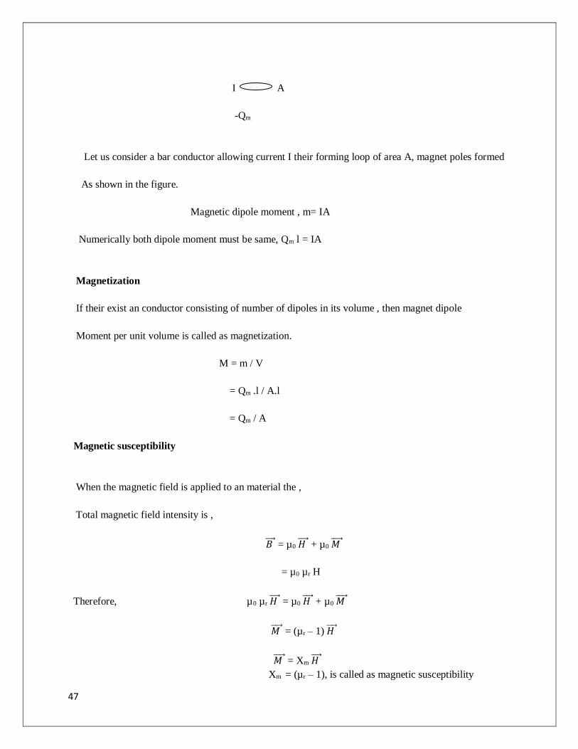
I A
-Qm
Let us consider a bar conductor allowing current I their forming loop of area A, magnet poles formed
As shown in the figure.
Magnetic dipole moment , m= IA
Numerically both dipole moment must be same, Qm l = IA
Magnetization
If their exist an conductor consisting of number of dipoles in its volume , then magnet dipole
Moment per unit volume is called as magnetization.
M = m / V
= Qm .l / A.l
= Qm / A
Magnetic susceptibility
When the magnetic field is applied to an material the ,
Total magnetic field intensity is ,
𝐵 ⃗⃗ ⃗ = µ0 𝐻 ⃗⃗⃗⃗ + µ0 𝑀 ⃗⃗⃗⃗
= µ0 µr H
Therefore, µ0 µr 𝐻 ⃗⃗⃗⃗ = µ0 𝐻 ⃗⃗⃗⃗ + µ0 𝑀 ⃗⃗⃗⃗
𝑀 ⃗⃗⃗⃗ = (µr – 1) 𝐻 ⃗⃗⃗⃗
𝑀 ⃗⃗⃗⃗ = Xm 𝐻 ⃗⃗⃗⃗
Xm = (µr – 1), is called as magnetic susceptibility

48
= 𝑀 ⃗⃗⃗⃗ / 𝐻 ⃗⃗⃗⃗ -------------------------------------- 48
4.7 Torque due to Magnetic dipole
Let us a sheet of side abcd placed in the magnetic field , the side ab experiences the force into
The page and side cd out of the page. Angles made by sheet with magnetic field are α and β.
Axis of rotation
d a
------------------------------------
------------------------------------
------------------------------------
------------------------------------
c b
d
the total torque experienced by sheet due to dipole is ,
T = 2 x torque on each side
= 2 x force x distance from axis of rotation
= 2 x F x d/2
= 2 x BIl cos β x d/2
= BIA cos β
= mB cos β or mB sin α
Therefore torque vector , �⃗� = �⃗⃗� x �⃗� -------------------------------------------------------- 49
4.8 Scalar magnetic potential

49
Form the electro-statics we know that, E = -▼V
Similarly in the magneto-statics , H = -▼Vm
Vm – vector magnetic potential
Applying curl on both sides of H, ▼x H = -▼x(▼Vm)
But curl of divergence of any vector is zero, ▼x H = 0
We can also write , ▼x H = J
From the above two equations we can write , J = 0.
This is possible only in the case constant magnetic field.
from the electro-statics we know that, ʃE dl = V
Similarly in the magneto-statics , ʃH dl = Vm
Ampere circuital law says that, ʃH dl = I
Comparing last two equations, Vm = I --------------------------------------------50
Hence the units of scalar magnetic potential is Amperes.
4.9 Vector magnetic potential
We know that divergence magnetic flux density over uniform closed surface is always zero.
▼B = 0
Also divergence of curl of vector is always zero.
▼ .(▼x A) = 0
By comparing above two equations,

50
B = ▼x A
µH = ▼x A
H = (▼x A) / µ
Applying curl on both sides,
▼x H = ▼x (▼x A) / µ = J
But, ▼x (▼x A) = ▼. (▼. A) - ▼2 A = µJ
For time invariant fields divergence of vector is zero, hence above can be written as
- ▼2 A = µJ
▼2 A = - µJ
Form the electro-statics we know that, dv = dq/ 4πε
Similarly in the magneto-statics , dA= µidl/ 4πr
Integrating on both sides, A = ʃ µidl/ 4πr, A- vector magnetic potential ---------51
4.10 Self inductance of a solenoid
d
i
let us consider a solenoid as shown in figure with length l allowing an current of i A.
N – total turns of solenoid coil
N – number of turns per unit length
51
magnetic filed density inside solenoid is , B = µ0 n.i.
total flux linking with coil is ɸ = N B A
= µ0 n l.i.A .n
= µ0 n2.i.A .l
Self inductance is the property of coil which is responsible for emf induced in it,
L = N ɸ / i
= µ0 n2.i.A .l / i
= µ0 N2A / l H ----------------------------52
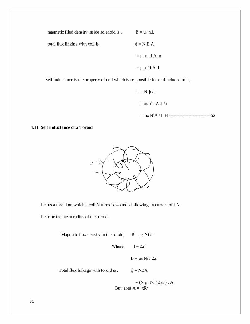
4.11 Self inductance of a Toroid
i r
Let us a toroid on which a coil N turns is wounded allowing an current of i A.
Let r be the mean radius of the toroid.
Magnetic flux density in the toroid, B = µ0 Ni / l
Where , l = 2πr
B = µ0 Ni / 2πr
Total flux linkage with toroid is , ɸ = NBA
= (N µ0 Ni / 2πr ) . A
But, area A = πR2
52
ɸ = ( N µ0 Ni / 2πr). πR2
= ( N2 µ0 i R2/ 2r).
Therefore self inductance of toroid is , L = ɸ / i
= ( N2 µ0 R2/ 2r). H ------------------------ 53
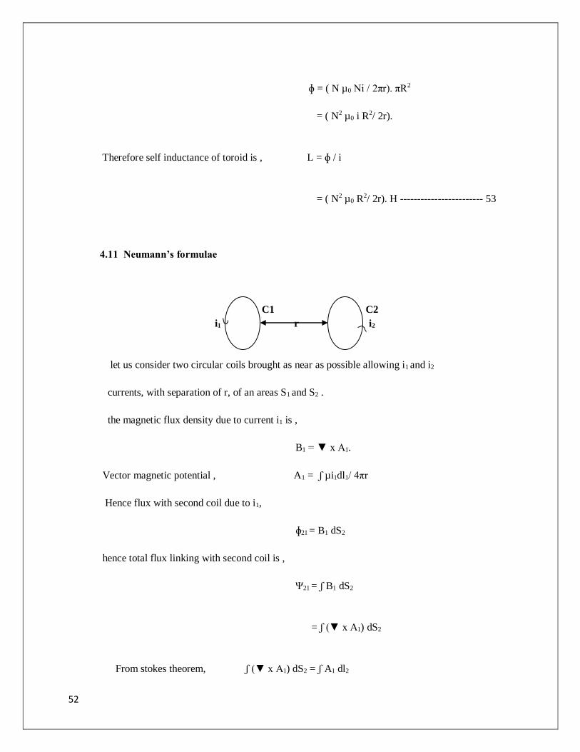
4.11 Neumann’s formulae
C1 C2
i1 r i2
let us consider two circular coils brought as near as possible allowing i1 and i2
currents, with separation of r, of an areas S1 and S2 .
the magnetic flux density due to current i1 is ,
B1 = ▼ x A1.
Vector magnetic potential , A1 = ʃ µi1dl1/ 4πr
Hence flux with second coil due to i1,
ɸ21 = B1 dS2
hence total flux linking with second coil is ,
Ψ21 = ʃ B1 dS2
= ʃ (▼ x A1) dS2
From stokes theorem, ʃ (▼ x A1) dS2 = ʃ A1 dl2

53
Substituting this inn above equation ,
Ψ21 = ʃ A1 dl2
= ʃ ʃ µi1dl1 dl2/ 4πr
Therefore mutual inductance between two coils is ,
M21 = Ψ21 / i1
Mutual inductance is the imaginary concept which says that there is flux linkage with second
Coil because of current flowing through first coil.
M21 = ʃ ʃ µi1dl1 dl2/ 4πr / i1
M21 = ʃ ʃ µdl1 dl2/ 4πr ------------- 54
This M21 is called as Neumann’s formulae.
4.11 Energy stored in the magnetic field
Let the work done to increase the current by di is dw, by law of conservation of energy
Work done is equal to energy stored .
dw = vi dt
= L.idi. dt/dt
dw = Lidi
integrating on both sides , ʃ dw = ʃ Lidi
w = Li2 / 2
but we know that, L = Nɸ / i = Ψ / i

54
using above expressions we can write energy stored in the magnetic field also as,
w = Ψ i / 2
= Ψ2 / 2 L. ------------------------------ 55
4.12 Mutual inductance between straight long and square conductors
Let us consider a straight and square conductor placed in the xy plane as shown.
y
i x b
d a d+a
here straight conductor is placed on y-axis and square loop as shown is xy plane.
The magnetic flux density due to straight wire o square loop is ,
B = µ0.i/ 2πx
The flux linking with square loop because current in straight wire is,
M = Ψ / I
From the gauss law we know that,
Ψ = ʃs B ds
= ʃ ʃ (µ0.i/ 2πx) dxdy, with limts
x = d to d+a, y = o to b
= ʃ (µ0.i/ 2πx).y dx
ds
55
Substituting limits of y, = ʃ (µ0.i/ 2πx).b dx
Then, = (µ0.i b / 2π).ln(x)
Substituting limits of x, = (µ0.i b ln(d+a)/ 2πln(d)).
Therefore mutual inductance between two conductors is ,
M = Ψ / i
= (µ0. B. ln(d+a)/ 2πln(d)).-------------- 56
4.13 Characteristics and applications of permanent magnets
Characteristics :
Permanent magnets are the one which readily available in nature in the form of
Bar and horse shoe shapes etc.
Permanent magnets irrespective of supply always exhibits magnetic properties.
Permanent magnets always develops a constant magnetic field.
The strength of the permanent magnets measured in terms of their cohesive force.
An permanent magnet with high cohesive force will have long life.
Permanent magnet got the disadvantage of ageing effect i.e in long run they may get rusted.
Applications:
Permanent magnets are used in the applications where ever it is required to develop
Constant magnetic field . Eg- Dc generator, Dc motor.

56
Horse shoe magnet Bar magnet

57
UNIT-V
TIME VARYING FIELDS AND NUMERICAL METHODS

58
5.1 introduction
Time varying fields are produced due to accelerated charges or time varying currents.
Here we shall study how time varying current affects electric and magnet fields.
5.2 Faraday’s law of electro-magnetic induction
Micheal faraday has stated two laws
i) If any coil experiences change in flux or variable flux then emf is induced in it.
ii) The emf induced in the coil is directly proportional to rate of change of flux linking
With the coil.
E α - dɸ / dt
E- electro-motive force.
- Sign indicates that magnetic flux developed in coil opposes the current through it.
From Lenz law.
For an coil with N turns emf induced in it ,
E = - N.dɸ / dt
5.3 Maxwell’s Fourth equation or vector form of faraday’s law
We know from the gauss law,
ɸ = ʃs B ds
hence emf induced due to above flux is ,
59
e = - dɸ / dt
= -d(ʃs B ds) /dt --------------------------a
Electric potential is given as ,
e = ʃ E dl --------------------------------------b
equating above two equations,
ʃ E dl = - (ʃs dB ds) /dt -------------------------- c
by applying stokes theorem,
ʃ E dl = ʃs (▼xE) ds
substituting above equation in c,
ʃs (▼xE) ds = - (ʃs dB ds) /dt
comparing on both sides,
▼xE = -dB/dt ---------------------------------------------- 57
Equation 57 is called as Maxwell’’s fourth equation of vector form of faraday’s law.
5.4 Types of induced emf
The emf induced in the coil according faraday’s law is mainly of two types. They are
i) Dynamically induced emf
ii) Statically induced emf.
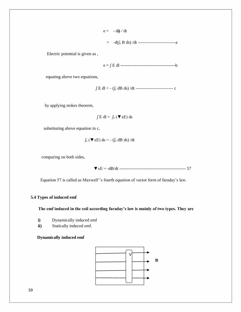
Dynamically induced emf
Vv B
V

60
Let us consider a straight conductor with charge velocity of v moving against the existing
Magnetic field. Force experienced by conductor is ,
𝐹 = Q ((�⃗� 𝑋�⃗� )
𝐹/Q⃗⃗⃗⃗⃗⃗ ⃗⃗ = ((�⃗� 𝑋�⃗� )
�⃗� = (�⃗� 𝑋�⃗� )
Hence electric potential induced in the conductor is ,
e = ʃ �⃗� dl
= ʃ (�⃗� 𝑋�⃗� ) dl
therefore potential induced can be written as, e = BVl sinƟ
the maximum value of potential induced is, e = BVl ---------------------------------- 58
Statically induced emf
If an conductor experiences variable flux then emf induced in it is called as statically induced
Emf.
e = ʃ �⃗� dl = -Ndɸ / dt
since the flux is alternating,
ɸ = ɸm sinwt
then the emf induced is ,

61
e = -Nd (ɸm sinwt ) / dt
= N ɸm w cos wt ------------------------------ 59
5.5 Displacement current
Let us consider a capacitor is connected to Ac source as shown in figure
V Q,C
The current flowing through capacitor is ,
iC = C dV / dt
the capacitance of capacitor,
C = ε A / d
Then, iC = (ε A / d). dV / dt
iC / A = ε dE / dt
Jc = dD / dt
Jc is called as displacement current.
V r C

62
Above is the figure of actual capacitor with internal resistance,
Then the total current is ,
i = ir + ic
where , I – total current
ir – current through resistance
ic – current through capacitance
dividing above KCL on both sides by area A,
i / A = ir / A + ic / A
J = Jr + Jc
Jr – conducting current
Jc – displacement current
5.6 Maxwell’s equations in time varying fields
In the time varying fields we can write,
E = Eo coswt
= Eo ejwt
Similarly, D = Do ejwt
d D / dt = Do wJ ejwt = Jw Do
likely, dB / dt = Jw B
we know that,
▼xE = - dB / dt

63
= Jw B
Also, ▼xE = -JwµH
▼x H= J+ dD/dt
= σE+ Jw Do
= σE+ Jw εE
= E (σ+ Jw ε)
Integak form,,
ʃ D ds = ʃ ρvdv
ʃ B ds = 0
ʃ E dl = - Jw ʃ B ds
ʃ H dl = (σ+ Jw ε) ʃ E ds
5.7 Numerical methods.
There are various numerical methods to calculate the electric filed intensity on a uniform
and non-uniform fields. They are
a) Finite difference method
b) Finite element method
c) Boundary element method
d) Charge simulation method.
Let us check short discussion of each method to calculate electric field intensity.
a) Finite difference method

64
2 1 p 3
4
h
Here let us consider an Uniform field whose electric field intensity is to be determined
The test area is portioned into number meshes as shown in the figure.
Each mesh is of step size h.
Each mesh can be studied with the knowledge of their four nodes.
With the knowledge of mesh field we can determine any unknown potential in the given field.
If P is the test point at field is to be determined , then the field function at P depends on Fields at neighboring nodes.
b) Finite element method
This method is applicable to both uniform and non-uniform test fields.
Let us consider a non-uniform field whose total field is to be determined.
Here total area of field is portioned into number known shapes like triangle, trapezoidal etc.
Each shape is pronounced as element.
Each element is described with corner nodes.
If the all node voltages of individual element is known then total potential of element
1 2
3 4

65
Can be determined.
Their by with all the element voltages we can calculate total electric field intensity of given
Medium.
c) Charge simulation method
Interface between electrode and dielectric
1 X 4 5
2 X Dielectric-1
X X
3 X
X 6
Dielectric -2
In this method we can find field due to point charges.
Here 1,2,3 -------6 are the point charges.
The x marks indicates counter points at which field is to be calculated.
Let us consider counter point 1 between electrode and dielectric -1 , hence the total potential
At this counter point is due to fields of point charges 1,2,4,5.
Similarly we can field at each counter point, their by total potential of interface is sum of
All counter point field.
This method has good accuracy and speed.
Can not be applicable for electrodes of irregular shapes
Accuracy in 2D is 1% and in 3D is 2%.
As point to point field is calculated , this can be easily simulated in the PC.
This method can be used for unbounded fields.
66
*** Boundary method is almost similar to charge simulation method , but here instead of point
Charges surface charges are considered. This method required large time and complexity increases.