Electricity Market Design An Agent-Based Computational

1

Agent-Based Computational Economics

A Constructive Approach to Economic Theory

Presenter:

Leigh Tesfatsion Professor of Econ, Math, and

Electrical & Computer Engineering

Iowa State University, Ames, Iowa 50011-1070

http://www.econ.iastate.edu/tesfatsi/

[email protected]

Last Revised: 2 December 2016

2

Outline

Complexity of Economic Processes

Agent-Based Computational Economics (ACE)

ACE Market Modeling: Examples 1. Double-Auction Market Model

2. Two-Sector Trading World (Hash & Beans)

3. Eurace: National Economy Modeling

4. Labor Market Networks Study

5. Trade Network Game (TNG)

6. Restructured Electricity Market Study

Potential Advantages/Disadvantages of ACE

3

ACE Resources

ACE Website www.econ.iastate.edu/tesfatsi/ace.htm

ACE Handbook (Tesfatsion & Judd, Handbooks

in Economics Series, North-Holland, 2006, 904pp)

www.econ.iastate.edu/tesfatsi/hbace.htm

4

5

Current ACE Research Areas (http://www.econ.iastate.edu/tesfatsi/aapplic.htm )

• Learning and embodied cognition

• Network formation

• Evolution of norms

• Real-world market studies (labor, energy, finance…)

• Industrial organisation

• Technological change and growth

• Macroeconomics

• Business and Management

• Automated markets and software agents

• Development of computational laboratories • Parallel experiments (real and computational agents)

• Empirical validation…and many more areas as well

6

Large numbers of economic agents involved in distributed local interactions

Two-way feedback between microstructure and macro regularities mediated by agent interactions

Potential for strategic behaviour

Pervasive behavioural uncertainty

Possible existence of multiple equilibria

Critical role of institutional arrangements

The Complexity of Economic Processes

7

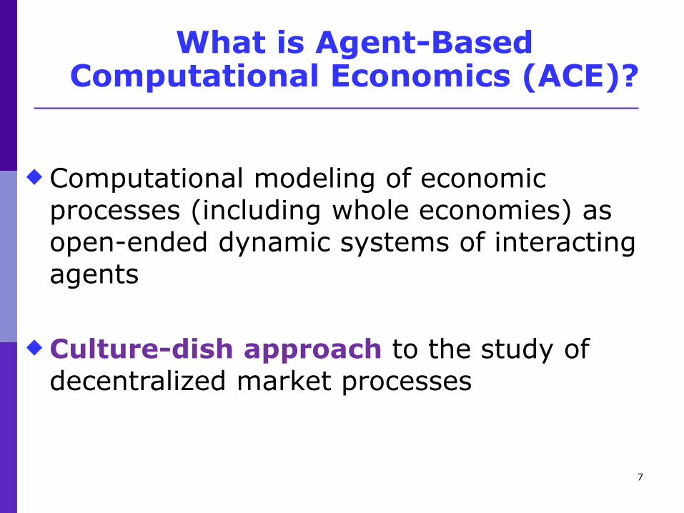
What is Agent-Based Computational Economics (ACE)?

Computational modeling of economic processes (including whole economies) as open-ended dynamic systems of interacting agents

Culture-dish approach to the study of decentralized market processes

8

ACE Modeling: Culture Dish Analogy

Modeler constructs a virtual economic world populated by various agent types (economic, institutional, social, biological, physical)

Modeler sets initial world conditions

Modeler then steps back to observe how the world develops over time (no further intervention by the modeler is permitted)

World events are driven by agent interactions

9

ACE culture dish analogy…

Initial World Conditions (Experimental Treatment Factors)

World Develops Over Time (Culture Dish of Agents)

Macro Regularities Micro to Macro Feedback Loop

Macro to Micro Feedback Loop

10

Key Characteristics of ACE Models

Agents are encapsulated software entities capable (in various degrees) of Adaptation to environmental conditions

Social communication with other agents

Goal-directed anticipatory learning

Autonomy (self-activation and self-determinism based on private internal processes)

Agents can be situated in realistically rendered problem environments

Behaviour and interaction patterns can develop/evolve over time

11

Four Main Strands of ACE Research

Empirical Understanding (possible reasons for observed regularities)

Normative Understanding (market design, fiscal/monetary policy design,…)

Qualitative Insight/Theory Generation (self-organization of decentralized markets,…)

Methodological Advancement (representation, visualization, validation,…)

12

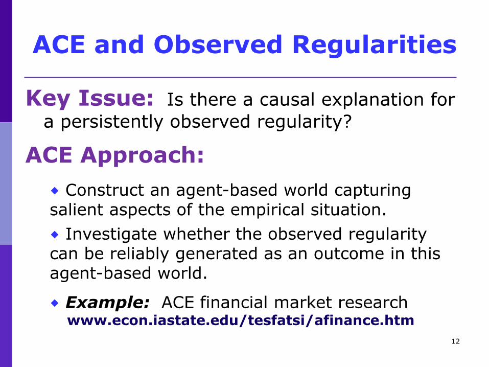
ACE and Observed Regularities

Key Issue: Is there a causal explanation for

a persistently observed regularity?

ACE Approach:

Construct an agent-based world capturing salient aspects of the empirical situation.

Investigate whether the observed regularity can be reliably generated as an outcome in this agent-based world.

Example: ACE financial market research www.econ.iastate.edu/tesfatsi/afinance.htm

13

ACE and Institutional Design

Key Issue: Does an actual/proposed policy or

institutional design ensure efficient, fair, and orderly outcomes over time despite attempts by participants to “game” the design for their personal advantage?

ACE Approach: Construct an agent-based world capturing salient

aspects of the policy or institutional design.

Introduce decision-making agents with learning capabilities and let the world evolve.

Observe and evaluate the resulting outcomes.

14

ACE and Qualitative Analysis

A Key Issue: What are the performance

capabilities of decentralized markets?

(Adam Smith, F. Hayek, ...)

ACE Approach: Construct an agent-based world qualitatively

capturing key aspects of decentralized market economies (circular flow, limited information, …)

Introduce self-interested traders with learning capabilities and let the world evolve. Observe the degree of coordination that results over time.

15

Example 1: Study of a Relatively Simple

Double-Auction Market Design

J. Nicolaisen, V. Petrov, and L. Tesfatsion,

IEEE Transactions on Evolutionary Computation, 5(5),

2001, pp. 504-523 (C++/MatLab)

www.econ.iastate.edu/tesfatsi/mpeieee.pdf

Key Issue Addressed:

Relative role of structure vs. learning

in determining the performance of a

double-auction design for a day-ahead

electricity market.

16

Double-Auction Electricity Market (Nicolaisen, Petrov, Tesfatsion, IEEE-TEC, Vol. 5, 2001)

World Constructed and Configured

Sellers submits supply offers (asks)

Buyers submit demand bids

Matched seller-buyer pairs trade

Sellers/buyers update their situations

17

Key Issue Addressed

Relative role of structure vs. learning in determining double-auction performance.

Sensitivity of market efficiency and market power outcomes to changes in market structure

RCON = Relative seller/buyer concentration

RCAP = Relative demand/supply capacity

Sensitivity of market efficiency and market power outcomes to trader learning representations: Reinforcement Learning (RL) vs. social mimicry via Genetic Algorithms (GAs).

18

Market Efficiency, Market Power, and Market Concentration

Market Efficiency: the degree to which market participants succeed in extracting maximum total net benefits from the market.

Market power: the degree to which a market participant can profitably influence prices away from competitive levels.

Market concentration: the degree to which the majority of market activity is performed by a minority of the market participants.

19

Activity Flow for the Double Auction (DA)

Init.

Sellers

Buyers

Traders

Submit

true

reservation

values

as

bids/asks

Traders

Matches

bids/asks

Competitive

equilibrium

outcomes

Auctioneer

COMPETITIVE EQUILIBRIUM BENCHMARK

CALCULATION (OFF-LINE)

Submit

strategic

bids/asks

Traders

Matches

bids/asks

Clearing

prices,

quantities

Auctioneer

Receive

auction results

Updating &

learning

Traders

End

Report

rounds runs

ACTUAL DOUBLE-AUCTION PROCESS

(DISCRIMINATORY-PRICE DOUBLE AUCTION WITH STRATEGIC BIDS/ASKS)

20

Activity Flow for the Double Auction (DA)

Init.

Sellers

Buyers

Traders

Submit

true

reservation

values

as

bids/asks

Traders

Matches

bids/asks

Competitive

equilibrium

outcomes

Auctioneer

COMPETITIVE EQUILIBRIUM

BENCHMARK CALCULATION (OFF-LINE)

Submit

strategic

bids/asks

Traders

Matches

bids/asks

Clearing

prices,

quantities

Auctioneer

Receive

auction results

Updating &

learning

Traders

End

Report

rounds runs

RUN-TIME AUCTION PROCESS

21

World Agent

Public Access:

// Public Methods The World Event Schedule, i.e., a system clock that permits inhabitants to time and synchronize activities (e.g., submission of asks/bids into the DA market); Protocols governing trader collusion; Protocols governing trader insolvency; Methods for receiving data; Methods for retrieving World data.

Private Access: // Private Methods

Methods for gathering, storing, and sending data; // Private Data World attributes (e.g., spatial configuration); World inhabitants (DA market, buyers, sellers); World inhabitants’ methods and data.

22

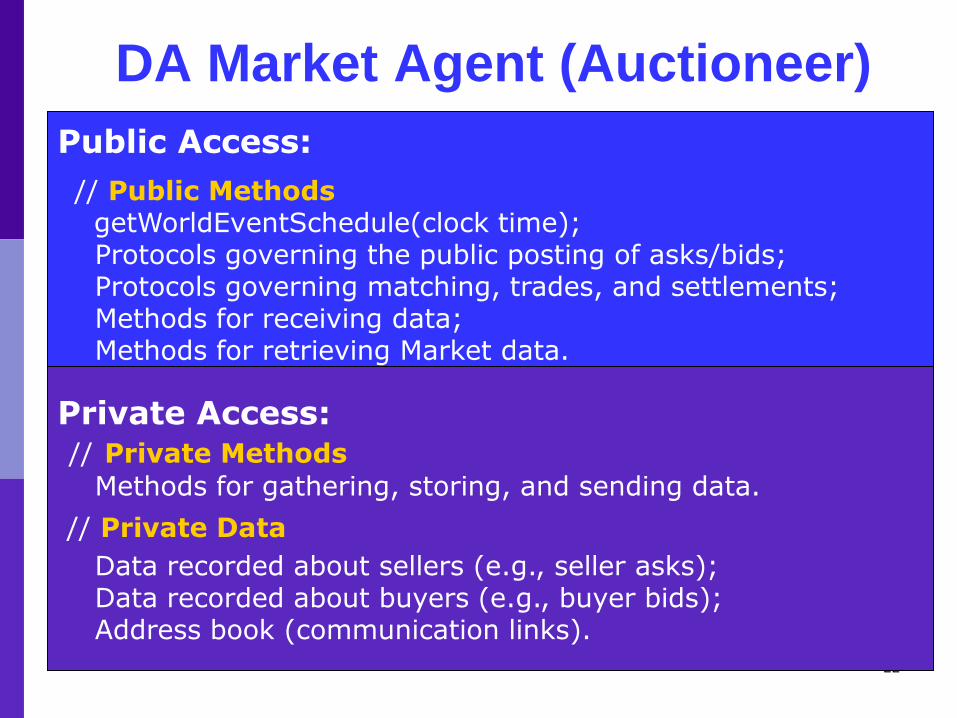
DA Market Agent (Auctioneer)

Public Access:

// Public Methods getWorldEventSchedule(clock time); Protocols governing the public posting of asks/bids; Protocols governing matching, trades, and settlements; Methods for receiving data; Methods for retrieving Market data.


Methods for gathering, storing, and sending data.

// Private Data

Data recorded about sellers (e.g., seller asks); Data recorded about buyers (e.g., buyer bids); Address book (communication links).

23

DA Trader Agent

Public Access:

// Public Methods getWorldEventSchedule(clock time); getWorldProtocols (collusion, insolvency);

getMarketProtocols (posting, matching, trade, settlement);

Methods for receiving data;

Methods for retrieving Trader data.


Method for calculating my expected profit assessments; Method for calculating my actual profit outcomes; Method for updating my ask/bid strategy (LEARNING). // Private Data Data about me (history, profit function, current wealth,…); Data about external world (rivals’ asks/bids, …); Address book (communication links).

24

Dynamic Flow of DA Market

World Constructed. World configures DA Market and Traders, and starts the clock.

Traders receive time signal and submit asks/bids to DA Market

DA Market matches sellers with buyers and posts matches

Traders receive posting, conduct trades, and calculate profits

Traders update their exp’s & trade strategies

25

Traders Learn to Select Asks/Bids (“Actions”) via Modified Roth-Erev RL

Action choice a leads to profits , followed by updating of action choice propensities q based on these profits, followed by transformation of these propensities into action choice probabilities Prob

Action Choice a1

Action Choice a2

Action Choice a3

Choice Propensity q1 Choice Probability Prob1

Choice Propensity q2

Choice Propensity q3

Choice Probability Prob2

Choice Probability Prob3

update choose transform

26

Roth-Erev Algorithm Outline

1. Initialize action propensities to an initial

propensity value.

2. Generate choice probabilities for all actions

using current propensities.

3. Choose an action according to the current

choice probability distribution.

4. Update propensities for all actions using the

reward (profits) for the last chosen action.

5. Repeat from step 2.

27

Structural Treatment Factor Values (Tested for Each Learning Treatment)

R C O N

RCAP

Ns = 3

Nb = 6

Cs = 10

Cb = 10

Ns = 3

Nb = 6

Cs = 20

Cb = 10

Ns = 3

Nb = 6

Cs = 40

Cb = 10

1/2

Ns = 3

Nb = 3

Cs = 10

Cb = 20

Ns = 3

Nb = 3

Cs = 10

Cb = 10

Ns = 3

Nb = 3

Cs = 20

Cb = 10

1

Ns = 6

Nb = 3

Cs = 10

Cb = 40

Ns = 6

Nb = 3

Cs = 10

Cb = 20

Ns = 6

Nb = 3

Cs = 10

Cb = 10

2

2 1 1/2

Ns = Number of Sellers

Nb = Number of Buyers

Cs = Seller Supply Capacity

Cb = Buyer Demand Capacity

28

Aggregate True Demand and Supply per Hour

Price ($/MWh)

Power (in MW=MWh per Hour)

37

16

35

17

12

11

10 20 40 60 80 120

Cell (3,1)

B 1,4

B 2,5

B 3,6

S 3

S 2

S 1 37

16

35

17

12

11

10 20 40 60

Price ($/MWh)

Power

Cell (3,2)

B 3,6

B 1,4

B 2,5

S 1

S 2

S 3

29

Summary of Policy-Relevant DA Findings

Market Efficiency: Generally high when traders use Roth-Erev individual reinforcement learning but not when traders use GA social mimicry (type of learning can matter).

Structural Market Power: Microstructure of the

DA market is strongly predictive for the relative

market power of traders (rule details matter).

Strategic Market Power: Traders are not able to change their relative market power through learning (importance of countervailing power).

30

Example 2: From Standard General Equilibrium to an ACE Trading World

Starting Point:

Two-Sector General Equilibrium (GE) Economy

Exercise:

• Remove all imposed equilibrium conditions (e.g., market clearing, correct expectations,...)

• Introduce minimal agent-driven production, pricing, and trade processes needed to re-establish complete circular flow among firms and consumers

• Experiment to see if/when resulting economy is able to attain an “equilibrium” state over time

31

Starting Point: Gen Equilibrium Hash & Beans Economy

B1

B3

B2

Bean Firms

H2

H1 H4

H3

Hash Firms

Consumer- Shareholders

Fictitious Auctioneer

pB,pH,DivB,DivH Demand(pB,pH,DivB,DivH)

pH

pB

SupplyB(pB),DivB SupplyH(pH),DivH

32

Plucking Out the Fictitious Auctioneer

B1

B3

B2

Bean Firms

H2

H1

H4 H3

Hash Firms

Consumer- Shareholders

Firm-Consumer Connections??

33

Plucking Out the Fictitious Auctioneer

Focus must now be procurement processes

Terms of Trade: Set production and price levels

Seller-Buyer Matching:

• Identify potential suppliers/customers

• Compare/evaluate opportunities

• Submit demand bids/supply offers

• Select suppliers/customers

• Negotiate supplier/customer contracts

Trade: Transactions carried out

Settlement: Payment processing and shake-out

Manage: Long-term supplier/customer relations

34

Illustration: ACE Hash-and-Beans (H&B) Economy

B1 B3

B2 B(0) Bean Firms

H2

H1 H4

H3

H(0) Hash Firms

Consumer-Shareholders

k=1,…,K(0)

Many- Seller Posted Bean Auction

Many- Seller Posted Hash Auction

SOB1

SOB2

SOB3

SOH1

SOH2

SOH3

SOH4

DivB DivH

Supply Offers

SO=(q,p)

35

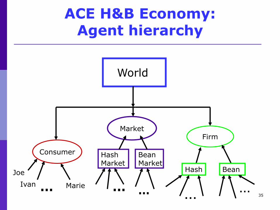
ACE H&B Economy: Agent hierarchy

World

Consumer

Firm

Hash Bean

Hash Market

Market

Bean Market

… … …

Joe

Ivan Marie … …

36

Overview of Activity Flow in the ACE H&B Economy

World agent constructed. World constructs & configures Market, Firm, & Consumer agents and starts a World “clock”.

Firms receive clock time signal and post quantities/prices in H & B markets

Consumers receive clock time signal and begin price discovery process

Firms/consumers match, trade, calculate profits/utilities, & update wealth levels

Firms and consumers update their expectations & behavioral strategies

loop

37

Each firm f starts out (T=0) with money Mf(0) and a production capacity Capf(0)

Firm f’s pro-rated sunk cost SCf(T) for T 0 is proportional to its current capacity Capf(T)

At beginning of each T 0, firm f selects a

supply offer = (production level, unit price)

At end of T 0, firm f is solvent if it has NetWorth(T)=[Profit(T) + Mf(T) + ValCapf(T)] > 0

If solvent, firm f allocates its profits (+ or -) between Mf, CAPf, & dividend payments.

Activity Flow for Firms

38

Each consumer k starts out (T=0) with a lifetime money endowment profile

( Mkyouth , Mkmiddle , Mkold ) In each T 0, consumer k’s utility is measured by

Uk(T)=(hash(T) - hk*)k • (beans(T) - bk*)[1-k]

In each T 0, consumer k seeks to secure maximum utility by searching for beans and hash to buy at lowest possible prices.

At end of each T 0, whether consumer k lives or dies depends on whether or not he secures at least his subsistence needs (bk*, hk*).

Activity Flow for Consumer-Shareholders

39

Initial number of consumers [ K(0) ]

Initial number/size of firms [ H(0), B(0), Capf(0)]

Firm learning (supply offers & profit allocations)

Firm cost functions

Firm initial money holdings [ Mf(0) ]

Firm rationing protocols (for excess demand)

Consumer learning (price discovery & demand bids)

Consumer money endowment profiles

(rich, poor, , , life cycle u-shape)

Consumer preferences ( values)

Consumer subsistence needs (b*,h*)

Experimental Design Treatment Factors

40

World Agent

Public Access:

// Public Methods The World Event Schedule, i.e., a system clock that permits inhabitants to time and synchronize activities (e.g., opening/closing of H & B markets); Protocols governing firm collusion; Protocols governing firm insolvency; Methods for receiving data; Methods for retrieving World data.


Methods for gathering, storing, and sending data; // Private Data World attributes (e.g., spatial configuration); World inhabitants (H & B markets, firms, consumers); World inhabitants’ methods and data.

41

Market Agent

Public Access:

// Public Methods getWorldEventSchedule(clock time); Protocols governing the public posting of supply offers; Protocols governing matching, trades, and settlements; Methods for receiving data; Methods for retrieving Market data.


Methods for gathering, storing, and sending data.

// Private Data

Data recorded about firms (e.g., supplies, sales); Data recorded about consumers (e.g., demands, purchases); Address book (communication links).

42

Consumer Agent

Public Access:

// Public Methods getWorldEventSchedule(clock time); getWorldProtocols (stock share ownership);

getMarketProtocols (price discovery process, trade process);


Methods for retrieving stored Consumer data.


Methods for gathering, storing, and sending data; Method for determining own budget constraint; Method for searching for lowest prices (LEARNING); Methods for changing my methods (LEARNING TO LEARN). // Private Data Data about self (history, utility function, current wealth,…); Data about external world (posted supply offers, …); Address book (communication links).

43

Firm Agent

Public Access:

// Public Methods getWorldEventSchedule(clock time); getWorldProtocols (collusion, insolvency);

getMarketProtocols (posting, matching, trade, settlement);


Methods for retrieving Firm data.


Methods for gathering, storing, and sending data; Methods for calculating own expected/actual profit outcomes; Method for allocating own profits to shareholders; Method for updating own supply offers (LEARNING); Methods for changing my methods (LEARNING TO LEARN). // Private Data Data about self (history, profit function, current wealth,…); Data about external world (rivals’ supply offers, demands,…); Address book (communication links).

44

Initial conditions carrying capacity?

(How many firms/consumers survive over long run?)

Initial conditions market clearing? (Supplies adequate to meet demands?)

Initial conditions market efficiency? (No wastage of physical resources or utility?)

Standard firm concentration measures at T=0

good predictors of long-run firm market power?

Importance for market performance of learning vs. market structure ? (Gode/Sunder, JPE, 1993)

Interesting Issues for Exploration

45

ACE Hash-and-Beans Economy Implementation (C. Cook, 2005, C#/.Net, Incomplete Project)

46

An Extended ACE Hash & Beans Economy

Marc Oeffner’s implementation of Agent Island (Thesis, 2008, Julius-Maximilians-Universitat Wurzburg )

Thesis/Code (SeSAm) Available At:

www.iastate.edu/tesfatsi/amulmark.htm

47

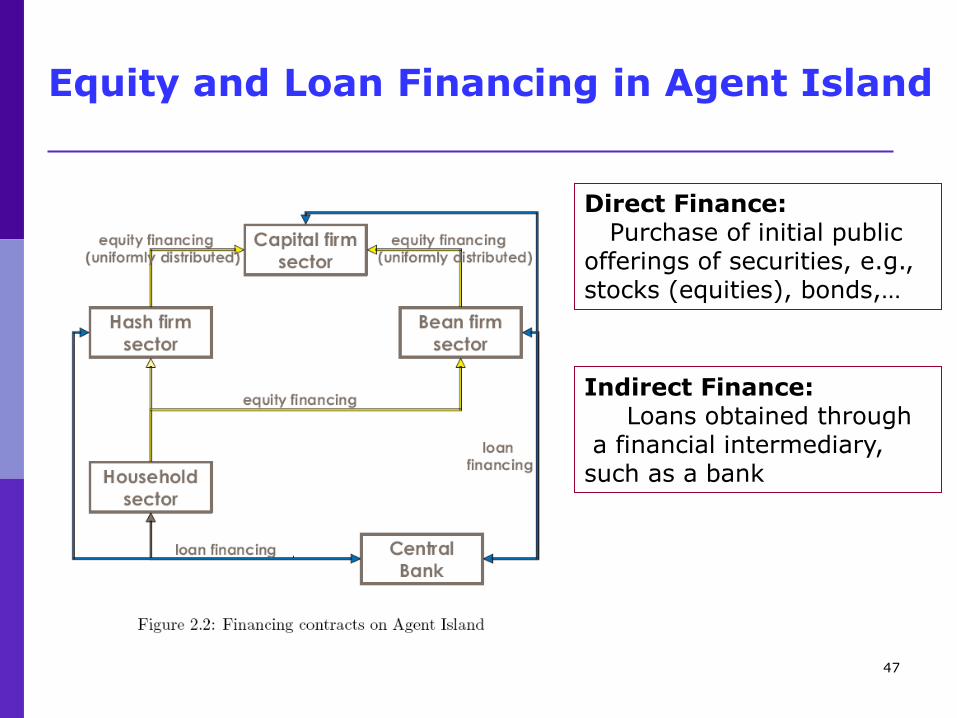
Equity and Loan Financing in Agent Island

Direct Finance: Purchase of initial public offerings of securities, e.g., stocks (equities), bonds,…

Indirect Finance: Loans obtained through a financial intermediary, such as a bank

48

Daily Activity Flow in Agent Island

49

Sample Outcomes for Agent Island

50

0 0

0 0

0 0

inflation

Real GDP

Investment demand

Period 1 (Shock Time) Period 2 (After Shock Time)

Sample PDFs for outcome changes due to a 1% increase in the credit interest rate occurring in period 1 and maintained in future periods

51

Example 3: EURACE -- Large-Scale ACE Model of the EU

52

53

54

Example 4: ACE Labor Market

Joint work with M. Pingle (U of Nevada-Reno)

Published in New Directions in Networks, 2003, Edward-Elgar volume, edited by A. Nagurney

M. Pingle and L. Tesfatsion, “Evolution of Worker-Employer Networks and Behaviors under Alternative Non-Employment Benefits: An Agent-Based Computational Economics Study”

Pre-print available at

www.econ.iastate.edu/tesfatsi/alabmplt.pdf

Parallel human-subject experiments conducted

55

ACE Labor Market Framework

W1 W2 W3 W12 . . .

E1 E2 E3 E12 . . .

Preferential job search with choice/refusal of partners: Red directed arrow indicates refused work offer.

56

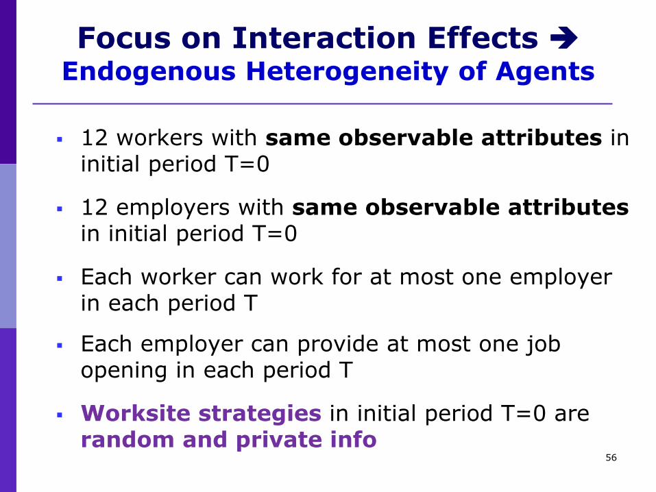
Focus on Interaction Effects Endogenous Heterogeneity of Agents

12 workers with same observable attributes in initial period T=0

12 employers with same observable attributes in initial period T=0

Each worker can work for at most one employer in each period T

Each employer can provide at most one job opening in each period T

Worksite strategies in initial period T=0 are random and private info

57

Publicly available information about various market/policy protocols, e.g., knowledge that each non-employed worker and vacant employer receives a Non-Employment Payment (NEP)

Private behavioral methods that can evolve over time

Privately stored data that can change over time

Each worker and employer has…

58

Worker Agent

Public Access:

// Public Methods Protocols governing job search; Protocols governing negotiations with potential employers; Protocols governing non-employment payments program; Methods for communicating with other agents; Methods for retrieving stored Worker data;

Private Access Only: // Private Methods

Method for calculating own expected utility assessments; Method for calculating own actual utility outcomes;

Method for updating own worksite strategy [ learning ]; // Private Data Data about own self (history, utility fct., current wealth…); Data recorded about external world (employer behaviors,…); Addresses for other agents [permits agent communication];

59

Employer Agent

Public Access:

// Public Methods Protocols governing search for workers; Protocols governing negotiations with potential workers; Protocols governing non-employment payments program; Methods for communicating with other agents; Methods for retrieving stored Employer data;

Private Access Only: // Private Methods

Method for calculating own expected profit assessments; Method for calculating own actual profit outcomes;

Method for updating own worksite strategy [ learning ]; // Private Data Data about own self (history, profit fct., current wealth…); Data recorded about external world (worker behaviors,…); Addresses for other agents [permits agent communication];

60

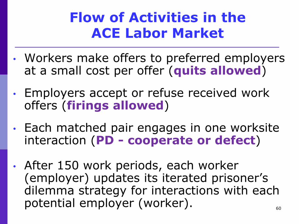
• Workers make offers to preferred employers at a small cost per offer (quits allowed)

• Employers accept or refuse received work offers (firings allowed)

• Each matched pair engages in one worksite interaction (PD - cooperate or defect)

• After 150 work periods, each worker (employer) updates its iterated prisoner’s dilemma strategy for interactions with each potential employer (worker).

Flow of Activities in the ACE Labor Market

61

x

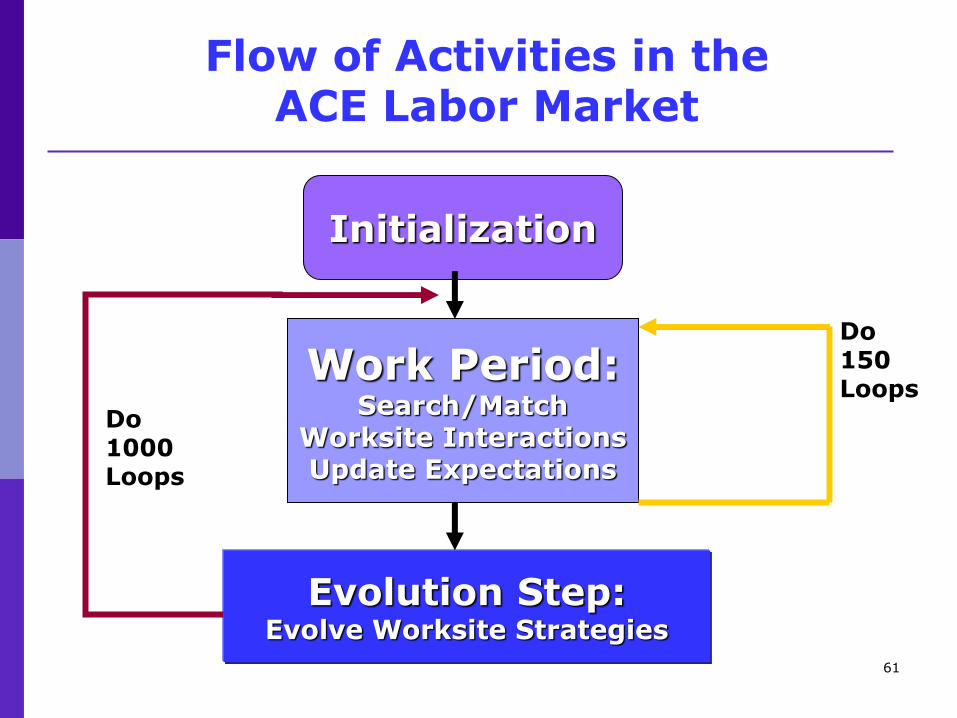
Flow of Activities in the ACE Labor Market

Initialization

Work Period: Search/Match

Worksite Interactions Update Expectations

Evolution Step: Evolve Worksite Strategies

Do 150 Loops

Do 1000 Loops

62

x

Worksite Interactions as Prisoner’s Dilemma (PD) Games

C

D

C D

Employer

Worker

(40,40) (10,60)

(60,10) (20,20)

D = Defect (Shirk); C = Cooperate (Fulfill Obligations)

63

Key Issues Addressed

How do changes in the level of the non-employment payment (NEP) affect...

• Worker-Employer Interaction Networks

• Worksite Behaviors: Degree to which workers/employers shirk (defect) or fulfill obligations (cooperate) on the worksite

• Market Efficiency (total surplus net of NEP program costs, unemployment/vacancy rates,...)

• Market Power (distribution of total net surplus)

64

Experimental Design

• Treatment Factor:

Non-Employment Payment (NEP)

• Three Tested Treatment Levels:

NEP=0, NEP=15, NEP=30

• Runs per Treatment:

20 (1 Run = 1000 Generations;

1 Gen.=150 Work Periods Plus Evolutionary Step)

• Data Collected Per Run: Network patterns,

behaviors, and market performance (reported

in detail for generations 12, 50, 1000)

65

Three NEP Treatments in Relation to PD Payoffs

NEP=0 < L=10

L=10 < NEP=15 < D=20

D=20 < NEP=30 < C=40

NOTE: Work-site PD payoffs given by: L (Sucker)=10 < D (Mutual-D) = 20 < C (Mutual-C) = 40 < H (Temptation) = 60

66

Market Efficiency Findings

As NEP level increases from 0 to 30…

• higher average unemployment and vacancy rates are observed; KNOWN EFFECT

• more work-site cooperation observed on average among workers & employers who match. NEW EX POST EFFECT

Note: These outcomes have potentially offsetting effects on market efficiency.

67

Efficiency Findings...

Market Efficiency (utility less NEP program costs) averaged across generations 12, 50, and 1000 for three different NEP treatments

NEP

Market Efficiency

0 15 30

88

90

60

68

Efficiency Findings...Continued

• NEP=15 yields highest efficiency

• NEP=0 yields lower efficiency

(too much shirking)

• NEP=30 yields lowest efficiency

(program costs too high)

69

Multiple Attractors

Two distinct “attractors” observed for each NEP treatment...

NEP=0 and NEP=15:

First Attractor = Latched network supporting mutual cooperation;

Second Attractor = Latched network supporting intermittent defection

NEP=30:

First Attractor = Latched network supporting mutual cooperation

Second Attractor = Disconnected network reflecting total coordination failure

70

The Following Diagrams Report...

Types of networks distinguished by “Network Distance” ND ranging across

ND=0 : Stochastic fully connected network

ND=12: Latched in pairs

ND=24: Completely disconnected

Types of worksite behaviors that are supported by these network outcomes

W W

E E

...

71

Network Distribution for NEP=0 Sampled at End of Generation 12

Network Distribution for ZeroT:12

0

2

4

6

8

10

12

14

16

18

20

1 2 3 4 5 6 7 8 9 10 11 12 13 14 15 16 17 18 19 20 21 22 23 24

Network Distance

Nu

mb

er

of

Ru

ns

Intermittent Defection Mutual Cooperation

ND

72



0

2

4

6

8

10

12

14

16

18

20

1 2 3 4 5 6 7 8 9 10 11 12 13 14 15 16 17 18 19 20 21 22 23 24

Network Distance

Nu

mb

er

of

Ru

ns


ND

73



0

2

4

6

8

10

12

14

16

18

20

1 2 3 4 5 6 7 8 9 10 11 12 13 14 15 16 17 18 19 20 21 22 23 24

Network Distance

Nu

mb

er

of

Ru

ns

Intermittant Defection Mutual Cooperation

ND

74


Network Distribution for LowT:12

0

2

4

6

8

10

12

14

16

18

20

1 2 3 4 5 6 7 8 9 10 11 12 13 14 15 16 17 18 19 20 21 22 23 24

Network Distance

Nu

mb

er

of

Ru

ns


ND

75



0

2

4

6

8

10

12

14

16

18

20

1 2 3 4 5 6 7 8 9 10 11 12 13 14 15 16 17 18 19 20 21 22 23 24

Network Distance

Nu

mb

er

of

Ru

ns


ND

76



0

2

4

6

8

10

12

14

16

18

20

1 2 3 4 5 6 7 8 9 10 11 12 13 14 15 16 17 18 19 20 21 22 23 24

Network Distance

Nu

mb

er

of

Ru

ns


ND

77


Network Distribution for HighT:12

0

2

4

6

8

10

12

14

16

18

20

0 1 2 3 4 5 6 7 8 9 10 11 12 13 14 15 16 17 18 19 20 21 22 23 24

Network Distance

Nu

mb

er

of

Ru

ns

Intermittent Defection Mutual Cooperation Coordination Failure

ND

78



0

2

4

6

8

10

12

14

16

18

20

0 1 2 3 4 5 6 7 8 9 10 11 12 13 14 15 16 17 18 19 20 21 22 23 24

Network Distance

Nu

mb

er

of

Ru

ns

Mutual Cooperation Coordination Failure

ND

79



0

2

4

6

8

10

12

14

16

18

20

0 1 2 3 4 5 6 7 8 9 10 11 12 13 14 15 16 17 18 19 20 21 22 23 24

Network Distance

Nu

mb

er

of

Ru

ns

Mutual Cooperation Coordination Failure

ND

80

Summary of Findings

• Changes in NEP have systematic effects on unemployment, vacancy, worksite behaviors, and welfare outcomes

• Worker-employer networks tend to be either fully latched in pairs (ND=12) or completely disconnected (ND=24)

• But… even fully latched networks (ND=12) can support multiple types of behavior across different runs ranging from full coop to mixed coop & defection

81

Evolution of trade networks among strategically interacting traders (buyers, sellers, dealers) with trades=PD games

Traders instantiated as tradebots (autonomous software entities) using TNG Lab

Event-driven communication among traders to determine their trade partners

Tradebots evolve trade strategies starting from initially random strategies

Tesfatsion(1996,1997); Mcfadzean/Tesfatsion(1999); McFadzean,Stewart,Tesfatsion (IEEE TEC, 2001)

Ex. 5: Trade Network Game (TNG)

www.econ.iastate.edu/tesfatsi/tnghome.htm

82

TNG Settings Screen

x

83

TNG Results Screen

X

x

84

TNG Chart Screen

x

85

TNG Network Animation Screen

x

86

TNG Network Physics Screen

x

87

Example 6: A Real-World Market Design Project

www.econ.iastate.edu/tesfatsi/AMESMarketHome.htm

AMES Market Package (Java):

An Open-Source Test Bed for the Agent-Based Modeling of Electricity Systems

Project Director:

Leigh Tesfatsion

Prof. of Econ, Math,& ECpE, Iowa State University

funded in part by

National Science Foundation, DOE at Pacific Northwest

National Lab, Sandia National Labs, and the

ISU Electric Power Research Center (EPRC)

88

Project Context

In April 2003, U.S. FERC proposed a Wholesale

Power Market Platform (WPMP) for common adoption by all U.S. wholesale power markets

Over 60% of electric power generating capacity in

the U.S. is now operating under some version of the WPMP market design

Basic Project Goal: Systematically examine dynamic performance of the WPMP market design as implemented in the U.S.

89

AMES Wholesale Power Market Test Bed (AMES = Agent-based Modeling of Electricity Systems)

Target Features of the AMES Test Bed Research/training grade model (2-500 pricing nodes)

Operational validity (structure, rules, behavioral

dispositions) Permits dynamic testing with learning traders Permits intensive sensitivity experiments

Open source (full access to implementation)

Easy modification (extensible/modular architecture)

Who should care? Academic researchers/teachers (understanding) Industry stakeholders (learn rules, test strategies) Policy makers (efficient and reliable market design)

90

Basic Project Approach:

Iterative Participatory Modeling

See, e.g., Barreteau et al. (JASSS 2003)

Stakeholders and researchers from multiple

disciplines join together in a repeated looping

through four stages of analysis:

Field work and data collection;

Role-playing games;

Agent-based model development (Java/RepastJ);

Intensive computational experiments.

91

Key Components of AMES Test Bed (Based on Business Practices Manuals for MISO/ISO-NE)

Two-settlement system

Day-ahead market (double auction, financial contracts)

Real-time market (settlement of differences)

AC transmission grid

Sellers/buyers located at various transmission nodes

Congestion managed via Locational Marginal Pricing (LMP)

Independent System Operator

System reliability assessments

Day-ahead bid/offer-based optimal power flow (OPF)

Real-time dispatch

Traders

Generators (Sellers)

LSEs (Buyers)

Follow market rules

Learning abilities

92

Example: 5-Bus Transmission Grid

A

B

C

E

D

Generator

Load

Transmission Line

Bus

93

AMES Framework: Agent Hierarchy

Traders

Buyers Sellers

Generators Load

Serving

Entities

ISO

Reliability

Commitment

Dispatch

Settlement

Real- Time

Re-Bid Period

Day- Ahead

FTR Bilateral

World

Transmission Grid Markets

94

Activities of AMES ISO During a Typical Day D-1

94

00:00

11:00

16:00

23:00

Real-Time

Market

(RTM)

open for

all 24

hours

hours of

day D-1

Day-Ahead Market (DAM)

for day D

ISO collects energy bids &

offers from LSEs & Generators

ISO solves SCED (bid/offer-based DC OPF) to determine

dispatch set-points & LMP schedule for all 24 hours

of day D.

ISO posts dispatch set-points and LMP schedule for each

hour of day D.

Day-ahead settlement

Real-time

settlement

95

Activity of AMES ISO on Successive Days D-1 and D

Morning of Day D-1 Afternoon of Day D-1 Thru

Operating Hour on Day D

ISO

Posting of

day-ahead

dispatch and

LMP

schedule

ISO

Dispatch

signals and

calculation

of real-time

LMPs

Adjust day-ahead

schedule

Reliability Assessment

Adjust

dispatch

set points .

DC OPF

Demand bids &

supply offers

submitted to the

day-ahead market

for day D .

ISO

96

Illustrative 5-Bus Test Case (Dynamic Extension of Static

ISO-NE/MISO/PJM Training Example)

G4

G2 G1 G3

G5

Bus 1 Bus 2 Bus 3

LSE 3 Bus 4 Bus 5

LSE 1 LSE 2

97

Illustrative 5-Bus Test Case…

G4

G2 G1 G3

G5

Bus 1 Bus 2 Bus 3

load

Bus 4 Bus 5

LSE 1 LSE 2

“Peaker” $$$

Cheap $

load load

LSE 3

Cheap $

$$

Cap 600

Cap 110

Cap 100

Cap 520

Cap 200

Thermal Limit

98

Daily LSE Load Profiles for 5-Bus Test Case

99

G4

G2 G1 G3

G5

Bus 1 Bus 2 Bus 3

LSE 3 Bus 4 Bus 5

LSE 1 LSE 2

Hour 17 Outcomes With No Generator Learning

(Generators report their true MC curves)

CONGESTED

G3 at upper

capacity limit 520

$

$ $

$$

$$$

110 100

600

200

Load=449 Load=385

Load=320

Limit=250

100

G4

G2 G1 G3

G5

Bus 1 Bus 2 Bus 3

Bus 4 Bus 5

LSE 1 LSE 2

Day 422-Hour 17 Outcomes With Gen Learning

(Each Generator i has converged with Prob(ai*) = 0.999)

$ $$$

$$ $ $

Load =449

Load=385

LSE 3 Load=320

Limit=250 CONGESTED

100

True Vs. Reported MC (Averaged)* on Day 422 (Each Generator i has converged with Prob(ai’) = 0.999)

Gen 2: True vs. Reported Average MC

5

15

25

35

45

55

65

75

0 100

Power Production Level

Marg

inal

Co

st

Reported MC

True MC


5

15

25

35

45

55

65

75

0 100


Marg

inal

Co

st

Reported MC

True MC


5

15

25

35

45

55

65

75

0 100


Marg

inal

Co

st

Reported MC

True MC


5

15

25

35

45

55

65

75

0 100


Marg

inal

Co

st

Reported MC

True MC

*NOTE: Reported marginal costs (MCs) for learning generators are 20-run

averages. Typical convergence time = 62 days, max time = 422 days. Omitted Gen 1 MC curve is similar to Gen 2’s.

102

ISO-Minimized Total Market Operation Costs (Day 422): No Learning Compared With Generator Learning

0

20,000

40,000

60,000

80,000

100,000

120,0000 2 4 6 8

10

12

14

16

18

20

22

Hour

Co

st

Gen Learning

No Learning

103

Five-Bus Test Case …

BOTTOM LINE:

Learning Matters !

104

AMES Software Development to Date

www.econ.iastate.edu/tesfatsi/AMESMarketHome.htm

Given supply behavior Learned strategic supply behavior

(Typical econ. lit. assumption) (Actual MISO/ISO-NE situation)‏

No trans./cap. constraints Transmission/capacity constraints


No market power mitigation ISO oversight & MP mitigation


Price-inelastic demand Demand bids with both fixed and

(Typical econ. lit. assumption) price-sensitive portions

(Actual MISO/ISO-NE situation)‏

No GUI capability GUI capability.

105

Potential Disadvantages of ACE

Intensive experimentation with relevant parameter

ranges needed to attain robust findings.

Experiments often result in outcome distributions rather than outcome point predictions.

Can be difficult to ensure results reflect aspects of the social/physical problem of interest and not simply the peculiarities of the programming implementation (hardware or software).

Creative modeling (rather than use of pre-existing frameworks) can require heavy investment of time and effort to acquire programming skills.

106

Potential Advantages of ACE

ACE facilitates empirical model validation since analytical tractability (requiring non-credible simplifications) is no longer an issue

ACE permits controlled study of systems involving complex interplay of structural, institutional, and behavioral aspects.

ACE test beds encourage creative experimentation. Researchers/students can evaluate interesting

conjectures of their own devising, with immediate feedback and no original programming required

Modular form of software permits relatively easy modification/extension of features.

Documents

Electricity Market Design An Agent-Based Computational