Embed Size (px)
Citation preview

UNIVERSITY OF CALGARY
Electrical Resistivity Ground Imaging (ERG!): Field Experiments to Develop
Methods for Investigating Fluvial Sediments
Christopher David Baines
A THESIS
SUBMITTED TO THE FACULTY OF GRADUATE STUDIES
IN PARTIAL FULFILLMENT OF THE REQUIREMENTS FOR THE
DEGREE OF MASTER OF SCIENCE
DEPARTMENT OF GEOGRAPHY
CALGARY, ALBERTA
AUGUST, 2001
O Christopher David Baines 2001

National Library Bibliotheque nationale du Canada
Acquisitions and Acquisitions et Bibliographic Sewices services bibliographiques
The author has granted a non- exclusive licence allowing the National Library of Canada to reproduce, loan, distribute or sell copies of this thesis in microform, paper or electronic formats.
The author retains ownership of the copyright in this thesis. Neither the thesis nor substantial extracts fiom it may be printed or otherwise reproduced without the author's permission.
L'auteur a accorde une licence non exclusive permettant a la Bibliothixpe nationale du Canada de reproduire, preter, distribuer ou vendre des copies de cette these sous la forme de rnicrofiche/film, de reproduction sur papier ou sur format electronique.
L'auteur conserve la propriete du droit d'auteur qui protege cette these. Ni la these ni des extraits substantiels de celle-ci ne doivent &re imprids ou autrement reproduits sans son autorisation.
Abstract
This research tested a new geophysical tool, electrical resistivity ground
imaging (ERGI). to map lithology and geometry of buried fluvial deposits. ERG1
uses measurements of the resistance of the ground to an electrical current to
develop a 2D model of the shallow subsurface (400 m).
Research was conducted in spring 2001 on an anastornosing reach of the
upper Columbia River, in southeastern B.C., Canada and in late summer 2001
on the Rhine-Meuse Delta, the Netherlands.
ERG1 surveys from 2 channel-fills and 2 crevasse-splays are presented
and corn pared to lithostratigraphic profiles from sediment cores. Depth, width and
lithology of sand channel-fills, crevasse-splays, and adjacent sediments can be
accurately detected and delineated from the ERG1 profiles, even when buried
beneath 1-20 rn of siltlclay.
Methodology experiments examined combined open water and dry land
ERG1 surveys, assessed electrode arrays, and identified a previously unreported
methodological problem: 'cumulative electrode charge-up'.
iii
. . Approval Page ................................................................................................................ 11 ... Abstract .................... .,.. .................................................................................................... 111
Table of Contents .................................... .... ................................................................. iv List of Tables ..................................................................................................................... vi . . List of Figures ................................................................................................................... v11
CHAPTER 1 . INTRODUCTION .................................................................................... 1
CHAPTER 2 . PREVIOUS RESEARCH ........................................................................ 3 2.1.1. Electrical Resistivity Ground Imaging .............................................. 3 2.1.2. Anastornosing River Deposits .................. .. .................................... 4
CHAPTER 3 . STUDY SITES .......................................................................................... 6 3- 1 . Upper Columbia River. British Columbia ............. .. ................ .. ............ 7
3.1. I . Regional Setting and Character ........................ .... ..................... 7 3.1.2. Survey Locations .............................................................................. 8
...................................................... 3 .2 . The Rhine-Meuse Delta. the Netherlands 10 3 .2.1. Regional Setting and Character ...................................................... 10 3.2.2. Survey Locations ...................... .... ....... ....,. . 11
CHAPTER 4 . ERG1 THEORY ..................................................................................... 13 ...................................................................................... 4.1 . Electrical Resistivity 13
4.2. Measuring Electrical Resistivity ...................~................................................ 16 4.3. Ground Imaging with Electrical Resistivity .............................................. 21 4.4. ERG1 Profile Confirmation and Ancillary Data .......................................... 23
................................................................................. CHAPTER 5. METHODOLOGY 24 .................................................................................. 5.1. ERG1 Data Acquisition 24
5.2. ERG1 Data Inversion ............................. .. ........................ 26 5.3. ERG1 Profile ConfirmationlAssessment ....................................................... 26 5.4. Locational Data Acquisition ........................................................................ 27
. 3 .5 Topographic Data Acquisition ............... ...,... .............................................. 27
CHAPTER 6. IMAGING FIELD EXPERLMENTS. ................................................... 28 6.1. Chame!-FiLI Imaging Field Experiment ..................................................... 28
6.1 -1 . Methods for this Field Experiment .............................................. 28 6.1 .2 . Results/Discussion ................... ....... . ....... ............................. 29
6.2. C revasse-S play lmaging Field Experiment .............................. .. ............. 34 6.2.1 . Methods for this Field Experiment ................................................. 35 6.2.2. Results/Discussion .......................................................................... 36

CHAPTER 7 . METHODOLOGY FIELD EXPERIMENTS ..................................... 45 7.1. Combination Land and Water ERG1 S w e y Field Experiment .................... 45
7.1.1. Methods for this Field Experiment ........................................... 4 6 7 . L .2 . Results/Discussion ................... .., ................................................ 48
7.2. Electrode Array Field Experiment ................................................................. 59 7.2.1. Methods for this Field Experiment ................................................. 60
............................................... 7.2.2. Results/Discussion ................... .... 61 7.3. Cumulative Electrode Charge-Up Effect Field Experiment .......................... 66
7.3.1 . Methods for this Field Experiment ................................................. 67 ........................................................................ 7.3.2. Results/Discussion 70
CHAPTER 8. CONCLUSIONS ..................................................................................... 76
REFERENCES ................................................................................................................ 78
APPENDIX A . GUIDELINES FOR ERG1 SURVEYING ......................................... 84 A . 1 ERG1 Site Selection .............................. .. ..................................................... 84 A.2 ERG1 Resolution and Depth of Investigation ................................................ 86 A.3 ERG1 Data Improvement ................................................................. .... .......... 87 A.4 Electrical Contact Resistance ............................. ,. ....................................... 89
................................................................................ A.5 Error Codes on the Sting 91 A.5 . 1 The HVOVL Error Code ...................... .. ........ .... 92 A.5.2 The TXOVL Error Code ........................................................... 93
.................................................................. A.5 -3 The NOVL Error Code 93 A.6 General Improvements to ERG1 Field Operations ......................................... 93 A.7 ERG1 Data Processing ................................................................................... 95
............................................................................... A.8 AGI's Command Creator 96 A.9 'Roll-Along' Surveying for ERG1 ..... .. ......................................................... 97
APPENDIX B . UNDERSTANDNG ELECTRODE ARRAYS FOR ERGI SURVEYS ........................................................................................................................ 99
APPENDIX C . THE ERG1 12 STEPS ...................................................................... 101
APPENDIX D . COORDLYATES FOR ALL OF TKE DATA PRESENTED IN THE ............................................................... ..................... BODY OF THE THESIS .., 102
APPENDIX E . THETA-DATA AND PSEUDOSECTIONS ...................................... 104 E . 1 Data fiom the Upper Columbia River. British Columbia ......................... .... 105
E . 1.1 Beavertail Channel-Fill and Area, B.C ...................................... 106 E . 1.2 Beavertail Crevasse-Splay, B.C. ................................................. 1 10 E . 1.3 Herron Meadow Crevasse.Splay, B.C ........................................... 1 12
E.2 Data fiom the Rhine-Meuse Delta, the Netherlands .................................... 1 13 E.2.1 Schoonrewoerd Channel-Fill, the Netherlands .............................. 1 15 E.Z.2 Unnamed Channel-Fills by the Lek River, the Netherlands .......... 1 17

List of Tables
Table 1 UTM Coordinates for data from the upper Columbia River, B.C. ......... 102
Table 2 NLRD coordinates for data from the Rhine-Meuse Delta, the Netherlands. .............................................................................................. 103
Table 3 Location, survey series, survey number, survey goal, and cross- reference thesis section number for data from the upper Columbia River, B.C. ........................................................................................................... 105
Table 4 Metadata for ERG1 surveys on the Beavertail channel-fill and area. In this table, the Wenner electrode array is represented by the symbol 'W' and the dipole-dipole array is represented by the symbol 'D'. ......................... 107
Table 5 Meta-data for ERG1 surveys BTS2 and BTS4 on the Beavertail Crevasse-splay. In this table, the Wenner electrode array is represented by the symbol 'W'. .......................................................................................... 1 10
Table 6 Meta-data for the ERG1 surveys on the Herron Meadow crevasse-splay. In this table, the Wenner electrode array is represented by the symbol 'W' .................................................................................................................. 112
Table 3 Location, survey series, survey number, survey goal, and cross- reference thesis section number for data from the Rhine-Meuse Delta, the Netherlands. .............................................................................................. 1 14
Table 7 Meta-data for ERG1 surveys on the Schoonrewoerd channel-fill. In this table, the Wenner electrode array is represented by the symbol 'W' and the dipole-dipole array is represented by the symbol 'D'. ................................ I f 5
Table 8 Meta-data for ERG1 surveys at the study site adjacent to the Lek River. In this table, the Wenner electrode array is represented by the symbol 'W' and the Wenner-Schlumberger array is represented by the symbol 'S'. .... 1 17

List of Figures
Figure 1 A global view of the ERG1 study sites on the upper Columbia River, ................ British Columbia and on the Rhine-Meuse Delta, the Netherlands 6
Figure 2 Location of the ERG1 study area on the upper Columbia River, British Columbia. The exact locations of all the ERG1 surveys and lithostratigraphic logs on the upper Columbia River are provided in Appendix D. .................... 9
Figure 3 Location of the ERG1 study area in the Rhine-Meuse Delta, the Netherlands. The exact locations for all the surveys in the Rhine-Meuse Delta are included in Appendix D. ............................................................... 12
Figure 4 A block of homogenous material (shown in blue) with a given length (L) and area (A) will resist an electrical current (as provided by a direct current source such as a battery) in direct proportion to the electrical resistivity (p) of the material .................................................................................................. 14
Figure 5 Electrical resistivity measurements in the field use four electrodes inserted into the ground. Two of the electrodes, A and 6, inject current into the ground. The other two electrodes, M and N, are used to measure voltage drop across the surface of the ground. ...................................................... 16
Figure 6 Changing the location of an electrode array, without changing the distance between the electrodes, changes the location of the region of investigation for the resistivity measurement. The depth of the region of investigation does not change. The region of investigation is represented here as an over-simplified sharp-edged round two-dimensional area. In reality, the region of investigation is diffuse, amorphous, and three
................................................................................................ dimensional. 18
Figure 7 Changing the distance between the electrodes in an electrode array, without changing the location of the center of the array, changes the depth of the region of investigation for the resistivity measurement. The horizontal location of the region of investigation does not change. Note that increasing the distance between the electrodes increases the size of the region of investigation in all directions. This increase in size vastly increases the volume of material contributing to the resistivity measurement. .................. 20
Figure 8 A diagrammatic representation of a multielectrode resistivity system used for ERG1 surveys. ............................................................................... 21

Figure 9 Comparison between an inverted resistivity block model and a contoured model. The block model more closely represents the mathematical output of the inversion process, while the contoured model is
....................................................................................... easier to interpret 22
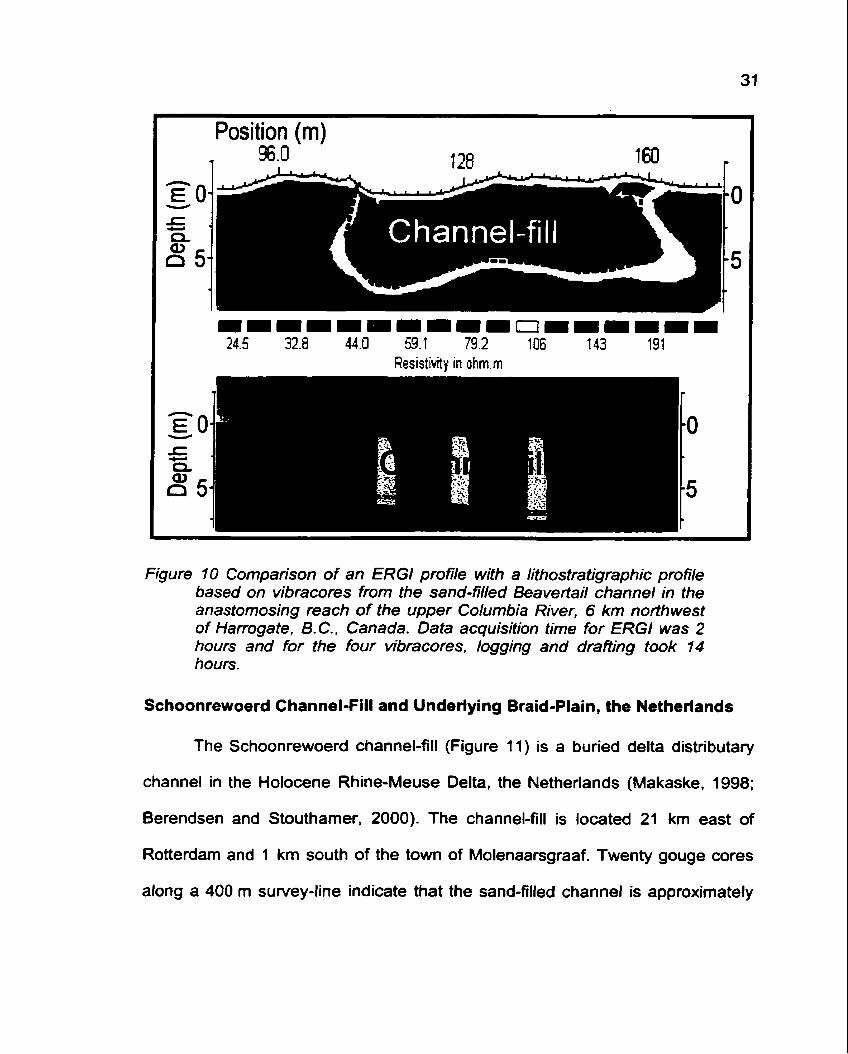
Figure 10 Comparison of an ERG1 profile with a lithostratigraphic profile based on vibracores from the sand-filled Beavertail channel in the anastomosing reach of the upper Columbia River, 6 km northwest of Harrogate, B.C., Canada. Data acquisition time for ERG1 was 2 hours and for the four vibracores, logging and drafting took 14 hours. ............................................................. 31
Figure 11 Comparison of an ERG1 profile with a lithostratigraphic profile based on core data from the Schoonrewoerd channel-fill and underlying Pleistocene braid plain, Rhine-Meuse Delta. The lithostratigraphic profile is adapted from Makaske (1 998) ........................................................................................... 33
Figure 12 Comparison of two perpendicularly intersecting ERG1 profiles on the Beavertail crevasse-splay, upper Columbia River. B.C.. The grey rectangle shows the point of intersection between the two profiles. A comparison between the ERG1 profiles and a lithostratigraphic log from a vibracore at the point of intersection is shown in Figure 14. The discrepancy between these
.................................................. two profiles is explained in the discussion. 38
Figure 13 Comparison of two perpendicularly intersecting ERG1 profiles on the Henon Meadow crevasse-splay, upper Columbia River, B.C.. The grey rectangle shows the point of intersection between the two profiles. A comparison between the ERG1 profiles and a lithostratigraphic log from a vibracore at the point of intersection is shown in Figure 15. ........................ 39
Figure 14 Comparison of the point of intersection between ERG1 profiles BTS201, BTS401, and a simple lithostratigraphic log from the same location. The vibracore at this site only penetrated 4.5 m. The ERG1 profiles have been arbitrarily cut of at around 12 m. See Figure 12 for the full ERG1 profiles. ................................................................................................... 4 1
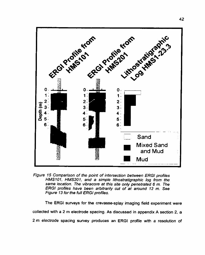
Figure 15 Comparison of the point of intersection between ERG1 profiles HMS101, HMS201, and a simple lithostratigraphic log from the same location. The vibracore at this site only penetrated 6 m. The ERG1 profiles have been arbitrarily cut of at around 12 m. See Figure 13 for the full ERG1 profiles. ....................................................................................................... 42
Figure 16 Photograph of a researcher in chest waders deploying ERG1 equipment from a small boat for the portion of survey line BTC301 that crosses water. Custom-made 2 m long electrode stakes held the sensitive 'smart' electrodes above the surface of the water. ............................... .... 47
viii
Figure 17 ERG1 profile BTC301 compared to a simplified lithostratigraphic profile. The Beavertail sand channel-fill, which is 6.5 to 7 m thick and extends from meter 88 to 135, shows up quite well in this image. Two unnamed channel- fills discovered by Makaske (1998) also are imaged. Many other possible sand bodies appear that are unknown and unverified. The portion of the suwey covered by water extends from meter 147 to 462. Heavy brush was encountered at three locations; meter 64 to 87, 125 to 139, and 482 to 51 7 (see Figure 1 8). .......................................................................................... 4 9
Figure 18 Topographic profile of ERG1 survey BTC301. The water surface in the wetland is higher than the surface of the abandoned Beavertail Channel.
.............................. Elevation in this figure is relative to an arbitrary datum. 59
Figure 19 Comparison of two ERG1 profiles collected with different electrode arrays on the Beavertail channel-fill. The first profile was collected with a 1 m spacing Wenner array and was immediately followed by a 1 m spacing dipole-dipole array survey. A simplified lithostratigraphic profile based on Vibracores and other ERG1 Profiles is included to reference what should be in the 1 m ERG1 profiles. ............................................................................ 62
Figure 20 Comparison of two ERG1 profiles collected with different electrode arrays on the Schoonrewoerd channel-fill and braidplain. The first profile was collected with 10 m spacing dipole-dipole array and was immediately followed by a 10 m spacing Wenner array survey. A simplified lithostratigraphic profile based on hand cores (Makaske, 1998) is included to reference what should be in the 10 m ERG1 profiles. .................................. 63
Figure 21 A conceptual model showing the influence of time related signal noise on the outcome of a comparison between electrode arrays. Here the Wenner array is shown to have less intrinsic noise than the dipole-dipole array, but the comparison is heavily weighted by which array is collected first ............ 65
Figure 22 Timing and duration for the components of the Cumulative Electrode Charge-Up Field Experiment. The electrical contact resistance tests are R1 through R9. The Wenner array surveys are W1 through W4. The Wenner- Schlumberger array surveys are S1 through S4 .......................................... 68
Figure 23 Graph showing the percent bias from the standard for the repeated electrical contact resistance tests (R1 through R9). As R l was the standard for the comparisons, there was 0.00 % bias for R1. .................................... 70
Figure 24 Graph showing the percent bias from the standard for the repeated Wenner (Wl through W4) and Wenner-Schlumberger (S1 through S4) array surveys. As W1 was the standard for the Wenner comparisons, there was 0.00 % bias for W1. The same is true of S1 for the Wenner-Schlumberger corn parisons. . .. . . . . . . . . . . . . . . . . . . . . . . . . . . . ,. . . . . . . . . . . . . . . . . . . . . . . . . . . . . . . . . . . . . . . . . . . . . . . . . . . . . . . . . . 7 1
Figure 25 Graph showing the % RMS model fit for the third iteration of the data inversion for the repeated Wenner (W1 - W4) and Wenner-Schlumberger (S1 - S4) array surveys. ...... ...................................... .................... .... .... ...... 73
Figure 26 Distribution plot of the bias between individual repeated measurements (Wli - W2;) vs. the horizontal location of the measurement along the survey line (X(W1 i)) ........... . .... ...............................---......-........... ............ . . ..-....... 74
Figure 27 Distribution plot of the bias between individual repeated measurements (W 1 i - W2;) vs. the electrode spacing (awl i)) of the measurement. .......... 75
Figure 28 Oblique aerial photograph showing the relative location of the ERG1 study sites on the upper Columbia River in British Columbia. The reach of river shown in the photo is approximately 2.5 km long. .......................... ... 105
Figure 29 Diagram showing the relative location of the ERG1 surveys conducted across the Beavertail channel-fill and area ............................................. 106
Figure 30 A diagrammatic representation of the relative size and location of ERG1 survey series BTC1 and BTC3. Survey BTC301 (series BTC3) was collected for the combination land and water ERG1 survey field experiment (see section 7.1 ). ................ ... ............ ......................... ...... ............... ......... .. ...... 107
Figure 31 ERG1 Survey BTC102. ................................................................ 108
Figure 32 ERG1 Survey BTC103. .................................................................... 108
Figure 33 ERG1 Survey BTC301. ..... . .. . . . . ......... ... . .. . .. . ,. ...... . . . . .. . . . . . . .. . 1 09
Figure 34 ERG1 Survey BML101. .................................................................... 109
Figure 35 Diagram showing the relative location of ERG1 surveys BTS2 and BTS4 on the Beavertail Crevasse-splay. ........ .......... . .. ... ....... .... ...... . . . . 1 10
Figure 36 ERG1 survey BTS2 ... . . . . . .. . . . . . . ... ..... . . . . . . . .. ... ... . . . . . ............... . . . . . . . . . . 1 1 1
Figure 37 ERG1 survey BTS4 ........................................................................... 1 11
Figure 38 Diagram showing the relative location of the 2 ERG1 surveys conducted on the Herron Meadow Crevasse-Splay. ................................. 112
X
....................................................................... Figure 39 ERG1 survey HMS1 11 3
....................................... .............................. Figure 40 ERG1 survey HMSP .. 113
Figure 41 A diagrammatic representation of the relative size and location of the ERG1 surveys on the Schoonrewoerd channel411 ..................................... 115
................... ......................................... Figure 42 ERG1 survey NL9309101 .. 116
Figure 43 ERG l survey NL9309103 ................... ........ ................................... 116
................................................................ Figure 44 ERG l survey NL9309201 117
......................................................................... Figure 45 ERG1 survey CS101 118
Figure 46 ERG1 survey CS102 ......................................................................... 118
Figure 47 ERG1 survey CS103 ....................................................................... 119
Figure 48 ERG1 survey CS104 ..................................... .... .............................. 119
Figure 49 ERG1 survey CS 1 05 ......................................................................... 120
Figure 50 ERG1 survey CS106 ........................................................................ 120
Figure 51 ERG1 survey CS107 ........................................................................ 121
Figure 52 ERG1 survey CS108 ..................................................................... 121

CHAPTER 1. INTRODUCTION
This research tested a new geophysical tool, electrical resistivity ground
imaging (ERGI). to map lithology and geometry of buried deposits of fluvial
sediments. The research included imaging field experiments to determine if ERG1
can detect and delimit fluvial sediments and methodology fieid experiments to
determine procedures for obtaining ERG1 profiles under typical fluvial research
field conditions.
Investigations of fluvial deposits, such as buried mud-encased sand
channel-fills and crevasse-splay sheet-sands, are restricted because of our
limited ability to obtain information about the shallow subsurface. Until recently,
drill cores were the only method available.
Lithostratigraphic logs from boreholes are extremely detailed and have
excellent vertical resolution, but only provide data from one dimension. A series
of boreholes can provide a weak representation of two or three dimensions, but
interpretation is often flawed because the borehole program may not effectively
locate all features, define the lateral extent of features, or discover gradual
changes that occur between boreholes. Borehole programs must balance the
spatial density of the coring program against the time, effort, and cost of each
borehole. If ancillary information about a site was available, coring could be much
more representative and efficient.

Recently, shallow geophysics has offered new methods to obtain
information about the subsurface. Data obtained from shallow seismic and
ground penetrating radar (GPR) have been used to produce two-dimensional
profiles of the subsurface and as a guide for subsequent coring programs. In
many situations, shallow seismic equipment is considered too bulky, heavy, and
expensive for fluvial field work, particularly when travel to and from study sites is
by small water craft or when the equipment must be back-packed over one
kilometer into the survey site. GPR has been used successfully to investigate
fluvial deposits, but requires clean (free of silt and clay) sand and gravel. Clay
and silt attenuate the signal by absorbing the electromagnetic (EM) energy,
which makes GPR mostly ineffective in many fluvial settings such as
anastornosing river deposits (Moorrnan, 1990) and some sand-bed meandering
riven (e.g. the Red Deer and Milk rivers of southern Alberta, D. Smith, pers.
comm., 2001).
ERG1 is a recent addition to shallow geophysics that may be able to
produce effective 20 profiles of buried fluvial deposits in almost all fluvial
settings. ERG1 uses measurements of the electrical resistivity of the subsurface
to produce a two dimensional model of the subsurface called an ERG1 profile.
ERG1 works effectively in clean sand and gravel and in fine sediments such as
silt and clay. This is the first research to use ERG1 to investigate buried mud-
encased sand channel-fills and crevasse-splay sheet-sands.
CHAPTER 2. PREVIOUS RESEARCH
2.1 .I. Electrical Resistivity Ground Imaging
ERG1 is a recent evolution of an old technique. DC-Resistivity, the
precursor to ERGI, uses four electrodes to make a single electrical resistivity
measurement. Subsequent measurements require moving the electrodes to a
new location for each measurement. A set of resistivity measurements is
combined into a plot of either the vertical or the horizontal distribution of
resistivity in the subsurface, and then cuwe matching is used to interpret the data
(Broughton Edge and Laby, 1 93 1 ; Kunetz, 1966). Although both data collection
and interpretation are slow and difficult, the method is still in use (e-g.
El-Hussain, et al, 2000; Maillol et al, 2000).
ERG1 has evolved due to significant improvements to data collection and
interpretation. New computer-controlled multi-electrode systems automatically
collect large data sets without the need to move electrodes (Griffiths et all 1990).
New software packages use 2D finite difference or finite element inversion
routines to produce 2D models of the subsurface (ERGI profiles) (Edwards,
1977; Dey and Morrison, 1979; Barker, 1992; Beard et al, 1996; Loke and
Barker, 1996). Lastly, modem high-speed Pentiurn computers allow for rapid
data processing and manipulation (e.g. topographic corrections, Tong and Yang,
2000). Data collection and processing is now quick, simple, and inexpensive,
while interpretation is straightfoward and reliable (Loke, 2000a and 2000b).

Although ERG1 is increasingly popular for geohydrology, geotechnical
engineering, and environmental consulting (e-g. Dahlin, 1996; Dahlin and Owen,
1998; Maillol et al., 1999; Daily and Ramirez, 2000: Abdul Nassir et all 2000; El-
Behiry and Hanafy, 2000; Gilsom et al., 2000: Maillol et al., 2000; Wolfe et al.,
2000), it is virtually unknown among fluvial geornorphologists and
sedirnentologists. Previously, no published research has used ERG1 to
investigate fluvial sediments such as channel-fills and crevasse-splays.
2.1.2. Anastornosing River Deposits
This research project does not investigate anastomosing river deposits per
se, instead it uses anastomosing river deposits (buried mud-encased sand
channel-fills and crevasse-splays) as a means to investigate and evaluate ERGI.
Nevertheless, a brief discussion of anastomosing rivers is provided.
Since the early 1970s. 'anastomosing rivers' have been accepted by many
researchers as a fourth member of the formerly tripartite river classification of
'straight', 'meandering', or 'braided' riven (Rust, 1978). Under the tripartite river
classification, all multiple channel rivers fell into the braided category. Although
'braiding' implies shallow rapidly evolving channels, some of the rivers grouped
into the braided category had deep stable channels. A new category,
anastomosing, soon became a 'catch-all' for all non-braided multiple-channel
systems. Researchers continue to investigate anastomosing rivers in diverse
continental, climatological, and sedimentological settings to learn more about
their characteristic processes and deposits. An extensive, but not

comprehensive, sample of anastomosing research includes: Leopold et al, 1964;
Smith, 1972; Rust, 1978; Smith and Putnam, 1980; Smith and Smith, 1980;
Quinn, 1982; Locking, 1983; Smith, 1983a and 1986; Moorrnan, 1 990; van Dijk et
al, 1991 ; Harwood and Brown, 1993; Knighton and Nanson, 1993; Tomqvist,
1993; Miall, 1996; Schumm et al, 1996; Weeds, 1996; Berendsen, 1998;
Heritage and Broadhurst, 1998; Makaske, 1998; Abbado and Filgueira-Rivera.
2000; Berendsen and Stouthamer, 2000; Gilvear et al, 2000.
This research loosely follows Smith's (1 986) definition of anastornosing.
For this research, an anastomosing river reach has low-energy, multiple,
interconnected, laterally stable, deep sand-bed channels confined by prominent
silty levees. The levees surround extensive wetlands, marshes, and ephemeral
and permanent lakes. The multiple channels and wetlands usually cover the
entire width of a slowly aggrading floodplain. Typical deposits include buried
mud-encased sand channel-fills and crevasse-splay sheet-sands. Silt and clay
account for 80-90% of the valley-fill in the upper Columbia valley (D. Smith, pers.
comm., 2001).

CHAPTER 3. STUDY SITES
The two study areas for this research project were the anastornosing
reach of the upper Columbia River. British Columbia and the Rhine-Meuse Delta,
the Netherlands (Figure 1). The original selection criterion for study sites was
sites that contained previously studied buried mud-encased sand channel-fills
and crevasse splays. As the project progressed, it became necessary to alter the
criterion and several of the study sites for the project were selected based on
their proximity to sites already in use by the project.
Figure 1 A global view of the ERG1 study sites on the upper Columbia River, British Columbia and on the Rhine-Meuse Delta, the Netherlands.
Study sites on previously studied channel-fills were selected from both
study areas. Although previous research has examined buried crevasse-splays
on the upper Columbia River (e.g. Quinn, 1982), these sites were found to be
difficult to examine with ERG1 (see Chapter 6 section 2 for more details about the
difficulties). Crevasse-splay study sites with no prior subsurface information were
selected within the anastomosing reach of the upper Columbia River that were in
the vicinity of the channel-fill study site previously selected.
3.1. Upper Columbia River, British Columbia
3.1 .l. Regional Setting and Character
The upper Columbia River Rows northwestward through a 100 km
anastomosing reach from Radium Hotsprings, to the confluence with the Kicking
Horse River in the town of Golden, British Columbia. In this reach, the river valley
occupies a portion of the Rocky Mountain Trench (Geological Survey of Canada
1972, 1979a. 1979b. 1980). The Beaverfoot and Brisco Ranges of the Rocky
Mountains (summits up to 2700 m above sea level: asl) border the valley to the
northeast and the Purcell Mountains (summits up to 3000 rn asl) border the
southwest. The valley floor is ca. 790 m (asl), less than 3 km wide, and has an
average gradient of only 12.5 cmlkm (Abbado and Filgueira-Rivera, 2000).
Clague (1975) provides an excellent Quaternary history of the region.
The planforrn of the Columbia River is very complex. Any valley cross-
section typically contains: up to five active channels; numerous buried channels;
a multitude of small lakes, marshes, and mud flats; and a number of active and
abandoned crevasse-splays. Lateral facies changes from sand to mud or vice

versa are abrupt and numerous. Deposits vary from coarse sand in the channels
often with a thin fine-grained (granules and pebbles) gravel lag at the base, silty
fine sand in the crevasse-splays, sandy silt in the levees, silty clay in the
marshes, organic-rich clays in the lakes, to occasional pockets of peat.
Floods inundate the entire anastomosing reach (topping the levees) for
about 45 days per summer (Locking, 1983). The Columbia River has no
engineered water control structures upstream of the anastomosing reach. The
reach is within the Columbia Valley Wetlands Wildlife Management Area and the
Columbia National Wildlife Area, which protects it from development and
precludes shallow seismic surveys.
When we arrived at the upper Columbia River (April 1, 2000), the ground
water level was approximately 80 cm below the ground surface in the abandoned
Beavertail channel. Research at the study site was terminated (May, 24, 2001)
when the river rose high enough to pass-over low points in the levees and flood
all of the practical ERG1 survey sites.
3.1 -2. Survey Locations
Three ERG1 study sites from within the upper Columbia River study area
are included in this thesis (Figure 2): the Beavertail channel-fill, the Beavertail
crevasse-splay, and the Herron Meadow crevasse-splay. The Beavertail channel
and crevasse-splay are located within several hundred meters of the Beavertail
Lodge (532210 5651970 UTM), a trapper's cabin on the main channel of the

Columbia River approximately 7.5 km northwest of the town of Harrogate. The
Herron Meadow crevasse-splay (532414 5651604 UTM) is located on an inter-
channel island between the Baldy Channel and an unnamed channel flowing
along the west valley wall approximately 5.5 km northwest of the town of
Hanogate. The coordinates for all of the ERG1 survey lines and lithostratigraphic
logs from the upper Columbia River presented in this thesis are included in
Appendix D.
Figure 2 Location of the ERG1 study area on the upper Columbia River, British Columbia. The exact locations of all the ERG1 sunleys and lithostratigraphic logs on the upper Columbia River are provided in Appendix 0.
3.2. The Rhine-Meuse Delta, the Netherlands
3.2.1. Regional Setting and Character
The buried mud-encased sand channel-fills and crevasse-splay sheet-
sands in the Rhine-Meuse Delta formed as delta distributary features with
anastomosing character that is attributed to slow continuous sea level rise
throughout the late Weichselian (Wisconsinan) and Holocene (i.e. over the last
18,000 years, Berendsen, 1998). The delta is 130 km long, extending westward
from the German border, where it is 20 km wide, to the North Sea, where it is 60
km wide (H.J.A. Berendsen, pers. wmm., 2000). The delta is slowly filling a
valley bounded by glacial ice-pushed ridges to the north and outcropping
Pleistocene sediments to the south (van Dijk et al., 1991). Under the Holocene
delta is a continuous Pleistocene sand and gravel braid-plain approximately 6 m
below the surface in the east and 22 m below the surface in the west.
The planform of the Rhine-Meuse Delta is very complex, but well known.
Berendsen and Stouthamer (2000) have produced spatially and chronologically
detailed maps of the Paleogeography of the Rhine-Meuse Delta. Through time,
the number of coexistent channels has varied from four to ten (Tomqvist, 1993).
Vast interchannel 'islands' separated the channels, which typically contained
lakes, marshes, mud flats, and peat bogs. Crevasse-splays were infrequent, but
when they did occur, they often formed the basis for a channel avulsion. Because
of the extremely low gradient, many of the distal channels show tidal influence.

Lateral facies changes throughout the delta are frequent and sharp.
Deposits vary from coarse sand in the channels with a thin gravel lag at the base,
through silty fine sand in the crevasse-splays, clayey siit in the levees, silty clay
in the mud flats, to vast areas of peat.
The present Rhioe-Meuse Delta is, in essence, one large engineered
water control structure. Humankind has been directly involved with the hydrologic
behavior of the system since AD 1100 (Berendsen and Stouthamer, 2000).
Nearly all of the delta is developed and has been in use for settlement and
agriculture for many centuries.
All ERG1 surveys in the Rhine-Meuse Delta occurred on low relief (e 40
cm) grass-covered fields used as pastures for dairy cattle. Fields are
approximately 300 m long by 50 m wide, below sea level, and surrounded by 2 to
5 m wide drainage ditches containing 1 to 2 m of water. Pump systems on the
ditches maintain the ground water level approximately 80 cm below the surface.
3.2.2. Survey Locations
Two ERG1 study sites from within the RhineMeuse Delta study area are
included in this thesis (Figure 3): the Schoonrewoerd paleochannel and a
collection of unnamed paleochannels next to the Lek River. The Schoonrewoerd
paleochannel study site (116950 431200 NLRD) is located in a farm field
approximately 1 km south of the town of Molenaarsgraaf and approximately 21
krn east of Rotterdam. The study site on the unnamed paleochannels
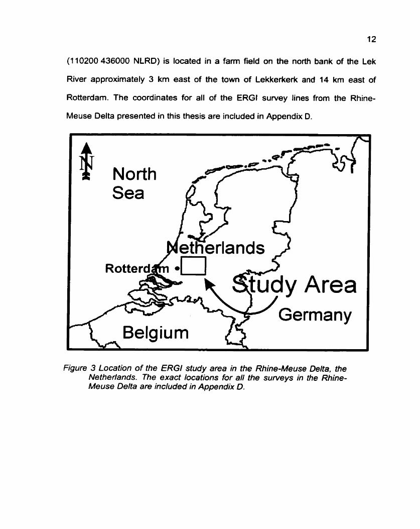
(1 10200 436000 NLRD) is located in a farm field on the north bank of the Lek
River approximately 3 krn east of the town of Lekkerkerk and 14 km east of
Rotterdam. The coordinates for all of the ERG1 survey lines from the Rhine-
Meuse Delta presented in this thesis are included in Appendix D.
Figure 3 Location of the ERG1 study area in the Rhine-Meuse Delta, the Netherlands. The exact locations for all the surveys in the Rhine- Meuse Delta are included in Appendix D.
CHAPTER 4. ERG1 THEORY
Although ERG1 theory and methodology are amply explained elsewhere
(Telford et all 1990; Ward, 1990; Burger, 1992; Reynolds, 1997; Loke, 1999 and
2000), this section provides a summary of the concepts underlying ERG1 data
collection and processing. Practical information about where, when, and how to
conduct ERG1 surveys has been included in appendixes A. B, and C. This
includes 'rules of thumb' regarding the depth and resolution of ERG1 surveys.
4.7. Electrical Resistivity
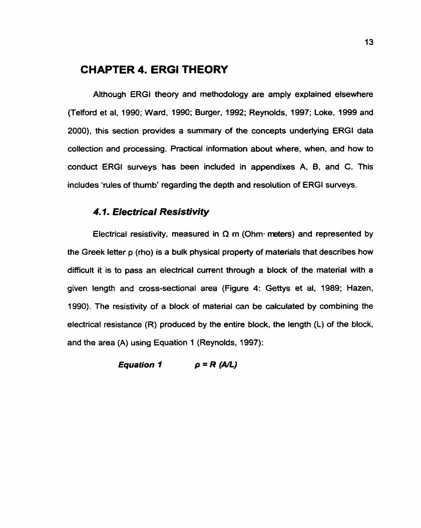
Electrical resistivity, measured in R m (Ohm- meters) and represented by
the Greek letter p (rho) is a bulk physical property of materials that describes how
difficult it is to pass an electrical current through a block of the material with a
given length and cross-sectional area (Figure 4: Gettys et al, 1989; Hazen,
1990). The resistivity of a block of material can be calculated by combining the
electrical resistance (R) produced by the entire block, the length (L) of the block.
and the area (A) using Equation 1 (Reynolds, 1997):
Equation 1 p=R(A/L)
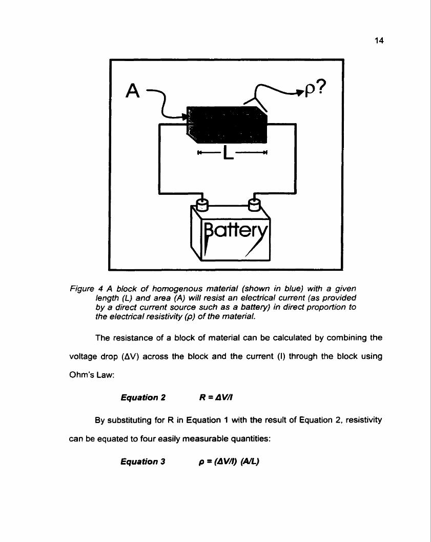
Figure 4 A block of homogenous material (shown in blue) with a given length (L) and area (A) will resist an electrical current (as provided by a direct current source such as a battev) in direct proportion to the electrical resistivity (p) of the matenal.
The resistance of a block of material can be calculated by combining the
voltage drop (AV) across the block and the current (I) through the block using
Ohm's Law:
Equation 2 R = AV/I
By substituting for R in Equation 1 with the result of Equation 2. resistivity
can be equated to four easily measurable quantities:
Equation 3 p = (AVfl) (AR)

Although the resistivity of a block of material is easy to determine, the
resistivity is not enough information to identify the material for two main reasons.
Firstly, materials do not have a unique resistivity 'signature', and many materials
can have the same resistivity (Reynolds, 1997; Loke, 1999). Secondly, the
resistivity of a heterogeneous block of materials is dependant on the resistivity,
proportion, and arrangement of the component materials that make up the block.
In extreme cases, the orientation of the current to the block of material varies the
resistivity measurement obtained from the block. This property, anisotropy, is
common in layered or interbedded sediments (Christensen, 2000).
Resistivity measurements collected as part of an ERG1 survey always
involve heterogeneous conditions, because each measurement is a combination
of the material itself and whatever is within the pores within that material.
Electrolytic conduction (electrical current carried by ions in solution) through pore
water within the pore space in common sedimentary materials dominates their
resistivity measurement. If the groundwater has' consistent ionic content,
resistivity measurements are primarily an indicator of formation porosity,
permeability, and saturation (Archie, 1942). Recognizing the importance of pore
fluids can not be emphasized enough.
4.2. Measuring Electrical Resisfivitjt
The Subsurface.. . .
Figure 5 Electrical resistivity measurements in the field use four electrodes inserted into the ground. Two of the electrodes, A and B, inject current into the ground. The other two electrodes, M and N, are used to measure voltage drop across the surface of the ground.
Electrical resistivity measurements in the field use four point electrodes at
the ground surface (Figure 5). Two of the electrodes. traditionally called A and 6.
introduce a current into the ground, while the other two electrodes, traditionally
called M and N, measure voltage drop. Electrodes A and B are frequently called
the current electrodes, while electrodes M and N are known as the potential
electrodes. Field measurements of current and voltage drop are combined into a
resistivity measurement using a modified version of Equation 3:
Equation 4 p = (AVA) K
K in Equation 4 is a geometric factor that replaces the simple spatial
component of area divided by length in Equation 3. K incorporates the distance
from each current electrode to each measurement electrode and a 'half-space'
term. The half-space terrn is included to accurately model the flow of electricity
downward and outward from each of the four point sources of electrical contact
with the ground.
Equation 5 K = 217 (AM' - ME' - AN' + NE')"
Equation 4 and Equation 5 only hold true when the earth behaves as a
homogeneous half-space. Since the earth is rarely a true half-space (topographic
undulations) and almost never homogeneous, field measurements are
considered apparent resistivity data (p,).
Although Equation 5 works with any arrangement of electrodes,
symmetrical linear arrays are typically used. The arrangement of the four
electrodes used to make an individual resistivity measurement, called an array,
affects the depth of investigation, sensitivity, resolution, and response to noise of
an apparent resistivity measurement. Reynolds (1997) provides an excellent
description of the strengths and weaknesses of the three most commonly used
arrays for ERG1 (Wenner, Wenner-Schlumberger, and dipole-dipole). Appendix B
provides more information about electrode arrays.
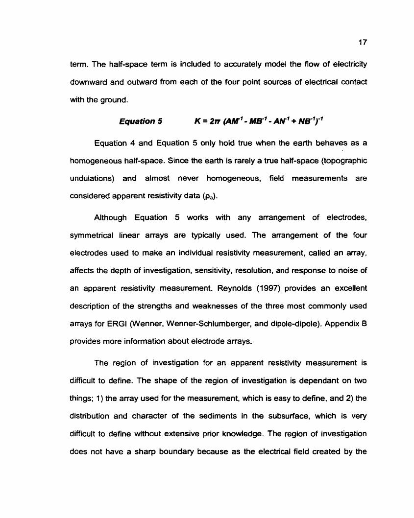
The region of investigation for an apparent resistivity measurement is
difficult to define. The shape of the region of investigation is dependant on two
things; 1) the array used for the measurement, which is easy to define, and 2) the
distribution and character of the sediments in the subsurface, which is very
difficult to define without extensive prior knowledge. The region of investigation
does not have a sharp boundary because as the electrical field created by the
current circuit extends outward and downward from the array it decreases in
strength, but never reaches zero.
Before moving the array
After moving the array
Figure 6 Changing the location of an electrode array, without changing the distance between the electrodes, changes the location of the region of investigation for the resistivity measurement. The depth of the region of investigation does not change. The region of investigation is represented here as an over-simplified sharp-edged round two- dimensional area. In reality, the region of investigation is diffuse, amorphous, and three dimensional.
Although the region of investigation for an apparent resistivity
measurement is difficult to define, there are some simple rules for altering its
location and depth. The location of the region of investigation is simple to move
because its center coincides with the center of the array used to make the
measurement. Thus moving the array without changing the distance between the
electrodes (electrode spacing) moves the region of investigation (Figure 6).
The size of the region of investigation, and therefore the depth, is directly
related to the size of the array. The size of the anay is controlled by the electrode
spacing. Thus increasing the electrode spacing without changing the center point
of the array increases the size, and coincidentally the depth, of the region of
investigation (Figure 7).
Appendix By 'Understanding Electrode Arrays' discusses how multi-
electrode ERG1 systems alter the depth and location of the region of investigation
for apparent resistivity measurements. Appendix A section 2, 'ERG1 Resolution
and Depth of Investigation' discusses guidelines to assess the depth of ERG1
measurements.

L
Electrodes close together
Figure 7 Changing the distance between the electrodes in an electrode array, without changing the location of the center of the array, changes the depth of the region of investigation for the resistivity measurement. The horizontal location of the region of investigation does not change. Note that increasing the distance between the electrodes increases the size of the region of investigation in all directions. This increase in size vastly increases the volume of material contributing to the resistivity measurement.
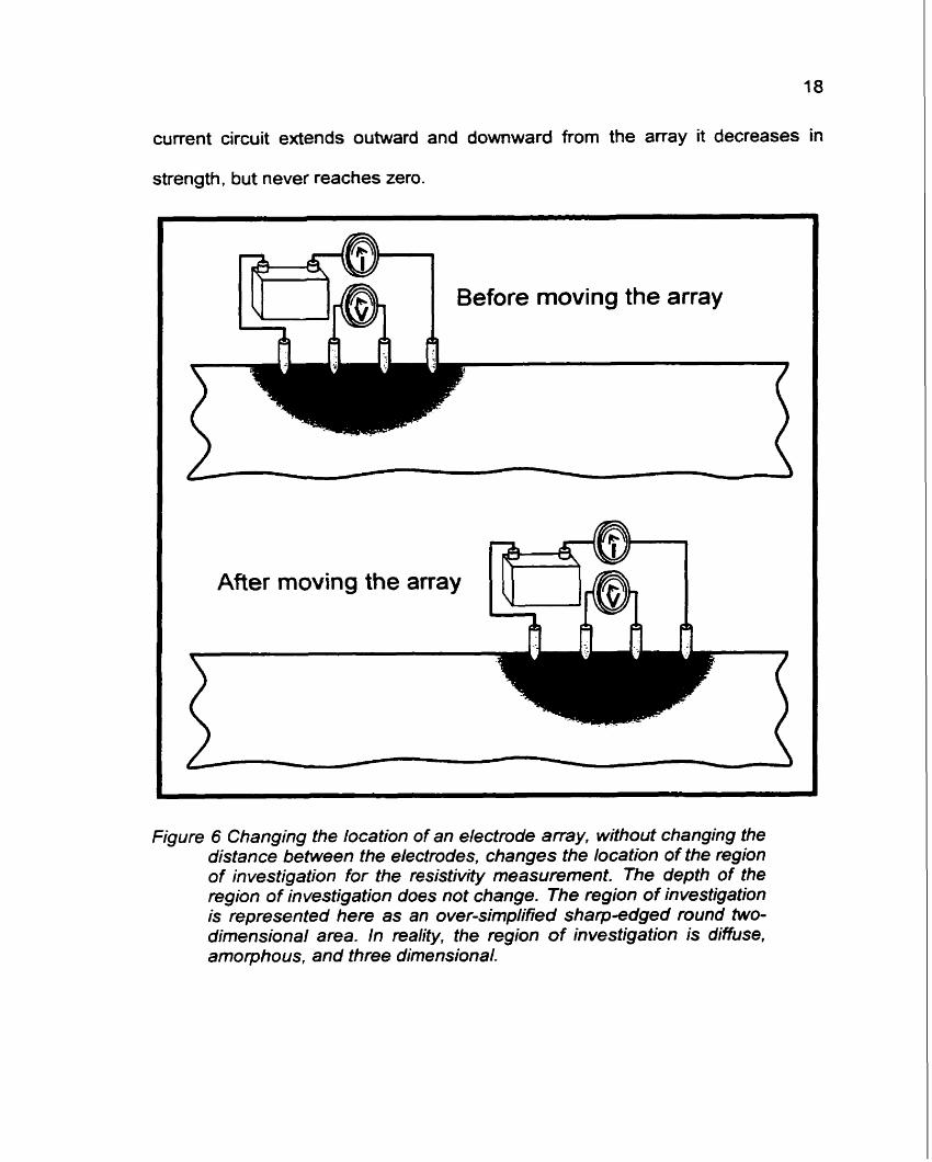
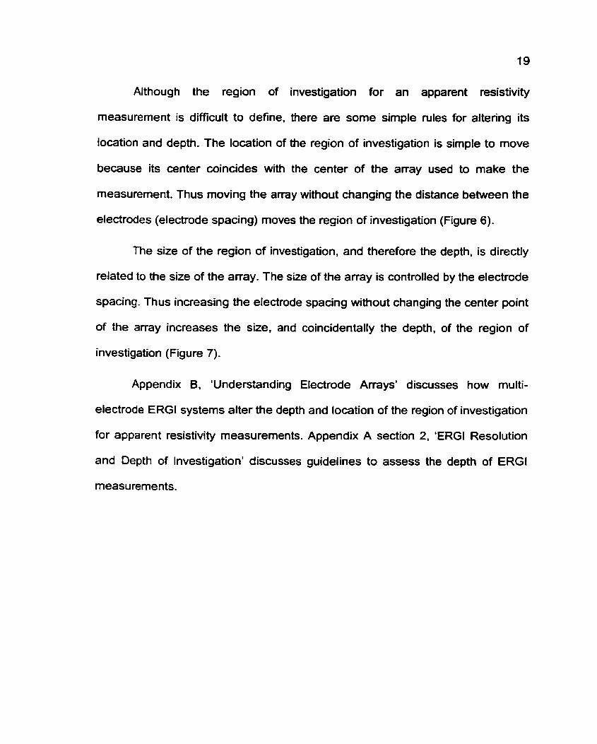
4.3. Ground Imaging with Electrical Resistivity
Figure 8 A diagrammatic representation of a multi-electrode resistivity system used for ERG1 sunleys.
ERG1 involves using a multi-electrode resistivity system (Figure 8) to
collect many apparent resistivity measurements and then processing the data to
produce a two-dimensional profile that shows the variation and distribution of the
true resistivity of the subsurface. A multi-electrode resistivity system uses 56 or
more electrodes and a computer controlled switching unit to collect data from
many different locations and depths by switching which of the electrodes is acting
as the A, the B, the M, and the N electrode for each measurement. Once data is
collected from all depths and locations possible from a single system layout, a
modeling process called 'inversion' is used to convert the apparent resistivity
data into a two-dimensional cross-section image representing an approximation
of the true resistivity distribution in the subsurface.

Inversion is an iterative least-squares process that searches for the
smoothest possible resistivity distribution that would produce the same apparent
resistivity measurements as the field data. Commercially available software
packages, such as RESZDINV (Loke, 2000), use the diffuse amorphous three
dimensional apparent resistivity measurements to generate true resistivity values
assigned to two dimensional model blocks. The value assigned to a two
dimensional model block is only representative of materials at that depth (z) and
horizontal location (x) if there are no resistivity changes to either side of the
survey line (y - the third dimension). For ease of interpretation, ERG1 profiles are
a contoured version of the block model (Figure 9).
Figure 9 Comparison between an inverted resistivity block model and a contoured model. The block model more closely represents the mathematical output of the inversion process, while the contoured model is easier to interpret.

4.4. ERGl Profile Confirmation and Ancillary Data
ERGI, like other geophysical techniques, can not stand alone. ERG1
profiles should be 'ground-truthed' by qualitative comparison with existing
subsurface information (e.g. drill core, electric logs, GPR, shallow seismic,
exposures) whenever possible (Loke. 1 999).
Topographic correction improves the quality of ERG1 profiles, because K
(from Equation 5) requires the ground to be flat and the real world is rarely flat.
This flaUnot flat problem introduces errors that can mask features or generate
artificial features in an ERG1 profile unless corrected (Tong and Yang, 7990;
Loke 1999).
CHAPTER 5. METHODOLOGY
Field experiments performed for this research project were conducted
between April and May 2000 at the study area on the upper Columbia River.
British Columbia, and from late August through September 2000 at the study
area on the Rhine-Meuse Delta, the Netherlands. Each of the field experiments
utilized special methods to address the particular conditions and goals of each
field experiment. The specific methods for each field experiment are discussed
with the field experiment. This section outlines the equipment and general
techniques used for all the field experiments.
To date, no paper outlines ERG1 field procedures. This research project
developed its own procedures through extensive field-testing. These guidelines,
which cover most aspects of ERG1 surveying from site selection to data
processing, are included in Appendix A. Appendix C breaks ERG1 surveying into
12 easy to follow steps.
5.1. ERG1 Data Acquisition
This research project used a 56 electrode AGI StinglSwift R1 Earth
Resistivity Meter to collect the apparent resistivity data. The 56 electrodes are on
four inter-connectable electrode cables with 14 electrodes each. The electrodes
are separated by 12 meters of cable to allow for ERG1 surveys with a 10 meter
electrode spacing across irregular terrain (2 m of excess cable to surmount
obstacles). For ERG1 surveys with smaller spacings. the excess cable is simply
laid out to one side of the survey line.
The AGI system uses 'smart' electrodes. Each 'smart' electrode can be
passive or act as the A, B, M, or N, electrode for a resistivity measurement. The
'smart' electrodes are controlled by a user modifiable command file on the Sting.
See appendix A section 8 for details about creating command files.
The electrodes make electrical contact with the ground by being
connected to a metal spike that has been driven into the ground. Laying the
electrode on a 'shelf, a 10 cm length of angle iron welded across the stake,
provides the electrical connection between the electrode and the stake. The
electrode is held on the 'shelf by an elastic band.
Sometimes the compromise between depth of investigation and resolution
produced an overall electrode line length that was shorter than the horizontal
extent of the intended survey. Conducting 'roll-along' surveys extended the
length of these surveys. A 'roll-along' survey begins by collecting a standard data
set. A number of electrodes, for example 14, are then moved from the beginning
of the survey line to the end of the survey line without moving any of the other
electrodes. Data is again collected in what would be a spatially overiapping data
set; however, a special command file avoids collecting redundant data. This 'hop
scotching' of electrodes from the front of the survey line to the end can be
repeated any number of times and therefore extend a survey line to any length.
Appendix A section 9 provides more details about roll-along surveying for ERGI.
5.2. ERGI Data Inversion
This research project used RES2DINV (Loke, 2000) to invert the apparent
resistivity data. RESZDINV is a large and complex program with many user
modifiable inversion parameters. The software manual provides a detailed
explanation of each parameter and its influence on the inversion process.
While in the field, this research project used a Dell laptop computer
(Pentium 11 266 MHz processor) to invert apparent resistivity data using
RES2DINV's default inversion parameter settings. For all but the largest data
sets, inversions took less than 90 seconds. In the computer lab, a variety of
faster computers was used for further data processing. Appendix A section 7
provides guidelines for ERG1 data processing that were developed during this
project.
5.3. ERGI Profile Confirrnation/Assessrnent
This research project relied on lithostratigraphic log profiles and individual
lithostratigraphic logs for confirmation and qualitative assessment of the ERG1
profiles. Most of the profiles were compared to lithostratigraphic profiles from
previous research at the study sites. Lithostratigraphic profiles from the upper
Columbia River were based on vibracore data, while those from the Rhine-
Meuse Delta were based on cores retrieved with hand tools; the Van der Staay
Suction Corer and the gouge corer. The University of Utrecht has a collection of
200,000 lithostratigraphic logs collected in this way. These logs include 13
different characteristics, including 28 different sediment texture classes. recorded
every ten centimeters (Berendsen, 1994).
No lithostratigraphic data was available for several sites on the upper
Columbia River. Vibracores (Smith 1983b, 1992, and 1998) were obtained to
provide lithostratigraphic logs for confirmation of the ERG1 profiles at these sites.
The vibracores were logged to the nearest 10 cm into five sedimentary
categories: 1) gravel 2) sand 3) mud 4) organic soil 5) intermixed or inter-bedded
(layers less than 10 cm thick) sand and mud.
5.4. Locational Data Acquisition
This research project used a hand-held GPS receiver to obtain
coordinates for the ends of all the ERG1 surveys and for all of the coring
locations. UTM coordinates were used on the upper Columbia River. NLRD
coordinates were used on the Rhine-Meuse Delta. No corrections were applied
to the GPS positions, and a k 6 m positional error is assumed (Federal Geodetic
Control Subcommittee and GPS Interagency Advisory Council, 2000). All the
locations for the surveys presented in this document are included in Appendix D.
5.5. Topographic Data Acquisition
This research project used a David White laser auto-leveler to collect
topographic profiles of the ERG1 survey lines. The topographic data was
collected at 'nick-points' in the terrain, as described in the RES2DINV manual
(Loke, 2000).
CHAPTER 6. IMAGING FIELD EXPERIMENTS
The goal of the imaging field experiments was to determine if ERG1 can
detect and delimit fluvial sediments. This section describes field experiments to
image buried mud-encased sand channel-fills and to image crevasse-splay sheet
sands.
6.1. Channel-Fill Imaging Field Experiment
The goal of this field experiment was to determine if buried mud-encased
sand channel-fills could be imaged with ERGI. Many channel-fills were
investigated on the upper Columbia River. B.C.. and the Rhine-Meuse Delta, the
Netherlands. One representative case from each of these areas is presented:
survey line BMLlO1 from the Beavertail Channel and survey line NL9309201
from the Schoonrewoerd channel-fill and braid-plain.
6.1.1. Methods for this Field Experiment
The data for the ERG1 profile for the Beavertail Channel was collected
using a Wenner array on a 56 electrode survey with a 2 rn electrode spacing.
Three 14 electrode 'roll-along's extended the survey line to 194 m in length. The
command files were designed to measure information from up to 18 m depth.
The Beavertail Channel-fill presented several data collection challenges.
The 14 m stretch of open sand in the remnant Beavertail Channel (meter 103 to
meter 1 17) made achieving sufficiently low electrical contact resistance difficult.
Low contact resistance was maintained by flooding a 30 cm wide by 10 cm deep
trench with saline solution. For more information on electrical contact resistance,
see appendix A section 4.
The heavy brush and deadfall on the levees made travel along the survey
corridor and placement of the electrodes difficult. To alleviate this, a 2.5 m wide
survey corridor was cleared through the brush on the levees. Large deadfall was
removed from the survey corridor when it blocked travel along the survey line
and when it was directly in the way of an electrode stake.
The data for the ERG1 profile for the Schoonrewoerd channel-fill was
collected using a Wenner array on a 56 electrode survey line with a 2 m
electrode spacing. The survey line was 1.10 m long and designed to collect
information from up to 18 m deep. There were no electrical contact resistance
problems, topographic issues, or challenging ground cover types encountered in
the Netherlands.
Beavertail Channel-Fill, British Columbia
The Beavertail channel-fill (Figure 10) is a partially abandoned anabranch
of an anastornosing river depositional system of the upper Columbia River,
British Columbia The channel-fill is located mid-valley 6 km northwest of the
hamlet of Harrogate. The Columbia River only flows through the channel during
flood discharge, usually from June 1 to July 30. Four vibracores indicate the

sand-filled channel varies between 6 and 7 m thick by 45 m wide. The 45 m width
was inferred from topography and vegetation changes at the suspected channel
margins (D. Smith, pers. comm., 2001). The channel-fill is almost encased in
clayey-silt except for 14 m of open sand at the surface (channel 4 in Makaske,
1 998).
The ERG1 profile at this site nearly duplicates the lithology and geometry
of the channel-fill as interpreted from vibracores. In the ERG1 profile, the channel-
fill has a thickness between 6 and 7 m and a width of 46 m. While vibracores
provide excellent vertical resolution (direct measurement of core barrel
penetration), ERG1 provides better lateral resolution (-1 m), which is far superior
to any coring method. This latter point is important for precise delineation of
channel-fill margins in anastomosing and deltaic distributary systems where
lateral accretion is limited. In this case, the ERGI-based channel width is likely
more reliable than the inference based on topography and vegetation. Had the
channel-fill had been more deeply buried, the 45 m width could not have been
inferred from topography and vegetation, but ERG1 would still have provided an
accurate estimate.
Position (m) C
-0
-5 .
m I I = m I m . ~ m = m 24.5 32.8 44.0 59.1 79.2 1 06 1 43 191
Resistivity in 0hrn.m
m
-0
-5 .
Figure 10 Comparison of an ERG1 profile with a lithostratigraphic profile based on vibracores from the sand-filled Beavertail channel in the anastomosing reach of the upper Columbia River, 6 km northwest of Harrogate, B.C., Canada. Data acquisition time for ERG1 was 2 hours and for the four vjbracores, logging and drafting took 14 hours.
Schoonrewoerd Channel-Fill and Underlying Braid-Plain, the Netherlands
The Schoonrewoerd channel-fill (Figure 11) is a buried delta distributacy
channel in the Holocene Rhine-Meuse Delta, the Netherlands (Makaske, 1998;
Berendsen and Stouthamer, 2000). The channel-fill is located 21 km east of
Rotterdam and 1 km south of the town of Molenaarsgraaf. Twenty gouge cores
along a 400 m survey-line indicate that the sand-filled channel is approximately
65 m wide by 8.5 m thick. Its top is 1.5 m below the surface and its base is 2 m
above the Pleistocene braidplain. There are no topographic or vegetation
changes to suggest the locations of the channel margins. The channel-fill is
encased in clay and peat with siltylsandy-clay levee 'wings' (Makaske, 1998).
The lithoarchitecture of this site, as indicated by the lithostratigraphic profile, is
perfect for testing ERG I.
The ERG1 profile at this site approximately duplicates the lithology and
geometry of the channel-fill as interpreted from the cores. The ERG1 profile also
detects the basal Pleistocene braidplain sand and gravel. The profile does not
show the left side of the channel-fill because a water-filled ditch and adjacent
road prevented further data collection. In the ERG1 profile, the channel-fill is 9 m
thick by 68 m wide and the braidplain sand and gravel is 12 m below the surface.
Again, there is remarkable correspondence between the ERG1 profile and the
interpreted lithology and geometry of the Schoonrewoerd channel-fill. It is
important to note that the ERG1 data was collected and processed in less than
10% of the time taken for coring.

6.2. Crevasse-Splay lmaging Field Experiment
Our understanding of buried mud-encased crevasse-splay sheet-sands
and their possible interconnections with channel sands is limited because they
are so hard to study. In anastornosing settings, crevasse-splays buried under
more than a meter of clay and silt have almost no surface expression and are
extremely difficult to locate. If ERG1 can image deeply buried crevasse splays, it
could be used as a prospecting tool to locate and then study these deposits.
However, preliminary investigations to assess the ability of ERG1 to image
crevasse-splays is necessary before carrying out an extensive prospecting
campaign.
Shallow buried crevasse-splays can be located because they have
visually apparent topographic expression and they are typically heavily wooded
due to their drainage advantage over the mudflats. Although near-surface buried
crevasse-splays are simple to locate, they are a poor choice for ERG1
investigations because ERG1 is extremely dimcult in thick wood cover. Before
clearing vast stretches of woody vegetation for a study of shallow buried
crevasse-splays, preliminary investigations to assess the ability of ERG1 to image
surface crevasse-splays was in order.
The goal of this field experiment was to determine if surface crevasse-
splay sheet-sands overlying organic-rich muds could be imaged with ERGI. Two
crevasse-splays in the upper Columbia River, B.C., were investigated with nine
ERG1 surveys and 15 vibracores. Two ERG1 profiles from the Beavertail
crevasse-splay (BTSZO1 and BTS401) and the two ERG1 profiles from the
Herron Meadow crevasse-splay (HMS101 and HMSPOI) are presented.
6.2.1. Methods for this Field Experiment
The ERG1 surveys for this field experiment intersect each other at 90" and
provide a certain amount of collateral interpretation support. A lithostratigraphic
log obtained at the intersection point of the paired surveys is included to assist
with qualitative assessment of the ERG1 profiles.
For the stretches of open sand. sufficiently low electrical contact
resistance was maintained by flooding a 30 cm wide by 10 crn deep trench with
10 Um of saline solution the day before data was collected. Touch ups with 1 to
2 L of saline solution per electrode were often necessary on the day of data
collection. For more information on electrical contact resistance, see appendix A
section 4.
On the Beavertail crevasse-splay, the data for survey line BTSZOl was
collected using a Wenner array on a 54 electrode survey with a 2 rn electrode
spacing. The survey was designed to be 106 m in length and to measure
information from up to 16 m in depth.
BTSPOl extends outward from the levee breach past the toe of the
crevasse-splay and abuts a small lake. BTS401 crosses a wide mudflat before
passing over the crevasse-splay perpendicularly to BTS201. The intersection
between survey line BTS201 and BTS401 is at meter 73 on BTS201 and at
meter 105.5 on BTS401.
The data for survey line BTS401 was collected using a Wenner array on a
56 electrode survey with a 2 m electrode spacing. One 14 electrode 'roll-along'
extended the survey to 138 m in length. The command file for-the survey was
designed to measure information from up to 18 m in depth.
On the Herron Meadow crevasse-splay, the data for survey line HMSlOl
was collected using a Wenner array on a 51 electrode survey with a 2 m
electrode spacing. The survey was designed to be 100 m in length and to
measure information from up to 16 m in depth.
HMSlOl extends outward from the levee breach past the toe of the
crevasse-splay and abuts the levee on the far side of the island. HMS201
straddles the crevasse-splay perpendicularly to BTSPOl and extends into the
mudflats on either side. The intersection between survey line HMSlOl and
HMS201 is at meter 23.3 on HMS101 and at meter 55 on HMS201.
The data for survey line HMSZOl was collected using a Wenner array on a
56 electrode survey with a 2 m electrode spacing. The survey was designed to
be 110 m in length and to measure information from up to 18 m in depth.
The crevasse-splays show up very well in the ERG1 profiles. The
horizontal extent of the crevasse-splays is portrayed very accurately. The vertical
extent of the crevasse-splays is exaggerated, but explainable. Explained and
unexplained high resistivity anomalies also appear in the ERG1 profiles.
The horizontal accuracy of the ERG1 profiles is exceptional. Surficial
geology changes indicate that the Beavertail crevasse-splay is 89 m long by
47 m wide, which is the same as what is shown in the ERG1 profiles (Figure 12).
Similarly, the Herron Meadow crevasse-splay is shown by surficial geology
changes to be 43 rn long by 45 m wide, while the ERG1 profiles indicate that the
splay is 44 m long by 45 m wide (Figure 13). This correspondence between
ERG1 profiles and the surficial geology reinforces the findings of the channel-fill
field experiments that ERG1 has an untapped potential for delineating the
horizontal extent of fluvial deposits.
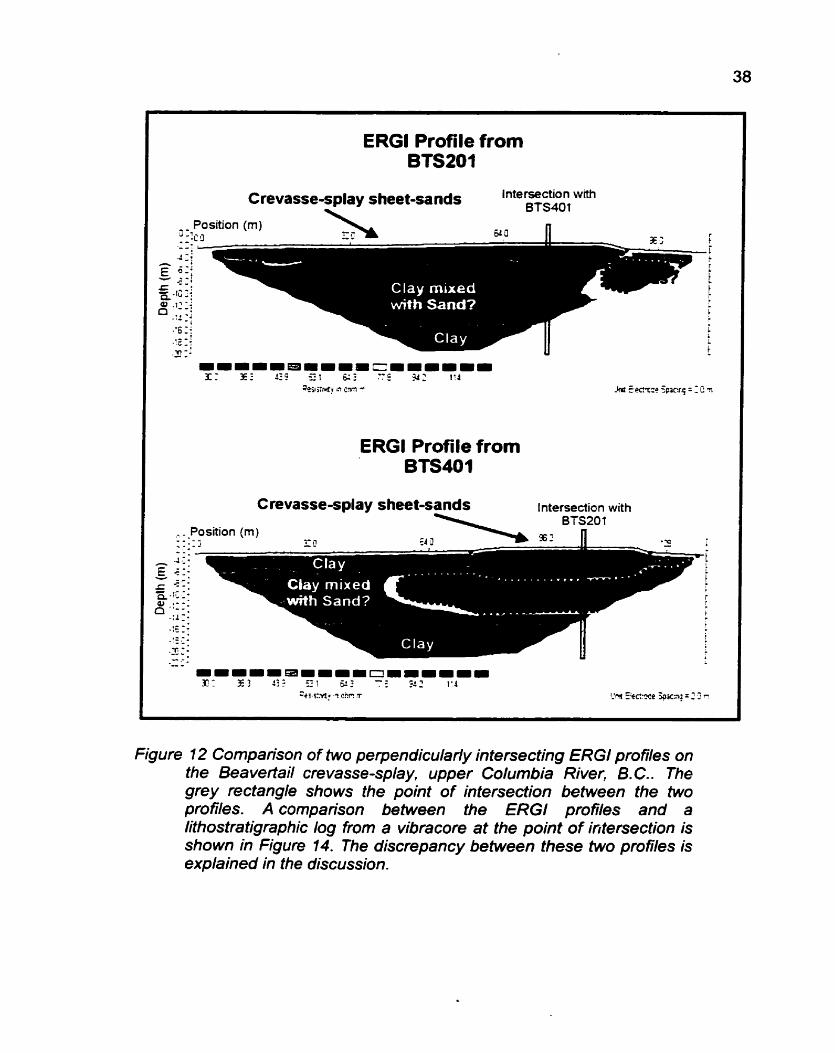
Figure 1 2 Comparison of two perpendicularly intersecting ERGl profiles on the Beavertail crevasse-splay, upper Columbia River, B. C.. The grey rectangle shows the point of intersection between the two profiles. A comparison between the ERGl profiles and a lithostratigraphic log from a vibracore at the point of intersection is shown in Figure 14. The discrepancy between these two profiles is explained in the discussion.
i
h
ERG1 Profile from BTSZO?
Crevasse-splay s heet-sands Interrection with BTS4Ol
r L
i t 1 i i t t
m m m m m 3 - = - m - m X: Ez C4 1 7'5 174
7e~j;wf n irnm -I .Ins Ewz:? 5p1c:q = I C 3
ERG1 Profile from BTS401
Crevasse-splay sheet-sands Intersection with
- -Position (m ) - - - - .- - i - - 4,:: !
E : : Y
r '1: E = - I 5 :: ;
Q, + - - .
; a -;i::
- 3 - ! .YE z - .,:,-. - - .T -. -- - - .- . L - -
= = = m ~ r n u ~ = ~ = m ~ 3 3 23: Et - 3 5:: 1.4
Z c i 5:.xl! .- cCt! s y~ E i e ~ r ~ e = 2 ; 7
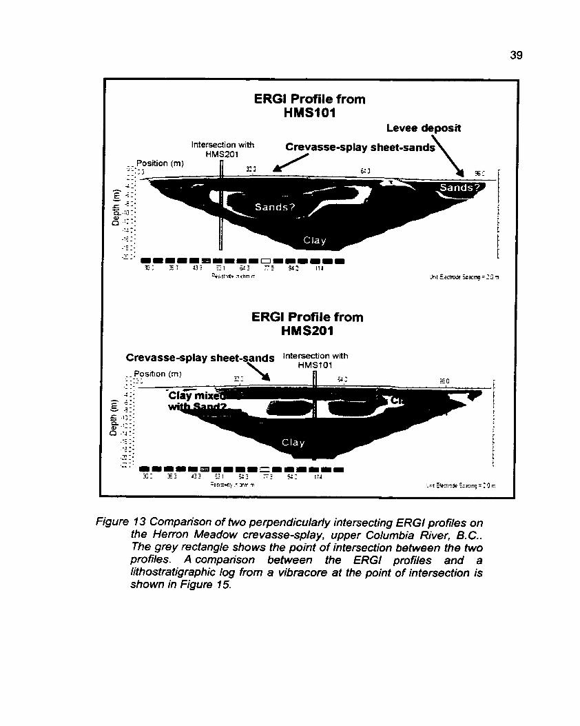
Figure 1 3 Comparison of two perpendicularly intersecting ERGl profiles on the Herron Meadow crevasse-splay, upper Columbia River, B. C.. The grey rectangle shows the point of intersection between the two profiles. A comparison between the ERGl profies and a lithostratigraphic log from a vibracore at the point of intersection is shown in Figure 15.
ERG1 Profile from HMSjO1
Levee deposit Intersection with Crevasse-splay sheet-sands
HMS201 - Position (m)
I m o m m m m m m : r; zt 3: 7 3 Y' I r r
? i i , 3 d v 3 cnn rr 2nd E:eamde jpcmq = 2 S ZI
ERG1 Profile from HMS201
, - Position (m) , .- - - - .J 4 .- -.
L - - - - I - - r r r r m z = - = m m m x - E: r:? 1 3: 7 3: I:;
= e s ~ s t q .r I ~ T .r: I.rn aartmde C:a:~r$ = 9 IT
*
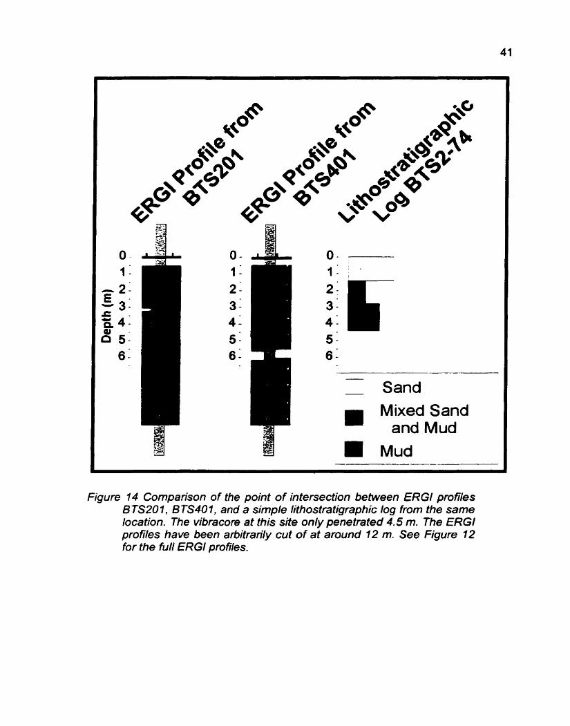
In this case. the crevasse-splay vertical extent (thickness) estimates
based on the ERG1 profiles are exaggerated. Although a lithostratigraphic log
shows the Beavertail crevasse-splay to be 1.4 m thick (Figure 14), the ERG1
profiles show it to be either 2.5 m thick (BTS401) or 3.0 rn thick (BTSZOI).
Similarly. a lithostratigraphic log shows the Herron Meadow crevasse-splay to be
0.7 m thick (Figure 15), while both the ERG1 profiles show it to be 1.5 m thick.
The thickness discrepancy between the lithostratigraphic logs and the
ERG1 profiles is attributable to the extremely high resistivity of the dry sand within
the crevasse-splay and the choice of electrode spacing. The resistivity for the dry
sand within the crevasse-splays was modeled as high as 2237 R m on the
Beavertail crevasse-splay and 1 192 n m on the Herron Meadow crevasse-splay.
This is from 30 to 55 times higher than the clay found below the crevasse-splay
(typically 4 40 f2 m). Such extreme resistivity contrasts produce 'shadowing'
below high resistivity zones within an ERG1 profile, which increases their
apparent thickness. In this case the 'shadowing' may have doubled the apparent
thickness of the crevasse-splay in the ERG1 profiles. However, because
shadowing is a consistent phenomenon, the lithostratigraphic logs could be used
to produce a much more vertically accurate interpretation of the ERG1 profiles.
0 - 0 - 1 - 1 - ' .
2 - 3: 4 - 5 - 5 - 6: 6 1
- Sand -
Mixed Sand and Mud
Mud - -----
Figure 14 Comparison of the point of intersection between ERG1 profiles BTS201, B TS40 1, and a simple lithostratigraphic log from the same location. The vibracore at this site only penetrated 4.5 m. The ERG1 profiles have been arbitrarily cut of at around 12 m. See Figure 12 for the full ERG1 profiles.
4 - 5 -
- - Sand
Mixed Sand and Mud
Mud
Figure 15 Comparison of the point of intersection between ERGl profiles HMS 10 1, HMSPO 1, and a simple lithostratigraphic log from the same location. The vibracore at this site only penetrated 6 m. The ERGl profiles have been arbitrarily cut of at around 12 m. See Figure 13 for the full ERGl profies.
The ERG1 surveys for the crevasse-splay imaging field experiment were
collected with a 2 m electrode spacing. As discussed in appendix A section 2. a
2 m electrode spacing survey produces an ERG1 profile with a resolution of
approximately 2 1 m. Generally, to define an object within an ERG1 profile. it
should be at least 2 or 3 times larger than the resolution. The crevasse-splays
surveyed for this field experiment were only 0.7 to 1.4 times larger than the
resolution of the electrode spacing used. These surveys were conducted before
the full impact of electrode spacing was understood. Repeating these surveys
with a smaller electrode spacing would produce much better vertical thickness
estimates.
The ERG1 profiles for the crevasse-splay imaging field experiment contain
several high resistivity anomalies that are indicative of sand or gravel other than
the crevasse-splays themselves. Some of these anomalies are explained here
while others have been left to future researchers for exploration and explanation.
A simple to explain anomaly is the high resistivity zone extending into
HMSl 01 (Figure 13) from the right. This anomaly is under a slight topographic
rise leading to the heavily vegetated levee adjacent to the Baldy Channel of the
Columbia River. The location of the anomaly suggests that it is a 'levee wing'
deposit (Makaske, 1989).
A more complex explanation is required for the high resistivity anomalies
centered 4.5 m below meter 93 on BTS201 and 8 m below the surface from
meter 54 to the end of BTS 401 (Figure 12), which are most likely caused by the
same sedimentary feature. This explanation relies on the inability of ERG1 to
correctly represent lithology changes that occur to either side of a survey line. A
sedimentary feature, such as a sand or gravel body, located parallel to a survey
line is incorporated into the resulting ERG1 profile as a high resistivity anomaly at
a depth proportional to the distance from the survey line to the feature.
Lithostratigraphic log BTS2-92 confirms that survey line BTS201 crosses a near-
surface buried sand and gravel body which is most likely a small channel-fill at
meter 93. Given that this feature is to one side of BTS401, it was included as the
deeper anomaly in that profile.
Three dimensional dilemmas, such as the one discussed here, can be
solved by comparing intersecting surveys with support from lithostratigraphic
logs. For a more intensive solution to this type of dilemma. ERG1 can be
collected and processed fully in three dimensions.
The high resistivity anomaly centered at approximately 6 m depth below
the Herron Meadow splay in profiles HMSlOl and HMSPOl (Figure 13) is most
likely a buried crevasse-splay, but has not been confined. Future researchers
could use a deeper coring tool than was used for this research project to explore
and explain these anomalies.
CHAPTER 7. METHODOLOGY FIELD EXPERIMENTS
The goal of the methodology field experiments was to determine
procedures for obtaining ERG1 profiles under typical fluvial research field
conditions. This section describes field experiments to combine land and water
within an ERG1 survey, to determine the best electrode array for imaging fluvial
sediments, and to assess long-term cumulative electrode charge-up effects on
repeated ERG1 surveys on the same survey line.
Although informal and anecdotal field experiments to determine
procedures for obtaining ERG1 profiles under typical fluvial research field
conditions are not reported, the resultant improvements to ERG1 procedures from
said experiments have been included in Appendixes A, B, and C.
7.1. Combination Land and Water ERG1 Survey Field
Experiment
The landscape encompassing an anastomosing river reach contains so
many river channels, lakes, and marshes that any lengthy straight line, such as
an ERG1 survey line, crosses both dry land and open water. Although techniques
exist for ERG1 surveys on dry land or under water, there are no techniques for
surveying a combination of land and water. The main challenge facing
combination land and water ERG1 surveys lines is the special equipment and
data processing required for underwater surveys. Underwater electrodes are
rugged and watertight with sealed connections to robust heavily-insulated cables.
Data inversion of the undewater apparent resistivity measurements requires a
correction for the depth and resistivity of the water above each electrode. This
correction remedies the false assumption in equation 5 that above the survey line
is an infinite hemisphere with infinite resistivity, in other words: air.
This field experiment tested the use of modified land surveying techniques
and equipment to obtain an ERG1 profile from a survey line that combined both
dry land and open water. Survey line BTC301, located on the Beavertail channel
and adjacent wetlands, ran ENE from the edge of the main channel of the
Columbia River, across a mudflat (the bottom of an ephemeral lake), an
abandoned channel and its levees, a lake and a marsh (4 .7 m deep), a small
(10 m wide by 50 cm deep) channel and its levees, and eventually abutted the
Hogranch Channel of the Columbia river.
7.1 .I. Methods for this Field Experiment
The combined land and water ERG1 profile data was collected using a
Wenner array on a 56 electrode survey line with a 5 m electrode spacing. Two 28
electrode 'roll-along's extended the survey line to 555 m in length. The command
files were designed to measure to 20 m depth. The survey line preparation and
data collection occurred over a two week period starting April 9, 2000.
For the portion of the survey line crossing land, the experiment used
standard ERG1 surveying techniques. A 2.5 m wide survey conidor was cleared
through the brush on the levees. Large deadfall was removed from the survey

corridor when it blocked travel along the survey line and when it was directly in
the way of an electrode stake.
For the portion of the survey line crossing water, researchers in chest-
waders deployed the stakes and cables from a small boat. Experimental 2 m long
aluminum electrode stakes held the electrodes above the surface of the water
(Figure 16).
Figure 16 Photograph of a researcher in chest waders deploying ERG1 equipment from a small boat for the portion of survey line BTC301 that crosses water. Custom-made 2 m long electrode stakes held the sensitive 'smart' electrodes above the surface of the water.
Standard data processing techniques were used to produce the combined
land and water ERG1 profile. No compensation was made to account for the
portions of the survey crossing open water. The water layer (4 -7 m thick) was
thinner than the resolution of the survey (-2.5 rn) and was not expected to
appear in the profile.
Four vibracores from the Beavertail channel-fill and several sporadically
spaced hand cores from Makaske's (1998) study of the same survey line were
used to qualitatively 'ground truth' the profile.
7.1 -2. ResultslDiscussion
Although the Beavertail channel-fill is fairly well represented in the
combined land and water ERG1 profile (BTC301), the rest of the image is difficult
to interpret (Figure 1 7).
The combined land and water ERG1 profile failed to produce a well
'ground-truthed' clear profile for two main reasons. Firstly, the 'ground-truthing'
information lacked density and depth. Secondly, the field conditions and the
equipment used for the resistivity measurements lead to unreliable noisy data
that the data inversion was unable to correctly process.
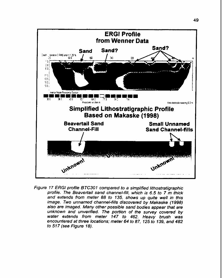
from Wenner Data
I.+& ?lrctrode soacm3 5 3 m
Simplified Lithostratigraphic Profile Based on Makaske (1 998)
Beavertail Sand Small Unnamed
Figure 17 ERG1 profile BTC307 compared to a simpljfied lithostratigraphic profile. The Beavertail sand channel-fill, which is 6.5 to 7 m thick and extends from meter 88 to 135, shows up quite well in this image. Two unnamed channel-fills discovered by Makaske (1 998) also are imaged. Many other possible sand bodies appear that are unknown and unverified. The portion of the sunfey covered by water extends from meter 147 to 462. Heavy brush was encountered at three locations; meter 64 to 87, 125 to 139, and 482 to 51 7 (see Figure 18).
'Ground-Truthing' Problems
The 'ground-truthing' problems faced by the combined land and water
ERG1 profile stem from problems with the coring strategy and techniques. The
coring strategy of the pre-existing core data led to poor lateral data density.
Limitations to the coring technique preempted improving some of the data
density problems. Limitations to the coring technique also prevent core data from
providing good vertical coverage.
Coring strategies based on even spacing, or on specific targets suggested
by surficial morphology (such as topography or vegetation changes), frequently
miss sub-surface features or poorly assess their horizontal extent. ERG1 profiles
have very high lateral resolution and effectively delineate all features under the
survey line. Coring at the density of an ERG1 profile would be prohibitively
expensive and time consuming. A targeted coring program based on an ERG1
profile would be a much better 'ground-truthing' approach than using preexisting
low-lateral-density core data. This is an important concept, which is contrary to
most geomorphic studies, but is commonly employed in the oil industry where
seismic surveys are conducted to determine the most suitable location for drilling.
The coring strategy for a combined land and water survey line is
constrained by limitations to the coring technique used. Vibracoring and hand
coring are the only suitable wring techniques for remote sites such as the
Beavertail channel-fill, but neither technique works in deep open water. This
explains the lack of core data from approximately meter 150 to meter 390 in the

pre-existing core data and why no cores were collected in this region as a part of
this field experiment. However, this also leaves less than one half of the lateral
extent of the survey line 'ground-truthed'.
Vibracoring through deep water is possible from an ice-covered surface.
ERGI, on the other hand, works much better before freeze-up. A two-season field
campaign could provide a combined land and water ERG1 profile with 'ground-
truthing' that has sufficiently high lateral density and coverage- However, 'quick
and dirty' studies are currently not possible.
A second limitation to the coring techniques used to ground-truth the ERG1
profiles is the maximum penetration depth of cores. A common working depth for
both hand cores and vibracores is around 6 meters. Cores up to 18 m deep are
possible, but are time and labor intensive (D. Smith, pers. comm., 2001). ERG1
profiles can easily image down to 90 m. Much of the information presented in an
ERG1 profile is too deep to be ground-truthed with hand cores or vibracores.
The combined land and water ERG1 profile provides information that is up
to 20 m deep, but the pre-existing core data is all less than 8 m deep, and much
of it is less than 4 m deep. Consequently, far less than one half of the vertical
extent of the profile is 'ground-truthed'.
Overall, problems with the coring strategy and technique left the combined
land and water ERG1 profile with poor ground-truthing that covered less than one
sixth of its area. A post-freeze-up targeted vibracoring program that would have
the vastly improved the quality and extent of the ground truthing was not
attempted. The extra effort would have been wasted because the profile was
critically flawed by poor data caused by data collection problems.
Data Collection Problems
The data collection problems faced by the combined land and water ERG1
profile stem from specific field conditions and from the apparent resistivity
measurement equipment. The problematic field conditions encountered on land
included frost and thick beds of matted vegetation; in the water the loosely
compacted organic-rich silts on the lake bottom created problems. The main
equipment problem stemmed from the experimental 2 m long aluminum
electrode stakes.
The combined land and water field experiment was collected very eady in
the summer and thick frost was encountered in the shade of the vegetation on
the levees. Particularly solid patches of frost were discovered under any of the
deadfall removed from the survey corridor. There is very little electrical contact
between frozen ground and an electrode stake. If the contact resistance can be
lowered enough to allow data collection, the resultant ERG1 profile will include
the highly resistive frost layer. Patchy frost shows up in ERG1 profiles as near
surface odd shaped high resistivity blobs that can distort the entire image (Ritz et
al, 1999).
The frost problems on the combined land and water survey were
compounded by the combination of the increasingly warm weather and the
removal of vegetation and deadfall from the survey corridor. Not only was the

frost discontinuous, but also its extent was shrinking day-to-day and hour-by-
hour. The melting of the frozen zones led to variable electrical contact resistance,
unstable currents during the measurement process, and smaller and smaller
resistive zones affecting each subsequent apparent resistivity measurement. See
appendix A section 4 for more about contact resistance and appendix A section 5
for more instrument errors caused by fluctuating currents.
Contact resistance problems were also caused by repeating layers of
overbank mud, leaf matter, woody debris, roots, and stems covering the levees.
The woody debris and roots made inserting the electrode stakes difficult. The
combination of roots, stems, woody debris, and leaf matter provided an excellent
insulator which lead to high apparent resistivity measurements and high electrical
contact resistance. When the top layer of matter was removed in the hopes of
exposing the 'ground surface', more layers of insulating material were
discovered. Occasionally, the 2 m long aluminum electrode stakes were used in
an attempt to penetrate through to the sediments beneath the electrically
insulating ground cover. These efforts met with limited success mostly due to
problems with the 2 m long aluminum electrode stakes, which will be discussed
shortly.
The resistivity of the water layer varied over short time periods due to the
passage of the researchers along the survey line stimng up the organic-rich silt
on the lake bottom. Stimng up the bottom sediments lowers the resistivity of the
water because suspended sediments can cany electrical current through water.

As the sediments settle out, the resistivity of the water drops. Thus, the passage
of a researcher along the survey line to set up equipment, to troubleshoot
equipment, or to retrieve equipment alters the data collected. Presumably, a
limited number of field tests could determine a suitable settling intewal to wait
between stirring up the bottom and collecting data. Underwater ERG1 surveys in
deep water are not affected by this problem because all the equipment is
deployed and retrieved from a boat and there is minimal disturbance of bottom
sediments.
Although the experimental 2 m long aluminum electrode stakes were light,
inexpensive, and successfully held the electrodes above the water, they had two
main problems. The aluminum corroded rapidly which created many errors and
erroneous apparent resistivity measurements. The length of electrical contact
available on the 2 m long stakes produced non-point source electrical contact
that lead to erroneous measurements and incorrect modeling of the data.
The 2 rn long electrode stakes were made out of aluminum, which is an
excellent conductor. The problem with aluminum arises because it reacts with air
or water to form aluminum oxide, which is a very poor conductor. Passing an
electrical current through aluminum, such as for an apparent resistivity
measurement, encourages the formation of aluminum oxide. The aluminum oxide
coating on the stakes rapidly formed a barrier to current flow that generated
erroneous measurements, lead to poor electrical contact resistance, and
produced many system errors.
Transporting the electrode stakes to an ERG1 suwey site jostled and
bounced the stakes against each other, removing some of the aluminum oxide
coating. Inserting the electrode stakes into the ground scraped more of the
aluminum oxide off the stakes. Thus, the preliminary electrical contact resistance
test on an ERG1 survey line usually had reasonable electrical contact resistance.
However, the electrical current used to perform the contact tests triggered the
formation of aluminum oxide. Any subsequent use of the electrode stakes faced
higher and higher contact resistance and system errors when contact became so
poor as to prohibit any electrical flow. Simply pushing the problem electrode
stakes 5 cm further into the ground cleaned them enough to re-establish
electrical contact, but often only enough for one contact test, then it would fail
again. This proved very frustrating because every electrical contact
troubleshooting effort led to more contact problems.
Recording apparent resistivity data with the 'ghosty' recurring contact
problems produced data sets that were noisy and in all likelihood erroneous. The
data sets often were missing up to 50 percent of the data due to system errors
when the contact proved too poor to allow measurement. Eventually the field
protocol evolved to record two or three repeat surveys separated by long bouts of
contact problem troubleshooting in the hopes that the holes in the data sets were
at different locations. Combining data sets in this way often achieved 95 percent
coverage. In one 'worst case scenario', a data set was recorded with the A 6
circuit on the Sting reversed. Because of the corrosion problem, the combined
land and water survey line, BTC301, was not simply a combination of three data
sets (the main line and two roll-alongs); it consists of the best data from 6 data
sets. Even so, BTC301 was not complete and consists of data that was most
likely erroneous to an unknown degree.
A further problem associated with the electrode materials used on the
combined land and water survey was the development of spontaneous potential
(SP). SP occurs when a combination of natural or introduced conditions
generates a difference in charge between two regions in the subsurface. A
sensitive volt meter, such as the one in a resistivity measuring device, can
directly measure SP. Strong SP will effect the potential (voltage) measurement
made during apparent resistivity measurements and result in noisy data.
The combined land and water ERG1 survey used both stainless steel and
aluminum electrode stakes. Stainless steel and aluminum have different standard
reduction potentials (Chang, 1991). A circuit that uses metals with different
reduction potentials commonly generates SP, even in a homogenous electrolyte.
The stakes for the combined land and water ERG1 survey were in contact with
ground water and lake water, which are chemically different electrolytes. A circuit
that contains two electrolytes commonly generates SP, even if the electrode
stakes are uniform. There is every reason to believe that the combined land and
water ERG1 survey experienced SP effects, but there was no way to test for it.
The Sting was not configured to make simple potential measurements that would
indicate the presence and magnitude of SP. AGI may be including this ability in
future firmware for the Sting (M. Langmanson, pers. comm., 2000).
The length of the 2m long aluminum electrode stakes caused other
problems. Equation 5 represents a resistivity measurement made with electrodes
that act as point sources of electrical contact with the ground. Widely separated
short electrode stakes (penetration < 10 % separation) behave essentially as
point sources of electrical contact. The 2 m long electrode stakes used for the
combined land and water ERG1 survey were often in contact with as much as
1.9 rn of electrically conductive material: 1.7 m of lake water and 0.2 rn of bottom
sediments. At 5 m spacing the separation to penetration ratio climbs to 38 % and
the electrodes no longer behave as point sources of electrical contact. With
equation 5 violated, the apparent resistivity measurements for the combined land
and water ERG1 survey are likely erroneous.
Accurate apparent resistivity measurements can be made with land style
electrodes and cables in open water so long as the electrodes are provided with
a point source of electrical contact. Data processing is simplified if the contact is
made either with the surface of the water or with the bottom sediments.
Electrical contact with the surface of the water could be made without
making contact with the entire water column or the bottom sediments by using a
non-conductive support, such as a wooden pole, to hold a standard length
(30 cm) stainless steel electrode stake in contact with the top 20 cm of water.
This data could be handled by a standard data inversion and the water would
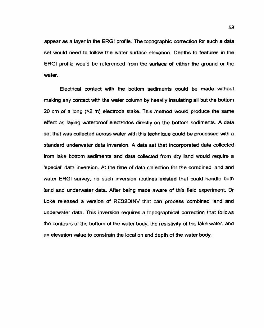
appear as a layer in the ERG1 profile. The topographic correction for such a data
set would need to follow the water surface elevation. Depths to features in the
ERG1 profile would be referenced from the surface of either the ground or the
water.
Electrical contact with the bottom sediments could be made without
making any contact with the water column by heavily insulating all but the bottom
20 cm of a long (>2 rn) electrode stake. This method would produce the same
effect as laying waterproof electrodes directly on the bottom sediments. A data
set that was collected across water with this technique could be processed with a
standard underwater data inversion. A data set that incorporated data collected
from lake bottom sediments and data collected from dry land would require a
'special' data inversion. At the time of data collection for the combined land and
water ERG1 survey, no such inversion routines existed that could handle both
land and undenvater data. After being made aware of this field experiment. Dr
Loke released a version of RES2DINV that can process combined land and
underwater data. This inversion requires a topographical correction that follows
the contours of the bottom of the water body, the resistivity of the lake water, and
an elevation value to constrain the location and depth of the water body.
Open Sand ~n Open Water
Wooded Levees
1 I 1 I I 1 I I I I I t 0 1 GO 200 300 400 500 600
Drstance along survey line BTC301 (rn)
Figure 18 Topographic profile of ERG1 suwey BTC307. The water surface in the wetland is higher than the surface of the abandoned Beavertail Channel. Elevation in this figure is relative to an arbitrary datum.
Even if all the data collection problems with the combined land and water
ERG1 survey were corrected. the data set could not be processed with the new
combined land and water data inversion- Survey line BTC3Ol includes two water
bodies with different surface elevations and water character (resistivity). Survey
line BTC301 also includes several locations that are lower than the water surface
that are not underwater (Figure 18). Dr. Loke intends to incorporate horizontal
constraints for the location of water bodies in a future release of RES2DINV
(pers. comm., 2000).
7.2. Electrode Array Field Experiment
Although a great deal of literature exists that describes the sensitivity,
depth of investigation, resolution, and susceptibility to noise of the three
commonly used electrode arrays for ERG1 (Wenner, Wenner-Schlumberger, and
dipole-dipole), each researcher appears to have their own favorite (Ward, 1990;
Reynolds, 1997; Dahlin and Loke, 1998; Loke, 1999).
The goal of this field experiment was to determine the best array for
imaging buried mudencased sand channel-fills and crevasse-splay sheet sands.
Because this experiment was carried out at almost all of the survey sites. there is
too much data to present here. For the sake of brevity, only the Wenner array
and the dipole-dipole array from two representative cases, the Beavertail
channel-fill (BTC102 and BTC103) and the Schoonrewoerd channel-fill and
braid-plain (NL9309101 and NL9309103), are presented.
7.2.1. Methods for this Field Experiment
In general, this field experiment involved collecting three data sets on
each survey line: one with a Wenner array, one with a Wenner-Schlumberger
array, and one with a dipole-dipole array. The equipment was not moved
between each series of measurements. The data sets were assessed by
qualitatively comparing their associated ERG1 profiles.
Quantitative comparison was not possible because there is no method to
determine the difference between an ERG1 profile and the subsurface. The
percent RMS (root mean square) error included with the ERG1 profile by the
inversion software can not be used for quantitative comparisons because it is a
measure of the fit between the model and the data and has nothing to do with the
relationship between either the model or the data and the 'real world'.
The data from the Beavertail channel-fill was collected using a Wenner
array followed by a dipole-dipole array on a 56 electrode survey line with a 1 m
electrode spacing. The survey was 55 long and was designed to collect
information up to 12 m deep. To keep all the ERG1 surveys across the Beavertail
channel-fill comparable, the first electrode for BTC102 and BTC103 was located
at meter 82 along the survey line. The data from the Schoonrewoerd channel-fill
was collected using a dipole-dipole array followed by a Wenner array on a 21
electrode survey line with a 10 rn electrode spacing. The survey was 200 rn long
and was designed to collect information from up to 32 m deep.
A preliminary assessment of the array test results indicates that for some
surveys the ERG1 profile from the Wenner array data was much cleaner, clearer.
and easier to interpret than the ERG1 profile from the dipole-dipole data
(e.g. Figure 19). For other surveys, the ERG1 profile from the Wenner array data
was very similar to the ERG1 profile from the dipole-dipole array data (e.g. Figure
20).
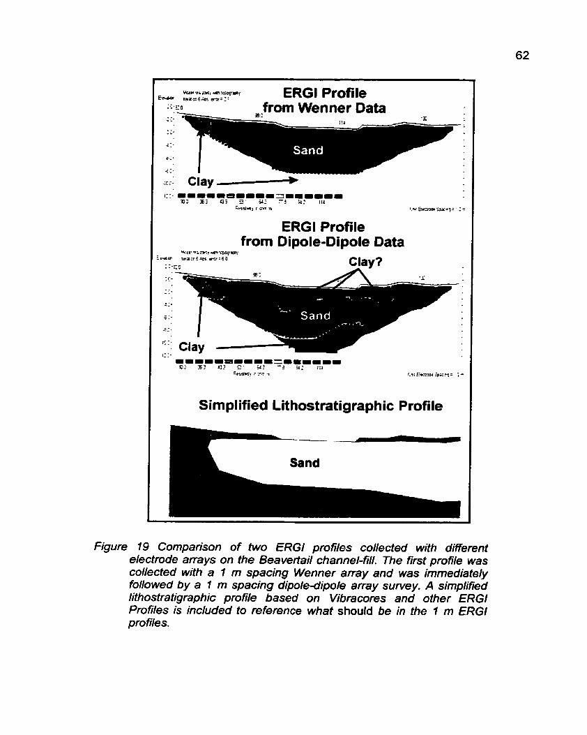
62
~ c H r ? i . t".ly & !-I csatai& mu=:'
- - ERG1 Profile
* .- . -- -a from Wenner Data -.-. . - 'I
-. . . - - 2:.
- - C c '
. - < - -
.;cI: Clay - I::. m m r r r , e a ~ ~ ~ ~ m ~ = r r r
3 3 E: 4? J: 8 2 Ill ;*ruw, r .irn TI I . l r ~ ~ u r ; = ':z
ERG1 Profile
%ecq ?t.'n, .m.ccc+~wrr from Dipole-Dipole Data
E t d m :f,sie:re~ ',TJ'F;O
---c:
- - C .' - -
CC'
- , = n m m = ~ . - ~ - m q 4 = = m r = = z, I: O.' - 9: 4 I::
'famra, r :-ir n r.a: =lcCPf~ :ox?; = ; T
Simplified Lithostratigraphic Profile
Figure 19 Comparison of two ERGI profiles collected with different electrode arrays on the Beavertail channel-fill. The first profile was collected with a I m spacing Wenner array and was immediately followed by a 1 rn spacing dipole-dipole array survey. A simplified lithostratigraphic profile based on Vibracores and other ERG1 Profiles is included to reference what should be in the I m ERGI profiles.

ERG1 Profile from Dipole-Dipole Data I e c l h t u l o ? abs trmr = %
C 0 so KO 13 183 m
:: 3: I
1ne.s~ Uodd =esalhfly S c m n
m m m o m m m m m m 100 7 2 ' ! 4 5 7:: I : 3 9 4 3213
Eeslstntf rn f m m '-16 aearcd? :pacing IC C m
ERG1 Profile from Wenner Data m
4 3 : :' 3 :
I W T ~ Uodtl =esstnrtf Eec:lan
m m m m m m m E l m m m m m m IJQ 7:' 1 4 6 1; 7 1 9 Z ' d 389
i;as~stmtf m ~ t m m -nn elerlnda spacog IC 6 m
Simplified Lithostratigraphic Profile
Figure 20 Comparison of two ERGl profiles collected with different electrode arrays on the Schoonrewoerd channel-fill and braidplain. The first profile was collected with 10 m spacing dipoledipole array and was immediately followed by a 10 m spacing Wenner array survey. A simplified lithostratigraphic profile based on hand cores (Makaske. 1998) is included to reference what should be in the 10 m ERGl profiles.

After numerous array tests it became apparent that if the dipoledipole
array data was collected before the Wenner array data (e.g. Figure 20), the ERG1
profiles were very similar. If the dipole-dipole array data was collected after the
Wenner array data (e-g. Figure 19). the ERG1 profiles were considerably
different.
The results of the electrode array field experiment indicate that the timing
of data collection affects the results of the electrode array comparisons, which
implies that repeating measurements on a suwey line somehow alters the
electrical behavior of the subsurface or the interface between the electrode
stakes and the subsurface. Given an awareness of the temporal signal, the array
test results suggest that the Wenner array provides a better ERG1 profile than the
dipole-dipole array (Figure 21).
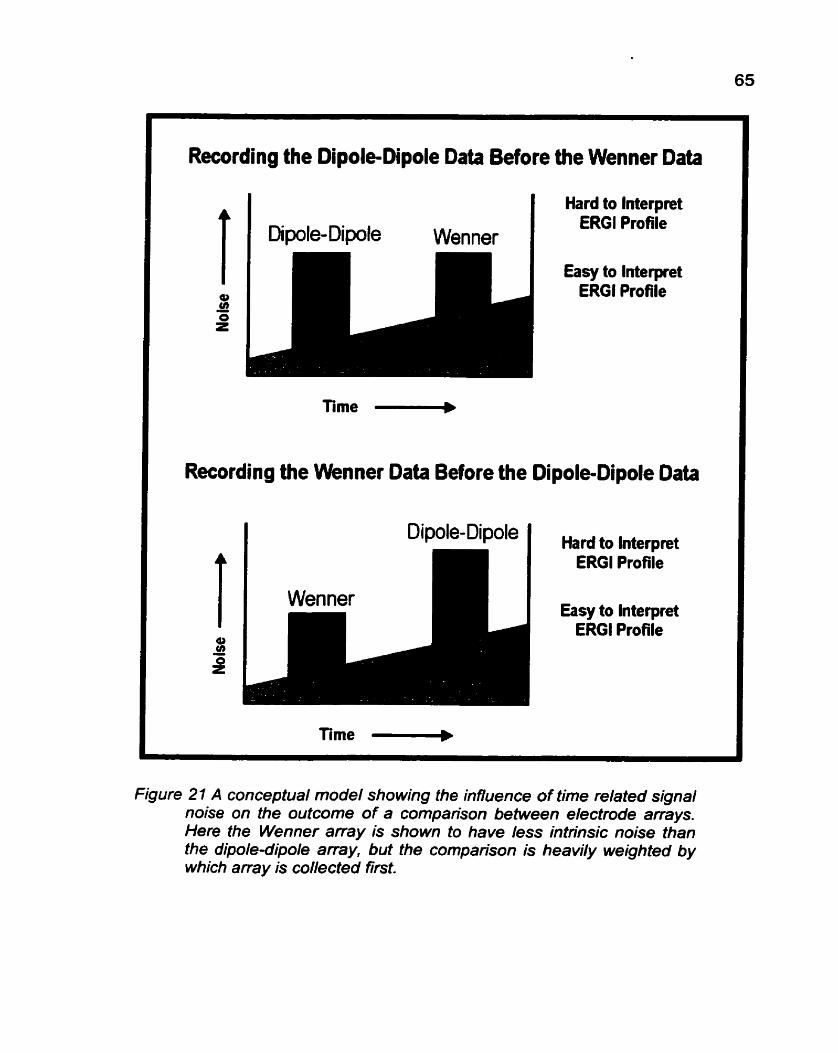
1 Recording the Dipole-Dipole Data Before the Wenner Data
T Hard to lnterpret
ERG1 Profile
Easy to lnterpret aa U )
ERG1 Profile - 0 Z
Time #-+
Recording the Wenner Data Before the Dipole-Dipole Data
Hard to Interpret
T ERG1 Profile
Easy to Interpret
aa ERG1 Profile
cn - P
Time 1-b
Figure 21 A conceptual model showing the intluence of time related signal noise on the outcome of a comparison between electrode anays. Here the Wenner array is shown to have less intrinsic noise than the dipole-dipole array, but the comparison is heavily weighted by which array is collected first.

7.3.Cumulative Electrode Charge-Up Effect Field
Experiment
Back-to-back repeated surveys on the same survey line appear to lead to
poorer and poorer quality ERG1 profiles. This problem has not been previously
reported. A possible cause for the decrease in profile quality is increasingly noisy
data due to 'cumulative electrode charge-up effects'.
Electrode charge-up is thought to occur at the interface where electrical
current passes from the electrode stakes into the ground (Dahlin, 2000).
Although nothing physically passes through this interface, electrical current is
transferred across it. The current is transferred across the interface by a build-up
(or deficit) of free electrons in the electrode stake and a corresponding build-up
of positive (or negative) ions in the pore fluids in the ground surrounding the
electrode stake. As the current flows, the build-up increases and eventually gets
large enough to produce a non-linear increase in the resistance of the circuit and
results in erroneous apparent resistivity measurements (Dahlin, 2000).
ERG1 data collection is designed to avoid charge-up effects. Resistivity
measurement equipment involves four electrodes to avoid immediate electrode
charge-up during current transmission ovenvhelming the voltage measurement.
Each apparent resistivity measurement recorded into a data set is actually the
average of a series of measurements with opposite polarity. This minimizes noise
while avoiding short-term electrode charge-up effects. The set of resistivity
measurements for an ERG1 profile is collected in a pattern that avoids using a
current electrode (A or 9) as a potential electrode (M or N) for as long as
possible in an effort to eliminate mid-term electrode charge-up effects
(M. Langmanson, pers comm., 2000).
Long-term subtle effects of electrode charge-up are unknown. This field
experiment was conducted to assess long-term cumulative electrode charge-up
at a site with a collection of unnamed buried paleochannels near the Lek River,
approximately 14 km east of Rotterdam, the Netherlands (surveys CSOlOl
through CS0108).
7.3.1. Methods for this Field Experiment
Data for the cumulative electrode charge-up effects field investigation was
collected on a 28 electrode survey line with a 5 rn electrode spacing. The survey
was 275 m long and was designed to collect information from up to 43 m deep.
Seventeen data sets were collected without moving the data collection
equipment (Figure 22); 9 electrical contact resistance tests, 4 Wenner array
surveys, and 4 Wenner-Schlumberger array surveys. A contact test was run
before any other data collection. A contact test was the collected after each of
the other measurements. The Wenner and Wenner-Schlumberger surveys were
alternated. The electrical contact resistance tests were designated R1 through
R9. The Wenner array surveys were designated Wl through W4. The Wenner-
Schlumberger array surveys were designated S1 through S4.
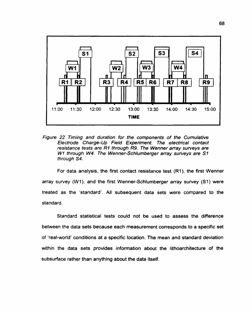
11:OO 11:30 12:OO 12:30 13:OO 13:30 14:OO 14:30 15:OO
TIME .
Figure 22 Timing and duration for the components of the Cumulative Electrode Charge-Up Field Experiment. The electrical contact resistance tests are R 7 through R9. The Wenner array surveys are W I through W4. The Wenner-Schlumberger array surveys are SI through S4.
For data analysis, the first contact resistance test (Rl), the first Wenner
anay survey (W1 ), and the first Wenner-Schlumberger array survey (S1) were
treated as the 'standard'. All subsequent data sets were compared to the
standard.
Standard statistical tests could not be used to assess the difference
between the data sets because each measurement corresponds to a specific set
of 'real-world' conditions at a specific location. The mean and standard deviation
within the data sets provides information about the lithoarchitecture of the
subsurface rather than anything about the data itself.

If the subsurface conditions remain constant and the measurement
process does not change, repeat data sets should have identical data rather than
just identical means and standard deviations. The goal of this field investigation
was to determine if the measurement process was altering conditions sufficiently
that repeat data sets are not identical.
A simple tool to test for and assess the difference between repeat data
sets is to examine the 'bias' between individual measurements (e.g. W l i - W2i:
Bland and Altman, 1983; 1986; Pollock et al, 1992). A second technique used to
assess differences between data sets is Passing-Bablok regression analysis.
The Passing-Bablok method can handle data that is not normally distributed and
that has error on both axes. Because of this, it is capable of detecting very small
differences between 'real world' data sets (Passing and Bablok, 1983; Payne,
1997).
Statistical comparison of the data sets was run using Microsoft@ Excel
2000 and Analyze-Itm. Although Analyze-Itm is a macro for Excel; it does not
use Excel's flawed statistical functions (see McCullough, 1998; 1999).
A comparison between the repeat ERG1 surveys was made on the % RMS
fit for the third iteration of data inversion to assess the influence of any
differences between the repeat data sets on the subsequent ERG1 profiles.
The bias between W1 and W2 was examined in .detail. An assessment
was made to determine if the distribution of bias between individual apparent
resistivity measurements (Wli - W2i) had any relationship with the two key -
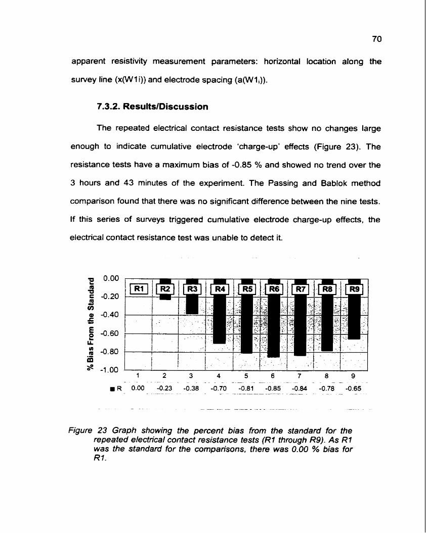
apparent resistivity measurement parameters: horizontal location along the
survey line (x(W 1 i)) and electrode spacing (a(W 1 i)).
The repeated electrical contact resistance tests show no changes large
enough to indicate cumulative electrode 'charge-up' effects (Figure 23). The
resistance tests have a maximum bias of -0.85 % and showed no trend over the
3 hours and 43 minutes of the experiment. The Passing and Bablok method
comparison found that there was no significant difference between the nine tests.
If this series of surveys triggered cumulative electrode charge-up effects, the
electrical contact resistance test was unable to detect it.
Figure 23 Graph showing the percent bias from the standard for the repeated electrical contact resistance tests (R 1 through R9). As R 1 was the standard for the comparisons, there was 0.00 % bias for R1.
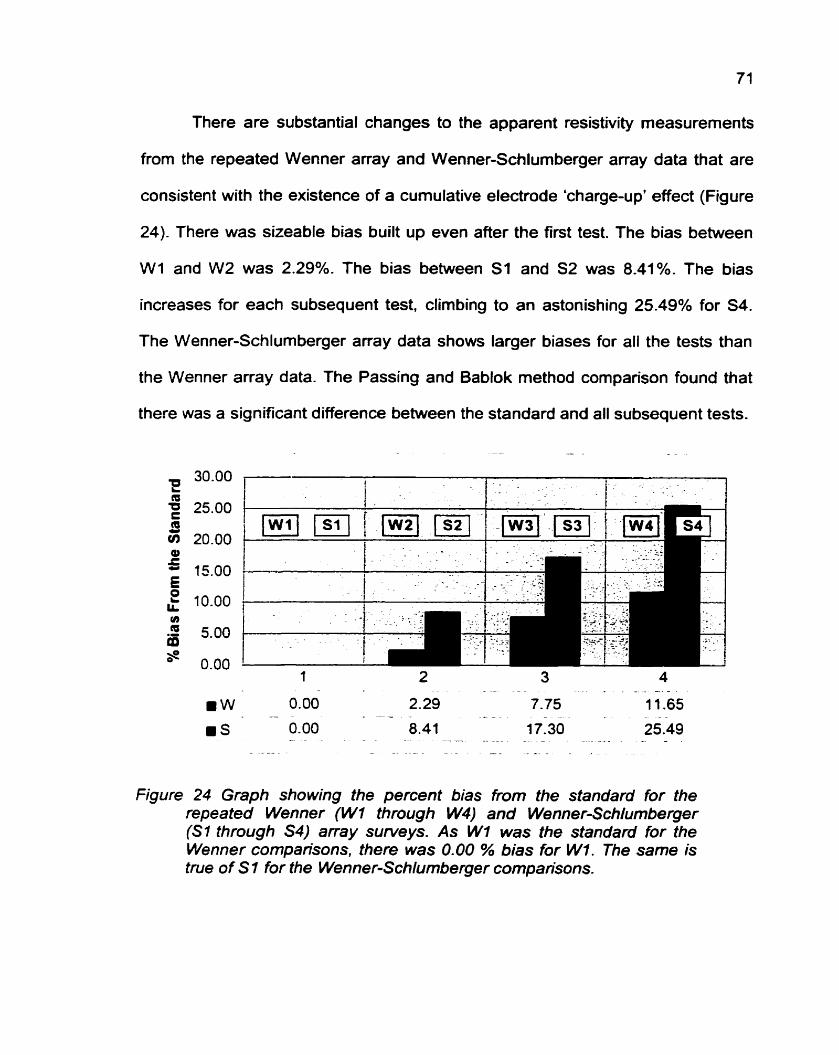
There are substantial changes to the apparent resistivity measurements
from the repeated Wenner array and Wenner-Schlumberger array data that are
consistent with the existence of a cumulative electrode 'charge-up' effect (Figure
24). There was sizeable bias built up even after the first test. The bias between
W1 and W2 was 2.29%. The bias between S1 and S2 was 8.41%. The bias
increases for each subsequent test, climbing to an astonishing 25.49% for S4.
The Wenner-Schlumberger array data shows larger biases for all the tests than
the Wenner array data. The Passing and Bablok method comparison found that
there was a significant difference between the standard and all subsequent tests.
Figure 24 Graph showing the percent bias from the standard for the repeated Wenner (W1 through W4) and Wenner-Schlumberger (Sf through S4) array surveys. As W1 was the standard for the Wenner comparisons, there was 0.00 % bias for W1. The same is true of S 1 for the Wenner-Schlumberger compansons.

These results do not prove the existence of long term subtle electrode
charge-up effects. However, the fact that repeated surveys do not produce
identical data sets and that the difference between the data sets increases with
the number of repeats, proves that some factor, such as electrode charge-up,
was definitely having a deleterious effect on the data.
Decreasing data quality intuitively leads to higher % RMS model fit (poorer
fit) for the corresponding ERG1 profiles. This assumption holds true for the data
sets collected for the cumulative electrode charge-up experiment (Figure 25)-
The % RMS model fit increased from 0.9 % to 16.8 % over the four Wenner array
ERG1 profiles and from 2.4 % to 21.2 % over the four Wenner-Schlumberger
array ERG1 profiles. The increase in % RMS model fit for the repeated surveys
reflects the decreasing quality of the data and indicates that it was procedurally
incorrect to qualitatively compare ERG1 profiles from repeated surveys on the
same suwey line.
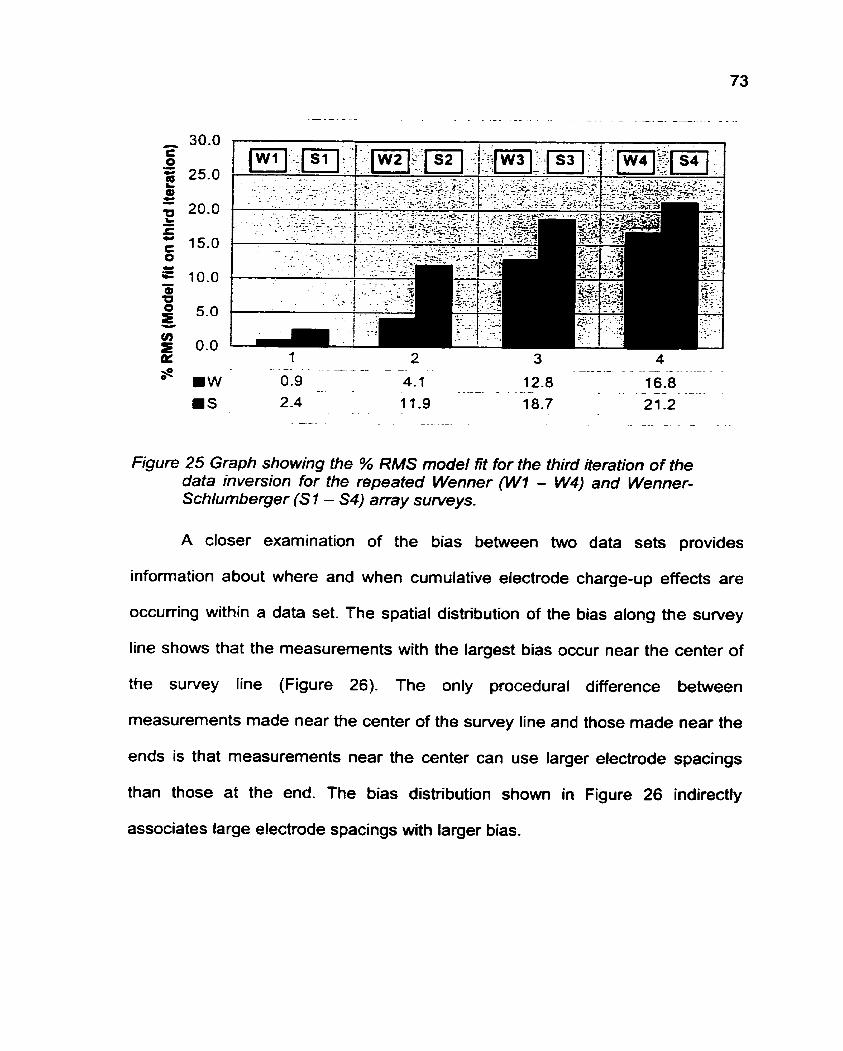
Figure 25 Graph showing the % RMS model fit for the third iteration of the data inversion for the repeated Wenner (W7 - W4) and Wenner- Schlumberger (S 1 - S4) array surveys.
A closer examination of the bias between two data sets provides
information about where and when cumulative electrode charge-up effects are
occurring within a data set. The spatial distribution of the bias along the survey
line shows that the measurements with the largest bias occur near the center of
the survey line (Figure 26). The only procedural difference between
measurements made near the center of the survey line and those made near the
ends is that measurements near the center can use larger electrode spacings
than those at the end. The bias distribution shown in Figure 26 indirectly
associates large electrode spacings with larger bias.
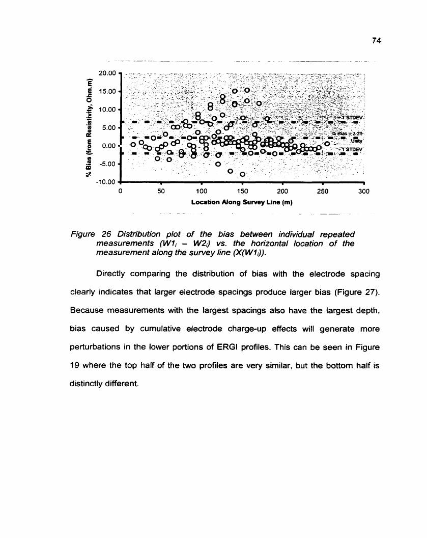
Location Along Survey Line (m)
Figure 26 Distribution plot of the bias between individual repeated measurements (Wli - W2i) vs. the horizontal location of the measurement along the suwey line (X(W7i)).
Directly comparing the distribution of bias with the electrode spacing
clearly indicates that larger electrode spacings produce larger bias (Figure 27).
Because measurements with the largest spacings also have the largest depth.
bias caused by cumulative electrode charge-up effects will generate more
perturbations in the lower portions of ERG1 profiles. This can be seen in Figure
19 where the top half of the two profiles are very similar, but the bottom half is
distinctly different.

A-Space for Wenner Array (m) --
Figure 27 Distribution plot of the bias between individual repeated measurements (W7i - W2i) vs. the electrode spacing (a(W1i)) of the measurement.
The results from the cumulative electrode charge-up experiment prove
that long-term charge-up effects lead to decreasing data quality and decreasing
ERG1 profile quality even after only one repeated survey on the same survey line.
The cumulative electrode charge-up effects are greatest for large electrode
spacings and manifest themselves in the lower portion of later ERG1 profiles.
Further study is required to determine how long a 'resting' period must be
observed to be sure that conditions have 'reset' between repeat surveys so that
investigations testing different arrays, different electrode stakes, different
instrument settings, et cetera can be completed without cumulative electrode
charge-up effects.

CHAPTER 8. CONCLUSIONS
ERG1 profiles accurately portray lithology, stratigraphy, and geometry of
buried sand and gravel fluvial deposits. Variations in the modeled resistivity
values represent different lithologies. Geometries of homogeneous deposits are
represented by zones of similar resistivity values. For example, mud-encased
sand-filled channels appear as channel-shaped high resistivity anomalies.
Vibracores confirm that such anomalies correctly represent the lithology and
geometry of the 'real-world'.
Methodology refinements suggested by this thesis make ERG1 field work
simpler and more reliable. Future improvements to the equipment and software
are expected to solve some of the problems with ERG1 investigations in fluvial
environments. One problem is the decrease in data quality associated with
repeated surveys on the same survey line, possibly caused by cumulative
electrode charge up effects. This inability to collect repeat data sets restricts
researcher's efforts to assess different data collection techniques or instrument
settings. Further work is suggested to better understand and mitigate this
problem. The problem of dry or frozen sediments will likely remain unresolved.
Dry or frozen sediments lack a camer for the electrical current used during
resistivity measurement and can not be studied using ERGI.
The field experiments in this thesis indicate that ERG1 is a remarkable
geophysical tool. It detects complex lithofacies changes and maps geometries. It
functions equally well in conductive sediments (silt-clay, organic, brackish, or
saline) and in resistive sediments (sand, gravel, or peat). This means that ERG1
can detect and delineate resistive bodies buried in conductive sediments. ERG1
is going to be the next shallow geophysical revolution for investigating fluvial and
other Quaternary-aged depositional successions.
Remember: Resistance is not futile!

REFERENCES
Abbado, D., and Filgueira-Rivera, M., 2000. High Resolution DGPS Long Profile of the Anastomosed Reach of the Columbia River, British Columbia, Canada, Unpublished Data, University of Nebraska.
Abdul Nassir, S.S., toke. M.H., Lee, C.Y, and Nawawi, M.N.M., 2000. Salt Water Intrusion Mapping by Geoelectrical lmaging Surveys, Geophysical Prospecting, 48, 547-66 1.
Archie, G.E., 1942. The Electrical Resistivity Log as an Aid to Determining Some Reservoir Characteristics. Transactions of the American Institute of Mining, Metallurgical, and Petroleum Engineers, 164, 389-409.
Barker, R.D.. 1 989. Depth of Investigation of Collinear Symmetrical Four Electrode Arrays, Geophysics, 54, 8, 1031 -1 037.
Barker, R.D., 1992. A Simple Algorithm for Electrical lmaging of the Subsurface, First Break, 10. 2, 53-62.
Beard, L.P., Hohmann, G.W., and Tripp, A.C., 1996. Fast ResistivityIlP Inversion Using A Low-Contrast Approximation, Geophysics, 6 1, 1, 1 69-1 79.
Berendsen, H.J.A., 1994, Handleiding: Voor Fysisch Geografisch Veldwerk in het Laagland Negende Druk, Vakgroep Fysische Geografie, Universiteit Utrecht.
Berendsen, H.J.A., 1998. Bird's-Eye View of the Rhine-Meuse Delta (The Netherlands), Journal of Coastal Research, 14,3, 740-752.
Berendsen, H.J.A., and Stouthamer, E., 2000. Late Weichselian and Holocene Paleogeography of the Rhine-Meuse Delta, The Netherlands, Paleogeography. Paleoclimatology, Paleoecology, 161. 31 1 -335.
Bland, J.M., and Altrnan, D.G., 1983. Measurement in Medicine: The Analysis of Method Comparison Studies, Statistician, 32, 301-31 7.
Bland, J .M., and Altman, D.G., 1986. Statistical Methods for Assessing Agreement Between Two Methods of Clinical Measurement, The Lancet, 307-31 0.
Broughton Edge, A.B., and Laby, T.H., 1931. The Principles and Practice of Geophysical Prospecting: The Report of the Imperial Geophysical Experimental Survey. Cambridge University Press, Cambridge.
Burger, H.R., 1992. Electrical Resistivity, Chapter 5 in: Exploration Geophysics of the Shallow Subsurface, Prentice Hall, New Jersey, 241 -31 6.
Chang, R., 1991. Electrochemistry, Chapter 19 in: Chemistry, McGraw-Hill, New YO&, 779-81 8.
Christensen, N.B., 2000. Difficulties in Determining Electrical Anisotropy in Subsurface Investigations, Geophysical Prospecting, 48, 1 -1 9.
Dahlin, T., 1996. 2D Resistivity Surveying for Environmental and Engineering Applications, first Break, 14, 7, 275-283.
Dahlin, T., 2000. Short Note on Electrode Charge Up Effects in DC Resistivity Data Acquisition Using Multielectrode Arrays, Geophysical Prospecting, 48, 181 -1 87.
Dahlin, T., and Loke, M.H., 1998. Resolution of 2D Wenner Resistivity lmaging as Assessed by Numerical Modeling, Journal of Applied Geophysics, 38, 237-249.
Dahlin, T. and Owen, R., 1998. Geophysical Investigations of Alluvial Aquifers in Zimbabwe, Proceedings: 4m European Environmental and Engineering Geophysics Society Meeting, Barcelona, Spain, 14-1 7 September 1998.
Daily, W. and Ramiret, A.L., 2000. Electrical lmaging of Engineered Hydraulic Barriers, Geophysics, 65, 1, 83-94.
Dey, A., and Morrison. H.F., 1979. Resistivity Modeling for Arbitrarily Shaped Three-Dimensional Structures, Geophysics, 34.61 5-632.
Edwards, L.S., 1977. A modified Pseudosection for Resistivity and IP, Geophysics, 42, 5, 1020-1 036.
El-Behiry, M.G. and Hanafy, S.M., 2000. Geophysical Surveys to Map the Vertical Extension of a Sinkhole: a Comparison Study, Proceedings of the Symposium on the Application of Geophysics to Engineering and Environmental Problems, February 20-24, Arlington, Virginia.
El-Hussain, I., Holbrook, J. and Sneed, C., 2000. Integrating Geophysical and Geological Methods to Delineate Buried Paleochannels in the New Madrid Seismic Zone of southeastern Missouri, Proceedings of the Symposium on the Application of Geophysics to Engineering and Environmental Problems, February 20-24, Arlington, Virginia.
Federal Geodetic Control Subcommittee and GPS Interagency Advisory Council, 2000. Comparison of Positions With and Without Selective Availability: Full 24 Hour Data Sets, Retrieved May 28, 2001 from the World Wide Web: htt~://www.ngs.noaa .aov/FGCS/info/sans SA/com~are/ERlA. htm
Gettys, W.E., Keller, F.J., and Skove, M.J., 1989. Current and Resistance, Chapter 24 in Physics, McGraw-Hill Book Company, New Yo*.
Gilson, E.W., Nimeck, G., Bauman, P.D. and Kellett, R., 2000. Groundwater Exploration in Prairie Environments, Proceedings of the Symposium on the Application of Geophysics to Engineering and Environmental Problems, February 20-24, Arlington, Virginia.

Gilvear, D., Winterbottom, S., and Sichingabula, H., 2000. Character of Channel Planforrn Change and Meander Development: Luagwa River, Zambia. Earth Science Processes and Landforms, 25,421 -436.
Geological Survey of Canada (1972). Map 1326A; geology; Lardeau (east half), British Columbia; scale 1 :50,000. Ottawa: Geological Survey of Canada.
Geological Survey of Canada (1979a). Map 1501A; geology; McMurdo (east half), British Columbia; scale 1:50,000. Ottawa: Geological Survey of Canada.
Geological Survey of Canada (1 979b), Map 1 502A; geology; McMurdo (west half). British Columbia; scale 1:50,000. Ottawa: Geological Survey of Canada.
Geological Survey of Canada (1 980). Diagrammatic structure sections (. . .) to accompany Map 1501A. McMurdo (east half) and Map 1502A. McMurdo (west half), scale 1 :50.000. Ottawa: Geological Survey of Canada.
Griffiths, D.H., Turnbull, J., and Olayinka, A.I., 1990. Two-dimensional Resistivity Mapping with a Computer Controlled Array, First Break, 8, 4, 121-129.
Hawood, K., and Brown, A.G., 1993. Fluvial Processes in a Forested Anastomosing River: Flood Partitioning and changing Flow Patterns, Earth Surface Processes and Landforms, 18, 749-751.
Hazen, M.E., 1990. Fundamentals of DC and AC Circuits, Saunders College Publishing, New York.
Heritage, G.L.. and Broadhurst, L.J., 1998. Modeling Stage-Discharge Relationships in Anastomosed Bedrock-Influenced sections of the Sabie River System, Earth Surface Processes and Landforms, 23,455465.
Knighton, A.D.. and Nanson, G.C., 1993. Anastomosis and the Continuum of Channel Pattern. Earth Surface Processes and Landforms, 18. 61 3-625.
Kunetz. G., 1966. Principles of Direct Current Resistivity Prospecting, Geoexploration Monographs, Ill.
Leopold, L.B.1 Wolman, M.G., and Miller, J.P., 1964. Fluvial Processes in Geomorphology, W.H. Freeman and Company, San Francisco.
Locking, T., 1983. Hydrology and Sediment Transport in an Anastomosing Reach of the Upper Columbia River, B.C., Unpublished Masters Thesis, University of Calgary, 1 07 p.
Loke. M.H., 1999. Electrical Imaging Surveys for Environmental and Engineering Studies: A Practical Guide to 2D and 30 Surveys. Unpublished Short Training Coarse Lecture Notes, Universiti Sains Malaysia, Penang, Malaysia.
Loke, M.H., 2000. RESZDINV Software User's Manual (version 3.44)
Loke, M.H. and Barker, R.D., 1996. Rapid Least Squares Inversion of apparent Resistivity Pseudosections by a Quasi-Newtonian Method, Geophysical Prospecting, 44, 1 31 -1 52.
Maillol, J.M.; Ortega-Ramirez, J.; Bandy, W.L.; and Valiente-Banuet, A., 2000. Contribution of Electrical Resistivity Methods to Paleoenvironmental Reconstruction and Groundwater Exploration in the Chihuahua Desert, Mexico, Proceedings of the Symposium on the Application of Geophysics to Engineering and Environmental Problems, February 20-24, Arlington, Virginia.
Maillol, J.M., Seguin, M.K., Gupta, O.P., Akhauri, H.M., and Sen, N., 1999. Electrical Resistivity Tomography Survey for Delineating Uncharted Mine Galleries in West Bengal India, Geophysical Prospecting, 47, 103-1 16.
Makaske, B.. 1998. Anastomosing Riven: Forms. Processes, and Sediments, Utrecht: Koninklijk Nederlands Aardrijkskuncfig Genootschap/Faculteit Ruimtelijke Weteschappen, Universiteit Utrecht (Nederlandse Geografische Studies 249).
McCullough, B.D., 1998. Assessing the Reliability of Statistical Software: Part I, The American Statistician, 52, 4, 358-366.
McCullough, B.D., 1999. Assessing the Reliability of Statistical Software: Part II, The American Statistician, 53, 2, 149-1 59.
Miall, A.D., 1996. The Geology of Fluvial Deposits: Sedimentary Facies, Basin Analysis, and Petroleum Geology, Springer-Verlag, New York.
Moorman, B.J., 1990. Delineation of LiUlofacies using GPR, Unpublished Masters Thesis, University of Calgary.
Passing, H. and Bablok, W., 1983. A New Biornetrical Procedure for Testing the Equality of Measurements from Two Different Analytical Methods: Application of Linear Regression Procedures for Method Comparison Studies in Clinical Chemistry, Journal of Clinical Chemistry and Clinical Biochemistry, 21, 709-720.
Payne, R.B., 1997. Method Comparison: Evaluation of Least Squares, Deming, and PassingIBablok Regression Procedures Using Computer Simulation, Annals of Clinical Biochemistry, 34, 31 9-320.
Pollock, M.A., Jefferson, S.G., Kane, J.W., Lomax, K., MacKinnon, G., and Winnard, C.B., 1992. Method Comparison - A Different Approach, Annals of Clinical Biochemistry, 29, 556-560.
Quinn, A., 1982. Crevasse Splay Deposits: A Study of the Geomorphology and Sedirnentology in an Anastomosing Fluvial Systems, Unpublished Masters Thesis, University of Calgary, 167 p
Reynolds, J.M., 1 997. An Introduction to Applied and Environmental Geophysics, John Wiley and Sons, New York.
Ritz, M., Robain, H., Pervago, E., Albouy, Y., Carnerlynck, C., Descloitres, M., and Mariko, A., 1999. Improvement to Resistivity Pseudosedion Modeling by Removal of Near Surface Inhomogeneity Effects: Application to a Soil System in South Cameroon, Geophysical Prospecting, 47, 85-1 01.
Roy, A. and Apparoa, A., 1971. Depth of Investigation in Direct Current Methods, Geophysics, 36, 5, 943-959.
Schumm, S.A., Eskine, W.D-, and Tilleard, J.W., 1996. Morphology, Hydrology, and Evolution of the Anastornosing Ovens and King Rivers, Victoria, Australia, GSA Bulletin, 108, 10, 121 2-1224.
Smith, D.G., 1972. Aggradation and Channel Patterns of the Alexandra-North Saskatchewan River, Banff National Park, Alberta, Canada, in: 0. Slaymaker and H. McPherson ed., Mountain Geomorphology, Tantalus Research, Vancouver.
Smith, D.G., 1983a. Anastornosed Fluvial Deposits: Modem Examples from Western Canada, Special Publications International Association of Sedimentologists, 6, 155-1 68.
Smith, D.G., 1983b. Vibracoring Fluvial and Deltaic Sediments: Tips on Improving Penetration and Recovery, Journal of Sedimentary Petrology, 54,2,660-663.
Smith, D.G., 1986. Anastomosing river deposits, sedimentation rates and basin subsidence, Magdalena River, northwestern Colombia, South America, Sedimentary Geology, 46, 1 77-1 96.
Smith, D.G., 1992. Vibracoring: Recent Innovations, Journal of Paleolimnology, 7, 137-143.
Smith, D.G., 1998. Vibracoring: A New Method for Coring Deep Lakes, Paleogeography, Paleoclimatology, Paleoecology, 140, 433-440.
Smith, D.G. and Putnam, P.E., 1980. Anastomosed River Deposits: Modem and Ancient Examples in Alberta, Canada, Canadian Joumal of Earth Sciences, 17, 1396-1406.
Smith, D.G. and Smith N.D., 1980. Sedimentation in Anastomosed River Systems: Examples from Alluvial Valleys Near Banff, Alberta, Journal of Sedimentary Petrology, 50, 1, 01 57-0164.
Sting/Swift User's Manual ver 3.0.10 Feb 2001
Telford, W.M., Geldart, L.P., Sheriff, R.E., and Keys, D.A., 1990. Applied Geophysics, 2nd Edition, Cambridge University Press, Cambridge.
Tong, L. and Yang, C., 1990. Incorporation of Topography into Two-Dimensional Resistivity Inversion, Geophysics, 55, 3, 354-36 1 .
Tornqvist, T.E., 1993. Fluvial Sedimentary Geology and Chronology of the Holocene Rhine-Meuse Delta, The Netherlands, Utrecht: Koninklijk Nedertands Aardrijkskundig Genootschap/Faculteit Ruimtelijke Weteschappen, Universiteit Utrecht (Nederlandse Geografische Studies 166).
van Dijk, G.J., Berendsen, H.J.A., and Roeleveld, W., 1991. Holocene Water Level Development in the Netherlands River Area; implications for Sea- Level Reconstruction, Geologie en Mijnbouw, 70, 31 1-326.
Ward, S.H., 1990. Resistivity and Induced Polarization Methods, in S.H. Ward ed., Geotechnical and Environmental Geophysics, Volume 1, 147-1 90.
Wolfe, P.J., Richard, B.H., Hauser, E.C. and Hicks, J.D., 2000. Identifying Potential Collapse Zones under Highways, Proceedings of the Symposium on the Application of Geophysics to Engineering and Environmental Problems, February 20-24, Arlington, Virginia.

APPENDIX A. GUIDELINES FOR ERG1 SURVEYING
This appendix is intended as an easy to use reference that will provide a
researcher will all the basic information necessary to conduct an effective ERG1
surveying campaign. It is a combination of results from informal, inferential, and
anecdotal ERG1 methodology experiments, an extensive review of published and
unpublished research, and three years of dedicated experiential learning. The
material is presented in an informal tone and is organized into categories that
should prove relevant to a researcher in the field.
The two following appendixes should also be useful for researchers
conducting ERG1 surveys. Appendix B describes electrode arrays in more detail
than there was room for within chapter 4 and 5. Appendix C breaks the entire
ERG1 surveying process down into 12 easy to follow steps.
A. 1 ERG1 Site Selection
a Sediments of interest should have a high resistivity contrast. Often contrast
simply stems from a reasonable grain size difference (silt clay vs. sand
gravel). Subtle contrasts can be imaged i f there are no high contrast materials
in the survey to overwhelm the difference between the signals from the low
contrast materials.
Sediments image best if they are massive: without internal structure or
bedding. Although for most of our projects no real anisotropic problems will

occur, the method can not discern a difference between a mixture of sand and
mud and finely interbedded sand and mud.
a Lateral facies changes greatly enhance the clarity of the profiles and the ease
of interpretation. ERG1 is, as discussed here, a 2D method and there are
better methods to answer 1 D questions.
ERG1 profiles work best if there are no lateral facies changes to either side of
the survey line; try not to ask a 20 method to answer a 30 question.
a The water table will be displayed in ERG1 profiles. It is best to know in
advance the approximate depth of the water table so that it is not accidentally
interpreted as a lithofaues change.
a Low contact resistance (resistance between the electrode stake and the
ground) is critical to good data, so sites with moist conductive sediments at
the surface produce the best profiles. Although ERG1 data can be collected
with dry sand and gravel or scree at the surface, it's more work and produces
noisier data.
a Straight suweys produce the best data. Curves in the survey line violate the
assumptions in equation 5 resulting in erroneous resistiwty measurements. A
curve may actually generate a fallacious feature in the ERG1 profile similar to
a buried channel.
A.2 ERG1 Resolution and Depth of Investigation
Depth of penetration for an ERG1 measurement is not worth discussing
because it is for all practical purposes infinite.
a Depth of investigation is a term used in this thesis to describe the depth where
half of the electrical current flowing for an apparent resistivity measurement
flows above this depth and half flows below. All material above the depth of
investigation and a large amount of the material below the depth of
investigation contributes to the measurement.
Depth of investigation is approximately 115 of the survey line's total length.
Although formulas exist to calculate the exact depth of investigation for each
electrode array (Roy and Apparoa, 1971 ; Barker, 1989; Ward, 1 990), they are
only accurate for 100 % homogeneous materials.
Resolution of the ERG1 profiles is approximately 112 of the electrode spacing
(pers. comm., Loke, 1999). Resistivity measurements decrease in resolution
with depth, so we have to say either that the resolution or the mathematical
uncertainty of the ERG1 profiles increases with depth.
Depth of investigation and resolution are a trade-off dependant on the
electrode spacing and the total number of eledrodes. For example, 56
electrodes spaced 12 m apart measured with a Wenner electrode array
produces an ERG1 profile 110 m deep with 6 m resolution. Conversely, 56
electrodes spaced 2 m apart measured with a Wenner electrode array
produces an ERG1 profile 18.3 rn deep with 1 m resolution.
A.3 ERG/ Data improvement
Keep all connectors clean! Keep covers on connectors until they are in use.
Blow the connecters out with air to remove dust and debris every time you
connecting them. Every five or ten surveys blow the connectors out with
electrical contact cleaner.
a Clean the electrodes! Simply brushing the electrode with fine or medium steel
wool every other survey will result in a substantial decrease in noise.
a Inspect the edges of the platforms on the electrode stakes. All contact
between the electrode and the stake occurs on the inside edges of the top
and front of the electrode stake platform. If this edge becomes burred by
bashing against other stakes while in transport or by poor mallet technique
while driving the stakes into the ground, contact between the stake and the
electrode is substantially reduced and noisier data will result. A quick pass
with a file eliminates this problem.
a Do not wiggle the electrode stakes. Tripping on the cable, adjusting h e
electrode, rotating the electrode so you can see the number, etc alters and
most likely decreases the area of contact between the electrode stake and the
ground and noisier data w'll result. ALWAYS put the electrode on the stake

before inserting it into soft ground, this makes a HUGE difference to data
quality.
Placing slack cable to one side, laid out so that it does not loop or cross itself,
eliminates any chance of self-induced inductive noise in the cable. However, it
will get in your way and perhaps trip you (see above). A happy medium is to
spread it out as much as possible, but always to the same side of the survey
chain so that foot or vehicle travel along the survey is possible in a cable free
zone.
Less current means better data. Use the lowest possible amperage setting
that provides clean data to reduce charge-up effects, get much cleaner data,
and avoid INOVL errors. - Longer measurement cycles (see the Stingswift User Manual for details,
2001) improve the data. However, if you are doing everything else right, it will
be a negligible improvement. For regular surveys, use the shortest time cycle
to obtain the most data in the least time. For problem surveys, consider longer
cycles and bring a book.
Suweys should image around twice the depth of the target of interest. ERG1
profiles are much clearer and easier to interpret if the model has sufficient
data to 'resolve' the bottom and sides of features. - If at all possible, reduce your contact resistance. Keep it below 1 kn!
A.4 Electrical Contact Resistance
Contact resistance is a measure of how well electrical current can pass
from the electrode stakes into the ground. Often achieving and maintaining low
contact resistance is difficult and frustrating. However, a single electrode stake
with high contact resistance will produce 'striping' in the resistivity pseudo-
section. If several adjacent electrode stakes have high contact resistance, it may
lead to artificial features in the resultant ERG1 profile. Note that repeated contact
resistance tests may lead to 'charge-up effects' and noisy data.
The 'built-in' contact resistance test in AGl's Sting simply records the
electrical resistance between each electrode and it's neighbour. Because only
two electrodes are used for the measurement, it is not a resistivity measurement
and tells us very little about the sediment except for its ability to pass electrical
current to and from an electrode stake.
For the best data, contact resistance should be below 1 kR. Lower is
better. Other researchers have collected useful, albeit noisy, resistivity data at
MR's of contact resistance. At that level, only the coarsest interpretation would
be possible.
Often simply reinserting the eledrode into the ground in a new hole will
resolve the problem.
a Sometimes a half-liter of salt water is necessary to build up a 'bulb' of
conductive sediment around the stake. We've found pickling salt to be the
best value.
In particularly dry sediments, wetting the ground around the stake is not
enough. When crossing open sand on crevasse-splays we dug a shallow
trench (1 0 cm deep by 30 cm wide) along the entire survey line, covered the
base of the trench with salt, and poured copious water into the trench (10
liters/meter). We would leave the site overnight then follow standard salting
and wetting procedures to collect data the next day. Other researchers claim
to have used sponges saturated with salt solution or even saturated diapers to
increase the area of electrical contact (L. Langrnanson, pers. comm., 2000).
In loose materials, such as open matrix scree, other researchers have had
success using long electrode stakes (>2m of rebar) and large sponges at the
ground's surface to obtain reasonable contact resistance (D. Chapellier, pers.
comrn., 2000).
Highly electrically conductive sediments can have odd contact resistance
behavior a few hours after a hard rain. The deeper the electrode stakes
penetrate the ground, the more inconsistent the readings and the more errors
encountered. By resetting the stakes into the ground to about 5 cm of
penetration, problems may be avoided.
In frozen ground, we have had moderate success penetrating through to
unfrozen sediments by driving the stakes in a great depth. Other researchers
have had success using large (2.5 cm X 1.25 m) stainless steel electrode
stakes to obtain contact with frozen ground (G. Nimek, pers. comm., 2001)
a If you are considering ERG1 at a site, but are hesitant because the ground
appears too dry to get good contact, set up 2 to 4 electrodes right beside your
vehicle and do a contact resistance test. If the contact resistance is extremely
high for this 'quick and dirty' test, you'll know before you've spent an hour
setting up an entire survey that extraordinary measures would be necessary
to achieve sufficiently low contact resistance for the full line.
On long survey lines, use two-way radios to communicate between the
researcher running the contact test and the researcher troubleshooting the
electrodes and electrode stakes. This vastly speeds up the process of getting
a troublesome line into production.
A.5 Error Codes on the Sting
A setting on the Sting controls whether data collection stops on an error
code or not. For most surveys, it is better to miss some data due to an error than
to slow down production. However, contact resistance tests stop on errors.
Always chase down and solve errors that occur during a contact resistance test.
For a contact resistance test, if the Sting stops on an error, you can repeat
the failed measurement by pressing F1, or you can continue on to the next
measurement by pressing F2. The most efficient method is to record all errors.
continuing the test after each error, and trouble shoot the entire survey at once.

When you are ready to retry, set the test parameters to a few electrodes before
your problem and start the contact test over.
A.5.1 The HVOVL Error Code
The HVOVL error code (high voltage overload) means that the Sting can
not establish a current through the AB circuit. HVOVL errors are usually caused
by cable connection problems, by power problems, or by extreme electrical
contact resistance.
a You will get a HVOVL if the Sting's battery pack is low even if you are working
with an external battery!
You will get a HVOVL if the Swift is not turned on or if it shuts down due to low
power.
a You will get a HVOVL if you are requesting to use electrodes that are not
connected to the system (e.g. having electrodes 29-56 hooked up but the
control file asks for 1-28).
You will get a HVOVL if the cable or one of the electrodes is damaged and
communication is interrupted. This can be tested by moving the Sting and
Swift to the other end of the cable and determining which electrodes can be
'seen' from the other end.
a On rare occasions, this error shows up due to contact problems between an
electrode, its stake, and the ground. We've had these occur due to a piece of
grass being between the electrode and the stake.

A.5.2 The TXOVL Error Code
The TXOVL error code (transmitter overload) means that the signal
through the AB circuit (current) is fluctuating. You have variable contact
resistance in the A6 circuit. Unless there are large IP or SP effects going on.
simply treat as a contact resistance problem and solve it.
A.5.3 The INOVL Error Code
The INOVL error code (input overload) means that the input amplifier has
been overwhelmed by the signal through the MN circuit (measurement). In other
words, the voltage being measured is too high for the meter. Usually the Sting
automatically steps down the current, which subsequently drops the voltage and
solves the problem. If the Sting is unable to make a reading even after stepping
down the current, the INOVL error code is displayed.
If you are losing a great deal of data to lNOVt errors, consider reducing
the max current on the Sting: remember that less current leads to better
readings. Other possible solutions include resetting the problem electrode stakes
in new holes or resetting the entire survey with larger electrode spacing.
A. 6 General Improvements to ERG1 Field Operations
Don't use the cable shipping crates supplied by the equipment manufacturer
while in the field. Use smaller plastic boxes with one cable (14 electrodes) per
box. This makes cable wiling much faster. Any commercially available plastic
box is lighter than the shipping crates, and only having one cable per box

really increases their ease of mobility. Any commercially available plastic box
is more user friendly than the shipping crates because they don't have nasty
sharp metal corners that tear equipment and researchers.
Obtain a two-wheeled lawn cart to haul around the equipment in the field.
Coiling cable into a box on a cart is much easier on the researchers' backs
than leaning over all day and reduces the number of times the cable box must
be lifted.
Always take more rubber bands with you for attaching the electrodes to the
stakes than you think you could ever use. Nothing is more aggravating than
running out of rubber bands after spending many hours getting to a site and
spending most of an hour setting up a survey.. .
Use some form of survey flags, such as wire stake seismic flags, to mark off
the end of your survey chain and various points along the survey chain. This
makes setting up a straight survey much easier. It also makes locating the
ends of your survey simple if further investigation is required on a later date.
The most data in the least time can be gathered by first collecting a large
spacing survey. then collecting smaller spacing surveys over targets of
interest as shown in the preliminary survey. We prefer conducti-ng a 10 m, a
5 m. and then a 2 m survey at each location. Frequently the 10 m survey is
the only survey to cover the entire horizontal extent of the survey site.
a Avoid all livestock and in particular cattle! They find the resistivity gear very
interesting and quite tasty. A cow is quite capable of inflicting substantial
damage to the resistivity gear by simply having a chew or two or by stepping
on the cable.
A. 7 ERG1 Data Processing
a RESPDINV is simple to use and the manual (Loke, 2000) is excellent.
a The simplest way to obtain a clear and easy to understand ERG1 profile is to
'overparameterize the model'. Use the Thickness of Model Layer Increase
option to set the model layer thickness to 0.5 or 0.25 of the electrode spacing,
the layer thickness increase to 1 .O, and allow the number of model blocks to
exceed the number of data points. This vastly improves the apprent
resolution, but bemuse the data resolution has not improved,
overparamaterizing decreases the certainty of the ERG1 profile, particularly in
the lower portion of the profile.
Try all of the different settings and parameters available, but take good notes
so you can reproduce, and justify, your results.
a Often a slight modification to the contour intervals or the colors of your ERG1
profile will make interpretation much simpler. When comparing two or more
profiles, consider using the same contour intewals for all the profiles. This
may not be effective if the range of resistiwty values in the profiles varies
widely.
For buried mud-encased sand channel-fills and crevasse-splay sheet-sands
the HorizontaWertr'cal Flatness F i w the Limit Range of Model Resistivw,
the Reduce Effect of Side Blocks, the Use Robust Model Constraint, and the
Use Topographic Correction options typically produce the clearest ERG1
profiles.
Some ERG1 data sets lend themselves to processing with one dimensional
data inversion software. I D inversions typically define the resistivity of layers
and the thickness of the layers. This information is very useful for layered
sedimentary deposits and much better constrained than an ERG1 profile
produced by RES2DINV. However, any 2D sedimentary structures will turn a
1 D inversion into gibberish.
Software, such as RESIX2D by Interpex, inverts 2D resistivity data into bodies
with boundaries. This may be a better data inversion approach to investigate
buried mud-encased sand channel-fills and crevasse-splay sheet-sands than
the smooth cell-based approach used by RES2DINV.
A.8 AGl's Command Creator
Command Creator is the software AGI provides to produce command files
that control data collection on the StinglSwiff resistivity system. It is simple to
use and very helpful for visualizing the data collection process.
Note that Command Creator Version 1.2.1 has a 'bug' that doubles the
estimated depth of investigation for dipole-dipole surveys.
Note that Command Creator Version 1.2.1 has a 'bug' that keeps roll-along
files from having the correct horizontal location for the first electrode. For
example the first electrode on the first 14 electrode roll of a 2 m spacing
survey line is 28 meters from the start of the survey line, but Command
Creator will always set the first electrode position to zero. A simple way to
work around this problem is to set the X-location in the A m y Set-up option on
the Sting to the correct location for the first electrode.
A. 9 'Roll-Along ' Surveying for ERG1
a Rolling fewer electrodes maintains the greatest depth of data. If you are not
surveying to the maximum depth for an array, rolling more electrodes (28
instead of 14) may allow for a faster suwey with little loss of data. Look at all
options in command creator before making your decision.
Roll along surveys can be very time efficient if you disconnect the first cable
(e-g. q-14) as soon as it is out of use, but while measurements are still
occurring on the other cables (e.g. 1156). Use command creator to determine
which measurement is the last to use a particular electrode and after that
' measurement is collected, disconnect the cable and move it to it's location as
required by the next round of data collection.
Note that the command file for the fifth 14 electrode roll on a 56 electrode line
is the same command file as the first roll! Remember to change the X-location
for the first electrode though.. .
a Although data sets that contain many 'roll along's can slow down processing,
your only limitation to the size of your data set is time, computer memow, and
processing power. RES2DINVs set up program, Jambwin, can be set to
allow 2000 electrodes in one data set. The question becomes, what
information are you gaining from such a large and diff~cult to handle data set?
Could a larger spacing survey provide you with the outline you need then use
several 'point' surveys for more detail where necessary? Or is the situation 1 D
enough to use overlapping 1 D inversions?
APPENDIX B. UNDERSTANDING ELECTRODE ARRAYS
FOR ERG1 SURVEYS
The electrode selection command file running on the Sting determines the
array type used for the survey. Different arrays have different depths of
investigation, vertical sensitivity, and horizontal sensitivity. Each array also has a
different vulnerability to noise. There are three different fourelectrode arrays
commonly used for multi-electrode resistivity surveying: the Wenner array, the
Wenner-Schlumberger array, and the Dipole-Dipole array.
An array is simply the arrangement of the electrodes and the manner in
which they are spread apart to increase the region of investigation's depth. The
electrodes are set up AMNB for both the Wenner and Wenner-Schlumberger
arrays. For the Dipole-Dipole array, the electrodes are set up ABMN.
To increase the depth of investigation for a Wenner array, the electrodes
are spread apart while keeping the inter electrode distances even. To increase
the depth of investigation for a Wenner-Schlumberger array, the current
electrodes are spread apart, but the potential electrodes are kept as close
together as possible while maintaining a reasonable voltage reading. To increase
the depth of investigation for a Dipole-Dipole array, the inner dipole distance is
maintained while the inter dipole distance is increased.
With the multi electrode arrays used for ERG1 surveys, the distance
between the electrodes is fixed (e-g. they are often set up 2 m apart). The
command file can change the location of an apparent resistivity measurement by
changing which electrodes it uses in the array. For example, the command file
could use electrodes 1, 2, 3, and 4 to make the first measurement and then 2, 3,
4, and 5 for the next. Although both measurements have a 2 m electrode spacing
the first is centered at 5 m along the survey line, while the second is centered at
meter 7.
The command file also changes the depth of subsequent apparent
resistivity measurements by changing which electrodes it uses in the array. For
example, on the same survey line described above, the command file could use
electrodes 4, 6, 8, and 10 to make the first measurement and 1, 5, 9, and 13 for
the next. Although both measurements are centered 14 m along the survey line,
the first has a 4 m electrode spacing and the second has an 8 m electrode
spacing.
Note that for survey line set up, the term 'electrode spacing' describes the
distance between each electrode and it's neighbours along the survey line, but
for measurements, the term describes the distance between the electrodes
actually used for data collection! For the last measurement described above, the
survey line's electrode spacing was 2 m, but the measurement used every fourth
electrode for a measurement electrode spacing of 8 m.
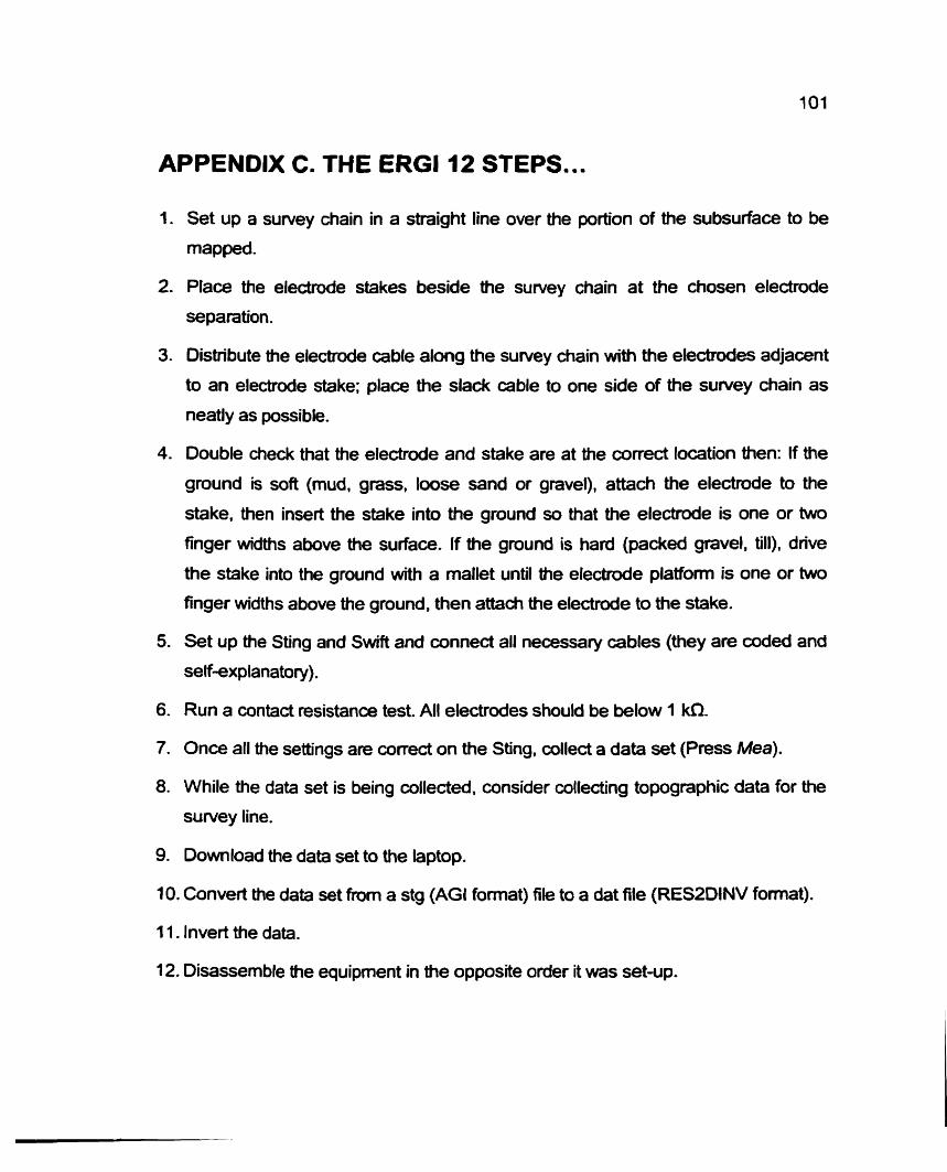
APPENDIX C. THE ERG1 12 STEPS ... 1. Set up a survey chain in a straight line over the portion of the subsurface to be
mapped.
2. Place the eledrode stakes beside the survey chain at the chosen electrode
separation.
3. Distribute the electrode cable along Me survey chain with the electrodes adjacent
to an electrode stake; place the slack cable to one side of the survey chain as
neatly as possible.
4. Double check that the electrode and stake are at the correct location then: If the
ground is soft (mud, grass, loose sand or gravel), attach the electrode to the
stake, then insert the stake into the ground so that the electrode is one or two
finger widths above the surface. If the ground is hard (packed gavel, till), drive
the stake into the ground with a mallet until the electrode platform is one or two
finger widths above the ground, then attach the electrode to the stake.
5. Set up the Sting and Swift and connect all necessary cables (they are coded and
self-explanatory).
6. Run a contact resistance test. All electrodes should be below 1 WI.
7. Once all the settings are correct on the Sting, cdlect a data set (Press Ma).
8. While the data set is being collected, consider collecting topographic data for the
survey line.
9. Download the data set to the laptop.
10. Convert the data set from a stg (AGI format) file to a dat file (RES2DINV fonnat).
1 1. Invert the data.
12. Disassemble the equipment in the opposite order it was set-up.

APPENDIX D. COORDlNATES FOR ALL OF THE DATA
PRESENTED IN THE BODY OF THE THESIS
The coordinates for the ERG1 surveys and for the vibracores were
collected with a hand held GPS receiver. No corrections have been applied to the
coordinates. Locations from the upper Columbia River, B.C., are described using
Universal Transverse Mercator (UTM) coordinates relative to the WGS84 datum.
Locations from the Rhine-Meuse Delta, the Netherlands are described using
Dutch national grid system (NLRD - Rijksdriehoeksrneting Nederland)
coordinates relative to the Besse11842 datum.
Start End Easting Northing Easting Northing
ERG1 Surveys BTC102 532171 5651760 532131 5651722 BTC103 532171 5651760 532131 5651722 BTC30 1 532230 5651817 532625 5652198 BLM101 532257 5651773 532403 5651893 BTS20 1 532365 5651566 532443 5651634 BTS40 1 532354 5651696 532442 5651586 HMS101 533527 5650415 533599 5650494 HMS201 533503 5650466 533586 5650398 Vi bracores BTS2-74 532421 5651615 HMS1-23.3 533543 5650432
Table 1 UTM Coordinates for data from the upper Columbia River, 8. C.

Start End Easting Northing Easting Northinq
ERG1 Surveys CSlOl CS102 CS103 cs104 CS105 CS106 CS107 CS108 NL9309101 NL9309103
Table 2 NLRD coordinates for data from the Rhine-Meuse Delta, the Netherlands.
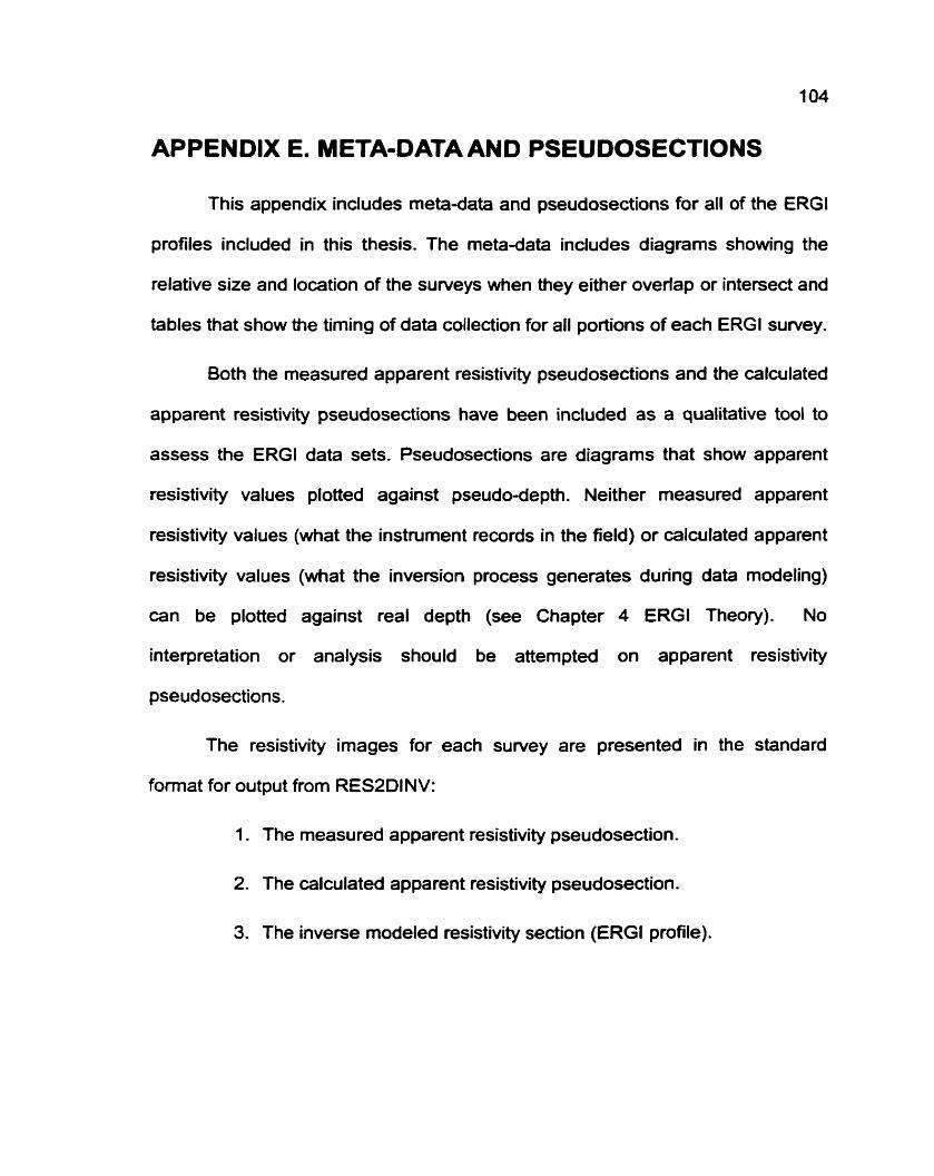
APPENDIX E. META-DATA AND PSEUDOSECTIONS
This appendix includes meta-data and pseudosections for all of the ERG1
profiles included in this thesis. The meta-data includes diagrams showing the
relative size and location of the surveys when they either overlap or intersect and
tables that show the timing of data collection for all portions of each ERG1 survey.
Both the measured apparent resistivity pseudosections and the calculated
apparent resistivity pseudosections have been included as a qualitative tool to
assess the ERG1 data sets. Pseudosections are diagrams that show apparent
resistivity values plotted against pseudo-depth. Neither measured apparent
resistivity values (what the instrument records in the field) or calculated apparent
resistivity values (what the inversion process generates during data modeling)
can be plotted against real depth (see Chapter 4 ERG1 Theory). No
interpretation or analysis should be attempted on apparent resistivity
pseudosections.
The resistivity images for each survey are presented in the standard
format for output from RES2DINV:
1. The measured apparent resistivity pseudosection.
2. The calculated apparent resistivity pseudosection.
3. The inverse modeled resistivity section (ERGI profile).

E. 1 Data from the Upper Columbia River, British Columbia
Figure 28 Oblique aerial photograph showing the relative location of the ERG1 study sites on the upper Columbia River in British Columbia. The reach of river shown in the photo is approximately 2.5 km long.
Table 3 Location, survey series, survey number, survey goal, and cross- reference thesis section number for data from the upper Columbia River, B. C.
See Thesis Section
7.2
7.1
6.1
6.2
6.2
Location
Beavertail Channel-Fill
Y
Y
Beavertail Crevasse-Splay
Herron Meadow Crevasse-Splay
Survey Series
BTC1
BTC3
ELM1
BTS2 BTS4
HMSl HMS2
Survey Number
BTC101 BTC103
BTC301
BMLtOl
BTSZOl BTS401
HMSIO1 HMS201
Survey Goal
Comparing Arrays
Combining Land and Water
Imaging Channel-Fills
Imaging Crevassesplays
Imaging Crevasse-Splays
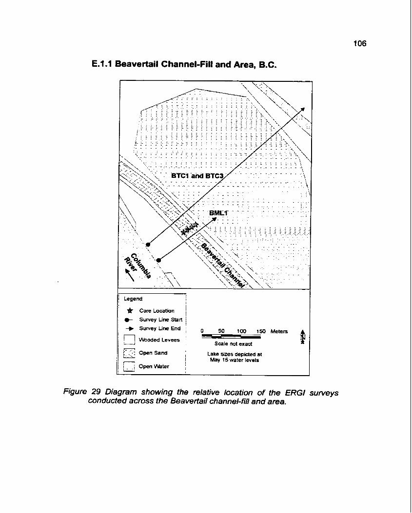
E.l .I Beavertail Channel-Fill and Area, B.C.
. . . . . . . . . - - - - - -
. .
1 Legend i I / f Core Location ,
j t s u m y tine Start 1 I
i -) Survey line End ; 0 50 1 0 0 150 Meters
Wooded Levees I -
Scale not exact
Open Sand 1: a I I Lake sizes depicted at
F - May 1 5 water levels 1 ; ; Open Water -
Figure 29 Diagram showing the relative location of the ERG1 surveys conducted across the Beavertail channel-fill and area.
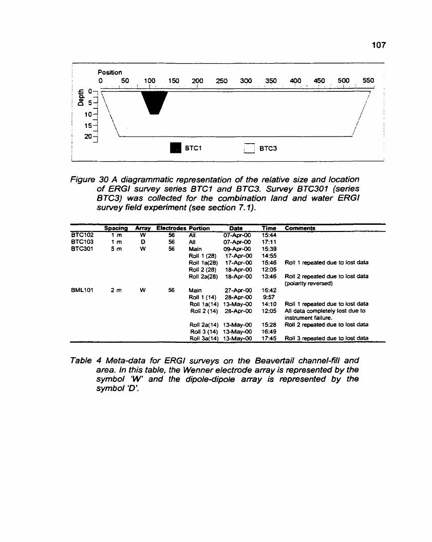
I Position ! 0 I ; , . I
0 150 200 250 300 350 400 450 590 , 550 ' , I ' ) I , : , I f , ' . , . '
! c 07- i = i
i :
a 5 4 ;
/ I
\ ,/' ! 201
Figure 30 A diagrammatic representation of the relative size and location of ERGI survey series BTCI and BTC3. Survey BTC301 (series BTC3) was collected for the combination land and water ERGI survey field experiment (see section 7.1).
Spacing Array Electrodes Portion Date Time Comments BTC102 1 m W 56 All Of-Apr-00 15:44 BTC103 1 m D 56 All 07-Apr-00 17:11 BTC301 5 rn W 56 Main 09-Apr-00 1539
Roll 1 (28) 17-Apr-00 1455 Roll la(28) 17-Apr-00 15:46 Roll 1 repeated due to lost data Roll 2 (28) 1&Apr-00 12:05 Roll 2a(28) 18-Apr-00 13:46 Roll 2 repeated due to lost data
(polarity reversed) BML101 2 m W 56 Main 27-Apr-00 16:42
Roil 1 (14) 28-Apr-00 957 Roll la(l4) 13-May- 14:10 Roll 1 repeated due to lost data Roli 2 (14) 28-Apr-OO 12:05 All data completely Iost due to
instrument failure. Roll 2a(14) 13-May4 1528 Roll 2 repeated due to Iost data Rolf 3 (14) 13-May-00 16:49 Roll 3a(14) 13-May-00 1 7:45 Roll 3 repeated due to lost data
Table 4 Meta-data for ERG1 surveys on the Beavertail channel-fill and area. h this table, the Wenner electrode array is represented by the symbol 'W' and the dipole-dipole array is represented by the symbol 'D:

Figure 3 1 ERGl Survey B TC 102.
Figure 32 ERGl Survey BTCIOJ.
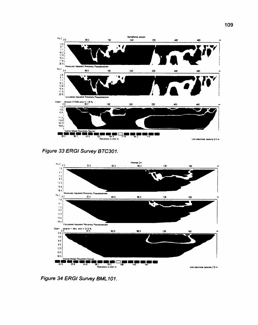
Figure 33 ERGl Survey BTC301.
Reunmtv ~n onm rn
Figure 34 ERGl Survey BML 101.
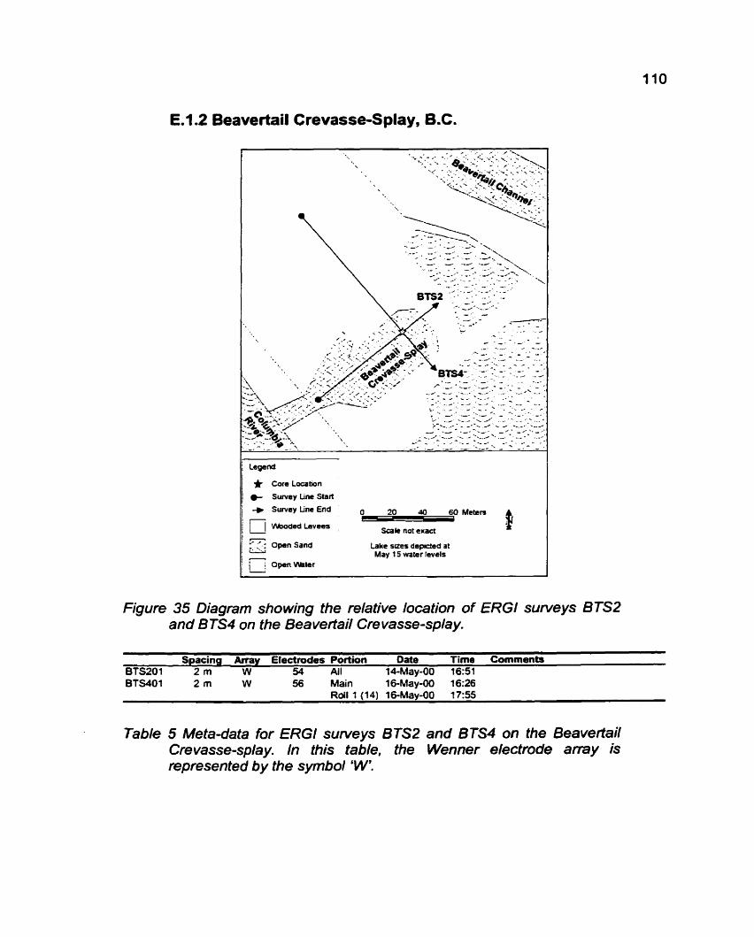
E.1.2 Beavertail Crevasse-Splay, B.C.
_-. ._... - ..-- -._ - -, - _ . I _ a ..- ./;. .., - ..- - ... . -_ * - _ J '-. _ -. I . > '
* Care Location
t Survey tine Start
j 4 Survey line End 20 a C
Scale not u a c t 1 - I I Open Sand Lake sues depcted at
May 15 wafer levels
1 open mter
Figure 35 Diagram showing the relative location of ERGl surveys BTS2 and BTS4 on the Beaverfail Crevasse-splay.
Spacing Array Electrodes Portion Date Time Comments BTS201 2 m W 54 All 14-May-00 16:51 BTS401 2 m W 56 Main 16-~a&UO 16:26
Rdl 1 (14) 16-May40 1755
Table 5 Meta-data for ERGl surveys BTSZ and BTS4 on the Beavertail Crevasse-splay. In this table, the Wenner electrode array is represented by the symbol 'W'.
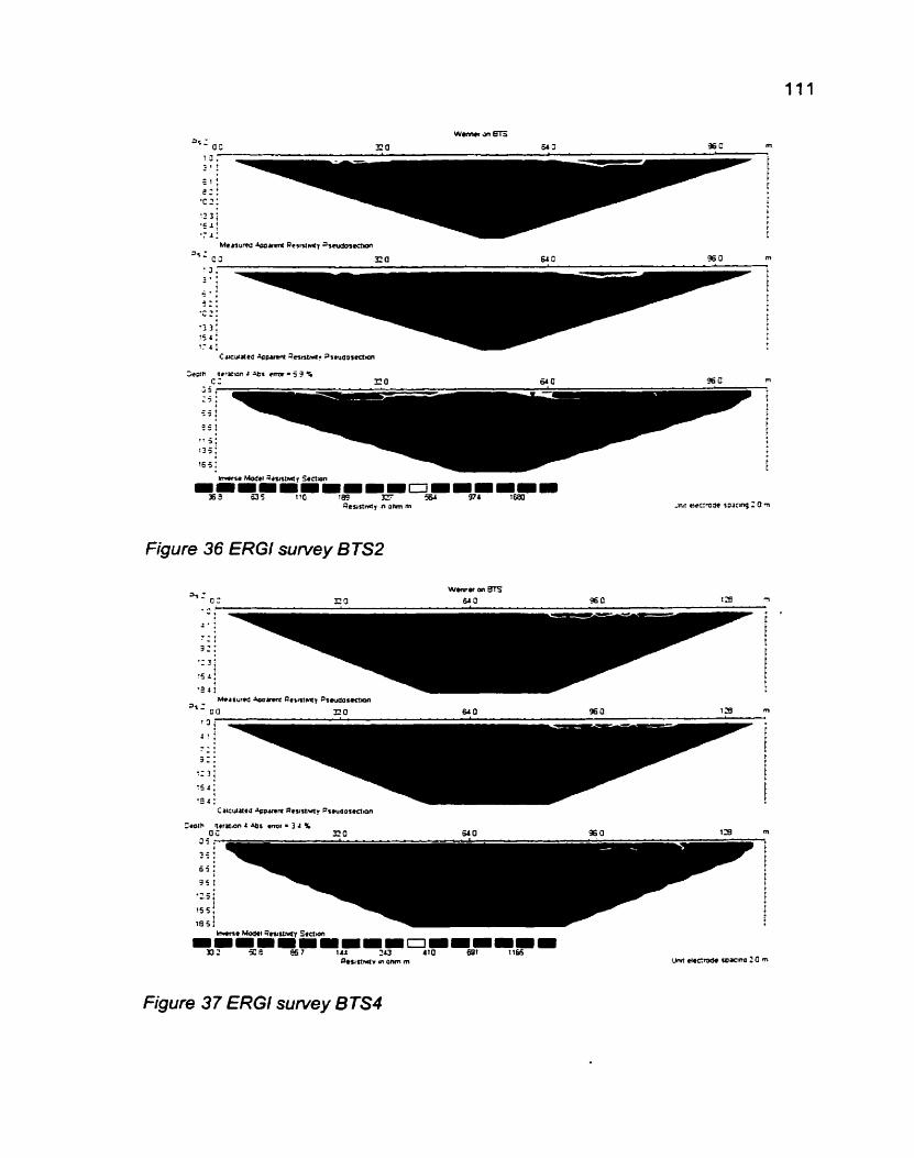
Figure 36 ERGI survey B TS2
ire m
hum* Model ilrurtnpy Sealon
a, 141 u Reunmv m onm rn
Figure 37 ERG1 survey BTS4
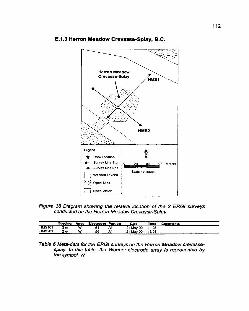
E.1.3 Herron Meadow Crevasse-Splay, B.C.
Herron Meadow Crevasse-Splay
-.-A --.---/-.... "\,
\ - ._._ - - _ _ _ ' --__/ . .. :. I- .-.
' - - - .--'. - / - ; '\..
Legend
* Core Location ' P + Survey tine Start I 20 60 -+ Survey tine End : -
Scale not exact wooded Levees
I
3 Open Sand u
Open Water d
Figure 38 Diagram showing the relative location of the 2 ERGl surveys conducted on the Henon Meadow Crevasse-Splay.
Spacing Array Electrodes Portion Date Time Comments HMSfOl 2 m W 51 AII 21 -Mav-M) 1 1 :Of3
Table 6 Meta-data for the ERGl surveys on the Herron Meadow crevasse- splay. In this table, the Wenner electrode array is represented by the symbol 'W'
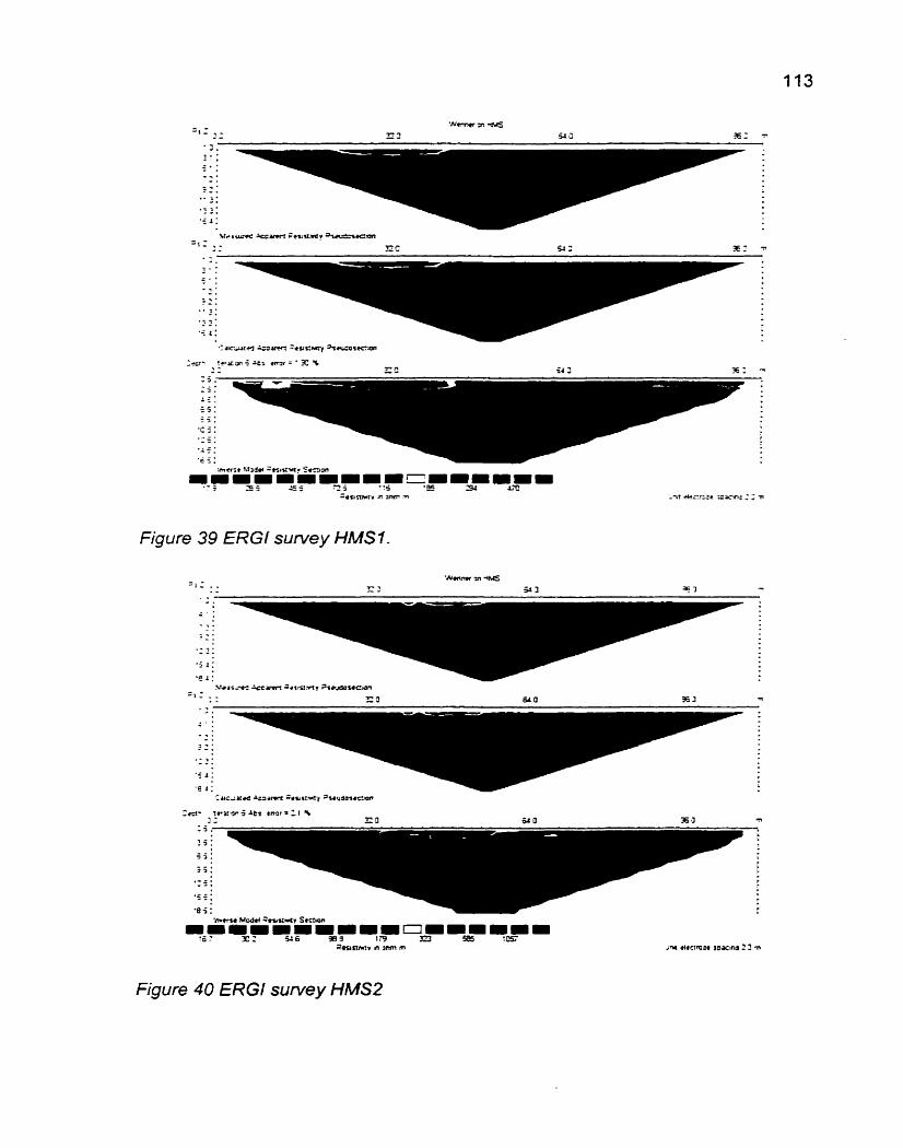
Figure 39 ERGI survey HMS1.
Figure 40 ERG1 survey HMS2
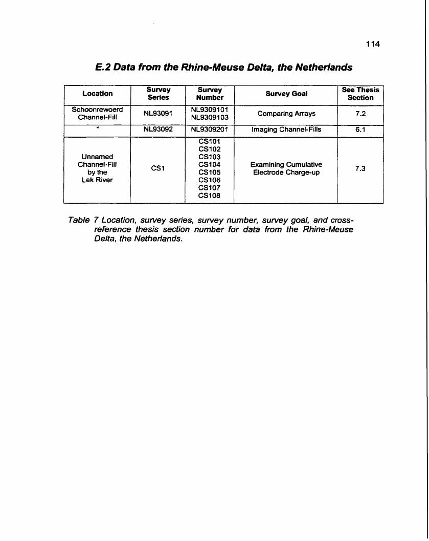
E.2 Data from the Rhine-Meuse Delta, the Netherlands
Table 7 Location, suwey series, suwey number, survey goal, and cross- reference thesis section number for data from the Rhine-Meuse Delta, the Netherlands.
Location
Schoonrewoerd Channel-Fill
Y
Unnamed Channel-Fill
by the Lek River
Survey Series
NL9309'
NL93092
CS1
Survey Number
NL9309101 NL9309103
NL9309201
CS101 CS102 CS103 CS104 CSIOS CS106 CS107 CS108
Survey Goal
Comparing Arrays
Imaging Channel-Fills
Examining Cumulative Electrode Charge-up
See Thesis Section
7.2
6.1
7-3
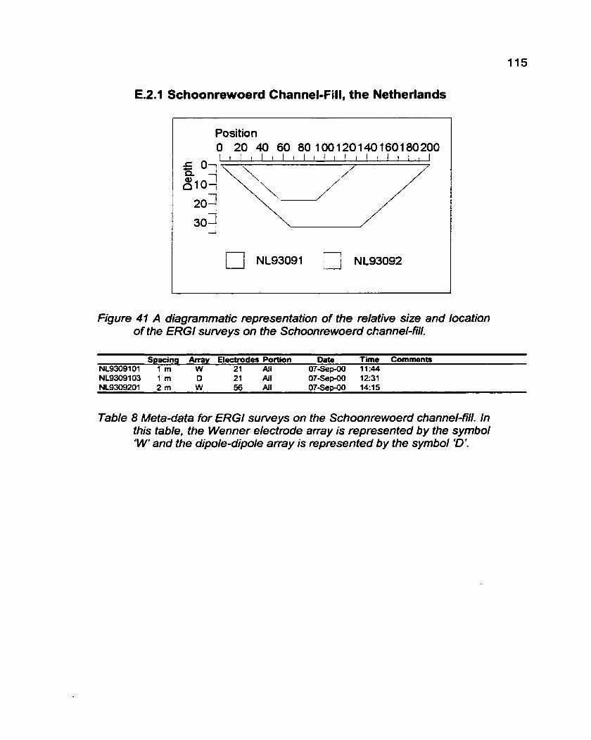
E.2.1 Schoonrewoerd Channel-Fill, the Netherlands --
Position 0 20 40 60 80 100120140160180200
[ I t ! l l r l l l ! ! ~ l ~ l l ~ l ~
20:
304 i
NL93091 NL93092
1
Figure 41 A diagrammatic representation of the relative size and location of the ERG1 surveys on the Schoonrewoerd channel-fil.
Spacing Array Electrodes Portion Date Time Comments NU309101 1 rn W 21 All 07-Sep-00 11:44 NL9309103 1 m D 21 All 07-~e&0 12:31 NU309201 2 rn W 56 All 07-Sep00 14: 1 5
Table 8 Meta-data for ERG1 surveys on the Schoonrewoerd channel-fill. In this table, the Wenner electrode array is represented by the symbol 'W' and the dipole-dipole array is represented by the symbol '0'.
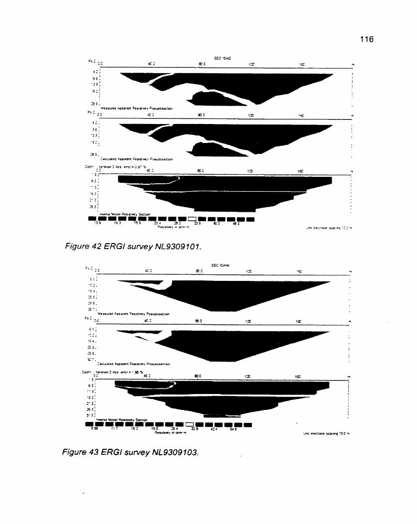
Figure 42 ERG1 survey NL9309 70 7.
'Jna rcc.tccc W w n q 'GO n
Figure 43 ERG1 survey NL9309 703.

Figure 44 ERGl sunley NL9309207.
E.2.2 Unnamed Channel-Fills by the Lek River, the Netherlands
Spacinq Array Electrodes Ponion Date Time Comments CSlS! 10 m W 23 All 21-Sep-00 1 l:16 CS 102 10 m S 28 All 27-Sep-UO 11:36 CS703 1 O rr, W 28 All 27-SegOO ;2:24 CS 10.: 10 rn S 23 All 21-Sew0 12:47 CS 105 10 m Cnl 29 All 21-Sep-00 ?3:11 CS ! 06 :O rn S 28 All 21-Sep-00 1332 CS 107 10 m W 23 All 21-S~p-00 13~59 Cll C8 1 C n S 28 All 21-Sep-00 14:52
Table 9 Meta-data for ERGl surveys at the study site adjacent to the Lek River. In this table, the Wenner electrode aray is represented by the symbol 'W' and the Wenner-Schlumberger array is represented by the symbol 'S'.
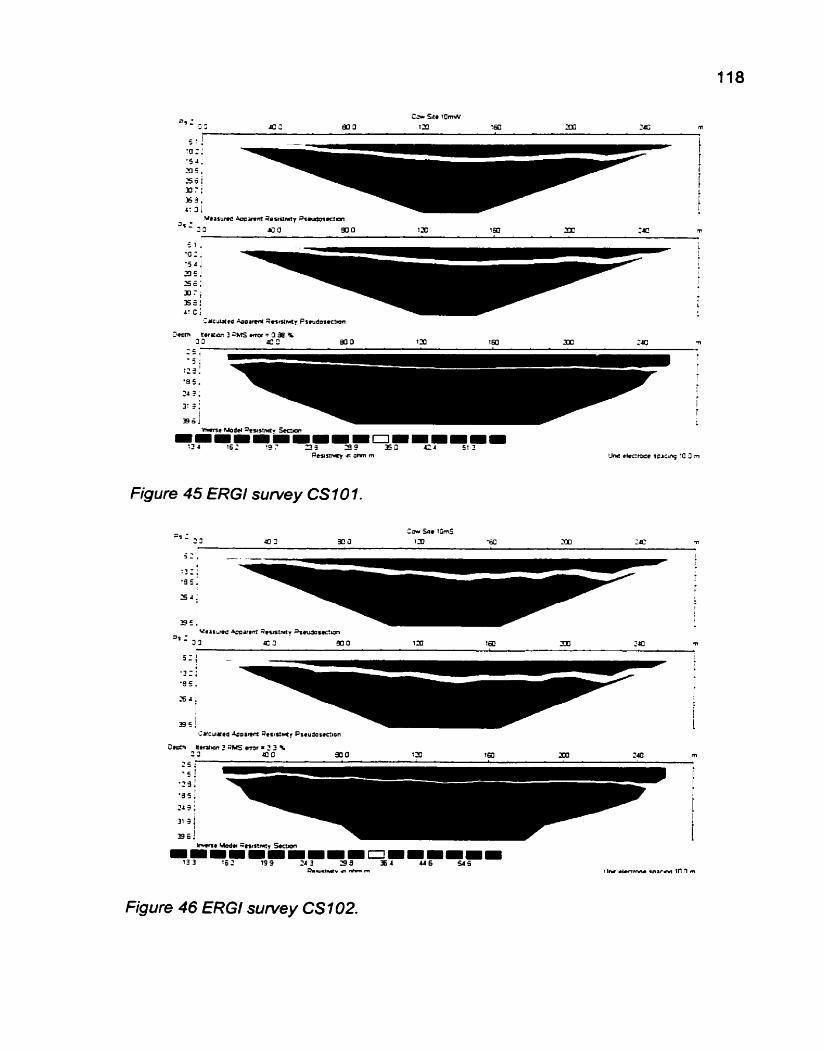
Figure 45 ERGl sunley CS 10 1.
Figure 46 ERGl survey CS 102.

Figure 47 ERG1 survey CS 103.
Figure 48 ERG1 survey CS 7 04.

Figure 49 ERGl survey CS705.
' m e M o d u 4 . u s t m t y Sutun
s st sf my as^-^--^^ 9 2 . - =.u.~WV rm nrrn m
Figure 50 ERGl survey CS 106.
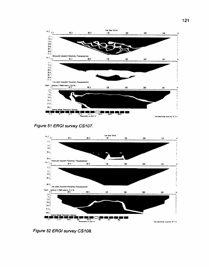
'Jw -mar so&c:nq
Figure 5 1 ERG1 survey CS 10 7.
>*urn trrtrton 3 ah6 mor = 31 3 % C - roo 300 . -
Sru.rlrrr n m m
Figure 52 ERG1 survey CS 108.