Embed Size (px)
Citation preview

SAND REPORT
SAND2002-3834 Unlimited Release Printed November 2002 Electrical-Impedance Tomography for Opaque Multiphase Flows in Metallic (Electrically-Conducting) Vessels
Scott Gayton Liter, John R. Torczynski, Kim A. Shollenberger and Steven L. Ceccio
Prepared by Sandia National Laboratories Albuquerque, New Mexico 87185 and Livermore, California 94550 Sandia is a multiprogram laboratory operated by Sandia Corporation, a Lockheed Martin Company, for the United States Department of Energy’s National Nuclear Security Administration under Contract DE-AC04-94-AL85000. Approved for public release; further dissemination unlimited.

Issued by Sandia National Laboratories, operated for the United States Department of Energy by Sandia Corporation.
NOTICE: This report was prepared as an account of work sponsored by an agency of the United States Government. Neither the United States Government, nor any agency thereof, nor any of their employees, nor any of their contractors, subcontractors, or their employees, make any warranty, express or implied, or assume any legal liability or responsibility for the accuracy, completeness, or usefulness of any information, apparatus, product, or process disclosed, or represent that its use would not infringe privately owned rights. Reference herein to any specific commercial product, process, or service by trade name, trademark, manufacturer, or otherwise, does not necessarily constitute or imply its endorsement, recommendation, or favoring by the United States Government, any agency thereof, or any of their contractors or subcontractors. The views and opinions expressed herein do not necessarily state or reflect those of the United States Government, any agency thereof, or any of their contractors. Printed in the United States of America. This report has been reproduced directly from the best available copy. Available to DOE and DOE contractors from
U.S. Department of Energy Office of Scientific and Technical Information P.O. Box 62 Oak Ridge, TN 37831 Telephone: (865)576-8401 Facsimile: (865)576-5728 E-Mail: [email protected] Online ordering: http://www.doe.gov/bridge
Available to the public from
U.S. Department of Commerce National Technical Information Service 5285 Port Royal Rd Springfield, VA 22161 Telephone: (800)553-6847 Facsimile: (703)605-6900 E-Mail: [email protected] Online order: http://www.ntis.gov/help/ordermethods.asp?loc=7-4-0#online
2

SAND2002-3834 Unlimited Release
Printed November 2002
Electrical-Impedance Tomography for Opaque Multiphase Flows
in Metallic (Electrically-Conducting) Vessels
Scott Gayton Liter and John R. Torczynski Engineering Sciences Center Sandia National Laboratories
P.O. Box 5800 Albuquerque, New Mexico 87185-0834
Kim A. Shollenberger
Mechanical Engineering Department California Polytechnic State University
San Luis Obispo, CA 93407
Steven L. Ceccio Department of Mechanical Engineering and Applied Mechanics
University of Michigan Ann Arbor, Michigan 48109-2125
Abstract A novel electrical-impedance tomography (EIT) diagnostic system, including hardware and software, has been developed and used to quantitatively measure material distributions in multiphase flows within electrically-conducting (i.e., industrially relevant or metal) vessels. The EIT system consists of energizing and measuring electronics and seven ring electrodes, which are equally spaced on a thin nonconducting rod that is inserted into the vessel. The vessel wall is grounded and serves as the ground electrode. Voltage-distribution measurements are used to numerically reconstruct the time-averaged impedance distribution within the vessel, from which the material distributions are inferred. Initial proof-of-concept and calibration was completed using a stationary solid-liquid mixture in a steel bench-top standpipe. The EIT system was then deployed in Sandia's pilot-scale slurry bubble-column reactor (SBCR) to measure material distributions of gas-liquid two-phase flows over a range of column pressures and superficial gas flow rates. These two-phase quantitative measurements were validated against an established
3

gamma-densitometry tomography (GDT) diagnostic system, demonstrating agreement to within 0.05 volume fraction for most cases, with a maximum difference of 0.15 volume fraction. Next, the EIT system was combined with the GDT system to measure material distributions of gas-liquid-solid three-phase flows in Sandia's SBCR for two different solids loadings. Accuracy for the three-phase flow measurements is estimated to be within 0.15 volume fraction. The stability of the energizing electronics, the effect of the rod on the surrounding flow field, and the unsteadiness of the liquid temperature all degrade measurement accuracy and need to be explored further. This work demonstrates that EIT may be used to perform quantitative measurements of material distributions in multiphase flows in metal vessels.
Acknowledgements This project was funded under the Laboratory Directed Research and Development (LDRD) program and Sandia National Laboratories. The authors gratefully acknowledge the interactions with the following individuals. Dr. Bernard A. Toseland and Dr. Bharatt L. Bhatt of Air Products and Chemicals, Inc., provided useful guidance and information on the use and characterization of industrial-scale bubble columns. Dr. Douglas R. Adkins, Dr. Nancy B. Jackson, and Dr. Timothy J. O’Hern of Sandia National Laboratories helped establish Sandia’s SBCR facility and helped in the development of the GDT system. Dr. Ann Tassin-Leger and Dr. Darin L. George, both formerly of the University of Michigan, and Paul R. Tortora of the University of Michigan collaborated closely on the development and application of the EIT system. Dr. Daniel A. Lucero provided laboratory space and various supplies for completion of the benchtop proof-of-concept experiments. The authors give particular thanks to the excellent technical support of the following individuals, both currently and formerly of Sandia National Laboratories: Raymond O. Cote, Thomas W. Grasser, Mr. John Oelfke, Jaime N. Castañeda, Rocky J. Erven, John J. O’Hare, the late C. Buddy Lafferty, and W. Craig Ginn. Raymond O. Cote is especially thanked for the excellent skill and care he used to fabricate the EIT electrode rod. Dr. Michael R. Prairie and Dr. Arthur C. Ratzel of Sandia National Laboratories are both thanked for their excellent management and continuing support of this work.
4

Contents Figures..............................................................................................................................................6 Tables...............................................................................................................................................8 Nomenclature...................................................................................................................................8 1. Background and Introduction..................................................................................................11
1.1. Overview and Motivation ..............................................................................................11 1.2. Measurement Techniques ..............................................................................................12 1.3. Summary of Previous Work...........................................................................................14
2. Theory .....................................................................................................................................14 2.1. Electrical-Impedance Tomography (EIT)......................................................................14 2.2. Gamma-Densitometry Tomography (GDT) ..................................................................19 2.3. Combined EIT and GDT for Three-Phase Measurements.............................................21
3. Diagnostic Systems .................................................................................................................24 3.1. EIT Apparatus................................................................................................................24 3.2. GDT Apparatus..............................................................................................................26
4. Experiments.............................................................................................................................27 4.1. Benchtop Validation Test ..............................................................................................27 4.2. Sandia’s Slurry Bubble-Column Reactor (SBCR) Facility ...........................................29 4.3. Experimental Procedure for Measurements in Sandia’s SBCR.....................................32 4.4. Experimental Material Properties ..................................................................................34 4.5. Sources of Uncertainty...................................................................................................35
5. Experimental Results and Discussion .....................................................................................36 5.1. Benchtop Validation Measurements ..............................................................................36 5.2. Two-Phase Measurements .............................................................................................37 5.3. Three-Phase Measurements ...........................................................................................45
6. Conclusions and Future Recommendations ............................................................................52 References......................................................................................................................................53 Appendix........................................................................................................................................56
5

Figures Figure 1. Schematic of an EIT system applied to an electrically insulating (nonconducting)
vessel.......................................................................................................................... 16 Figure 2. Schematic of an EIT system applied to an electrically conducting vessel. ............... 17 Figure 3. Photograph of verification experiment showing the EIT electronics, the electrode rod
with seven copper ring electrodes (the top eighth ring shown is a plastic seal), and the standpipe. ............................................................................................................. 25
Figure 4. Photographs of the circuits boards inside the EIT electronics box............................ 26 Figure 5. A schematic of the GDT system in the horizontal plane. .......................................... 27 Figure 6. Schematic of verification experiment consisting of an electrode rod inserted
coaxially in an electrically conducting standpipe filled with nonconducting solid polystyrene particles and liquid. ................................................................................ 28
Figure 7. Photograph of the Sandia slurry bubble-column reactor facility. Also shown is the vault for the gamma source mounted on the two-axis automated traverse................ 29
Figure 8. Photograph of a cross sparger similar to that used in this study to inject air into the bottom of the bubble column..................................................................................... 30
Figure 9. Schematic of EIT system applied to Sandia’s slurry bubble-column reactor (SBCR). Shown on the right is a photograph of the SBCR (0.48-m ID). The bottom left shows predictions of voltage contours in a cross-section of the SBCR for two cases, one of constant conductivity in the top half, and one of variable conductivity in the bottom half................................................................................................................. 31
Figure 10. (a) Computational mesh corresponding to one-quarter of the interior of the SBCR with the EIT rod inserted along a diameter. (b) Voltage contours computed for a uniform electrical conductivity throughout the domain with current injection from electrode 4.................................................................................................................. 33
Figure 11. Plot of the EIT reconstructed particle-bed height versus the measured particle-bed height in the steel standpipe....................................................................................... 36
Figure 12. Comparison of symmetric radial gas volume fraction profiles from EIT and GDT for a column pressure =colp 103 kPa and a superficial gas velocity 10 cm/s. ..... 39 =gu
Figure 13. Comparison of symmetric radial gas volume fraction profiles from EIT and GDT for a column pressure =colp 103 kPa and a superficial gas velocity 15 cm/s. ..... 39 =gu
Figure 14. Comparison of symmetric radial gas volume fraction profiles from EIT and GDT for a column pressure =colp 103 kPa and a superficial gas velocity 20 cm/s. ..... 40 =gu
Figure 15. Comparison of symmetric radial gas volume fraction profiles from EIT and GDT for a column pressure =colp 103 kPa and a superficial gas velocity 25 cm/s. ..... 40 =gu
Figure 16. Comparison of symmetric radial gas volume fraction profiles from EIT and GDT for a column pressure =colp 207 kPa and a superficial gas velocity 10 cm/s. ..... 41 =gu
Figure 17. Comparison of symmetric radial gas volume fraction profiles from EIT and GDT for a column pressure =colp 207 kPa and a superficial gas velocity 15 cm/s. ..... 41 =gu
Figure 18. Comparison of symmetric radial gas volume fraction profiles from EIT and GDT for a column pressure =colp 207 kPa and a superficial gas velocity 20 cm/s. ..... 42 =gu
6

Figure 19. Comparison of symmetric radial gas volume fraction profiles from EIT and GDT for a column pressure =colp 207 kPa and a superficial gas velocity 25 cm/s. ..... 42 =gu
Figure 20. Comparison of symmetric radial gas volume fraction profiles from EIT and GDT for a column pressure =colp 310 kPa and a superficial gas velocity 10 cm/s. ..... 43 =gu
Figure 21. Comparison of symmetric radial gas volume fraction profiles from EIT and GDT for a column pressure =colp 310 kPa and a superficial gas velocity 15 cm/s. ..... 43 =gu
Figure 22. Comparison of symmetric radial gas volume fraction profiles from EIT and GDT for a column pressure =colp 310 kPa and a superficial gas velocity 20 cm/s. ..... 44 =gu
Figure 23. Plot of the bulk-averaged gas fraction as a function of superficial gas velocity and column pressure, from GDT measurements. ............................................................. 44
Figure 24. Plot of the bulk-averaged gas fraction as a function of superficial gas velocity and column pressure, from EIT measurements. ............................................................... 45
Figure 25. Radial material phase-volume-fraction profiles for a nominal slurry concentration =nom
sε 0%, with a column pressure =colp 103 kPa and a superficial gas velocity 10 cm/s.............................................................................................................. 47 =gu
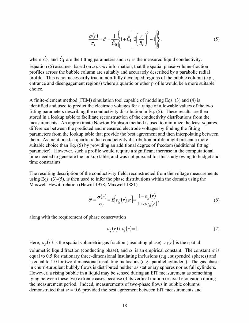
Figure 26. Radial material phase-volume-fraction profiles for a nominal slurry concentration =nom
sε 0%, with a column pressure =colp 207 kPa and a superficial gas velocity 10 cm/s.............................................................................................................. 48 =gu
Figure 27. Radial material phase-volume-fraction profiles for a nominal slurry concentration =nom
sε 4%, with a column pressure =colp 103 kPa and a superficial gas velocity 10 cm/s.............................................................................................................. 48 =gu
Figure 28. Radial material phase-volume-fraction profiles for a nominal slurry concentration =nom
sε 4%, with a column pressure =colp 207 kPa and a superficial gas velocity 10 cm/s.............................................................................................................. 49 =gu
Figure 29. Radial material phase-volume-fraction profiles for a nominal slurry concentration =nom
sε 8%, with a column pressure =colp 103 kPa and a superficial gas velocity 10 cm/s.............................................................................................................. 49 =gu
Figure 30. Radial material phase-volume-fraction profiles for a nominal slurry concentration =nom
sε 8%, with a column pressure =colp 207 kPa and a superficial gas velocity 10 cm/s.............................................................................................................. 50 =gu
Figure 31. Radial material phase-volume-fraction profiles for a nominal slurry concentration =nom
sε 4%, with a column pressure =colp 103 kPa and a superficial gas velocity 10 cm/s, and calculated with a conductivity ratio =gu lr σσσ )(41.1~ = . .............. 50
Figure 32. Radial material phase-volume-fraction profiles for a nominal slurry concentration =nom
sε 4%, with a column pressure =colp 207 kPa and a superficial gas velocity 10 cm/s, and calculated with a conductivity ratio =gu lr σσσ )(41.1~ = . .............. 51
7

Figure 33. Radial material phase-volume-fraction profiles for a nominal slurry concentration =nom
sε 8%, with a column pressure =colp 103 kPa and a superficial gas velocity 10 cm/s, and calculated with a conductivity ratio =gu lr σσσ )(94.0~ = . ............. 51
Figure 34. Radial material phase-volume-fraction profiles for a nominal slurry concentration =nom
sε 8%, with a column pressure =colp 207 kPa and a superficial gas velocity 10 cm/s, and calculated with a conductivity ratio =gu lr σσσ )(94.0~ = . ............. 52
Tables Table 1. Various industrial applications that would benefit from improved capability to
measure spatial volumetric phase fractions. .............................................................. 12 Table 2. Some noninvasive diagnostic techniques reported in the literature used to measure
spatial volumetric phase fractions. ............................................................................ 13 Table 3. Operating conditions for the two- and three-phase tests in the SBCR. ..................... 32 Table 4. Properties of the phase materials used for the material distribution reconstructions. 35 Table 5. Measured and predicted particle-bed heights for 6 different tests, 3 with copper
electrodes and 3 with stainless steel electrodes. ........................................................ 37 Table 6. Comparison of EIT and averaged GDT measurements of gas volume fractions for the
11 different two-phase operating conditions listed in Table 4. ................................. 38 Table 7. Predicted bulk-averaged phase volume fractions for the 6 three-phase cases
measured and listed in Table 4. ................................................................................. 46 Table 8. Predicted bulk-averaged volumetric phase-fractions for the cases of 4% and 8%
nominal solids loading, using a scaled conductivity ratio. ........................................ 47
Nomenclature Roman Symbols
10 ˆ,ˆ aa coefficients for GDT normalized parabolic radial attenuation profile
10ˆ,ˆ bb coefficients for GDT normalized parabolic line-averaged attenuation profile
0c speed of light in vacuum, m/s 8103×
10 ˆ,ˆ CC parabolic fitting parameters for EIT parabolic radial conductivity profile
σC conductivity-ratio scaling factor
d steel standpipe inner diameter, m
pd nonconducting particle diameter, m
[ ]E Maxwell-Hewitt correlation relating nonconducting phase fraction to σ~
8

f excitation frequency of AC current for EIT measurement, Hz
( )rfµ time-averaged, normalized radial attenuation coefficient
bh particle-bed height in steel standpipe, m
lh liquid-fill height in steel standpipe, m
colp headspace pressure in bubble column, kPa
r radial position variable, m
iR internal radius of SBCR, 0.24 m
gu superficial gas velocity, cm/s
0I intensity (counts per second) of gamma beam at source aperture
( )xI intensity (counts per second) of gamma beam at detector
gI for an empty (gas-filled) column ( )xI
lI for a full (liquid-filled, stationary) column ( )xI
j flux of electric charge at domain boundary for EIT measurement, A/m 2
( )xL chord length of gamma beam passing through multiphase flow domain at position x , m
n unit normal vector
N number of electrodes in EIT system
V voltage for EIT measurement, V
x horizontal position of GDT while scanning across bubble column diameter at height , m y
( )xX i cumulative length in gamma beam path ( )xL of material phase i (gas, liquid, solid) at position
slg ,,=x , m
y vertical position (height) of GDT for a single horizontal scan across the bubble column diameter, m
Greek Symbols α empirical constant used in Maxwell-Hewitt relation
0ε permittivity of vacuum, 8 12108542. −× F/m
ε~ dielectric constant, 1~ ≥ε
( )xiε cumulative volume fraction of phase slgi ,,= (gas, liquid, solid) along length ( )xL
9

( )riε radial volume fraction of phase slgi ,,= (gas, liquid, solid) nomsε nominal solids-loading volume fraction
iµ attenuation coefficient of material gi sl,,= (gas, liquid, solid)
( )xµ ray-averaged attenuation coefficient along length ( )xL
( )rµ radial attenuation coefficient
σ bulk electrical conductivity, µS/cm or S/m
( )rσ radial electrical conductivity distribution, µS/cm
σ~ normalized radial electrical conductivity distribution, ( ) lr σσ
lls,~σ normalized radial electrical conductivity distribution of liquid-solid mixture
compared to full liquid, ( ) lls r σσ
lsgls,~σ normalized radial electrical conductivity distribution of three-phase mixture
compared to fully liquid-solid mixture, ( ) ( )rr lsσσ
lσ electrical conductivity of the liquid phase, µS/cm
( )xΨ normalized line-averaged attenuation coefficient along length ( )xL Acronyms EIT electrical-impedance tomography
EPROM erasable programmable read-only memory chip
FEM finite-element method
GDT gamma-densitometry tomography
SBCR slurry bubble-column reactor
10
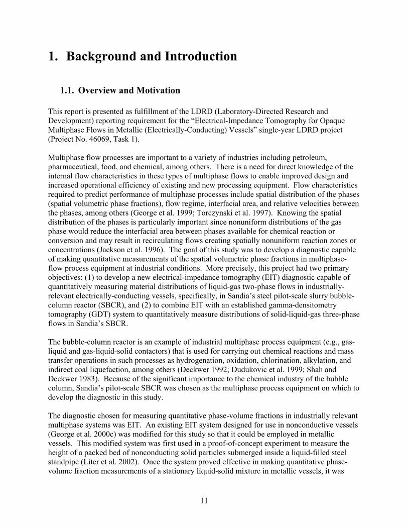
1. Background and Introduction
1.1. Overview and Motivation This report is presented as fulfillment of the LDRD (Laboratory-Directed Research and Development) reporting requirement for the “Electrical-Impedance Tomography for Opaque Multiphase Flows in Metallic (Electrically-Conducting) Vessels” single-year LDRD project (Project No. 46069, Task 1). Multiphase flow processes are important to a variety of industries including petroleum, pharmaceutical, food, and chemical, among others. There is a need for direct knowledge of the internal flow characteristics in these types of multiphase flows to enable improved design and increased operational efficiency of existing and new processing equipment. Flow characteristics required to predict performance of multiphase processes include spatial distribution of the phases (spatial volumetric phase fractions), flow regime, interfacial area, and relative velocities between the phases, among others (George et al. 1999; Torczynski et al. 1997). Knowing the spatial distribution of the phases is particularly important since nonuniform distributions of the gas phase would reduce the interfacial area between phases available for chemical reaction or conversion and may result in recirculating flows creating spatially nonuniform reaction zones or concentrations (Jackson et al. 1996). The goal of this study was to develop a diagnostic capable of making quantitative measurements of the spatial volumetric phase fractions in multiphase-flow process equipment at industrial conditions. More precisely, this project had two primary objectives: (1) to develop a new electrical-impedance tomography (EIT) diagnostic capable of quantitatively measuring material distributions of liquid-gas two-phase flows in industrially-relevant electrically-conducting vessels, specifically, in Sandia’s steel pilot-scale slurry bubble-column reactor (SBCR), and (2) to combine EIT with an established gamma-densitometry tomography (GDT) system to quantitatively measure distributions of solid-liquid-gas three-phase flows in Sandia’s SBCR. The bubble-column reactor is an example of industrial multiphase process equipment (e.g., gas-liquid and gas-liquid-solid contactors) that is used for carrying out chemical reactions and mass transfer operations in such processes as hydrogenation, oxidation, chlorination, alkylation, and indirect coal liquefaction, among others (Deckwer 1992; Dudukovic et al. 1999; Shah and Deckwer 1983). Because of the significant importance to the chemical industry of the bubble column, Sandia’s pilot-scale SBCR was chosen as the multiphase process equipment on which to develop the diagnostic in this study. The diagnostic chosen for measuring quantitative phase-volume fractions in industrially relevant multiphase systems was EIT. An existing EIT system designed for use in nonconductive vessels (George et al. 2000c) was modified for this study so that it could be employed in metallic vessels. This modified system was first used in a proof-of-concept experiment to measure the height of a packed bed of nonconducting solid particles submerged inside a liquid-filled steel standpipe (Liter et al. 2002). Once the system proved effective in making quantitative phase-volume fraction measurements of a stationary liquid-solid mixture in metallic vessels, it was
11

deployed in the SBCR facility to make phase-volume fraction measurements of gas-liquid flows at various flow conditions. These two-phase measurements were validated using an established GDT system (Shollenberger et al. 2000; Shollenberger et al. 1995; Shollenberger et al. 1997a; Torczynski et al. 1996). The EIT system operates by distinguishing between electrically conducting and nonconducting phases, i.e., between the liquid and gas phases. The GDT system operates by distinguishing between highly gamma-photon fluence-attenuating phases and negligibly attenuating phases, i.e., also between the liquid and gas phases. By choosing a solid-phase material that is both nonconducting and gamma-attenuating to add to the gas-liquid flow in the SBCR, EIT and GDT can be combined to measure phase-volume fractions in three-phase flows. In this report, the new EIT system is discussed, and the phase volume fraction measurements for two- and three-phase flows in the SBCR are presented.
1.2. Measurement Techniques As mentioned, it is desirable to be able to measure the spatial distribution of phase volume fractions in industrially relevant multiphase flow processes and equipment. To demonstrate the cross-industry importance of such measurements, some example industrial processes and equipment that would benefit from measurements of the phase fractions are listed in Table 1. Various noninvasive diagnostic techniques have been developed and reported in the literature, which are capable of performing such phase fraction measurements (Beck et al. 1993; Boyer et al. 2002; Dyakowski 1996; George et al. 1998; Lemonnier 1997; Williams and Beck 1995).
Table 1. Various industrial applications that would benefit from improved capability to measure spatial volumetric phase fractions.
Industrial Chemical Processes Circulating Fluidized Bed
(CFB, Gas-Solid Risers) Constant Stirred-Tank Reactor
(CSTR) (stirred vessels) Cyclonic Separators Distillation Columns Gas-to-Liquid Processes
(GTL plants) Multiphase and/or Multicomponent
mixing Phenomena Slurry Bubble-Column Reactor
(SBCR) Trickle-Bed Reactor (TBR)
Oilfield Flow Pipelines, metering
Sewer Flow Monitoring
Environmental Applications Environmental monitoring Leak Detection Pollutant Dispersion Modeling Single and Multiphase Effluent
Discharge Modeling
Fluid-Based Conveying Processes Hydraulic (solid/liquid) Pneumatic (solid/gas)
Medical Imaging
Metal Detection and Perimeter security
Study of Flames, Fluid Injection and Sprays (Engines, Mixing Systems, etc.)
12

These diagnostic techniques can be categorized into four groups; electrically-based methods, pressure-based or acoustic methods, light-based or optical methods, and other radiation-based methods. Some of these techniques are listed in Table 2. A large number of invasive diagnostics have also been developed, e.g., various probe and localized-sampling techniques, but these introduce disturbances to the flow fields in the immediate vicinity of the measurements, thus negatively affecting the measurement accuracy, and are often impractical in industrial conditions. Even though the techniques listed in Table 2 are generally noninvasive, not all of them are suitable for or capable of making meaningful measurements at conditions typically found in industry, e.g., high gas volume fractions, opaque flows, large spatial domains, reactive or hostile environments, and opaque and/or electrically-conducting (metallic) vessel walls. Of those few techniques capable of making such measurements, EIT and GDT were selected for further development in this study.
Table 2. Some noninvasive diagnostic techniques reported in the literature used to measure spatial volumetric phase fractions.
Electrically-based Electrical-Impedance Tomography
(EIT) • Electrical-Capacitance Tomography
(ECT) • Electrical-Resistance Tomography
(ERT) • Electromagnetic-Inductance
Tomography (EMT)
Pressure-based, Acoustic Seismic Tomography Ultrasonic Tomography
Light-based, Optical Infrared Matrix Imaging Interferometric Holography Light Detection and Ranging (LIDAR) Optical Transform Image Modulation
(OTIM)
Other Radiation-based Gamma-Densitometry Tomography
(GDT) Gamma Photon Emission
Tomography Microwave Tomography Nuclear Magnetic Resonance
Tomography (MRI) Photon Transmission Tomography
(PTT) Positron Emission Particle Tracking
(PEPT) Positron Emission Tomography
(PET) Radioactive Particle Tracking
(RPT, or CARPT) X-Ray Tomography
13
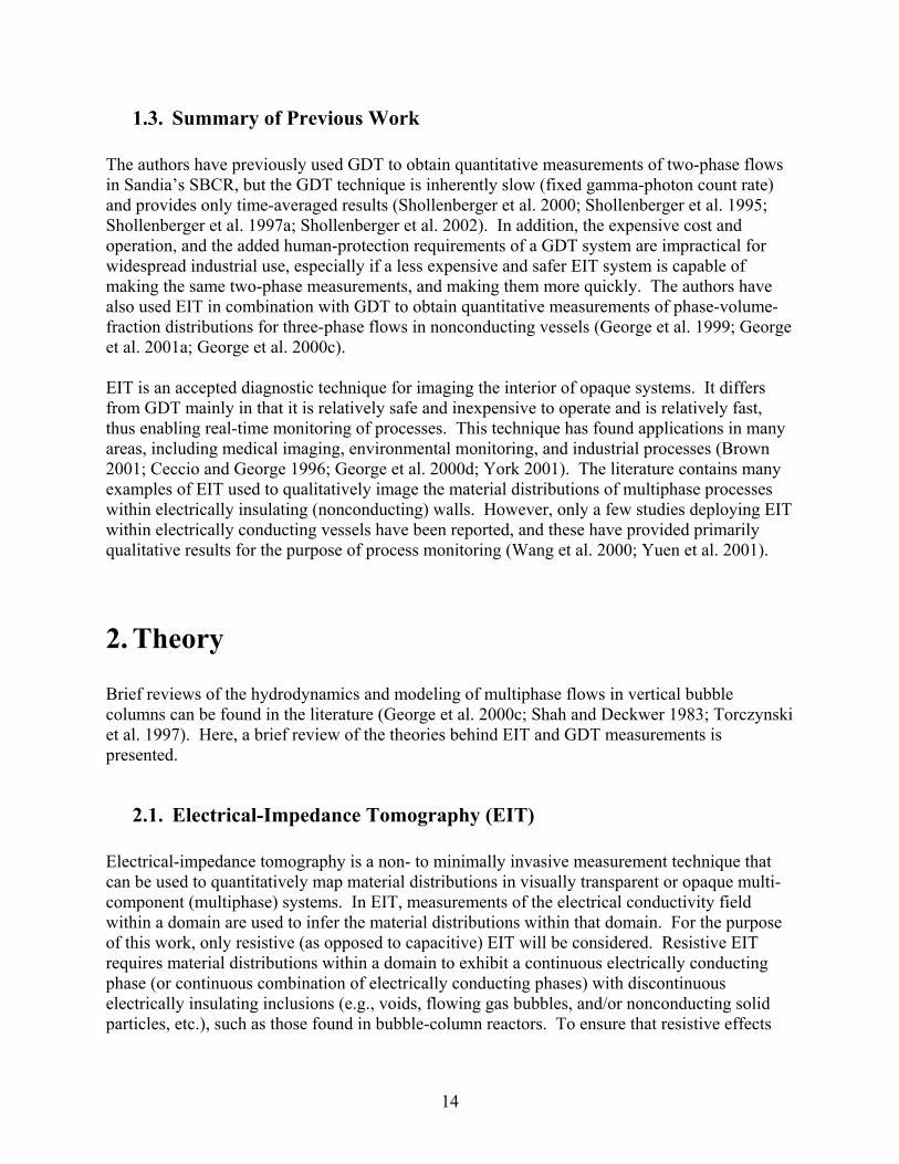
1.3. Summary of Previous Work The authors have previously used GDT to obtain quantitative measurements of two-phase flows in Sandia’s SBCR, but the GDT technique is inherently slow (fixed gamma-photon count rate) and provides only time-averaged results (Shollenberger et al. 2000; Shollenberger et al. 1995; Shollenberger et al. 1997a; Shollenberger et al. 2002). In addition, the expensive cost and operation, and the added human-protection requirements of a GDT system are impractical for widespread industrial use, especially if a less expensive and safer EIT system is capable of making the same two-phase measurements, and making them more quickly. The authors have also used EIT in combination with GDT to obtain quantitative measurements of phase-volume-fraction distributions for three-phase flows in nonconducting vessels (George et al. 1999; George et al. 2001a; George et al. 2000c). EIT is an accepted diagnostic technique for imaging the interior of opaque systems. It differs from GDT mainly in that it is relatively safe and inexpensive to operate and is relatively fast, thus enabling real-time monitoring of processes. This technique has found applications in many areas, including medical imaging, environmental monitoring, and industrial processes (Brown 2001; Ceccio and George 1996; George et al. 2000d; York 2001). The literature contains many examples of EIT used to qualitatively image the material distributions of multiphase processes within electrically insulating (nonconducting) walls. However, only a few studies deploying EIT within electrically conducting vessels have been reported, and these have provided primarily qualitative results for the purpose of process monitoring (Wang et al. 2000; Yuen et al. 2001).
2. Theory Brief reviews of the hydrodynamics and modeling of multiphase flows in vertical bubble columns can be found in the literature (George et al. 2000c; Shah and Deckwer 1983; Torczynski et al. 1997). Here, a brief review of the theories behind EIT and GDT measurements is presented.
2.1. Electrical-Impedance Tomography (EIT) Electrical-impedance tomography is a non- to minimally invasive measurement technique that can be used to quantitatively map material distributions in visually transparent or opaque multi-component (multiphase) systems. In EIT, measurements of the electrical conductivity field within a domain are used to infer the material distributions within that domain. For the purpose of this work, only resistive (as opposed to capacitive) EIT will be considered. Resistive EIT requires material distributions within a domain to exhibit a continuous electrically conducting phase (or continuous combination of electrically conducting phases) with discontinuous electrically insulating inclusions (e.g., voids, flowing gas bubbles, and/or nonconducting solid particles, etc.), such as those found in bubble-column reactors. To ensure that resistive effects
14
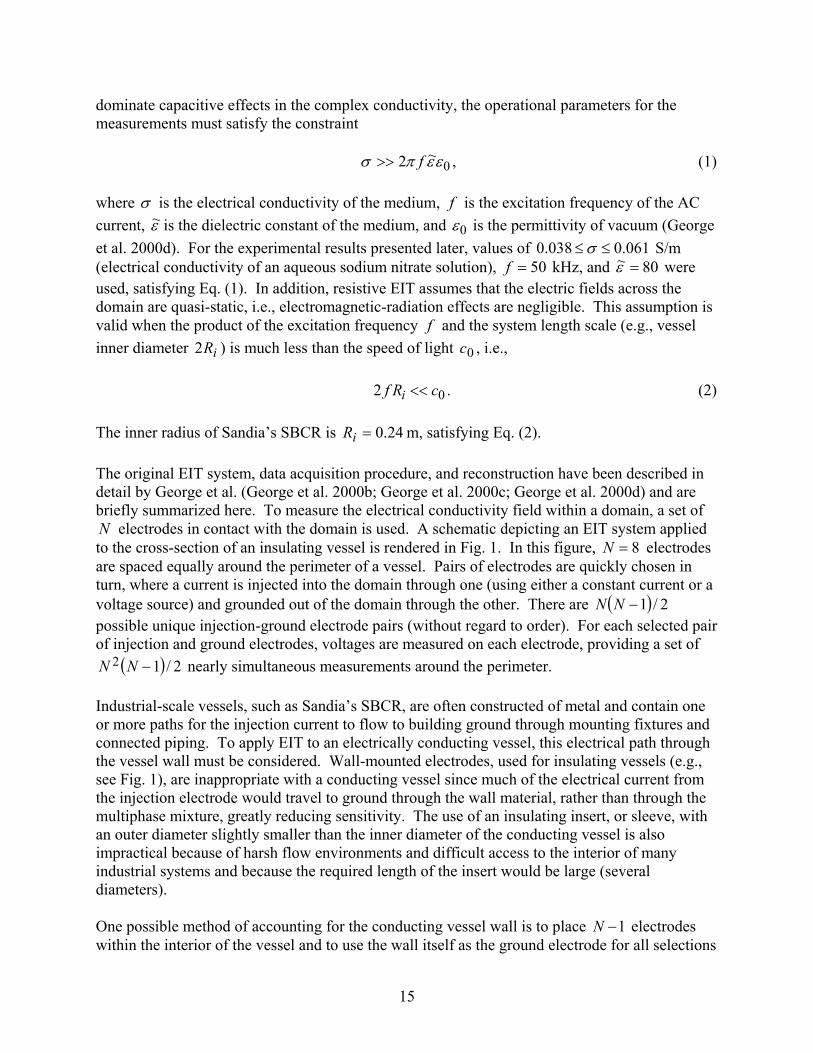
dominate capacitive effects in the complex conductivity, the operational parameters for the measurements must satisfy the constraint
0~2 εεπσ f>> , (1)
where σ is the electrical conductivity of the medium, is the excitation frequency of the AC current,
fε~ is the dielectric constant of the medium, and 0ε is the permittivity of vacuum (George
et al. 2000d). For the experimental results presented later, values of 061.0038.0 ≤≤ σ S/m (electrical conductivity of an aqueous sodium nitrate solution), 50=f kHz, and 80~ =ε were used, satisfying Eq. (1). In addition, resistive EIT assumes that the electric fields across the domain are quasi-static, i.e., electromagnetic-radiation effects are negligible. This assumption is valid when the product of the excitation frequency and the system length scale (e.g., vessel inner diameter ) is much less than the speed of light c , i.e.,
f
iR2 0
02 cRf i << . (2) The inner radius of Sandia’s SBCR is 24.0=iR m, satisfying Eq. (2). The original EIT system, data acquisition procedure, and reconstruction have been described in detail by George et al. (George et al. 2000b; George et al. 2000c; George et al. 2000d) and are briefly summarized here. To measure the electrical conductivity field within a domain, a set of
electrodes in contact with the domain is used. A schematic depicting an EIT system applied to the cross-section of an insulating vessel is rendered in Fig. 1. In this figure, electrodes are spaced equally around the perimeter of a vessel. Pairs of electrodes are quickly chosen in turn, where a current is injected into the domain through one (using either a constant current or a voltage source) and grounded out of the domain through the other. There are possible unique injection-ground electrode pairs (without regard to order). For each selected pair of injection and ground electrodes, voltages are measured on each electrode, providing a set of
nearly simultaneous measurements around the perimeter.
N
2N
8=N
1−NN ( ) 2/
( ) 2/1−N Industrial-scale vessels, such as Sandia’s SBCR, are often constructed of metal and contain one or more paths for the injection current to flow to building ground through mounting fixtures and connected piping. To apply EIT to an electrically conducting vessel, this electrical path through the vessel wall must be considered. Wall-mounted electrodes, used for insulating vessels (e.g., see Fig. 1), are inappropriate with a conducting vessel since much of the electrical current from the injection electrode would travel to ground through the wall material, rather than through the multiphase mixture, greatly reducing sensitivity. The use of an insulating insert, or sleeve, with an outer diameter slightly smaller than the inner diameter of the conducting vessel is also impractical because of harsh flow environments and difficult access to the interior of many industrial systems and because the required length of the insert would be large (several diameters). One possible method of accounting for the conducting vessel wall is to place electrodes within the interior of the vessel and to use the wall itself as the ground electrode for all selections
1−N
15

Figure 1. Schematic of an EIT system applied to an electrically insulating (nonconducting) vessel.
of injection electrode. One means of accomplishing this, which was adopted for this study, is shown schematically in Fig. 2. Here, 71 =−N ring electrodes are wrapped around an electrically insulating rod extended across the diameter of the vessel. Each electrode, in turn, is used to inject current into the domain, while the vessel wall is held at ground, and all of the electrode voltages are recorded. For this system, there are now 1−N possible injection-ground electrode pairs, enabling nearly simultaneous measurements. This system ensures that most of the current crosses the interior of the multiphase flow.
( 1−NN )
Electrical-impedance tomography is generally a noninvasive diagnostic. One drawback of using an internal rod to position the electrodes is that the diagnostic now becomes invasive. For the goal of applying this method inside an SBCR operating in a churn-turbulent regime, a thin rod was expected to have negligible effect on the hydrodynamics due to the robust behavior of bubble column flows (Chen et al. 1999; George et al. 2000c). In addition, EIT measurements are global and reflect the domain between an electrode and ground, not just the local area near the electrode (i.e., near the rod). For these reasons, this application was considered minimally invasive, and the diagnostic was expected to introduce negligible error on the desired measurement. However, the experimental results indicate that this is not the case, but rather suggest that such a cylinder placed across the diameter of the SBCR introduces a nonaxisymmetric disturbance in the flow field, reducing the accuracy in the desired measurement. This is discussed later in the presentation of the experimental results.
16

Figure 2. Schematic of an EIT system applied to an electrically conducting vessel.
In either case of conducting or nonconducting vessel walls, after a set of measurements is obtained for different injection-ground pairs and known injection-electrode currents or voltages, the electrical conductivity field can be reconstructed as follows. The governing equation for the electric potential within the domain, under the constraints of Eqs. (1) and (2), is given by
0=∇⋅∇ Vσ (steady conservation of charge, Ohm’s Law), (3) with boundary conditions
0=+∇⋅ jVσn (Ohm’s Law). (4) Equations (3) and (4) are solved numerically to predict the electrode voltages. In general, the computed conductivity distributions for multiphase flows are not unique. However, a priori information usually exists about the material distributions in many multiphase-flow applications, and a relatively simple function of position and a small set of fitting parameters can be prescribed to provide an accurate representation of the conductivity field σ in the domain. In addition, multiphase flow measurements are often noisy, due to significant temporal fluctuations in the flow. A suitable function describing the conductivity distribution would help to reduce the impact of noise on the results. Based on previous multiphase-flow measurements indicating time-averaged radial-symmetry of fully-developed multiphase flows in bubble columns (George et al. 1998; Shollenberger et al. 1997b), a normalized parabolic radial conductivity distribution was chosen for this study as
17
( )
−
+== 12ˆ1ˆ
1~2
10 il R
rCC
r σσ
σ , (5)
where C and are the fitting parameters and 0ˆ 1C lσ is the measured liquid conductivity. Equation (5) assumes, based on a priori information, that the spatial phase-volume-fraction profiles across the bubble column are suitably and accurately described by a parabolic radial profile. This is not necessarily true in non-fully developed regions of the bubble column (e.g., entrance and disengagement regions) where a quartic or other profile would be a more suitable choice. A finite-element method (FEM) simulation tool capable of modeling Eqs. (3) and (4) is identified and used to predict the electrode voltages for a range of allowable values of the two fitting parameters describing the conductivity distribution in Eq. (5). These results are then stored in a lookup table to facilitate reconstruction of the conductivity distributions from the measurements. An approximate Newton-Raphson method is used to minimize the least-squares difference between the predicted and measured electrode voltages by finding the fitting parameters from the lookup table that provide the best agreement and then interpolating between them. As mentioned, a quartic radial conductivity distribution profile might present a more suitable choice than Eq. (5) by providing an additional degree of freedom (additional fitting parameter). However, such a profile would require a significant increase in the computational time needed to generate the lookup table, and was not pursued for this study owing to budget and time constraints. The resulting description of the conductivity field, reconstructed from the voltage measurements using Eqs. (3)-(5), is then used to infer the phase distributions within the domain using the Maxwell-Hewitt relation (Hewitt 1978; Maxwell 1881)
( ) ( )[ ] ( )( )rr
rEr
g
gg
l αεε
αεσ
σσ+
−===
11
,~ , (6)
along with the requirement of phase conservation
( ) ( ) 1=+ rr lg εε . (7) Here, ( )rgε is the spatial volumetric gas fraction (insulating phase), ( )rlε is the spatial volumetric liquid fraction (conducting phase), and α is an empirical constant. The constant α is equal to 0.5 for stationary three-dimensional insulating inclusions (e.g., suspended spheres) and is equal to 1.0 for two-dimensional insulating inclusions (e.g., parallel cylinders). The gas phase in churn-turbulent bubbly flows is distributed neither as stationary spheres nor as full cylinders. However, a rising bubble in a liquid may be sensed during an EIT measurement as something lying between these two extreme cases because of its vertical motion or axial elongation during the measurement period. Indeed, measurements of two-phase flows in bubble columns demonstrated that 6.0=α provided the best agreement between EIT measurements and
18

corresponding measurements taken using an established GDT system (George et al. 2000d). Therefore, the value of 6.0=α is used for all of the results presented in this study.
2.2. Gamma-Densitometry Tomography (GDT) Gamma-densitometry tomography is an additional noninvasive measurement technique for measuring time-averaged material distributions in visually transparent or opaque multi-component (multiphase) systems that has been used for some time (Chan and Banerjee 1981; Petrick and Swanson 1958; Swift et al. 1978). An established GDT system, measurement, and reconstruction procedure has previously been developed at Sandia (Shollenberger et al. 1997a) and is briefly summarized here. Standard gamma densitometry uses a gamma-radiation source to project a collimated beam of gamma photons through a measurement domain (e.g., bubble column) and to a detector. Gamma scintillations are counted at the detector over a prescribed measurement time for each of the two bounding cases of an empty column and a liquid-filled column, as well as the experimental condition of multiphase flow in the column. The gamma scintillations in the detector (photon arrivals) occur at an unsteady rate that can be well described by the Poisson distribution (Lapp and Andrews 1972). The measurement time, therefore, must be selected to be long enough to enable determination of the gamma-beam intensity (counts/sec) within a prescribed statistical accuracy. As a result, GDT provides inherently time-averaged measurements. Previous studies (George et al. 2000c; Shollenberger et al. 1997a) have found that a measurement time of one-minute allows for a sufficient number of counts to result in a maximum uncertainty of 1% in the count rate (gamma-beam intensity) seen by the detector. A measurement time of one minute was therefore used for this study. Measurements are made of the gamma attenuation, compared to the baselines of a full and empty column, integrated along the beam path, and thus lack spatial resolution. Spatial resolution can be obtained by applying reconstruction techniques to multiple parallel integrated-line measurements when a priori information is available or assumptions are made regarding the phase distribution profiles. As was done for the EIT measurements [see Eq. (5)], an axisymmetric parabolic profile was assumed in this study for the GDT reconstructions. The assumption of an axisymmetric parabolic profile is valid for many vertical multiphase flows when averaged over long time scales (Torczynski et al. 1997). Thus, this is an appropriate assumption for use with GDT since it is an inherently time-averaged measurement. The attenuation of the gamma intensity along a single beam path is related to the attenuation coefficients of the material distributed in the measurement domain (bubble column) along that path by
∑−==
n
iii XII
10 exp µ , (8)
19

where is a reference intensity for the case of no attenuating material between the source and the detector,
0I
iµ is the attenuation coefficient of material slgi ,,= (gas, liquid, solid), and is the cumulative length of attenuating material
iXslgi ,,= along the beam path in the bubble
column. Before reconstructing the volumetric phase distribution in a two-phase gas-liquid flow, parallel line-averaged measurements are taken at various lateral locations x . By taking ratios at each lateral location x of intensities for the multiphase-flow case ( )xI , the liquid-filled column case
, and the gas-filled (empty) column case ( )xIl ( )xI g , the gas-phase and liquid-phase line-
averaged volume fractions, ( )xgε and ( )xlε , respectively, can be determined by
( ) ( ) ( )[ ]( ) ( )[ ]
( )( )
( ) ( )( )xL
xXxLxLxX
xIxIxIxI
x lg
lg
lg
−===
lnln
ε (9)
and
( )( ) ( )[ ]( ) ( )[ ]
( )( )xL
xXxIxIxIxI
x l
lg
gl =−=
lnln
ε , (10)
where is the cumulative length in the gamma-beam path of attenuating material (i.e., the chord length of the beam across the column interior).
( ) ∑= i iXxL
The average attenuation coefficient along a path can be defined as
( ) ( ) ( ) ( )[ ]( ) ( )[ ]
( ) ( )[ ]( ) ( )[ ]xIxI
xIxIxIxI
xIxIxx
lg
gL
lg
lg
n
iii ln
lnlnln
1µµεµµ −== ∑
=, (11)
where ( )xiε is the line-averaged phase volume fraction of each phase i lg,= from Eqs. (9) and (10), and iµ are the known attenuation coefficients of the phases (see Table 4). The line-averaged attenuation coefficient can be normalized as
( )( ) ( ) ( )[ ]
( ) ( )[ ]xIxIxIxIx
xgl
g
gl
g
lnln
=−
−=Ψ
µµ
µµ, (12)
which is noted to be equal to ( )xlε . By assuming an axisymmetric line-averaged gas-phase parabolic distribution in the column [i.e., by curve-fitting Eq. (12)] as
( ) 210 ˆˆ1 xbbx +=Ψ− , (13)
20

a parabolic normalized radial attenuation coefficient distribution can be found by computing the Abel transform of 1 (Vest 1985) as ( )xΨ−
( ) 210 ˆˆ1 raarf +=− µ , (14)
where
( )( )
gl
grrf
µµ
µµµ −
−= . (15)
The radial attenuation coefficient is related to the phase volume fractions, similar to Eq. (11), as
( ) ( ) ( ) ( )rrrr llggn
iii εµεµεµµ +== ∑
=1. (16)
Thus, by noting that the sum of the volume fractions of all present phases must equal unity,
( ) ( ) 1=+ rr lg εε , (17) the radial, time-averaged gas and liquid volumetric phase-fraction profiles are found from
( ) ( ) ( )rrrf lg εεµ =−= 1 . (18)
2.3. Combined EIT and GDT for Three-Phase Measurements Material distributions in three-phase flows in insulating vessels have previously been measured by combining the EIT and GDT techniques (George et al. 2001a). The reconstruction procedure used to make these measurements is reviewed here and is applied to make the three-phase material distribution measurements in electrically conducting vessels presented in this study. To make three-phase material distribution measurements, two complementary measurement techniques must be used. The EIT system functions by distinguishing between conducting and insulating phases (e.g., liquid-gas or liquid-solid for two-phase systems), i.e., it can distinguish the liquid (conducting) phase from all other phases. The GDT system functions by distinguishing between nonattenuating and attenuating phases (e.g., gas-liquid or gas-solid for two-phase systems), i.e., it can distinguish the gas (nonattenuating) phase from all other phases. Through a judicious selection of a solid phase material that has electrically insulating properties similar to those of the gas phase and has gamma-attenuating properties similar to those of the liquid phase, time-averaged three-phase flow material distributions can be determined by noting again that the volume fractions of all present phases must equal unity, i.e.,
( ) ( ) ( ) 1=++ rrr slg εεε . (19)
21

For this study, spherical polystyrene particles, with a nominal diameter of 200 µm were chosen as the solid phase. The properties for this material are listed in Table 4 (Section 4.4). The GDT measurements are made in similar fashion to the procedure outlined for two-phase flows in Eqs. (8)-(15). Since the solid phase is selected to have an attenuation coefficient that is negligibly different from that of the liquid phase, the intensity measurements for the liquid-filled column and empty column are again used as the bounding cases in Eqs. (9)-(12). Here, though, it would be more correct to rewrite Eq. (10) as
( ) ( ) ( )[ ]( ) ( )[ ]
( )( )
( )( )xL
xXxLxX
xIxIxIxI
x ga
lg
ga
−==−=
1lnln
ε , (20)
and Eq. (11) as
( ) ( ) ( ) ( )[ ]( ) ( )[ ]
( ) ( )[ ]( ) ( )[ ]xIxI
xIxIxIxI
xIxIxxlg
ga
lg
lg
n
iii ln
lnlnln
1µµεµµ −== ∑
=, (21)
where the subscript “ ” denotes the gamma-beam “attenuating” material. Next, the Abel transform is applied as before to obtain Eq. (15) for a three-phase flow, and similar to Eq. (16), the radial attenuation coefficient for a three-phase flow is written as
a
( ) ( ) ( ) ( ) ( )rrrrr ssllggn
iii εµεµεµεµµ ++== ∑
=1. (22)
By substituting Eq. (22) into Eq. (15), and then solving for the radial volumetric solid fraction
( )rsε to substitute into Eq. (19), the radial volumetric gas fraction ( )rgε is found as
( ) ( ) ( )rrfr lgs
sl
gs
glg ε
µµµµ
µµ
µµε µ
−−
+
−
−−= 1 . (23)
In Eq. (23), is determined solely from the GDT measurement. EIT measurements
providing a relationship between the two unknowns,
( )rfµ
( )rgε and ( )rlε , are needed for closure. If the gas and solid phases were distributed evenly and had similar morphologies or shapes, then the Maxwell-Hewitt relation [Eq. (6)] could be used directly to obtain
( ) ( )( )rrrg σα
σε ~1
~1+−
= . (24)
The solid phase, however, consists of spherical particles with a small size distribution nominally around 200 µm, while the gas phase consists of non-spherical bubbles and gas slugs with a different, wider size distribution. To account for these two different size distributions, a
22

recursive, bimodal application of the Maxwell-Hewitt relation was suggested (George et al. 2001a) and was used for the three-phase results presented in this study. The bimodal application of the Maxwell-Hewitt relation assumes that the solid phase is evenly distributed everywhere within the liquid phase, such that the liquid-solid mixture can be considered as a single medium in which the gas phase is distributed. This assumption is valid when the average size of solid phase particles is small compared to the average size of gas phase masses and the solid phase can be well mixed (lofted) in the liquid phase. This recursive formulation first applies the Maxwell-Hewitt relation [Eq. (6)] to consider the conductivity ratio of the liquid-solid mixture to the pure liquid as
( ) ( )( )
( )( )
( )( )
( )( )r
rr
r
rr
Err
Er
g
s
g
s
g
s
ls
s
l
lslls
εε
α
εε
αε
εα
εε
σσ
σ
−+
−−
=
−=
==
11
11
,1
,~, . (25)
Next, this formulation applies the Maxwell-Hewitt relation [Eq. (6)] to consider the conductivity ratio of the three-phase flow to the liquid-solid mixture as
( )( ) ( )[ ] ( )
( )rr
rEr
r
g
gg
lslsgls αε
εαε
σσσ
+
−===
11
,~, . (26)
Then, by multiplying Eq. (25) with Eq. (26), the ratio of the reconstructed (i.e., measured) three-phase conductivity distribution to the reconstructed (i.e., measured) liquid conductivity distribution can be related to the two insulating volumetric phase fractions, ( )rgε and ( )rsε , as
( ) ( )( )
( ) ( )( )
( ) ( )( ) ( )
+−
−−
+
−=
==
rrrr
rrr
rrr
sg
sg
g
g
l
ls
lsl αεε
εε
αε
ε
σσ
σσ
σσσ
11
11~ . (27)
Using Eqs. (19) and (27), the required relation for closure of Eq. (23) is found, i.e.,
( ) ( )[ ]ασεε ,~,rfr gl = . (28) Note that the conductivity of the solid-liquid mixture need not be measured experimentally. After substituting Eq. (22) into Eq. (15), Eqs. (15), (23), and (28) must be solved simultaneously to determine the gas volume fraction. A closed-form solution was previously reported (George et al. 2001a) and is repeated here with a correction of the sign preceding the square root in Eq. (28):
( ) ( ) ( ) ( ) ( )( )ra
rcrarbrbrg 2
42 −−−=ε , (29)
23

where
( ) σαµµµµ
αµµµµ ~1 2
−
−−
−−
+=gs
gl
gs
lsra ,
( ) ( )[ ] σαµµµµ
αµµµµ
µµµµ
µ~12 2
−
−
−+−
−−
+
−
−+−= rfrb
gs
gl
gs
ls
gs
gl ,
( ) ( ) ( )[ ] σαµµµµ
µµµµ
µµµµ
µµ~11 2
−
−
−+
−−
−+
−
−−= rfrfrc
gs
gl
gs
ls
gs
gl .
The liquid volume fraction is then found from Eq. (23) using the gas volume fraction ( )rgε from
Eq. (29) and the reconstructed normalized radial attenuation coefficient from Eq. (15). The solid volumetric fraction is then found from Eq. (19).
( )rfµ
The numerical codes (written in FORTRAN77) used to implement the reconstructions for this study are provided in the appendix.
3. Diagnostic Systems
3.1. EIT Apparatus As was mentioned, an existing EIT system, originally developed for use with nonconducting vessels, was modified for this study. The original system has previously been described in detail (George et al. 2000c). Here, a brief overview of the system is presented with discussion on the modifications that were made to enable deployment in metal vessels. A photograph of the EIT system is shown in Fig. 3 along with a metal vessel that was used to make benchtop proof-of-concept measurements. The benchtop measurements are discussed later. The EIT system consists of an electronics box, computer-controlled data acquisition hardware and software, a frequency signal generator, and an electrode array. The electrode array chosen for this study consists of seven discrete electrodes positioned along an insulating rod, which is capable of spanning the interior diameter of the SBCR (see, for example, Fig. 2). Seven sets of two miniature coaxial cables are used to transmit high-fidelity voltage signals between the generating electronics and the seven rod electrodes. These cables pass through small holes drilled in the wall of the rod (the holes are subsequently sealed) and are screwed to tabs on the underside of the corresponding electrodes. An eighth set of coaxial cables is available to attach to the exterior of the metallic vessel, which serves as the ground electrode.
24

Figure 3. Photograph of verification experiment showing the EIT electronics, the electrode rod with seven copper ring electrodes (the top eighth ring shown is a plastic seal), and the standpipe.
The electronics box is an in-house developed system that consists of a constant voltage source, a voltage ground, an excitation multiplexer to apply the constant voltage (inject current) and ground to the proper electrodes, an erasable programmable read-only memory chip (EPROM) to control the sequence of the multiplexer, another EPROM and multiplexer to measure the voltages on each electrode for each injection-ground pair, and measurement and control electronics. The measurement electronics include an instrumentation amplifier, phase-sensitive demodulators, low-pass filters to reduce high frequency noise, and a data acquisition/digital control card. Pictures of the electronics box internals are shown in Fig. 4. The major modifications made for this study included the replacement of hardwired electrode-excitation and measurement sequencing circuits with programmable EPROMs, the replacement of a constant current source with a constant voltage source, and the added capability to measure the current going to the injection electrode. The measurement sequence is as follows. A constant voltage is applied to an electrode located on the rod, and the vessel wall is grounded. The voltage on each electrode is measured in turn, with the current passing through the injection electrode measured after each individual electrode
25

Figure 4. Photographs of the circuits boards inside the EIT electronics box.
voltage measurement. The constant voltage is then applied to the next electrode on the rod and the sequence of voltage and current measurements is repeated. This continues until all electrodes on the rod have served as the injection electrode, resulting in ( )1−NN voltage and current measurements. One hundred sets of these 56 measurements are recorded and then averaged. These averaged voltage and current measurements are then used to reconstruct the electrical conductivity field as described in Chapter 2.
3.2. GDT Apparatus As was mentioned, an established GDT system previously has been developed at Sandia (Shollenberger et al. 1997a). This system was first used in this study to validate the EIT measurements of the material distributions in the SBCR for two-phase flows, and subsequently it was combined with EIT to make measurements of the material distributions in three-phase flows. A schematic of the GDT system used in this study is shown in Fig. 5. This system consists of a 5-curie 137Cs gamma source (gamma photon energy of 0.662 MeV), a sodium iodide (NaI) scintillation detector system, a computer-controlled traverse, and a computer data acquisition system. The source and detector are both lead-shielded and are mounted on opposing arms of a two-axis traverse. The separation between the source and detector is sufficient to accommodate vessels up to 0.66 m outer diameter. The source and detector move in tandem along a horizontal traverse with a range of approximately 0.6 m of automated travel. The horizontal traverse, itself, is mounted on a vertical traverse with approximately 3 m of automated travel. The traverses operate with a positioning accuracy of 0.1 mm.
26

computer-controlled heavy-duty traverse with 0.6 m horizontal and 3 m vertical travel
Scintillation detector:NaI (Tl) crystal,photomultiplier,
preamplifier5 curie, 137Cs
source:0.662 MeV
photon beam
high voltagepower supply
multi-channelanalyzer
spectroscopyamplifier
analog-to-digitalconverter
PC-based dataacquisition andcontrol system
Figure 5. A schematic of the GDT system in the horizontal plane.
4. Experiments
4.1. Benchtop Validation Test A study verifying the feasibility of using the wall of an electrically conducting vessel as ground was completed (Liter et al. 2002). The results of this study are summarized here. To verify that the EIT system would provide accurate results using the wall as ground, prior to implementation on Sandia’s SBCR, a simple verification experiment was devised to provide a one-dimensional (vertical) step-variation in electrical conductivity, resulting in two electrically differentiable regions. This experiment is schematically shown in Fig. 6. A photograph of the various components of the experiment is shown in Fig. 4. The electrode rod used for the benchtop test is fabricated from a PVC tube with a 2.2-cm OD and a 1.5-cm ID. Two sets of electrodes were used for the experiment. Each set consisted of 7 ring
27

Figure 6. Schematic of verification experiment consisting of an electrode rod inserted coaxially in an electrically conducting standpipe filled with nonconducting solid polystyrene particles and liquid.
electrodes, one set made from 0.04-mm thick copper foil, and the other from 0.07-mm thick stainless steel 304 foil. All other dimensions are the same. The electrodes are 2.54 cm in length and are wrapped around the rod with a 3.5-cm edge-to-edge separation between them. When the rod is inserted into the standpipe, the distance between the bottom electrode and the base of the standpipe is 7.0 cm. The liquid level is kept at 7.0 cm above the top electrode to maintain vertical symmetry. Electrode ground wires are attached to the vessel exterior.
lh
The particle bed consists of polystyrene spheres, of diameter 3=pd mm, allowed to fall through the water into random packing. The particles are subsequently stirred to remove trapped air bubbles, and then the particle-bed surface is planed flat. A metal cylinder, or standpipe, of inner diameter 7.14=d
bh
cm with an electrically insulating base is used as the vessel (ground electrode). The electrode rod is positioned coaxially inside the standpipe. The standpipe is filled to various heights with solid particles and a liquid (water with a small amount of aqueous sodium nitrate added to control the liquid conductivity),
28

resulting in a region of lower conductivity in the saturated particle bed, and a region of higher conductivity in the liquid above the bed. To verify the use of EIT on a conducting vessel, with the vessel used as ground, various heights of the particle bed were predicted using the EIT system, and then compared with direct measurements made using a meter stick. These measurements are presented in Chapter 5.
4.2. Sandia’s Slurry Bubble-Column Reactor (SBCR) Facility After the EIT system was proven capable of accurately measuring material distributions in static multiphase systems, it was deployed on the SBCR shown in Fig. 7. The SBCR facility at Sandia has previously been described in detail (George et al. 2000a; Shollenberger et al. 2000). A brief
Figure 7. Photograph of the Sandia slurry bubble-column reactor facility. Also shown is the vault for the gamma source mounted on the two-axis automated traverse.
29

description of the SBCR facility is presented here. The SBCR is comprised of a stainless steel column that has a 0.48 m inner diameter, 13 mm thick sidewalls, and an internal height of 3.15 m. The column is rated for temperatures up to 200 ºC and headspace pressures up to 689 kPa gauge. Volumetric airflow rates into the column of up to 55 L/s corresponding to superficial gas velocities up to 30 cm/s are possible. The column contains 24 instrumentation/view ports located at six different levels spaced 45.7 cm apart. Air is injected into the bottom of the bubble column from a high-pressure air supply through a cross sparger (air injector). The picture of a similar cross sparger (this one with upward-facing holes) to that used for this study is shown in Fig. 8. The cross sparger used has 96 downward-facing holes (1.55 mm-diameter) distributed along the sparger pipes. The resulting porosity for gas injection is 0.1%. The holes on the sparger are located 0.157 m (0.33 diameters) above the internal vessel bottom. The SBCR has been used with both water and mineral oil (Shollenberger et al. 2002). For this study, deionized water was used as the working fluid with a fill-height in the SBCR of 1.93 m (4 diameters) from the internal vessel bottom. Small amounts of sodium nitrate were added to the water to control the water electrical conductivity. The EIT electrode rod used in the SBCR is of the same general design as the one used in the benchtop experiment, with a few differences. The rod is fabricated from a garolite tube with a 1.91-cm OD and a 0.95-cm ID. The electrodes are made from 0.1-mm thick stainless steel shim stock and are 3.18 cm in length. They are wrapped around the rod and seated in a machined out band such that the surfaces of the rod and electrode are flush. The electrodes are placed along the rod with a 3.18-cm edge-to-edge separation. The rod is installed in the SBCR through the third level of instrumentation ports at a rod-center-axis height of 1.34 m above the internal vessel bottom, or 1.19 m above the sparger holes. Figure 9 schematically shows the electrode rod deployed in the SBCR. Also shown in Fig. 9, in the bottom left corner, are hypothetical voltage contour lines corresponding to two different values of the electrical conductivity distribution.
Figure 8. Photograph of a cross sparger similar to that used in this study to inject air into the bottom of the bubble column.
30

Figure 9. Schematic of EIT system applied to Sandia’s slurry bubble-column reactor (SBCR). Shown on the right is a photograph of the SBCR (0.48-m ID). The bottom left shows predictions of voltage contours in a cross-section of the SBCR for two cases, one of constant conductivity in the top half, and one of variable conductivity in the bottom half.
For both cases, electrode 3 is selected as the current injection electrode. The top half of the figure shows voltage contours for an assumed constant electrical conductivity σ across the domain. The bottom half of the figure shows voltage contours for an assumed parabolic electrical conductivity distribution ( )rσ across the domain. As can be seen, the electrode voltages are distinguishable for each case.
31

4.3. Experimental Procedure for Measurements in Sandia’s SBCR Quantitative measurements of the phase volume phase fractions were made in Sandia's SBCR for two- and three-phase flows, at the operating conditions listed in Table 3, using the following procedure. Before measurements are recorded, the column pressure and gas flow rate are set to the desired levels and the SBCR is allowed to operate for at least 30 minutes to allow the operating conditions and liquid temperature to stabilize. The column pressure and gas flow rate are then adjusted as needed. Once a desired stable operating condition is obtained, the GDT system is employed to measure line-averaged intensities at 2 vertical locations, 11.43 cm above, and 11.43 cm below the center of the third level of instrumentation ports (above and below the instrumentation ports containing the EIT electrode rod). At each height, 11 GDT measurements are taken at 4.0-cm intervals in the horizontal plane, equally spaced from –20.0 cm to 20 cm relative to the column center. Thus, one set consists of 22 GDT measurements. Each GDT measurement requires 60 seconds resulting in a total measurement time for each set on the order of 30 minutes. The operating conditions are continuously monitored during the measurements to ensure there are no significant changes in column pressure and gas flow rate. These 22 GDT measurements are then repeated for the case of no gas flowing in the column (liquid)
Table 3. Operating conditions for the two- and three-phase tests in the SBCR.
Test Number
Column Pressure,
KPa (psig)
Superficial Gas Velocity,
cm/s
Liquid Conductivity,
µS/cm
Nominal Solids loading,
% volume Two-Phase Tests
1 103 (15) 10 420 - 2 103 (15) 15 409 - 3 103 (15) 20 420 - 4 103 (15) 25 386 - 5 207 (30) 10 403 - 6 207 (30) 15 419 - 7 207 (30) 20 407 - 8 207 (30) 25 407 - 9 310 (45) 10 420 - 10 310 (45) 15 418 - 11 310 (45) 20 418 -
Three-Phase Tests 1 103 (15) 10 609 0 2 207 (30) 10 609 0 3 103 (15) 10 412 4 4 207 (30) 10 412 4 5 103 (15) 10 652 8 6 207 (30) 10 652 8
32

and the case of an empty column (no liquid) to provide the bounding conditions needed for reconstruction of the material distributions as detailed in Chapter 2. EIT measurements are recorded, using a different computer, during the collection of the GDT measurements for both the gas-flowing case, and the liquid-only case [used to normalize Eq. (5)]. One hundred sets of voltages are recorded, and the measurements are then time-averaged. The reconstruction of the conductivity distribution from the time-averaged, measured EIT electrode voltages utilizes an FEM simulation of the SBCR. A computational mesh on which voltage fields are computed is shown in Fig. 10(a). This mesh corresponds to one-quarter of the interior of the SBCR with the electrode rod inserted along a diameter. Symmetry is presumed on the two planar surfaces that intersect the electrode rod. The seven internal electrodes, which appear as notches on the rod, are modeled as regions of high conductivity [~1000 times the liquid value (George et al. 2000d)] and have outer surfaces that are flush with the outer diameter of the rod. In this case, the electrodes have equal lengths and edge-to-edge separations of
(a) (b)
Figure 10. (a) Computational mesh corresponding to one-quarter of the interior of the SBCR with the EIT rod inserted along a diameter. (b) Voltage contours computed for a uniform electrical conductivity throughout the domain with current injection from electrode 4.
33

3.18 cm, and the outer diameter of the electrodes and the rod are 1.91 cm, modeling the garolite electrode rod used in the SBCR experiments. Example voltage contours computed on this mesh (see Section 2.1) using an FEM simulation tool [FIDAP (Fluent 1998)] are shown in Figure 10(b). In this particular case, a uniform liquid conductivity is used (corresponding to the case of no gas flowing, i.e., the liquid-filled column), and current is injected from electrode 4 before exiting the domain through the grounded vessel wall. Additional calculations for injection from other electrodes and for spatially varying conductivity fields have been performed to create a lookup table facilitating reconstruction of the conductivity distribution (and subsequently the material distributions) from the experimental voltage and current measurements, as discussed in Section 2.1. For the three-phase measurements, some additional considerations are needed. First, EIT measurements of the liquid in the column must be taken to provide a normalizing baseline for the reconstruction of the electrical conductivity distribution. The solid particles, once mixed with the liquid and flowing gas, require approximately one hour to settle out of suspension in the liquid once the gas flow has stopped. During this time, the water temperature may rise from the stable operating condition and thus change the liquid conductivity. Second, the particles arrived from the supplier with an anti-static coating that behaves as a surfactant when dissolved in water. All of the solid particles used in the experiment were repeatedly rinsed and strained, but residual surfactant remained. This residual surfactant dissolves into the liquid during operation of the SBCR and can significantly change the liquid conductivity. Moreover, this added surfactant can change the liquid-gas interfacial surface tension, possibly altering the bubble-column hydrodynamics. Therefore, a meaningful comparison cannot be made between two-phase flow measurements using just air and water and three-phase flow measurements where the water now contains a surfactant. To enable a comparison between two- and three-phase measurements, a 0% solids loading case is examined in which the solid particles are strained out of the liquid from a three-phase flow condition, and the liquid (with surfactant, etc.) is then returned to the SBCR. To account for the loss of volume of the solid, makeup water with a little sodium nitrate is added to restore the liquid level to the proper fill-height and to control the liquid conductivity. Since this new two-phase flow utilizes liquid similar to that used in the three-phase measurements, and since there is no required waiting period to allow solid particles to settle out of suspension, baseline liquid-only EIT measurements were made for the 0% loading case and used for all six of the three-phase flow measurement reconstructions. As will be discussed later, this assumption was not a good one and introduced large errors in the reconstructed conductivity distribution ratios.
4.4. Experimental Material Properties The relevant properties for the phase materials used in this study are listed in Table 4 and were obtained from a previous study at Sandia using the GDT and EIT systems to make three-phase measurements in insulating vessels (George et al. 2001a). Polystyrene was chosen for the solid phase because it possessed a density near that of the liquid, thus providing good mixing and lofting characteristics, and it possessed attenuating properties similar to that of the water and electrical properties similar to that of the air, which was required to enable GDT and EIT to be
34

Table 4. Properties of the phase materials used for the material distribution reconstructions.
Material Density, ρ (g/cm3)
Attenuation Coefficient, µ (cm-1)
Conductivity, σ (µS/cm)
air - 0.0000819 ~10-10 water/NaNO3 0.997 0.0856 386-609 polystyrene 1.04 0.0866 <10-10
combined as described in Chapter 2. The density for the air that would correspond to the measurements is a function of the headspace column pressure and the height of liquid above the electrode rod. Since it is not required for reconstruction of the phase distributions, it is not listed in Table 4.
4.5. Sources of Uncertainty The uncertainties in the bulk-averaged gas volume fraction measurements performed on the SBCR using the established GDT system have previously been described (Shollenberger et al. 1997a) and determined to be near ±0.4% deviation in magnitude for line-averaged gas volume fractions greater than 8%. This system was used as the standard reference for the two-phase flow EIT measurements. Previous studies (George et al. 2000c) have examined the effect of uncertainties in the measured electrode voltages on the reconstructed material phase distributions for the original EIT system used with insulating vessels. The determined uncertainty of 0.7% is expected to be similar for the modified EIT system if a quartic profile is used in the reconstruction and if the electrode array is positioned to be noninvasive around the flow domain. Since this study used a parabolic profile, the uncertainty due to profile shape is expected to be slightly higher. In addition, a larger source of uncertainty is expected in this study because the electrode rod used in the SBCR is invasive to the flow field. The reconstruction of the conductivity distribution, using the EIT measured voltages, assumes a radial axisymmetric and smooth parabolic profile for the phase distributions, a fair assumption for time-averaged fully-developed churn-turbulent multiphase flows (George et al. 2000d; Shollenberger et al. 1997a; Torczynski et al. 1997). The electrode rod design used in this study was initially chosen assuming it would have a negligible effect on the hydrodynamics of a churn-turbulent flow in a bubble column. This assumption was based on a published study addressing the effect of internal structures on bubble column hydrodynamics (Chen et al. 1999). If a significant liquid boundary layer develops around the rod, and a wake develops behind the rod, then the parabolic profile assumption is no longer valid. This is believed to be the case for some of the results presented here. Where an internal structure might have a negligible effect on the global bulk-averaged hydrodynamics, the experimental results indicate a non-negligible effect on the local hydrodynamics immediately in
35

the vicinity of the rod. More study characterizing and quantifying the uncertainty of an invasive electrode rod is required.
5. Experimental Results and Discussion
5.1. Benchtop Validation Measurements The EIT system was first used in a solid-liquid bench-top experiment to measure the height of a packed bed in a liquid-filled standpipe as described in Section 4.1. Comparisons of the results versus particle-bed heights as directly measured by a meter stick are shown in Fig. 11, and their numerical values are given in Table 5. Measurements for six different bed heights are presented, three using copper electrodes and three using stainless steel 304 electrodes. For each bed height, at least 20 sets of voltage measurements were taken, the average of which was used in the numerical reconstruction (prediction). Based on previous applications of the EIT system to quantitatively measure conductivity distributions in an insulating vessel and its validation through comparison with gamma densitometry tomography (GDT) (George et al. 2000c; George et al. 2000d), the error in the reconstructed bed height is estimated to be ±0.3 cm. The particle-bed height h was also determined by using a meter stick to directly measure the distance from the top of the particle bed to the top of the standpipe. The total standpipe height
b
05
10152025303540
0 5 10 15 20 25 30 35 40
Copper ElectrodesSS ElectrodesPr
edic
ted
Bed
Hei
ght,
cm
Measured Bed Height, cm
Figure 11. Plot of the EIT reconstructed particle-bed height versus the measured particle-bed height in the steel standpipe.
36

Table 5. Measured and predicted particle-bed heights for 6 different tests, 3 with copper electrodes and 3 with stainless steel electrodes.
Electrode Material Measured Height, cm Predicted Height, cm % difference 20.3 20.6 1.5 26.4 26.2 0.8
Copper
36.2 36.1 0.3 11.7 12.4 6.0 24.1 24.6 2.1
Stainless Steel
36.5 36.3 0.5 Uncertainty ±0.7 ±0.3
minus the measured distance equals the particle-bed height. Two main sources of error were present in this measurement. One, flatness of the surface of the particle-bed was difficult to obtain at depth inside the standpipe and variations in the height across the surface were present. Two, the meter stick is believed to have possibly penetrated into the top of the particle bed, resulting in a measurement smaller than the actual bed height. To mitigate these errors, measurements were taken at various locations across the surface and averaged. The error in the measured bed height is estimated to be ±0.7 cm. As can be seen, all of the measurements agree within experimental uncertainties and therefore are said to exhibit good agreement. For the cases of particle-bed heights less than 25 cm, the EIT predictions appear to be slightly larger than the measurements. For the smaller bed heights, the meter stick used to measure the height is required to be inserted deeper into the standpipe. The associated error of the meter stick penetrating through the bed surface is potentially larger since it is more difficult to discern when the meter stick actually comes in contact with the surface. Therefore, the potential error between the measured bed height and the actual bed height is expected to increase with decreasing bed height, with the measured bed height being less than the actual value. This is consistent with the results shown in Figure(George et al. 2001b) 11.
5.2. Two-Phase Measurements After the benchtop tests proved the vessel wall could be used as a permanent ground electrode to make EIT measurements of material distributions in metal vessels, the EIT system was deployed on the SBCR to make two-phase measurements. One hundred sets of electrode voltage measurements were recorded and then averaged at the 11 different test conditions listed in Table 3. All EIT measurements were taken at a single vertical height through the center of the third level of instrumentation ports on the SBCR. The gas-volume-fraction distribution EIT measurements were compared against results from an established GDT system that was used to measure the volumetric gas volume fractions at just above and just below the instrumentation ports. The two GDT distribution results were averaged to estimate the gas-volumetric-fraction distribution in the same plane as the EIT results.
37

Numerical values for the centerline, sidewall, and bulk-averaged gas volume fractions for the EIT and averaged GDT measurements are given in Table 6 along with their percent differences. The results for the measured gas-volume-fraction distributions are presented in Figs. 12-22. As can be seen from the percent difference in bulk-averaged gas volume fractions listed in Table 6, all of the EIT results predict gas volume fractions less than that of the GDT measurements. One possible explanation is due to the electrode rod being invasive to the flow field. As was mentioned, a liquid-rich (relative to the bulk flow) annulus might be developing with the boundary layer around the rod. This would bias the EIT electrodes into sensing a lower gas volume fraction. This effect is somewhat mitigated (with distance from the ground electrode, or wall) by the fact that EIT measurements are global in nature, since the measured voltages are the result of the injection current having to travel across the flow domain between the injection and ground electrodes. A nonaxisymmetric liquid annulus spanning the diameter of the column along the rod would create a biased path (path of less resistance) for the current to travel to the vessel wall (ground). This effect would be greatest near the wall and would decrease near the center of the column (lowest gas volume fraction near the wall), which is consistent with 7 of the 11 measurements taken. The remaining four measurements (Tests 2, 4, 9, and 11) do not strongly exhibit this effect, but rather show good agreement between the GDT and EIT measurements. One explanation for the good agreement found in these four tests could be that large or numerous gas masses enveloped parts of the rod coincident to the measurements of the electrode voltage sets, reducing the effect of the liquid annulus. There is currently no explanation for why this occurred in only four of the 11 cases. Further testing and examination is required. The GDT results for the bulk-averaged gas volume fraction are graphically presented in Fig. 23. The bulk-averaged gas volume fraction is shown to monotonically increase with increasing
Table 6. Comparison of EIT and averaged GDT measurements of gas volume fractions for the 11 different two-phase operating conditions listed in Table 4.
Centerline, 0=iRr Sidewall, 1±=iRr Bulk-averaged Test No.
Fig. No. EIT GDT %Diff. EIT GDT %Diff. EIT GDT %Diff.
1 12 0.259 0.271 4.3 0.002 0.102 97.8 0.158 0.208 23.8 2 13 0.322 0.325 0.8 0.123 0.123 -0.1 0.241 0.250 3.38 3 14 0.367 0.380 3.0 0.026 0.131 80.2 0.233 0.288 19.0 4 15 0.435 0.432 -0.7 0.174 0.172 -0.0 0.327 0.336 2.6 5 16 0.293 0.306 5.1 0.021 0.161 87.0 0.186 0.252 26.0 6 17 0.314 0.371 15.4 0.026 0.180 85.3 0.202 0.300 32.7 7 18 0.422 0.420 -0.3 0.149 0.200 25.2 0.316 0.338 6.6 8 19 0.443 0.473 6.4 0.126 0.249 49.3 0.319 0.390 18.3 9 20 0.320 0.319 -0.4 0.187 0.196 4.4 0.268 0.274 2.2 10 21 0.382 0.407 6.2 0.074 0.214 65.5 0.261 0.335 22.2 11 22 0.454 0.461 1.5 0.248 0.246 -0.0 0.369 0.381 3.3
38

superficial gas velocity and decrease with increasing column pressure, consistent with previous results for two-phase flow measurements (George et al. 2000d; Shollenberger et al. 2002). The EIT results for the bulk-averaged gas fraction are graphically presented in Fig. 24. Here, the results are qualitatively similar to the GDT results in magnitude and trends, however, the monotinicity in the trends is no longer present. By comparing Figs. 23 and 24, the variations in the percent difference between the GDT and EIT results can clearly be seen.
0
0.1
0.2
0.3
0.4
0.5
-1 -0.5 0 0.5 1
EITGDT, aboveGDT, below
Gas
Vol
ume
Frac
tion
Normalized Radial Position
ug = 10 cm s-1
pcol = 103 kPa
Figure 12. Comparison of symmetric radial gas volume fraction profiles from EIT and GDT for a column pressure 103 kPa and a superficial gas velocity 10 cm/s. =colp =gu
0
0.1
0.2
0.3
0.4
0.5
-1 -0.5 0 0.5 1
EITGDT, aboveGDT, below
Gas
Vol
ume
Frac
tion
Normalized Radial Position
ug = 15 cm s-1
pcol
= 103 kPa
Figure 13. Comparison of symmetric radial gas volume fraction profiles from EIT and GDT for a column pressure 103 kPa and a superficial gas velocity 15 cm/s. =colp =gu
39

0
0.1
0.2
0.3
0.4
0.5
-1 -0.5 0 0.5 1
EITGDT, aboveGDT, below
Gas
Vol
ume
Frac
tion
Normalized Radial Position
ug = 20 cm s-1
pcol
= 103 kPa
Figure 14. Comparison of symmetric radial gas volume fraction profiles from EIT and GDT for a column pressure 103 kPa and a superficial gas velocity 20 cm/s. =colp =gu
0
0.1
0.2
0.3
0.4
0.5
-1 -0.5 0 0.5 1
EITGDT, aboveGDT, below
Gas
Vol
ume
Frac
tion
Normalized Radial Position
ug = 25 cm s-1
pcol
= 103 kPa
Figure 15. Comparison of symmetric radial gas volume fraction profiles from EIT and GDT for a column pressure 103 kPa and a superficial gas velocity 25 cm/s. =colp =gu
40

0
0.1
0.2
0.3
0.4
0.5
-1 -0.5 0 0.5 1
EITGDT, aboveGDT, below
Gas
Vol
ume
Frac
tion
Normalized Radial Position
ug = 10 cm s-1
pcol
= 207 kPa
Figure 16. Comparison of symmetric radial gas volume fraction profiles from EIT and GDT for a column pressure 207 kPa and a superficial gas velocity 10 cm/s. =colp =gu
0
0.1
0.2
0.3
0.4
0.5
-1 -0.5 0 0.5 1
EITGDT, aboveGDT, below
Gas
Vol
ume
Frac
tion
Normalized Radial Position
ug = 15 cm s-1
pcol
= 207 kPa
Figure 17. Comparison of symmetric radial gas volume fraction profiles from EIT and GDT for a column pressure 207 kPa and a superficial gas velocity 15 cm/s. =colp =gu
41

0
0.1
0.2
0.3
0.4
0.5
-1 -0.5 0 0.5 1
EITGDT, aboveGDT, below
Gas
Vol
ume
Frac
tion
Normalized Radial Position
ug = 20 cm s-1
pcol
= 207 kPa
Figure 18. Comparison of symmetric radial gas volume fraction profiles from EIT and GDT for a column pressure 207 kPa and a superficial gas velocity 20 cm/s. =colp =gu
0
0.1
0.2
0.3
0.4
0.5
-1 -0.5 0 0.5 1
EITGDT, aboveGDT, below
Gas
Vol
ume
Frac
tion
Normalized Radial Position
ug = 25 cm s-1
pcol
= 207 kPa
Figure 19. Comparison of symmetric radial gas volume fraction profiles from EIT and GDT for a column pressure 207 kPa and a superficial gas velocity 25 cm/s. =colp =gu
42

0
0.1
0.2
0.3
0.4
0.5
-1 -0.5 0 0.5 1
EITGDT, aboveGDT, below
Gas
Vol
ume
Frac
tion
Normalized Radial Position
ug = 10 cm s-1
pcol
= 310 kPa
Figure 20. Comparison of symmetric radial gas volume fraction profiles from EIT and GDT for a column pressure 310 kPa and a superficial gas velocity 10 cm/s. =colp =gu
0
0.1
0.2
0.3
0.4
0.5
-1 -0.5 0 0.5 1
EITGDT, aboveGDT, below
Gas
Vol
ume
Frac
tion
Normalized Radial Position
ug = 15 cm s-1
pcol
= 310 kPa
Figure 21. Comparison of symmetric radial gas volume fraction profiles from EIT and GDT for a column pressure 310 kPa and a superficial gas velocity 15 cm/s. =colp =gu
43

0
0.1
0.2
0.3
0.4
0.5
-1 -0.5 0 0.5 1
EITGDT, aboveGDT, below
Gas
Vol
ume
Frac
tion
Normalized Radial Position
ug = 20 cm s-1
pcol
= 310 kPa
Figure 22. Comparison of symmetric radial gas volume fraction profiles from EIT and GDT for a column pressure 310 kPa and a superficial gas velocity 20 cm/s. =colp =gu
0.1
0.2
0.3
0.4
10 15 20 25
103 kPa207 kPa310 kPa
Bul
k G
as V
olum
e Fr
actio
n
Superficial Gas Flow Rate, cm/s
Figure 23. Plot of the bulk-averaged gas fraction as a function of superficial gas velocity and column pressure, from GDT measurements.
44

0.1
0.2
0.3
0.4
10 15 20 25
103 kPa207 kPa310 kPa
Bul
k G
as V
olum
e Fr
actio
n
Superficial Gas Flow Rate, cm/s
Figure 24. Plot of the bulk-averaged gas fraction as a function of superficial gas velocity and column pressure, from EIT measurements.
5.3. Three-Phase Measurements EIT measurements were next combined with GDT measurements to determine the phase-volume-fraction distributions of three-phase flows in the SBCR. Even though the quantitative accuracy of the EIT system utilizing an electrode array distributed on an invasive rod across the diameter of the SBCR vessel was shown to be poor and not yet well characterized (see Section 5.2), the qualitative trends in the two-phase gas volume fractions were as expected. Measurements in three-phase flows, therefore, were performed to demonstrate potential capability (proof-of-concept) of the technique. It is believed, however, that the effect of the rod on the measurements in the three-phase flow cases is less severe than that seen for the two-phase flow cases. The solid-phase material used in these measurements was nonconducting polystyrene particles. Since these particles were of small size and had a similar density to that of water, they mixed very well with the liquid in the column. This being the case, it is believed that the liquid-rich (gas-poor) boundary-layer annulus surrounding the rod in the two-phase flow cases is replaced in the three-phase flow cases with a gas-poor, liquid-solid mixture. The bias suggested for the current-flow path due to a liquid-solid mixture annulus around the rod is therefore less than it would be for a purely liquid annulus alone. Experiments were performed with three nominal solids loadings, 0%, 4%, and 8% by volume. The 0% loading corresponds to the case in which the liquid from the 8% loadings case was strained of solid particles and returned to the SBCR. For each loading, measurements were taken with a superficial gas velocity of 10 cm/s at two pressures, 15 and 30 psia, for a total of 6 measurements (also listed in Table 4). As was discussed at the end of Section 4.3, the EIT measurement for the baseline liquid conductivity, required for the conductivity distribution
45

reconstruction, were measured only for the 0% loading case and were used in the reconstructions of the 4% and 8% loadings cases. The bulk-averaged phase volume fractions for the 6 measured cases are presented in Table 7, and the phase-volum-fraction distributions are shown in Figs. 25-30. As can be seen in Table 7, the predicted solid volume fraction is significantly different from the nominal solids loading. Assuming the invasiveness of the electrode rod is not introducing significant error into the measurements, this difference can possibly be explained by noting that the use of the baseline EIT reconstructed liquid conductivity measurement for the 0% solids loading case was not the best choice to use in the reconstruction for all cases. To explore the effect of the different baseline conductivities, σ~ in Eq. (27) was multiplied by a conductivity scaling factor ( ) llC σσσ %0=
σ
σ
. This factor was then varied (to within two decimal places) by trial and error in the reconstruction computations until the bulk-averaged conductivity best matched the nominal solids loading for both flow condition pressures. For the 4% nominal solids loading case, C was found to be 1.41, resulting in predicted bulk-averaged solid volume fractions of 4.2% and 4.1% for pressures of 103 kPa and 207 kPa, respectively. For the 8% nominal solids loading case, C was found to be 0.94, resulting in predicted bulk-averaged solid volume fractions of 7.7% and 7.1% for pressures of 103 kPa and 207 kPa, respectively. The results for these cases are listed in Table 8, and the corresponding phase-volume-fraction distributions are shown in Figs. 31-34. Table 3 lists the conductivity of the liquid phase only for each test condition as measured directly using a conductivity probe. The measured liquid conductivity ratio between the 0% loading case and 4% loading case is 609/412 = 1.48, and between the 0% loading case and 8% loading case is 609/652 = 0.93. These values agree very well with the values of 1.41 and 0.94 found numerically, where the differences possibly can be explained by the uncertainty in the direct liquid-conductivity measurement and, to a lesser extent, changes in the liquid temperature between when the EIT measurements were made and when the conductivity was directly measured. The liquid temperatures were not measured.
Table 7. Predicted bulk-averaged phase volume fractions for the 6 three-phase cases measured and listed in Table 4.
Bulk-Averaged Phase Volume Fractions Test No.
Fig. No.
Nom. Solids Loading (%) Solid Liquid Gas
1 24 0 -0.012 0.807 0.205 2 25 0 -0.021 0.780 0.241 3 26 4 0.207 0.635 0.159 4 27 4 0.204 0.627 0.169 5 28 8 0.048 0.792 0.160 6 29 8 0.042 0.789 0.169
46

Table 8. Predicted bulk-averaged volumetric phase-fractions for the cases of 4% and 8% nominal solids loading, using a scaled conductivity ratio.
Bulk-Averaged Volumetric Phase Fractions Test No.
Fig. No.
Nom. Solids Loading (%) Solid Liquid Gas
3 30 4 0.042 0.801 0.157 4 31 4 0.041 0.792 0.167 5 32 8 0.077 0.762 0.161 6 33 8 0.071 0.760 0.169
0
0.2
0.4
0.6
0.8
1
-1 -0.5 0 0.5 1
gasliquidsolid
Mat
eria
l Vol
ume
Frac
tion
Normalized Radial Position
ug = 10 cm s-1
pcol = 103 kPaεs = 0% nomnom
Figure 25. Radial material phase-volume-fraction profiles for a nominal slurry concentration =nom
sε 0%, with a column pressure =colp 103 kPa and a superficial gas velocity 10 cm/s. =gu
47
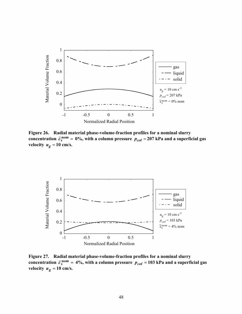
0
0.2
0.4
0.6
0.8
1
-1 -0.5 0 0.5 1
gasliquidsolid
Mat
eria
l Vol
ume
Frac
tion
Normalized Radial Position
ug = 10 cm s-1
pcol = 207 kPaεs = 0% nomnom
Figure 26. Radial material phase-volume-fraction profiles for a nominal slurry concentration =nom
sε 0%, with a column pressure =colp 207 kPa and a superficial gas velocity 10 cm/s. =gu
0
0.2
0.4
0.6
0.8
1
-1 -0.5 0 0.5 1
gasliquidsolid
Mat
eria
l Vol
ume
Frac
tion
Normalized Radial Position
ug = 10 cm s-1
pcol = 103 kPaεs = 4% nomnom
Figure 27. Radial material phase-volume-fraction profiles for a nominal slurry concentration =nom
sε 4%, with a column pressure =colp 103 kPa and a superficial gas velocity 10 cm/s. =gu
48

0
0.2
0.4
0.6
0.8
1
-1 -0.5 0 0.5 1
gasliquidsolid
Mat
eria
l Vol
ume
Frac
tion
Normalized Radial Position
ug = 10 cm s-1
pcol = 207 kPaεs = 4% nomnom
Figure 28. Radial material phase-volume-fraction profiles for a nominal slurry concentration =nom
sε 4%, with a column pressure =colp 207 kPa and a superficial gas velocity 10 cm/s. =gu
0
0.2
0.4
0.6
0.8
1
-1 -0.5 0 0.5 1
gasliquidsolid
Mat
eria
l Vol
ume
Frac
tion
Normalized Radial Position
ug = 10 cm s-1
pcol = 103 kPaεs = 8% nomnom
Figure 29. Radial material phase-volume-fraction profiles for a nominal slurry concentration =nom
sε 8%, with a column pressure =colp 103 kPa and a superficial gas velocity 10 cm/s. =gu
49
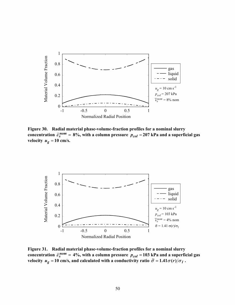
0
0.2
0.4
0.6
0.8
1
-1 -0.5 0 0.5 1
gasliquidsolid
Mat
eria
l Vol
ume
Frac
tion
Normalized Radial Position
ug = 10 cm s-1
pcol = 207 kPaεs = 8% nomnom
Figure 30. Radial material phase-volume-fraction profiles for a nominal slurry concentration =nom
sε 8%, with a column pressure =colp 207 kPa and a superficial gas velocity 10 cm/s. =gu
0
0.2
0.4
0.6
0.8
1
-1 -0.5 0 0.5 1
gasliquidsolid
Mat
eria
l Vol
ume
Frac
tion
Normalized Radial Position
ug = 10 cm s-1
pcol = 103 kPaεs = 4% nomσ = 1.41 σ(r)/σl
nom
~
Figure 31. Radial material phase-volume-fraction profiles for a nominal slurry concentration =nom
sε 4%, with a column pressure =colp 103 kPa and a superficial gas velocity 10 cm/s, and calculated with a conductivity ratio =gu lr σσσ )(41.1~ = .
50

0
0.2
0.4
0.6
0.8
1
-1 -0.5 0 0.5 1
gasliquidsolid
Mat
eria
l Vol
ume
Frac
tion
Normalized Radial Position
ug = 10 cm s-1
pcol = 207 kPaεs = 4% nomσ = 1.41 σ(r)/σl
nom
~
Figure 32. Radial material phase-volume-fraction profiles for a nominal slurry concentration =nom
sε 4%, with a column pressure =colp 207 kPa and a superficial gas velocity 10 cm/s, and calculated with a conductivity ratio =gu lr σσσ )(41.1~ = .
0
0.2
0.4
0.6
0.8
1
-1 -0.5 0 0.5 1
gasliquidsolid
Mat
eria
l Vol
ume
Frac
tion
Normalized Radial Position
ug = 10 cm s-1
pcol = 103 kPaεs = 8% nomσ = 0.94 σ(r)/σl
nom
~
Figure 33. Radial material phase-volume-fraction profiles for a nominal slurry concentration =nom
sε 8%, with a column pressure =colp 103 kPa and a superficial gas velocity 10 cm/s, and calculated with a conductivity ratio =gu lr σσσ )(94.0~ = .
51

0
0.2
0.4
0.6
0.8
1
-1 -0.5 0 0.5 1
gasliquidsolid
Mat
eria
l Vol
ume
Frac
tion
Normalized Radial Position
ug = 10 cm s-1
pcol = 207 kPaεs = 8% nomσ = 0.94 σ(r)/σl
nom
~
Figure 34. Radial material phase-volume-fraction profiles for a nominal slurry concentration =nom
sε 8%, with a column pressure =colp 207 kPa and a superficial gas velocity 10 cm/s, and calculated with a conductivity ratio =gu lr σσσ )(94.0~ = .
6. Conclusions and Future Recommendations This one-year LDRD project had two primary objectives: (1) to develop a new electrical-impedance tomography (EIT) diagnostic capable of quantitatively measuring material distributions of liquid-gas two-phase flows in industrially-relevant electrically-conducting vessels, specifically, in Sandia’s steel pilot-scale slurry bubble-column reactor (SBCR), and (2) to combine EIT with an established gamma-densitometry tomography (GDT) system to quantitatively measure material distributions of solid-liquid-gas three-phase flows in Sandia’s SBCR. An EIT diagnostic system was developed and applied to Sandia’s SBCR to measure two-phase-flow material distributions. These results for the bulk-averaged gas volume fractions were compared to the results obtained using an established GDT diagnostic system. The results had varying degrees of quantitative agreement with the GDT reference, ranging from a grouping of four tests with agreement to within 3.5% difference in magnitude, to a grouping of the remaining seven tests with agreement varying from 6.6% to 32.7%. There is no systematic explanation for these differences arising from variations in the prescribed flow conditions. A possible explanation for the range of agreements found in the results was provided. It was suggested that the invasiveness of the electrode rod used to apply the EIT system to the conducting vessel was creating a nonaxisymmetric flow-field disturbance that introduced a bias in the current flow paths between the current injection electrodes and ground. This nonaxisymmetric disturbance was not modeled in the FEM simulations used to reconstruct the electrical conductivity distributions and thus presented a source of possible significant error. Further characterization of
52

the degree of invasiveness of the electrode rod on the flow field is needed (e.g., using the GDT system to measure the phase volume fractions axially around the rod). Other means of positioning the electrode array throughout the flow domain (e.g., using an aerodynamically shaped rod or rake) to minimize the flow field disturbance should also be explored. It was believed that adding a nonconducting solid phase to the gas-liquid mixture in the column might reduce the bias in the current flow path described above and would therefore decrease the effect of the invasiveness of the rod on the flow field. In light of this, and in order to meet the second goal of this LDRD project, the EIT and GDT diagnostics were used in combination to make three-phase-flow material-distribution measurements in the SBCR. The results for the solid-phase fractions agreed well with the nominal solids loading fraction, after a correction was included to account for differences in the baseline liquid-only EIT measurements. Since the quantitative accuracy of the EIT system applied to metal vessels requires further examination, as shown from the two-phase-flow measurements, no conclusions are drawn as to the quantitative accuracy of the three-phase flow measurements. Two-phase and three-phase volumetric material distributions were measured using a newly designed EIT system in Sandia’s pilot-scale, industrially relevant SBCR. Although additional examination is required to assess the quantitative accuracy of the EIT measurements, qualitative trends were all as expected. This study demonstrates that EIT, after a little further development, can be a valuable diagnostic tool with potential to benefit a broad range of industries.
References Beck, M. S., Campogrande, E., Morris, M., Williams, R. A., and Waterfall, R. C., 1993,
Tomographic Techniques for Process Design and Operation, Computational Mechanics Publications, Southhampton, UK.
Boyer, C., Duquenne, A.-M., and Wild, G., 2002, "Measuring Techniques in Gas-Liquid and Gas-Liquid-Solid Reactors," Chemical Engineering Science, 57, 3185-3215.
Brown, B. H., 2001, "Medical Impedance Tomography and Process Impedance Tomography: a Brief Review," Measurement Science and Technology, 12, 991-996.
Ceccio, S. L., and George, D. L., 1996, "A Review of Electrical Impedance Techniques for the Measurement of Multiphase Flows," Journal of Fluids Engineering, 118, 391-399.
Chan, A. M., and Banerjee, S., 1981, "Design Aspects of Gamma Densitometers for Void Fraction Measurements in Small Scale Two-Phase Flows," Nuclear Instrumentation and Methods, 190, 135-148.
Chen, J., Li, F., Degaleesan, S., Gupta, P., Al-Dahhan, M. H., Dudukovic, M. P., and Toseland, B. A., 1999, "Fluid Dynamic Parameters in Bubble Columns with Internals," Chemical Engineering Science, 54, 2187-2197.
Deckwer, W.-D., 1992, Bubble Column Reactors, John Wiley and Sons, Chichester, England. Dudukovic, M. P., Larachi, F., and Mills, P. L., 1999, "Multiphase Reactors − Revisited,"
Chemical Engineering Science, 54, 1975-1995. Dyakowski, T., 1996, "Process Tomography Applied to Multi-Phase Flow Measurement,"
Measurement Science and Technology, 7, 343-353.
53

Fluent, I., 1998, FIDAP User's Manual, Version 8, Fluent, Inc., Lebanon, NH. George, D. L., Ceccio, S. L., O'Hern, T. J., Shollenberger, K. A., and Torczynski, J. R., 1998,
"Advanced Material Distribution Measurement in Multiphase Flows: A Case Study," ASME 1998 International Mechanical Engineering Congress and Exposition, Fluids Engineering Division, Anaheim, CA, FED-Vol. 247, 31-42.
George, D. L., Ceccio, S. L., Torczynski, J. R., Shollenberger, K. A., and O'Hern, T. J., 1999, "Quantitative Phase Distribution Measurements in Three-Phase Flows," ASME/JSME Joint Fluids Engineering Conference, San Francisco, CA, FEDSM99-7375.
George, D. L., Shollenberger, K. A., and Torczynski, J. R., 2000a, "Sparger Effects on Gas Volume Fraction Distributions in Vertical Bubble-Column Flows as Measured by Gamma-Densitometry Tomography," ASME 2000 Fluids Engineering Division Summer Meeting, Boston, MA, FEDSM2000-1132.
George, D. L., Shollenberger, K. A., Torczynski, J. R., O'Hern, T. J., and Ceccio, S. L., 2001a, "Three-Phase Material Distribution Measurement in a Vertical Flow Using Gamma-Densitometry Tomography and Electrical-Impedance Tomography," International Journal of Multiphase Flow, 27(1903-1930).
George, D. L., Torczynski, J. R., O'Hern, T. J., Shollenberger, K. A., Tortora, P. R., and Ceccio, S. L., 2000b, "Quantitative Electrical-Impedance Tomography in an Electrically Conducting Bubble-Column Vessel," ASME 2001 Fluids Engineering Division Summer Meeting, New Orleans, LA, FEDSM2001-18031.
George, D. L., Torczynski, J. R., O'Hern, T. J., Shollenberger, K. A., Tortora, P. R., and Ceccio, S. L., 2001b, "Quantitative Electrical-Impedance Tomography in an Electrically Conducting Bubble-Column Vessel," ASME 2001 Fluids Engineering Division Summer Meeting, New Orleans, LA, FEDSM2001-18031.
George, D. L., Torczynski, J. R., Shollenberger, K. A., O'Hern, T. J., and Ceccio, S. L., 2000c, "Quantitative Tomographic Measurements of Opaque Multiphase Flows," Sandia Report No. SAND2000-0443, Sandia National Laboratories, Albuquerque, NM.
George, D. L., Torczynski, J. R., Shollenberger, K. A., O'Hern, T. J., and Ceccio, S. L., 2000d, "Validation of Electrical-Impedance Tomography for Measurements of Material Distribution in Two-Phase Flows," International Journal of Multiphase Flow, 26, 549-581.
Hewitt, G. F., 1978, Measurement of Two-Phase Flow Parameters, Academic Press, London. Jackson, N. B., Torczynski, J. R., Shollenberger, K. A., O'Hern, T. J., and Adkins, D. R., 1996,
"Hydrodynamic Characterization of Slurry Bubble-Column Reactors for Fischer-Tropsch Synthesis," Proceedings of the Thirteenth Annual International Pittsburgh Coal Conference, Vol. 2: Coal-Energy and the Environment, S.-H. Chiang, ed., University of Pittsburgh Center for Energy Research, Pittsburgh, PA, 299-325.
Lapp, R. E., and Andrews, H. L., 1972, Nuclear Radiation Physics, Prentice-Hall, Englewood Cliffs, NJ.
Lemonnier, H., 1997, "Multiphase Instrumentation: The Keystone of Multidimensional Multiphase Flow Modeling," Experimental Thermal and Fluid Science, 15, 154-162.
Liter, S. G., Shollenberger, K. A., Torczynski, J. R., and Ceccio, S. L., 2002, "Measuring Material Distributions of Multiphase Flows in Electrically Conducting Vessels Using Electrical-Impedance Tomography," ASME 2002 Fluids Engineering Division Summer Meeting, Montreal, Quebec, Canada, FEDSM2002-31377.
Maxwell, J. C., 1881, A Treatise on Electricity and Magnetism, Oxford University Press, Oxford.
54

Petrick, M., and Swanson, B. S., 1958, "Radiation Attenuation Method of Measuring Density of a Two-Phase Flow," Review of Scientific Instruments, 29, 1079-1085.
Shah, Y. T., and Deckwer, W.-D., 1983, "Hydrodynamics of Bubble Columns," Handbook of Fluids in Motion, R. Gupta, ed., Ann Arbor Science, Ann Arbor, MI.
Shollenberger, K. A., George, D. L., and Torczynski, J. R., 2000, "Effect of Sparger Geometry on Gas-Volume-Fraction in Bubble-Column Flows Measured by Gamma-Densitometry Tomography (GDT)," AIChE 2000 Annual Meeting, Los Angeles, CA, Paper No. 344c.
Shollenberger, K. A., Torczynski, J. R., Adkins, D. R., and O'Hern, T. J., 1995, "Bubble Column Measurements Using Gamma Tomography," The 1995 ASME/JSME Fluids Engineering and Laser Anemometry Conference and Exhibition, Hilton Head, SC, FED-Vol. 211, 25-30.
Shollenberger, K. A., Torczynski, J. R., Adkins, D. R., O'Hern, T. J., and Jackson, N. B., 1997a, "Gamma-Densitometry Tomography of Gas Holdup Spatial Distribution in Industrial-Scale Bubble Columns," Chemical Engineering Science, 52(13), 2037-2048.
Shollenberger, K. A., Torczynski, J. R., and George, D. L., 2002, "Gas Distribution in Air/Water and Air/Oil Bubble-Column Flows," ASME 2002 Fluids Engineering Division Summer Meeting, Montreal, Quebec, Canada, FEDSM2002-31376.
Shollenberger, K. A., Torczynski, J. R., O'Hern, T. J., Adkins, D. R., Ceccio, S. L., and George, D. L., 1997b, "Comparison of Gamma-Densitometry Tomography and Electrical-Impedance Tomography for Determining Material Distribution in Liquid-Solid Flows," ASME 1997 Fluids Engineering Division Summer Meeting, Vancouver, British Columbia, Canada, FEDSM97-3690.
Swift, W. L., Dolan, R. X., and Runstadler, P. W., 1978, "A Scanning Gamma Ray Attenuation System for Void Fraction Measurements in Two-Phase Flows," ASME Proceedings, Measurements in Polyphase Flows, D. Stock, ed., 25-35.
Torczynski, J. R., Adkins, D. R., Shollenberger, K. A., and O'Hern, T. J., 1996, "Application of Gamma-Densitometry Tomography to Determine Phase Spatial Variation in Two-Phase and Three-Phase Bubble Flows," ASME 1996 Fluids Engineering Division Summer Meeting, San Diego, CA, FED-Vol. 236, 503-508.
Torczynski, J. R., O'Hern, T. J., Adkins, D. R., Jackson, N. B., and Shollenberger, K. A., 1997, "Advanced Tomographic Flow Diagnostics for Opaque Multiphase Fluids," Sandia Report No. SAND97-1176, Sandia National Laboratories, Albuquerque, NM.
Vest, C. M., 1985, "Tomography for Properties of Materials that Bend Rays: A Tutorial," Applied Optics, 24(23), 4089-4094.
Wang, M., Dorward, A., Vlaev, D., and Mann, R., 2000, "Measurements of Gas-Liquid Mixing in a Stirred Vessel Using Electrical Resistance Tomography (ERT)," Chemical Engineering Journal, 77, 93-98.
Williams, R. A., and Beck, M. S., 1995, Process Tomography: Principles, Techniques, and Applications, Butterworth-Heinemann, Oxford, England.
York, T., 2001, "Status of Electrical Tomography in Industrial Applications," Journal of Electronic Imaging, 10(3), 608-619.
Yuen, E. L., Mann, R., York, T. A., and Grieve, B. D., 2001, "Electrical Resistance Tomography (ERT) Imaging of a Metal-Walled Solid-Liquid Filter," 2nd World Congress on Industrial Process Tomography, Hanover, Germany, 183-190.
55

Appendix The following FORTRAN77 numerical codes were used in this study to compute the phase-material distributions from the EIT voltage and GDT line-averaged intensity measurements. The following program was used to reconstruct the parabolic radial normalized conductivity distribution from the EIT voltage and current measurements. c c2345678901234567890123456789012345678901234567890123456789012345678901 c program eittab c implicit double precision (a-h,o-z) c c added line 109,110,111 c 113-114 c 115-116 c changed 261 c added 262-263 c changed 470 c added 471-472 c 535-545 c modified as above by SGL 09/18/02 c written by JRT c c *** 020405 c c *** This program searches a table of precomputed voltages c to find the closest match to experimental voltages. c If the match is not on the table boundary, c interpolation is performed to improve the match. c c *** Files used. c c eittab_inp.dat (input) c 1 line: 0/1, use/ignore injection electrode voltage c 1 line: 0/1, use/ignore ground electrode voltage c 1 line: 0/1, use/ignore voltages when injection = ground c 1 line: 0/1/2, no offset/ground offset/injection-ground offset c 1 line: 0/1, use/ignore measured current c 1 line: 0/1, interpolate/don't interpolate c 1 line: 0/1, write to screen/don't write to screen c c eittab_cmp.dat (input) c 1 line: ntb, number of computed table entries c 1 line: ncp, number of nontrivial conductivity parameters c ncp lines: cmin(i), cmax(i), cinc(i), i=1,ncp,1 c 1 line: min and max injection electrode number c 1 line: min and max ground electrode number
56
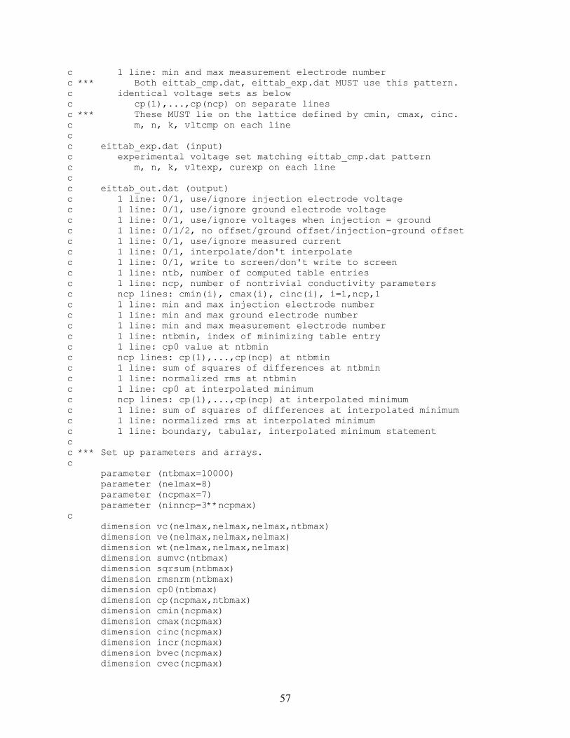
c 1 line: min and max measurement electrode number c *** Both eittab_cmp.dat, eittab_exp.dat MUST use this pattern. c identical voltage sets as below c cp(1),...,cp(ncp) on separate lines c *** These MUST lie on the lattice defined by cmin, cmax, cinc. c m, n, k, vltcmp on each line c c eittab_exp.dat (input) c experimental voltage set matching eittab_cmp.dat pattern c m, n, k, vltexp, curexp on each line c c eittab_out.dat (output) c 1 line: 0/1, use/ignore injection electrode voltage c 1 line: 0/1, use/ignore ground electrode voltage c 1 line: 0/1, use/ignore voltages when injection = ground c 1 line: 0/1/2, no offset/ground offset/injection-ground offset c 1 line: 0/1, use/ignore measured current c 1 line: 0/1, interpolate/don't interpolate c 1 line: 0/1, write to screen/don't write to screen c 1 line: ntb, number of computed table entries c 1 line: ncp, number of nontrivial conductivity parameters c ncp lines: cmin(i), cmax(i), cinc(i), i=1,ncp,1 c 1 line: min and max injection electrode number c 1 line: min and max ground electrode number c 1 line: min and max measurement electrode number c 1 line: ntbmin, index of minimizing table entry c 1 line: cp0 value at ntbmin c ncp lines: cp(1),...,cp(ncp) at ntbmin c 1 line: sum of squares of differences at ntbmin c 1 line: normalized rms at ntbmin c 1 line: cp0 at interpolated minimum c ncp lines: cp(1),...,cp(ncp) at interpolated minimum c 1 line: sum of squares of differences at interpolated minimum c 1 line: normalized rms at interpolated minimum c 1 line: boundary, tabular, interpolated minimum statement c c *** Set up parameters and arrays. c parameter (ntbmax=10000) parameter (nelmax=8) parameter (ncpmax=7) parameter (ninncp=3**ncpmax) c dimension vc(nelmax,nelmax,nelmax,ntbmax) dimension ve(nelmax,nelmax,nelmax) dimension wt(nelmax,nelmax,nelmax) dimension sumvc(ntbmax) dimension sqrsum(ntbmax) dimension rmsnrm(ntbmax) dimension cp0(ntbmax) dimension cp(ncpmax,ntbmax) dimension cmin(ncpmax) dimension cmax(ncpmax) dimension cinc(ncpmax) dimension incr(ncpmax) dimension bvec(ncpmax) dimension cvec(ncpmax)
57

dimension dvec(ncpmax) dimension amat(ncpmax,ncpmax) dimension cmat(ncpmax,ncpmax) dimension dmat(ncpmax,ncpmax) dimension cint(ncpmax) dimension vvvv(ncpmax) dimension map(ninncp) dimension sq(ninncp) dimension c0(ninncp) character*4 fdc character*2 fdn character*1 contynrn, contynfc c 0001 write(6,*)'input flow condition ####' read *, fdc 0002 write(6,*)'input flow run number ##' read *, fdn c c *** Formats. c 1001 format(i2) 1002 format(i8) 1003 format(2(1x,i2)) 1004 format(3(1x,d12.6)) 1005 format(i8,3(1x,d12.6)) 2001 format(a) c c *** Initialize all quantities to zero. c do 0020 i9 = 1, ntbmax, 1 sumvc(i9) = 0. sqrsum(i9) = 0. rmsnrm(i9) = 0. cp0(i9) = 0. do 0010 i4 = 1, ncpmax, 1 cp(i4,i9) = 0. 0010 continue 0020 continue c do 0040 i3 = 1, nelmax, 1 do 0040 i2 = 1, nelmax, 1 do 0040 i1 = 1, nelmax, 1 wt(i1,i2,i3) = 0. ve(i1,i2,i3) = 0. do 0030 i9 = 1, ntbmax, 1 vc(i1,i2,i3,i9) = 0. 0030 continue 0040 continue c do 0060 i4 = 1, ncpmax, 1 cmin(i4) = 0. cmax(i4) = 0. cinc(i4) = 0. incr(i4) = 0. bvec(i4) = 0. cvec(i4) = 0. dvec(i4) = 0.
58

cint(i4) = 0. vvvv(i4) = 0. do 0050 i5 = 1, ncpmax, 1 amat(i4,i5) = 0. cmat(i4,i5) = 0. dmat(i4,i5) = 0. 0050 continue 0060 continue c do 0070 i6 = 1, ninncp, 1 map(i6) = 0 sq(i6) = 0. c0(i6) = 0. 0070 continue c c *** Read in processing options. c open (unit=21,status='old',file='eittab_inp.dat') c read (21,*) noinjc read (21,*) nogrnd read (21,*) noingr read (21,*) nooffs read (21,*) nocurr read (21,*) nointe read (21,*) noscre c close (unit=21) c c *** Read in computed tabular voltages. c open (unit=22,status='old',file='eittab_cmp.dat') c read (22,*) ntb if ((ntb.lt.1).or.(ntb.gt.ntbmax)) then write (6,*) 'Requested table entries: ', ntb write (6,*) 'Allowed table entries: ', 1, ntbmax write (6,*) 'Recompile with larger ntbmax.' close (unit=22) go to 9999 end if c read (22,*) ncp if ((ncp.lt.0).or.(ncp.gt.ncpmax)) then write (6,*) 'Requested cond. params.: ', ncp write (6,*) 'Allowed cond. params.: ', 0, ncpmax write (6,*) 'Recompile with larger ncpmax.' close (unit=22) go to 9999 end if c do 0100 i4 = 1, ncp, 1 read (22,*) cmin(i4), cmax(i4), cinc(i4) 0100 continue c read (22,*) ninjc1, ninjc2 read (22,*) ngrnd1, ngrnd2
59

read (22,*) nmeas1, nmeas2 if ((ninjc1.gt.ninjc2).or.(ngrnd1.gt.ngrnd2).or. 1 (nmeas1.gt.nmeas2)) then write (6,*) 'Requested electrode bounds misordered:' write (6,*) ninjc1, ninjc2 write (6,*) ngrnd1, ngrnd2 write (6,*) nmeas1, nmeas2 close (unit=22) go to 9999 end if minel=min(ninjc1,min(ngrnd1,nmeas1)) maxel=max(ninjc2,max(ngrnd2,nmeas2)) if ((minel.lt.1).or.(maxel.gt.nelmax)) then write (6,*) 'Requested electrode bounds: ', minel, maxel write (6,*) 'Allowed electrode bounds: ', 1, nelmax close (unit=22) go to 9999 end if c do 0130 i9 = 1, ntb, 1 do 0110 i4 = 1, ncp, 1 read (22,*) cp(i4,i9) if ((cp(i4,i9).lt.cmin(i4)).or.(cp(i4,i9).gt.cmax(i4))) then write (6,*) 'Requested param.: ', i4, i9, cp(i4,i9) write (6,*) 'Allowed param.: ', cmin(i4), cmax(i4) close (unit=22) go to 9999 end if 0110 continue do 0120 mm = ninjc1, ninjc2, 1 do 0120 nn = ngrnd1, ngrnd2, 1 do 0120 kk = nmeas1, nmeas2, 1 read (22,*) m, n, k, vltcmp if ((m.ne.mm).or.(n.ne.nn).or.(k.ne.kk)) then write (6,*) 'Requested electrodes: ', m, n, k write (6,*) 'Expected electrodes: ', mm, nn, kk close (unit=22) go to 9999 end if vc(mm,nn,kk,i9) = vltcmp 0120 continue 0130 continue c close (unit=22) c c *** Read in experimental voltages and currents. c c open (unit=23,status='old',file='eittab_exp.dat') open (unit=23,status='old',file='../../data/e/3Peit/G2' 1//fdc//'/mo/G2'//fdc//fdn//'.dat') c do 0140 mm = ninjc1, ninjc2, 1 do 0140 nn = ngrnd1, ngrnd2, 1 do 0140 kk = nmeas1, nmeas2, 1 read (23,*) m, n, k, vltexp, curexp if ((m.ne.mm).or.(n.ne.nn).or.(k.ne.kk)) then write (6,*) 'Requested electrodes: ', m, n, k
60
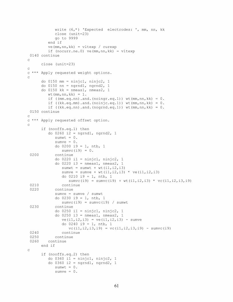
write (6,*) 'Expected electrodes: ', mm, nn, kk close (unit=23) go to 9999 end if ve(mm,nn,kk) = vltexp / curexp if (nocurr.ne.0) ve(mm,nn,kk) = vltexp 0140 continue c close (unit=23) c c *** Apply requested weight options. c do 0150 mm = ninjc1, ninjc2, 1 do 0150 nn = ngrnd1, ngrnd2, 1 do 0150 kk = nmeas1, nmeas2, 1 wt(mm,nn,kk) = 1. if ((mm.eq.nn).and.(noingr.eq.1)) wt(mm,nn,kk) = 0. if ((kk.eq.mm).and.(noinjc.eq.1)) wt(mm,nn,kk) = 0. if ((kk.eq.nn).and.(nogrnd.eq.1)) wt(mm,nn,kk) = 0. 0150 continue c c *** Apply requested offset option. c if (nooffs.eq.1) then do 0260 i2 = ngrnd1, ngrnd2, 1 sumwt = 0. sumve = 0. do 0200 i9 = 1, ntb, 1 sumvc(i9) = 0. 0200 continue do 0220 i1 = ninjc1, ninjc2, 1 do 0220 i3 = nmeas1, nmeas2, 1 sumwt = sumwt + wt(i1,i2,i3) sumve = sumve + wt(i1,i2,i3) * ve(i1,i2,i3) do 0210 i9 = 1, ntb, 1 sumvc(i9) = sumvc(i9) + wt(i1,i2,i3) * vc(i1,i2,i3,i9) 0210 continue 0220 continue sumve = sumve / sumwt do 0230 i9 = 1, ntb, 1 sumvc(i9) = sumvc(i9) / sumwt 0230 continue do 0250 i1 = ninjc1, ninjc2, 1 do 0250 i3 = nmeas1, nmeas2, 1 ve(i1,i2,i3) = ve(i1,i2,i3) - sumve do 0240 i9 = 1, ntb, 1 vc(i1,i2,i3,i9) = vc(i1,i2,i3,i9) - sumvc(i9) 0240 continue 0250 continue 0260 continue end if c if (nooffs.eq.2) then do 0360 i1 = ninjc1, ninjc2, 1 do 0360 i2 = ngrnd1, ngrnd2, 1 sumwt = 0. sumve = 0.
61

do 0300 i9 = 1, ntb, 1 sumvc(i9) = 0. 0300 continue do 0320 i3 = nmeas1, nmeas2, 1 sumwt = sumwt + wt(i1,i2,i3) sumve = sumve + wt(i1,i2,i3) * ve(i1,i2,i3) do 0310 i9 = 1, ntb, 1 sumvc(i9) = sumvc(i9) + wt(i1,i2,i3) * vc(i1,i2,i3,i9) 0310 continue 0320 continue sumve = sumve / sumwt do 0330 i9 = 1, ntb, 1 sumvc(i9) = sumvc(i9) / sumwt 0330 continue do 0350 i3 = nmeas1, nmeas2, 1 ve(i1,i2,i3) = ve(i1,i2,i3) - sumve do 0340 i9 = 1, ntb, 1 vc(i1,i2,i3,i9) = vc(i1,i2,i3,i9) - sumvc(i9) 0340 continue 0350 continue 0360 continue end if c c *** Find minimizing table entry. c ntbmin = 1 sum1 = 0. do 0420 i1 = ninjc1, ninjc2, 1 do 0420 i2 = ngrnd1, ngrnd2, 1 do 0420 i3 = nmeas1, nmeas2, 1 sum1 = sum1 + wt(i1,i2,i3) * ve(i1,i2,i3) ** 2 0420 continue do 0490 i9 = 1, ntb, 1 sum2 = 0. sum3 = 0. do 0450 i1 = ninjc1, ninjc2, 1 do 0450 i2 = ngrnd1, ngrnd2, 1 do 0450 i3 = nmeas1, nmeas2, 1 sum2 = sum2 + wt(i1,i2,i3) * ve(i1,i2,i3) * vc(i1,i2,i3,i9) sum3 = sum3 + wt(i1,i2,i3) * vc(i1,i2,i3,i9) ** 2 0450 continue cp0(i9) = sum2 / sum3 sqrsum(i9) = sum1 - 2.*sum2*cp0(i9) + sum3*cp0(i9)**2 rmsnrm(i9) = sqrt(abs(sqrsum(i9))/sum1) if (sqrsum(i9).lt.sqrsum(ntbmin)) ntbmin = i9 0490 continue c c *** Interpolate off table if requested. c *** Do nothing if minimizing table entry on boundary. c if (nointe.eq.0) then c do 0520 i9 = 1, ntb, 1 inside = 1 do 0510 i4 = 1, ncp, 1 incr(i4) = 1 + nint((cp(i4,i9)-cp(i4,ntbmin))/cinc(i4)) if ((incr(i4).lt.0).or.(incr(i4).gt.2)) inside = 0
62

0510 continue if (inside.eq.1) then call inline(ncp,incr,i8) map(i8) = i9 sq(i8) = sqrsum(i9) c0(i8) = cp0(i9) end if 0520 continue c ifull = 1 do 0530 i8 = 1, 3**ncp, 1 if (map(i8).lt.1) ifull = 0 0530 continue c if (ifull.eq.1) then c do 0550 i4 = 1, ncp, 1 do 0540 i6 = 1, ncp, 1 incr(i6) = 1 0540 continue incr(i4) = 0 call inline(ncp,incr,i80) incr(i4) = 1 call inline(ncp,incr,i81) incr(i4) = 2 call inline(ncp,incr,i82) cvec(i4) = 0.5 * ( c0(i80) - c0(i82) ) cmat(i4,i4) = c0(i80) - 2. * c0(i81) + c0(i82) bvec(i4) = 0.5 * ( sq(i80) - sq(i82) ) amat(i4,i4) = sq(i80) - 2. * sq(i81) + sq(i82) dvec(i4) = bvec(i4) dmat(i4,i4) = amat(i4,i4) 0550 continue c do 0570 i5 = 1, ncp, 1 do 0570 i4 = 1, ncp, 1 if (i4.ne.i5) then do 0560 i6 = 1, ncp, 1 incr(i6) = 1 0560 continue incr(i4) = 0 incr(i5) = 0 call inline(ncp,incr,i800) incr(i4) = 0 incr(i5) = 2 call inline(ncp,incr,i802) incr(i4) = 2 incr(i5) = 0 call inline(ncp,incr,i820) incr(i4) = 2 incr(i5) = 2 call inline(ncp,incr,i822) cmat(i4,i5) = 0.25 * ( c0(i800) - c0(i802) 1 - c0(i820) + c0(i822) ) amat(i4,i5) = 0.25 * ( sq(i800) - sq(i802) 1 - sq(i820) + sq(i822) ) dmat(i4,i5) = amat(i4,i5)
63

end if 0570 continue c call ludcmp(dmat,ncp,ncpmax,incr,dpar,vvvv) call lubksb(dmat,ncp,ncpmax,incr,dvec) c sqint = sqrsum(ntbmin) cint0 = cp0(ntbmin) do 0590 i4 = 1, ncp, 1 cint(i4) = cp(i4,ntbmin) + cinc(i4) * dvec(i4) sqint = sqint - bvec(i4) * dvec(i4) cint0 = cint0 - cvec(i4) * dvec(i4) do 0580 i5 = 1, ncp, 1 sqint = sqint + 0.5 * dvec(i4) * amat(i4,i5) * dvec(i5) cint0 = cint0 + 0.5 * dvec(i4) * cmat(i4,i5) * dvec(i5) 0580 continue 0590 continue noexac = 0 if (sqint.lt.0.) noexac = 1 rmsint = sqrt(abs(sqint)/sum1) c end if c end if c c *** Write results out to file. c c open (unit=24,status='unknown',file='eittab_out.dat') open (unit=24,status='unknown',file='../../data/e/3Peit/G2' 1//fdc//'/res/G2'//fdc//fdn//'eittabr.dat') c nout1 = 6 nout2 = 24 nout0 = nout2 - nout1 if (noscre.ne.0) nout1 = nout2 c do 0930 nout = nout1, nout2, nout0 c write (nout,1001) noinjc write (nout,1001) nogrnd write (nout,1001) noingr write (nout,1001) nooffs write (nout,1001) nocurr write (nout,1001) nointe write (nout,1001) noscre c write (nout,1002) ntb write (nout,1002) ncp do 0900 i4 = 1, ncp, 1 write (nout,1004) cmin(i4), cmax(i4), cinc(i4) 0900 continue write (nout,1003) ninjc1, ninjc2 write (nout,1003) ngrnd1, ngrnd2 write (nout,1003) nmeas1, nmeas2 c write (nout,2001) 'Tabular minimum: ' write (nout,1002) ntbmin
64

write (nout,1004) cp0(ntbmin) do 0910 i4 = 1, ncp, 1 write (nout,1004) cp(i4,ntbmin) 0910 continue write (nout,1004) sqrsum(ntbmin) write (nout,1004) rmsnrm(ntbmin) c if (nointe.eq.0) then if (ifull.eq.1) then if (noexac.eq.0) then write (nout,2001) 'Interpolated minimum acceptable: ' else write (nout,2001) 'Interpolated minimum questionable: ' end if write (nout,1004) cint0 do 0920 i4 = 1, ncp, 1 write (nout,1004) cint(i4) 0920 continue write (nout,1004) sqint write (nout,1004) rmsint else write (nout,2001) 'No interpolation although requested: ' write (nout,2001) 'Tabular minimum lies on boundary' end if else write (nout,2001) 'No interpolation requested' end if c 0930 continue c close (unit=24) c c *** Stop, end. c 9999 continue write (6,*) 'Continue with new run number? (y,n)' read *, contynrn if (contynrn.eq.'y') then goto 0002 endif write (6,*) 'Continue with new flow condition? (y,n)' read *, contynfc if (contynfc.eq.'y') then goto 0001 endif c stop 'eittab' end c c23456789012345678901234567890123456789012345678901234567890123456789012 c subroutine inline(ncp,incr,i8) c implicit double precision (a-h,o-z) c dimension incr(ncp) c
65
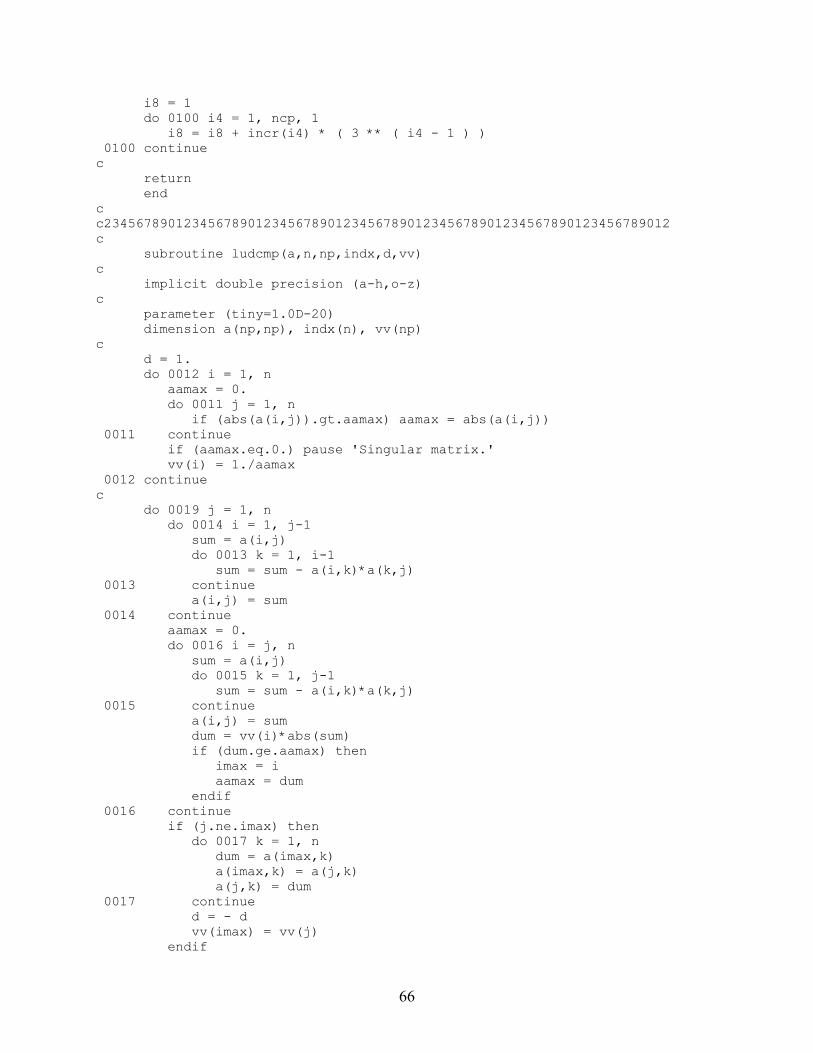
i8 = 1 do 0100 i4 = 1, ncp, 1 i8 = i8 + incr(i4) * ( 3 ** ( i4 - 1 ) ) 0100 continue c return end c c23456789012345678901234567890123456789012345678901234567890123456789012 c subroutine ludcmp(a,n,np,indx,d,vv) c implicit double precision (a-h,o-z) c parameter (tiny=1.0D-20) dimension a(np,np), indx(n), vv(np) c d = 1. do 0012 i = 1, n aamax = 0. do 0011 j = 1, n if (abs(a(i,j)).gt.aamax) aamax = abs(a(i,j)) 0011 continue if (aamax.eq.0.) pause 'Singular matrix.' vv(i) = 1./aamax 0012 continue c do 0019 j = 1, n do 0014 i = 1, j-1 sum = a(i,j) do 0013 k = 1, i-1 sum = sum - a(i,k)*a(k,j) 0013 continue a(i,j) = sum 0014 continue aamax = 0. do 0016 i = j, n sum = a(i,j) do 0015 k = 1, j-1 sum = sum - a(i,k)*a(k,j) 0015 continue a(i,j) = sum dum = vv(i)*abs(sum) if (dum.ge.aamax) then imax = i aamax = dum endif 0016 continue if (j.ne.imax) then do 0017 k = 1, n dum = a(imax,k) a(imax,k) = a(j,k) a(j,k) = dum 0017 continue d = - d vv(imax) = vv(j) endif
66

indx(j) = imax if (a(j,j).eq.0.) then a(j,j) = tiny write (6,*) 'Using tiny:', tiny endif if (j.ne.n) then dum = 1./a(j,j) do 0018 i = j+1, n a(i,j) = a(i,j) * dum 0018 continue endif 0019 continue c return end c c23456789012345678901234567890123456789012345678901234567890123456789012 c subroutine lubksb(a,n,np,indx,b) c implicit double precision (a-h,o-z) c dimension a(np,np), indx(n), b(n) c ii = 0 do 0012 i = 1, n ll = indx(i) sum = b(ll) b(ll) = b(i) if (ii.ne.0) then do 0011 j = ii, i-1 sum = sum - a(i,j)*b(j) 0011 continue else if (sum.ne.0.) then ii = i endif b(i) = sum 0012 continue c do 0014 i = n, 1, -1 sum = b(i) if (i.lt.n) then do 0013 j = i+1, n sum = sum - a(i,j)*b(j) 0013 continue endif b(i) = sum / a(i,i) 0014 continue c return end c c23456789012345678901234567890123456789012345678901234567890123456789012 c
67

The following program was used to reconstruct the parabolic radial normalized attenuation coefficient distribution from the linq-averaged, GDT intensity measurements. c c23456789012345678901234567890123456789012345678901234567890123456789012 c program gdtaxi c c Revision 5/30/99 by dlg c c *** Gamma-densitometry tomography axisymmetric reconstruction c using even radial polynomials. c implicit double precision (a-h,o-z) c parameter (nsm=1000) parameter (nfcnm=10) dimension spos(nsm), full(nsm), empt(nsm), flow(nsm) dimension snrm(nsm), void(nsm) dimension nexp(nfcnm), amat(nfcnm,nfcnm), bvec(nfcnm) dimension cmat(nfcnm,nfcnm) dimension ravf(nsm), axvf(nsm) dimension cravf(nfcnm), caxvf(nfcnm) dimension cramf(nfcnm), caxmf(nfcnm) dimension ccoeff(nfcnm,nfcnm), dcoeff(nfcnm,nfcnm) character*6 fname c 1001 format (1x,f11.5) 1002 format (1x,i11) 1003 format (1x,i11,5(1x,f11.5)) 1004 format (6(1x,f11.5)) 2000 format (1x,a) 2001 format (1x,a11,f11.5) 2002 format (1x,a11,i11) c c *** Read in geometric and fitting information. c write (6,2000) 'Reading input parameters from gdtaxi_inp.dat' open (unit=24, status='old', file='gdtaxi_inp.dat') read (24,*) fname read (24,*) rinner read (24,*) scentr read (24,*) dxedge read (24,*) iclip read (24,*) cliplo read (24,*) cliphi read (24,*) tau read (24,*) nexpm write (6,*) ' fname = ', fname write (6,2001) ' rinner = ', rinner write (6,2001) ' scentr = ', scentr write (6,2001) ' dxedge = ', dxedge write (6,2002) ' iclip = ', iclip write (6,2001) ' cliplo = ', cliplo write (6,2001) ' cliphi = ', cliphi write (6,2001) ' tau = ', tau
68

write (6,2002) ' nexpm = ', nexpm close (unit=24) c c *** Echo information to output file. c write (6,2000) 'Writing input parameters to gdtaxi_out.dat' open (unit=30, status='unknown', file=fname//'_out.dat') write (30,1001) rinner write (30,1001) scentr write (30,1001) dxedge write (30,1002) iclip write (30,1001) cliplo write (30,1001) cliphi write (30,1001) tau write (30,1002) nexpm c c *** Read in full, empty, flow scans. c *** Do some error checking for consistent files. c write (6,2000) 'Reading experimental data from ' write (6,2000) ' gdtaxi_ful.dat gdtaxi_emp.dat '//fname//'.DAT' open (unit=21, status='old', file='gdtaxi_ful.dat') open (unit=22, status='old', file='gdtaxi_emp.dat') open (unit=23, status='old', file=fname//'.DAT') read (21,*) x1f, dxf, xnf, y1f, dyf, ynf read (22,*) x1e, dxe, xne, y1e, dye, yne read (23,*) x1b, dxb, xnb, y1b, dyb, ynb nxf = nint(xnf) nyf = nint(ynf) nxe = nint(xne) nye = nint(yne) nxb = nint(xnb) nyb = nint(ynb) if ((nyf.ne.nye).or.(nyf.ne.nyb)) then write (6,*) '*** VERT. SCANS HAVE DIFFERENT # OF POINTS ***' write (6,*) 'ful ', nyf, ' emp ', nye, ' flo ', nyb go to 998 end if tol = 0.05 * rinner if ((abs(y1f-y1e).gt.tol).or.(abs(y1f-y1b).gt.tol)) then write (6,*) '*** VERT. SCANS HAVE DIFFERENT ORIGINS ***' write (6,*) 'ful ', y1f, ' emp ', y1e, ' flo ', y1b go to 998 end if if ((abs(dyf-dye).gt.tol).or.(abs(dyf-dyb).gt.tol)) then write (6,*) '*** VERT. SCANS HAVE DIFFERENT STEP SIZES ***' write (6,*) 'ful ', dyf, ' emp ', dye, ' flo ', dyb go to 998 end if if ((nxf.ne.nxe).or.(nxf.ne.nxb)) then write (6,*) '*** HORIZ. SCANS HAVE DIFFERENT # OF POINTS ***' write (6,*) 'ful ', nxf, ' emp ', nxe, ' flo ', nxb go to 998 end if if ((abs(x1f-x1e).gt.tol).or.(abs(x1f-x1b).gt.tol)) then write (6,*) '*** HORIZ. SCANS HAVE DIFFERENT ORIGINS ***' write (6,*) 'ful ', x1f, ' emp ', x1e, ' flo ', x1b
69

go to 998 end if if ((abs(dxf-dxe).gt.tol).or.(abs(dxf-dxb).gt.tol)) then write (6,*) '*** HORIZ. SCANS HAVE DIFF. STEP SIZES ***' write (6,*) 'ful ', dxf, ' emp ', dxe, ' flo ', dxb go to 998 end if if (nxf+1.gt.nsm) then write (6,*) '*** NOT ENOUGH POINTS AVAILABLE ***' write (6,*) nxf, nsm go to 998 end if c c *** Skip header information c read (21,*) tmlive read (22,*) tmlive read (23,*) tmlive c c *** Open output files. c open (unit=28, status='unknown', file=fname//'_gas.dat') open (unit=29, status='unknown', file=fname//'_liq.dat') c c *** Read in data and compute the nominal rates. c nt = nyf + 1 do 460 js = 1, nt, 1 ns = nxf + 1 do 100 is = 1, ns, 1 read (21,*,end=998,err=998) sposx, sposy, frate read (22,*,end=998,err=998) sposx, sposy, erate read (23,*,end=998,err=998) sposx, sposy, brate spos(is) = sposx full(is) = frate empt(is) = erate flow(is) = brate 100 continue c c *** Compute best fit to ray averages. c write (6,2000) 'Computing results' nfcn = nexpm / 2 + 1 if (nfcn.gt.nfcnm) then write (6,2000) '*** NOT ENOUGH FITTING FUNC. AVAILABLE ***' write (6,2000) nfcn, nfcnm go to 998 end if do 120 ifcn = 1, nfcn, 1 nexp(ifcn) = 2 * ( ifcn - 1 ) 120 continue c c *** Correct the rates for nonlinear detector response. c do 140 is = 1, ns, 1 full(is) = full(is) / ( 1. - full(is) * tau ) empt(is) = empt(is) / ( 1. - empt(is) * tau )
70

flow(is) = flow(is) / ( 1. - flow(is) * tau ) 140 continue c c *** Take logarithms to get absorptions. c do 150 is = 1, ns, 1 full(is) = - log( full(is) ) empt(is) = - log( empt(is) ) flow(is) = - log( flow(is) ) 150 continue c c *** Compute left and right array bounds for inner diameter. c s1 = scentr - rinner + dxedge s2 = scentr + rinner - dxedge ns1 = 1 ns2 = 0 do 160 is = 1, ns, 1 if (spos(is).le.s1) ns1 = ns1 + 1 if (spos(is).lt.s2) ns2 = ns2 + 1 160 continue c c *** Compute the norm. position and the avg. void fraction on rays. c do 180 is = 1, ns, 1 snrm(is) = ( spos(is) - scentr ) / rinner void(is) = 0. if ((is.ge.ns1).and.(is.le.ns2)) then void(is) = (full(is) - flow(is))/(full(is) - empt(is)) if (iclip.ne.0) void(is) = max(min(cliphi,void(is)),cliplo) end if 180 continue c c *** Compute matrix and vector for least-squares fit of data. c do 200 ifcn1 = 1, nfcn, 1 bvec(ifcn1) = 0. do 200 ifcn2 = 1, nfcn, 1 amat(ifcn1,ifcn2) = 0. 200 continue c do 260 is = ns1, ns2, 1 do 240 ifcn1 = 1, nfcn, 1 fcn1 = 1. if (nexp(ifcn1).ne.0) fcn1 = snrm(is)**nexp(ifcn1) bvec(ifcn1) = bvec(ifcn1) + void(is) * fcn1 do 220 ifcn2 = 1, nfcn, 1 fcn2 = 1. if (nexp(ifcn2).ne.0) fcn2 = snrm(is)**nexp(ifcn2) amat(ifcn1,ifcn2) = amat(ifcn1,ifcn2) + fcn1 * fcn2 220 continue 240 continue 260 continue c c *** Solve the linear system. c do 280 ifcn1 = 1, nfcn, 1
71

cravf(ifcn1) = bvec(ifcn1) do 270 ifcn2 = 1, nfcn, 1 cmat(ifcn1,ifcn2) = amat(ifcn1,ifcn2) 270 continue 280 continue c call gauss1(cmat,nfcn,nfcnm,cravf) c c *** Compute the c and d coefficients needed to transform. c do 300 ifcn1 = 1, nfcn, 1 do 300 ifcn2 = 1, nfcn, 1 ccoeff(ifcn1,ifcn2) = cfcn(ifcn1-1,ifcn2-1) dcoeff(ifcn1,ifcn2) = dfcn(ifcn1-1,ifcn2-1) 300 continue c c *** Convert the ray averaged void fraction coefficients c *** into radial void fraction coefficients. c do 340 ifcn1 = 1, nfcn, 1 caxvf(ifcn1) = 0. do 320 ifcn2 = 1, nfcn, 1 caxvf(ifcn1) = caxvf(ifcn1) + ccoeff(ifcn1,ifcn2)* 1 cravf(ifcn2) 320 continue 340 continue c c *** Calculate the ray averaged void fraction fit c *** and the radial void fraction fit. c do 380 is = 1, ns, 1 ravf(is) = 0. axvf(is) = 0. if ((is.ge.ns1).and.(is.le.ns2)) then do 360 ifcn = 1, nfcn, 1 fcn = snrm(is) ** nexp(ifcn) ravf(is) = ravf(is) + cravf(ifcn) * fcn axvf(is) = axvf(is) + caxvf(ifcn) * fcn 360 continue end if 380 continue c c *** Compute area-averaged void fraction and 1 - void fraction. c avggas = 0. do 390 ifcn = 1, nfcn, 1 avggas = avggas + caxvf(ifcn)*2./(2. + dfloat(nexp(ifcn))) 390 continue avgliq = 1. - avggas write (6,2001) ' sposy = ', sposy write (6,2001) ' avggas = ', avggas write (6,2001) ' avgliq = ', avgliq c c *** Compute 1 - void fraction fit. c do 400 ifcn = 1, nfcn, 1 caxmf(ifcn) = - caxvf(ifcn)
72

cramf(ifcn) = - cravf(ifcn) if (ifcn.eq.1) then caxmf(ifcn) = caxmf(ifcn) + 1. cramf(ifcn) = cramf(ifcn) + 1. end if 400 continue do 410 ifcn = 1, nfcn, 1 write (6,2001) ' caxvfi = ', caxvf(ifcn) 410 continue do 420 ifcn = 1, nfcn, 1 write (6,1003) nexp(ifcn), caxvf(ifcn), cravf(ifcn), 1 caxmf(ifcn), cramf(ifcn) 420 continue c c *** Write results to output files. c write (6,2000) 'Writing output parameters to gdtaxi_out.dat' write (30,1001) sposy write (30,1001) avggas write (30,1001) avgliq do 430 ifcn = 1, nfcn, 1 write (30,1001) caxvf(ifcn) 430 continue do 440 ifcn = 1, nfcn, 1 write (30,1003) nexp(ifcn), caxvf(ifcn), cravf(ifcn), 1 caxmf(ifcn), cramf(ifcn) 440 continue c write (6,2000) 'Writing profiles to gdtaxi_gas gdtaxi_liq' do 450 is = 1, ns, 1 if ((is.ge.ns1).and.(is.le.ns2)) then sc = spos(is) - scentr vmix = 1. - void(is) ramf = 1. - ravf(is) axmf = 1. - axvf(is) write (28,1004) snrm(is), void(is), ravf(is), axvf(is), 1 spos(is), sc, sposy write (29,1004) snrm(is), vmix, ramf, axmf, 1 spos(is), sc, sposy end if 450 continue c write (6,*) ' ' write (6,1004) (caxvf(i),i=1,nfcn,1) write (6,*) ' ' PAUSE 'To continue, press the return key' 460 continue c c *** completed, close files, stop. c go to 999 998 write (6,2000) '*** ABNORMAL STOP ***' PAUSE 'To continue, press the return key' 999 close (unit=21) close (unit=22) close (unit=23)
73

close (unit=28) close (unit=29) close (unit=30) stop 'gdtaxi' end c c23456789012345678901234567890123456789012345678901234567890123456789012 c function cfcn(m,n) c c *** Computes backward transformation coefficients. c implicit double precision (a-h,o-z) c cfcn = 0. if (m.le.n) then m2 = 2 * m n2 = 2 * n n2m2= n2 - m2 nm = n - m fact = - dfloat(2 * m + 1) / dfloat(2**n2 * ( n2m2 - 1 ) ) bin1 = bico(n2m2,nm) bin2 = bico(m2,m) cfcn = fact * bin1 * bin2 end if c return end c c23456789012345678901234567890123456789012345678901234567890123456789012 c function dfcn(n,m) c c *** Computes forward transformation coefficients. c implicit double precision (a-h,o-z) c dfcn = 0. if (n.le.m) then m2 = 2 * m n2 = 2 * n m2n2= m2 - n2 mn = m - n fact = dfloat(2**n2) / dfloat(2 * m + 1) bin1 = bico(m2n2,mn) bin2 = bico(m2,m) dfcn = fact * bin1 / bin2 end if c return end c c23456789012345678901234567890123456789012345678901234567890123456789012 c subroutine gauss1(a,n,np,b) c c *** Gauss-Jordan elimination with full pivoting (Numerical Recipes).
74

c implicit double precision (a-h,o-z) c parameter (nmax=10) dimension a(np,np), b(np) dimension ipiv(nmax), indxr(nmax), indxc(nmax) c do 0100 j = 1, n, 1 ipiv(j) = 0 0100 continue c do 0700 i = 1, n, 1 big = 0. do 0250 j = 1, n, 1 if (ipiv(j).ne.1) then do 0200 k = 1, n, 1 if (ipiv(k).eq.0) then if (abs(a(j,k)).ge.big) then big = abs(a(j,k)) irow = j icol = k end if else if (ipiv(k).gt.1) then pause 'Singular matrix' end if 0200 continue end if 0250 continue ipiv(icol) = ipiv(icol) + 1 c if (irow.ne.icol) then do 0300 l = 1, n, 1 dum = a(irow,l) a(irow,l) = a(icol,l) a(icol,l) = dum 0300 continue dum = b(irow) b(irow) = b(icol) b(icol) = dum end if indxr(i) = irow indxc(i) = icol if (a(icol,icol).eq.0.) pause 'Singular matrix' pivinv = 1. / a(icol,icol) a(icol,icol) = 1. do 0400 l = 1, n, 1 a(icol,l) = a(icol,l) * pivinv 0400 continue b(icol) = b(icol) * pivinv do 0600 ll = 1, n, 1 if (ll.ne.icol) then dum = a(ll,icol) a(ll,icol) = 0. do 0500 l = 1, n, 1 a(ll,l) = a(ll,l) - a(icol,l) * dum 0500 continue b(ll) = b(ll) - b(icol) * dum
75

end if 0600 continue 0700 continue c do 0900 l = n, 1, -1 if (indxr(l).ne.indxc(l)) then do 0800 k = 1, n, 1 dum = a(k,indxr(l)) a(k,indxr(l)) = a(k,indxc(l)) a(k,indxc(l)) = dum 0800 continue end if 0900 continue c return end c c23456789012345678901234567890123456789012345678901234567890123456789012 c function bico(n,k) c c *** Binomial coefficient. c implicit double precision (a-h,o-z) c bico = anint(exp(factln(n)-factln(k)-factln(n-k))) c return end c c23456789012345678901234567890123456789012345678901234567890123456789012 c function factln(n) c c *** Logarithm of factorial. c implicit double precision (a-h,o-z) c sum = 0. do 0100 i = 1, n, 1 sum = sum + log(dfloat(i)) 0100 continue c factln = sum c return end c c23456789012345678901234567890123456789012345678901234567890123456789012 c
76
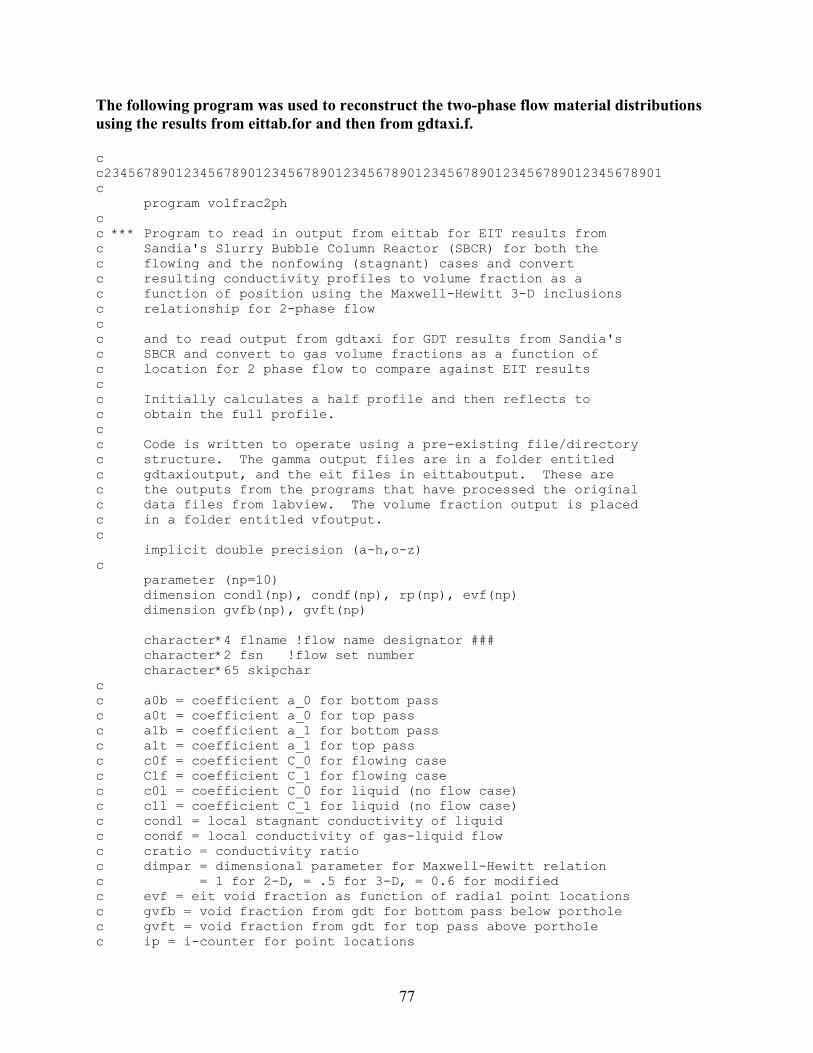
The following program was used to reconstruct the two-phase flow material distributions using the results from eittab.for and then from gdtaxi.f. c c2345678901234567890123456789012345678901234567890123456789012345678901 c program volfrac2ph c c *** Program to read in output from eittab for EIT results from c Sandia's Slurry Bubble Column Reactor (SBCR) for both the c flowing and the nonfowing (stagnant) cases and convert c resulting conductivity profiles to volume fraction as a c function of position using the Maxwell-Hewitt 3-D inclusions c relationship for 2-phase flow c c and to read output from gdtaxi for GDT results from Sandia's c SBCR and convert to gas volume fractions as a function of c location for 2 phase flow to compare against EIT results c c Initially calculates a half profile and then reflects to c obtain the full profile. c c Code is written to operate using a pre-existing file/directory c structure. The gamma output files are in a folder entitled c gdtaxioutput, and the eit files in eittaboutput. These are c the outputs from the programs that have processed the original c data files from labview. The volume fraction output is placed c in a folder entitled vfoutput. c implicit double precision (a-h,o-z) c parameter (np=10) dimension condl(np), condf(np), rp(np), evf(np) dimension gvfb(np), gvft(np) character*4 flname !flow name designator ### character*2 fsn !flow set number character*65 skipchar c c a0b = coefficient a_0 for bottom pass c a0t = coefficient a_0 for top pass c a1b = coefficient a_1 for bottom pass c a1t = coefficient a_1 for top pass c c0f = coefficient C_0 for flowing case c C1f = coefficient C_1 for flowing case c c0l = coefficient C_0 for liquid (no flow case) c c1l = coefficient C_1 for liquid (no flow case) c condl = local stagnant conductivity of liquid c condf = local conductivity of gas-liquid flow c cratio = conductivity ratio c dimpar = dimensional parameter for Maxwell-Hewitt relation c = 1 for 2-D, = .5 for 3-D, = 0.6 for modified c evf = eit void fraction as function of radial point locations c gvfb = void fraction from gdt for bottom pass below porthole c gvft = void fraction from gdt for top pass above porthole c ip = i-counter for point locations
77
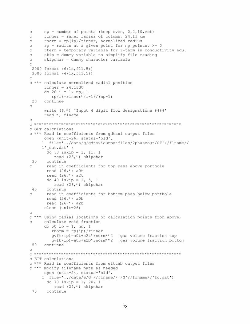
c np = number of points (keep even, 0,2,10,ect) c rinner = inner radius of column, 24.13 cm c rnorm = rp(ip)/rinner, normalized radius c rp = radius at a given point for np points, >= 0 c rterm = temporary variable for r-term in conductivity equ. c skip = dummy variable to simplify file reading c skipchar = dummy character variable c 2000 format (6(1x,f11.5)) 3000 format (4(1x,f11.5)) c c *** calculate normalized radial position rinner = 24.13d0 do 20 i = 1, np, 1 rp(i)=rinner*(i-1)/(np-1) 20 continue c write (6,*) 'Input 4 digit flow designatione ####' read *, flname c c ************************************************************ c GDT calculations c *** Read in coefficients from gdtaxi output files open (unit=26, status='old', 1 file='../data/g/gdtaxioutputfiles/2phaseout/GF'//flname// 1'_out.dat' ) do 30 iskip = 1, 11, 1 read (26,*) skipchar 30 continue c read in coefficients for top pass above porthole read (26,*) a0t read (26,*) a2t do 40 iskip = 1, 5, 1 read (26,*) skipchar 40 continue c read in coefficients for bottom pass below porthole read (26,*) a0b read (26,*) a2b close (unit=26) c c *** Using radial locations of calculation points from above, c calculate void fraction do 50 ip = 1, np, 1 rnorm = rp(ip)/rinner gvft(ip)=a0t+a2t*rnorm**2 !gas volume fraction top gvfb(ip)=a0b+a2b*rnorm**2 !gas volume fraction bottom 50 continue c c ************************************************************ c EIT calculations c *** Read in coefficients from eittab output files c *** modify filename path as needed open (unit=24, status='old', 1 file='../data/e/G'//flname//'/G'//flname//'fc.dat') do 70 iskip = 1, 20, 1 read (24,*) skipchar 70 continue
78

read (24,*) c0f read (24,*) c1f close (unit=24) c c *** Read in coefficients for stagnant, no-flow case c *** modify filename path as needed open (unit=25, status='old', 1 file='../data/e/G'//flname//'/G'//flname//'NFc.dat') do 80 iskip = 1, 20, 1 read (25,*) skipchar 80 continue read (25,*) c0l read (25,*) c1l close (unit=25) c c *** Calculate conductivities of both cases, and void fraction c dimpar =3.0d0/5.0d0 !for modified M-H do 90 ip = 1, np, 1 rterm = 2.0d0*(rp(ip)/rinner)**2-1.0d0 condf(ip)=1.0d0/c0f*(1.0d0+c1f*rterm) !flowing condl(ip)=1.0d0/c0l*(1.0d0+c1l*rterm) !nonflowing cratio=condf(ip)/condl(ip) evf(ip) = (1.0d0-cratio)/(1.0d0+dimpar*cratio) 90 continue c c *** Write output to file for eit and gdt volume fractions c as a function of radial position open (unit=28, status='new', 1 file='./vfresults/2ph/G'//flname//'/G'//flname//'vf.dat') write(6,*) 'rp, evf, gvft, gvfb, condl, condf' do 500 ip = np, 2, -1 write(28,2000) -rp(ip),evf(ip),gvft(ip),gvfb(ip), 1 condl(ip),condf(ip) 500 continue do 550 ip = 1, np, 1 write(28,2000) rp(ip),evf(ip),gvft(ip),gvfb(ip), 1 condl(ip),condf(ip) write(6,2000) rp(ip),evf(ip),gvft(ip),gvfb(ip), 1 condl(ip),condf(ip) 550 continue close (unit=28) c c--------------------------------------------- stop 'volfrac' end
79

The following program was used to reconstruct the three-phase flow material distributions using the results from both eittab.for and gdtaxi.f. c c2345678901234567890123456789012345678901234567890123456789012345678901 c program volfrac3ph c c *** Program to read in output from eittab for EIT results from c Sandia's Slurry Bubble Column Reactor (SBCR) for both the c flowing and the nonfowing (stagnant) cases and convert c resulting conductivity profiles to volume fraction as a c function of position using the Maxwell-Hewitt 3-D inclusions c relationship, modified for bimodal inclusions, for 3-phase c flow c c and to read output from gdtaxi for GDT results from Sandia's c SBCR c c and calculate the phase volume fractions as a function of radial c location for 3phase flow c c Initially calculates a half profile and then reflects to c obtain the full profile. c c Code is written to operate using a pre-existing file/directory c structure. The gamma output files are in a folder entitled c gdtaxioutput, and the eit files in eittaboutput. These are c the outputs from the programs that have processed the original c data files from labview. The volume fraction output is placed c in a folder entitled vfoutput. c implicit double precision (a-h,o-z) c parameter (np=10) dimension condl(np), condf(np), rp(np) dimension gvfb(np), gvft(np), gasf(np) dimension es(np), eg(np), el(np), f(np) c character*4 flname !flow name designator ### character*2 fsn !flow set number character*65 skipchar c c a0b = coefficient a_0 for bottom pass of GDT c a0t = coefficient a_0 for top pass of GDT c a1b = coefficient a_1 for bottom pass of GDT c a1t = coefficient a_1 for top pass of GDT c arterm = a coefficient in quadratic solution c brterm = b coefficient in quadratic solution c c0f = coefficient C_0 for flowing case (multiphase) c C1f = coefficient C_1 for flowing case (multiphase) c c0l = coefficient C_0 for liquid (no flow case) c c1l = coefficient C_1 for liquid (no flow case) c condl = local stagnant conductivity of liquid c condf = local conductivity of multiphase flow c cratio = conductivity ratio
80

c crterm = c coefficient for quadratic solution c dimpar = dimensional parameter for Maxwell-Hewitt relation c = 1 for 2-D, = .5 for 3-D, = 0.6 for modified c dmslsg = attenuation coefficient ratio =(mu_s-mu_l)/(mu_s-mu_g) c dmlgsg = attenuation coefficient ratio =(mu_l-mu_g)/(mu_s-mu_g) c dmsgsl = attenuation coefficient ratio =(mu_s-mu_g)/(mu_s-mu_l) c dmlgsl = attenuation coefficient ratio =(mu_l-mu_g)/(mu_s-mu_l) c eg = gas volume fraction c el = liquid volume fraction c es = solid volume fraction c f = normalized radial attenuation coefficient, average c flname = flow name (designation) c fsn = flow set name c gasf = average gas fraction from GDT measurement c gvfb = void fraction from gdt for bottom pass below porthole c gvft = void fraction from gdt for top pass above porthole c ip = i-counter for point locations c np = number of points (keep even, 0,2,10,ect) c rinner = inner radius of column, 24.13 cm c rnorm = rp(ip)/rinner, normalized radius c rp = radius at a given point for np points, >= 0 c rterm = temporary variable for r-term in conductivity equ. c skipchar = dummy character variable to skip lines c 2000 format (5(1x,f11.5)) 3000 format (4(1x,f11.5)) c c *** calculate radial position values rinner = 24.13d0 do 20 i = 1, np, 1 rp(i)=rinner*(i-1)/(np-1) 20 continue c c *** input flow sets for three phase flow, GD=0%, GS=4%, G2=8% loading c *** input 4 digit flow designation, e.g., 1015 for 10 cm/s and 15psia write (6,*) 'Input which flow set, GD, GS, G2' read *, fsn write (6,*) 'Input 4 digit flow designation ####' read *, flname c c ************************************************************ c GDT calculations c *** Read in coefficients from gdtaxi output files c *** modify input filename path as required c open (unit=26, status='old', 1 file='../data/g/gdtaxioutputfiles/3phaseout/'//fsn//flname// 1'_out.dat' ) do 30 iskip = 1, 11, 1 read (26,*) skipchar 30 continue c *** read in coefficients for top pass above porthole read (26,*) a0t read (26,*) a2t do 40 iskip = 1, 5, 1 read (26,*) skipchar 40 continue
81

c *** read in coefficients for bottom pass below porthole read (26,*) a0b read (26,*) a2b close (unit=26) c c *** Using radial locations of calculation points from above, c *** calculate void fraction with GDT data do 50 ip = 1, np, 1 rnorm = rp(ip)/rinner gvft(ip)=a0t+a2t*rnorm**2 !gas volume fraction top gvfb(ip)=a0b+a2b*rnorm**2 !gas volume fraction bottom 50 continue c c ************************************************************ c EIT calculations c *** Read in coefficients from eittab output files c *** modify input filename path as required open (unit=24, status='old', 1 file='../data/e/3Peit/'//fsn//flname//'/res/'//fsn// 1flname//'eittabr.dat' ) do 70 iskip = 1, 20, 1 read (24,*) skipchar 70 continue read (24,*) c0f read (24,*) c1f close (unit=24) c c *** Use EIT results for no flow case for 0% loading, dirty water c *** for all three phase runs to obtain similar temperatures and no c *** solids open (unit=25, status='old', 1 file='../data/e/3Peit/GD1030/res/GD1030NFeittabr.dat' ) do 80 iskip = 1, 20, 1 read (25,*) skipchar 80 continue read (25,*) c0l read (25,*) c1l close (unit=25) c c *** Calculate conductivities of both cases, and void fraction c *** attenuation ratios dmslsg=(mu_s-mu_l)/(mu_s-mu_g) dmslsg=(0.0866d0-0.0856d0)/(0.0866d0-0.0000819d0) dmlgsg=(0.0856d0-0.0000819d0)/(0.0866d0-0.0000819d0) dmsgsl=(0.0866d0-0.0000819d0)/(0.0866d0-0.0856d0) dmlgsl=(0.0856d0-0.0000819d0)/(0.0866d0-0.0856d0) c dimpar = 0.6d0 !=3.0d0/5.0d0 for modified Maxwell-Hewitt do 90 ip = 1, np, 1 gasf(ip)=(gvft(ip)+gvfb(ip))/2.0d0 !average gas fraction f(ip)=1.0d0-gasf(ip) !(average f term) rterm = 2.0d0*(rp(ip)/rinner)**2-1.0d0 condf(ip)=1.0d0/c0f*(1.0d0+c1f*rterm) !flowing condl(ip)=1.0d0/c0l*(1.0d0+c1l*rterm) !nonflowing cratio=condf(ip)/condl(ip) c cratio=condf(ip)/(condl(ip)*0.71d0) !vary liquid conductivity c arterm=1.0d0+(dmslsg*dimpar-dmlgsg*dimpar**2)*cratio
82
brterm=-2.0d0+dmlgsg*f(ip)+ 1(dmslsg-dimpar+dmlgsg*(1.0d0-f(ip))*dimpar**2)*cratio crterm=1.0d0-dmlgsg*f(ip)+ 1(-dmslsg+dmlgsg*(1.0d0-f(ip))*dimpar)*cratio c eg(ip)=(-brterm-dsqrt(brterm**2-4.0d0*arterm*crterm)) 1/(2.0d0*arterm) el(ip)=dmsgsl-dmlgsl*f(ip)-dmsgsl*eg(ip) es(ip)=1.0d0-eg(ip)-el(ip)c 90 continue c c *** Write output to file for eit and gdt volume fractions c as a function of radial position c *** modify filename path as needed open (unit=28, status='new', 1 file='./vfresults/3ph/'//fsn//flname//'/out2/' 1//fsn//flname//'out.dat' ) open (unit=29, status='new', 1 file='./vfresults/3ph/'//fsn//flname//'/'//fsn//flname// 1'vf3.dat' ) c------------------------------------------- write(6,*) 'rp, gvft, gvfb, condl, condf' do 500 ip = np, 2, -1 write(28,2000) -rp(ip),gvft(ip),gvfb(ip),condl(ip),condf(ip) write(6,2000) -rp(ip),gvft(ip),gvfb(ip),condl(ip),condf(ip) 500 continue do 550 ip = 1, np, 1 write(28,2000) rp(ip),gvft(ip),gvfb(ip),condl(ip),condf(ip) write(6,2000) rp(ip),gvft(ip),gvfb(ip),condl(ip),condf(ip) 550 continue c--------------------------------------------- write(6,*) 'rp, eg, el, es' do 600 ip = np, 2, -1 write(29,3000) -rp(ip),eg(ip),el(ip),es(ip) write(6,3000) -rp(ip),eg(ip),el(ip),es(ip) 600 continue do 650 ip = 1, np, 1 write(29,3000) rp(ip),eg(ip),el(ip),es(ip) write(6,3000) rp(ip),eg(ip),el(ip),es(ip) 650 continue close (unit=28) close (unit=29) c c--------------------------------------------- stop 'volfrac' end
83

Distribution Sandia 1 MS0824 A.C. Ratzel, 9110 3 MS0826 J.R. Torczynski, 9113 1 MS0826 Manager, 9113 3 MS0834 S.G. Liter, 9112 1 MS0834 T.J. O’Hern, 9112 1 MS0834 M.R. Prairie, 9112 1 MS0834 P.R. Tortora, 9112 1 MS0834 S.M. Trujillo, 9112 1 MS0841 T.C. Bickel, 9100 1 MS0886 N.B. Jackson, 01812 1 MS0188 LDRD Office, 1011 1 MS9018 Central Technical Files,
8945-1 2 MS0899 Technical Library, 9616 1 MS0612 Review and Approval
Desk, for DOE/OSTI
External 3 Professor Kim A. Shollenberger California Polytechnic State University Mechanical Engineering Department San Luis Obispo, CA 93407 3 Professor Steven L. Ceccio University of Michigan Mechanical Engineering Department Ann Arbor, MI 48109-2125 1 Dr. Darin L. George Southwest Research Institute Mechanical and Fluids Engineering 6220 Culebra Road P.O. Drawer 28510 San Antonio, Texas 78228-0510
1 Professor Milorad P. Dudukovic Washington University Chemical Engineering Department St. Louis, MO 63130-4899 1 Dr. Bernard A. Toseland Air Products and Chemicals, Inc. 7201 Hamilton Boulevard Allentown, PA 18195-1501 1 Mr. John Winslow U.S. Department of Energy National Energy Technology
Laboratory P.O. Box 10940 Pittsburgh, PA 14236
84


![Electrical Principles 1 1 G5 - ELECTRICAL PRINCIPLES [3 exam questions - 3 groups] G5A - Reactance; inductance; capacitance; impedance; impedance matching](https://img.dokumen.tips/doc/110x75/56649f585503460f94c7d788/electrical-principles-1-1-g5-electrical-principles-3-exam-questions-3.jpg)