Electrical Impedance Imaging of

Corrosion on a Partially

Accessible 2-Dimensional Region

An Inverse Problem in Non-Destructive Testing

Court Hoang 1 and Katherine Osenbach 2

Abstract

In this paper we examine the inverse problem of determining the

amount of corrosion on an inaccessible surface of a two-dimensional re-

gion. Using numerical methods, we develop an algorithm for approximat-

ing corrosion profile using measurements of electrical potential along the

accessible portion of the region. We also evaluate the effect of error on the

problem, address the issue of ill-posedness, and develop a method of regu-

larization to correct for this error. An examination of solution uniqueness

is also presented.

1Pomona College2The University of Scranton

1

1 Introduction

The ability to determine the size and location of defects on the interior of an

object without destroying the object’s integrity has many useful applications in

industry today. Two of many methods for attacking this problem are impedance

imaging and thermal imaging. In this paper, we will examine the use of steady

state electrical impedance imaging to detect corrosion on the back surface of a

region.

We will consider a region, Ω, that has a readily accessible top surface, but

a completely inaccessible back surface. Our goal is to use measurements of

electrical potential on the accessible surface to recover the profile of the corrosion

on the back surface. That is, we will investigate how a corroded region, with a

different electrical conductivity than that of the non-corroded region, impedes

the flow of current from one portion of the surface to another. We will then

use these impedance effects to reconstruct the corrosion profile knowing the

conductivity of the corroded region, the input current profile, and the potential

on the accessible surface.

2 The Forward Problem

Let Ω be a region in R2 defined in the following way: Ω = (x, y) : y ∈ [0, 1], x ∈(−∞,∞) (see Figure 1). Let Γ denote the upper boundary of Ω where y = 1.

Let the curve y = S(x) represent the upper boundary of a region Ω− ⊆ Ω such

that S(x) has compact support. Let Ω+ = Ω\Ω−. We assume Ω+ has electrical

conductivity equal to 1. We also assume Ω−, which represents a region of cor-

rosion along the back surface, has constant electrical conductivity γ not equal

to 1.

A time-independent electrical flux, g, is applied to Γ. Assuming that the

problem is steady-state, we then have functions of electrical potential, u+ and

u−, in Ω+ and Ω−, respectively, satisfying the following partial differential equa-

tions (following from a standard model):

∆u+ = 0, on Ω+

∆u− = 0, on Ω−, (2.1)

where ∆u is the Laplacian of u. We also have the following boundary conditions:

2

Figure 1: Diagram of the problem set-up.

∂u+

∂~n= ∇u+ · ~n = g , on Γ

∂u+

∂~n= ∇u+ · ~n = 0, on y = 0

∂u−

∂~n= ∇u− · ~n = 0, on y = 0

u+ = u−, on y = S(x) (2.2)

∂u+

∂~n= γ

∂u−

∂~n(2.3)

where ~n is an unit outward normal vector on Γ, y = 0, and y = S(x). Equation

(2.1) is known as Laplace’s Equation. Functions that satisfy this equation are

said to be harmonic.

Let us first consider the case where Ω− = ∅, that is there is no corrosion on

the back surface of Ω. In this case, we will call the potential resulting from a

non-corroded back surface u0; note that u0 will be defined on all of Ω. Now let

us consider the case where Ω− 6= ∅, that is, some portion of the back surface of

Ω is corroded.

This forward problem involves solving a system of partial differential equa-

tions given in equation (2.1) for the steady state electrical potential functions

u+ and u− that satisfy the given boundary data detailed in equation (2.2). This

forward problem is not the problem we analyzed. Instead, we will be investigat-

ing the following inverse problem: given information about u+ on Γ, with known

constant conductivity γ in Ω−, and input flux g on Γ, we wish to approximate

3

the function y = S(x).

3 Preliminary Information

Green’s second identity will prove to be a useful tool for attacking the inverse

problem. Let us recall Green’s Second Identity: for any bounded region D ⊂ R2,

with sufficiently smooth boundary ∂D, if u, v ∈ C2(D ∪ ∂D), then∫∫

D

(u∆v − v∆u) dA =∫

∂D

(u∂v

∂~n− v

∂u

∂~n) ds (3.1)

where ds is the arc length element and ~n is the outward unit normal to ∂D. In

our analysis, the function v(x, y), which we refer to as the “test function”, will

be chosen to be harmonic. Green’s second identity is a direct consequence of

the Divergence Theorem, and will be used as the primary means of recovering

the function y = S(x).

4 Uniqueness

We will now discuss uniqueness for this inverse problem. In the linearized version

of this problem (see Section 6), uniqueness of the corrosion profile S(x) holds

for a single measurement of data along the accessible surface Γ; however, in the

non-linear version of the problem, it is very unlikely that a single measurement

would assure uniqueness of S [1]. Though we do not have a complete uniqueness

result, we show here that, in the non-linear version, if two profiles S1 and S2

generate the same data for u+ along Γ, then S1 and S2 must have a non-zero

point of intersection on their supported domains.

Suppose we have a region Ω ∈ R2, bounded above by Γ = (x, y) : y = 1,and below by the line y = 0 (see Figure 2(a)). Given a function u1(x, y) defined

on Ω and a curve y = S1(x) 6≡ 0 with compact support, suppose that the con-

ductivity is 1 above S1(x) and γ 6= 1 below S1(x). Call u1 above S1(x) u+1 , and

below S1(x), call it u−1 . Suppose also that u1 satisfies the following conditions:

4

(a) Setup for u1 with conductivity equal to 1 on

Ω1 and conductivity γ 6= 1 under y = S1(x).

(b) Setup for u2 with conductivity 1 on

Ω2 and conductivity γ 6= 1 under y = S2(x).

Figure 2: Problem setup for u1 and u2.

∆u1 = 0 for y > S1(x) and y < S1(x),∂u1∂~n = g on Γ,

∂u1∂~n = 0 when y = 0,

u+1 = u−1 on S1(x) (i.e., u1 is continuous over S1(x)), and

∂u+1

∂~n = γ∂u−1∂~n . (4.1)

Now, suppose we have another function u2(x, y) on Ω and another curve

S2(x) 6≡ 0, also with compact support, such that u2 satisfies the same condi-

tions as u1 with respect to S2 (using the same boundary flux g and with the

same value for γ under S2; see Figure 2(b)). Let Ω1, Ω2 ⊆ Ω be the respective

regions on which u1 and u2 have conductivity equal to 1 (see Figure 2). For

the sake of simplicity, we assume that S1 and S2 are non-zero only on the in-

tervals (a, b) and (c, d), respectively, and that they intersect at most once on

(a, b) ∪ (c, d) (see Figures 2, 3). Let D1 be the region enclosed by S1 and S2

when S1 > S2 (i.e., the region below S1 and above S2); let D2 be the region

enclosed by S1 and S2 when S1 < S2 (i.e., the region below S2 and above S1);

let D3 be the region below both S1 and S2 (see Figure 3). Note that any given

Dk may be empty.

Claim. If u1 = u2 on any open portion of Γ, then there exists x ∈ R such that

0 6= S1(x) = S2(x); that is, the non-zero portions of the graphs of S1 and S2

5

must intersect.

Proof. We begin with a statement of the following standard “unique continua-

tion” lemma.

Lemma 1. Given a connected region Ω with C2 boundary and

functions u1, u2 with ∆u1,2 = 0 in Ω, ∂u1∂~n = ∂u2

∂~n on an open

subset Γ of the boundary of Ω, and u1 = u2 on Γ, then u1 = u2

everywhere in Ω.

Now, suppose we have u1 = u2 on some open portion σ of Γ. Since u1 = u2

on σ, and because ∂u1∂~n = ∂u2

∂~n = g on all of Γ, it follows (by Lemma 1) that

u+1 = u+

2 everywhere on Ω1 ∩ Ω2. (4.2)

In this proof, we consider two cases: one in which S1 and S2 have disjoint

supports (see Figure 3(b)); and one in which S1 ≥ S2 everywhere (analogous to

the case in which S2 ≥ S1; see Figure 3(c)).

Case 1

In the first case, where (a, b) ∩ (c, d) = ∅, we note first that D3 = ∅ (see

Figure 3(b)). Looking at D1, we know that ∂u1∂~n = ∂u2

∂~n = 0 along the back

surface y = 0, and we also know by (4.1) and (4.2) that u−1 = u+1 = u+

2 on

S1(x). Thus, we have the normal derivatives of u−1 and u+2 equal to each other

on part of the boundary of D1, namely, on y = S1(x), and u−1 = u+2 on another

part of the boundary, namely, on y = 0. These two conditions are enough to

ensure that, because both u1 and u2 satisfy Laplace’s equation,

u1 = u2 everywhere in D1. (4.3)

Similarly, we know that

u1 = u2 everywhere in D2. (4.4)

Now, we know that D1 or D2 (or both) is non-empty. Without loss of gener-

ality, assume that D1 6= ∅. Then, by (4.3), we know that u−1 = u+2 everywhere

in D1; by (4.2), u+1 = u+

2 on Ω1 ∩ Ω2. Thus u+1 = u−1 = u+

2 on Ω2 (since u2 is

smooth over S1), and so ∂u+1

∂~n = ∂u−1∂~n on Ω2, contradicting our hypothesis (4.1)

that ∂u+1

∂~n = γ∂u−1∂~n (because γ 6= 1). We conclude that S1 and S2 cannot have

6

(a) With one non-zero intersection between S1

and S2.

(b) Figure for Case 1 ((a, b) ∩ (c, d) = ∅); note

that here, D3 = ∅.

(c) Figure for Case 2 (S1 ≥ S2 everywhere); note

that here, D2 = ∅.

Figure 3: Possible cases when S1 and S2 intersect non-trivially at most once.

disjoint support.

Case 2

In the second case, where S1 ≥ S2 everywhere, we first note that D2 = ∅,and that D3 ⊂ Ω\Ω1 (see Figure 3(c)). Defining the functions γ1 and γ2 in

accordance with our problem setup by

γk =

1 in Ωk,

γ in Ω\Ωk,

we can restate the first condition (Laplace’s equation) in our original boundary

value problem (4.1) as

∇ · (γ1∇u1) = 0 in Ω; (4.5)

we can do the same for the boundary value problem with u2 and S2.

Suppose the solutions u1,2 to these BVPs have Dirichlet boundary condition

u1 = u2 = f along ∂Ω = Γ ∪ y = 0, the boundary of Ω, for some f ∈ C1

(we know that u1 and u2 must be defined by the same f by (4.2)). By Dirich-

7

let’s Principle (see [2]), as solutions to these BVPs, u1 and u2 also minimize,

respectively, the functionals

Q1(φ) =∫

Ω

γ1

∣∣∇φ∣∣2 dA,

Q2(φ) =∫

Ω

γ2

∣∣∇φ∣∣2 dA, (4.6)

where φ is any function satisfying φ = f on ∂Ω.

Consider the quantity∫

∂Ω

uk∂uk

∂~n, k = 1, 2.

This integral gives the power necessary to maintain the electrical current in Ω

for u1 or u2. Now, along Γ, u1 = u2 (4.2), and ∂u1∂~n = ∂u2

∂~n = g (4.1). We also

know by (4.1) that ∂u1∂~n = ∂u2

∂~n = 0 along the back surface y = 0. Thus, for all

of ∂Ω, we have

∫

∂Ω

u1∂u1

∂~nds =

∫

∂Ω

u2∂u2

∂~nds, (4.7)

which implies

∫

Ω

γ1

∣∣∇u1

∣∣2 dA =∫

Ω

γ2

∣∣∇u2

∣∣2 dA

or, equivalently,

Q1(u1) = Q2(u2). (4.8)

Suppose that γ < 1 (the case where γ > 1 yields an analogous contradiction).

Then, because D3 ⊂ D1 (i.e., the area under S1 is greater than that of S2),

γ1 ≤ γ2 everywhere on Ω, and equality holds everywhere except on D1. Then,

for any φ with φ = f on ∂Ω, it must be that

∫

Ω

γ1

∣∣∇φ∣∣2 dA ≤

∫

Ω

γ2

∣∣∇φ∣∣2 dA. (4.9)

In fact, equality only holds in (4.9) if φ is constant on D1: since equality

between γ1 and γ2 holds except on D1, we would need to have

∫

D1

γ1

∣∣∇φ∣∣2 dA =

∫

D1

γ2

∣∣∇φ∣∣2 dA,

or ∫

D1

γ∣∣∇φ

∣∣2 dA =∫

D1

1 ·∣∣∇φ

∣∣2 dA

8

(since γ1 = γ, γ2 = 1 on D1), so∫

D1

(γ − 1)∣∣∇φ

∣∣2 dA = 0.

Since γ 6= 1, then |∇φ | = 0, so φ must be constant on D1.

Because u2 satisfies Laplace’s equation, we cannot have u2 constant on D1

or it would be constant everywhere on Ω. Thus, by (4.9), we may say that

Q2(u2) =∫

Ω

γ2

∣∣∇u2

∣∣2 dA >

∫

Ω

γ1

∣∣∇u2

∣∣2 dA. (4.10)

Because u1 minimizes Q1(u1) as defined in (4.6), we know that

Q1(u1) =∫

Ω

γ1

∣∣∇u1

∣∣2 dA ≤∫

Ω

γ1

∣∣∇u2

∣∣2 dA. (4.11)

Combining (4.10) and (4.11) yields

Q2(u2) >

∫

Ω

γ1

∣∣∇u2

∣∣2 dA ≥ Q1(u1), (4.12)

contradicting (4.8).

Thus, in either case, we reach a contradiction, and so there must be a non-

zero point of intersection between S1 and S2; more precisely, S1 and S2 cannot

have disjoint supports, and neither can lie entirely above the other.

5 Recovering S(x)

Our goal is to reconstruct the function y = S(x) which determines the corroded

surface Ω−. To this end, we will use Green’s second identity (3.1), with a test

function v(x, y) satisfying the following conditions:

∆v(x, y) = 0,

∂v

∂~n= 0 when y = 0. (5.1)

Both u(x, y) and v(x, y) are harmonic functions. The left hand side of equa-

tion (3.1) thus becomes identically 0; applying this on the region Ω1 and sub-

stituting the fact that ∂u+

∂~n = g on Γ yields:

0 =∫

Γ

u+ ∂v

∂~n− vg ds−

∫

S

u+ ∂v

∂~n− v

∂u+

∂~nds (5.2)

9

On the region Ω−, knowing that ∂u−∂~n = 0 on y = 0 and ∂u−

∂~n = 1γ

∂u+

∂~n on

y = S(x), we will again apply Green’s second identity to obtain:

0 =∫

y=S(x)

u−∂v

∂~n− v

1γ

∂u+

∂~nds−

∫

y=0

u−∂v

∂~n− v

1γ

∂u+

∂~nds (5.3)

The goal is to obtain an equation in which we have known, or calculable, quan-

tities equal to the unknown S function. To this end, add equations (5.2) and

(5.3) to obtain the following:∫

Γ

u+ ∂v

∂~n− vg ds−

∫

y=0

u2∂v

∂~nds =

∫

y=S(x)

(u+ − u−)∂v

∂~n+ v(1− 1

γ)∂u+

∂~nds.

Because we chose the test function v such that ∂v∂~n = 0 on y = 0, this gives

the following simplified equation:∫

Γ

u+ ∂v

∂~n− vg ds−

∫

y=0

u−∂v

∂~nds =

∫

y=S(x)

v(1− 1γ

)∂u+

∂~nds. (5.4)

An alternate form of equation (5.4) can be obtained by multiplying equation

(5.3) by γ and then adding it to equation (5.2). This results in the following:∫

Γ

u+ ∂v

∂~n−vg ds−γ

∫

y=0

u−∂v

∂~nds =

∫

y=S(x)

γu−∂v

∂~n−v

∂u+

∂~n−u+ ∂v

∂~n+v

∂u+

∂~nds.

But u+ = u− on y = S(x), and we chose v such that ∂v∂~n = 0 on S; therefore,

we have: ∫

Γ

(u+ ∂v

∂~n− vg

)ds

︸ ︷︷ ︸RG(v)

=∫

y=S(x)

(γ − 1)u+ ∂v

∂~nds (5.5)

The left side of equation (5.5) is often referred to as the reciprocity gap

integral. We will hereby refer to it as RG(v) throughout the remainder of this

paper. RG(v) is a computable quantity for any chosen harmonic test function

v from the known boundary data u+ and input flux g. We thus have

RG(v) =∫

y=S(x)

(γ − 1)u+ ∂v

∂~nds (5.6)

Let us write equation (5.6) out a bit more explicitly. A unit normal vector

to the curve y = S(x), pointing upward, is of the following form:

~n =< −S′(x), 1 >√

1 + (S′(x))2

10

the ds arc length factor is:

ds =√

1 + (S′(x))2 dx (5.7)

Multiplying ∂v∂~n = ∇v · ~n by the differential ds yields:

∂v

∂~nds =

−S′(x) ∂v∂x + ∂v

∂y√1 + (S′(x))2

·√

1 + (S′(x))2 dx = −S′(x)∂v

∂x+

∂v

∂ydx (5.8)

Substituting this into the right side of equation (5.6) we obtain:

RG(v) = (γ−1)∫ ∞

−∞−u+(x, S(x))S′(x)

∂v

∂x(x, S(x))+u+(x, S(x))

∂v

∂y(x, S(x)) dx

(5.9)

We now have reached the desired goal of known quantities on one side of the

equation, and the unknown function S on the other. Given information about

the potential on Γ, the electrical conductivity γ in Ω−, the general procedure is

to use equation (5.9), with an appropriate variety of test functions v, to collect

information about the function y = S(x) which defines the corroded region Ω−.

One difficulty is that the function S appears inside u+, a quantity not know to

us. The problem can be overcome by linearizing, as we show below.

6 Linearization

How can we use (5.9) to obtain an accurate approximation of the S function? To

answer this question will implement the following two procedures - linearization

and regularization.

We will begin with the process of linearization (regularization will be dis-

cussed in Section 12). Recall right side of equation (5.9). We will make the as-

sumption that the corrosion profile is close to zero, that is, assume that S = εS0

for some “base profile” S0. Let us first examine the case where ε = 0. If ε = 0

then S = 0, and we have:

(γ − 1)∫ ∞

−∞u(x, 0)vy(x, 0) dx = 0. (6.1)

The case where ε > 0, requires the following intuitive approximation: u+(x, εS0(x)) ≈u0(x, εS0(x)) for ε small. This approximation can be quantitatively justified,

11

but this is beyond the scope of our work. Under this approximation, however,

the right side of equation (5.9) becomes:

(γ − 1)∫ ∞

−∞u0(x, εS0(x))

[− εS′0(x)vx(x, εS′0(x)) + vy(x, εS′0(x))

]dx. (6.2)

We will now perform a Taylor series expansion on the right side of the expres-

sion in (6.2) about ε = 0 in order to linearize the problem for further analysis.

The Taylor series expression for u0(x, εS0(x)) about ε = 0 is:

u0(x, εS0(x) = u0(x, 0) + ε∂u0

∂y|(x,0) S0(x) +

12ε2 ∂2u0

∂2y|(x,0) +O(ε3)

= u0(x, εS0(x)) +12ε2 ∂2u0

∂2y|(x,0) +O(ε3),

because of the insulating boundary condition ∂u0∂y

∣∣(x,0)

= 0.

The Taylor series expression for −εS′0(x)vx(x, εS0(x)) is

−εS′0(x)vx(x, εS0(x)) = −εS′0(x)vx(x, 0)− ε2S′0(x)vxy(x, 0)S0(x)−O(ε3).

The Taylor series expression for vy(x, εSo(x) is

vy(x, εS0(x) = vy(x, 0) + εS0(x)vyy(x, 0) +ε2

2(S0(x))2vyyy(x, 0) + O(ε3).

We can now substitute these Taylor expressions into equation (6.2) to obtain:

(γ−1)∫ ∞

−∞

[u0(x, 0)+ε

∂u0

∂y|(x,0) S0(x)+

12ε2 ∂2u0

∂2y|(x,0) +O(ε3)

][−εS′0(x)vx(x, 0)

− ε2S′0(x)vxy(x, 0)S0(x)+vy(x, 0)+εS0(x)vyy(x, 0)+ε2

2(S0(x))2vyyy(x, 0)+O(ε3)

]dx.

Multiplying through, and grouping terms according to order of ε, we have:

(γ−1)∫ ∞

−∞ε(u0(x, 0)

[S0(x)vyy(x, 0)−S′0(x)vx(x, 0)

]+S0(x)vy(x, 0)

∂u0

∂y|(x,0)

)+O(ε2) dx.

Note that the zero-order term (γ−1)∫∞−∞ u0(x, 0) ·vy(x, 0) is zero by our choice

of v and equation (6.1).

12

Terms of order ε2 and higher can be ignored for ε small without greatly

affecting the approximation. Under this assumption, the right side of (5.9)

becomes

(γ−1)ε∫ ∞

−∞u0(x, 0)

[S0(x)vyy(x, 0)−S′0(x)vx(x, 0)

]+S0(x)vy(x, 0)

∂u0

∂y|(x,0) dx.

Now recall our choice of v(x, y) such that vy(x, 0) = 0. Equation (5.9) becomes

RG(v) ≈ (γ − 1)ε∫ ∞

−∞u0(x, 0)

[S0(x)vyy(x, 0)− S′0(x)vx(x, 0)

]dx. (6.3)

Since v(x, y) satisfies Laplace’s equation, we know that vyy(x, y) = −vxx(x, y)

on Ω+ and Ω−, and so we can substitute in the right side of the approximation

(6.3) to obtain:

(γ − 1)ε∫ ∞

−∞−u0(x, 0)[S0(x)vxx(x, 0) + S′0(x)vx(x, 0)] dx.

Letting h(x) = v(x, 0), we can use the product rule in one dimension to obtain:

−(γ − 1)ε∫ ∞

−∞u0(x, 0)

[S0(x)h′′(x) + S′0(x)h′(x)

]dx

= −(γ − 1)ε∫ ∞

−∞u0(x, 0)

d

dx

[S0(x)h′(x)

]dx.

Using differentiation by parts,∫

udv = uv − ∫vdu, with u = u0(x, 0) and

dv = ddx [S0(x)h′(x)], we get:

−(γ − 1)ε[u0(x, 0)S0(x)h′(x)

∣∣∣∞

−∞+

∫ ∞

−∞

∂u0

∂x|(x,0) S0(x)h′(x) dx

].

Substituting v(x, 0) = h(x) back in yields:

−(γ − 1)ε[u0(x, 0)S0(x)vx(x, 0)

∣∣∣∞

−∞+

∫ ∞

−∞

∂u0

∂x|(x,0) S0(x)vx(x, 0) dx

]. (6.4)

Assuming that our function S0(x) has compact support, the first term of (6.4)

is zero when evaluated from −∞ to ∞. We are left with:

−(γ − 1)ε∫ ∞

−∞

∂u0

∂x(x, 0)S0(x)vx(x, 0) dx. (6.5)

13

Finally, we can substitute (6.5) back into equation (5.9) to obtain:

RG(v) ≈ −(γ − 1)ε∫ ∞

−∞

∂u0

∂x(x, 0)S0(x)vx(x, 0) dx.

= (1− γ)∫ ∞

−∞

∂u0

∂x(x, 0)

∂vk

∂x(x, 0)S(x) dx (6.6)

Equation (6.6) is the fully linearized version of our original reciprocity gap

equation (5.9). Once again, note that RG(v) is calculable: we choose v(x, y),

and we can compute u0(x, y) on Γ. Thus the linearized equation allows us to

numerically solve for the function S that defines the corrosion.

We should note that it can be shown, using an integration-by-parts argument

similar to the reciprocity gap argument above, that we can also compute RG(v)

as

RG(v) =∫

Γ

(u

∂v

∂n− vg

)ds (6.7)

where u is the function defined on Ω = (−∞,∞)× (0, 1) that satisfies

4u = 0 in Ω (6.8)∂u

∂n= 0 on y = 1 (6.9)

∂u

∂n= − ∂

∂x

(S0(x)

∂u0

∂x(x, 0)

)on y = 0. (6.10)

The problem (6.8)-(6.10) is the linearized (with respect to S = 0) version of the

original problem stated in Section 2.

7 Approximating the Corrosion Profile

In the previous section, we derived a linearized version (6.6) of our original

reciprocity gap integral equation (5.9), when the appropriate test function v

is chosen. Using this linearized equation, we can use numerical methods to

produce a function approximating the curve y = S(x), and thus we can obtain

an approximate image of the corrosion profile on the inaccessible surface. To

this effect, we group the known quantities on the right side of equation, which

becomes

RG(v) = −(γ − 1)∫ ∞

−∞w(x)S(x) dx, (7.1)

14

where w(x) = ∂u0∂x (x, 0)vx(x, 0). As we choose test functions vj , we refer to their

respective w functions as wj (i.e., wj(x) = ∂u0∂x (x, 0)∂vj

∂x (x, 0)).

We choose a number, n, of test functions vj , j = 1, ..., n, and we obtain a

system of n linear equations:

RG(v1) = (1− γ)∫ ∞

−∞w1(x)S(x) dx,

RG(v2) = (1− γ)∫ ∞

−∞w2(x)S(x) dx,

...

RG(vn) = (1− γ)∫ ∞

−∞wn(x)S(x) dx. (7.2)

Now, we know RG(vj) and wj(x) for j = 1, ..., n. We wish to find a function

S(x) that satisfies these equations and minimizes ‖S(x)‖2, the L2-norm of S(x).

We use the L2-norm because it produces a more elegant solution, and because

it gives a lower-bound for severity of the corrosion. It is shown in the following

section that such an S is unique and of the form

S(x) =n∑

j=1

cjwj(x), (7.3)

where the numerical coefficients cj are as yet unknown. Substituting (7.3) into

(7.2), we obtain a system of n equations with n unknowns cj . Solving this

system of equations yields the cj , giving us an approximation for S(x) as a

linear combination of the functions wj(x).

7.1 Proof of How to Find the Minimum Norm Linear Ap-

proximation of The Function y = S(x)

Let S be a function defined on an interval I. Suppose:∫

I

wk(x)S(x) dx = ak (7.4)

for k = 1 to n, where the wk and ak functions are known. Also recall that the

L2(I) norm is given by

‖S(x)‖2 =

√∫

I

S2(x) dx,

15

and that the inner product of two functions f, g ∈ L2(I) is

< f, g >=∫

I

f(x)g(x) dx,

assuming, as we are, that the functions are real-valued.

Claim: If the wk ∈ L2(I), then the function S which is consistent with the

data in equations (7.1) and has the smallest L2-norm is of the form:

S(x) =n∑

k=1

λkwk(x) (7.5)

for some constants λk.

Proof. Assume S(x) is defined on an interval I and we are given (7.4). The

set of functions w1, w2, ..., wn can be extended to a basis for L2(I) by adding

wn+1, wn+2, ... These additional basis functions can be chosen such that they

are orthogonal to the first n functions. Thus any function S ∈ L2(I) can be

expressed as:

S(x) =n∑

j=1

λjwj(x) + r(x) (7.6)

where r(x) =∑∞

j=n+1 λjwj(x). Note that < r,wj >= 0 for j ≤ n.

Then (7.4) becomes:n∑

j=1

< wk, wj > λj = ak

which is a system of n equations with n unknowns λj , j = 1 to j = n. This

system uniquely determines the λj , at least if the equations are not singular. So

the first n of the λj in (7.6) are forced by the constraints. We want to choose

the remaining λj to minimize ‖S‖2. But we can see that:

‖S‖22 =

∥∥∥∥∥∥

n∑

j=1

λjwj

∥∥∥∥∥∥

2

+ ‖r‖2

Since the λ1, ..., λn are fixed, ‖S‖22 can only be changed by changing ‖r‖. To

minimize ‖S‖2, we of course take r = 0. Thus the function S which is consistent

with the data and has the smallest L2-norm is of the form:

S(x) =n∑

k=1

λkwk(x)

16

.

8 Program Outline

We designed a Maple program to approximate the function y = S(x) using the

calculations shown above. For any given set of data taken on the accessible

surface Γ of Ω, the program generates a function S(x) that approximates the

contour of the corrosion present on the inaccessible back surface of Ω. The

data is generated assuming a particular input flux g thus also determining the

function u0(x, y).

We must first generate the system of equations to be solved by calculating

the RG(v) values and the w(x) functions. To this end, we must choose test

functions v(x, y) that satisfy the conditions expressed in (5.1), and we must

also select the number of these functions to be used. Once the test functions

are chosen, we will numerically compute the reciprocity gap integrals using the

discrete data points generated on Γ. The integrals will then be evaluated, using

the midpoint rule, as sums in the following way:

RG(vk) =2A

M(1− γ)

M∑

j=1

−∂vk

∂~n(Xj , 1)(uj − uo(Xj , 1)), (8.1)

where Xj are the x-coordinates of the measured data points uj , and M is the

total number of data points generated on the interval [−A, A].

The wj functions were then calculated according to how they were defined

in (7.1). The coefficient matrix, B, was constructed in the following way:

B =

∫ A

−A

w1w1dx

∫ A

−A

w2w1dx · · ·∫ A

−A

wnw1dx

∫ A

−A

w1w2dx

∫ A

−A

w2w2dx · · ·∫ A

−A

wnw2dx

...∫ A

−A

wnw1dx

∫ A

−A

w2wndx · · ·∫ A

−A

wnwndx

(8.2)

The column vector, ~a, has entries ak = RG(vk). The system

B~c = ~a (8.3)

was solved to determine the entries cj of the vector ~c.

We then generated an approximation of the S(x) function via linear combi-

17

nation in the following way:

S(x) ≈n∑

k=1

wkck (8.4)

where n is the number of test functions used. We then plotted this approxima-

tion to get a graphical representation of the corroded back surface of the region

Ω.

9 A Numerical Example

We will now present an example with simulated data based on the linearized

version of the forward problem. More precisely, we chose a function S, used the

boundary value problem (6.8)-(6.10) and equation (6.7) to generate the RG(vk)

values, and then used the procedure above to recover and estimate of S from this

simulated data. We generated data along Γ of the electrical potential u(x, y)

at 200 evenly spaced points on the domain [-10,10], with noise added at each

point of magnitude 0.01. This allows us to focus on the stability of the inversion

procedure without dealing the with error introduced by the linearization. (We

examine fully nonlinear versions below.) The data was generated using the

input flux

g(x) =∂u0

∂~n(x, 1),

where u0, the function of electrical potential in the case with no corrosion, was

given by:

u0(x, y) = Im(

1(x + iy − 1.2i)2

+1

(x− iy − 1.2i)2

)

The function u0 is harmonic, with normal derivative equal to 0 along the

back surface (where y = 0), and real-valued. For a graph of u(Γ)−u0(Γ), using

this u0 function and the measured data points u along Γ, see Figure 4.

We assume the conductivity in the corroded region to be γ = 0.1. We vary

the number, n, of test functions vj , each with the general form

vj(x, y) = Im

(1

10j+n−11n−1 − 6 + x + iy − 2i

+1

10j+n−11n−1 − 6 + x− iy − 2i

).

These functions are chosen to be harmonic, with normal derivative equal to

0 along the back surface y = 0, real-valued, and so that the collection of test

18

functions is evenly and symmetrically spaced across the y-axis (symmetry is also

ensured by our choice of n = 10 ∗m + 1 for m ∈ N). The graphs of vj(x) for

j = 1, ..., n, x ∈ [−10, 10] when n = 11 are plotted against each other in Figure

5.

A graph of the approximated corrosion profile, using the same measurements

of u and the same type and number of test functions vj as in Figures 4 and 5,

can be seen in Figure 6. This approximation of S is unreasonable due to the

ill-posedness of this problem which is examined in the next section.

Figure 4: A graph of the difference u(Γ)−u0(Γ) along the top surface Γ with the generated

measurements of u used in Section 9.

19

Figure 5: Graphs of the test functions vj(x) with j = 1, ..., 11, as defined in Section 9,

plotted against each other (the index j is increasing from left to right).

Figure 6: A graph of the approximated corrosion profile with data and test functions from

Section 9.

20

10 Ill-Posedness

The ill-posedness of this inverse problem can be most clearly seen in analysis of

the Fourier Series expansion. Recall the definition of the Fourier Series: if f(x)

is a piecewise-smooth, 2π-periodic continuous function defined on the interval

[−π, π], then it can be represented as a Fourier Series on this interval in the

following way:

f(x) =a0(f)

2+

∞∑n=1

an(f) cos nx + bn(f) sin nx

where the Fourier coefficients an and bn are given by:

an(f) =1π

∫ π

−π

f(x) cos nx dx, for n ≥ 0,

bn(f) =1π

∫ π

−π

f(x) sin nx dx, for n ≥ 1.

Due to the applied nature of this problem, we can expect some error to be

involved in our data. We will assume no error in the input flux g on Γ because

we choose g specifically, but there will be some error of magnitude ε in the

measurement of u on Γ. That is, instead of measuring u on Γ we are in fact

measuring u = u + ε(x). This error is either due to noise in the data itself, or

noise generated by rounding errors in computing. The error in u results in an

error in the computed Fourier coefficients of S; instead of computing the true

coefficient ak, we will actually compute ak = ak +εk, where εk is some error. In

most inverse problems, including this one, the computation of ak becomes more

unstable as the value of k increases. In fact, we find that, in the worse case:

εk ≈ 2kMε∞ (10.1)

where k is an integer, M is the number of terms chosen, and ε∞ is the supre-

mum of εk over the interval [−M,M ]. This will be shown in the next section.

From (10.1), it is evident that |εk| increases linearly with the number of

Fourier coefficients chosen. Therefore, for large enough M values, our ak es-

timates are comprised almost entirely of noise and provide little information

about the true ak values. This means that, after a certain M value, trying to

reconstruct S using ak will prove futile. This is the ill-posedness of the inverse

problem. Increasing the number of test functions used increases the precision

21

information gleaned about S. However, this information is corrupted by the

noise present in the data.

11 Error Analysis

Let us examine the effect of noise on the approximation in greater detail. Recall

equation (6.6). We can calculate all of the RG(vk), so we will now refer to

them as ak. We will also assume support of S on the interval [0, π]. That is,

S is non-zero in this interval. For this analysis it will be easier to consider test

functions vk(x, y) of the following form,

vk(x, y) =cos (kx) cosh (ky)

cosh (k)(11.1)

where k is an integer, and division by cosh (k) was performed so that v(x, 1) =

cos (kx).

Let us first examine the case where no noise is present, and how S might

be reconstructed using these types of test functions. Evaluating equation (6.6)

with the value of vk in equation (11.1) yields:

ak = − (1− γ)kcosh (k)

∫ π

0

∂u0

∂x(x, 0)S(x) sin (kx) dx (11.2)

Notice that the integral on the right in equation (11.2) represents the Fourier

sine coefficients of ∂u0∂x (x, 0)S(x) with a factor of 2

π multiplied up front. These

Fourier sine coefficients ck are related to the ak as

ck = −2 cosh (k)(1− γ)k

ak.

Once we’ve computed the ak = RG(vk), we find the ck as above and write S(x)

as the following series:

S(x) =∞∑

k=1

ck sin (kx) = − 2(1− γ)

∞∑

k=1

cosh(k)ak

ksin (kx) (11.3)

Now suppose u contains noise. That is, u = u(x, 1) + ε(x), where ε(x) is

22

some error. We then obtain a corrupted version ak of the ak, as

ak =∫ π

0

u∂vk

∂y(x, 1)− vk(x, 1)g dx

=∫ π

0

(u + ε(x))∂vk

∂y(x, 1)− vk(x, 1)g dx

=∫ π

0

u∂vk

∂y(x, 1)− vk(x, 1)g dx +

∫ π

0

ε(x)∂vk

∂y(x, 1) dx

= ak +∫ π

0

ε(x)∂vk

∂y(x, 1) dx

︸ ︷︷ ︸εk

(11.4)

where the second term in equation (11.4) will be denoted εk.

Let us bound εk. We have

εk =∫ M

−M

ε(x)∂vk

∂y(x, 1) dx

= k

∫ M

−M

ε(x) cos (kx)sinh (k)cosh (k)

dx

where [−M, M ] is the region where S is supported. But −1 ≤ tanh (k) ≤ 1 and

−1 ≤ cos (kx) ≤ 1. So we now have:

εk ≤ 2kMε∞ (11.5)

where ε∞ is the supremum of |ε| over [−M,M ].

Now our reconstruction S of the back surface from noisy data based on a

Fourier sine expansion will be

S(x) = − 2(1− γ)

∞∑

k=1

cosh(k)ak

ksin(kx)

= S(x)− 2(1− γ)

∞∑

k=1

cosh(k)εk

ksin(kx) (11.6)

Equation (11.6) shows clearly that S may bear little resemblance to S: the

presence of the rapidly growing sequence cosh(k)/k in the summand above,

in conjunction with the fact that the εk are only bounded weakly, by (11.5)

(and in particular, probably won’t go to zero) causes the sum on the right to

“blow up” as the upper limit of summation increases. Thus, the more terms in

the series that are considered, the greater effect the error has on the resulting

S function, which clearly demonstrates the ill-posedness of this inverse problem.

23

12 Regularization

Can we still obtain an accurate approximation despite the effects of error? In

this case, we will use Singular Value Decomposition to obtain the accurate

approximation. If A is an mxn real-valued matrix, then A can be written in the

following way using the Singular Value Decomposition:

A = UDV T

where U and V are orthogonal matrices, and D only has entries on the diagonal.

Recall equation (5.5). Since the RG(vk) values are calculable, we will again refer

to them as ak. Also, recall the following numerical method for recovering S:

S(x) =n∑

j=1

cjwj(x) (7.3)

where cj is related to ak in the following way:

ak =n∑

j=1

cj

∫ ∞

−∞wk(x)wj(x) dx, from k = 1...n

Writing this system in matrix form, we have:

A~c = ~a (12.1)

where the entries in ~c are the coefficients in the linear approximation of S.

We will now perform a Singular Value Decomposition on the matrix A. That

is:

A = UDV T (12.2)

where U and V are orthogonal matrices, ie. UUT = I and V V T = I where I is

the identity matrix, and D is a diagonal matrix, probably with some singular

values close to 0. Substituting the decomposed version of A into equation (12.1)

we have:

UDV T~c = ~a

DV T~c = UT~a

V T~c = D−1UT~a

~c = V D−1UT~a (12.3)

24

Now, assume there is error in u (but, for simplicity only, no error in g). This

error is quantified as

u = u + ε

where ε is some error function on the top surface. Then the equation for com-

puting the ak from the boundary data,

ak =∫

Γ

(u

∂vk

∂~n− vkg

)ds

becomes

ak = ak + εk =∫

Γ

((u + ε)

∂vk

∂~n− vkg

)ds (12.4)

Now subtracting ak from both sides and taking absolute values, we have:

|εk| =∣∣∣∣∫ ∞

−∞ε(x)

∂vk

∂~n(x, 0) dx

∣∣∣∣

≤ ε∞

∫ ∞

−∞

∣∣∣∣∂vk

∂~n(x, 0)

∣∣∣∣ dx

≤ Cε∞ (12.5)

where C is the value of∫∞−∞

∣∣∂vk

∂~n (x, 0)∣∣ dx and ε∞ is the supremum of the error

function εk. This puts a bound on the error εk. Writing a system analogous to

that in equation (12.1), we have:

A(~c + ~cε) = ~a + ~ε (12.6)

where ~cε is the error in the cj and ε is all the εk errors. We will now subtract

equation (12.1) from equation (12.6) to obtain:

A~cε = ~ε (12.7)

which quantifies the error associated with the system.

We will now perform another Singular Value Decomposition on A, and sub-

stitute it into equation (12.7).

UDV T ~cε = ~ε

DV T ~cε = UT ~ε

V T ~cε = D−1UT ~ε

~cε = V D−1UT ~ε (12.8)

25

Note that multiplication of one vector by orthogonal matrices does not

change the length of the original vector (as measured by the usual Pythagorean

norm). Thus, the only operation performed above that affects the magnitude

of the error is the multiplication by D−1. Recall that D is a diagonal matrix

which may have singular values close to 0. As such, D−1 may have very large

entries along the diagonal. This greatly magnifies the error present in the calcu-

lation. To minimize this magnification, we will select a threshold number. All

corresponding singular values in the matrix D that are not within this thresh-

old of the largest value of D will be rounded to 0 in D−1, thus lessening the

magnification due to D−1.

Now a new problem arises: how do we select this threshold number to get

the least error-filled approximation? Recall equation (12.5):

εk ≤ Cε∞

thus we have a bound on all εk. The vector ~ε has entries εk from k = 1 to n,

where n is the number of test functions used. Each of these εk is at most equal

to Cε∞ in magnitude. Thus we now have:

‖~ε‖ ≤√

nC2ε2∞

≤ √nCε∞ (12.9)

where ε∞ and C are defined as above. Thus the maximum size of ‖~ε‖ is√

nCε∞,

which we denote by εmax. We will plot the wj , and determine the average

maximum height, which we denote by hw. We must then decide how much

relative error εS ∈ (0, 1) we will tolerate in our estimate of S, in the sense that

we want εS ≤ εchw, where εc is the error in the ~cε coefficients. It thus makes

sense to choose

εc ≈ εS

hw

Recall from equation (12.8):

DV T ~cε = UT ~ε

The error in V T ~cε is εc. The error in UT ~ε is εmax. Let the threshold in the D

matrix be denoted by εD. Based on equation (12.8) we want (εD)(εc) ≈ εmax

or

εD =εmax

εc(12.10)

26

In summary, the entries in the D matrix must be larger than εD. That is, if

any singular value λ in D is below the threshold εD, simply use 0 in place of

1/λ in the computation (12.3).

13 The Numerical Example with Regularization

In the section on numerical analysis before regularization (Section 9), we ended

up with a solution vector of coefficients ck, k = 1, ..., n (where n is the number

of test functions vj used) for a linear combination of the wj functions, giving

an extremely oscillatory approximation of the corrosion profile S(x) (see Figure

6). We can now use our method of regularization to minimize the oscillatory

nature of our approximation of S by using threshold in (12.10). The example

is this section is still based on the linearized version of the problem, equations

(6.8)-(6.10) and equation (6.7).

In the tests from Section 9, we can calculate the condition number of the

matrix B (as defined in (8.2)), which is the ratio of its largest singular value,

Smax, to its smallest. The larger the condition number, the more ill-conditioned

the matrix, yielding more extreme coefficients in the solution ~c (and thus more

extreme oscillations in the function produced to approximate S). Before regu-

larization, the condition number of the matrix B could be as high as on the order

of 1022 with only 11 test functions, with the resultant function S(x) yielding

values up to the order of 1020, much too large to produce any useful approxima-

tion of the corrosion profile (recall that, for our theoretical purposes, the range

of y is [0, 1]).

In contrast, a graph of the function created using our regularization tech-

nique, with the same measured data and test functions as in Section 9, using

calculated threshold t = 0.26, can be seen in Figure 7. The oscillations here

are less extreme, and the range of values much smaller (on the order of 10−1),

giving a much more reasonable image of the corrosion profile S(x).

14 Further Examples

In this section, we present the results from two other tests. The first test was

conducted using data generated without any noise, but based on the linearized

forward problem (6.8)-(6.10) and equation (6.7); the second was conducted with

27

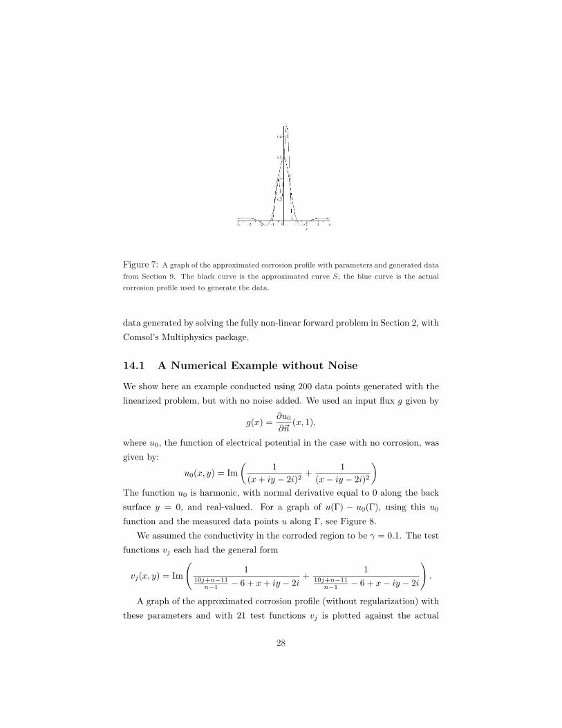
Figure 7: A graph of the approximated corrosion profile with parameters and generated data

from Section 9. The black curve is the approximated curve S; the blue curve is the actual

corrosion profile used to generate the data.

data generated by solving the fully non-linear forward problem in Section 2, with

Comsol’s Multiphysics package.

14.1 A Numerical Example without Noise

We show here an example conducted using 200 data points generated with the

linearized problem, but with no noise added. We used an input flux g given by

g(x) =∂u0

∂~n(x, 1),

where u0, the function of electrical potential in the case with no corrosion, was

given by:

u0(x, y) = Im(

1(x + iy − 2i)2

+1

(x− iy − 2i)2

)

The function u0 is harmonic, with normal derivative equal to 0 along the back

surface y = 0, and real-valued. For a graph of u(Γ) − u0(Γ), using this u0

function and the measured data points u along Γ, see Figure 8.

We assumed the conductivity in the corroded region to be γ = 0.1. The test

functions vj each had the general form

vj(x, y) = Im

(1

10j+n−11n−1 − 6 + x + iy − 2i

+1

10j+n−11n−1 − 6 + x− iy − 2i

).

A graph of the approximated corrosion profile (without regularization) with

these parameters and with 21 test functions vj is plotted against the actual

28

corrosion profile in Figure 9. In this case, the unregularized approximation was

sufficient, due to the lack of noise.

Figure 8: A graph of u(Γ)− u0(Γ), using the u0 and generated data points u from 14.1.

29

Figure 9: A graph of the approximated corrosion profile with parameters and generated

data from Section 14.1 (without regularization). The red curve is the approximated curve S;

the blue curve is the actual corrosion profile used to generate the data.

14.2 A Numerical Example with Nonlinear Data

We show here another example conducted using 200 data points generated by

Comsol’s Multiphysics program to solve the fully nonlinear problem. We used

input flux g given by

g(x) =∂u0

∂~n(x, 1),

where u0, the function of electrical potential in the case with no corrosion, was

given by:

u0(x, y) = Im(

1(x + iy − 2i)2

+1

(x− iy − 2i)2

).

As before, the function u0 is harmonic, with normal derivative equal to 0 along

the back surface (where y = 0), and real-valued. For a graph of u(Γ) − u0(Γ),

using this u0 function and the generated data points u along Γ, see Figure 10.

We again assumed the conductivity in the corroded region to be γ = 0.1.

The test functions vj each had the general form

vj(x, y) = Im

(1

10j+n−11n−1 − 6 + x + iy − 2i

+1

10j+n−11n−1 − 6 + x− iy − 2i

).

A graph of the approximated corrosion profile (before regularization) with

these parameters is plotted against the actual corrosion profile in Figure 11.

30

Notice again the extreme oscillations in the approximation before we employed

our method of regularization.

A graph of the approximated corrosion profile after regularization, with the

same parameters as in Figure 11 and with calculated threshold value t = 0.42,

is plotted against the actual corrosion profile in Figure 12.

Figure 10: A graph of u(Γ)− u0(Γ) with data generated from Comsol Multiphysics solving

the fully nonlinear problem.

Figure 11: A graph of the approximated corrosion profile using data generated by solving

the nonlinear problem (before regularization). The red curve is the approximated curve S;

the blue curve is the actual corrosion profile used to generate the data.

31

Figure 12: A graph of the approximated corrosion profile using the same data as in Figure

11, after regularization. The black curve is the approximated curve S; the blue curve is the

actual corrosion profile used to generate the data.

15 Conclusion and Future Work

Consider a two-dimensional region, Ω, with an accessible surface, Γ, and an inac-

cessible back surface that is partially corroded. We have shown that it is possible

to reconstruct the profile of this corrosion using measurements of electrical po-

tential on Γ. The methods for this reconstruction prove to be fairly accurate

considering the ill-posedness of the inverse problem. Ill-posedness was inves-

tigated through error analysis, and mitigated with a regularization procedure.

We have also shown that, although a unique solution cannot be presented with

only one reading of electrical potential on Γ, if two corrosion profiles generate

the same potential data along Γ they must have a non-zero point of intersection

on their supported domains.

We would like to investigate other aspects of this problem in the future.

First, we would like to test the precision of our algorithm. The numerical tests

we performed were all done with one section of corrosion on the back surface of

Ω. We would like to see how our algorithm handles the presence of two corrosion

profiles. How close together can the profiles be before the algorithm no longer

recognizes them as two separate entities?

We would also like to improve our algorithm for the approximation of the

function S(x). Although the algorithm we have created approximates the cor-

rosion profile closely, it does not do so exactly. Further precision in determining

32

the threshold values used in the singular value decomposition regularization

procedure may improve the algorithm. Considering the possibility of using a

different regularization method may also prove useful in this endeavor.

Extending this problem to electrothermal imaging is also something we want

to pursue. Does the generation of heat due to current flow in the corroded re-

gion allow the corrosion profile to be reconstructed more easily or accurately?

We would like to investigate whether or not solution uniqueness in the fully

non-linear case can be proven electrothermally despite the inability to do so

with purely electrical data.

Ultimately, we would like to extend all of these results to the three-dimensional

case where Ω is now a three-dimensional box or rod, and the corrosion profile

is a surface. This extension would allow our methods to be used in corrosion

detection in the field.

References

[1] Cakoni, F. and Kress, R. “Integral equations for inverse problems in cor-

rosion detection from partial Cauchy data.” Inverse Prob. Imaging 1 pp.

229-45. 2007.

[2] Strauss, Walter A. Partial Differential Equations: An Introduction. pp.

173-174. New York: John Wiley and Sons, Inc. 1992.

33